Dust–Gas Scaling Relations and OH Abundance in the Galactic ISM

Hiep Nguyen1,2 , J. R. Dawson1,2 , M.-A. Miville-Deschênes3,4, Ningyu Tang5 , Di Li5,6 , Carl Heiles7, Claire E. Murray8 ,Snežana Stanimirović9, Steven J. Gibson10, N. M. McClure-Griffiths11 , Thomas Troland12, L. Bronfman13 , and R. Finger141 Department of Physics and Astronomy and MQ Research Centre in Astronomy, Astrophysics and Astrophotonics, Macquarie University, NSW 2109, Australia

van-hiep.nguyen@hdr.mq.edu.au2 Australia Telescope National Facility, CSIRO Astronomy and Space Science, P.O. Box 76, Epping, NSW 1710, Australia3 Institut d’Astrophysique Spatiale, CNRS, Univ. Paris-Sud, Université Paris-Saclay, Bât. 121, F-91405, Orsay Cedex, France4 Laboratoire AIM, Paris-Saclay, CEA/IRFU/DAp—CNRS—Université Paris Diderot, F-91191, Gif-sur-Yvette Cedex, France

5 CAS Key Laboratory of FAST, NAOC, Chinese Academy of Sciences, People’s Republic of China6 University of Chinese Academy of Sciences, Beijing 100049, People’s Republic of China

7 Department of Astronomy, University of California, Berkeley, 601 Campbell Hall 3411, Berkeley, CA 94720-3411, USA8 Space Telescope Science Institute, 3700 San Martin Drive, Baltimore, MD 21218, USA

9 Department of Astronomy, University of Wisconsin-Madison, 475 North Charter Street, Madison, WI 53706, USA10 Department of Physics and Astronomy, Western Kentucky University, Bowling Green, KY 42101, USA

11 Research School of Astronomy and Astrophysics, Australian National University, Canberra, ACT 2611, Australia12 Department of Physics and Astronomy, University of Kentucky, Lexington, Kentucky 40506, USA

13 Departamento de Astronomía, Universidad de Chile, Casilla 36, Santiago de Chile, Chile14 Astronomy Department, Universidad de Chile, Camino El Observatorio 1515, 1058 Santiago, ChileReceived 2018 February 19; revised 2018 May 21; accepted 2018 May 24; published 2018 July 20

Abstract

Observations of interstellar dust are often used as a proxy for total gas column density NH. By comparing Planckthermal dust data (Release 1.2) and new dust reddening maps from Pan-STARRS 1 and 2MASS, with accurate(opacity-corrected) H I column densities and newly published OH data from the Arecibo Millennium survey and21-SPONGE, we confirm linear correlations between dust optical depth τ353, reddening E(B−V), and the totalproton column density NH in the range (1–30)× 1020 cm−2, along sightlines with no molecular gas detectionsin emission. We derive an NH/E(B−V ) ratio of (9.4± 1.6)×1021 cm−2 mag−1 for purely atomic sightlinesat b 5> ∣ ∣ , which is 60% higher than the canonical value of Bohlin et al. We report a ∼40% increase in opacityσ353=τ353/NH, when moving from the low column density (NH<5× 1020 cm−2) to the moderate columndensity (NH>5× 1020 cm−2) regime, and suggest that this rise is due to the evolution of dust grains in the atomicinterstellar medium. Failure to account for H I opacity can cause an additional apparent rise in σ353 of the order of afurther ∼20%. We estimate molecular hydrogen column densities NH2 from our derived linear relations, and hencederive the OH/H2abundance ratio of XOH∼1×10−7 for all molecular sightlines. Our results show no evidenceof systematic trends in OH abundance with NH2 in the range NH2∼(0.1−10)×1021 cm−2. This suggests thatOH may be used as a reliable proxy for H2in this range, which includes sightlines with both CO-dark andCO-bright gas.

Key words: dust, extinction – ISM: clouds – ISM: molecules

1. Introduction

Observations of neutral hydrogen in the interstellar medium(ISM) have historically been dominated by two radio spectrallines: the 21 cm line of atomic hydrogen (H I) and themicrowave emission from carbon monoxide (CO), particularlythe CO(J=1–0) line. The former provides direct measure-ments of the warm neutral medium (WNM), and the coldneutral medium (CNM), which is the precursor to molecularclouds. The latter is widely used as a proxy for molecularhydrogen (H2), often via the use of an empirical “X-factor,”(e.g., Bolatto et al. 2013). The processes by which CNM andmolecular clouds form from warm atomic gas sows the seeds ofstructure into clouds, laying the foundations for star formation.Being able to observationally track the ISM through thistransition is of key importance.

However, there is strong evidence for gas not seen in eitherH I or CO. This undetected material is often called “dark gas,”following Grenier et al. (2005). These authors found an excessof diffuse gamma-ray emission from the Local ISM, withrespect to the expected flux due to cosmic-ray interactions withthe gas mass estimated from H I and CO. Similar conclusionshave been reached using many different tracers, including

γ-rays (e.g., Abdo et al. 2010; Ackermann et al. 2012, 2011),infrared emission from dust (e.g., Blitz et al. 1990; Reachet al. 1994; Douglas & Taylor 2007; Planck Collaboration et al.2011, 2014a), dust extinction (e.g., Paradis et al. 2012; Leeet al. 2015), C II emission (Pineda et al. 2013; Langeret al. 2014; Tang et al. 2016), and OH 18 cm emission andabsorption (e.g., Wannier et al. 1993; Liszt & Lucas 1996;Barriault et al. 2010; Allen et al. 2012, 2015; Engelke &Allen 2018).While a minority of studies have suggested that cold,

optically thick H I could account for almost all the missing gasmass (Fukui et al. 2015), CO-dark H2 is generally expected tobe a major constituent, particularly in the envelopes ofmolecular clouds (e.g., Lee et al. 2015). In diffuse molecularregions, H2 is effectively self-shielded, but CO is typicallyphotodissociated (Tielens & Hollenbach 1985a, 1985b; vanDishoeck & Black 1988; Wolfire et al. 2010; Glover & MacLow 2011; Lee et al. 2015; Glover & Smith 2016), meaningthat CO lines are a poor tracer of H2 in such environments.Indeed Herschel observations of C II suggest that between20%–75% of the H2 in the Galactic plane may be CO-dark(Pineda et al. 2013).

The Astrophysical Journal, 862:49 (18pp), 2018 July 20 https://doi.org/10.3847/1538-4357/aac82b© 2018. The American Astronomical Society. All rights reserved.

1

For the atomic medium, the mass of warm H I can becomputed directly from measured line intensities under theoptically thin assumption. However, cold H I with spintemperature Ts100 K suffers from significant optical deptheffects, leading to an underestimation of the total columndensity. This difficulty is generally addressed by combining H Iabsorption and emission profiles observed toward (andimmediately adjacent to) bright, compact continuum back-ground sources. Such studies find that the optically thinassumption underestimates the true H I column by no more thana few tens of percent along most Milky Way sightlines (e.g.,Dickey et al. 1983, 2000, 2003; Heiles & Troland 2003a,2003b; Liszt 2014a; Lee et al. 2015); though, the fractionmissed in some localized regions may be much higher (Bihret al. 2015).

Since dust and gas are generally well mixed, absorptiondue to dust grains has been widely used as a proxy for totalgas column density. Early work (e.g., Savage & Jenkins1972, Bohlin et al. 1978) observed Lyα and H2absorptionin stellar spectra to calibrate the relationship betweentotal hydrogen column density NH, and the color excessE(B−V ). Similar work was carried out by comparing X-rayabsorption with optical extinction, AV (Reina & Tarenghi 1973,Gorenstein 1975). Bohlin et al’s value of NH/E(B−V )=5.8×1021 cm−2 mag−1 has become a widely accepted standard.

Dust emission is also a powerful tool and requires nobackground source population. The dust emission spectrum inthe bulk of the ISM peaks in the FIR-to-millimeter range, andarises mostly from large grains in thermal equilibrium with theambient local radiation field (Draine 2003, Draine & Li 2007).It has long been recognized that FIR dust emission couldpotentially be a better tracer of NH than H I and CO (de Vrieset al. 1987, Heiles et al. 1988, Blitz et al. 1990; Reachet al. 1994). An excess of dust intensity and/or optical depthabove a linear correlation with NH (as measured by H I and CO)is typically found in the range AV=0.3–2.7 mag (PlanckCollaboration et al. 2011, 2014a, 2014b; Martin et al. 2012),consistent with the range where CO-dark H2can exist.Alternative explanations cannot be definitively ruled out,however. These include (1) the evolution of dust grains acrossthe gas phases, (2) underestimation of the total gas column dueto significant cold H I opacity, and (3) insufficient sensitivityfor CO detection. It has also been impossible to rule outremaining systematic effects in the Planck data or bias in theestimate of τ353introduced by the choice of the modifiedblackbody model.

In this study, we examine the correlations betweenaccurately derived H I column densities and dust-based proxiesfor NH. We make use of opacity-corrected H I column densitiesderived from two surveys: the Arecibo Millennium Survey(MS, Heiles & Troland 2003b, hereafter HT03), and 21-SPONGE (Murray et al. 2015), both of which used on-/off-source measurements toward extragalactic radio continuumsources to derive accurate physical properties for the atomicISM. We also make use of archival OH data from theMillennium Survey, recently published for the first time in acompanion paper, Li et al. (2018). OH is an effective tracer ofdiffuse molecular regions (Wannier et al. 1993; Liszt &Lucas 1996; Barriault et al. 2010; Allen et al. 2012, 2015; Xuet al. 2016; Li et al. 2018), and has recently been surveyed at

high sensitivity in parts of the Galactic plane (Dawsonet al. 2014; Bihr et al. 2015). There exists both theoreticaland observational evidence for the close coexistence ofinterstellar OH and H2. Observationally, they appear to residein the same environments, as evidenced by tight relationsbetween their column densities (Weselak & Krełowski 2014).Theoretically, the synthesis of OH is driven by the ions O+ andH3

+ but requires H2as the precursor; once H2becomesavailable, OH can be formed efficiently through the charge-exchange chemical reactions initiated by cosmic-ray ionization(van Dishoeck & Black 1986). Here we combine H I, OH, anddust data sets to obtain new measurements of the abundanceratio, XOH=NOH/NH2—a key quantity for the interpretation ofOH data sets.The structure of this article is as follows. In Section 2, the

observations, the data processing techniques, and correctionson H I are briefly summarized. In Section 3, the results fromOH observations are discussed. Section 4 discusses therelationship between τ353, E(B−V ) and NH in the atomicISM. We finally estimate the OH/H2abundance ratio inSection 5 before concluding in Section 6.

2. Data Sets

In this study, we use the all-sky optical depth (τ353) map ofthe dust model data measured by Planck/IRAS (PlanckCollaboration et al. 2014a—hereafter PLC2014a), the red-dening E(B−V ) all-sky map from Green et al. (2018), H Idata from both the 21-SPONGE Survey (Murray et al. 2015)and the Millennium Survey (Heiles & Troland 2003a, HT03),OH data from the Millennium Survey (Li et al. 2018), and COdata from the Delingha 14 m Telescope, the Caltech Sub-millimeter Observatory (CSO), and the IRAM 30 m telescope(Li et al. 2018).

2.1. H I and OH

H I data from the Millennium Arecibo 21 cm Absorption-Line Survey (hereafter MS) was taken toward 79 strong radiosources (typically S2 Jy) using the Arecibo L-wide receiver.The two main lines of ground state OH at 1665.402 and1667.359MHz were observed simultaneously toward 72positions, and OH absorption was detected along 19 of thesesightlines (see also Li et al. 2018). The observations aredescribed in detail by HT03. Briefly, their so-called Z16observation pattern consists of one on-source absorptionspectrum toward the background radio source and 16 off-source emission spectra with the innermost positions at 1.0HPBW and the outermost positions at 2 HPBW from thecentral source. The off-source “expected” emission spectrum,the emission profile we would observe in the absence of thecontinuum source, is then estimated by modeling the 17-pointmeasurements. In this work, we use the published values ofHT03 for the total H I column density, NH I (scaled as describedbelow), and use the off-source (expected) MS emission profilesto compute the H I column density under the optically thinassumption, NH I

* , where required. We compute OH columndensities ourselves, as described in Section 3. All OH emissionand absorption spectra are scaled to a main-beam temperaturescale using a beam efficiency of ηb=0.5 (Heiles et al. 2001),

2

The Astrophysical Journal, 862:49 (18pp), 2018 July 20 Nguyen et al.

appropriate if the OH is not extended compared to the Arecibobeam size of 3′.

In order to increase the source sample, we also use H I datafrom the Very Large Array (VLA) 21-SPONGE Survey, whichobserved 30 continuum sources, including 16 in common withthe Millennium Survey sample (Murray et al. 2015). 21-SPONGE used on-source absorption data from the VLA,combining them with off-source emission profiles observedwith Arecibo. Murray et al. (2015) report an excellentagreement between the optical depths measured by the twosurveys, demonstrating that the single dish Arecibo absorptionprofiles are not significantly contaminated with resolved 21 cmemission. Note that in this work we have used an updatedscaling of the 21-SPONGE emission profiles, which applies abeam efficiency factor of 0.94 to the Arecibo spectra. The totalnumber of unique sightlines presented in this work is therefore93. The locations of all observed sources in Galacticcoordinates are presented in Figure 1. Where sources wereobserved in both the MS and 21-SPONGE, we use theMS data.

2.1.1. H I Intensity Scale Corrections

We check our NH I* against the Leiden–Argentine–Bonn

survey (LAB, Hartmann & Burton 1997; Kalberla et al. 2005)and the HI4PI survey (HI4PI Collaboration et al. 2016). Bothare widely regarded as a gold standard in the absolutecalibration of Galactic H I. We find that the optically thincolumn densities derived from 21-SPONGE are consistent withLAB and HI4PI. However, the MS values are systematicallylower than both LAB and HI4PI by a factor of ∼1.14. Apossible explanation for this difference lies in the fact that (in

contrast to 21-SPONGE) the MS did not apply a main-beamefficiency.To bring the MS data set in-line with LAB, HI4PI, and 21-

SPONGE, one might assume that both the on-source and off-source spectra must be rescaled, and the opacity-correctedcolumn densities recomputed according to the method of HT03(or equivalent). However, NH I may in fact be obtained from thetabulated values of HT03, with no need to perform a fullreanalysis of the data. For warm components, the tabulatedvalues of NH I are simply scaled by 1.14—appropriate sincethese were originally computed directly from the the integratedoff-source (expected) profiles under the optically thin assump-tion. For cold components, we recall that the radiative transferequations for the on-source and off-source (expected) spectra inthe MS data set are given by:

T v T T e T e T1 1BON

bg c s rxv v= + + - +t t- -( ) ( ) ( ) ( )

T v T e T e T1 , 2BOFF

bg s rxv v= + - +t t- -( ) ( ) ( )

where T vBOFF ( ) and T vB

ON ( ) are the main-beam temperatures ofthe off-source spectrum and on-source spectrum, respectively.Ts is the spin temperature, τv is the optical depth, Trx is thereceiver temperature (∼25 K), and Tc is the main-beamtemperature of the continuum source, obtained from the line-free portions of the on-source spectrum. Tbg is the continuumbackground brightness temperature including the 2.7 K iso-tropic radiation from CMB and the Galactic synchrotronbackground at the source position. Equations (1) and (2) maybe solved for τv and Ts:

eT v T v

T, 3B

ONBOFF

c

v =-t- ( ) ( ) ( )

Figure 1. Locations of all 93 sightlines considered in this study, overlaid on the map of dust optical depth τ353. Squares show H I absorption detections (93/93); redcircles show OH absorption detections (19/72); black circles show nondetections (51/72); red triangles show CO detections (19/44); and black triangles shownondetections (25/44). For purely atomic sightlines (those with no molecular detection at the threshold discussed in Section 4), the squares are colored red. Note thatthe absence of a symbol indicates that the sightline was not observed in that particular tracer. The labeled sightline toward 3C132 (far left) shows the single positiondetected in H I and OH but not detected in CO emissions. The “X” marker labels the center of the Milky Way. Note that the symbols for a small number of sightlinesentirely overlap due to their proximity on the sky.

3

The Astrophysical Journal, 862:49 (18pp), 2018 July 20 Nguyen et al.

TT v T e T

e1. 4s

BOFF

bg rxv

v=

- -

-

t

t

-

-

( )( )

From Equation (3), it is clear that optical depth is unchanged byany rescaling, which will affect both the numerator anddenominator of the expression identically. Only Ts must berecomputed. This is done on a component-by-component basisfrom the tabulated Gaussian fit parameters for peak opticaldepth, τ0, peak brightness temperature (scaled by 1.14), and thelinewidth Δv. The corrected NH I is obtained from

N T v

10 cm1.94

K km s, 5H

18 2 0s

1I t=

D- -[ ]

· ·[ ]

·[ ]

( )

where the factor 1.94 includes the usual constant 1.8224 andthe 1.065 arising from the integration over the Gaussian lineprofile.

2.1.2. NH I versus NH I*

We show in Figure 2 the correlation between NH I and NH I*

toward all 93 positions. While optically thin H I column densityis comparable with the true column density in diffuse/low-density regions with NH I5× 1020 cm−2, opacity effectsstart to become apparent above ∼5× 1020 cm−2.

If a linear fit is performed to the data, the ratio f=NH I/NH I*

may be described as a function of log(NH I* /1020) with a slope

of (0.19± 0.02) and an intercept of (0.89± 0.02) (see also Leeet al. 2015). Alternatively, a simple isothermal correction to theoptically thin NH I

* data with Ts∼144 K also yields a goodagreement with our data points, as illustrated in Figure 2 (seealso Liszt 2014b). This approach also better fits the low NH I

plateau, NH I<5× 1020 cm−2, below which NH I* ≈NH I.

While a single component with a constant spin temperature isa poor physical description of interstellar H I, it can provide areasonable (if crude) correction for opacity.

2.2. CO

As described in Li et al. (2018), a CO follow-up survey wasconducted toward 44 of the sightlines considered in this work.

The J=1–0 transitions of 12CO, 13CO, and C18Owereobserved with the Delingha 13.7 m telescope in China.12CO(J=2–1) data for 45 sources and J=3–2 data for 8sources with strong 12CO emission were taken with the 10.4 mCSO on Maunakea, with further supplementary data obtainedby the IRAM 30m telescope. In this work, we use CO datasolely to identify and exclude from some parts of the analysispositions with detected CO-bright molecular gas—comprising19 of the 44 observed positions. These positions are identifiedin Figure 1.

2.3. Dust

To trace the total gas column density NH, we use publiclyavailable all-sky maps of the 353 GHz dust optical depth (τ353)from the Planck satellite. The τ353map was obtained by amodified blackbody (MBB) fit to the first 15 months of 353,545, and 857 GHz data, together with IRAS 100 micron data(for details, see PLC2014a). The angular resolution of this dataset is 5 arcmin. In this work, we use the R1.20 data release inHealpix15 format (Górski et al. 2005). For dust reddening, weemploy the newly released all-sky 3D dust map of Green et al.(2018) at an angular resolution of 3 4–13 7, which was derivedfrom 2MASS and the latest Pan-STARRS 1 data photometry.In contrast to emission-based dust maps that depend on themodeling of the temperature, optical depth, and the shape ofthe emission spectrum, in maps based on stellar photometryreddening values are more directly measured and notcontaminated from zodiacal light or large-scale structure. Herewe convert the Green et al. (2018) Bayestar17 dust map toE(B−V ) by applying a scaling factor of 0.884, as described inthe documentation accompanying the data release.16

3. OH Data Analysis

The Millennium Survey OH data consists of on-source andoff-source “expected” spectra for each of the OH lines. In ourcompanion paper (Li et al. 2018), we use the method of HT03to derive OH optical depths, excitation temperatures andcolumn densities. Namely, we obtain solutions for theexcitation temperature, Tex, and τ via Gaussian fitting (to boththe on-source and off-source spectra) that explicitly includesthe appropriate treatment of the radiative transfer. In the presentwork, we use a simpler channel-by-channel method for thederivation of Tex.The radiative transfer equations for the on-source and off-

source (expected) spectra are identical to those for H I, givenabove in Equations (1) and (2). All terms and their meaningsare identical, with the exception that the spin temperature, Ts isreplaced by Tex. Tbg is the continuum background brightnesstemperature including the 2.7 K isotropic radiation from CMBand the Galactic synchrotron background at the source position.For consistency with HT03 and Li et al. (2018), we estimate thesynchrotron contribution at 1665.402 and 1667.359MHz fromthe 408MHz continuum map of Haslam et al. (1982), byadopting a temperature spectral index of 2.8, such that

T T2.7 408 , 6bg bg,408 OH2.8n= + -( ) ( )

resulting in typical values of around 3.5 K. The backgroundcontinuum contribution from Galactic H II regions may be

Figure 2. Ratio f=NH I/NH I* as a function of opacity-corrected NH I along 93sightlines from the MS and 21-SPONGE surveys. Circles show accurate NH I

obtained via on- and off-source observations (HT03; scaled as described in thetext), with the 34 atomic sightlines (selection criteria described in Section 4)filled gray and all other points filled black. Red triangles show NH I obtainedfrom NH I* assuming a single isothermal component of Ts∼144 K. The verticaldashed line is plotted at NH I=5 × 1020 cm−2; the horizontal dashed linemarks where NH I=NH I* .

15 http://healpix.sourceforge.net16 http://argonaut.skymaps.info/usage

4

The Astrophysical Journal, 862:49 (18pp), 2018 July 20 Nguyen et al.

safely ignored, since the continuum sources we observed areeither at high Galactic latitudes or Galactic anti-center long-itudes. Thus, in line-free portions of the off-source spectra:

T v T T . 7BOFF

bg rx= +( ) ( )

In the absence of information about the true gas distribution,we assume that OH clouds cover fully both the continuumsource and the main beam of the telescope. We may thereforesolve Equations (1) and (2) to derive Tex and τv for each of theOH lines, as shown in Equations (3) and (4) for the case of H I.

We fit each OH opacity spectrum (cf. Equation (3)) with aset of Gaussian profiles to obtain the peak optical depth (τ0,n),central velocity (v0,n), and FWHM (Δvn) of each component, n.Equation (4) is then used to calculate excitation temperaturespectra. Examples of e vt- , TB

OFF, and Tex spectra are shown inFigure 3, together with their associated Gaussian fits. It can beseen that the Tex spectra are approximately flat within theFWHM of each Gaussian component. We therefore compute anexcitation temperature for each component from the mean Texin the range v0,n±Δv/2.

Figure 4 compares the τ0 and Tex values obtained from ourmethod with those of Li et al. (2018), demonstrating that thetwo methods generally return consistent results. Minordifferences arise only for the most complex sightlines throughthe Galactic plane (G197.0+1.1, T0629+10), where the spectraare not simple to analyze; however, even these points aremostly consistent to within the errors.

We compute total OH column densities, NOH, independentlyfrom both the 1667 and 1665MHz lines via:

N T v

10 cm2.39

K km s, 8OH,1667

14 2 1667ex,1667 1667

2t=

D- -[ ]

· ·[ ]

·[ ]

( )

N T v

10 cm4.30

K km s, 9OH,1665

14 2 1665ex,1665 1665

2t=

D- -[ ]

· ·[ ]

·[ ]

( )

where the constants include Einstein A-coefficients ofA1667=7.778×10−11 s−1 and A1665=7.177×10−11 s−1

for the OH main lines (Destombes et al. 1977). All values ofτ0, Tex, and NOH are tabulated in Table 1.

4. Dust-based Proxies for Total NeutralGas Column Density

In this section, we will investigate the correlations betweendust properties and the total gas column density NH.Specifically, we consider dust optical depth at 353 GHz, τ353,and reddening, E(B−V ), with data sets sourced as describedin Section 2.3. When these quantities are used as proxies forNH, a single linear relationship between the measured quantityand NH is typically assumed. In this work, our H I data setprovides accurate (opacity-corrected) atomic column densities,while complementary OH and CO data allow us to identify andexclude sightlines with molecular gas (dark or not). We aretherefore able to measure τ353/NH and E(B−V )/NH along asample of purely atomic sightlines for which NH is very wellconstrained.In the following, we consider 34/93 sightlines to be “purely

atomic.” These are defined as either (a) sightlines where COand OH were observed and not detected in emission (16/93),or (b) sightlines where CO was not observed but OH wasobserved but not detected (18/93 sightlines). In both cases, werequire that OH be undetected in the 1667MHz line to adetection limit of NOH<1×1013 cm−2 (see Li et al. 2018),which excludes some positions with weaker continuum back-ground sources. We may confidently assume that thesesightlines contain very little or no H2 and note that all butone of them lie outside the Galactic plane ( b 10> ∣ ∣ ). Figure 5shows maps of the immediate vicinity of these sightlines in τ353and E(B−V ). Identical maps for the 19 sightlines with OHdetections (see also Section 5), are shown in Figure 6.In all of the following subsections, NH is taken to be equal to

NH I, the opacity-corrected H I column density, as derived alongsightlines with no molecular gas detected in emission.

Figure 3. Example of OH 1667 MHz e vt- (top), expected TBOFF (middle), and

Tex (bottom) spectra for the source P0428+20. The FWHM of the Gaussian fitsto the absorption profile are used to define the range over which Tex iscomputed for each component, shown as white regions in the bottom panel.

Figure 4. Comparison between derived values of the peak optical depth τ (leftpanel), and Tex (right panel) for both OH main lines, 1667 MHz (black) and1665 MHz (gray), as obtained from our companion paper by Li et al. (2018)and the present work. The dashed lines mark where the two values are equal.

5

The Astrophysical Journal, 862:49 (18pp), 2018 July 20 Nguyen et al.

Table 1Parameters for OH Main Lines

Source l/b OH(1665) OH(1667)

τ Vlsr ΔV Tex N(OH) τ Vlsr ΔV Tex N(OH)(Name) (°) (km s−1) (km s−1) (K) (1014 cm−2) (km s−1) (km s−1) (K) (1014 cm−2)

3C105 187.6/−33.6 0.0156±0.0003 8.14±0.01 0.95±0.03 4.65±1.86 0.29±0.12 0.0265±0.0004 8.17±0.01 0.94±0.02 3.95±0.95 0.23±0.063C105 187.6/−33.6 0.0062±0.0003 10.22±0.02 0.93±0.06 8.5±4.89 0.21±0.12 0.0104±0.0004 10.25±0.02 0.96±0.04 7.66±3.41 0.18±0.083C109 181.8/−27.8 0.0023±0.0003 9.15±0.11 1.03±0.26 18.28±27.06 0.18±0.27 0.0036±0.0004 9.24±0.05 0.75±0.12 24.58±8.7 0.16±0.063C109 181.8/−27.8 0.0036±0.0003 10.45±0.07 0.98±0.15 13.97±5.41 0.21±0.09 0.0053±0.0004 10.55±0.04 1.02±0.1 13.63±4.48 0.18±0.063C123 170.6/−11.7 0.0191±0.0007 3.65±0.06 1.19±0.11 10.92±3.26 1.05±0.33 0.0348±0.0009 3.71±0.04 1.22±0.07 10.92±2.69 1.1±0.283C123 170.6/−11.7 0.0431±0.0023 4.43±0.01 0.53±0.03 8.06±0.78 0.78±0.09 0.0919±0.0029 4.46±0.0 0.53±0.01 7.7±0.65 0.89±0.083C123 170.6/−11.7 0.0337±0.0008 5.37±0.01 0.91±0.03 11.59±4.3 1.53±0.57 0.0784±0.0009 5.47±0.01 0.92±0.01 8.79±2.57 1.5±0.443C131 171.4/−7.8 0.0065±0.0005 4.55±0.02 0.56±0.05 12.52±3.59 0.19±0.06 0.0117±0.0004 4.64±0.01 0.78±0.04 6.96±1.98 0.15±0.043C131 171.4/−7.8 0.0073±0.0006 6.81±0.06 2.91±0.23 8.94±4.54 0.82±0.42 0.0089±0.0005 5.84±0.03 0.67±0.08 11.04±2.07 0.16±0.043C131 171.4/−7.8 0.0166±0.0007 6.59±0.01 0.42±0.02 5.69±0.85 0.17±0.03 0.0319±0.0007 6.55±0.01 0.45±0.02 5.99±0.84 0.2±0.033C131 171.4/−7.8 0.0521±0.0007 7.23±0.0 0.55±0.01 5.91±0.64 0.72±0.08 0.0927±0.0005 7.22±0.0 0.65±0.01 5.98±0.34 0.85±0.053C132 178.9/−12.5 0.0033±0.0003 7.82±0.04 0.9±0.1 15.55±6.23 0.19±0.08 0.0056±0.0003 7.79±0.02 0.79±0.06 23.56±2.17 0.25±0.033C133 177.7/−9.9 0.1008±0.001 7.66±0.0 0.53±0.0 4.47±0.44 1.01±0.1 0.2132±0.0014 7.68±0.0 0.52±0.0 3.25±0.27 0.85±0.073C133 177.7/−9.9 0.0149±0.001 7.94±0.02 1.22±0.04 7.08±3.08 0.55±0.24 0.0333±0.0013 7.96±0.01 1.23±0.02 4.17±0.99 0.4±0.13C154 185.6/4.0 0.0266±0.0006 −2.32±0.02 0.74±0.03 2.69±1.93 0.23±0.16 0.0429±0.0006 −2.34±0.01 0.71±0.02 2.57±0.75 0.19±0.053C154 185.6/4.0 0.01±0.0006 −1.39±0.04 0.83±0.09 5.2±5.28 0.18±0.19 0.0181±0.0005 −1.34±0.02 0.94±0.05 4.46±1.79 0.18±0.073C154 185.6/4.0 0.0038±0.0005 2.23±0.07 1.14±0.17 5.83±6.56 0.11±0.12 0.0054±0.0004 2.19±0.05 1.57±0.13 0.54±8.69 0.01±0.173C167 207.3/1.2 0.0106±0.0019 18.46±0.12 1.49±0.35 4.75±17.95 0.32±1.22 0.009±0.0018 17.77±0.15 1.76±0.49 4.59±9.57 0.17±0.363C18 118.6/−52.7 0.0031±0.0003 −8.52±0.11 2.64±0.27 10.92±14.88 0.38±0.52 0.006±0.0003 −8.34±0.05 2.61±0.14 9.2±6.04 0.34±0.233C18 118.6/−52.7 0.0056±0.0004 −7.82±0.02 0.67±0.07 6.45±3.7 0.1±0.06 0.0079±0.0004 −7.85±0.01 0.6±0.04 4.83±1.6 0.05±0.023C207 213.0/30.1 0.015±0.0002 4.55±0.01 0.76±0.01 2.94±1.55 0.14±0.08 0.0266±0.0002 4.55±0.0 0.77±0.01 2.48±0.46 0.12±0.023C409 63.4/−6.1 0.0058±0.0011 14.59±0.27 1.68±0.35 11.31±8.53 0.47±0.38 0.0055±0.0015 14.68±0.33 1.52±0.4 7.83±11.73 0.16±0.243C409 63.4/−6.1 0.0204±0.0025 15.4±0.01 0.89±0.05 3.18±2.31 0.25±0.18 0.0275±0.0032 15.42±0.01 0.86±0.04 0.62±1.0 0.03±0.063C410 69.2/−3.8 0.0044±0.0006 6.32±0.04 1.89±0.15 13.41±11.22 0.47±0.4 0.0079±0.0005 6.38±0.02 2.32±0.09 6.4±5.25 0.28±0.233C410 69.2/−3.8 0.0089±0.0006 6.21±0.01 0.65±0.04 8.46±2.4 0.21±0.06 0.0193±0.0005 6.26±0.01 0.81±0.02 3.81±1.28 0.14±0.053C410 69.2/−3.8 0.0044±0.0003 10.7±0.03 0.71±0.07 10.06±5.89 0.13±0.08 0.0085±0.0002 10.71±0.02 0.81±0.04 4.15±3.09 0.07±0.053C410 69.2/−3.8 0.0054±0.0002 11.67±0.03 0.84±0.07 4.83±4.66 0.09±0.09 0.0115±0.0002 11.68±0.02 0.82±0.03 2.93±3.0 0.07±0.073C454.3 86.1/−38.2 0.0023±0.0001 −9.67±0.03 1.6±0.09 4.63±12.36 0.07±0.19 0.0044±0.0001 −9.54±0.01 1.25±0.04 8.13±6.06 0.1±0.083C75 170.3/−44.9 0.0071±0.0005 −10.36±0.04 1.3±0.12 3.45±5.41 0.14±0.21 0.014±0.0008 −10.36±0.03 1.22±0.09 3.51±1.56 0.14±0.064C13.67 43.5/9.2 0.0464±0.0043 4.85±0.05 1.1±0.12 10.43±2.77 2.28±0.69 0.0567±0.0057 4.89±0.05 1.12±0.14 10.34±2.13 1.55±0.44C22.12 188.1/0.0 0.0058±0.001 −2.84±0.07 0.79±0.19 6.54±7.03 0.13±0.14 0.0102±0.0011 −2.73±0.04 0.78±0.12 6.72±2.32 0.13±0.054C22.12 188.1/0.0 0.0172±0.0012 −1.78±0.02 0.56±0.05 5.07±2.12 0.21±0.09 0.0354±0.0013 −1.78±0.01 0.54±0.03 3.78±0.74 0.17±0.03G196.6+0.2 196.6/0.2 0.0044±0.0005 3.26±0.11 1.94±0.27 10.82±12.22 0.4±0.46 0.0062±0.0005 3.4±0.09 2.38±0.22 8.85±8.6 0.31±0.3G197.0+1.1 197.0/1.1 0.0126±0.0005 4.83±0.04 1.88±0.09 6.94±3.82 0.7±0.39 0.0191±0.001 4.73±0.04 1.65±0.1 4.8±2.17 0.36±0.16G197.0+1.1 197.0/1.1 0.0059±0.0009 7.46±0.05 0.65±0.11 0.31±10.58 0.0±0.17 0.0078±0.0015 7.34±0.06 0.65±0.14 1.61±5.87 0.02±0.07G197.0+1.1 197.0/1.1 0.0049±0.0005 17.01±0.12 2.47±0.28 10.99±9.9 0.57±0.52 0.0081±0.0034 16.26±0.17 0.91±0.3 6.45±2.95 0.11±0.08G197.0+1.1 197.0/1.1 0.0052±0.0015 17.59±0.03 0.25±0.08 9.87±1.81 0.05±0.03 0.0127±0.0013 17.38±0.2 1.46±0.35 5.46±4.35 0.24±0.2G197.0+1.1 197.0/1.1 0.0237±0.001 32.01±0.01 0.57±0.03 4.75±1.92 0.27±0.11 0.043±0.0017 32.01±0.01 0.54±0.02 3.96±1.04 0.22±0.06P0428+20 176.8/−18.6 0.0014±0.0002 3.6±0.08 1.01±0.19 13.48±7.8 0.08±0.05 0.0029±0.0003 3.54±0.03 0.69±0.08 4.45±9.98 0.02±0.05P0428+20 176.8/−18.6 0.0075±0.0002 10.7±0.02 1.09±0.04 13.49±3.45 0.47±0.12 0.0136±0.0002 10.7±0.01 1.1±0.02 12.72±1.62 0.45±0.06T0526+24 181.4/−5.2 0.0172±0.0073 7.55±0.29 1.9±1.13 13.7±15.65 1.91±2.59 0.043±0.0102 7.56±0.14 2.43±0.75 10.19±7.5 2.52±2.1T0629+10 201.5/0.5 0.0043±0.0022 0.16±0.0 0.65±0.4 4.16±2.97 0.05±0.05 0.0103±0.0035 0.35±0.0 1.18±0.41 3.25±1.93 0.09±0.07T0629+10 201.5/0.5 0.0387±0.0074 3.14±0.13 1.1±0.0 3.85±0.47 0.7±0.16 0.0577±0.0113 3.07±0.14 1.1±0.0 4.54±0.55 0.68±0.16T0629+10 201.5/0.5 0.0169±0.0015 1.46±0.07 1.39±0.26 2.19±2.11 0.22±0.22 0.0281±0.0029 1.51±0.08 1.23±0.25 2.9±0.91 0.24±0.09

6

TheAstro

physica

lJourn

al,

862:49(18pp),

2018July

20Nguyen

etal.

Table 1(Continued)

Source l/b OH(1665) OH(1667)

τ Vlsr ΔV Tex N(OH) τ Vlsr ΔV Tex N(OH)(Name) (°) (km s−1) (km s−1) (K) (1014 cm−2) (km s−1) (km s−1) (K) (1014 cm−2)

T0629+10 201.5/0.5 0.1607±0.0104 3.6±0.01 0.61±0.02 3.83±0.35 1.59±0.19 0.2536±0.0154 3.6±0.01 0.65±0.03 4.72±0.64 1.84±0.29T0629+10 201.5/0.5 0.0811±0.002 4.62±0.01 0.76±0.03 6.43±0.97 1.68±0.27 0.1553±0.0037 4.61±0.01 0.67±0.03 6.62±1.01 1.63±0.26T0629+10 201.5/0.5 0.0747±0.0018 6.09±0.02 1.06±0.05 5.44±1.58 1.84±0.54 0.1165±0.003 6.06±0.02 1.17±0.07 6.52±1.67 2.1±0.55T0629+10 201.5/0.5 0.0367±0.0031 7.0±0.02 0.49±0.06 4.36±0.68 0.33±0.07 0.0631±0.0056 7.0±0.02 0.5±0.06 4.2±0.3 0.31±0.05T0629+10 201.5/0.5 0.0174±0.0018 7.9±0.05 0.83±0.13 3.44±1.67 0.21±0.11 0.0307±0.003 7.91±0.05 0.82±0.13 3.65±1.21 0.22±0.08

7

TheAstro

physica

lJourn

al,

862:49(18pp),

2018July

20Nguyen

etal.

4.1. NH from Dust Optical Depth τ353

We adopt the all-sky map of dust optical depth τ353computed by PLC2014a. This was derived from an MBBempirical fit to IRAS and Planck maps at 3000, 857, 545, and353 GHz, described by the expression:

I B T353

. 10353 dustdust

tn

=n n

b⎜ ⎟⎛⎝

⎞⎠( ) ( )

Here, τ353, dust temperature, Tdust, and spectral index, βdust, arethe three free parameters, and Bν(Tdust) is the Planck functionfor dust at temperature Tdust which is, in this model, consideredto be uniform along each sightline (see PLC2014a for moredetails). The relation between dust optical depth and total gascolumn density can then be written as:

I

B Tr m N N , 11353

353

353 dust353 H H 353 Ht k m s= = =

( )( )

where σ353is the dust opacity, κ353 is the dust emissivity cross-section per unit mass (cm2 g−1), r is the dust-to-gas mass ratio,

μ is the mean molecular weight, and mH is the mass of ahydrogen atom.Figure 7 shows the correlation between NH and τ353. A tight

linear trend can be seen with a Pearson coefficient of 0.95. Thevalue of σ353from the orthogonal distance regression (Boggs& Rogers 1990) linear fit is (7.9± 0.6)× 10−27 cm2 H−1 (theintercept is set to 0), where the quoted uncertainties are the95% confidence limits estimated from pair bootstrap resam-pling. This is consistent to within the uncertainties with thatobtained by PLC2014a based on all-sky H I data from LAB,(6.6± 1.7)× 10−27 cm2 H−1. Note that here we have quotedthe PLC2014a measurement made toward low NH I positions,because the lack of any H I opacity correction in that workmakes this value the most reliable. However, our fit isconsistent with all of the σ353values presented in that work(which was based on the Planck R1.20 data release), to withinthe quoted uncertainties.Small systematic deviations from the linear fit, evident at the

high and low column density ends of the plot, are discussedfurther in Section 4.3.

Table 234 Atomic Sightlines

Sources l/b NH I NH I* στ(OH1667) NH2(upper limit)a τ353 E(B−V )(Name) (°) (1020 cm−2) (1020 cm−2) (10−4) (1020 cm−2) (10−6) (10−2 mag)

3C33 129.4/−49.3 3.25±0.0 3.2±0.1 12.14 0.6 2.16±0.07 3.54±0.423C142.1 197.6/−14.5 25.11±2.6 19.6±0.8 10.55 0.52 21.53±0.72 21.71±0.813C138 187.4/−11.3 22.9±1.1 19.9±0.3 5.02 0.25 21.63±0.81 17.47±0.593C79 164.1/−34.5 10.86±1.2 9.8±0.8 37.03 1.84 9.23±0.37 12.67±0.783C78 174.9/−44.5 11.69±0.5 10.3±0.2 13.25 0.66 12.45±0.63 14.64±1.073C310 38.5/60.2 4.29±0.1 4.0±0.1 16.19 0.8 3.48±0.15 2.75±0.533C315 39.4/58.3 5.48±0.4 4.7±0.0 12.96 0.64 3.98±0.09 5.63±0.263C234 200.2/52.7 1.84±0.0 1.9±1.1 12.66 0.63 0.78±0.03 1.64±0.563C236 190.1/54.0 1.38±0.0 1.3±1.2 10.72 0.53 0.7±0.03 2.04±0.493C64 157.8/−48.2 7.29±0.2 6.9±0.8 33.12 1.65 6.55±0.35 9.01±0.36P0531+19 186.8/−7.1 27.33±0.7 25.4±0.3 6.37 0.32 20.75±0.62 20.54±1.3P0820+22 201.4/29.7 4.82±0.2 4.8±1.1 7.09 0.35 3.73±0.11 2.56±0.43C192 197.9/26.4 4.56±0.1 4.5±0.1 20.66 1.03 3.38±0.08 4.05±0.533C98 179.8/−31.0 12.7±0.5 11.3±1.3 12.26 0.61 13.72±0.41 17.73±1.023C273 289.9/64.4 2.35±0.0 2.3±0.1 21.0 1.04 1.3±0.09 1.98±0.41DW0742+10 209.8/16.6 2.77±0.0 2.8±0.9 8.01 0.4 1.6±0.03 1.99±0.253C172.0 191.2/13.4 8.89±0.2 8.6±1.1 13.02 0.65 5.66±0.08 4.7±0.523C293 54.6/76.1 1.46±0.1 1.5±1.1 6.24 0.31 1.31±0.09 2.83±0.753C120 190.4/−27.4 18.17±2.1 10.7±0.1 28.29 1.41 29.26±1.08 22.74±1.03CTA21 166.6/−33.6 10.97±0.4 10.0±0.8 27.35 1.36 10.39±0.44 13.3±0.96P1117+14 240.4/65.8 1.79±0.0 1.8±0.3 15.0 0.75 1.5±0.04 2.73±0.543C264.0 237.0/73.6 1.97±0.0 2.0±0.4 6.29 0.31 1.64±0.08 2.88±0.343C208.1 213.6/33.6 3.15±0.1 3.2±0.2 18.67 0.93 3.12±0.04 2.93±0.433C208.0 213.7/33.2 3.41±0.1 3.5±0.2 19.69 0.98 3.38±0.07 4.37±0.474C32.44 67.2/81.0 1.23±0.0 1.3±0.6 9.88 0.49 0.81±0.02 1.94±0.293C272.1 280.6/74.7 2.82±0.0 2.8±0.3 10.24 0.51 1.73±0.28 2.43±0.314C07.32 322.2/68.8 2.43±0.0 2.4±0.3 30.7 1.53 2.32±0.06 4.3±0.413C245 233.1/56.3 2.39±0.0 2.4±0.2 11.36 0.56 2.22±0.06 2.71±0.363C348 23.0/29.2 6.56±0.2 6.0±0.1 16.51 0.82 5.7±0.15 9.8±0.333C286 56.5/80.7 2.33±0.1 2.4±2.7 7.13 0.35 0.81±0.05 2.75±0.744C13.65 39.3/17.7 10.56±0.2 9.9±0.1 20.01 0.99 11.8±0.39 15.63±0.63C190.0 207.6/21.8 3.21±0.0 3.4±0.9 17.57 0.87 2.41±0.03 1.96±0.423C274.1 269.9/83.2 2.74±0.0 2.6±0.1 13.13 0.65 2.34±0.02 2.64±0.423C298 352.2/60.7 2.39±0.4 2.6±0.1 10.69 0.53 1.3±0.07 1.97±0.39

Note.a Estimated from OH(1667) 3σ detection limits using Tex=3.5 K, FWHM=1 km s−1 and NOH/NH2=10−7 (see Section 5).

8

The Astrophysical Journal, 862:49 (18pp), 2018 July 20 Nguyen et al.

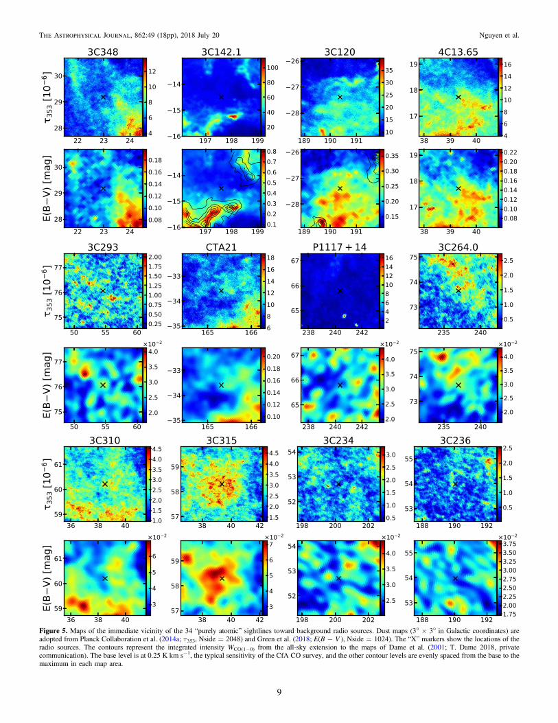
Figure 5. Maps of the immediate vicinity of the 34 “purely atomic” sightlines toward background radio sources. Dust maps (3°×3°in Galactic coordinates) areadopted from Planck Collaboration et al. (2014a; τ353, Nside=2048) and Green et al. (2018; E(B−V ), Nside=1024). The “X” markers show the locations of theradio sources. The contours represent the integrated intensity WCO(1−0) from the all-sky extension to the maps of Dame et al. (2001; T. Dame 2018, privatecommunication). The base level is at 0.25 K km s−1, the typical sensitivity of the CfA CO survey, and the other contour levels are evenly spaced from the base to themaximum in each map area.

9

The Astrophysical Journal, 862:49 (18pp), 2018 July 20 Nguyen et al.

In order to examine the possible contribution of moleculargas to NH along the 34 atomic sightlines, we estimate upperlimits on NH2 from the 3σ OH detection limits using an

abundance ratio of XOH=10−7 (see Section 5). Thesevalues are tabulated in Table 2, and the resulting upperlimits on NH are shown as gray triangles in Figure 7. As

Figure 5. (Continued.)

10

The Astrophysical Journal, 862:49 (18pp), 2018 July 20 Nguyen et al.

Figure 5. (Continued.)

11

The Astrophysical Journal, 862:49 (18pp), 2018 July 20 Nguyen et al.

Figure 6.Maps of the immediate vicinity of the 19 OH-detected sightlines toward background radio sources. Dust maps (3°×3°in Galactic coordinates) are adoptedfrom Planck Collaboration et al. (2014a; τ353, Nside = 2048) and Green et al. (2018; E(B − V), Nside = 1024). The “X” markers show the locations of the radiosources. The contours represent the integrated intensity WCO(1−0) from the all-sky extension to the maps of Dame et al. (2001; T. Dame 2018, private communication).The base level is at 0.25 K km s−1, the typical sensitivity of the CfA CO survey, and the other contour levels are evenly spaced from the base to the maximum in eachmap area.

12

The Astrophysical Journal, 862:49 (18pp), 2018 July 20 Nguyen et al.

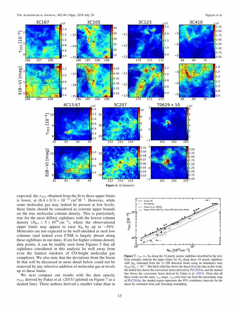
expected, the σ353obtained from the fit to these upper limitsis lower, at (6.4± 0.3)× 10−27 cm2 H−1. However, whilesome molecular gas may indeed be present at low levels,these limits should be considered as extreme upper boundson the true molecular column density. This is particularlytrue for the most diffuse sightlines with the lowest columndensity (NH I<5× 1020 cm−2), where the observationalupper limits may appear to raise NH by up to ∼50%.Molecules are not expected to be well-shielded at such lowcolumns (and indeed even CNM is largely absent alongthese sightlines in our data). Even for higher column densitydata points, it can be readily seen from Figures 5 that allsightlines considered in this analysis lie well away fromeven the faintest outskirts of CO-bright molecular gascomplexes. We also note that the deviations from the linearfit that will be discussed in more detail below could not beremoved by any selective addition of molecular gas at levelsup to these limits.

We next compare our results with the dust opacityσ353derived by Fukui et al. (2015) (plotted on Figure 7 as adashed line). These authors derived a smaller value than in

Figure 6. (Continued.)

Figure 7. τ353vs. NH along the 34 purely atomic sightlines described in the text.Gray triangles indicate the upper limits for NH along these 34 atomic sightlineswith NH2 estimated from the 3σ OH detection limits using an abundance ratioNOH/NH2=10−7. The thick solid line shows the linear fit to the data in this work,the dotted line shows the conversion factor derived by PLC2014a, and the dashedline shows the conversion factor derived by Fukui et al. (2015). (Note that allthese works use the same τ353 map). τ353 error bars are from the uncertainty mapof PLC2014a; the shaded region represents the 95% confidence intervals for thelinear fit, estimated from pair bootstrap resampling.

13

The Astrophysical Journal, 862:49 (18pp), 2018 July 20 Nguyen et al.

the present work (by a factor of ∼1.5), by restricting their fitto only the warmest dust temperatures, under the assumptionthat these most reliably select for genuinely optically thinH I. They then applied this factor to the Planck τ353 map(excluding b 15< ∣ ∣ and CO-bright sightlines) to estimateNH I, assuming that the contribution from CO-dark H2 wasnegligible. This resulted in NH I values ∼2–2.5 times higherthan under the optically thin assumption, and motivatedtheir hypothesis that significantly more optically thick H Iexists than is usually assumed. However, we find that whilethe σ353of Fukui et al. (2015) may be a good fit to somesightlines in the very low NH I regime (3× 1020 cm−2), itoverestimates NH I at larger column densities by ∼50%.Indeed, as will be discussed below, σ353 is not expected toremain constant as dust evolves. This (combined with some

contribution from CO-dark H2) may reconcile the apparentdiscrepancy between their findings and absorption/emission-based measurements of the opacity-corrected H I column.

4.2. NH from Dust Reddening E(B−V)

Reddening caused by the absorption and scattering of lightby dust grains is defined as:

E B VA

R Rr m N1.086 , 12V

V

V

VH H

km- = =( ) ( )

where AV is the dust extinction, RV is an empirical coefficientcorrelated with the average grain size, and all other symbols aredefined as before. In the Milky Way, RV is typically assumed tobe 3.1 (Schultz & Wiemer 1975), but it may vary between 2.5and 6.0 along different sightlines (Goodman et al. 1995;Draine 2003).

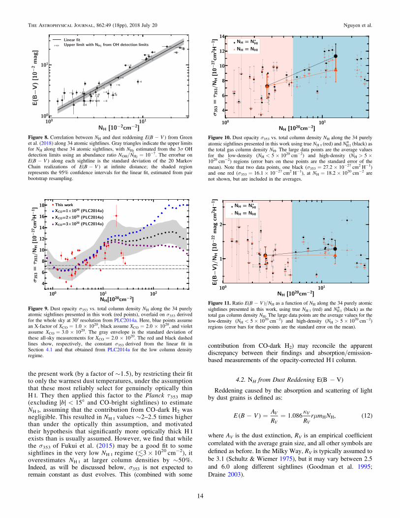
Figure 9. Dust opacity σ353 vs. total column density NH along the 34 purelyatomic sightlines presented in this work (red points), overlaid on σ353 derivedfor the whole sky at 30′ resolution from PLC2014a. Here, blue points assumean X-factor of XCO=1.0×1020, black assume XCO=2.0×1020, and violetassume XCO=3.0×1020. The gray envelope is the standard deviation ofthese all-sky measurements for XCO=2.0×1020. The red and black dashedlines show, respectively, the constant σ353derived from the linear fit inSection 4.1 and that obtained from PLC2014a for the low column densityregime.

Figure 10. Dust opacity σ353 vs. total column density NH along the 34 purelyatomic sightlines presented in this work using true NH I (red) and NH I* (black) asthe total gas column density NH. The large data points are the average valuesfor the low-density (NH<5 × 1020 cm−2) and high-density (NH>5 ×1020 cm−2) regions (error bars on these points are the standard error of themean). Note that two data points, one black (σ353=27.2 × 10−27 cm2 H−1)and one red (σ353=16.1 × 10−27 cm2 H−1), at NH=18.2 × 1020 cm−2 arenot shown, but are included in the averages.

Figure 11. Ratio E(B−V )/NH as a function of NH along the 34 purely atomicsightlines presented in this work, using true NH I (red) and NH I* (black) as thetotal gas column density NH. The large data points are the average values for thelow-density (NH<5 × 1020 cm−2) and high-density (NH>5 × 1020 cm−2)regions (error bars for these points are the standard error on the mean).

Figure 8. Correlation between NH and dust reddening E(B−V ) from Greenet al. (2018) along 34 atomic sightlines. Gray triangles indicate the upper limitsfor NH along these 34 atomic sightlines, with NH2 estimated from the 3σ OHdetection limits using an abundance ratio NOH/NH2=10−7. The errorbar onE(B−V ) along each sightline is the standard deviation of the 20 MarkovChain realizations of E(B−V ) at infinite distance; the shaded regionrepresents the 95% confidence intervals for the linear fit, estimated from pairbootstrap resampling.

14

The Astrophysical Journal, 862:49 (18pp), 2018 July 20 Nguyen et al.

The ratio N E B V 5.8 10 cm magH21 2 1á - ñ = ´ - -( ) (Bohlin

et al. 1978) is a widely accepted standard, used in many fields ofastrophysics to connect reddening measurements to gas columndensity. This value was derived from Lyα and H2lineabsorption measurements toward 100 stars (see also Savageet al. 1977), and has been replicated over the years via similarmethodology (e.g., Shull & van Steenberg 1985; Diplas &Savage 1994; Rachford et al. 2009). However, a number ofrecent works using H I 21 cm data have found significantlyhigher values (PLC2014a; Liszt 2014a; Lenz et al. 2017).

Here we use the all-sky map of E(B−V ) from Greenet al. (2018) to estimate the ratio NH/E(B−V ) for oursample of purely atomic sightlines, at b 5> ∣ ∣ . The resultsare shown in Figure 8. It can be seen that E(B−V ) and NH

are strongly linearly correlated, with a Pearson coefficientof 0.93. The ratio obtained from the linear fit isNH/E(B−V )=(9.4± 1.6)×1021 cm−2 mag−1 (the inter-cept is also set to be 0), where the quoted uncertainties arethe 95% confidence limits estimated from pair bootstrapresampling. This value is a factor of 1.6 higher than that inBohlin et al. (1978).

The value obtained here is consistent with the estimate ofLenz et al. (2017): NH/E(B−V )=8.8×1021 cm−2 mag−1 (nouncertainty is given in that work). These authors comparedoptically thin H I column density from HI4PI (Collaboration et al.2016) with various estimates of E(B−V ) from Schlegel et al.(1998), Peek & Graves (2010), Schlafly et al. (2014), PLC2014a,and Meisner & Finkbeiner (2015). We note that the estimate ofLenz et al. (2017) is only valid for NH<4× 1020 cm−2, where itseems safe to assume that the 21 cm emission is optically thin.Our value is also close to that of Liszt (2014a), who findNH I/E(B−V )=8.3×1021 cm−2 mag−1 (also given withoutuncertainty) for b 20 ∣ ∣ and 0.015E(B−V )0.075, bycomparing H I data from LAB and E(B−V ) from Schlegel et al.(1998). The methodology used by these two studies differs in anumber of details. For instance, Liszt (2014a) did not apply a gaincorrection to the Schlegel et al. (1998) map (whereas Lenzet al. 2017 scaled it down by 12%), and did not smooth it to theLAB angular resolution (30′). However, Liszt (2014a) did applyan empirical correction factor to account for H I opacity (albeitone whose effects on high-latitude sightlines was small). These

details may account for the difference between the values obtainedby these two otherwise similar studies.We also note that, like the present work, these studies did not

take into account the potential contribution of dust associatedwith the diffuse warm ionized gas (WIM). This would tend toproduce a flattening of the E(B−V ) versus NH I relation at lowNH I and therefore increase the value of NH I/E(B−V )artificially. Because we are able to accurately probe a largecolumn density range (up to 3×1021 cm−2), we would naivelyexpect our estimate of NH/E(B−V ) to be less affected byWIM bias than either Liszt (2014a) or Lenz et al. (2017; whichwould tend to have a greater effect on lower column datapoints). While more work is needed to quantify the contributionof the WIM on dust emission/absorption measurements at lowE(B−V ), we consider it unlikely to account for the differencebetween our work and historically lower measurements of theNH/E(B−V ) ratio.Despite minor differences between these three studies, it is

clear that they point to a NH I/E(B−V ) value of(∼8–9)×1021 cm−2 mag−1. This is 40%–60% higher thanthe traditional value of Bohlin et al. (1978), which has beenused by most models of interstellar dust as a reference point toset the dust-to-gas ratio (e.g., Draine & Fraisse 2009; Joneset al. 2013). We note that if NH is replaced with upper limits (asdiscussed in Section 4.1), NH/E(B−V ) climbs yet higher,leaving this key conclusion unaffected.

4.3. Disentangling the Effects of Grain Evolution and DarkGas on σ353

A number of studies have used the correlation between τ353and NH, particularly with regards to the search for dark gas(e.g., Planck Collaboration et al. 2011; Fukui et al. 2014, 2015;Reach et al. 2015). It is clear that τ353 and NH are in generallinearly correlated only if σ353 is a constant. However, it isrecognized that σ353 is sensitive to grain evolution, andsignificant variations in the ratio NH/τ353 have been observed,particularly when transitioning to the high-density, molecularregime (e.g., Planck Collaboration et al. 2014a, 2015; Okamotoet al. 2017; Remy et al. 2017). The origin of observedvariations in σ353 may relate to a change in dust properties viaκ353, and/or a variation in the dust-to-gas ratio r, but may alsoinclude a contribution due to the presence of dark gas, if this isunaccounted for in the estimated NH.PLC2014a presented the variation in σ353 with NH at 30′

resolution over the entire sky. In that work, NH was derivedfrom (NH I

* +XCOWCO), thus dark gas (both optically thick H Iand CO-dark H2) was unaccounted for. We reproduce their datain Figure 9. It can be seen that σ353 is roughly flat and at aminimum in a narrow, low column density range NH=(1−3)× 1020 cm−2, then increases linearly until NH=15×1020 cm−2, by which point it is almost a factor of 2 higher. Itthen remains approximately constant for the canonical value ofXCO=2.0×1020 cm−2 K−1 km−1 s. A key issue for dark gasstudies is disentangling how much of the initial rise in σ353 isdue to changing grain properties and how much is due to thecontribution of unseen material, whether it be opaque H I ordiffuse H2. (Note also the upturn in σ353 seen at the lowest NH,which may be due to the presence of unaccounted-for protonsin the warm ionized medium.)The column density range probed by our purely atomic

sightlines, NH=(1∼30)× 1020 cm−2 well samples the rangewhere σ353 undergoes its first linear increase. Dark gas is also

Figure 12. Left: NOH as a function of NH2obtained from the two NH proxies, E(B−V ) (blue) and τ353 (red). Right: XOH derived from the two proxies as afunction of NH2.

15

The Astrophysical Journal, 862:49 (18pp), 2018 July 20 Nguyen et al.

fully accounted for in our data, since H I is opacity-corrected,and no molecular gas is detected in emission along thesesightlines. To quantify the effect of ignoring H I opacity onσ353, we compare σ353deduced from the true, opacity-corrected NH I with that deduced under the optically thinassumption. The results are shown in Figure 10. In low columndensity regions (NH<5× 1020 cm−2), each σ353pair fromNH I and NH I

* are comparable. However, at higher columndensities (NH>5× 1020 cm−2) σ353from true NH I is system-atically lower than that measured from NH I

* . On average,σ353obtained from optically thin H I column density increasesby ∼1.6 when going from low to high column density regions;whereas σ353from true NH I increases by ∼1.4. This suggeststhat if H I opacity is not explicitly corrected for, it can accountfor around one-third (1/3) of the increase of σ353observedduring the transition from diffuse to dense atomic regimes. Theremaining of two-thirds (2/3) must arise due to changes in dustproperties.

From Equation (11), we see that σ353 is a function of thedust-to-gas mass ratio, r, and the dust emissivity cross-section,κ353, which depends on the composition and structure of dustgrains. Given the uncertainties on the efficiency of the physicalprocesses involved in the evolution of interstellar dust grains, itis difficult at this point to conclude if the variations of σ353observed here are due to an increase of the dust mass (i.e., r) orto a change in the dust emission properties (i.e., κ353). Usingthe dust model of Jones et al. (2013), Ysard et al. (2015)suggest that most of the variations in the dust emissionobserved by Planck in the diffuse ISM could be explained byrelatively small variations in the dust properties. Thatinterpretation would favor a scenario in which the increase ofσ353 from diffuse to denser gas is caused by the growth of thinmantles via the accretion of atoms and molecules from the gasphase. Even though this process would increase the mass ofgrains (and therefore increase r), the change of the structure ofthe grain surface would lead to a larger increase in κ353.Alternatively, it is possible that this systematic variation ofτ353/NH could be due to residual large-scale systematic effectsin the Planck data, or to the fact that the modified blackbodymodel introduces a bias in the estimate of τ353. Neither of theseexplanations can be ruled out.

Figure 9 shows σ353as a function of NH superimposed onthe results from PLC2014a. It can be seen that we observe asimilar rise in σ353 in the column density range(∼5–30)×1020 cm−2, but less extreme. In particular, mostof our data points in the higher column density range(NH>5× 1020 cm−2) are found below the PLC2014a trend,which is derived from the mean values of σ353over the wholesky in NH bins. This is true even if we use NH I

* rather than NH I

to derive σ353, indicating that optically thick H I alone cannotshift our data points high enough for a perfect match. This isconsistent with the fact that we are examining purely atomicsightlines, and likely happens because we are samplingcomparatively low number densities (nH10–100 cm−3; amixture of WNM and CNM), whereas the sample in PLC2014aincludes molecular gas in the NH bins, presumably with ahigher κ353. However, in diffuse regions with NH<5×1020 cm−2, the mean value of σ353 from our sample iscomparable with that from PLC2014a.

4.4. E(B−V) as the More Reliable Proxy for NH?

We have seen that along 34 atomic sightlines E(B−V )shows a tight linear correlation with NH in the column densityrange NH=(1∼30)× 1020 cm−2. τ353also shows a goodlinear relation with NH but with systematic deviations asdescribed above.Figure 11 replicates Figure 10 but for E(B−V ) rather than

τ353. Although the sample used here is small, these figuresdemonstrate clearly that the ratio E(B−V )/NH is more stablethan τ353/NH over the range of column densities and sightlinescovered by our analysis. In fact, with NH corrected for opticaldepth effects, our data are compatible with a constant value forE(B−V )/NH, up to NH=30× 1020 cm−2. On the otherhand, we have observed an increase of τ353/NH with NH, whichwe suggest may be due to an increase of the dust emissivity (anincrease of r and/or κ353 without significantly affecting thedust absorption cross-section). While we are unfortunatelyunable to follow how these relations evolve at higher AV andin molecular gas, our results nevertheless suggest that theE(B−V ) maps of Green et al. (2018) are a more reliable proxyfor NH than the current release of Planck τ353 in low-to-moderate column density regimes.

5. OH Abundance Ratio XOH

The rotational lines of CO are widely used to probe thephysical properties of H2 clouds, but in diffuse molecularregimes where CO is not detectable in emission other speciesand transitions must be considered as alternative tracers of H2.Among these, the ground-state main lines of OH are apromising dark gas tracer; they are readily detectable intranslucent/diffuse molecular clouds (e.g., Magnani & Siskind1990; Barriault et al. 2010), and since OH is considered to be aprecursor molecule necessary for the formation of CO indiffuse regions (Black & Dalgarno 1977; Barriault et al. 2010),it is expected to be abundant in low-CO density/abundanceregimes.The utility of OH as a tracer of CO-dark H2depends on

our ability to constrain the OH/H2abundance ratio, XOH=NOH/NH2. From an observational perspective, this requiresgood estimates of both the OH and H2column densities, thelatter of which often cannot be observed directly. Many efforts(both modeling and observational) have been devoted toderiving XOH in different environmental conditions, which wesummarize below:

1. Astrochemical models by Black & Dalgarno (1977)found XOH∼10−7 for the case of ζ Ophiuchi cloud.

2. Nineteen comprehensive models of diffuse interstellarclouds with nH from 250 to 1000 cm−3, Tk from 20 to100 K and AV from 0.62 to 2.12 mag (van Dishoeck &Black 1986) found OH/H2abundances from 1.6×10−8

to 2.9×10−7.3. The OH abundance with respect to H2from chemical

models of diffuse clouds was found to vary from7.8×10−9 to 8.3×10−8 with AV=(0.1–1)mag,TK=(50–100)K and n=(50–1000) cm−3 (Viala 1986).

4. Six model calculations (that differ in depletion factors ofheavy elements and cosmic-ray ionization rate) byNercessian et al. (1988) toward molecular gas in frontof the star HD 29647 in Taurus found OH/H2ratiosbetween 5.3×10−8 and 2.5×10−6.

16

The Astrophysical Journal, 862:49 (18pp), 2018 July 20 Nguyen et al.

5. From OH observations toward high-latitude clouds usingthe 43m NRAO telescope, Magnani et al. (1988) derivedXOH values between 4.8×10−7 to 4×10−6 in therange of AV=(0.4–1.1)mag, assuming that NH2=9.4×1020 AV. However, we note that the excitation temperaturesof the OH main lines were assumed to be equal,Tex,1665=Tex,1667, likely resulting in overestimation ofNOH (see Crutcher 1979; Dawson et al. 2014).

6. Andersson & Wannier (1993) obtained an OH abundanceof ∼10−7 from models of halos around dark molecularclouds.

7. Combining NOH data from Roueff (1996) and Felenbok &Roueff (1996) with measurements of NH2 from Savage et al.(1977, using UV absorption), Rachford et al. (2002, usingUV absorption) and Joseph et al. (1986, using CO emission),Liszt & Lucas (2002) find XOH=(1.0± 0.2)×10−7

toward diffuse clouds.8. Weselak et al. (2010) derived OH abundances of

(1.05± 0.24)×10−7 from absorption-line observationsof five translucent sightlines, with molecular hydrogencolumn densities NH2 measured through UV absorptionby (Rachford et al. 2002, 2009).

9. Xu et al. (2016) report that XOH decreases from 8×10−7

to 1×10−7 across a boundary region of the Taurusmolecular cloud, over the range AV=0.4–2.7 mag. NH2

was obtained from an integration of AV-based estimates ofthe H2volume density (assuming NH2=9.4×1020 AV).

10. Recently, Rugel et al. (2018) report a medianXOH∼1.3×10−7 from THOR Survey observations ofOH absorption in the first Milky Way quadrant, with NH2

estimated from 13CO(1-0).

Overall, while model calculations tend to produce somevariation in the OH abundance ratio over different parts ofparameter space (8×10−9

–4×10−6), observationally deter-mined measurements of XOH cluster fairly tightly around 10−7,with some suggestion that this may decrease for densersightlines.

In this paper, we determine our own OH abundances, using theMS data set to provide NOH and NH I; then employing τ353 and E(B−V ) (along with our own conversion factors) to computemolecular hydrogen column densities as N N NH

1

2 H H I2 = -( ).We note that since this dust-based estimate of NH2 cannot bedecomposed in velocity space, the OH abundances are determinedin an integrated fashion for each sightline, and not on acomponent-by-component basis. While CO was detected alongall but one sightline, it was not detected toward all velocitycomponents, meaning that our abundances are generally computedfor a mixture of CO-dark and CO-bright H2 (for further details, seeLi et al. 2018).

The OH column densities derived in Section 3 are derivedfrom direct measurements of Tex and τ. This means that theyshould be accurate compared to methods that rely onassumptions about these variables (see, e.g., Crutcher 1979;Dawson et al. 2014). In computing NH, we assume that thelinear correlations (deduced from τ353, E(B−V ) and NH I

toward 34 atomic sightlines) still hold in molecular regions. Inthis manner, estimates of the OH/H2abundance ratio can beobtained within a range of visual extinction AV=(0.25–4.8)mag. We note that, of our 19 OH-bright sightlines, 5 produceNH2 that is either negative or consistent with zero to within themeasurement uncertainties; these are excluded from theanalysis.

Figure 12 shows NOH and XOH as functions of NH2. We find thatNOH increases approximately linearly with NH2, and theOH/H2abundance ratio is approximately consistent for thetwo methods, with no evidence of and systematic trends withincreasing column density. Differences arise due to the over-estimation of NH derived from τ353 along dense sightlinescompared to NH from E(B−V ). As discussed in Section 4,σ353 varies by up to a factor of 2 in the range ofNH=(1∼30)×10

20 cm−2, whereas the ratio N E B VHá - ñ( )is quite constant. The mean and standard deviation of the XOHdistribution deduced from E(B−V ) is (0.9± 0.6)×10−7, whichis close to the canonical value of ∼1×10−7, and double the XOHfrom τ353, (0.5± 0.3)×10−7. We regard the higher value as morereliable.

6. Conclusions

We have combined accurate, opacity-corrected H I columndensities from the Arecibo Millennium Survey and 21-SPONGE with thermal dust data from the Planck satelliteand the new E(B−V ) maps of Green et al. (2018). We havealso made use of newly published Millennium Survey OH dataand information on CO detections from Li et al. (2018). Incombination, these data sets allow us to select reliablesubsamples of purely atomic (or partially molecular) sightlines,and hence assess the impact of H I opacity on the scalingrelations commonly used to convert dust data to total protoncolumn density NH. They also allow us to make newmeasurements of the OH/H2 abundance ratio, which isessential in interpreting the next generation of OH data sets.Our key conclusions are as follows:

1. H I opacity effects become important above NH I>5×1020 cm−2; below this value the optically thin assumptionmay usually be considered reliable.

2. Along purely atomic sightlines with NH=NH I=(1–30)× 1020 cm−2, the dust opacity, σ353=τ353/NH, is∼40% higher for moderate-to-high column densities thanlow (defined as above and below NH=5× 1020 cm−2).We have argued that this rise is likely due to the evolutionof dust grains in the atomic ISM, although large-scalesystematics in the Planck data cannot be definitively ruledout. Failure to account for H I opacity can cause anadditional apparent rise of the order of ∼20%.

3. For purely atomic sightlines, we measure a NH/E(B−V )ratio of (9.4± 1.6)×1021 cm−2 mag−1. This is consis-tent with Lenz et al. (2017) and Liszt (2014a), but 60%higher than the canonical value from Bohlin et al. (1978).

4. Our results suggest that NH derived from the E(B−V )map of Green et al. (2018) is more reliable than thatobtained from the τ353 map of PLC2014a in low-to-moderate column density regimes.

5. We measure the OH/H2 abundance ratio, XOH, along asample of 16 molecular sightlines. We find XOH∼1×10−7, with no evidence of a systematic trend with columndensity. Since our sightlines include both CO-dark andCO-bright molecular gas components, this suggests thatOH may be used as a reliable proxy for H2over a broadrange of molecular regimes.

J.R.D. is the recipient of an Australian Research Council(ARC) DECRA Fellowship (project number DE170101086).D.L. thanks the supports from the National Key R&D Program

17

The Astrophysical Journal, 862:49 (18pp), 2018 July 20 Nguyen et al.

of China (2017YFA0402600) and the CAS InternationalPartnership Program (No.114A11KYSB20160008). N.M.-G.acknowledges the support of the ARC through Future Fellow-ship FT150100024. L.B. acknowledges the support fromCONICYT grant PFB06. We are indebted to Professor MarkWardle for providing us with valuable advice and support. Wegratefully acknowledge discussions with Dr. Cormac Purcelland Anita Petzler. Finally, we thank the anonymous referee forcomments and criticisms that allowed us to improve the paper.

This research has made use of the NASA/IPAC InfraredScience Archive, which is operated by the Jet PropulsionLaboratory, California Institute of Technology, under contractwith the National Aeronautics and Space Administration.

ORCID iDs

Hiep Nguyen https://orcid.org/0000-0002-2712-4156J. R. Dawson https://orcid.org/0000-0003-0235-3347Ningyu Tang https://orcid.org/0000-0002-2169-0472Di Li https://orcid.org/0000-0003-3010-7661Claire E. Murray https://orcid.org/0000-0002-7743-8129N. M. McClure-Griffiths https://orcid.org/0000-0003-2730-957XL. Bronfman https://orcid.org/0000-0002-9574-8454

References

Abdo, A. A., Ackermann, M., Ajello, M., et al. 2010, ApJ, 710, 133Ackermann, M., Ajello, M., Allafort, A., et al. 2012, ApJ, 755, 22Ackermann, M., Ajello, M., Baldini, L., et al. 2011, ApJ, 726, 81Allen, R. J., Hogg, D. E., & Engelke, P. D. 2015, AJ, 149, 123Allen, R. J., Ivette Rodríguez, M., Black, J. H., & Booth, R. S. 2012, AJ,

143, 97Andersson, B.-G., & Wannier, P. G. 1993, ApJ, 402, 585Barriault, L., Joncas, G., Lockman, F. J., & Martin, P. G. 2010, MNRAS,

407, 2645Bihr, S., Beuther, H., Ott, J., et al. 2015, A&A, 580, A112Black, J. H., & Dalgarno, A. 1977, ApJS, 34, 405Blitz, L., Bazell, D., & Desert, F. X. 1990, ApJL, 352, L13Boggs, P. T., & Rogers, J. E. 1990, Contemporary Mathematics, 112, 186Bohlin, R. C., Savage, B. D., & Drake, J. F. 1978, ApJ, 224, 132Bolatto, A. D., Wolfire, M., & Leroy, A. K. 2013, ARA&A, 51, 207Crutcher, R. M. 1979, ApJ, 234, 881Dame, T. M., Hartmann, D., & Thaddeus, P. 2001, ApJ, 547, 792Dawson, J. R., Walsh, A. J., Jones, P. A., et al. 2014, MNRAS, 439, 1596de Vries, H. W., Heithausen, A., & Thaddeus, P. 1987, ApJ, 319, 723Destombes, J. L., Marliere, C., Baudry, A., & Brillet, J. 1977, A&A, 60, 55Dickey, J. M., Kulkarni, S. R., van Gorkom, J. H., & Heiles, C. E. 1983, ApJS,

53, 591Dickey, J. M., McClure-Griffiths, N. M., Gaensler, B. M., & Green, A. J. 2003,

ApJ, 585, 801Dickey, J. M., Mebold, U., Stanimirovic, S., & Staveley-Smith, L. 2000, ApJ,

536, 756Diplas, A., & Savage, B. D. 1994, ApJ, 427, 274Douglas, K. A., & Taylor, A. R. 2007, ApJ, 659, 426Draine, B. T. 2003, ARA&A, 41, 241Draine, B. T., & Fraisse, A. A. 2009, ApJ, 696, 1Draine, B. T., & Li, A. 2007, ApJ, 657, 810Engelke, P. D., & Allen, R. J. 2018, ApJ, 858, 57Felenbok, P., & Roueff, E. 1996, ApJL, 465, L57Fukui, Y., Okamoto, R., Kaji, R., et al. 2014, ApJ, 796, 59Fukui, Y., Torii, K., Onishi, T., et al. 2015, ApJ, 798, 6Glover, S. C. O., & Mac Low, M.-M. 2011, MNRAS, 412, 337Glover, S. C. O., & Smith, R. J. 2016, MNRAS, 462, 3011Goodman, A. A., Jones, T. J., Lada, E. A., & Myers, P. C. 1995, ApJ, 448, 748Gorenstein, P. 1975, ApJ, 198, 95

Górski, K. M., Hivon, E., Banday, A. J., et al. 2005, ApJ, 622, 759Green, G. M., Schlafly, E. F., Finkbeiner, D., et al. 2018, MNRAS, 478, 651Grenier, I. A., Casandjian, J.-M., & Terrier, R. 2005, Sci, 307, 1292Hartmann, D., & Burton, W. B. 1997, Atlas of Galactic Neutral Hydrogen

(Cambridge: Cambridge Univ. Press)Haslam, C. G. T., Salter, C. J., Stoffel, H., & Wilson, W. E. 1982, A&AS,

47, 1Heiles, C., Perillat, P., Nolan, M., et al. 2001, PASP, 113, 1247Heiles, C., Reach, W. T., & Koo, B.-C. 1988, ApJ, 332, 313Heiles, C., & Troland, T. H. 2003a, ApJS, 145, 329Heiles, C., & Troland, T. H. 2003b, ApJ, 586, 1067HI4PI Collaboration, Ben Bekhti, N., Flöer, L., et al. 2016, A&A, 594, A116Jones, A. P., Fanciullo, L., Köhler, M., et al. 2013, A&A, 558, A62Joseph, C. L., Snow, T. P., Jr., Seab, C. G., & Crutcher, R. M. 1986, ApJ,

309, 771Kalberla, P. M. W., Burton, W. B., Hartmann, D., et al. 2005, A&A, 440, 775Langer, W. D., Velusamy, T., Pineda, J. L., Willacy, K., & Goldsmith, P. F.

2014, A&A, 561, A122Lee, M.-Y., Stanimirović, S., Murray, C. E., Heiles, C., & Miller, J. 2015, ApJ,

809, 56Lenz, D., Hensley, B. S., & Doré, O. 2017, ApJ, 846, 38Li, D., Tang, N., Nguyen, H., et al. 2018, ApJS, 235, 1Liszt, H. 2014a, ApJ, 783, 17Liszt, H. 2014b, ApJ, 780, 10Liszt, H., & Lucas, R. 1996, A&A, 314, 917Liszt, H., & Lucas, R. 2002, A&A, 391, 693Magnani, L., Blitz, L., & Wouterloot, J. G. A. 1988, ApJ, 326, 909Magnani, L., & Siskind, L. 1990, ApJ, 359, 355Martin, P. G., Roy, A., Bontemps, S., et al. 2012, ApJ, 751, 28Meisner, A. M., & Finkbeiner, D. P. 2015, ApJ, 798, 88Murray, C. E., Stanimirović, S., Goss, W. M., et al. 2015, ApJ, 804, 89Nercessian, E., Benayoun, J. J., & Viala, Y. P. 1988, A&A, 195, 245Okamoto, R., Yamamoto, H., Tachihara, K., et al. 2017, ApJ, 838, 132Paradis, D., Dobashi, K., Shimoikura, T., et al. 2012, A&A, 543, A103Peek, J. E. G., & Graves, G. J. 2010, ApJ, 719, 415Pineda, J. L., Langer, W. D., Velusamy, T., & Goldsmith, P. F. 2013, A&A,

554, A103Planck Collaboration, Abergel, A., Ade, P. A. R., et al. 2014a, A&A, 571, A11Planck Collaboration, Abergel, A., Ade, P. A. R., et al. 2014b, A&A, 566, A55Planck Collaboration, Ade, P. A. R., Aghanim, N., et al. 2011, A&A, 536, A19Planck Collaboration, Fermi Collaboration, Ade, P. A. R., et al. 2015, A&A,

582, A31Rachford, B. L., Snow, T. P., Destree, J. D., et al. 2009, ApJS, 180, 125Rachford, B. L., Snow, T. P., Tumlinson, J., et al. 2002, ApJ, 577, 221Reach, W. T., Heiles, C., & Bernard, J.-P. 2015, ApJ, 811, 118Reach, W. T., Koo, B.-C., & Heiles, C. 1994, ApJ, 429, 672Reina, C., & Tarenghi, M. 1973, A&A, 26, 257Remy, Q., Grenier, I. A., Marshall, D. J., & Casandjian, J. M. 2017, A&A,

601, A78Roueff, E. 1996, MNRAS, 279, L37Rugel, M. R., Beuther, H., Bihr, S., et al. 2018, A&A, in press (arXiv:1803.

04794)Savage, B. D., Bohlin, R. C., Drake, J. F., & Budich, W. 1977, ApJ, 216, 291Savage, B. D., & Jenkins, E. B. 1972, ApJ, 172, 491Schlafly, E. F., Green, G., Finkbeiner, D. P., et al. 2014, ApJ, 786, 29Schlegel, D. J., Finkbeiner, D. P., & Davis, M. 1998, ApJ, 500, 525Schultz, G. V., & Wiemer, W. 1975, A&A, 43, 133Shull, J. M., & van Steenberg, M. E. 1985, ApJ, 294, 599Tang, N., Li, D., Heiles, C., et al. 2016, A&A, 593, A42Tielens, A. G. G. M., & Hollenbach, D. 1985a, ApJ, 291, 747Tielens, A. G. G. M., & Hollenbach, D. 1985b, ApJ, 291, 722van Dishoeck, E. F., & Black, J. H. 1986, ApJS, 62, 109van Dishoeck, E. F., & Black, J. H. 1988, ApJ, 334, 771Viala, Y. P. 1986, A&AS, 64, 391Wannier, P. G., Andersson, B.-G., Federman, S. R., et al. 1993, ApJ, 407, 163Weselak, T., Galazutdinov, G. A., Beletsky, Y., & Krełowski, J. 2010,

MNRAS, 402, 1991Weselak, T., & Krełowski, J. 2014, arXiv:1410.3026Wolfire, M. G., Hollenbach, D., & McKee, C. F. 2010, ApJ, 716, 1191Xu, D., Li, D., Yue, N., & Goldsmith, P. F. 2016, ApJ, 819, 22Ysard, N., Köhler, M., Jones, A., et al. 2015, A&A, 577, A110

18

The Astrophysical Journal, 862:49 (18pp), 2018 July 20 Nguyen et al.