Duong and Kalev Samuelson Hypothesis for Commodity Futures Contractsefmaefm.org/0EFMAMEETINGS/EFMA...

An Intraday Analysis of the Samuelson Hypothesis for Commodity Futures Contracts

Huu N. Duong and Petko S. Kalev*

Department of Accounting and Finance

Monash University

January 2006

Abstract

This paper examines the Samuelson Hypothesis (Samuelson, 1965), which proposes that the futures price volatility increases as the futures contract approaches its expiration. The study utilizes intraday data from twelve commodity markets in five futures exchanges for the period 1996 - 2003. Overall and consistent with previous studies, we find stronger support for the Samuelson Hypothesis in agricultural futures than in metal futures. The study also provides support for the argument of Bessembinder et al. (1996) that the Samuelson Hypothesis is more likely to be supported in those markets which exhibit a negative covariance between spot price changes and changes in net carry costs. Consistent with the suggestion of the “state variable” hypothesis, our study also provides evidence supporting the role of information flow in explaining futures price volatility. In addition, the empirical evidence for the Samuelson Hypothesis is largely unaltered even after we allow for information flow in our regressions.

JEL classification: C22, G13, G15 and Q14

Keywords: Commodity futures, Realized volatility, Samuelson Hypothesis, Time to maturity

*Corresponding author & EFMA 2006 presenter: Petko Kalev, Department of Accounting and Finance, Faculty of Business and Economics, P.O.Box 197, Caulfield East, VIC 3145 Australia. Tel: (03) 9903 2431 Fax: (03) 9903 2422 Email: [email protected].

Huu N. Duong can be contacted at: [email protected]

Acknowledgements: We thank Dave Allen, Robert Brooks and participants at the Australasian Finance & Banking Conference (AFBC) 2005 for helpful comments and constructive suggestions on earlier version of this paper. The authors are grateful to SIRCA for providing the data used in this study. The usual caveat applies.

An Intraday Analysis of the Samuelson Hypothesis for Commodity Futures Contracts

Abstract

This paper examines the Samuelson Hypothesis (Samuelson, 1965), which proposes that the futures price volatility increases as the futures contract approaches its expiration. The study utilizes intraday data from twelve commodity markets in five futures exchanges for the period 1996 - 2003. Overall and consistent with previous studies, we find stronger support for the Samuelson Hypothesis in agricultural futures than in metal futures. The study also provides support for the argument of Bessembinder et al. (1996) that the Samuelson Hypothesis is more likely to be supported in those markets which exhibit a negative covariance between spot price changes and changes in net carry costs. Consistent with the suggestion of the “state variable” hypothesis, our study also provides evidence supporting the role of information flow in explaining futures price volatility. In addition, the empirical evidence for the Samuelson Hypothesis is largely unaltered even after we allow for information flow in our regressions.

JEL classification: C22, G13, G15 and Q14

Keywords: Commodity futures, Realized volatility, Samuelson Hypothesis, Time to maturity

1

1. Introduction

This study investigates the futures commodity price volatility as a function of the futures

time to maturity. Specifically, we examine the Samuelson Hypothesis (Samuelson, 1965),

which proposes that the futures price volatility increases as the futures contract approaches

its expiration. Investigating the time pattern of futures price volatility has been an area of

research interest for the last four decades.1 The reason for this interest is due to the

importance of the relation between time to maturity and volatility in various aspects.

Firstly, according to Board and Sutcliffe (1990), this relation is important for margin

setting. The desired margin is set on the basis of the futures price volatility. Specifically,

margin is a positive function of price volatility, that is, the higher the volatility, the higher

the margin should be. Therefore, if there is any relation between price volatility and time to

maturity, the margin should be adjusted accordingly as the futures contract approaches its

expiry dates. Secondly, the relation between volatility and time to maturity has implications

for hedging as well. Depending on the positive or negative relationship between volatility

and maturity, hedgers should choose between futures contracts with a short or long time to

maturity to minimize the price volatility. Finally, as volatility is an important input for

pricing options, the relationship between maturity and volatility should also be taken into

consideration when pricing options on futures.

A theoretical foundation for the relationship between the time to maturity and price

volatility of futures contracts is provided by Samuelson (1965). According to Samuelson,

the futures price volatility increases as the futures contract approaches its expiration.

However, subsequent empirical studies of the Samuelson Hypothesis often give mixed

1 See for example Rutledge, 1976; Anderson, 1985; Milonas, 1986; Grammatikos and Saunders, 1986;

Khoury and Yourougou, 1993; Galloway and Kolb, 1996; Bessembinder et al., 1996; and Allen and Cruickshank, 2000.

2

results with the hypothesis tending to have more support in agricultural futures than in

precious metals and financial futures.2 Although there have been numerous empirical

studies of the Samuelson Hypothesis, the current literature focuses almost solely on US

futures markets.3 Accordingly, in this paper we seek to examine the Samuelson Hypothesis

in five alternative commodity futures markets: the Dalian Commodity Exchange (DC), the

London International Financial Futures and Options Exchange (LIFFE), the Minneapolis

Grain Exchange (MGEX), the Tokyo Commodity Exchange (TOCOM) and the Winnipeg

Commodity Exchange (WCE). Furthermore, the paper also investigates the findings of

Bessembinder et al. (1996) who found that the key condition for the success of the

Samuelson Hypothesis is the “negative covariance” condition between spot prices and net

carry costs. In addition, the role of information flow in explaining the time pattern of

futures price volatility, as suggested by the “state variable” hypothesis of Anderson and

Danthine (1983), will be also examined.

The contributions of our paper are as follows. First, to the best of the authors’ knowledge,

this is the first study that applies intraday futures commodity data to investigate the

Samuelson Hypothesis. Specifically, we examine the Samuelson Hypothesis using daily

realized volatility calculated as the sum of squared intraday returns, as suggested by

Andersen and Bollerslev (1998). Previous studies measure the daily volatility of futures

prices based on the daily squared return, which is calculated using daily futures closing

prices. According to Andersen and Bollerslev (1998), although the daily squared return is

an unbiased measure of daily volatility, it is also an extremely noisy parameter. Daily

squared returns are unable to capture the intraday price fluctuations, which can be

2 See for example Anderson, 1985; Milonas, 1986; Grammatikos and Saunders, 1986; Galloway and

Kolb, 1996; and Bessembinder et al., 1996. 3 Amongst the exceptions are Khoury and Yourougou (1993), who investigate the Samuelson Hypothesis

with six Canadian agricultural futures and Allen and Cruickshank (2000), who examine the Samuelson Hypothesis with commodity futures in London, Sydney and Singapore.

3

substantial. Thus, the volatility calculated from closing prices will not be representative of

the actual price volatility. Hence, realized volatility, which is calculated from intraday

returns, would provide a better and more robust estimate of actual price volatility.

Second, for testing the Samuelson Hypothesis we utilize a non-parametric test (Jonckheere-

Terpstra test, or JT thereafter). This test was developed by Jonckheere (1954) and Terpstra

(1954) for the purpose of testing ordered differences among classes. The JT test has the

advantage of not relying on the assumptions about data distribution usually needed for

parametric tests. Furthermore, this test directly examines the order of different classes.

Given that the testing of the Samuelson Hypothesis involves testing the order of volatility

among different futures with different time to maturity, the JT test is particularly suitable

for this purpose.

Finally, we extend the investigation of the Samuelson Hypothesis to various futures

exchanges. As discussed earlier, there has been limited empirical evidence for the

Samuelson Hypothesis regarding non-US markets. Acknowledging this problem, this study

investigates the Samuelson Hypothesis over five futures exchanges (DC, LIFFE, MGEX,

TOCOM, WCE), where the majority of them are non-US markets.

We examine the Samuelson Hypothesis for twelve markets in five futures exchanges using

intraday data for the period of 1996 - 2003. Support for the Samuelson Hypothesis is found

for all wheat markets in LIFFE, WCE and MGEX as well as bean and soy meal markets in

4

DC. All the markets for TOCOM provide no support for the Samuelson Hypothesis.

Overall, consistent with previous studies4, we find stronger support for the Samuelson

Hypothesis in agricultural futures than in metal futures. Our findings also provide support

for the argument of Bessembinder et al. (1996) that the Samuelson Hypothesis is more

likely to be supported in those markets that exhibit a negative covariance between changes

in spot prices and changes in net carry costs. Consistent with the suggestion of the “state

variable” hypothesis, this study also provides evidence supporting the role of information

flow in explaining the futures price volatility. However, similar to Bessembinder et al.

(1996), we do not find information flow to be the key condition for the success of the

Samuelson Hypothesis. The evidence of the Samuelson Hypothesis is largely unaltered

even after we allow for information flow in our regressions.

The rest of the paper is organized as follows. Section 2 provides a literature review of the

Samuelson Hypothesis, as well as the “state-variable” hypothesis and the “negative

covariance” hypothesis. In section 3, we outline the data used in this study. Section 4

presents the results, while the final section concludes the paper.

2. Literature Review

Samuelson (1965) was the first to provide a theoretical basis for the relation between the

futures price volatility and time to maturity. Often referred to in the literature as the

Samuelson Hypothesis or the maturity effect, this hypothesis postulates that the volatility of

futures price should increase as the futures contract approaches its expiration. The intuition

4 See for example Galloway and Kolb (1996) and Bessembinder et al. (1996).

5

for this conclusion is that when there is a long time to the expiry date, little is known about

the future spot price for the underlying commodity. As a result, futures prices will not

respond significantly to new information about the underlying commodities. As a futures

contract approaches maturity, its price must converge to the spot price; thus, it tends to

respond more strongly to new information. Therefore, the price volatility of futures

contracts should increase as the time to maturity shortens.

Various empirical studies have tested for the Samuelson Hypothesis and the results are

often mixed. In general, the Samuelson Hypothesis is more likely to be supported in

agricultural futures than in other futures contracts. For commodity markets, early empirical

work by Rutledge (1976) finds support for the maturity effect in silver and cocoa, but not

for wheat and soy beans oil. Dusak–Miller (1979) investigates the live cattle futures

contract and finds evidence supporting the Samuelson Hypothesis. Milonas (1986) studies

agricultural, financial and metal futures and finds evidence of the maturity effect in 10 out

of 11 markets. Galloway and Kolb (1996) also provide evidence of the maturity effect in

agricultural futures, but not in precious metals and financial futures. Non-US market

evidence can be found in a study of six Canadian agricultural commodities by Khoury and

Yourougou (1993). Examining commodity futures markets for the period March 1980 to

July 1989, the study finds support for the Samuelson Hypothesis for all six commodities

examined. Allen and Cruickshank (2000) also find strong support for the maturity effect in

the majority of commodity futures in the Sydney Futures Exchange, LIFFE and the

Singapore Derivatives Exchange.

6

In contrast to commodity futures, the evidence of the maturity effect in financial futures is

weaker. Grammatikos and Saunders (1986), while investigating five currency futures for

the period March 1978 to March 1983, find strong support for the effect of maturity on

volume but not on price volatility. Galloway and Kolb (1996) find no support for all but

one financial commodity futures for the period 1969 to 1992. Barnhill, Jordan and Seale

(1987) is one of the few studies that were able to provide some support for the maturity

effect in financial futures (the Treasury bond futures). The maturity effect is also examined

in index futures by Chen, Duan, and Hung (1999). Examining the period from November

24, 1988 to end June 6, 1996, the authors find that, contrary to the Samuelson Hypothesis,

the futures price volatility actually decreases as expiry approaches.

A recent extension of the Samuelson Hypothesis is found in Bessembinder et al. (1996).

The authors attempt to determine the key condition for the success of the Samuelson

Hypothesis. Bessembinder et al (1996) argue that the Samuelson Hypothesis will be

supported in those markets that exhibit negative co-variation (“negative covariance”

hypothesis thereafter) between spot price changes and changes in net carry costs.5 As the

negative covariance between changes in net carry costs and changes in spot prices is likely

to hold for markets for real assets, but not for financial assets, the paper predicts that the

Samuelson Hypothesis is more likely to hold for commodity futures than financial futures.

Bessembinder et al. (1996) also find strong empirical evidence for the maturity effect in

agricultural and oil markets; weaker evidence in the metals market and no evidence of the

maturity effect in financial futures. In addition, Bessembinder et al. (1995) documents that

the covariances between changes in net carry costs and spot prices changes for agricultural

and crude oil markets are negative and statistically significant and large in absolute

5 Bessembinder et al (1996) refer to this relationship as “futures term structure”.

7

magnitude. The covariance estimates for metals market are negative and statistically

significant but smaller in absolute magnitude than that of agricultural and crude oil

markets. The covariance estimates for financial futures is indistinguishable from zero.

These results are consistent with the prediction of the “negative covariance” hypothesis and

thus provide support for it.

Anderson and Danthine (1983) offer an alternative explanation for the time pattern of

futures price volatility. This is generally known in the literature as the “state variable”

hypothesis. Under this framework, the source of volatility of the futures price is the degree

of uncertainty resolution or information flow to the market. According to Anderson and

Danthine (1983), there is no tendency for the futures price volatility to increase as the

contract approaches its maturity. What matters is when information resolving uncertainty

flows into the market. The Samuelson Hypothesis is viewed as a special case, where the

resolution of uncertainty or information flow is greater as the delivery date approaches. The

empirical evidence for the “state variables” hypothesis is also mixed. Studying nine

commodities from 1966-1980, Anderson (1985) finds seasonal effects to be more important

than the maturity effect in explaining the futures price volatility. A similar conclusion is

found in the study of corn, soybeans and wheat futures by Kenyon et al. (1987). On the

other hand, Barnhill et al. (1987) when investigating the daily data of the Treasury-bond

futures market from August 1977 to December 1984, find strong support for the maturity

effect even when applying the “state variables” hypothesis.

In general, although past empirical studies provide mixed results with regards to the

validity of the Samuelson Hypothesis, this hypothesis tends to be supported in commodity

market futures in comparison to other futures. As a result, it is expected that the Samuelson

8

Hypothesis will hold in commodity markets and this will be examined in this study.

Furthermore, it is expected that agricultural futures will provide stronger support for the

Samuelson Hypothesis in contrast to metal futures. Therefore, the first hypothesis of the

study is specified as follows,

H1: The volatility of the futures price increases as the contract approaches its

maturity.

Recently, Bessembinder et al. (1996) predict that the Samuelson Hypothesis is more likely

to be supported in those markets that exhibit a negative covariance between spot prices

changes and changes in net carry costs. As the empirical evidence of this hypothesis is

limited, one of the motivations of this study is to attempt to give empirical evidence

regarding the “negative covariance” hypothesis in different commodities and in different

futures exchanges. Therefore, the second hypothesis is as follows,

H2: The Samuelson Hypothesis is more likely to be supported in those markets

that exhibit a large, negative covariance between net carry costs and spot prices.

The third objective of the study is to compare the importance of the information flow

effects, as suggested by Anderson and Danthine (1983), with the key condition of negative

covariance between net carry costs and spot prices, as suggested by Bessembinder et al.

(1996) in explaining the maturity effect. The third hypothesis is formulated as follows,

H3: Information flow does not dominate the “negative covariance” condition in

explaining the maturity effect.

9

3. Data Description

The dataset obtained in this study consists of the bid-ask quote prices for commodity

futures markets in five futures exchanges (LIFFE, WCE, TOCOM, MGEX and DC). The

data are captured from the Reuters’ terminal and provided by SIRCA (Securities Industry

Research Centre of Asia). The time period examined is from January 1996 to October

2003. During the initial time period 1996 -1999, data for some of the examined commodity

contracts (futures exchanges) is not available. For commodities in the Winnipeg

Commodity Exchange and Wheat in Minneapolis, the data available covers the full sample.

For other commodities, especially those in TOCOM and DC, data is readily available from

the beginning of 2000. Overall, the study examines twelve commodities with a total of 336

contracts. The basic descriptive features about the commodity futures markets investigated

in this study are summarized in Table 1.

[INSERT TABLE 1 HERE]

Several futures contracts with different maturities are normally traded at any given time;

therefore, a criterion must be specified in order to obtain continuous futures prices series.

This study follows a common method in the literature by rolling over contracts. At any

time, most trading activities are concentrated in a single contract; usually the contract that

is closest to maturity. Therefore, the data for the contract that is closest to maturity is

included. When the contract enters the month when it matures, the price for the next

nearest-to-maturity contract is chosen. The maturity month is excluded as the futures prices

in the maturity months will be used as proxies for spot prices. Spot prices are required for

testing Hypothesis 2 and Hypothesis 3. Given that spot prices for commodity futures are

normally unavailable and unreliable, Fama and French (1988) suggest using the near

futures prices as proxies for spot prices based on the theory that close to expiry futures

10

prices should approach spot prices. Therefore, when constructing the continuous futures

time series prices, futures prices in the contract month are excluded.

The daily realized volatility is calculated as the sum of the squared five-minute interval

return (Andersen and Bollerslev, 1998). The five-minute price series is chosen as the best

quotes available at or prior to each five-minute mark.6 From these equally-spaced price

series, the intraday return is calculated as the log difference of midpoint at time t and

midpoint at time t-1. Although available for some of the futures exchanges the overnight

returns are excluded because 1) of the low trading activities and 2) for consistency reasons.

4. Results and Discussion

4.1 Descriptive Statistics

The descriptive statistics of the daily realized volatility are given in Panel A of Table 2.

Table 2 shows a non-normal distribution for daily realized volatility. Daily realized

volatilities are positively skewed and extremely leptokurtic. Consequently, the Jarque-Bera

test rejects the null hypothesis that the time series of daily realized volatilities follow a

normal distribution. Consistent with findings in previous studies7, a strong serial correlation

exists for daily realized volatility series as the Ljung-Box Q-statistic rejects the null

hypothesis of no autocorrelation up to lag twenty. The Augmented Dickey Fuller (ADF)

test rejects the existence of a unit root in the time series of daily realized volatility of all the

futures contracts. Hence, the time series of daily realized volatilities can be analyzed in

levels.

6 We use the mid-point quote between the Bid and Ask price to minimize the effect of Bid-Ask bounce,

as suggested by Roll (1984). 7 Thomakos and Wang (2003) report the same characteristics for the daily realized volatility series in the

Deutsche Mark futures, the S&P500 index futures, US Bonds futures and Eurodollar futures. Similar results are obtained by Areal and Taylor (2002) for FTSE-100 index futures.

11


Panel B of Table 2 provides the summary statistics for the daily return of the futures

contracts examined in this study. Similar to the time series of daily realized volatilities, the

daily return series also appears to be non-normal, leptokurtic and serially correlated. As the

GARCH model is capable of capturing these characteristics of this type of data, we also

investigate the Samuelson Hypothesis utilizing GARCH(1,1) and EGARCH(1,1) model.

4.2 The Samuelson Hypothesis

The Samuelson Hypothesis will be tested in various ways. Firstly, the non-parametric test,

the Jonckheere - Terpstra test is applied to investigate the Samuelson Hypothesis.

Secondly, we utilize the OLS regression of the realized volatility on time to maturity.

Thirdly, the paper uses the GARCH model with time to maturity augmented in the

conditional variance equation for examining the Samuelson Hypothesis.

The null and the ordered alternate form of the Jonckheere - Terpstra test can be shown as

follows:

H0 : 222

21 .... nσσσ ===

H1: 222

21 .... nσσσ >>>

where n is the number of contracts and 21σ is the volatility of the contract closest to

maturity, 22σ is the volatility of the contract second closest to maturity, and so on. The

results of the test are given in Table 3.

[IINSERT TABLE 3 HERE]

As shown in Table 3, the null hypothesis of equal volatility is rejected for five markets:

wheat markets in LIFFE, WCE and MGEX and bean and soy meal markets in DC. As a

12

result, the Jonckheere – Terpstra test provides support for the Samuelson Hypothesis in

these five markets. For the remaining seven markets (mostly precious metals), the null

hypothesis of equal volatility between different contracts cannot be rejected. Consistent

with previous studies8, the Jonckheere - Terpstra test shows that the Samuelson Hypothesis

finds stronger support in agricultural futures than in precious metals futures.

A general concern of using non-parametric tests is their lack of power compared to

parametric tests. Therefore, in order to provide more robust evidence for the findings of the

Samuelson Hypothesis, the Samuelson Hypothesis is also tested by regressing the daily

futures realized volatility (RVt) on a constant and the number of days to the contract

expiration (TTMt)

RVt = α + β TTMt + εt, (1)

For the Samuelson Hypothesis to hold, the coefficients of time to maturity (β) should

be negative and statistically significant. The results of the regressions are given in Table 4.9

Negative and significant coefficients for time to maturity are observed for wheat markets in

LIFFE, WCE, MGEX; and bean and soy meal markets in DC. The majority of these

coefficients are significant at the 5% level. These results are consistent with the results

obtained when investigating the Samuelson Hypothesis using the Jonckheere – Terpstra

test. However, a positive and significant coefficient for time to maturity is observed for the

western barley market in WCE, and the gold, aluminium and silver markets in TOCOM.

This implies that futures volatility in these markets actually decreases as expiration

approaches. For other markets (corn in Minneapolis, gold and palladium in Tokyo), the

estimated coefficients for time to maturity are statistically indistinguishable from zero.

8 See for example Galloway and Kolb (1996) who find support for the majority of agricultural futures

but no support for precious metals futures. 9 The regressions are also performed with the use of square root of days to maturity or the natural

logarithm of days to maturity. The results are similar when using number of days to maturity and, therefore, are not reported here. These results can be obtained on request.

13


At this stage, it is interesting to compare our results with the results obtained when daily

volatility is calculated using the traditional method based on daily futures closing prices (as

adopted in previous studies). Following Bessembinder et. al. (1996) we also calculate daily

volatility:

100loglog

1

2 xFF

t

tdaily

−

=σ ,

where Ft and Ft-1 is the closing futures prices for day t and t-1.

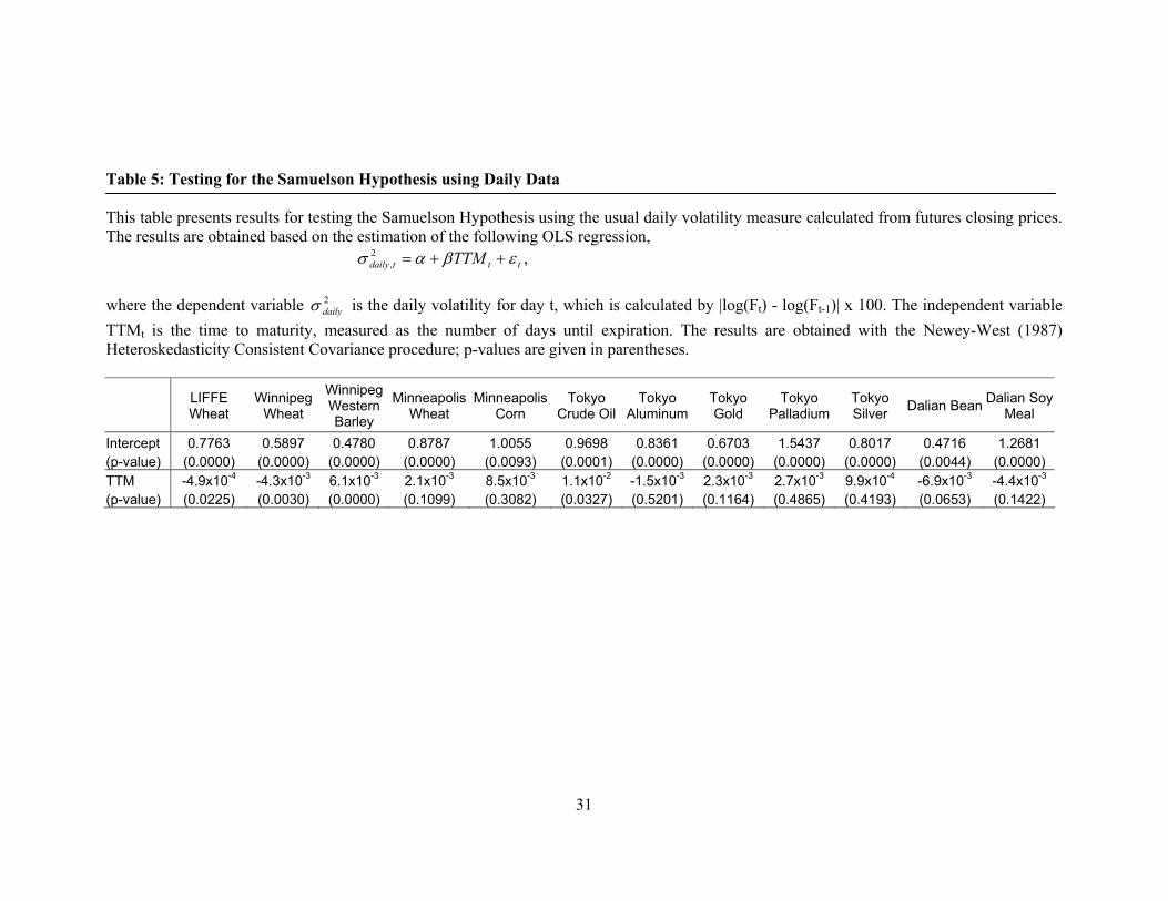
To investigate the Samuelson Hypothesis, the daily volatility measure is also regressed

on time to maturity. The results of these regressions are given in Table 5.


Comparing the results in Table 4 with those in Table 5 gives some interesting insights.

Table 4 and Table 5 show similar results in only eight out of twelve markets: the wheat

markets in LIFFE and WCE; the western barley market in WCE, corn markets in MGEX

and bean markets in DC; and the crude oil, gold and palladium markets in TOCOM.

Inconsistent results between the two tables are observed for other markets. This

inconsistency illustrates the disadvantage of using daily closing prices to calculate daily

volatility. Although this measure of daily volatility is unbiased, it is also an extremely

noisy parameter. Daily realized volatility, which is calculated based on intraday returns

provides a more consistent and efficient measure for daily volatility, as shown in Andersen

and Bollerslev (1998) and Barndorff-Nielsen & Shephard (2001).

In addition, the Samuelson Hypothesis is also tested using the GARCH (Bollerslev, 1986)

and EGARCH (Nelson, 1991) models. As Bollerslev, Chou and Kroner (1992) point out in

14

their survey paper, (G)ARCH-type models are widely used in those studies that deal with

volatility modeling. The characteristic of daily return, as highlighted in Panel B of Table 2,

also provides motivation for the use of the GARCH model in our study. The hypothesis is

examined first with utilizing a GARCH (1,1) model.10 In order to investigate the

Samuelson Hypothesis, the time to maturity variable is included as an exogenous variable

in the conditional variance equation of the GARCH model. The model is specified as

follows:

rt = µ + εt, , εt | Ω t-1 ∼ i.i.d. (0, 2tσ )

tttt TTMδβσαεωσ +++= −−2

12

12 , (2)

where rt is the futures contracts return for day t; TTMt is the number of days to maturity; µ

is constant and εt is the error term process with mean zero and conditional variance 2tσ .

Initially, we estimate the GARCH (1,1) model where the error term follows a normal

distribution. In addition, in order to incorporate the potential leptokurtic distribution of the

error term, we also re-estimate the model using a student t-distribution. If the Samuelson

Hypothesis is supported, the coefficient of the time to maturity variable (δ) should be

negative and statistically significant.

The result of this analysis is given in Table 6. The Samuelson Hypothesis is supported

in the wheat markets in LIFFE, WCE, MGEX, the palladium market in TOCOM and the

soy meal market in DC, as negative and significant coefficients for time to maturity

variables are observed in those markets. For all other markets, the coefficients for time to

maturity variables are insignificantly different from zero. The Ljung-Box statistics for

squared residual Q2(20) shows the non-existence of remaining ARCH effects in ten out of

10 According to Bollerslev (1987) this is the simplest model that performs well in capturing the dynamics

of volatility.

15

twelve markets; remaining ARCH effects exist only in the western barley market in WCE

and the silver market in TOCOM.


Comparing with the results obtained when using the Jonckheere – Terpstra test and

regression analysis, using GARCH (1,1) yields similar results in only six out of twelve

markets. Using the GARCH (1,1) model, the time to maturity variable becomes

insignificant in the western barley market in WCE and the crude oil, aluminium and silver

markets in TOCOM, as opposed to the positive and significant results obtained when using

realized volatility. The time to maturity variable for bean markets in DC now becomes

insignificant at the 10% level and that for the palladium market in Tokyo becomes negative

and significant, as opposed to the insignificant results obtained with the OLS regression

with realized volatility. We also re-estimate the GARCH (1,1) model with the error term

allowed to follow a student t-distribution, which might arguably be better for capturing the

leptokurtic distribution nature of the error term. The result for this estimation is given in

Table 7.


Comparing the results of Table 7 with that of Table 6, allowing the error term to follow

a student t-distribution does improve the estimation. The remaining ARCH effects are

eliminated for the western barley market in WCE and the result of the Samuelson

Hypothesis for this market is consistent with the result when using the OLS regression with

realized volatility. However, the ARCH effect still exists for the silver market in Tokyo,

which explains this market’s inconsistent result compared to the results when using realized

volatility. Beside the silver market, inconsistent results between the GARCH (1,1) model

16

and the OLS regression with realized volatility still exist for aluminium and crude oil

markets in TOCOM and for the bean market in DC.

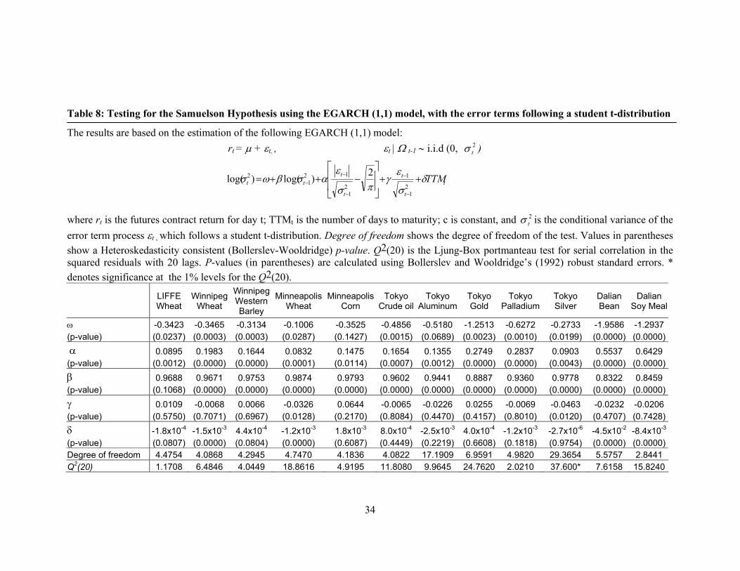
In order to capture any potential “leverage effect”, the EGARCH model of Nelson

(1991) is also utilized to investigate the Samuelson Hypothesis, as follows,

rt = µ + εt, , εt | Ω t-1 ∼ i.i.d. (0, 2tσ )

t

t

t

t

ttt TTMδ

σ

εγ

πσ

εασβωσ ++

−++=

−

−

−

−−

21

1

21

121

2 2)log()log( , (3)

The error term is assumed to follow a student t-distribution. A negative and significant

coefficient for the coefficient γ provides evidence of the existence of a “leverage effect”.

The results of the estimation are given in Table 8. Negative and significant coefficients

for time to maturity variables are observed in wheat markets in LIFFE, WCE, MGEX and

bean and soy meal markets in DC. These results are similar with the results obtained when

using the OLS regression with realized volatility. Consistent results between the EGARCH

(1,1) model and the OLS regression with realized volatility are also found in the western

barley market in WCE, the corn market in MGEX, and the gold and palladium markets in

TOCOM. The silver, crude oil and aluminium markets in TOCOM still give inconsistent

results with the results when using the OLS regression with realized volatility. Remaining

ARCH effects do not exist in eleven out of twelve markets; only the silver market still

possesses the ARCH effect after estimating with the EGARCH (1,1) model. This helps

explain the inconsistency between the results of the Samuelson Hypothesis, which uses the

EGARCH (1,1) model, and the results based on regression with realized volatility for silver

markets. For the other two markets (crude oil and aluminium markets in Tokyo) the

difference in results with realized volatility might be due to the fact that the returns

modelled by the GARCH and EGARCH models in this study are daily returns, as opposed

17

to the use of intraday returns in realized volatility. In fact, for the aluminium market, the

GARCH and EGARCH models give similar results to those in Table 5, when the absolute

daily return is used as a measure for the daily volatility. With regards to the “leverage

effect”, this effect exists in only two out of twelve markets (the silver market in Tokyo and

the wheat market in Minneapolis). For the other ten markets, the coefficient γ is statistically

indistinguishable from zero, indicating the non-existence of the “leverage effect”.


In general, using various methodologies, this study provides mixed support for the

Samuelson Hypothesis. The hypothesis is supported in the wheat markets in LIFFE,

MGEX and WCE and in the bean and soy meal markets in DC. No maturity effect exists

for the other two agricultural futures (corn markets in Minneapolis and western barley

markets in Winnipeg), for the metals futures (aluminium, gold, silver and palladium

markets in Tokyo) and the energy futures (crude oil) in Tokyo.

4.3 The “Negative Covariance” Hypothesis

This hypothesis examines the “negative covariance” hypothesis proposed by

Bessembinder et al. (1996). This hypothesis states that the Samuelson Hypothesis is more

likely to be supported in those markets that exhibit a negative covariance between the spot

prices changes and changes in net carry costs. Because spot prices for commodity futures

are not generally available, this study follows Fama and French (1988) in using futures

prices in the contract month as the proxy for spot prices. Following Bessembinder et al.

(1995), the net carry cost is the difference between the natural logarithm of futures and spot

prices, weighted by the time to maturity, as specified below,

c j, t = (f j,t – s j, t) / TTMt

18

where f j,t is the natural logarithm of the price for futures contract j on day t; c j, t is the net

carry cost for contract j in day t; s j, t is a natural logarithm of the spot price at time t and

TTMt is the number of days to maturity.

The covariance between changes in spot prices and changes in net carry costs is then

estimated as in the following regression,

∆c j, t = α0 + α1 ∆ s j, t + εt , (4)

where ∆c j, t and ∆sj, t are the changes in net carry costs and changes in spot prices,

respectively.11

If the maturity effect tends to be stronger for markets that have negative covariance (α1 <0),

the Bessembinder et al. (1996) hypothesis is supported. The results of these regressions are

given in Table 9.


The results in Table 9 show a negative covariance between spot price changes and changes

in net carry costs for all twelve markets examined in this study. Ten out of the twelve

covariances are significantly different from zero, with the exception of aluminum and gold

markets in TOCOM. For wheat markets in LIFFE, WCE, MGEX and bean and soy meal

markets in DC, the estimates of the covariance are uniformly negative, significant and large

in absolute magnitude. The estimates of the covariance between changes in spot prices and

changes in net carry costs for western barley, corn, crude oil, palladium and silver markets

are negative and, while significant, are in an order of absolute magnitude smaller than the

estimates for wheat, bean and soy meal markets. These results are consistent with

Bessembinder et al. (1995), who find larger estimates of the covariance between net carry

costs and spot prices in agricultural futures in comparison to metal futures. Based on these

11 We follow Bessembinder et al. (1995) and estimate this regression using first differences. In addition,

to facilitate the comparison of coefficient estimates, we divide each price series by its own mean. The net carry cost is also multiplied by 25,000 and hence it can be interpreted as an annualized percentage.

19

estimates, we anticipate that the Samuelson Hypothesis will be strongly supported for

wheat futures in LIFFE, Winnipeg and Minneapolis and for bean and soy meal futures in

Dalian. Little or no support for the Samuelson Hypothesis is anticipated for western barley,

corn, crude oil, palladium, silver, aluminum and gold futures. The results obtained when

investigating the Samuelson Hypothesis in section 4.2 confirm this prediction. As expected,

the Samuelson Hypothesis is supported in wheat markets in LIFFE, WCE and MGEX and

in bean and soy meal markets in DC. No evidence of the Samuelson Hypothesis is found

for other markets. Overall, consistent with Bessembinder et al. (1996), these results provide

support for the “negative covariance” hypothesis. This hypothesis works well in explaining

the difference in the degree of support for the Samuelson Hypothesis in the twelve markets

examined in this study.

4.4 The “State Variable” Hypothesis

Under the “state variable” hypothesis, information flow is the main determinant of time

patterns for the futures price volatility. The Samuelson Hypothesis is viewed as a special

case where the information flow is greater as the delivery date approaches. Following

Bessembinder et al. (1996), spot price volatility is used as the proxy for information flow.

In order to investigate the effect of information flow, firstly daily futures realized volatility

is regressed on days to maturity,

RVt = α + β TTMt + εt (5)

Secondly, the spot price volatility (Vola(S j,t)) is also included as a control variable in the

regression equation

RVt = α + β TTMt + φ Vola(S j,t) + εt , (6)

20

If the “negative covariance” condition is the most significant determinant of the Samuelson

hypothesis, as suggested by Bessembinder et al. (1996), the coefficient of the days to

maturity variable (β) should remain negative and significant despite the inclusion of the

spot price volatility variable.

The results of this investigation of the information flow effects are given in Table 10.

Consistent with the findings of previous studies12, estimated coefficients for the spot price

volatility are uniformly positive and each of these coefficients is significant. The spot price

volatility appears to have explanatory power over the futures price volatility. More

importantly, consistent with the findings of Bessembinder et al. (1996), the addition of spot

price volatility has little affect on the estimates of parameters associated with time to

maturity. The estimates of the parameters for the time to maturity variable are largely

unchanged. The main effect of the inclusion of spot price volatility is the reduction in

standard errors, so that now the time to maturity variable becomes significant for the

aluminum market in TOCOM. The Samuelson Hypothesis is still supported for wheat

markets in LIFFE, WCE, MGEX and bean and soy meal markets in DC. For the remaining

six markets, similar results regarding the Samuelson Hypothesis are obtained regardless of

the inclusion of spot price volatility.

Overall, consistent with Bessembinder et al. (1996), we conclude that although the

information flow plays a role in explaining futures price volatility, it is not the main

determinant for the success of the Samuelson Hypothesis. Together with the results of

Hypothesis 2, it is concluded that the information flow does not dominate the “negative

covariance” condition in explaining the maturity effect.

12 See for example Bessembinder et al. (1996) and Allen & Cruickshank (2000).

21


5. Conclusion

The main objective of the study is to examine the Samuelson Hypothesis in commodity

futures contracts. Investigating 336 commodity futures contracts from twelve futures

markets in five futures exchanges, this study, for the first time, provides high-frequency

data evidence of the Samuelson Hypothesis for commodity futures contracts. Utilizing the

Jonckheere – Terpstra Test, OLS regressions with realized volatility and various GARCH

models, the study provides mixed evidence regarding support for the Samuelson

Hypothesis. In general, agricultural futures provide stronger support for the Samuelson

Hypothesis than metals futures. Evidence supporting the Samuelson Hypothesis is found in

wheat markets in LIFFE, WCE, MGEX and bean and soy meal markets in DC. The

Samuelson Hypothesis is not supported in the other seven markets (western barley in WCE;

corn in MGEX; aluminum, crude oil, gold, silver, and palladium in TOCOM).

In addition, the study also provides support for the “negative covariance” hypothesis of

Bessembinder et al. (1996). Negative and significant covariances between spot price

changes and changes in net carry costs are observed for ten out of twelve markets examined

in this study. The estimates for these covariances are uniformly negative, significant and

large in absolute magnitude for wheat markets in LIFFE, WCE and MGEX and in bean and

soy meal markets in DC. For the other markets, the covariance is either insignificantly

different from zero or negative but in the order of a smaller absolute magnitude. This helps

explain the strong support for the Samuelson Hypothesis in wheat, bean and soy meal

futures as opposed to the limited support for the Samuelson Hypothesis in other futures.

22

In contrast to the argument of the “state variable” hypothesis, information flow does not

appear to be the main determinant of support for the Samuelson Hypothesis. The empirical

evidence regarding the Samuelson Hypothesis remains almost identical, regardless of the

inclusion or omission of information flow in the regression. It is therefore concluded that

for the twelve markets examined in this study, the information flow does not dominate the

“negative covariance” condition in explaining the maturity effect, as is suggested by the

“negative covariance” hypothesis.

23

References

Allen, D. E., Cruickshank, S. N., 2000. Empirical testing of the Samuelson Hypothesis: An

application to futures markets in Australia, Singapore and the UK. Working paper,

School of Finance and Business Economics, Edith Cowan University.

Andersen, T. G., Bollerslev, T., 1998. Answering the skeptics: Yes, standard volatility

models do provide accurate forecasts. International Economic Review 39(4), 885--905.

Anderson, R. W., 1985. Some Determinants of the Volatility of Futures Prices. Journal of

Futures Markets 5(3), 331--348.

Anderson, R. W., Danthine, J., 1983. The Time Pattern of Hedging and the Volatility of

Futures Prices. Review of Economic Studies 50, 249--266.

Areal, N.M.P.C., Taylor, S. J., 2002. The Realized Volatility of FTSE-100 Future Prices.

Journal of Futures Markets 22(7), 627--648.

Barndorff-Niesen, O. E., Shephard, N., 2001. Non-Gaussian Ornstein – Uhlenbeck – based

models and some of their uses in financial economics. Journal of the Royal Statistical

Society, Series B 63, 167--241.

Barnhill, T. M., Jordan, J. V., Seale, W. E., 1987. Maturity and Refunding Effects on

Treasury-Bond Futures Price Variance. Journal of Financial Research 10, 121--131.

Bessembinder, H., Coughenour, J. F., Seguin, P. J., Smoller, M. M., 1995. Mean Reversion

in Equilibrium Asset Prices: Evidence from the Futures Term Structure. Journal of

Finance 50, 361--375.

Bessembinder, H., Coughenour, J. F., Seguin, P. J., Smoller, M. M., 1996. Is here a Term

Structure of Futures Volatilities? Reevaluating the Samuelson Hypothesis. Journal of

Derivatives 4, 45--58.

Board, J., Sutcliffe, C., 1990. Information, Volatility, Volume, And Maturity: An

Investigation Of Stock Index Futures. Review of Futures Markets 9(3), 532--549.

24

Bollerslev, T., 1986. Generalized Autoregressive Conditional Heteroscedasticity. Journal of

Econometrics 31, 307--326.

Bollerslev, T., 1987. A Conditionally Heteroskedastic Time Series Model for Speculative

Prices and Rates of Return. The Review of Econometrics and Statistics 69, 542--547.

Bollerslev, T., Chou, R.Y., Kroner, K.F., 1992. ARCH Modeling in Finance: A Review of

the Theory and Empirical Evidence. Journal of Econometrics 52, 5--59.

Bollerslev, T., Wooldridge, J.M., 1992. Quasi-Maximum Likelihood Estimation and

Inference in Dynamic Models with Time-Varying Covariances. Econometric Reviews

11(2), 143--172.

Chen, Y. J., Duan, J. C., Hung, M. W., 1999. Volatility and Maturity Effects in the Nikkei

Index Futures. Journal of Futures Markets 19(8), 895--909.

Dusak-Miller, K., 1979. The Relation Between Volatility and Maturity in Futures

Contracts. Leuthold, R. M. (ed.) Commodity Markets and Futures Prices, Chicago

Mercantile Exchange, 25--36.

Fama, E., French, K., 1988. Business Cycles and the Behaviour of Metals Prices. Journal of

Finance 43, 1075--1093.

Galloway, T. M., Kolb, R. W., 1996. Futures Prices and the Maturity Effect. Journal of

Futures Markets 16(7), 809--828.

Grammatikos, T., Saunders, A., 1986. Futures Price Variability: A Test of Maturity and

Volume Effects. Journal of Business 59, 319--330.

Jonckheere, A. R., 1954. A distribution-free-k-sample test against ordered alternatives.

Biometrika 41 (1-2), 133--145.

Kenyon, D., Kenneth, K., Jordan, J., Seale, W., McCabe, N., 1987. Factors Affecting

Agricultural Futures Price Variance. Journal of Futures Markets 7(1), 73--91.

25

Khoury, N., Yourougou, P., 1993. Determinants of Agricultural Futures Prices Volatilities:

Evidence from Winnipeg Commodity Exchange. Journal of Futures Markets 13(4),

345--56.

Milonas, N., 1986. Price Variability and the Maturity Effect in Futures Markets. Journal of

Futures Markets 6, 443--460.

Nelson, D.B., 1991. Conditional Heteroskedasticity in Asset Returns: A New Approach.

Econometrica 59, 347--370.

Newey, W., West, K., 1987. Hypothesis testing with efficient method of moment

estimation. International Economic Review 28, 777--787.

Roll, R., 1984. A simple implicit measure of the effective bid-ask spread in an efficient

market. Journal of Finance 39, 1127--1139.

Rutledge, D.J.S., 1976. A Note on the Variability of Futures Prices. Review of Economics

and Statistics 58, 118--120.

Samuelson, P. A., 1965. Proof that Properly Anticipated Prices Fluctuate Randomly.

Industrial Management Review 6, 41--49.

Terpstra, T. J., 1954. The asymptotic normality and consistency of Kendall’s test against

trend when ties are present in one ranking. Indagationes Mathematicae 14, 327--333

Thomakos, D. D., Wang, T., 2003. Realized Volatility in the Futures Market. Journal of

Empirical Finance 10, 321--353.

26

Table 1: Basic Facts of Futures Contracts Studied This table outlines basic facts of the commodity futures investigated in this study. All data has been retrieved from SIRCA. Expiration month is a numerical representation of the month in which each contract expires ( 1 = January; 2 = February; 3 = March and so on). Overall, the study examines 336 futures contracts of twelve commodities in five futures exchanges.

Commodity Futures Exchange Sample Period Number of contracts Expiration Month Wheat LIFFE 2-Jan-1996 to 30-Oct-2000 25 1,3,5,7,9,11 Wheat Winnipeg 2-Jan-1996 to 31-Oct-2003 40 3,5,7,10,12

Western Barley Winnipeg 2-Jan-1996 to 31-Oct-2003 40 3,5,7,10,12 Wheat Minneapolis 2-Jan-1996 to 31-Oct-2003 41 3,5,7,9,12 Corn Minneapolis 15-Feb-2002 to 31-Oct-2003 21 1,2,3,4,5,6,7,8,9,10,11,12

Aluminum Tokyo 1-May-2000 to 31-Oct-2003 42 1,2,3,4,5,6,7,8,9,10,11,12 Crude Oil Tokyo 11-Sep-2000 to 31-Oct-2003 24 1,2,3,4,5,6,7,8,9,10,11,12

Gold Tokyo 1-Sep-1999 to 31-Oct-2003 26 2,4,6,8,10,12 Silver Tokyo 1-Sep-1999 to 31-Oct-2003 26 2,4,6,8,10,12

Palladium Tokyo 1-Sep-1999 to 31-Oct-2003 26 2,4,6,8,10,12 Bean Dalian 2-Jan-2003 to 31-Oct-2003 5 1,3,5,7,9,11

Soy Meal Dalian 1-Oct-2000 to 31-Oct-2003 20 1,3,5,7,9,11

27

Table 2: Panel A: Descriptive statistics for Daily Realised Volatility This table provides descriptive statistics for daily realised volatility for various commodities in five futures exchanges: LIFFE, WCE, MGEX, TOCOM, and DC. The daily realised volatility is calculated as the sum of squared five-minute interval returns, specified as follows, RVj,t =

∑=

n

iitjr

1

2,, )( . This table also reports the Ljung-Box statistics for measures of autocorrelation. Q(20) is the Ljung-Box statistics for 20th order.

Jarque-Bera is the Jarque-Bera statistics for testing the null hypothesis of a normal distribution. ADF is the Augmented Dickey-Fuller test for unit root. The number of lags chosen is 4. The critical value for rejection of the unit root hypothesis is –3.4338 (at 1% level). * denotes significance at the 1% level.

LIFFE Wheat

Winnipeg Wheat

Winnipeg Western Barley

Minneapolis Wheat

Minneapolis Corn

Tokyo Crude Oil

Tokyo Aluminum Tokyo Gold Tokyo

PalladiumTokyo Silver

Dalian Bean

Dalian Soy Meal

Mean 3.3x10-4 1.5x10-4 2.5x10-4 1.5x10-4 2.1x10-3 4.9x10-4 2.5x10-4 1.8x10-4 5.3x10-4 2.9x10-4 1.5x10-4 1.8x10-3

Median 2.5x10-4 1.3x10-4 1.9x10-4 1.1x10-4 7.7x10-4 2.8x10-4 2.2x10-4 1.2x10-4 2.5x10-4 2.3x10-4 6.5x10-5 6.3x10-4

Std Dev 2.9x10-4 1.1x10-4 2.1x10-4 1.6x10-4 3.8x10-3 6.1x10-4 1.6x10-4 2.1x10-4 7.9x10-4 2.4x10-4 2.5x10-4 2.7x10-3

Skewness 2.35 1.81 3.12 3.90 4.06 3.02 1.29 3.78 3.36 1.91 3.88 2.90Kurtosis 10.40 10.75 18.82 28.92 21.71 15.14 5.11 22.13 17.94 8.18 20.50 14.62

ADF -9.38 -14.96 -13.55 -9.99 -7.14 -6.61 -10.52 -9.45 -9.08 -10.92 -3.67 -7.65Q(20) 538.2* 348.4* 707.4* 2326.0* 202.9* 255.5* 56.9* 734.4* 225.6* 114.2* 45.7* 490.5*

Jarque-Bera 3605.5* 5507.8* 23059.3* 57745.6* 6446.2* 3935.2* 388.7* 17664.8* 9099.2* 1733.8* 2870.3* 5148.1*

28

Table 2: Panel B: Descriptive Statistics for Daily Returns This table provides descriptive statistics for daily returns for various commodities in five futures exchanges: LIFFE, Minneapolis, Tokyo, Winnipeg and Dalian. Daily returns are calculated as the log difference of futures closing prices, specified as log(Ft) – log(Ft-1). This table also reports the Ljung-Box statistics for measures of autocorrelation. Q(20) is the Ljung-Box statistics for the 20th order. Jarque-Bera is the Jarque-Bera statistics for testing the null hypothesis of a normal distribution. ADF is the Augmented Dickey-Fuller test for unit roots. The number of lags chosen is 4. The critical value for rejection of the unit root hypothesis is –3.4338 (at the 1% level). All the Jarque-Bera statistics are significant at the 1% level.

LIFFE Wheat

Winnipeg Wheat


Minneapolis Wheat

Minneapolis Corn

Tokyo Crude Oil

Tokyo Aluminum

Tokyo Gold

Tokyo Palladium

Tokyo Silver

Dalian Bean

Dalian Soy Meal

Mean -6.2x10-4 -2.5x10-4 -1.5x10-4 -1.4x10-4 5.2x10-4 -5.7x10-5 3.6x10-5 4.1x10-4 -6.5x10-4 -3.2x10-5 1.1x10-3 7.4x10-4

Median -7.0x10-4 0.00 0.00 -7.7x10-4 0.00 9.6x10-4 -5.5x10-4 0.00 -7.2x10-4 0.00 3.8x10-4 5.9x10-4

Std Dev 0.01 0.01 0.01 0.01 0.02 0.02 0.01 0.01 0.02 0.01 0.01 0.02Skewness -3.26 -0.89 -1.79 0.39 0.27 -0.22 0.31 0.73 0.66 -0.12 -0.05 0.35Kurtosis 51.74 22.63 29.81 12.51 7.73 3.50 3.90 8.59 10.38 3.80 5.00 9.79ADF -25.81 -41.20 -42.79 -40.74 -22.47 -22.07 -30.49 -33.25 -23.19 -36.65 -11.74 -33.69Q(20) 20.06 10.19 34.05** 37.37** 37.14** 15.89 20.79 31.59** 104.9* 44.6* 20.53 65.3*Jarque -Bera 113367.4* 29242.9* 58308.2* 7168.1* 351.1* 9.72* 41.9* 1390.2* 1902.9* 29.2* 31.5* 1421.9*

29

Table 3: Testing for the Samuelson Hypothesis using the Jonckheere – Terpstra test This table presents results of testing for the Samuelson Hypothesis using the Jonckheere – Terpstra test of ordered alternatives. For each commodity, the Jonckheere – Terpstra test is applied to a period of time when a number of contracts with different maturities are traded. The Jonckheere – Terpstra test is then used to test for the null hypothesis of equal volatility of all contracts against the alternative hypothesis where higher volatility is observed for contracts closer to maturity. The null and the ordered alternate forms can be shown as follows:

H0 : 222

21 ... kσσσ ===

H1: 222

21 ... kσσσ >>>

where k is the number of contracts and 21σ is the volatility of the contract closest to maturity, 2

2σ is the volatility of the contract second closest to maturity and so on. The test statistics (JT statistics) follows the standard normal distribution; p-values are given in parentheses.

LIFFE Wheat

Winnipeg Wheat


Minneapolis Wheat

Minneapolis Corn

Tokyo Crude Oil

Tokyo Aluminum

Tokyo Gold

Tokyo Palladium

Tokyo Silver

Dalian Bean

Dalian Soy Meal

JT statistic 12.48 9.94 1.16 12.79 0.73 1.27 0.38 1.09 1.13 1.24 7.7 1.45 (p-value) (0.00) (0.00) (0.12) (0.00) (0.23) (0.11) (0.35) (0.14) (0.13) (0.11) (0.00 (0.07)

30

Table 4: Testing for the Samuelson Hypothesis using Realised Volatility This table presents results for testing the Samuelson Hypothesis using daily realised volatility. The results are based on the estimation of the following OLS regression,

RVt = α + β TTMt + εt, where the dependent variable (RVt) is the realised volatility for day t, which is the sum of squared five-minute interval returns in day t. The independent variable TTMt is the time to maturity, measured as the number of days until expiration. The results are obtained with the Newey-West (1987) Heteroskedasticity Consistent Covariance procedure; p-values are given in parentheses.

LIFFE Wheat

Winnipeg Wheat


Minneapolis Wheat

Minneapolis Corn

Tokyo crude Oil

Tokyo Aluminum

Tokyo Gold

Tokyo Palladium

Tokyo Silver Dalian Bean Dalian Soy

Meal

Intercept 4.1x10-4 1.7x10-4 1.8x10-4 1.7x10-4 9.0x10-4 1.3x10-4 2.0x10-4 1.7x10-4 4.8x10-4 2.4x10-4 2.9x10-4 3.8x10-3 (p-value) (0.0000) (0.0000) (0.0000) (0.0000) (0.3207) (0.3514) (0.0000) (0.0000) (0.0000) (0.0000) (0.0001) (0.0000) TTM -1.2x10-6 -2.9x10-7 1.2x10-6 -3.3x10-7 2.5x10-5 8.2x10-6 1.1x10-6 1.1x10-7 8.7x10-7 8.7x10-7 -3.0x10-6 -4.6x10-5 (p-value) (0.0000) (0.0148) (0.0000) (0.0579) (0.2338) (0.0104) (0.0871) (0.7672) (0.5711) (0.0413) (0.0247) (0.0000)

31

Table 5: Testing for the Samuelson Hypothesis using Daily Data This table presents results for testing the Samuelson Hypothesis using the usual daily volatility measure calculated from futures closing prices. The results are obtained based on the estimation of the following OLS regression,

tttdaily TTM εβασ ++=2, ,

where the dependent variable 2

dailyσ is the daily volatility for day t, which is calculated by |log(Ft) - log(Ft-1)| x 100. The independent variable TTMt is the time to maturity, measured as the number of days until expiration. The results are obtained with the Newey-West (1987) Heteroskedasticity Consistent Covariance procedure; p-values are given in parentheses.

LIFFE Wheat

Winnipeg Wheat


Minneapolis Wheat

Minneapolis Corn

Tokyo Crude Oil

Tokyo Aluminum

Tokyo Gold

Tokyo Palladium

Tokyo Silver Dalian Bean Dalian Soy

Meal

Intercept 0.7763 0.5897 0.4780 0.8787 1.0055 0.9698 0.8361 0.6703 1.5437 0.8017 0.4716 1.2681 (p-value) (0.0000) (0.0000) (0.0000) (0.0000) (0.0093) (0.0001) (0.0000) (0.0000) (0.0000) (0.0000) (0.0044) (0.0000) TTM -4.9x10-4 -4.3x10-3 6.1x10-3 2.1x10-3 8.5x10-3 1.1x10-2 -1.5x10-3 2.3x10-3 2.7x10-3 9.9x10-4 -6.9x10-3 -4.4x10-3 (p-value) (0.0225) (0.0030) (0.0000) (0.1099) (0.3082) (0.0327) (0.5201) (0.1164) (0.4865) (0.4193) (0.0653) (0.1422)

32

Table 6: Testing the Samuelson Hypothesis using a GARCH (1,1) model with error terms following a normal distribution

The results are based on the estimation of the following GARCH (1,1) model: rt = µ + εt, , εt | Ω t-1 ∼ i.i.d (0, 2

tσ )


12

12

where rt is the futures contract return for day t; TTMt is the number of days to maturity; c is constant and 2

tσ is the conditional variance of the

error term process εt , which follows a normal distribution. Q2(20) is the Ljung-Box portmanteau test for serial correlation in the squared residuals with 20 lags. P-values (in parentheses) are calculated using Bollerslev and Wooldridge’s (1992) robust standard errors. *, ** denotes significance at the 1% and 5% levels for the Q2(20) respectively.

LIFFE Wheat

Winnipeg Wheat


Minneapolis Wheat

Minneapolis Corn

Tokyo Crude Oil

Tokyo Aluminum

Tokyo Gold

Tokyo Palladium

Tokyo Silver

Dalian Bean

Dalian Soy Meal

ω 0.0001 2.15x10-5 9.39x10-7 1.84x10-5 1.23x10-5 -1.53x10-6 1.03x10-5 1.63x10-5 5.55x10-5 5.80x10-6 4.33x10-5 9.01x10-5

(p-value) (0.0011) (0.0000) (0.9601) (0.0000) (0.4675) (0.8316) (0.0918) (0.0179) (0.0002) (0.1227) (0.0107) (0.0000) α 0.1500 0.1560 0.2657 0.0310 0.0486 0.0813 0.0699 0.1644 0.1046 0.0651 0.0604 0.2182 (p-value) (0.0272) (0.0021) (0.0003) (0.0002) (0.0840) (0.0093) (0.0503) (0.0104) (0.0037) (0.0028) (0.3799) (0.0005) β 0.6000 0.8051 0.1499 0.9466 0.9300 0.8821 0.8572 0.6882 0.8723 0.9005 0.7972 0.6816 (p-value) (0.0000) (0.0000) (0.6524) (0.0000) (0.0000) (0.0000) (0.0000) (0.0000) (0.0000) (0.0000) (0.0000) (0.0000) δ -9.3x10-8 -2.3x10-7 1.6x10-6 -2.4x10-7 -3.2x10-8 3.2x10-7 -7.5x10-8 1.2x10-8 -6.6x10-7 -3.2x10-8 -6.0x10-7 -1.3x10-6 (p-value) (0.0000) (0.0448) (0.1941) (0.0121) (0.9288) (0.1062) (0.6765) (0.9261) (0.0117) (0.7576) (0.1095) (0.0000) Q2(20) 0.7532 8.6849 32.42** 13.1460 7.9828 11.7310 9.2937 20.6300 1.7243 38.2750* 13.4500 8.1119

33

Table 7: Testing the Samuelson Hypothesis using a GARCH (1,1) model with error terms following a student t-distribution

The results are based on the estimation of the following GARCH (1,1) model: rt = µ + εt, , εt | Ω t-1 ∼ i.i.d (0, 2

tσ )


12

12

where rt is the futures contract return for day t; TTMt is the number of days to maturity; c is constant and 2

tσ is the conditional variance of the

error term process εt , which follows a student t-distribution.. Degree of freedom shows the degree of freedom of the test. . Q2(20) is the Ljung-Box portmanteau test for serial correlation in the squared residuals with 20 lags. P-values (in parentheses) are calculated using Bollerslev and Wooldridge’s (1992) robust standard errors. * denotes significance at the 1% for the Q2(20).

LIFFE Wheat

Winnipeg Wheat


Minneapolis Wheat

Minneapolis Corn

Tokyo Crude Oil

Tokyo Aluminum

Tokyo Gold

Tokyo Palladium

Tokyo Silver

Dalian Bean

Dalian Soy Meal

ω 1.12x10-4 1.47x10-5 7.64x10-6 1.39x10-5 -5.41x10-7 -1.56x10-6 1.16x10-5 1.04x10-5 8.17x10-5 5.42x10-6 4.53x10-5 1.18x10-4

(p-value) (0.0095) (0.0000) (0.0003) (0.0000) (0.9887) (0.9368) (0.2061) (0.0948) (0.0092) (0.1672) (0.4022) (0.0129) α 0.1499 0.0905 0.0700 0.0347 0.0667 0.0813 0.0636 0.1379 0.1909 0.0594 0.4774 0.6855 (p-value) (0.042) (0.0000) (0.0000) (0.0001) (0.0277) (0.00110 (0.0061) (0.0000) (0.0001) (0.0024) (0.1704) (0.0144) β 0.5999 0.8726 0.9086 0.9447 0.9237 0.8821 0.8750 0.7421 0.7620 0.9077 -0.0892 0.5029 (p-value) (0.0001) (0.0000) (0.0000) (0.0000) (0.0000) (0.0000) (0.0000) (0.0000) (0.0000) (0.0000) (0.4957) (0.0000) δ -8.3x10-8 -1.5x10-7 7.0x10-8 -1.7x10-7 1.7x10-7 3.2x10-7 -1.3x10-7 6.1x10-8 -7.8x10-7 -2.8x10-8 1.7x10-6 -1.6x10-6 (p-value) (0.0000) (0.0000) (0.0127) (0.0000) (0.8400) (0.4775) (0.4857) (0.5065) (0.0789) (0.6419) (0.1863) (0.0214) Degree of freedom 20.000 3.9053 4.2571 4.4982 4.0598 5.5869 17.5977 7.1364 4.9010 24.9408 3.0892 2.7219 Q2(20) 0.7395 7.3140 4.9033 12.8850 5.8077 11.7330 9.0623 22.2640 1.7981 38.487* 4.2252 11.3810

34

Table 8: Testing for the Samuelson Hypothesis using the EGARCH (1,1) model, with the error terms following a student t-distribution

The results are based on the estimation of the following EGARCH (1,1) model: rt = µ + εt, , εt | Ω t-1 ∼ i.i.d (0, 2

tσ )

t

t

t

t

ttt TTMδ

σ

εγ

πσ

εασβωσ ++

−++=

−

−

−

−−

21

1

21

121

2 2)log()log(

where rt is the futures contract return for day t; TTMt is the number of days to maturity; c is constant, and 2

tσ is the conditional variance of the error term process εt , which follows a student t-distribution. Degree of freedom shows the degree of freedom of the test. Values in parentheses show a Heteroskedasticity consistent (Bollerslev-Wooldridge) p-value. Q2(20) is the Ljung-Box portmanteau test for serial correlation in the squared residuals with 20 lags. P-values (in parentheses) are calculated using Bollerslev and Wooldridge’s (1992) robust standard errors. * denotes significance at the 1% levels for the Q2(20).

LIFFE Wheat

Winnipeg Wheat


Minneapolis Wheat

Minneapolis Corn

Tokyo Crude oil

Tokyo Aluminum

Tokyo Gold

Tokyo Palladium

Tokyo Silver

Dalian Bean

Dalian Soy Meal

ω -0.3423 -0.3465 -0.3134 -0.1006 -0.3525 -0.4856 -0.5180 -1.2513 -0.6272 -0.2733 -1.9586 -1.2937(p-value) (0.0237) (0.0003) (0.0003) (0.0287) (0.1427) (0.0015) (0.0689) (0.0023) (0.0010) (0.0199) (0.0000) (0.0000) α 0.0895 0.1983 0.1644 0.0832 0.1475 0.1654 0.1355 0.2749 0.2837 0.0903 0.5537 0.6429 (p-value) (0.0012) (0.0000) (0.0000) (0.0001) (0.0114) (0.0007) (0.0012) (0.0000) (0.0000) (0.0043) (0.0000) (0.0000)β 0.9688 0.9671 0.9753 0.9874 0.9793 0.9602 0.9441 0.8887 0.9360 0.9778 0.8322 0.8459 (p-value) (0.1068) (0.0000) (0.0000) (0.0000) (0.0000) (0.0000) (0.0000) (0.0000) (0.0000) (0.0000) (0.0000) (0.0000)γ 0.0109 -0.0068 0.0066 -0.0326 0.0644 -0.0065 -0.0226 0.0255 -0.0069 -0.0463 -0.0232 -0.0206(p-value) (0.5750) (0.7071) (0.6967) (0.0128) (0.2170) (0.8084) (0.4470) (0.4157) (0.8010) (0.0120) (0.4707) (0.7428)δ -1.8x10-4 -1.5x10-3 4.4x10-4 -1.2x10-3 1.8x10-3 8.0x10-4 -2.5x10-3 4.0x10-4 -1.2x10-3 -2.7x10-6 -4.5x10-2 -8.4x10-3

(p-value) (0.0807) (0.0000) (0.0804) (0.0000) (0.6087) (0.4449) (0.2219) (0.6608) (0.1818) (0.9754) (0.0000) (0.0000)Degree of freedom 4.4754 4.0868 4.2945 4.7470 4.1836 4.0822 17.1909 6.9591 4.9820 29.3654 5.5757 2.8441 Q2(20) 1.1708 6.4846 4.0449 18.8616 4.9195 11.8080 9.9645 24.7620 2.0210 37.600* 7.6158 15.8240

35

Table 9: Testing for the covariance between spot prices and net carry costs This table presents results for testing for the covariance between spot prices and net carry costs. The results are obtained from the following regression, ∆c j, t = α0 + α1 ∆s j, t + εt

where ∆s j, t is the change in spot prices at time t and ∆cj,t is the change in net carry costs for contract j at day t, which is defined as,

c j, t = (f j,t – s j, t) / TTMt where f j,t is the natural logarithm of the price for futures contract j on day t. The regressions are estimated in first differences and the price series are scaled by dividing by their own means. The dependent variables are multiplied by 25,000 and can be regarded as a yearly percentage. The results are obtained with the Newey-West (1987) Heteroskedasticity Consistent Covariance matrix procedure; p-values are given in parentheses.

LIFFE Wheat

Winnipeg Wheat


Mineapolis Wheat

Mineapolis Corn

Tokyo Crude Oil

Tokyo Aluminum

Tokyo Gold

Tokyo Palladium

Tokyo Silver

Dalian Bean

Dalian SoyMeal

Intercept -0.4220 -0.0796 -0.0874 -0.0584 0.0913 -0.0674 1002.6660 0.0172 -0.2267 -0.0051 -11.5926 0.3630 (p-value) (0.1623) (0.8341) (0.7774) (0.7926) (0.8521) (0.8124) (0.5891) (0.8027) (0.6761) (0.9706) (0.4630) (0.5903) Spot price -331.4188 -196.4336 -89.7841 -153.4626 -59.7514 -47.1837 -1.6272 -12.9716 -66.9697 -65.5112 -382.6900 -236.4270(p-value) (0.0000) (0.0008) (0.0004) (0.0045) (0.0000) (0.0199) (0.8655) (0.2197) (0.0399) (0.0000) (0.0381) (0.0000)

36

Table 10: The effect of information flow when spot price volatility is used as its proxy This table examines the effect of information flows as suggested by the “state-variable” hypothesis. In order to examine the information flow effect, daily futures realised volatility is firstly regressed on time to maturity RVt = α + β TTMt + εt , then on time to maturity and spot price volatility RVt = α + βTTMt + φVola(Sj,t) + εt. These regressions are performed on the reduced dataset where futures realized volatility and time to maturity can be matched to spot volatility. The results are obtained with the Newey-West (1987) heteroskedasticity consistent covariance matrix procedure; p-values are given in parentheses.

Before the inclusion of spot price volatility

LIFFE Wheat

Winnipeg Wheat


Mineapolis Wheat

Mineapolis Corn

Tokyo Crude Oil

Tokyo Aluminum

Tokyo Gold

Tokyo Palladium

Tokyo Silver

Dalian Bean

Dalian Soy Meal

Intercept 0.0007 0.0001 0.0001 0.0003 0.0006 0.0003 0.0002 0.0001 0.0001 0.0001 0.0003 0.0006 (p-value) (0.0000) (0.0000) (0.0049) (0.0000) (0.6139) (0.0276) (0.0000) (0.4755) (0.6883) (0.1903) (0.1402) (0.0736) TTM -4.7x10-6 -1.9x10-7 1.71x10-6 -1.3x10-6 3.4x10-5 2.1x10-6 1.1x10-6 1.7x10-6 5.6x10-6 2.1x10-6 -6.1x10-6 -1.9x10-5 (p-value) (0.0293) (0.0531) (0.0002) (0.0017) (0.1899) (0.5440) (0.1447) (0.1333) (0.2164) (0.1527) (0.0807) (0.0026)

After the inclusion of spot price volatility

LIFFE Wheat

Winnipeg Wheat


Mineapolis Wheat

Mineapolis Corn

Tokyo Crude Oil

Tokyo Aluminum

Tokyo Gold

Tokyo Palladium

Tokyo Silver

Dalian Bean

Dalian Soy Meal

Intercept 0.0006 0.0001 0.0001 0.0003 0.0003 0.0002 0.0001 0.0001 0.0001 0.0001 0.0003 0.0006 (p-value) (0.0001) (0.0000) (0.0047) (0.0000) (0.8313) (0.0096) (0.0005) (0.2608) (0.8802) (0.5055) (0.1064) (0.0754) TTM -5.0x10-6 -8.2x10-8 1.7x10-6 -1.6x10-6 3.5x10-5 2.1x10-6 1.6x10-6 5.7x10-7 6.7x10-6 2.3x10-6 -6.1x10-6 -1.9x10-5 (p-value) (0.0199) (0.0786) (0.0002) (0.0015) (0.1850) (0.2474) (0.0286) (0.4290) (0.1374) (0.1348) (0.0786) (0.0026) Spot Vola 0.1336 0.0259 0.0005 0.1752 0.1165 0.8267 0.2404 0.3373 0.0052 0.1757 0.0145 0.0013 (p-value) (0.0689) (0.0007) (0.0476) (0.0180) (0.0462) (0.0000) (0.0000) (0.0014) (0.0217) (0.0006) (0.0122) (0.0680)

Duong and Kalev Samuelson Hypothesis for Commodity Futures Contractsefmaefm.org/0EFMAMEETINGS/EFMA...

Documents

Transcript of Duong and Kalev Samuelson Hypothesis for Commodity Futures Contractsefmaefm.org/0EFMAMEETINGS/EFMA...