Dualities in equivariant Kasparov theory - nyjm.albany.edunyjm.albany.edu/j/2010/16-12p.pdf · New...

New York Journal of MathematicsNew York J. Math. 16 (2010) 245–313.

Dualities in equivariant Kasparov theory

Heath Emerson and Ralf Meyer

Abstract. We study several duality isomorphisms between equivariantbivariant K-theory groups, generalising Kasparov’s first and secondPoincare duality isomorphisms.

We use the first duality to define an equivariant generalisation ofLefschetz invariants of generalised self-maps. The second duality isrelated to the description of bivariant Kasparov theory for commutativeC∗-algebras by families of elliptic pseudodifferential operators. For manygroupoids, both dualities apply to a universal proper G-space. This is abasic requirement for the dual Dirac method and allows us to describethe Baum–Connes assembly map via localisation of categories.

Contents

1. Introduction 2452. Preliminaries on groupoid actions 2523. Equivariant Kasparov theory for groupoids 2584. The first duality 2615. Bundles of compact spaces 2816. The second duality 2847. Duals for bundles of smooth manifolds 2918. Conclusion and outlook 310References 311

1. Introduction

The K-homology of a smooth compact manifold M is naturally isomorphicto the (compactly supported) K-theory of its tangent bundle TM via themap that assigns to a K-theory class on TM an elliptic pseudodifferentialoperator with appropriate symbol. Dually, the K-theory of M is isomorphicto the (locally finite) K-homology of TM . Both statements have bivariant

Received April 10, 2010.2000 Mathematics Subject Classification. 19K35, 46L80.Key words and phrases. K-theory, K-homology, duality, groupoids, Euler characteristics.Heath Emerson was supported by a National Science and Research Council of Canada

Discovery grant. Ralf Meyer was supported by the German Research Foundation (DeutscheForschungsgemeinschaft (DFG)) through the Institutional Strategy of the University ofGottingen.

ISSN 1076-9803/2010

245

http://nyjm.albany.edu/nyjm.html

http://nyjm.albany.edu/j/2010/Vol16.htm

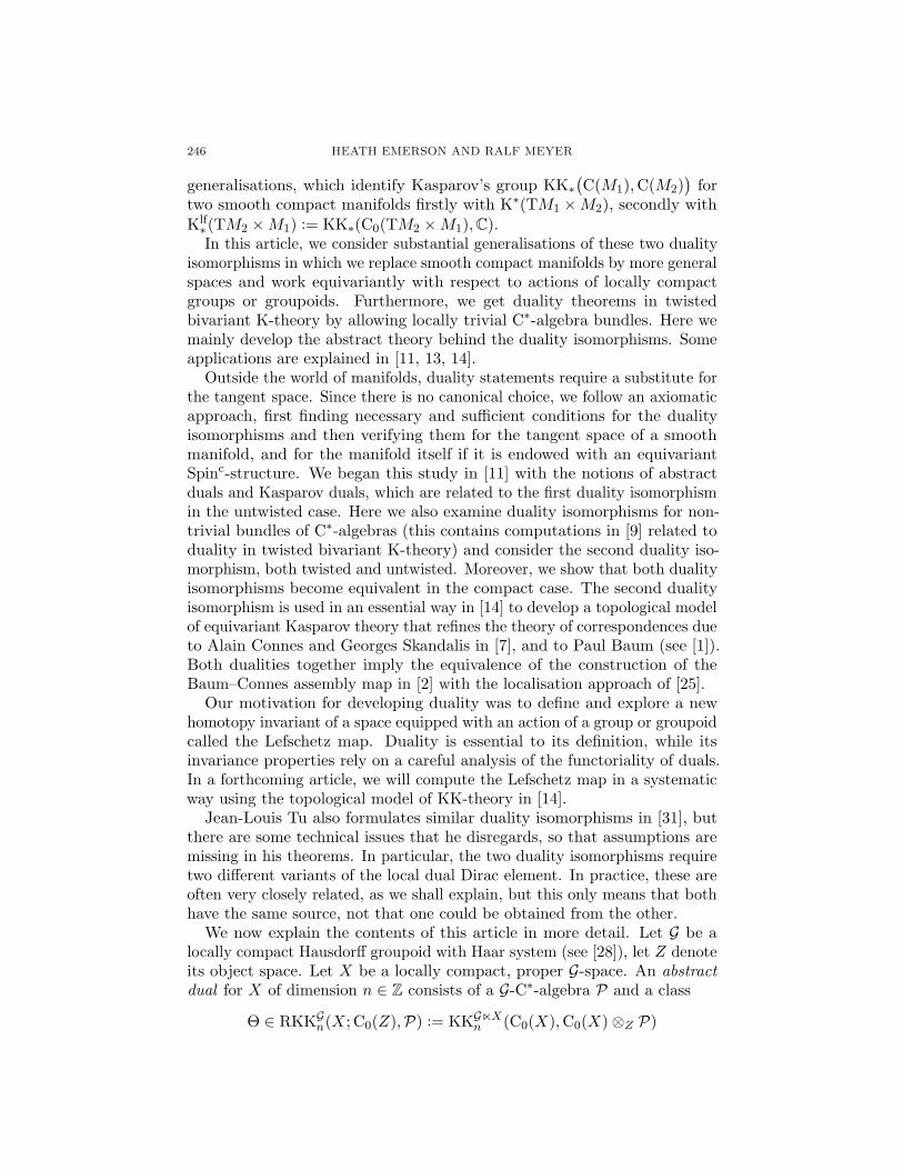
246 HEATH EMERSON AND RALF MEYER

generalisations, which identify Kasparov’s group KK∗(C(M1),C(M2)

)for

two smooth compact manifolds firstly with K∗(TM1 ×M2), secondly withKlf∗(TM2 ×M1) := KK∗(C0(TM2 ×M1),C).In this article, we consider substantial generalisations of these two duality

isomorphisms in which we replace smooth compact manifolds by more generalspaces and work equivariantly with respect to actions of locally compactgroups or groupoids. Furthermore, we get duality theorems in twistedbivariant K-theory by allowing locally trivial C∗-algebra bundles. Here wemainly develop the abstract theory behind the duality isomorphisms. Someapplications are explained in [11, 13, 14].

Outside the world of manifolds, duality statements require a substitute forthe tangent space. Since there is no canonical choice, we follow an axiomaticapproach, first finding necessary and sufficient conditions for the dualityisomorphisms and then verifying them for the tangent space of a smoothmanifold, and for the manifold itself if it is endowed with an equivariantSpinc-structure. We began this study in [11] with the notions of abstractduals and Kasparov duals, which are related to the first duality isomorphismin the untwisted case. Here we also examine duality isomorphisms for non-trivial bundles of C∗-algebras (this contains computations in [9] related toduality in twisted bivariant K-theory) and consider the second duality iso-morphism, both twisted and untwisted. Moreover, we show that both dualityisomorphisms become equivalent in the compact case. The second dualityisomorphism is used in an essential way in [14] to develop a topological modelof equivariant Kasparov theory that refines the theory of correspondences dueto Alain Connes and Georges Skandalis in [7], and to Paul Baum (see [1]).Both dualities together imply the equivalence of the construction of theBaum–Connes assembly map in [2] with the localisation approach of [25].

Our motivation for developing duality was to define and explore a newhomotopy invariant of a space equipped with an action of a group or groupoidcalled the Lefschetz map. Duality is essential to its definition, while itsinvariance properties rely on a careful analysis of the functoriality of duals.In a forthcoming article, we will compute the Lefschetz map in a systematicway using the topological model of KK-theory in [14].

Jean-Louis Tu also formulates similar duality isomorphisms in [31], butthere are some technical issues that he disregards, so that assumptions aremissing in his theorems. In particular, the two duality isomorphisms requiretwo different variants of the local dual Dirac element. In practice, these areoften very closely related, as we shall explain, but this only means that bothhave the same source, not that one could be obtained from the other.

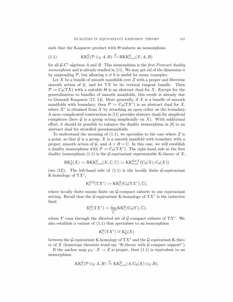
We now explain the contents of this article in more detail. Let G be alocally compact Hausdorff groupoid with Haar system (see [28]), let Z denoteits object space. Let X be a locally compact, proper G-space. An abstractdual for X of dimension n ∈ Z consists of a G-C∗-algebra P and a class

Θ ∈ RKKGn(X; C0(Z),P) := KKGnX

n (C0(X),C0(X)⊗Z P)

DUALITIES IN EQUIVARIANT KASPAROV THEORY 247

such that the Kasparov product with Θ induces an isomorphism

(1.1) KKG∗ (P ⊗Z A,B)

∼=−→ RKKG∗+n(X;A,B)

for all G-C∗-algebras A and B. This isomorphism is the first Poincare dualityisomorphism and is already studied in [11]. We may get rid of the dimension nby suspending P, but allowing n 6= 0 is useful for many examples.

Let X be a bundle of smooth manifolds over Z with a proper and fibrewisesmooth action of G, and let TX be its vertical tangent bundle. ThenP := C0(TX) with a suitable Θ is an abstract dual for X. Except for thegeneralisation to bundles of smooth manifolds, this result is already dueto Gennadi Kasparov [17, §4]. More generally, if X is a bundle of smoothmanifolds with boundary, then P := C0(TX◦) is an abstract dual for X,where X◦ is obtained from X by attaching an open collar on the boundary.A more complicated construction in [11] provides abstract duals for simplicialcomplexes (here G is a group acting simplicially on X). With additionaleffort, it should be possible to enhance the duality isomorphism in [8] to anabstract dual for stratified pseudomanifolds.

To understand the meaning of (1.1), we specialise to the case where Z isa point, so that G is a group, X is a smooth manifold with boundary with aproper, smooth action of G, and A = B = C. In this case, we will establisha duality isomorphism with P := C0(TX◦). The right-hand side in the firstduality isomorphism (1.1) is the G-equivariant representable K-theory of X,

RK∗G(X) := RKKG

∗+n(X; C,C) := KKGnX∗+n

(C0(X),C0(X)

)(see [12]). The left-hand side of (1.1) is the locally finite G-equivariantK-homology of TX◦,

KG,lf∗ (TX◦) := KKG

∗ (C0(TX◦),C),

where locally finite means finite on G-compact subsets in our equivariantsetting. Recall that the G-equivariant K-homology of TX◦ is the inductivelimit

KG∗ (TX◦) := lim−→

Y

KKG∗ (C0(Y ),C),

where Y runs through the directed set of G-compact subsets of TX◦. Wealso establish a variant of (1.1) that specialises to an isomorphism

KG∗ (TX◦) ∼= K∗

G(X)

between the G-equivariant K-homology of TX◦ and the G-equivariant K-theo-ry of X (homotopy theorists woud say “K-theory with G-compact support”).

If the anchor map pX : X → Z is proper, then (1.1) is equivalent to anisomorphism

KKG∗ (P ⊗Z A,B)

∼=−→ KKG∗+n(A,C0(X)⊗Z B),


that is, to a duality between C0(X) and P in the tensor category KKG (seeSection 5). But in general, abstract duals cannot be defined purely insideKKG .

Abstract duals are unique up to KKG-equivalence and covariantly functorialfor continuous, not-necessarily-proper G-equivariant maps: if P and P ′ areabstract duals for two G-spaces X and X ′, then a continuous G-equivariantmap f : X → X ′ induces a class αf ∈ KKG

∗ (P,P ′), and f 7→ αf is functorialin a suitable sense.

For instance, if X is a universal proper G-space and X ′ = Z, then thecanonical projection X → Z induces a class αf ∈ KKG

0

(P,C0(Z)

). This

plays the role of the Dirac morphism of [25] — in the group case, it is theDirac morphism — which is an important ingredient in the description ofthe Baum–Connes assembly map via localisation of categories. This exampleshows that abstract duals allow us to translate constructions from homotopytheory to noncommutative topology.

In contrast, C0(X) is contravariantly functorial, and only for proper maps.Thus the map from the classifying space to a point does not induce anythingon C0(X).

An abstract dual for a G-space X gives rise to a certain grading preservinggroup homomorphism

(1.2) Lef : RKKG∗(X; C0(X),C0(Z)

)→ KKG

∗(C0(X),C0(Z)

).

This is the Lefschetz map alluded to above. The functoriality of duals impliesthat it only depends on the proper G-homotopy type of X. There is a naturalmap

KKG∗(C0(X),C0(X)

)→ RKKG

∗(X; C0(X),C0(Z)

)which sends the class of a G-equivariant proper map ϕ : X → X to its graph

ϕ : X → X ×Z X, ϕ(x) := (x, ϕ(x)).

Since the latter map is proper even if the original map is not, we can think ofthe domain of Lef as not-necessarily-proper KK-self-maps of X. Combiningboth maps, we thus get a map

Lef : KKG∗(C0(X),C0(X)

)→ KKG

∗ (C0(X),C(Z)).

The Euler characteristic of X already defined in [11] is the equivariantLefschetz invariant of the identity map on X. With the specified domain (1.2),the map Lef is split surjective, so that Lefschetz invariants can be arbitrarilycomplicated. Usually, the Lefschetz invariants of ordinary self-maps are quitespecial and can be represented by ∗-homomorphisms to the C∗-algebra ofcompact operators on some graded G-Hilbert space (see [13]).

In many examples of abstract duals, the G-C∗-algebra P has the additionalstructure of a GnX-C∗-algebra. In this case, we arrive at explicit conditionsfor (1.1) to be an isomorphism, which also involve explicit formulas for the


inverse of the duality isomorphism (1.1) and for the Lefschetz map (seeTheorem 4.6 and Equation (4.27)). These involve the tensor product functor

TP : RKKG∗ (X;A,B) → KKG

∗ (P ⊗Z A,P ⊗Z B)

and a class D ∈ KKG−n

(P,C0(Z)

)which is determined uniquely by Θ. Since

the conditions for the duality isomorphism (1.1) are already formulatedimplicitly in [17, §4], we call this situation Kasparov duality.

The formula for the inverse isomorphism to (1.1) makes sense in greatergenerality: for any G nX-C∗-algebra A, we get a canonical map

(1.3) KKGnX∗ (A,C0(X)⊗Z B) → KKG

∗ (A⊗X P, B).

This is a more general situation because A is allowed to be a nontrivialbundle over X. If A is a trivial bundle C0(X,A0), then A⊗X P ∼= A0 ⊗ Pand the isomorphism in (1.3) is the inverse map to (1.1). It is shown in [9]that the map (1.3) is an isomorphism in some cases, but not always; thisdepends on whether or not the bundle A is locally trivial in a sufficientlystrong (equivariant) sense. Theorem 4.42 provides a necessary and sufficientcondition for (1.3) to be an isomorphism.

We verify these conditions for the tangent duality if X is a bundle ofsmooth manifolds with boundary and the bundle A is strongly locally trivial.Let A be a continuous trace algebra with spectrum X and a sufficiently niceG-action, so that duality applies, and let B = C0(Z) in (1.3). Let A∗ be theinverse of A in the G-equivariant Brauer group of X, that is, A ⊗X A∗ isG-equivariantly Morita equivalent to C0(X). Now the left-hand side in (1.3)may be interpreted as the G-equivariant twisted representable K-theory of Xwith twist A∗ because tensoring with A∗ provides an isomorphism

KKGnX∗

(A,C0(X)

) ∼= KKGnX∗ (C0(X), A∗).

But the right-hand side of (1.3) is KKG∗(A⊗X C0(TX◦),C0(Z)

), that is, the

locally finite G-equivariant twisted K-homology of TX◦, where the twist isgiven by the pull-back of A.

Thus (1.3) contains a twisted and groupoid-equivariant version of thefamiliar isomorphism K∗(X) ∼= Klf

∗(TX) for smooth compact manifolds (seealso [32]).

In addition, we get a canonical map

lim−→KKGnX∗ (A|Y ,C0(X)⊗Z B) → lim−→KKG

∗ (A|Y ⊗X P, B),

where Y runs through the directed set of G-compact subsets of X. If X is abundle of smooth manifolds with boundary, A is strongly locally trivial, and Pis C0(TX◦), then the latter map is an isomorphism as well. This specialisesto an isomorphism KG

∗ (TX◦) ∼= K∗G(X) for A = C0(X) and B = C0(Z).

We now discuss the second duality isomorphism, which generalises theisomorphism K∗(X) ∼= K∗(TX) for smooth compact manifolds. Kasparovonly formulates it for compact manifolds with boundary (see [17, Theorem


4.10]), and it is not obvious how best to remove the compactness assumption.We propose to consider the canonical map

(1.4) KKGnX∗+n (A,B ⊗Z P) → KKG

∗ (A,B),

that first forgets the X-structure and then composes with

D ∈ KKG−n

(P,C0(Z)

).

Here A is a G n X-C∗-algebra and B is a G-C∗-algebra. For instance, ifA = C0(X) and B = C0(Z), then this becomes a map

KKGnX∗+n (C0(X),P) → KKG

∗(C0(X),C0(Z)

),

that is, the right-hand side is the G-equivariant locally finite K-homology ofX.For the tangent duality P = C0(TX◦), the left-hand side is, by definition,the G-equivariant K-theory of TX◦ with X-compact support (see [12]).

Theorem 6.4 provides a necessary and sufficient condition for (1.4) tobe an isomorphism. It is shown in Section 7 that these conditions holdfor the tangent dual of a bundle X of smooth manifolds with boundary.Hence (1.4) specialises to an isomorphism KG,lf

∗ (X) ∼= RK∗G,X(TX◦) between

the G-equivariant locally finite K-homology of X and the G-equivariantK-theory of TX◦ with X-compact support.

As in the first duality isomorphism, we get a version of the second dualityisomorphism in twisted equivariant K-theory if we allow A to be a stronglylocally trivial G-equivariant bundle of C∗-algebras over X: the twistedG-equivariant locally finite K-homology of X with twist A is isomorphic tothe twisted G-equivariant K-theory of TX◦ with X-compact support andwith twist A∗. And we get a version with different support conditions:

(1.5) lim−→KKGnX∗+n (A|Y , B ⊗Z P) → lim−→KKG

∗ (A|Y , B),

where Y runs through the directed set of G-compact subsets of X. Forbundles of smooth manifolds, the latter specialises to an isomorphism

K∗G(TX◦) ∼= KG

∗ (X).

The duality isomorphism (1.4) for the tangent space dual specialises to anisomorphism

(1.6) RKG∗,X(Y ×Z TX◦) ∼= KKG

∗(C0(X),C0(Y )

).

The first group is the home for symbols of families of elliptic pseudodifferentialoperators on X parametrised by Y . There are different formulas for thisisomorphism, using a topological index map or the family of Dolbeaultoperators along the fibres of TX◦ → Z, or pseudodifferential calculus. Theseare based on different formulas for the class D involved in the dualityisomorphisms. Since D is determined uniquely by Θ, for which there isonly one reasonable geometric formula, duality isomorphisms also containequivariant index theorems such as Kasparov’s Index Theorem [15].

The duality isomorphism (1.6) is the crucial step in the geometric descrip-tion of Kasparov theory in [14]. The question when this can be done remained


unexamined since Paul Baum introduced his bicycles or correspondencessome thirty years ago. Even for the special case of KK∗(C0(X),C) for afinite CW-complex X, a detailed proof appeared only recently in [3]. In [14],we prove that the equivariant Kasparov groups KKG

∗(C0(X),C0(Y )

)can be

described in purely topological terms if X is a bundle over Z of smoothmanifolds with boundary with a smooth action of a proper groupoid G andsome conditions regarding equivariant vector bundles are met.

The basic idea of the argument is that an isomorphism similar to (1.6)exists in the geometric theory. Thus the problem of identifying geomet-ric and analytic bivariant K-theory reduces to the problem of identifyingcorresponding monovariant K-theory groups with some support conditions.This becomes trivial with an appropriate definition of the geometric cycles.Besides finding this appropriate definition, the main work in [14] is necessaryto equip the geometric version of KK with all the extra structure that isneeded to get duality isomorphisms. Our analysis here already shows whatis involved: composition and exterior products and certain pull-back andforgetful functors.

Let X be a proper G-space and let B be a G nX-C∗-algebra. Then [12,Theorem 4.2] implies a natural isomorphism

(1.7) lim−→KKGnX∗ (C0(Y ), B) ∼= K∗(G nB),

where the inductive limit runs over the directed set of G-compact subsetsof X as in (1.5). Equations (1.4) and (1.7) yield a duality isomorphism

(1.8) lim−→KKG∗ (C0(Y ), B) ∼= K∗+n

(G n (P ⊗Z B)

).

If X is also a universal proper G-space, then our duality isomorphisms areclosely related to the different approaches to the Baum–Connes assembly mapfor G. The dual Dirac method is the main ingredient in most proofs of theBaum–Connes and Novikov Conjectures; this goes back to Gennadi Kasparov[17, 18], who used the first Poincare duality isomorphism to prove the NovikovConjecture for discrete subgroups of almost connected groups. We will seethat the first duality isomorphism for a groupoid G acting on its classifyingspace is essentially equivalent to constructing a Dirac morphism for thegroupoid, which is the (easier) half of the dual Dirac method. The remaininghalf, the dual Dirac morphism, is a lifting of Θ ∈ RKKGnX

∗(C0(X),C0(X)

)to KKG

∗(C0(Z),C0(Z)

). Even if such a lifting does not exist, the Dirac

morphism D ∈ KKG−n

(P,C0(Z)

)is exactly what is needed for the localisation

approach to the Baum–Connes assembly map in [25].The isomorphism (1.8) relates two approaches to the Baum–Connes as-

sembly map with coefficients. The left-hand side is the topological K-theorydefined in [2], whereas the right-hand side is the topological K-theory inthe localisation approach of [25]. This is exactly the γ-part of K∗(G n B)provided G has a γ-element.


Finally, we describe the contents of the following sections. Sections 2and 3 contain preparatory remarks on groupoids, their actions on spaces andC∗-algebras, and equivariant Kasparov theory for groupoids. We pay specialattention to tensor product functors because these will play a crucial role.

Section 4 deals with the first Poincare duality isomorphism and relatedconstructions. We introduce abstract duals and Kasparov duals and constructequivariant Euler characteristics and Lefschetz maps from them. We explainhow the first duality is related to Dirac morphisms and thus to the Baum–Connes assembly map, and we provide a necessary and sufficient conditionfor the first duality isomorphism to extend to nontrivial bundles, formalisingan example considered in [9].

Section 5 studies Kasparov duality for bundles of compact spaces. Inthis case, the first and second kind of duality are both equivalent to a morefamiliar notion of duality studied already by Georges Skandalis in [30].

Section 6 treats the second duality isomorphism. We introduce symmetricKasparov duals, which guarantee both duality isomorphisms for trivialbundles.

In Section 7, we construct symmetric Kasparov duals for bundles of smoothmanifolds with boundary. For a single smooth manifold, this example isalready considered in [17]. We also extend the duality isomorphisms tocertain locally trivial C∗-algebra bundles as coefficients.

1.1. Some standing assumptions. To avoid technical problems, we tac-itly assume all C∗-algebras to be separable, and all topological spaces to belocally compact, Hausdorff, and second countable. Groupoids are tacitlyrequired to be locally compact, Hausdorff, and second countable and to havea Haar system.

Several constructions of Kasparov duals contain Clifford algebras and henceyield Z/2-graded C∗-algebras. Therefore, we tacitly allow all C∗-algebra tocarry a Z/2-grading; that is, “C∗-algebra” stands for “Z/2-graded C∗-algebra”throughout.

The general theory in Sections 2–6 is literally the same for complex, real,and “real” C∗-algebras (although we usually presume in our notation thatwe are in the complex case). The construction of duals for bundles of smoothmanifolds in Section 7 also works for these three flavours, with some smallmodifications that are pointed out where relevant. Most importantly, theresults about tangent space duality claimed above only hold if the tangentbundle is equipped with a “real” structure or replaced by another vectorbundle.

2. Preliminaries on groupoid actions

We recall some basic notions regarding groupoids and their actions onspaces and C∗-algebras to fix our notation. We pay special attention totensor product operations and their formal properties, which are expressed


in the language of symmetric monoidal categories (see [23, 29, 27]). Thisframework is particularly suited to the first Poincare duality isomorphism.

2.1. Groupoids and their actions on spaces. Let G be a (locally com-pact) groupoid. We write G(0) and G(1) for the spaces of objects and mor-phisms in G and r, s : G(1) ⇒ G(0) for the range and source maps.

Definition 2.1. Let Z be a (locally compact, Hausdorff, second countabletopological) space. A space over Z is a continuous map f : X → Z. If f isclear from the context, we also call X itself a space over Z.

Definition 2.2. Let f : X → Z and g : Y → Z be spaces over Z. Theirfibred product is

X ×f,g Y := {(x, y) ∈ X × Y | f(x) = g(y)}

with the subspace topology and the continuous map (x, y) 7→ f(x) = g(y).Thus X ×f,g Y is again a space over Z. If f, g are clear from the context, wealso write X ×Z Y instead of X ×f,g Y .

Definition 2.3. A G-space is a space (X,π) over G(0) with the action givenby a map over G(0):

G(1) ×s,π X(g,x) 7→g·x //

p%%KKKKKKKKKK

X

π~~}}

}}}}

}}

G(0).

Here, the reference map p takes (g, x) to r(g), and the usual associativityand unitality diagrams commute. Note that we obtain a homeomorphism

G(1) ×s,π X → G(1) ×r,π X, (g, x) 7→ (g, g · x).

Example 2.4. If G is a group then G := G is a groupoid with G(0) = {?},and G-spaces have the usual meaning.

Example 2.5. View a space Z as a groupoid with only identity morphisms,that is, Z(1) = Z(0) = Z. A Z-space is nothing but a space over Z.

Definition 2.6. If Z is a G-space, then the transformation groupoid G n Zis the groupoid with (G n Z)(0) := Z,

(G n Z)(1) := G(1) ×s,π Z ∼= {(z1, g, z2) ∈ Z ×π,r G(1) ×s,π Z | z1 = g · z2},r(z1, g, z2) := z1, s(z1, g, z2) := z2, (z1, g, z2) · (z2, h, z3) := (z1, g · h, z3).

This groupoid inherits a Haar system from G.

Lemma 2.7. A GnZ-space is the same as a G-space X with a G-equivariantcontinuous map p : X → Z.


Hence we call GnZ-spaces G-spaces over Z. We are going to study dualityin bivariant K-theory for a G-space p : X → Z over Z or, equivalently, fora G n Z-space. Since we lose nothing by replacing G by G n Z, we mayassume from now on that Z = G(0) to simplify our notation. Thus, when westudy duality for bundles of spaces over some base space Z then this bundlestructure is hidden in the groupoid variable G.

2.2. C∗-algebras over a space. Let Z be a space. There are severalequivalent ways to define C∗-algebras over Z.

Definition 2.8. A C∗-algebra over Z is a C∗-algebra A together with anessential ∗-homomorphism ϕ from C0(Z) to the centre of the multiplieralgebra of A; being essential means that ϕ

(C0(Z)

)·A = A; equivalently, ϕ

extends to a strictly continuous unital ∗-homomorphism on Cb(Z).

The map ϕ is equivalent to a continuous map from the primitive ideal spaceof A to Z by the Dauns–Hofmann Theorem (see [26]). Any C∗-algebra over Zis the C∗-algebra of C0-sections of an upper semi-continuous C∗-bundle over Zby [26], and conversely such section algebras are C∗-algebras over Z. We mayalso describe a C∗-algebra over Z by the A-linear essential ∗-homomorphism

(2.9) m : C0(Z,A) → A, f ⊗ a 7→ ϕ(f) · a = a · ϕ(f),

called multiplication homomorphism. This ∗-homomorphism exists becauseC0(Z,A) is the maximal C∗-tensor product of C0(Z) and A, and it deter-mines ϕ.

Example 2.10. If p : X → Z is a space over Z, then C0(X) with

p∗ : C0(Z) → Cb(X)

is a commutative C∗-algebra over Z. Any commutative C∗-algebra over Z isof this form. The multiplication homomorphism

m : C0

(Z,C0(X)

) ∼= C0(Z ×X) → C0(X)

is induced by the proper continuous map X → Z ×X, x 7→(p(x), x

).

Definition 2.11. Let A and B be C∗-algebras over Z with multiplica-tion homomorphisms mA : C0(Z,A) → A and mB : C0(Z,B) → B. A∗-homomorphism f : A → B is called C0(Z)-linear or Z-equivariant if thefollowing diagram commutes:

C0(Z,A)C0(Z,f) //

mA

��

C0(Z,B)

mB

��A

f // B.

Definition 2.12. We let C∗Z be the category whose objects are the C∗-alge-bras over Z and whose morphisms are the C0(Z)-linear ∗-homomorphisms.


Definition 2.13. Let A be a C∗-algebras over Z and let S ⊆ Z be a subset.If S is closed or open, then we define a restriction functor |S : C∗Z → C∗S :

• If S is open, then A|S is the closed ∗-ideal C0(S) ·A in A, equippedwith the obvious structure of C∗-algebra over S.

• If S is closed, then A|S is the quotient of A by the ideal A|Z\S ,equipped with the induced structure of C∗-algebra over S.

We abbreviate Az := A|{z} for z ∈ Z.

If S1 ⊆ S2 ⊆ Z are both closed or both open in Z, then we have a naturalisomorphism (A|S2)|S1

∼= A|S1 .

Definition 2.14. Let f : Z ′ → Z be a continuous map. Then we define abase change functor f∗ : C∗Z → C∗Z′ . Let A be a C∗-algebra over Z. ThenC0(Z ′, A) is a C∗-algebra over Z ′×Z. The graph of f is a closed subset Γ(f)of Z ′ × Z and homeomorphic to Z ′ via z 7→

(z, f(z)

). We let f∗(A) be the

restriction of C0(Z ′, A) to Γ(f), viewed as a C∗-algebra over Z ′. It is clearthat this construction is natural, that is, defines a functor f∗ : C∗Z → C∗Z′ .

Lemma 2.15. Let f : Z ′ → Z be a continuous map, let A be a C∗-algebraover Z and let B be a C∗-algebra. Then essential ∗-homomorphisms f∗(A) →M(B) correspond bijectively to pairs of commuting essential ∗-homomor-phisms π : A→M(B) and ϕ : C0(Z ′) →M(B) that satisfy ϕ(h ◦ f) · π(a) =π(h · a) for all h ∈ C0(Z), a ∈ A.

This universal property characterises the base change functor uniquely upto natural isomorphism and implies the following properties:

Lemma 2.16. If f : S → Z is the embedding of an open or closed subset,then f∗(A) is naturally isomorphic to A|S.

We have (g ◦ f)∗ = g∗ ◦ f∗ for composable maps Z ′′f−→ Z ′

g−→ Z, and id∗Zis equivalent to the identity functor. In particular, f∗(A)z

∼= Af(z).

Notation 2.17. Let A and B be C∗-algebras over Z. Then A ⊗ B is aC∗-algebra over Z × Z. We let A⊗Z B be its restriction to the diagonal inZ × Z.

Example 2.18. Let (X, p) be a space over Z. If S ⊆ Z, then restrictionyields C0(X)|S = C0

(p−1(S)

)as a space over S.

Now let f : Z ′ → Z be a continuous map. Then

f∗(C0(X)

) ∼= C0(X ×p,f Z′).

In particular, f∗(C0(Z)

) ∼= C0(Z ′).We have C0(X1)⊗Z C0(X2) ∼= C0(X1×Z X2) if X1 and X2 are two spaces

over Z.

The properties of the tensor product ⊗Z are summarised in Lemma 2.22below. For the time being, we note that it is a bifunctor and that it is


compatible with the functors f∗: if f : Z ′ → Z is a continuous map, thenthere is a natural isomorphism

f∗(A⊗Z B) ∼= f∗(A)⊗Z′ f∗(B)

because both sides are naturally isomorphic to restrictions of C0(Z ′ × Z ′)⊗A⊗B to the same copy of Z ′ in Z ′ × Z ′ × Z × Z.

2.3. Groupoid actions on C∗-algebras and tensor products. Let Gbe a groupoid with object space Z := G(0).

Definition 2.19. LetA be a C∗-algebra over Z together with an isomorphismα : s∗(A)

∼=−→ r∗(A) of C∗-algebras over G(1). Let Az for z ∈ Z denote thefibres of A and let αg : As(g)

∼=−→ Ar(g) for g ∈ G(1) be the fibres of α. We call(A,α) a G-C∗-algebra if αg1g2 = αg1αg2 for all g1, g2 ∈ G(1).

Definition 2.20. A ∗-homomorphism ϕ : A→ B between two G-C∗-algebrasis called G-equivariant if it is C0(Z)-linear and the diagram

s∗(A)

∼=α

��

s∗(ϕ) // s∗(B)

∼=β��

r∗(A)r∗(ϕ) // r∗(B)

commutes. We let C∗G be the category whose objects are the G-C∗-algebrasand whose morphisms are the G-equivariant ∗-homomorphisms.

This agrees with our previous definitions if G is a space viewed as agroupoid with only identity morphisms.

The tensor product over Z of two G-C∗-algebras carries a canonical ac-tion of G called diagonal action. Formally, this is the composite of the∗-isomorphisms

s∗(A⊗G(0)B)∼=−→ s∗(A)⊗G(1)s∗(B)

α⊗G(1)β−−−−−→r∗(A)⊗G(1)r∗(B)

∼=−→ r∗(A⊗G(0)B).

Notation 2.21. The resulting tensor product operation on G-C∗-algebrasis denoted by ⊗G . We usually abbreviate ⊗G to ⊗ and also write ⊗Z .

Lemma 2.22. The category C∗G with the tensor product ⊗ is a symmetricmonoidal category with unit object C0(Z).

A symmetric monoidal category is a category with a tensor productfunctor ⊗, a unit object 1, and natural isomorphisms

(A⊗B)⊗ C ∼= A⊗ (B ⊗ C), A⊗B ∼= B ⊗A, 1⊗A ∼= A ∼= A⊗ 1

called associativity, commutativity, and unitality constraints; these are sub-ject to various coherence laws, for which we refer to [29]. These condi-tions allow to define tensor products

⊗x∈F Ax for any finite set of ob-

jects (Ax)x∈F with the expected properties such as natural isomorphisms

DUALITIES IN EQUIVARIANT KASPAROV THEORY 257⊗x∈F1

Ax ⊗⊗

x∈F2Ax

∼=⊗

x∈F Ax for any decomposition F = F1 t F2 intodisjoint subsets. The associativity, commutativity, and unitality constraintsare obvious in our case, and the coherence laws are trivial to verify. Therefore,we omit the details.

Let G1 and G2 be groupoids and let f : G1 → G2 be a continuous functor.Let f (0) and f (1) be its actions on objects and morphisms, respectively. If Ais a G2-C∗-algebra with action α, then (f (0))∗(A) is a G1-C∗-algebra for theaction

s∗1(f(0))∗(A) ∼= (f (0)s1)∗(A) = (s2f (1))∗(A) ∼= (f (1))∗s∗2(A)

(f (1))∗(α)−−−−−−→ (f (1))∗r∗2(A) ∼= (r2f (1))∗(A) = (f (0)r1)∗(A) ∼= r∗1(f(0))∗(A).

This defines a functorf∗ : C∗G2

→ C∗G1,

which is symmetric monoidal, that is, we have canonical isomorphisms

(2.23) f∗(A)⊗G1 f∗(B) ∼= f∗(A⊗G2 B)

that are compatible in a suitable sense with the associativity, commutativity,and unitality constraints in C∗G2

and C∗G1(we refer to [29] for the precise

definition). The natural transformation in (2.23) is part of the data of asymmetric monoidal functor. Again we omit the proof because it is trivialonce it is clear what has to be checked. As a consequence, f∗ preserves tensorunits, that is,

f∗(C0(G(0)

2 )) ∼= C0(G(0)

1 ).Let X be a G-space. Then the category C∗GnX carries its own tensor

product, which we always denote by ⊗X , to distinguish it from the tensorproduct ⊗ in C∗G . The projection map pX : G nX → G induces a functor

p∗X : C∗G → C∗GnX ,

which acts by A 7→ C0(X)⊗Z A on objects. We have seen above that suchfunctors are symmetric monoidal, that is, if A and B are G-C∗-algebras, then

(2.24) p∗X(A)⊗X p∗X(B) ∼= p∗X(A⊗B).

If A is a G nX-C∗-algebra and B is merely a G-C∗-algebra, then A⊗Z Bis a G nX-C∗-algebra. This defines another tensor product operation

⊗ = ⊗Z : C∗GnX × C∗G → C∗GnX ,

which has obvious associativity and unitality constraints

(A⊗B)⊗ C ∼= A⊗ (B ⊗ C), A⊗ 1 ∼= A,

where A belongs to C∗GnX , B and C belong to C∗G , and 1 is the unit object,here C0(Z). These natural isomorphisms satisfy the relevant coherence lawsformalised in [27]. In the notation of [27], C∗GnX is a C∗G-category.

Our two tensor products are related by a canonical isomorphism

(2.25) A⊗B ∼= A⊗X p∗X(B),


or, more precisely,

A⊗X p∗X(B) := A⊗X (C0(X)⊗B) ∼=(A⊗X C0(X)

)⊗B ∼= A⊗B.

These isomorphisms are all natural and G nX-equivariant.We also have a canonical forgetful functor

forgetX : C∗GnX → C∗G ,

which maps a G-C∗-algebra over X to the underlying G-C∗-algebra, forgettingthe X-structure. This is a C∗G-functor in the notation of [27], that is, thereare natural isomorphisms

forgetX(A⊗B) ∼= forgetX(A)⊗B

for A in C∗GnX and B in C∗G , and these isomorphisms are compatible withthe associativity and unitality constraints.

3. Equivariant Kasparov theory for groupoids

We use the equivariant Kasparov theory for C∗-algebras with groupoidactions by Pierre-Yves Le Gall [22]. Let G be a groupoid with objectspace Z. Le Gall defines Z/2-graded Abelian groups KKG

∗ (A,B) for (possiblyZ/2-graded) G-C∗-algebras A and B. He also constructs a Kasparov cup-capproduct

(3.1) ⊗D : KKG∗ (A1, B1⊗D)×KKG

∗ (D⊗A2, B2) → KKG∗ (A1⊗A2, B1⊗B2)

in KKG with the expected properties such as associativity in general andgraded commutativity of the exterior product (see [22, §6.3]). Throughoutthis section, ⊗ denotes the tensor product over Z, so that it would be moreprecise to write ⊗Z,D instead of ⊗D.

Notation 3.2. When we write KKG∗ (A,B), we always mean the Z/2-graded

group. We write KKG0 (A,B) and KKG

1 (A,B) for the even and odd parts ofKKG

∗ (A,B). We let KKG be the category whose objects are the (separable,Z/2-graded) G-C∗-algebras and whose morphism spaces are KKG

∗ (A,B), withcomposition given by the Kasparov composition product.

Example 3.3. If G is a locally compact group, viewed as a groupoid, thenLe Gall’s bivariant K-theory agrees with Kasparov’s theory defined in [17].

Example 3.4. If G = GnX for a locally compact group G and a locally com-pact G-space X, then KKG

∗ (A,B) agrees with Kasparov’s RKKG∗ (X;A,B).

This also contains Kasparov’s groups RKKG∗ (X;A,B) for two G-C∗-algebras

A and B as a special case because

RKKG∗ (X;A,B) := RKKG

∗(X; C0(X,A),C0(X,B)

).

The cup-cap product (3.1) contains an exterior tensor product operation

⊗ = ⊗Z : KKG × KKG → KKG , (A,B) 7→ A⊗B,


which extends the tensor product on C∗G and turns KKG into an additivesymmetric monoidal category (see [29, 24]). That is, the associativity, com-mutativity, and unitality constraints that exist in C∗G descend to naturaltransformations on KKG ; this follows from the universal property of KKG inthe ungraded case or by direct inspection. Fixing one variable, we get theexterior product functors

σD : KKG → KKG , A 7→ A⊗D,

for all G-C∗-algebras D. These are additive KKG-functors, that is, there arenatural isomorphisms σD(A⊗B) ∼= σD(A)⊗B with good formal properties(see [27]).

If G1 and G2 are two groupoids and f : G1 → G2 is a continuous functor,then the induced functor f∗ : C∗G2

→ C∗G1descends to an additive functor

f∗ : KKG2 → KKG1 ,

that is, there are canonical maps

(3.5) f∗ : KKG2∗ (A,B) → KKG1

∗(f∗(A), f∗(B)

)for all G2-C∗-algebras A and B. These maps are compatible with the cup-capproduct in (3.1), so that f∗ is a symmetric monoidal functor. More precisely,the natural isomorphisms f∗(A) ⊗G1 f

∗(B) ∼= f∗(A ⊗G2 B) in C∗G1remain

natural when we enlarge our morphism spaces from ∗-homomorphisms toKK.

Le Gall describes in [22] how to extend this functoriality to Hilsum–Skandalis morphisms between groupoids. As a consequence, KKG1 and KKG2

are equivalent as symmetric monoidal categories if the groupoids G1 and G2

are equivalent.We are mainly interested in the special case of (3.5) where we consider

the functor G nX → G n Z = G induced by the projection pX : X → Z fora G-space X. This yields an additive, symmetric monoidal functor

(3.6) p∗X : KKG → KKGnX ,

which acts on objects by A 7→ C0(X)⊗A.The canonical tensor products in the categories KKGnX and KKG are over

Z and X, respectively. Therefore, we denote the tensor product in KKGnX

by ⊗X .The tensor product operation

⊗ = ⊗Z : C∗GnX × C∗G → C∗GnX

also descends to the Kasparov categories, yielding a bifunctor

(3.7) ⊗ = ⊗Z : KKGnX × KKG → KKGnX

that is additive in each variable. The easiest construction uses (2.25). The bi-functor so defined obviously satisfies the associativity and unitality conditionsneeded for a KKG-category (see [27]).


The forgetful functor descends to an additive functor

forgetX : KKGnX → KKG

between the Kasparov categories. This is a KKG-functor in the notationof [27]. The obvious C∗-algebra isomorphisms

forgetX(A⊗B) ∼= forgetX(A)⊗B

for all G nX-C∗-algebras A and all G-C∗-algebras B remain natural on thelevel of Kasparov categories.

Since many constructions do not work for arbitrary G nX-C∗-algebras,we often restrict to the following full subcategory of KKGnX :

Definition 3.8. Let A and B be G-C∗-algebras. We define

RKKG∗ (X;A,B) := KKGnX

∗(p∗X(A), p∗X(B)

),

and we let RKKG(X) be the category whose objects are the G-C∗-algebrasand whose morphism spaces are RKKG

0 (X;A,B). By definition, RKKG isthe (co)image of the functor p∗X in (3.6). We often view RKKG(X) as a fullsubcategory of KKGnX .

Example 3.9. Let G be a group G, so that Z = ?. Then X is just a G-space,and KKG = KKG is the usual group-equivariant Kasparov category. We havep∗X(A) = C0(X,A) in this case, so that p∗X : KKG → RKKG(X) is the samefunctor as in [11, Equation (7)]. The functor forgetX : RKKG(X) → KKG

agrees with the forgetful functor in [11, Equation (6)].

The subcategory RKKG(X) ⊆ KKGnX is closed under the tensor productoperations ⊗X and ⊗Z . Hence it is a symmetric monoidal category and aKKG-category in its own right.

A G-equivariant map f : X1 → X2 induces a functor f∗ : KKGnX2 →KKGnX1 , which restricts to a functor

f∗ : RKKG(X2) → RKKG(X1).

This functoriality contains grading preserving group homomorphisms

f∗ : RKKG∗ (X2;A,B) → RKKG

∗ (X1;A,B),

which are compatible with cup-cap products in both variables A and B.These maps also turn X 7→ RKKG

∗ (X;A,B) into a functor from the categoryof locally compact G-spaces with G-equivariant continuous maps to thecategory of Z/2-graded Abelian groups. This is a homotopy functor, that is,two G-equivariantly homotopic maps induce the same map on RKKG

∗ (seeExample 5.3 below for a proof).

Notation 3.10. Let P be a G nX-C∗-algebra. Then there is an associatedfunctor

σP : KKGnX → KKGnX , A 7→ P ⊗X A.


We denote the composite functor

RKKG(X) ⊆−→ KKGnXσP−−→ KKGnX

forgetX−−−−→ KKG

by TP . We have TP(A) = P ⊗A for a G-C∗-algebra A, viewed as an objectof RKKG(X), because of the natural isomorphisms P ⊗X p∗X(A) ∼= P ⊗ A.Thus TP determines maps

TP : RKKG∗ (X;A,B) := KKGnX

∗(p∗X(A), p∗X(B)

)→ KKG

∗ (P ⊗A,P ⊗B).

The functor TP is the analogue for groupoids of the functor that is calledσX,P in [11]. If f ∈ KKG

∗ (A,B), then

(3.11) TP(p∗X(f)

)= σP(f) = idP ⊗ f in KKG

∗ (P ⊗A,P ⊗B).

This generalises [11, Equation (26)].

4. The first duality

Let G be a locally compact groupoid and let Z := G(0) with the canonical(left) G-action, so that G n Z ∼= G. Let X be a G-space. The notion of anequivariant Kasparov dual for group actions in [11] can be copied literally toour more general setup. To clarify the relationship, we write

1 := C0(Z), 1X := C0(X).

These are the tensor units in KKG and KKGnX , respectively. Wherever Cappears in [11], it is replaced by 1. Furthermore, we write TP instead of σX,Pand 1X instead of C0(X) here.

Definition 4.1. Let n ∈ Z. An n-dimensional G-equivariant Kasparov dualfor the G-space X is a triple (P, D,Θ), where

• P is a (possibly Z/2-graded) G nX-C∗-algebra,• D ∈ KKG

−n(P,1), and• Θ ∈ RKKG

n(X;1,P),subject to the following three conditions:

Θ⊗P D = id1 in RKKG0 (X;1,1);(4.2)

Θ⊗X f = Θ⊗P TP(f) in RKKG∗+n(X;A,P ⊗B)(4.3)

for all G-C∗-algebras A and B and all f ∈ RKKG∗ (X;A,B);

TP(Θ)⊗P⊗P flipP = (−1)nTP(Θ) in KKGn(P,P ⊗ P),(4.4)

where flipP is the flip automorphism on P ⊗ P as in [11].

This differs slightly from the definition of a Kasparov dual in [11, Definition18] because (4.3) contains no auxiliary space Y as in [11]. As a result,(P, D,Θ) is a Kasparov dual in the sense of [11] if and only if its pull-backto Z ′ is a Kasparov dual for Z ′ ×Z X, viewed as a G n Z ′-space, for anyG-space Z ′. The space Z ′ plays no significant role and is only added in [11]


because this general setting is considered in [17]. We expect that geometricsufficient conditions for Kasparov duals are invariant under this base changeoperation.

The notion of dual in Definition 4.1 is relative to the base space Z. In asense, a G-equivariant Kasparov dual is a G-equivariant family of Kasparovduals for the fibres of the map pX : X → Z.

We remark without proof that (4.4) is equivalent, in the presence of theother two conditions, to

(4.5) TP(Θ)⊗P⊗P (D ⊗ idP) = (−1)nidP in KKG0 (P,P)

(the easier implication (4.4)=⇒(4.5) is contained in Lemma 4.11). Bothformulations (4.4) and (4.5) tend to be equally hard to check.

Condition (4.3) is not so difficult to check in practice, but it lacks goodfunctoriality properties and is easily overlooked (such as in [31, Theoreme5.6]). This condition turns out to be automatic for universal proper G-spaces(Lemma 4.31). We will comment further on its role in Section 5, where wediscuss the special case where the map pX : X → Z is proper.

Theorem 4.6. Let P be a G nX-C∗-algebra, n ∈ Z, D ∈ KKG−n(P,1), and

Θ ∈ RKKGn(X;1,P). The natural transformations

PD: KKGi−n(P ⊗A,B) → RKKG

i (X;A,B), f 7→ Θ⊗P f,PD∗ : RKKG

i (X;A,B) → KKGi−n(P ⊗A,B), g 7→ (−1)inTP(g)⊗P D

are inverse to each other for all G-C∗-algebras A and B if and only if(P, D,Θ) is a G-equivariant Kasparov dual for X. In this case, the functorTP : RKKG(X) → KKG is left adjoint to the functor p∗X : KKG → RKKG(X).

We call the isomorphism in Theorem 4.6 Kasparov’s first duality isomor-phism because it goes back to Gennadi Kasparov’s proof of his First PoincareDuality Theorem [17, Theorem 4.9]. We postpone the proof of Theorem 4.6to Section 4.1.2 in order to utilise some more notation that we need also forother purposes.

Kasparov duals need not exist in general, even if the groupoid G is trivialand Z = ?. The Cantor set is a counterexample (see Proposition 5.9).

To construct a Kasparov dual for a space, we need some geometric infor-mation on the space in question. For instance, for a smooth manifold we caneither use Clifford algebras or the tangent bundle to construct a Kasparovdual. We may also triangulate the manifold and use this to construct a morecombinatorial dual.

We will use Kasparov duals to construct Lefschetz invariants and Eulercharacteristics. This leads to the question how unique Kasparov duals areand whether other notions derived from them may depend on choices. Thefollowing counterexample shows that Kasparov duals are not unique.

Example 4.7. Let G be the trivial groupoid, so that Z := ? is the one-point space, and let X := [0, 1]. The homotopy invariance of RKK in the


space-variable implies

RKK∗(X;A,B) ∼= RKK∗(?;A,B) = KK∗(A,B)

for all C∗-algebras A and B.Let P := C([0, 1]), let D be the class of an evaluation homomorphism,

and let Θ be the class of the map C([0, 1]) → C([0, 1] × [0, 1]), f 7→ f ⊗ 1.Inspection shows that this is a Kasparov dual for X. So is P ′ := C, viewedas a C∗-algebra over [0, 1] by evaluation at any point, with D′ and Θ′ beingthe identity maps. While P and P ′ are homotopy equivalent and henceisomorphic in KK, they are not isomorphic in RKK([0, 1]) because their fibresare not KK-equivalent everywhere.

Abstract duals formalise what is unique about Kasparov duals. This isimportant because constructions that can be expressed in terms of abstractduals yield equivalent results for all Kasparov duals. The equivalence betweenthe smooth and combinatorial duals for smooth manifolds is used in [11, 13]to reprove an index theorem for the equivariant Euler operator and theEquivariant Lefschetz Fixed Point Theorem of Wolfgang Luck and JonathanRosenberg (see [20, 21]).

Definition 4.8. Let P be a G-C∗-algebra and let Θ ∈ RKKGn(X;1,P).

We call the pair (P,Θ) an n-dimensional abstract dual for X if the mapPD defined as in Theorem 4.6 is an isomorphism for all G-C∗-algebras Aand B. We call (P,Θ) an n-dimensional weak abstract dual for X if PD isan isomorphism for A = 1X and all G-C∗-algebras B.

We can always adjust the dimension to be 0 by passing to a suspensionof P.

Theorem 4.6 shows that (P,Θ) is an abstract dual if (P, D,Θ) is a Kas-parov dual. We will see below that we can recover D and the functor TPfrom the abstract dual. The main difference between Kasparov duals andabstract duals is that for the latter, P is not necessarily a C∗-algebra over X.This is to be expected because of Example 4.7. We need weak abstractduals in connection with [14], for technical reasons, because computations inthe geometric version of KK may provide weak abstract duals, but not theexistence of a duality isomorphism for all G-C∗-algebras A.

Proposition 4.9. A weak abstract dual for a space X is unique up to acanonical KKG-equivalence if it exists, and even covariantly functorial in thefollowing sense.

Let X and Y be two G-spaces and let f : X → Y be a G-equivariantcontinuous map. Let (PX ,ΘX) and (PY ,ΘY ) be weak abstract duals forX and Y of dimensions nX and nY , respectively. Then there is a uniquePf ∈ KKG

nY −nX(PX ,PY ) with ΘX ⊗PX

Pf = f∗(ΘY ). Given two composablemaps between three spaces with duals, we have Pf◦g = Pf ◦ Pg. If X = Y ,f = idX , and (PX ,ΘX) = (PY ,ΘY ), then Pf = idPX

. If only X = Y ,f = idX , then Pf is a KKG-equivalence between the two duals of X.


Proof. The condition characterising Pf is equivalent to PDX(Pf ) = f∗(ΘY ),which uniquely determines Pf . The uniqueness of Pf implies identities suchas Pf◦g = Pf ◦ Pg for composable morphisms f and g and PidX

= idPX

when we use the same dual of X twice. These functoriality properties implythat Pf is invertible if f is a G-homotopy equivalence. In particular, thedual is unique up to a canonical isomorphism. �

4.1. Basic constructions with abstract duals. Most of the followingconstructions are immediate generalisations of corresponding ones in [11].They only use an abstract dual or a weak abstract dual and, therefore, up tocanonical isomorphisms between different duals, do not depend on the choiceof Kasparov dual.

Let (P,Θ) be an n-dimensional weak abstract dual for a G-space X.Another weak abstract dual (P ′,Θ′) of dimension n′ is related to (P,Θ) byan invertible element ψ in KKG

n′−n(P,P ′) such that Θ⊗P ψ = Θ′. We willexpress in these terms what happens when we change the dual.

4.1.1. Counit. Define D ∈ KKG−n(P,1) by

(4.10) PD(D) := Θ⊗P D = 1 in RKKG0 (X;1,1).

Comparison with (4.2) shows that this is the class named D in a Kasparovdual, which is uniquely determined once P and Θ are fixed. A change ofdual replaces D by ψ−1 ⊗P D.

The example of the self-duality of spin manifolds motivates calling Dand Θ Dirac and local dual Dirac. We may also call D the counit of theduality because it plays the algebraic role of a counit by Lemma 4.11 below.

4.1.2. Comultiplication. Define ∇ ∈ KKGn(P,P ⊗ P) by

PD(∇) := Θ⊗P ∇ = Θ⊗X Θ in RKKG2n(X;1,P ⊗ P).

We call ∇ the comultiplication of the duality. A change of dual replaces ∇by

(−1)n(n′−n)ψ−1 ⊗P ∇⊗P⊗P (ψ ⊗ ψ) ∈ KKGn′(P

′,P ′ ⊗ P ′)because (Θ ⊗P ψ) ⊗X (Θ ⊗P ψ) = (−1)n(n′−n)(Θ ⊗X Θ) ⊗P⊗P (ψ ⊗ ψ) bythe Koszul sign rule.

Lemma 4.11. The object P of KKG with counit D and comultiplication ∇is a cocommutative, counital coalgebra object in the tensor category KKG ifn = 0. For general n, the coassociativity, cocommutativity, and counitalityconditions hold up to signs:

(−1)n∇⊗P⊗P (∇⊗ 1P) = ∇⊗P⊗P (1P ⊗∇),(4.12)

∇⊗P⊗P flipP = (−1)n∇,(4.13)

(−1)n∇⊗P⊗P (D ⊗ 1P) = 1P = ∇⊗P⊗P (1P ⊗D).(4.14)

Equation (4.12) holds in KKG2n(P,P⊗3), (4.13) holds in KKG

n(P,P ⊗ P),and (4.14) holds in KKG

0 (P,P).


Recall that flipP denotes the flip operator on P ⊗ P.

Proof. The proof is identical to that of [11, Lemma 17]. �

Proof of Theorem 4.6. The proof that PD and PD∗ are inverse to eachother if (P, D,Θ) is a Kasparov dual can be copied from the proof of [11,Proposition 19]; see also the proof of Theorem 4.42 below. The existence ofsuch isomorphisms means that the functor TP is left adjoint to the functor p∗X(with range category RKKG(X)).

Conversely, assume that PD and PD∗ are inverse to each other, so that(P,Θ) is an abstract dual for X. We check that (P, D,Θ) is a Kasparov dual.The first condition (4.2) follows because it is equivalent to PD ◦ PD∗(id1) =id1 in RKKG

0 (X;1,1). Thus D is the counit of the duality. Furthermore, weget PD∗(Θ) = idP because PD(idP) = Θ. That is,

(4.15) (−1)nTP(Θ)⊗P⊗P (D ⊗ idP) = idP .

Equation (4.3) is equivalent to

(4.16) PD∗(Θ⊗X f) = TP(f)

because Θ ⊗P TP(f) = PD(TP(f)

). We use graded commutativity of ⊗X

and functoriality of TP to rewrite

PD∗(Θ⊗X f) = (−1)inPD∗(f ⊗X Θ)

= (−1)in+(i+n)nTP(f ⊗C0(X) Θ)⊗P D= (−1)nTP(f)⊗

TP(C0(X)

) TP(Θ)⊗P D

= (−1)nTP(f)⊗P TP(Θ)⊗P D.Thus (4.16) follows from (4.15).

As a special case, (4.16) contains PD∗(Θ⊗X Θ) = TP(Θ), so that

(4.17) ∇ = TP(Θ).

Hence (4.4) is equivalent to (4.13), which holds for any abstract dual. Thisfinishes the proof of Theorem 4.6. �

Equation (4.17) shows how to compute ∇ using a Kasparov dual.

4.1.3. The tensor functor. Now let (P,Θ) be an abstract dual, that is,PD is invertible for all G-C∗-algebras A and B. We define

T ′P : RKKG∗ (X;A,B) → KKG

∗ (P ⊗A,P ⊗B), f 7→ ∇ ⊗P PD−1(f),

where ∇ is the comultiplication of the duality and ⊗P operates on the secondcopy of P in the target P ⊗ P of ∇. This map is denoted σ′P in [11]. Acomputation as in [11, Equation (23)] yields

(4.18) PD(T ′P(f)

)= Θ⊗X f in RKKG

i+n(X;A,P ⊗B)

for all f ∈ RKKGi (X;A,B). Thus (4.16) implies

T ′P(f) = TP(f)


if (P,Θ) is part of a Kasparov dual. Thus TP does not depend on the dual,and we may write TP instead of T ′P from now on.

A change of dual replaces TP by the map

RKKGi (X;A,B) 3 f 7→ (−1)i(n−n′)ψ−1⊗PTP(f)⊗Pψ ∈ KKG

i (P ′⊗A,P ′⊗B).

Lemma 4.19. The maps TP above define a functor

TP : RKKG(X) → KKG .

This is a KKG-functor, that is, it is compatible with the tensor products ⊗,and it is left adjoint to the functor p∗X : KKG → RKKG.

Proof. It is clear that the natural transformation PD is compatible with ⊗in (3.7) in the sense that PD(f1 ⊗ f2) = PD(f1) ⊗ f2 if f1 and f2 aremorphisms in RKKG(X) and KKG , respectively. Hence so are its inversePD−1 and TP . The existence of a duality isomorphism as in Theorem 4.6implies that p∗X : KKG → RKKG has a left adjoint functor T : RKKG → KKGthat acts on objects by A 7→ A ⊗ P like TP . This is a functor for generalnonsense reasons. We claim that TP = T , proving functoriality of TP . Thefunctor T is constructed as follows. A morphism α ∈ RKKG

j (X;A1, A2)induces a natural transformation

α∗ : RKKGi (X;A2, B) → RKKG

i+j(X;A1, B),

which corresponds by the duality isomorphisms to a natural transformation

α∗ : KKGi−n(P ⊗A2, B) → KKG

i+j−n(P ⊗A1, B).

By definition, T (α) is the image of idP⊗A2 under this map. Thus T (α) isdetermined by the condition

PD(T (α)

)= α∗

(PD(idP⊗A2)

)= α∗(Θ⊗ idA2) = Θ⊗X α.

The same condition uniquely characterises TP(α) by (4.18). �

Now we can describe the inverse duality map as in [11, Equation (24)]:

(4.20) PD−1(f) = (−1)inTP(f)⊗P D in KKGi−n(P ⊗A,B)

for f ∈ RKKGi (X;A,B), generalising the definition of PD∗ for a Kasparov

dual in Theorem 4.6 to abstract duals.

4.1.4. The diagonal restriction class. The diagonal embedding X →X ×Z X is a proper map and hence induces a ∗-homomorphism

1X ⊗ 1X∼= C0(X ×Z X) → C0(X) = 1X .

This map is G nX-equivariant and hence yields

∆X ∈ RKKG0 (X;1X ,1) ∼= KKGnX

0

(C0(X ×Z X),C0(X)

).

This is the diagonal restriction class, which is an ingredient in equivariantEuler characteristics (see Definition 4.26). It yields a canonical map

(4.21) ⊗1X ∆X : KKG∗ (1X ⊗A,1X ⊗B) → RKKG

∗ (X;1X ⊗A,B).


In particular, this contains a map KKG∗ (1X ,1X) → RKKG

∗ (X;1X ,1), whichwill be used to construct Lefschetz invariants.

Example 4.22. If f : X → X is a proper, continuous, G-equivariant map,then

[f ]⊗1X ∆X ∈ RKKG0 (X;1X ,1)

is the class of the ∗-homomorphism induced by (idX , f) : X → X ×Z X.Now drop the assumption that f be proper. Then (idX , f) is still a proper,

continuous, G-equivariant map. The class of the ∗-homomorphism it inducesis equal to f∗(∆X), where we use the maps

f∗ : RKKG∗ (X;A,B) → RKKG

∗ (X;A,B)

for A = 1X , B = 1 induced by f : X → X.

4.1.5. The multiplication class. Let TP be the tensor functor and ∆X

the diagonal restriction class of an abstract dual (P,Θ). The multiplicationclass of P is

(4.23) [m] := TP(∆X) ∈ KKG0 (P ⊗ 1X ,P).

A change of dual replaces [m] by ψ−1 ⊗P [m]⊗P ψ.

Lemma 4.24. Let (P, D,Θ) be a Kasparov dual. Then [m] is the class inKKG of the multiplication homomorphism P ⊗ C0(X) → P (see (2.9)) thatdescribes the X-structure on P (up to commuting the tensor factors).

Recall that ⊗ denotes the tensor product over Z. Since a G-C∗-algebrais already a C∗-algebra over Z, we can describe an additional structure ofC∗-algebra over X by a multiplication homomorphism P ⊗Z C0(X) → P.

Proof. Whenever we have a Kasparov dual, the homomorphism TP(∆X)is the class of the multiplication homomorphism for P because ∆X is themultiplication homomorphism for C0(X). �

4.1.6. Abstract duality as an adjointness of functors.

Proposition 4.25. A G-space X has an abstract dual if and only if thefunctor

p∗X : KKG → RKKG(X)

has a left adjoint functor T : RKKG(X) → KKG such that T is a KKG-functorand the natural isomorphism

PD: KKG0 (P ⊗A,B) → RKKG

0 (X;A,B)

is a KKG-morphism in the notation of [27]; this means that both T and PDare compatible with the tensor product ⊗.


Proof. Given an abstract dual, the functor T := TP is a KKG-functor and leftadjoint to p∗X by Lemma 4.19. The natural transformation PD is compatiblewith ⊗ by definition.

Suppose, conversely, that p∗X has a left adjoint functor T with the requiredproperties. Compatibility with ⊗ implies T (A) ∼= T (1 ⊗ A) ∼= P ⊗ A

for the G-C∗-algebra P := T (1). Let Θ := PD(idP) ∈ RKKG0 (X;1,P).

Compatibility with ⊗ yields PD(idA⊗P) = PD(idP)⊗ idA = Θ⊗ idA. Finally,naturality forces PD to be of the form f = f ◦ (idA⊗P) 7→ PD(idA⊗P)⊗A⊗Pf = Θ ⊗P f for all f ∈ KKG

0 (A ⊗ P, B). Hence (P,Θ) is an abstract dualfor X. �

It may seem more natural to require an adjoint functor for p∗X on KKGnX ,not just on the subcategory RKKG(X). But such an extension is not possiblein general (see Example 4.41 below).

4.2. Equivariant Euler characteristic and Lefschetz invariants. Nowwe use an abstract dual to define a Lefschetz map

Lef : RKKG∗(X; C0(X),C0(Z)

)→ KKG

∗(C0(X),C0(Z)

).

This generalises the familiar construction of Lefschetz numbers for self-mapsof spaces in three ways: first, we consider self-maps in Kasparov theory;secondly, our invariant is an equivariant K-homology class, not a number;thirdly, self-maps are not required to be proper, so that the domain of ourmap is RKKG

∗(X; C0(X),C0(Z)

)and not KKG

∗(C0(X),C0(X)

).

We let X be a G-space and (P,Θ) an n-dimensional abstract dual for Xthroughout. Occasionally, we assume that this is part of a Kasparov dual(P, D,Θ), but the definitions and main results do not require this. Let PDand PD−1 be the duality isomorphisms. As before, we write

1 := C0(Z), 1X := C0(X).

We let ∆X ∈ RKKG0 (X;1X ,1) = KKGnX

0 (1X ⊗ 1X ,1X) be the diagonalrestriction class and

Θ := forgetX(Θ) ∈ KKGn(1X ,P ⊗ 1X).

Definition 4.26. The equivariant Lefschetz map

Lef : RKKG∗ (X;1X ,1) → KKG

∗ (1X ,1)

for a G-space X is defined as the composite map

RKKGi (X;1X ,1) PD−1

−−−→ KKGi−n(P ⊗ 1X ,1)

Θ⊗P⊗1X−−−−−−→ KKGi (1X ,1).

The equivariant Euler characteristic of X is

EulX := Lef(∆X) ∈ KKG0 (1X ,1) = KKG

0

(C0(X),C0(Z)

).


Our definition of the equivariant Euler characteristic is literally the sameas [11, Definition 12] in the group case.

Let f ∈ RKKGi (X;1X ,1). Equations (4.20) and (4.23) yield

Lef(f) = (−1)inΘ⊗P⊗1XTP(f)⊗P D,(4.27)

EulX = (−1)inΘ⊗P⊗1X[m]⊗P D.(4.28)

If (P,Θ) is part of a Kasparov dual, then TP = TP and [m] is the KK-classof the multiplication ∗-homomorphism C0(X,P) → P, so that (4.27) yieldsexplicit formulas for Lef(f) and EulX . These are applied in [11, 13].

In the group case, [11, Proposition 13] asserts that the equivariant Eulercharacteristic does not depend on the abstract dual and is a proper homotopyinvariant of X. This immediately extends to the groupoid case, and also tothe Lefschetz map. The most general statement requires some preparation.

Let X and X ′ be G-spaces, and let f : X → X ′ be a G-homotopy equiva-lence. Then f induces an equivalence of categories RKKG(X ′) ∼= RKKG(X),that is, we get invertible maps

f∗ : RKKG∗ (X ′;A,B) → RKKG

∗ (X;A,B)

for all G-C∗-algebras A and B. Now assume, in addition, that f is proper;we do not need the inverse map or the homotopies to be proper. Then finduces a ∗-homomorphism

f ! : C0(X ′) → C0(X),

which yields [f !] ∈ KKG0

(C0(X ′),C0(X)

). We write [f !] instead of [f∗]

to better distinguish this from the map f∗ above. Unless f is a properG-homotopy equivalence, [f !] need not be invertible.

Proposition 4.29. Let X and X ′ be G-spaces with abstract duals. Letf : X → X ′ be both a proper map and a G-homotopy equivalence. Then

[f !]⊗C0(X) EulX = EulX′ in KKG0 (C0(X ′),1),

and the Lefschetz maps for X and X ′ are related by a commuting diagram

RKKG∗ (X; C0(X),1)

LefX

��

RKKG∗ (X ′; C0(X),1)

f∗

∼=oo [f !]∗ // RKKG

∗ (X ′; C0(X ′),1)

LefX′��

KKG∗ (C0(X),1)

[f !]∗ // KKG∗ (C0(X ′),1),

where [f !]∗ denotes composition with [f !].In particular, EulX and the map LefX do not depend on the chosen dual.

Proof. The assertion about Euler characteristics is a special case of the oneabout Lefschetz invariants because the proof of [11, Proposition 13] showsthat the diagonal restriction classes ∆X and ∆X′ are related by

∆X′ = [f !]⊗C0(X) (f∗)−1(∆X).


When we replace ∆X in the proof of [11, Proposition 13] by a general elementα ∈ RKKG

∗ (X;C0(X),1), then the same computations yield our assertionabout the Lefschetz maps. �

Proposition 4.29 implies that the Lefschetz maps for properly G-homotopyequivalent spaces are equivalent because then [f !] is invertible, so that allhorizontal maps in the diagram in Proposition 4.29 are invertible. In thissense, the Lefschetz map and the Euler class are invariants of the properG-homotopy type of X.

The construction in Example 4.22 associates a class

[∆f ] ∈ RKKG0 (X; C0(X),1)

to any continuous, G-equivariant map f : X → X; it does not matterwhether f is proper. We abbreviate

Lef(f) := Lef([∆f ])

and call this the Lefschetz invariant of f . Of course, equivariantly homotopicself-maps induce the same class in RKKG

0 (X;C0(X),1) and therefore havethe same Lefschetz invariant. We have Lef(idX) = EulX .

Furthermore, the Kasparov product with ∆X provides a natural map

⊗1X ∆X : KKG∗(C0(X),C0(X)

)→ RKKG

∗ (X; C0(X),1),

which we compose with the Lefschetz map to get a map

KKG∗(C0(X),C0(X)

)→ KKG

∗ (C0(X),1).

While elements of KKG∗(C0(X),C0(X)

)are the self-maps of C0(X) in the cat-

egory KKG , elements of RKKG∗ (X; C0(X),1) may be thought of as nonproper

self-maps.If G is a discrete group and f : X → X is a G-equivariant continuous

map, then its Lefschetz invariant is usually a combination of point evaluationclasses, that is, Lef(f) can be represented by an equivariant ∗-homomorphismC0(X) → K(H) for some Z/2-graded G-Hilbert space H. [13, Theorems 1and 2] assert this if f a simplicial map on a simplicial complex or if fis a smooth map on a smooth manifold whose graph is transverse to thediagonal. Dropping the transversality condition, Lef(f) is an equivariantEuler characteristic of its fixed point subset, twisted by a certain orientationline bundle.

In contrast, Lefschetz invariants for general elements of RKKG∗ (X; C0(X),1)

may be arbitrarily complicated:

Proposition 4.30. The composition

KKG∗ (C0(X),1)

p∗X−−→ RKKG∗ (X; C0(X),1) Lef−−→ KKG

∗ (C0(X),1)

is the identity map.


Proof. Let α ∈ KKG∗ (C0(X),1). We check Lef

(p∗X(α)

)= α. Let D ∈

KKG−n(P,1) be the counit of the duality. Then PD(D⊗α) = Θ⊗P D⊗α =

p∗X(α). Therefore,

Lef(p∗X(α)

)= Θ⊗P⊗C0(X) PD−1

(p∗X(α)

)= Θ⊗P⊗C0(X) D ⊗ α = α

because Θ⊗P D = Θ⊗P D = idC0(X) = idC0(X). �

4.2.1. Mapping to topological K-theory. We briefly explain an ap-proach to extract numerical invariants out of Lefschetz invariants and Eulercharacteristics.

The topological K-theory of G may be defined as the inductive limit

Ktop∗ (G) = lim−→

X

KKG∗ (C0(X),1),

where X runs through the category of proper G-compact G-spaces withhomotopy classes of G-equivariant continuous maps as morphisms. If EG is auniversal proper G-space, we may replace this category by the directed set ofG-compact G-invariant subsets of EG, which is cofinal in the above category.

Therefore, if X is proper and G-compact and has an abstract dual, wemay map Lef(α) for α ∈ RKKG

∗ (X;C0(X),1) to an element of Ktop∗ (G). A

transverse measure on G induces a trace map τ : Ktop0 (G) → R. It is justified

to call τ(Lef(α)

)the L2-Lefschetz number of α and τ(EulX) the L2-Euler

characteristic of X; equation (7.25) shows that the resulting L2-Euler char-acteristic is the alternating sum of the L2-Betti numbers and hence agreeswith the L2-Euler characteristic studied by Alain Connes in [6].

4.3. Duality for universal proper actions. Now we consider the specialcase where X is a universal proper G-space. More precisely, we assume thatthe two coordinate projections X ×Z X ⇒ X are G-equivariantly homotopic;equivalently, any two G-maps to X are G-equivariantly homotopic, which is anecessary condition for a proper action to be universal. Here a simplificationoccurs because (4.3) is automatic:

Lemma 4.31. Assume that the two coordinate projections X ×Z X ⇒ Xare G-equivariantly homotopic. Let A and B be G-C∗-algebras, let P be aG nX-C∗-algebra, and let f ∈ RKKG

∗ (X;A,B). Then

f ⊗ idP = p∗X(TP(f)

)in RKKG

∗ (X;P ⊗A,P ⊗B).

As a consequence, Θ⊗X f = Θ⊗P TP(f) for any Θ ∈ RKKG∗ (X;1,P).

Proof. Since the coordinate projections π1, π2 : X ×Z X ⇒ X are G-equi-variantly homotopic, we have π∗1(f) = π∗2(f) in RKKG

∗ (X ×Z X;A,B). Nowtensor this over the second space X with P and forget the equivariance inthis direction. The resulting classes

TP(π∗1(f)

), TP

(π∗2(f)

)∈ RKKG

∗ (X;P ⊗A,P ⊗B)


are still equal. The first one is f ⊗ idP , the second one is p∗X(TP(f)

).

Finally, we observe that Θ ⊗X f = Θ ⊗X,P (f ⊗ idP) and Θ ⊗P TP(f) =Θ⊗X,P p

∗X

(TP(f)

). �

Thus, we only need the two conditions (4.2) and (4.4) for (P, D,Θ) to bea Kasparov dual for X.

Theorem 4.32. Let EG be a universal proper G-space and let (P, D,Θ) bean n-dimensional Kasparov dual for EG. Then

Θ ∈ RKKGn(EG;1,P) and p∗EG(D) ∈ RKKG

−n(EG;P,1)

are inverse to each other, and so are

∇ ∈ KKGn(P,P⊗P) and idP⊗D = (−1)nD⊗idP ∈ KKG

−n(P⊗P,P).

Thus the functor A 7→ P ⊗A is idempotent up to a natural isomorphism inKKG and the class in KK0(P ⊗P,P ⊗P) of the flip automorphism on P ⊗Pis (−1)n.

Proof. The pull-back (p∗EGP, p∗EGΘ) is a Kasparov dual for p∗EGEG ∼= EG ×Z

EG over EG, where EG ×Z EG is a space over EG via a coordinate projectionπ : EG ×Z EG → EG and

p∗EGΘ ∈ RKKGn(EG ×Z EG;1,P) ∼= RKKGnEG

n (EG; p∗EG1, p∗EGP).

The reason for this is that (4.2) and (4.4) are preserved by the base change p∗EG ,while (4.3) is automatic by Lemma 4.31.

As a result, p∗EGΘ induces isomorphisms

RKKGnEG∗ (EG;A,B) ∼= KKGnEG

∗ (P ⊗A,B)

for all G n EG-C∗-algebras A and B; recall that p∗EGP ⊗EG A ∼= P ⊗A.The universal property of EG implies that the projection π is a G-homotopy

equivalence. Hence it induces isomorphisms

(4.33) KKGnEG∗ (A,B) ∼= RKKGnEG

∗ (EG;A,B).

Both isomorphisms together show that P ∼= 1 in RKKG(EG). More pre-cisely, inspection shows that the invertible elements in RKKG

−n(EG;P,1) andRKKG

n(EG;1,P) that we get are p∗EGD and Θ.To get the remaining assertions, we apply the functor TP . This shows

that ∇ = TP(Θ) and id⊗D = TP(p∗EG(D)

)are inverse to each other. Thus

P ⊗P ∼= P in KKG . We get idP ⊗D = (−1)nD⊗ idP because both sides areinverses for ∇ by (4.14), and flip = (−1)n follows from (4.4). �

Theorem 4.34. Let EG be a universal proper G-space and let (P, D,Θ) be a0-dimensional Kasparov dual for EG. Let A be a G-C∗-algebra. The followingassertions are equivalent:

(1) D ⊗ idA is invertible in KKG0 (P ⊗A,A);

(2) A ∼= P ⊗A in KKG;


(3) A is KKG-equivalent to a proper G-C∗-algebra, that is,

A ∼= forgetEG(A)

for some G n EG-C∗-algebra A;(4) the map

p∗EG : KKG∗ (A,B) → RKKG

∗ (EG;A,B)

is invertible for all G-C∗-algebras B.

Proof. The implications (1)=⇒(2)=⇒(3) are trivial because P ⊗ A is aproper G-C∗-algebra.

We prove (3)=⇒(1). By definition, a proper G-C∗-algebra is a G n X-C∗-algebra for some proper G-space X. Since there is a G-map X → EG, wemay view any G nX-C∗-algebra as a G n EG-C∗-algebra and thus assumeA = forgetEG(A). Then

p∗EG(D)⊗EG idA ∈ KKGnEG0 (p∗EG(P)⊗EG A, A)

is invertible because p∗EG(D) is. Now identify p∗EG(P) ⊗EG A ∼= P ⊗ A andforget the EG-structure to see that D ⊗ idA in KKG

0 (P ⊗A,A) is invertible.Finally, we prove (1) ⇐⇒ (4). For all G-C∗-algebras A and B, the diagram

(4.35)

KKG∗ (A,B)

D⊗ //

p∗EG

��

KKG∗ (P ⊗A,B)

PD∼=

vvlllllllllllllllllll

RKKG∗ (EG;A,B)

commutes because Θ⊗PD = 1. By the Yoneda Lemma, D⊗ idA is invertibleif and only if the horizontal arrow is invertible for all B. Since the diagonalarrow is invertible, this is equivalent to the vertical arrow being invertiblefor all B, that is, to (4). �

Theorems 4.32 and 4.34 are important in connection with the localisationapproach to the Baum–Connes assembly map developed in [25], as we nowexplain.

Definition 4.36. Let EG be a universal proper G-space. We define twosubcategories of KKG :

CC := {A ∈∈ KKG | p∗EG(A) ∼= 0 in RKKG(EG)},CP := {A ∈∈ KKG | A is KKG-equivalent to a proper G-C∗-algebra}.

Corollary 4.37 (compare [25, Theorem 7.1]). Let EG be a universal properG-space and suppose that EG has a 0-dimensional Kasparov dual (P, D,Θ).Then the pair of subcategories (CP, CC) is complementary. The localisationfunctor KKG → CP is A 7→ P ⊗A, and the natural transformation from this


functor to the identity functor is induced by D. The localisation of KKG atCC is isomorphic to RKKG(EG) with the functor p∗EG : KKG → RKKG(EG).

Proof. Let L belong to CP and C belong to CC. Then L ∼= P ⊗ L byTheorem 4.34. Hence

KKG0 (L,C) ∼= KKG

0 (P ⊗ L,C) ∼= RKKG0 (EG;L,C)

= KKGnEG0

(p∗EG(L), p∗EG(C)

)= 0.

Thus CP is left orthogonal to CC.Let A be a G-C∗-algebra. The cone of D⊗ idA : P⊗A→ A (mapping cone

in the sense of triangulated categories) belongs to CC because p∗EG(D ⊗ idA)is invertible in RKKG(EG) by Theorem 4.32. Hence any object A belongsto an exact triangle L → A → C → L[1] with L ∈ CP, C ∈ CC, where wetake L = P ⊗ A and the map L → A induced by D. Thus (CP, CC) is acomplementary pair of subcategories.

In the localisation of KKG at CC, the morphism groups are

KKG0 (A⊗ P, B).

These are identified with RKKG0 (EG;A,B) by the first Poincare duality

isomorphism. Hence the localisation is equivalent to RKKG(EG). The com-muting diagram (4.35) shows that the localisation functor becomes p∗EG . �

Let G be a group. In [25], the analogues of the categories CP and CCare defined slightly differently: for CC, it is only required that p∗G/H(A) ∼= 0for all compact subgroups H ⊆ G, and CP is replaced by the triangulatedsubcategory generated by objects of the form forgetG/H(A). We have notyet tried to construct proper actions of groupoids out of simpler buildingblocks in a similar way.

Next we relate Kasparov duality to the Dirac dual Dirac method forgroupoids.

Definition 4.38. An n-dimensional Dirac-dual-Dirac triple for the group-oid G is a triple (P, D, η) where P is a G n EG-C∗-algebra, D ∈ KKG

−n(P,1),and η ∈ KKG

n(1,P), such that p∗EG(η ⊗P D) = 1EG in RKKG0 (EG;1,1) and

D ⊗ η = idP in KKG0 (P,P).

The two conditions p∗EG(η ⊗P D) = 1EG and D⊗ η = idP are independent:if both hold, then we may violate the second one without violating the firstone by adding some proper G-C∗-algebra to P and taking (D, 0) and (η, 0);and the second one always holds if we take P = 0.

Theorem 4.39. Let (P, D, η) be an n-dimensional Dirac-dual-Dirac triple.Let Θ := p∗EG(η) and let γ := η ⊗P D. Then

(P, D,Θ

)is an n-dimensional

Kasparov dual for EG. Furthermore, γ is an idempotent element of the ringKKG

0 (1,1). This ring acts naturally on all KKG-groups by exterior product.The map

p∗EG : KKG∗ (A,B) → RKKG

∗ (EG;A,B)


vanishes on the kernel of γ and restricts to an isomorphism on the rangeof γ. Its inverse is the map

RKKGi (EG;A,B) → γ ·KKG

i (A,B), α 7→ (−1)inη ⊗P TP(α)⊗P D.

Proof. Condition (4.2) amounts to our assumption p∗EG(γ) = 1EG . Clearly,the exterior product η⊗η is invariant under flipP up to the sign (−1)n. Sinceη ⊗ η = η ⊗P TP(η) and D ⊗ η = idP , this implies (4.4). Condition (4.3) isautomatic by Lemma 4.31. Hence (P, D,Θ) is a Kasparov dual for EG. Theassumption D ⊗ η = idP implies that γ is idempotent.

If f ∈ KKGi (A,B), then

(−1)inη ⊗P TP(p∗EG(f)

)⊗P D

= (−1)inη ⊗P (idP ⊗ f)⊗P D = η ⊗P D ⊗ f = γ · f.

If f ∈ RKKGi (EG;A,B), then Lemma 4.31 implies

(−1)inp∗EG(η ⊗P TP(f)⊗P D) = (−1)inΘ⊗P TP(f)⊗P D= (−1)inΘ⊗EG f ⊗P D = f ⊗EG Θ⊗P D = f.

The remaining assertions follow. �

4.4. Extension to nontrivial bundles. Let (P, D,Θ) be an n-dimension-al Kasparov dual for X. The functor TP extends to a functor

TP : KKGnX∗ (A,B) → KKG

∗ (P ⊗X A,P ⊗X B)

for all G nX-C∗-algebras A and B, combining the tensor product over Xwith P and forgetX . If B = p∗X(B0) = C0(X) ⊗ B0, then we can simplifyP⊗XB ∼= P⊗B0. Extending the definition in Theorem 4.6, we get a naturaltransformation

(4.40) PD∗ : KKGnXi (A, p∗XB)

(−1)inTP−−−−−−→ KKGi (P ⊗X A,P ⊗B)

⊗PD−−−−→ KKGi−n(P ⊗X A,B)

if A is a G nX-C∗-algebra and B is a G-C∗-algebra. This map fails to be anisomorphism in the following simple counterexample:

Example 4.41. Let G be trivial, take a C∗-algebra A, and view it as aC∗-algebra over X concentrated in some x ∈ X. Unless x is isolated, theonly X-linear Kasparov cycle for A and C0(X,B) is the zero cycle, so thatKKX

∗(A,C0(X,B)

)= 0. But there is no reason for KK∗(A ⊗X P, B) to

vanish because A⊗X P = A⊗ Px.

The following theorem gives necessary and sufficient conditions for (4.40)to be an isomorphism. The first results of this kind appeared in [9] and [32].


Theorem 4.42. Let P and A be GnX-C∗-algebras. Let Θ ∈ RKKGn(X;1,P)

and D ∈ KKG−n(P,1) satisfy (4.2) and (4.5) (both are necessary condi-

tions for Kasparov duals). The map PD∗ in (4.40) is invertible for allG-C∗-algebras B if and only if there is

ΘA ∈ KKGnXn

(A, p∗X(P ⊗X A)

)such that the diagram

(4.43)

P ⊗X ATP (ΘA) //

TP (Θ⊗X idA)��

P ⊗ (P ⊗X A)

(−1)nflipttjjjjjjjjjjjjjjj

(P ⊗X A)⊗ P

in KKG commutes and, for all α ∈ KKGnXi

(A, p∗X(B)

),

(4.44) ΘA ⊗P⊗XA TP(α) = Θ⊗X α in KKGnXi+n

(A, p∗X(P ⊗B)

).

There is at most one element ΘA with these properties, and if it exists, thenthe inverse isomorphism to (4.40) is the map

PD: KKG∗ (P ⊗X A,B) → KKGnX

∗+n

(A, p∗X(B)

), α 7→ ΘA ⊗P⊗XA α.

Proof. If there is ΘA with the required properties, then the following routinecomputations show that the maps PD∗ and PD defined above are inverse toeach other. Starting with α ∈ KKGnX

i

(A, p∗X(B)

), we compute

PD ◦ PD∗(α) := (−1)inΘA ⊗P⊗XA TP(α)⊗P D= (−1)inΘ⊗X α⊗P D = α⊗X Θ⊗P D = α,

using (4.44), graded commutativity of exterior products, and (4.2). Startingwith β ∈ KKG

i−n(P ⊗X A,B), we compute

PD∗ ◦ PD(β) := (−1)inTP(ΘA ⊗P⊗XA β)⊗P D= (−1)inTP(ΘA)⊗P⊗XA β ⊗P D= (−1)in+nTP(Θ⊗X idA)⊗(P⊗XA)⊗P (β ⊗D)

= TP(Θ⊗X idA)⊗P⊗(P⊗XA) (D ⊗ β)

= TP((Θ⊗P D)⊗X idA

)⊗P⊗XA β = β,

using (4.43), graded commutativity of exterior products and (4.2). Henceour two maps are inverse to each other.

Now suppose, conversely, that PD∗ is an isomorphism for all B. Equations(4.43) and (4.2) imply

(4.45) PD∗(ΘA) = (−1)nTP(ΘA)⊗P D = TP(Θ⊗X idA)⊗P D = idP⊗XA.

Hence there is at most once choice for ΘA, namely, the unique pre-image ofthe identity map on P ⊗X A. The inverse map PD of PD∗ must have the


asserted form by naturality. We claim that the above choice of ΘA satisfies(4.43) and (4.44).

For (4.43), we compute the image of

ΘA ⊗X Θ = (−1)nΘ⊗X ΘA ∈ KKGnX2n (A, p∗X(P ⊗X A)⊗ P)

under PD∗ in two different ways. On the one hand,

PD∗(ΘA ⊗X Θ) := TP(ΘA ⊗X Θ)⊗P D= TP(ΘA)⊗P TP(Θ)⊗P D = (−1)nTP(ΘA),

using that TP is functorial and (4.5). On the other hand,

PD∗(Θ⊗X ΘA) := TP(Θ⊗X ΘA)⊗P D= TP(Θ⊗X idA)⊗P⊗XA TP(ΘA)⊗P D= (−1)nTP(Θ⊗X idA)

by (4.45). Hence TP(Θ⊗X idA) and TP(ΘA) agree up to the sign (−1)n andthe flip of the tensor factors, which we have ignored in the above computation.

Now we check (4.44). Let α ∈ KKGnXi

(A, p∗X(B)

). Then

PD∗(Θ⊗X α) = PD∗((−1)inα⊗X Θ)

= TP(α⊗X Θ)⊗P D= TP(α)⊗P TP(Θ)⊗P D = TP(α)⊗P ∇⊗P D = (−1)nTP(α).

The graded commutativity of exterior products yields

PD∗(ΘA ⊗P⊗XA TP(α))

= (−1)inTP(ΘA)⊗P⊗XA TP(α)⊗P D= TP(ΘA)⊗P D ⊗P⊗XA TP(α) = (−1)nTP(α),

again using (4.45). These computations imply (4.44) because PD∗ is injective.�

Remark 4.46. The conditions (4.43) and (4.44) are related: we claimthat (4.43) already implies

(4.47) TP(ΘA ⊗P⊗XA TP(α)

)= (−1)inTP(α⊗X Θ)

in KKGi+n(P ⊗X A,P ⊗ P ⊗ B) for all α ∈ KKGnX

i

(A, p∗X(B)

). If the first

Poincare duality map in (4.40) is an isomorphism, then TP must be injective,so that (4.47) yields (4.44). Hence (4.44) is equivalent to injectivity of TPon suitable groups. This also applies to the second condition (4.3) in thedefinition of a Kasparov dual: this is just the special case of Theorem 4.42where A is a trivial bundle over X.


We check (4.47):

TP(ΘA ⊗P⊗XA TP(α)

)= TP(ΘA)⊗P⊗XA TP(α)

= (−1)nTP(Θ⊗X idA)⊗P⊗XA⊗P flip⊗P⊗XA TP(α)

= (−1)nTP(Θ⊗X α)⊗P⊗P flipP= (−1)n+inTP(α)⊗P TP(Θ)⊗P⊗P flipP= (−1)inTP(α)⊗P TP(Θ) = (−1)inTP(α⊗P Θ).

This computation uses (4.43), graded commutativity of exterior products,and (4.13).

4.5. Modifying the support conditions. The first duality isomorphismfor a proper G-space X specialises to an isomorphism KKG

∗ (P,1) ∼= RK∗G(X)

for trivial A and B. Now we construct a similar duality isomorphism inwhich RK∗

G(X) is replaced by the equivariant K-theory (with G-compactsupport)

K∗G(X) := K∗

(G n C0(X)

).

This is based on a result of Jean-Louis Tu ([31, Proposition 6.25]). Let IXdenote the directed set of G-compact subsets of X (these are closed andG-invariant by convention).

Theorem 4.48. Let X be a proper G-space and let B be a GnX-C∗-algebra.Then there is a natural isomorphism

lim−→Y ∈IX

KKGnX∗ (C0(Y ), B) ∼= K∗(G nB).

Proof. If X is G-compact, then the left-hand side is simply

KKGnX∗ (C0(X), B),

and the statement follows easily from [31, Proposition 6.25], see also [12,Theorem 4.2]. In general, we let

BY := {b ∈ B | bx = 0 for all x ∈ X \ Y } for Y ∈ IX .

This is a G-invariant ideal in B, and K∗(G n BY ) is the inductive limit ofK∗(G nBY ) because K-theory commutes with inductive limits. To finish theproof, we reduce the general to the G-compact case by constructing naturalisomorphisms

KKGnX∗ (C0(Y ), B) ∼= KKGnY

∗ (C0(Y ), BY ).

We observe that an X-equivariant correspondence from Y to B must involvea Hilbert module over B whose fibres vanish outside Y . Hence inner productsof vectors in this Hilbert module must belong to the ideal BY in B andprovide a factorisation of any Kasparov cycle for KKGnX

∗ (C0(Y ), B) througha unique Kasparov cycle for KKGnY

∗ (C0(Y ), BY ). �


Now we modify the first duality isomorphism as follows. Let A be aG nX-C∗-algebra and let B be a G-C∗-algebra. For Y ∈ IX , we let A|Y :=A

/C0(X \ Y ) ·A be the restriction of A to Y . Then we consider the map

(4.49) PD∗ : lim−→Y ∈IX

KKGnXi (A|Y , p∗XB)

(−1)inTP−−−−−−→

lim−→Y ∈IX

KKGi (P ⊗X A|Y ,P ⊗B) ⊗PD−−−−→ lim−→

Y ∈IX

KKGi−n(P ⊗X A|Y , B)

This is the inductive limit of the maps in (4.49) for A|Y for Y ∈ IX . Inexamples, it often happens that this map is invertible between the inductivelimits although the maps for a single Y ∈ IX are not invertible. The followingvariant of Theorem 4.42 provides a necessary and sufficient condition forthis:


and D ∈ KKG−n(P,1) satisfy (4.2) and (4.5). The map PD∗ in (4.49) is

invertible for all G-C∗-algebras B if and only if for each Y ∈ IX there areY ′ ∈ IX with Y ′ ⊇ Y and

ΘA|Y ∈ KKGnXn

(A|Y ′ , p∗X(P ⊗X A|Y )

)such that the diagram

P ⊗X A|Y ′TP (ΘA|Y ) //

TP (Θ⊗X idA|Y ′ )��

P ⊗ (P ⊗X A|Y )

(−1)nflip��

(P ⊗X A|Y ′)⊗ PRY

Y ′

// (P ⊗X A|Y )⊗ P

in KKG commutes and, for all α ∈ KKGnXi

(A|Y , p∗X(B)

),

ΘA|Y ⊗P⊗XA|Y TP(α) = (RYY ′)∗(Θ⊗X α) in KKGnX

i+n

(A|Y ′ , p∗X(P ⊗B)

).

Here RYY ′ : A|Y ′ → A|Y denotes the restriction map.

The proof of Theorem 4.50 is almost literally the same as for Theorem 4.42.In particular, Theorem 4.50 identifies

KiG(X) ∼= lim−→

Y ∈IX

KKGi−n(P|Y ,1).

The right-hand side is a variant of the G-equivariant K-homology of P withsome built-in finiteness properties.

What does the factorisation of Θ in Theorem 4.50 mean if A = C0(X)?The following discussion explains why we call this a locality condition andwhy it does not come for free in an axiomatic approach but is cheap to get inconcrete examples. Since this, eventually, does not help to prove theorems,we are rather brief. Roughly speaking, we introduce a support of Θ inX ×Z X. Merely being a cycle for RKKG(X;1,P) forces the restriction


of the first coordinate projection to the support of Θ to be proper. Thefactorisations require the second coordinate projection to be proper as well.In practice, the support of Θ is a small closed neighbourhood of the diagonalin X ×Z X, so that both coordinate projections are indeed proper on thesupport. But this is a feature of concrete constructions, which cannot betaken for granted in a general axiomatic theory.

A cycle Θ for RKKGn(X;1;P) consists of a (possibly Z/2-graded) G-equi-

variant Hilbert module E over C0(X)⊗ P and a G-equivariant self-adjointoperator F such that ϕ · (1− F 2) is compact for all ϕ ∈ C0(X); here C0(X)acts by right multiplication because of C0(X)-linearity.

Since P is a C∗-algebra over X as well, we may multiply on the left by func-tions in C0(X×ZX) and view F as a G-equivariant family of operators F(x1,x2)

for (x1, x2) ∈ X ×Z X, with F(x1,x2) acting on a Hilbert module E(x1,x2)

over Px2 . Compactness of ϕ′ · (1− F 2) for all ϕ′ ∈ C0(X ×Z X) means that1 − F 2

(x1,x2) is compact for all (x1, x2) and depends norm-continuously on(x1, x2) in a suitable sense. Assuming this, the operators ϕ · (1 − F 2) arecompact for all ϕ ∈ C0(X) if and only if ‖1 − F 2

(x1,x2)‖ → 0 for x2 → ∞,uniformly for x1 in compact subsets in X. Letting Sε be the closed set ofall (x1, x2) ∈ X ×Z X with ‖F 2

(x1,x2) − 1‖ ≥ ε, this means that the firstcoordinate projection π1 : Sε → X is proper for all ε > 0. Actually, it sufficesto assume this for ε = 1 because F 2 is positive where ‖F 2 − 1‖ < 1, so thatwe may always homotope F to another operator with F 2 = 1 outside a givenneighbourhood of S1.

When does Θ|Y factor through KKGnXn (C0(Y ′),C0(X) ⊗ P|Y )? Cycles

for the latter group may be viewed as cycles for KKGnXn (C0(X),C0(X)⊗P)

where E(x1,x2) = 0 for x2 /∈ Y or x1 /∈ Y ′. The restriction of Θ to Θ|Y onlyensures E(x1,x2) = 0 for x2 /∈ Y . If only ‖F 2

(x1,x2) − 1‖ < 1 for x2 /∈ Y orx1 /∈ Y ′, then standard homotopies provide another representative first withF 2

(x1,x2) = 1 for x2 /∈ Y or x1 /∈ Y ′ and then one with E(x1,x2) = 0 for x2 /∈ Yor x1 /∈ Y ′. Hence the factorisations required in Theorem 4.50 exist if andonly if for each G-compact subset Y ⊆ X there is a G-compact subset Y ′ ⊆ Xsuch that S1 ∩ (X ×Z Y ) ⊆ Y ′ ×Z Y . This condition seems unrelated to theproperness of the first coordinate projection on S1. It follows if the secondcoordinate projection is proper.

In practice, if Θ does not come from a dual Dirac element, its constructionusually ensures E(x1,x2) = 0 outside a small neighbourhood of the diagonal,so that both coordinate projections are proper on S1 (see also Section 7).Hence, the necessary factorisations exist by construction. This feature of theconstruction is also used to get ΘA for strongly locally trivial A, compareSection 7.3.


5. Bundles of compact spaces

Throughout this section, we consider the simpler case of a proper spaceover Z, that is, the map pX : X → Z = G(0) is proper. We may then view Xas a bundle of compact spaces over Z (but these bundles need not be locallytrivial). If X is proper over Z, then there is an equivariant ∗-homomorphism

p!X : C0(Z) → C0(X), ϕ 7→ ϕ ◦ pX .

If Z is a point, then X is compact and p!X is the unit map C → C(X).

Proposition 5.1. Let X be a proper G-space over Z. Let A be a G-C∗-algebraand let B be a G nX-C∗-algebra. Then the map

(5.2) KKGnX∗ (p∗X(A), B) → KKG

∗ (A,B), α 7→ [p!X ]⊗C0(X) forgetX(α),

is a natural isomorphism. Let [mB] ∈ KKGnX0 (p∗X(B), B) be the class of the

multiplication homomorphism p∗X(B) = C0(X)⊗Z B → B. The inverse ofthe isomorphism in (5.2) is the map

KKG∗ (A,B) → KKGnX

∗ (p∗X(A), B), α 7→ p∗X(α)⊗p∗X(B) [mB].

Proof. The action of C0(X) ⊗ A in a cycle for KKGnX∗ (C0(X) ⊗ A,B)

is already determined by its restriction to A and C0(X)-linearity. Wemay describe the restriction to A as the composition with p!

X ⊗ idA : A ∼=C0(Z)⊗Z A→ C0(X)⊗Z A. Since pX is proper, the compactness conditionsfor a Kasparov cycle are the same for KKGnX

∗ (p∗X(A), B) and KKG∗ (A,B).

Thus p!X induces an isomorphism as claimed. The formula for the inverse

follows because

[p!X ]⊗C0(X) p

∗X(α)⊗p∗X(B) [mB] = α⊗ [p!

X ]⊗p∗X(B) [mB] = α

for all α ∈ KKG∗ (A,B) — this formalises the naturality of [p!

X ]. �

In the nonequivariant case and in Kasparov’s notation, Proposition 5.1asserts

RKK∗(X; C0(X)⊗Z A,B) ∼= RKK∗(Z;A,B)where A is a Z-C∗-algebra and B is an X-C∗-algebra, provided X is properover Z. For Z = ? and compact X, we get

RKK∗(X; C(X,A), B) ∼= KK∗(A,B).

When we specialise Proposition 5.1 to the case where both algebras arepulled back from Z, we get

RKKG∗ (X;A,B) := KKGnX

∗(p∗X(A), p∗X(B)

)∼= KKG

∗(A, p∗X(B)

) ∼= KKG∗ (A,C0(X)⊗B).

Example 5.3. The coordinate projection X × [0, 1] → X is proper. Propo-sition 5.1 applied to this map and A and B pulled back from Z yields

RKKG∗ (X × [0, 1];A,B) ∼= RKKG

∗ (X;A,C([0, 1])⊗B) ∼= RKKG∗ (X;A,B)


because Kasparov theory is homotopy invariant in the second variable. Thisshows that X 7→ RKKG

∗ (X;A,B) is a homotopy functor.

Plugging Proposition 5.1 into the definition of an abstract dual, we get:

Corollary 5.4. Assume that X is proper over Z, let P be a G-C∗-algebraand let Θ ∈ RKKG

n(X;1,P). Let

Λ := [p!X ]⊗C0(X) forgetX(Θ) ∈ KKG

n(1,C0(X)⊗ P).

The pair (P,Θ) is an n-dimensional G-equivariant abstract dual for X if andonly if the map

PD: KKG∗ (P ⊗A,B) → KKG

∗+n(A,C0(X)⊗B), f 7→ Λ⊗P f

is an isomorphism for all G-C∗-algebras A and B.

Such an isomorphism means that C0(X) and P are Poincare dual objectsof KKG (see [30, 10, 5]). Recall how such duals arise:

Theorem 5.5. Let A and A be objects of KKG, let n ∈ Z, and let

V ∈ KKG−n(A⊗A,1), Λ ∈ KKG

n(1, A⊗ A).

The maps

PD: KKGi−n(A⊗ C,D) → KKG

i (C,A⊗D), f 7→ Λ⊗A f,

PD∗ : KKGi (C,A⊗D) → KKG

i−n(A⊗ C,D), f 7→ (−1)inf ⊗A V,

are inverse to each other if and only if V and Λ satisfy the zigzag equations

Λ⊗A V = idA in KKG0 (A,A),

Λ⊗A V = (−1)n idA in KKG0 (A, A).

Definition 5.6. If this is the case, then we call A and A Poincare dual, andwe call V and Λ the fundamental class and the dual fundamental class ofthe duality.

The zigzag equations are equivalent to

PD(V) = idA, PD∗(Λ) = idA.

Therefore,V = PD∗(idA), Λ = PD(idA)

if we have a Poincare duality. In the situation of Corollary 5.4, we cancompute the fundamental class in terms of the constructions in Section 4.1:

V = PD∗(idC0(X)) = PD∗(∆X) = TP(∆X)⊗P D = [m]⊗P D.

Here we use that the isomorphism (5.2) maps the diagonal restriction class ∆X

to idC0(X), Equation (4.20), and the definition of the multiplication class [m]in (4.23).


Theorem 5.7. Let P be a G-C∗-algebra, let n ∈ Z, let Θ ∈ RKKGn(X;1,P)

and D ∈ RKKG−n(X;1,P). Then (P, D,Θ) is an n-dimensional Kasparov

dual for X if and only if C0(X) and P are Poincare dual objects of KKG

with fundamental class

V := mP ⊗P D in KKG−n(P ⊗ C0(X),1)

and dual fundamental class

Λ := p!X ⊗C0(X) Θ in KKG

n(1,C0(X)⊗ P),

where mP ∈ KKG0 (P ⊗C0(X),P) is the class of the multiplication homomor-

phism and p!X : C0(Z) → C0(X) is induced by pX .

Furthermore, if we identify RKKG∗ (X;A,B) ∼= KKG

∗ (A,C0(X)⊗B) as inProposition 5.1, then the duality isomorphisms PD and PD∗ in Theorem 4.6agree with the duality isomorphisms PD and PD∗ in Theorem 5.5.

Proof. We claim that

PD(f) = p!X ⊗C0(X) Θ⊗P f in KKG

i+n(A,C0(X)⊗B),

PD∗(p!X ⊗C0(X) g) = (−1)inTP(g)⊗P D in KKG

i−n(P ⊗A,B)

for all f ∈ KKGi (P ⊗ A,B), g ∈ RKKG

i (X;A,B). The formula for PD(f)follows immediately from the definitions. To prove the formula for PD∗, letg := p!

X ⊗C0(X) g in KKGi (A,C0(X)⊗B). Proposition 5.1 implies

g = p∗X(g)⊗p∗X(C0(X)⊗B) mC0(X)⊗B = p∗X(g)⊗C0(X)⊗C0(X) ∆X .

Using TP(p∗X(g)

)= idP ⊗ g and TP(∆X) = mP , we compute

TP(g)⊗P D = TP(p∗X g)⊗P⊗C0(X) TP(∆X)⊗P D= g ⊗C0(X) mP ⊗P D = g ⊗C0(X) V.

This yields the formula for PD∗ and establishes the claim.As a consequence of the claim, the duality maps in Theorem 4.6 agree

with those in Theorem 5.5 up to the isomorphism in Proposition 5.1. Weknow that C0(X) and P are Poincare dual with respect to V and Λ if andonly if the maps PD and PD∗ are inverse to each other for all G-C∗-algebrasA and B. By the claim, this is the case if and only if the maps PD andPD∗ in Theorem 4.6 are inverse to each other for all G-C∗-algebras A and B,which is equivalent to (P, D,Θ) being a Kasparov dual for X. �

In the situation of Theorem 5.7, it is easy to reformulate the zigzagequations in terms of Θ and D. Defining ∇ = TP(Θ) ∈ KKG

n(P,P ⊗ P)as usual, the second zigzag equation is equivalent to ∇ ⊗P,1 D = (−1)n,where ⊗P,1 means that D acts on the first copy of P in the target of ∇; thiscondition also appears in (4.14). The first zigzag equation is equivalent toPD(V) = ∆X because the isomorphism in (5.2) maps ∆X to idC0(X). As aconsequence:


Corollary 5.8. In the situation of Theorem 5.7, (P, D,Θ) is a Kasparov dualfor X if and only if ∇⊗P,1D = (−1)n in KKG

0 (P,1) and Θ⊗P [mP ]⊗PD =∆X in RKKG

0 (X; C0(X),1).

We can simplify Definition 4.1 here because any element of RKKG∗ (X;A,B)

is of the form p∗X(f)⊗C0(X) ∆X for some f ∈ KKG∗ (A,C0(X)⊗B). In (4.3),

we can easily get rid of the factor p∗X(f) because

Θ⊗X p∗X(f) = Θ⊗P TP(f) = Θ⊗ f = (−1)inf ⊗Θ.

Hence (4.3) is equivalent to Θ⊗X ∆X = Θ⊗P mP in RKKG∗ (X;C0(X),P)

because mP = TP(∆X). But this simplification depends on pX being proper.

Proposition 5.9. Let A be a separable C∗-algebra in the UCT class. Then Ahas a Poincare dual in KK if and only if K∗(A) is finitely generated.

Proof. Any C∗-algebra in the UCT class is KK-equivalent to C0(X) fora locally finite, two-dimensional, countable simplicial complex X (see [4])because any countable Z/2-graded Abelian group arises as K∗(X) for somesuch X.

Assume first that K∗(A) is finitely generated. Then this simplicial complexmay be taken finite, so that A is KK-equivalent to C(X) for a finite simplicialcomplex X. Such spaces admit a Kasparov dual (see [11]), so that C(X)admits a Poincare dual in KK. So does A because A ∼= C(X) in KK.

Assume conversely that A has a Poincare dual A. Then the functorB 7→ KK∗(A,B) ∼= K∗(B⊗A) commutes with inductive limits of C∗-algebras.Choose X with K∗(X) = K∗(A) as above and write X as an increasingunion of finite subcomplexes Xn. Let X◦

n be the interior of Xn in X, thenC0(X) = lim−→C0(X◦

n). Since KK∗(A, ) commutes with inductive limits, theKK-equivalence A→ C0(X) factors through C0(X◦

n) for some n ∈ N. ThusK∗(A) is a quotient of K∗(X◦

n). Since the latter is finitely generated, so isK∗(A). �

Corollary 5.10. A compact space X has an abstract dual if and only ifK∗(X) is finitely generated.

Proof. A compact space X has an abstract dual if and only if C(X) has aPoincare dual in KK. Since C(X) automatically belongs to the UCT class,the assertion follows from Proposition 5.9. �

6. The second duality

The notion of duality in KKG is reflexive, that is, if A is dual to A,then A is dual to A. This is because the tensor category KKG is symmetric.Therefore, if p∗X is proper and (P,Θ) is an abstract dual for X, then we getanother duality isomorphism of the form

(6.1) KKG∗ (C0(X)⊗ C,D) ∼= KKG

∗+n(C,P ⊗D).


Up to changing the order of the factors, the isomorphism (6.1) is constructedfrom the fundamental class and dual fundamental class of the original duality.In the special case of a compact manifold with boundary acted upon by acompact group, (6.1) is Kasparov’s second Poincare duality [17, Theorem4.10]. We are going to extend this isomorphism to the case where X is notproper over Z.

Let (P, D,Θ) be an n-dimensional Kasparov dual for X; we do not requirepX to be proper. Let A be a G nX-C∗-algebra and let B be a G-C∗-algebra.Then P ⊗B = P ⊗X p∗X(B) is a G nX-C∗-algebra. The natural map(6.2)

PD2 : KKGnXi (A,P ⊗B)

forgetX−−−−→ KKGi (A,P ⊗B)

(−1)in ⊗PD−−−−−−−−→ KKGi−n(A,B)

is called the second duality map associated to the Kasparov dual.Consider the case A = p∗X(A0) for some G-C∗-algebra A0. Then (6.2)

becomes a map

KKGnXi (p∗X(A0),P ⊗B) → KKG

i−n(C0(X)⊗A0, B).

By Proposition 5.1, its domain agrees with KKGi (A0,P ⊗B) if p∗X is proper.

It can be checked that the map is indeed the inverse of the isomorphismin (6.1). Hence it is an isomorphism if X is proper over Z. But in general, theassumptions for a Kasparov dual do not imply (6.2) to be an isomorphism,even for the case of trivial G nX-algebras like A = p∗X(A0). Theorem 6.4below, which is similar to Theorem 4.42, provides a necessary and sufficientcondition.

Notation 6.3. In the following computations, we consider some tensorproducts of the form P ⊗A where both P and A are G-C∗-algebras over X.Then P⊗A is a G-C∗-algebra over X×X, so that there are two ways to viewit as a C∗-algebra over X. We underline the tensor factor whose X-structurewe use. Thus C0(X) acts on P ⊗A by pointwise multiplication on the firsttensor factor; we could also denote this by P ⊗ forgetX(A), but the latternotation is rather cumbersome.


and D ∈ KKG−n(P,1) satisfy (4.2) and (4.5) (both are necessary conditions

for Kasparov duals). The map PD2 in (6.2) is an isomorphism for allG-C∗-algebras B if and only if there is

ΘA ∈ KKGnXn (A,P ⊗A)

such that the diagram

(6.5)A

eΘA //

Θ⊗XA��

P ⊗A

(−1)nflipxxppppppppppp

A⊗ P


commutes in KKG — that is, after forgetting the X-structure — and if forall G-C∗-algebras B and all α ∈ KKGnX

i (A,P ⊗B),

(6.6) ΘA ⊗A forgetX(α) = Θ⊗X α in KKGnXi+n (A,P ⊗ P ⊗B).

There is at most one element ΘA with these properties, and if it exists thenthe inverse isomorphism to (6.2) is the map

PD∗2 : KKG

i (A,B) → KKGnXi+n (A,P ⊗B), α 7→ ΘA ⊗A α.

Proof. Assume first that ΘA satisfies (6.5) and (6.6). Define PD∗2 as above

and let β ∈ KKGi (A,B). We compute

PD2 ◦ PD∗2(β) = (−1)(i+n)nforgetX(ΘA ⊗A β)⊗P D

= (−1)nforgetX(ΘA)⊗P D ⊗A β

= forgetX(Θ⊗X idA)⊗P D ⊗A β = β,

using the graded commutativity of exterior products, (6.5), and (4.2). Ifα ∈ KKGnX

i (A,P ⊗B), then

PD∗2 ◦ PD2(α) = (−1)inΘA ⊗A forgetX(α)⊗P D

= (−1)inΘ⊗X α⊗P D= α⊗X Θ⊗P D = α

because of (6.6), graded commutativity of exterior products, and (4.2). ThusPD2 and PD∗

2 are inverse to each other as desired.Moreover, (6.5) and (4.2) imply

PD2(ΘA) := (−1)nforgetX(ΘA)⊗P D = forgetX(Θ⊗X idA)⊗P D(6.7)= idA.

By (6.7), if PD2 is an isomorphism then ΘA is the unique PD2-pre-image ofthe identity map on forgetX(A). Naturality implies that PD−1

2 = PD∗2. It

remains to check that ΘA defined by (6.7) satisfies (6.5) and (6.6).To verify (6.5), we compute the PD2-image of

ΘA ⊗X Θ = (−1)nΘ⊗X ΘA ∈ KKG2n(A,P ⊗ P ⊗A)

in two ways. On the one hand,

PD2(ΘA ⊗X Θ) := forgetX(ΘA ⊗X Θ)⊗P D

= forgetX(ΘA)⊗P TP(Θ)⊗P D = (−1)nforgetX(ΘA)

because forgetX is functorial and ΘA ⊗X Θ is the composition of

ΘA : A→ P ⊗A


and σP⊗A(Θ): P ⊗A→ P ⊗A⊗ P; we also use (4.5). On the other hand,

PD2(Θ⊗X ΘA) := forgetX(Θ⊗X ΘA)⊗P D

= forgetX(Θ⊗X idA)⊗A forgetX(ΘA)⊗P D= (−1)nforgetX(Θ⊗X idA)

by (6.7). Since PD2 is injective, these two formulas imply (6.5).To check (6.6), we let α ∈ KKGnX

i (A,P ⊗ B) and abbreviate α :=forgetX(α). We have α⊗X Θ = (−1)inΘ⊗X α because the exterior productin Kasparov theory is graded commutative. Equation (6.6) is equivalent to(−1)inPD2(α⊗X Θ) = α because

PD−12 (α) = PD∗

2(α) = ΘA ⊗A α,

We can use σP(Θ) ∈ KKGnXn (P,P ⊗ P) to rewrite

α⊗X Θ = α⊗P σP(Θ).

Since forgetX(σP(Θ)) = TP(Θ), the functoriality of forgetX and (4.5) yield

(−1)inPD2(α⊗X Θ) = (−1)in(−1)(i+n)nforgetX(α⊗P σPΘ)⊗P D= (−1)nforgetX(α)⊗P TP(Θ)⊗P D = α.

Hence ΘA satisfies (6.6). �

Remark 6.8. The two conditions in Theorem 6.4 are related: we claim thatthe first condition already implies

(6.9) forgetX

(ΘA ⊗A forgetX(α)

)= (−1)inforgetX(α⊗X Θ)

in KKGi+n(A,P⊗P⊗B) for all G-C∗-algebras B and all α ∈ KKGnX

i (A,P⊗B).If the second Poincare duality map in (6.2) is an isomorphism, then the mapforgetX in (6.9) is injective, so that (6.9) already implies ΘA⊗A forgetX(α) =(−1)inα⊗X Θ. Hence the second condition in Theorem 6.4 is equivalent to theinjectivity of forgetX on suitable groups. All this is parallel to Remark 4.46about the first Poincare duality.

We check (6.9), abbreviating forgetX(α) = α.

forgetX

(ΘA ⊗A forgetX(α)

)= ΘA ⊗A α = (−1)nΘ⊗X idA ⊗A⊗P flip⊗A α

= (−1)nΘ⊗X idA ⊗A α⊗P⊗P flipP= (−1)nΘ⊗X α⊗P⊗P flipP= (−1)n+inα⊗X Θ⊗P⊗P flipP= (−1)n+inα⊗P TP(Θ)⊗P⊗P flipP= (−1)inα⊗P TP(Θ) = (−1)inα⊗X Θ.


If A = p∗X(A0), then ΘA lies in the Kasparov group

KKGnX∗ (A,P ⊗A) = KKGnX

∗ (C0(X)⊗A0,P ⊗ C0(X)⊗A0).

The obvious Ansatz for ΘA is Θp∗X(A0) := Θ⊗ idA0 for some

Θ ∈ KKGnXn

(C0(X),P ⊗ C0(X)

).

The latter group differs from KKGnXn

(C0(X),P ⊗C0(X)

)that contains Θ —

unless X is proper over Z: then, both groups agree with KKGn

(1,P⊗C0(X)

)and Θ and Θ correspond to the same element Λ in the latter group. Thusour two duality isomorphisms use slightly different ingredients unless pX isproper.

Definition 6.10. A symmetric Kasparov dual for a G-space X is a quadruple(P, D,Θ, Θ) where P is a G nX-C∗-algebra, D ∈ KKG

−n(P,1), and

Θ ∈ KKGnXn (1X ,1X ⊗ P) = RKKG

n(1,P), Θ ∈ KKGnXn (1X ,P ⊗ 1X)

satisfy the following conditions:• Θ⊗P D = id1 in RKKG

0 (X;1,1);• TP(Θ)⊗P⊗P flipP = (−1)nTP(Θ) in KKG

n(P,P ⊗ P);• forgetX(Θ) = (−1)nforgetX(Θ)⊗P⊗C0(X) flip in KKG

n(1X ,1X ⊗ P);• Θ⊗X f = Θ⊗P TP(f) in RKKG

∗+n(X;A,P⊗B) for all G-C∗-algebrasA and B and all f ∈ RKKG

∗ (X;A,B);• Θ⊗C0(X) forgetX(f) = Θ⊗X f in KKGnX

∗+n (X; p∗XA,P ⊗ P ⊗B) forall G-C∗-algebras A and B and all f ∈ KKGnX

∗ (X; p∗XA,P ⊗B).

Equivalently, (P, D,Θ) is a Kasparov dual for X and Θ⊗ idA satisfies theconditions of Theorem 6.4 with A = p∗XA0 for all G-C∗-algebras A0. Here weidentify P ⊗X p∗XA0

∼= P ⊗A0. Thus a symmetric Kasparov dual providesboth duality isomorphisms:

KKGnXi

(p∗X(A), p∗X(B)

) ∼= KKGi+n(P ⊗A,B),

KKGnXi (p∗X(A),P ⊗B) ∼= KKG

i−n(C0(X)⊗A,B)

for all G-C∗-algebras A and B.The second duality isomorphism forX yields, in particular, an isomorphism

KKG∗(C0(X),C0(Y )

) ∼= KKGnX∗

(C0(X),P ⊗ C0(Y )

)for another G-space Y . If P = C0(V ) for a space V over X, then the right-hand side is the G-equivariant K-theory of V × Y with X-compact support(see [12]). Thus bivariant K-theory with commutative coefficients reduces toordinary K-theory with support conditions under a duality assumption.

Applications to the Baum–Connes conjecture require a variant of thesecond duality isomorphism with different support conditions, which weget as in Section 4.5. Let IX denote the directed set of G-compact subsets


of X, let A|Y for a G nX-C∗-algebra A denote the restriction to Y , and letRY

Y ′ : A|Y → A|Y ′ for Y ⊆ Y ′ denote the restriction map.


and D ∈ KKG−n(P,1) satisfy (4.2) and (4.5). Then the map PD2 induces

an isomorphism

lim−→Y ∈IX

KKGnXi (A|Y ,P ⊗B) → lim−→

Y ∈IX

KKGi (A|Y , B)

if and only if for each Y ∈ IX there are Y ′ ∈ IX and

ΘA|Y ∈ KKGnXn (A|Y ′ ,P ⊗A|Y )

such that the diagram

A|Y ′eΘA|Y //

Θ⊗XA|Y ′��

P ⊗A|Y ′

(−1)nflip��

A|Y ′ ⊗ PRY

Y ′

// A|Y ⊗ P

commutes in KKG — that is, after forgetting the X-structure — and for allG-C∗-algebras B and all α ∈ KKGnX

i (A|Y ,P ⊗B),

ΘA|Y ⊗A|Y forgetX(α) = (RYY ′)∗(Θ⊗X α) in KKGnX

i+n (A|Y ′ ,P ⊗ P ⊗B).

The proof of Theorem 6.11 is literally the same as for Theorem 6.4.

Theorem 6.12. Under the assumptions of Theorem 6.11, there are naturalisomorphisms

lim−→Y ∈IX

KKG∗ (C0(Y ), B) ∼= K∗+n

(G n (P ⊗B)

)for all G-C∗-algebras B. If X is a proper G-space, then the following diagramcommutes:

lim−→KKG∗ (C0(Y ), B)

∼= //

IndexG ))TTTTTTTTTTTTTTTK∗+n

(G n (P ⊗B)

)D

��K∗(G nB).

Here IndexG denotes the equivariant index map that appears in the Baum–Connes assembly map.

Proof. The isomorphism follows by combining Theorems 6.11 and 4.48. Itis routine but tedious to check that the diagram commutes. �

Theorem 6.12 corrects [31, Proposition 5.13], which ignores the distinctionbetween KKGnX

∗ (C0(X),C0(X)⊗ P) and KKGnX∗ (C0(X),C0(X)⊗ P).


In practice, we get ΘA|Y from ΘA by restricting to Y in the target variable.This only yields ΘA|Y ∈ KKGnX

n (A,P⊗A|Y ). We need that ΘA is sufficientlylocal for this restriction to factor through the restriction map A→ A|Y ′ forsome G-compact subset Y ′, and we need that the conditions for duality canbe checked locally as well, so that they hold for these factorisations. Theclasses ΘA|Y needed for Theorem 4.50 can be constructed in a similar wayby factoring ΘA.

Definition 6.13. A symmetric dual is called local if such factorisations existfor Θ and Θ and if these satisfy the appropriate conditions for the dualityisomorphisms in Theorems 4.50 and 6.11.

Thus in the situation of a local symmetric dual, we also get naturalisomorphisms

lim−→Y ∈IX

KKGnX∗

(C0(Y )⊗A, p∗X(B)

) ∼= lim−→Y ∈IX

KKG∗ (P|Y ⊗A,B),

lim−→Y ∈IX

KKGnX∗ (C0(Y )⊗A,P ⊗B) ∼= lim−→

Y ∈IX

KKG∗ (C0(Y )⊗A,B).

Assume now that X is a universal proper G-space. Then Corollary 4.37interprets the functor A 7→ P ⊗A as the localisation functor for the subcate-gory CC of all objects A with p∗EG(A) = 0. Hence A 7→ K∗+n

(G n (P ⊗A)

)is the localisation of K∗(G nA) at the subcategory CC. And Theorem 6.12identifies the Baum–Connes assembly map with the canonical map from thislocalisation to K∗(G nA). Moreover, Theorem 4.34 shows that D induces anisomorphism K∗+n

(G n (P ⊗A)

) ∼= K∗(G nA) if A is a proper G-C∗-algebra.As a result:

Theorem 6.14. The Baum–Connes assembly map is an isomorphism forproper coefficient algebras provided EG has a local symmetric Kasparov dual.

Finally, let us discuss the difference between the groups

KKGnXn (C0(X),C0(X)⊗ P) and KKGnX

n (C0(X),C0(X)⊗ P)

that contain Θ and Θ. We use the same notation as in the end of Section 4.5.Cycles for both groups consist of a Hilbert module E over C0(X) ⊗ Pand a norm-continuous G-equivariant family of Fredholm operators F(x1,x2).In addition, for a cycle for KKGnX

n (C0(X),C0(X) ⊗ P), the first coor-dinate projection must be proper on Sε for all ε > 0; for a cycle forKKGnX

n (C0(X),C0(X)⊗P), the second coordinate projection must be properon Sε for all ε > 0.

In concrete constructions, it often happens that both coordinate projectionson the support of Θ are proper, and then we may use the same pair (E , F )(up to a sign (−1)n) to define Θ. Moreover, the factorisations needed for alocal symmetric Kasparov dual exist in this case.


7. Duals for bundles of smooth manifolds

We construct local symmetric Kasparov duals for a bundle of smoothmanifolds with boundary and establish first and second Poincare dualityisomorphisms with coefficients in bundles of C∗-algebras that are locallytrivial in a sufficiently strong sense. This generalises results in [17, 9, 32].

There are several equivalent duals that are related by Thom isomorphisms.When dealing with a single smooth manifold, Gennadi Kasparov [17] formu-lates duality using Cliford algebra bundles. The Clifford algebra bundle maybe replaced by the tangent bundle. If the manifold is K-oriented, then itis self-dual. In [14], another dual involving a stable normal bundle appearsnaturally. The latter has the advantage of working for all cohomology theo-ries. Already in real K-theory, we meet a problem with the tangent spaceduality because we have to equip the tangent space with a nontrivial “real”structure for things to work out. The three duals indicated above are clearlyequivalent because of Thom isomorphisms, so that it suffices to establishduality for one of them. But it is useful for applications to describe theclasses D, Θ and Θ explicitly in each case.

Before we come to that, we first explain the notion of a bundle of smoothmanifolds that we use and the assumptions we impose. Then we describedifferent duals for a bundle of smooth manifolds with boundary and statethe duality results. Finally, we prove the duality isomorphisms for stronglylocally trivial coefficients.

7.1. Bundles of smooth manifolds. We do not require the base spacesof our bundles to be manifolds and only require smoothness of the actionalong the fibres, but we require the action to be proper. First we explainwhy we choose this particular setup. Then we define bundles of smoothmanifolds and smooth groupoid actions on them and construct nice fibrewiseRiemannian metrics. The latter will be needed to construct the duality.

The properness assumption avoids certain rather severe analytical diffi-culties. The most obvious of these is the absence of G-invariant metricson various vector bundles like the tangent bundle. This has the effect thatadjoints of natural G-invariant differential operators such as the vertical deRham differential fail to be G-invariant. If we wanted to prove the Baum–Connes Conjecture for some groupoid, we would have to overcome exactlysuch difficulties. Here we use the Baum–Connes Conjecture or, more pre-cisely, the Dirac dual Dirac method, in order to avoid these difficulties andreplace nonproper actions by proper ones.

The trick is as follows. Let G be a groupoid and let X be a G-space. Let EGbe a universal proper G-space. Then we study the proper GnEG-space X×EGinstead of the G-space X. Note that the groupoid G n EG is itself proper,whence all its actions are automatically proper. For topological computations,replacing G by G n EG often yields the same results by Theorem 4.34, which


asserts that

(7.1) p∗EG : KKG∗ (A,B) → RKKG

∗ (EG;A,B)

is invertible once A is KKG-equivalent to a proper G-C∗-algebra. Themap (7.1) is the analogue of the Baum–Connes assembly map for KKG

∗ (A,B)by Corollary 4.37.

The invertibility of (7.1) is closely related to the dual Dirac method. It isautomatic if G acts properly on A. The existence of a dual Dirac morphismis equivalent to p∗EG being invertible for all proper coefficient algebras B.The map p∗EG is invertible for arbitrary A and B if and only if G has a dualDirac morphism with γ = 1. For instance, this happens if G is an amenablegroupoid. If there is a dual Dirac morphism, then the map p∗EG is splitsurjective, and its kernel is the kernel of the γ-element γ ∈ KKG

0 (1,1), whichis notoriously difficult to compute. Thus we may view RKKG

∗ (EG;A,B) asthe topologically accessible part of KKG

∗ (A,B).Even if Γ is the fundamental group of a smooth manifold M , the universal

proper Γ-space EΓ need not have the homotopy type of a smooth manifold.Hence the trick above requires that we replace a smooth manifold M bya bundle EΓ ×M of smooth manifolds over an arbitrary base space EΓ.Fortunately, we only need smoothness along the fibres, and the propernessof the action on EΓ×M is worth giving up smoothness along the base.

Let Z be a locally compact space and let p : X → Z be a space over Z.We want to define what it means for X to be a bundle of smooth manifoldsover Z. We require an open covering of X by chart neighbourhoods thatare homeomorphic to U × Rn with U open in Z, such that p becomes theprojection to the first coordinate on U ×Rn. We also require that the changeof coordinate maps on intersections of chart neighbourhoods are smooth inthe Rn-direction.

Example 7.2. Let X and Z be smooth manifolds and let π : X → Z be asubmersion. Then X is a bundle of smooth manifolds over Z.

More generally, we consider bundles of smooth manifolds with boundary.These are defined similarly, allowing U ×Rn−1 × [0,∞) instead of U ×Rn inthe local charts.

Given two bundles X and Y of smooth manifolds with boundary over Zand a continuous map f : X → Y over Z, we call f fibrewise smooth or C0,∞

if derivatives of arbitrary order in the Rn−1 × [0,∞)-direction of the mapsU1 × Rn−1 × [0,∞) → U2 × Rn−1 × [0,∞) that we get from f by restrictionto chart neighbourhoods are continuous functions.

Remark 7.3. If p is proper, that is, the fibres of p are compact, then any suchbundle of smooth manifolds is locally trivial (via local homeomorphisms thatrestrict to diffeomorphisms on the fibres). We sketch the proof. Fix z ∈ Z,let M := p−1(z) be the fibre. This is a smooth manifold by assumption. Forany x ∈ p−1(z), there is a chart neighbourhood Ux ⊆ X of x that is identified


with p(Ux)×Rn. Since p is proper, finitely many such chart neighbourhoods(Ui) cover a neighbourhood of the fibre M . Shrinking them, if necessary, wemay assume that they all involve the same open subset V = p(Ux) ⊆ z, sothat our chart neighbourhoods cover p−1(V ).

The charts provide local retractions ri : Ui → Ui ∩M . In order to patchthese local retractions together, we choose a fibrewise smooth partition ofunity (τi) subordinate to our covering and embed M into RN for some N ∈ N.We get a fibrewise smooth map

h :=∑

i

τi · ri : V → RN ,

which maps the fibre M = p−1(z) identically to M ⊆ RN . Shrinking V , ifnecessary, we can achieve that h(V ) is contained in a tubular neighbour-hood E of M in RN , so that we can compose h with a smooth retractionE → M . This yields a fibrewise smooth retraction r : p−1(V ) → M . Sincesmooth maps that are close to diffeomorphisms are still diffeomorphisms,r restricts to a diffeomorphism on the fibres p−1(z′) for z′ in some neigh-bourhood of z. On this smaller neighbourhood, r × p : p−1(V ) → M × Vtrivialises our bundle.

There is a well-defined vector bundle TX on X — called vertical tangentbundle — that consists of the tangent spaces in the fibre directions. Thisbundle and the bundles of fibrewise differential forms derived from it arebundles of smooth manifolds over Z, so that we may speak of C0,∞-sections.A fibrewise Riemannian metric on X is a C0,∞-section of the bundle ofpositive definite bilinear forms on TX.

If p : X → Z has a structure of smooth manifold over Z and f : Z ′ → Z isa continuous map, then

f∗(p) := f ×Z p : f∗(X) := Z ′ ×Z X → Z ′

inherits a structure of smooth manifold over Z ′.

Definition 7.4. If G is a groupoid with base space Z, then a continuousaction of G on X is called (fibrewise) smooth if the map s∗(X) → r∗(X) thatdescribes the action is fibrewise smooth.

Example 7.5. Let G be a Lie groupoid. The range map r : G → Z givesX := G the structure of a smooth bundle of manifolds over Z with a smoothaction of G by translations.

Let X be a bundle of smooth manifolds with boundary over Z and let Gact on it smoothly and properly. We are going to construct a Kasparov dualfor X.

First we construct a collar neighbourhood near the boundary ∂X of X.The boundary ∂X is a bundle of smooth manifolds over Z with a smoothaction of G.


Lemma 7.6. The embedding ∂X → X extends to a G-equivariant C0,∞-diffeomorphism from ∂X × [0, 1) onto an open neighbourhood of ∂X in X.

Proof. Each x ∈ ∂X has a neighbourhood in X that is diffeomorphic toU × Rn−1 × [0, 1) with U ⊆ Z open, such that x corresponds to a point inU ×Rn−1×{0}. We transport the inward pointing normal vector field ∂/∂tnon U × Rn−1 × [0, 1) to a locally defined vector field along the fibres of X.Patching them together via a C0,∞-partition of unity, we get a C0,∞-vectorfield ξ : X → TX such that ξ(x) ∈ TxX points inward for all x ∈ ∂X.Averaging over the G-action, we can arrange for this vector field to be C0,∞

and G-equivariant as well because G acts properly and has a Haar system.Let Ψ: X × [0,∞) → X be the flow associated to this vector field. Then

∂X × [0, 1) → X, (x, t) 7→ Ψ(x, %(x) · t)for a suitable G-invariant C0,∞-function % : X → (0,∞) will be a G-equivariantdiffeomorphism onto a neighbourhood of ∂X because Ψ is a diffeomorphismnear ∂X × {0}. �

Using this equivariant collar neighbourhood, we embed X in a bundle ofsmooth manifolds without boundary

X◦ := X t∂X×[0,1) ∂X × (−∞, 1) = X ∪ ∂X × (−∞, 0).

Of course, X◦ is diffeomorphic to the interior X \ ∂X of X, but we preferto view it as an enlargement of X by the collar ∂X × (−∞, 0). There is acontinuous G-equivariant retraction

(7.7) r : X◦ → X

that maps points in ∂X × (−∞, 0] to their first coordinate. Clearly, this iseven a deformation retraction via rt(x, s) := (x, ts) for t ∈ [0, 1], x ∈ ∂X,s ∈ (0,∞) and rt(x) := x for x ∈ X.

Remark 7.8. Since r is a G-homotopy equivalence,

r∗ : RKKG(X) → RKKG(X◦)

is an equivalence of categories. Therefore, an abstract dual for X is the sameas an abstract dual for X◦. This explains why the presence of a boundarycreates no problems for the first Poincare duality isomorphism. We must,however, take the boundary into account for the second Poincare dualityisomorphism because the forgetful functors on RKKG(X) and RKKG(X◦) arenot equivalent: they involve C0(X) and C0(X◦), and these are not homotopyequivalent because r is not proper.

Lemma 7.9. There is a G-invariant Riemannian metric on X◦ that is ofproduct type in a neighbourhood of the collar and that is complete in thefollowing sense. Equip each fibre of p : X◦ → Z with the distance functionassociated to the Riemannian metric. For each R ∈ R≥0 and each compactsubset K ⊆ X◦, the set of x ∈ X◦ that have distance at most R from a pointin K is compact.


Proof. Let U1 := ∂X × (−∞, 1) and U2 := X \ ∂X × [0, 1/2). There is afibrewise smooth, G-invariant partition of unity (ϕ1, ϕ2) subordinate to thiscovering.

Now choose any Riemannian metric on ∂X. Since G acts properly, we canmake this metric G-invariant by averaging with respect to the Haar systemof G. We equip U1 = ∂X × (−∞, 1) with the product metric. Similarly,we get a G-invariant Riemannian metric on U2. We patch these metricstogether with the partition of unity (ϕ1, ϕ2). This produces a G-invariantRiemannian metric on X◦ that is of product type on the collar neighbourhood∂X × (−∞, 1/2). But it need not yet be complete.

To achieve a complete metric, we use a fibrewise smooth G-invariantfunction f0 : X → R≥0 that induces a proper map G\X → R≥0. Let π1 : U1 →∂X and π2 : U1 → (−∞, 1) be the coordinate projections. We define afibrewise smooth G-invariant function f = (f1, f2, f3) : X◦ → R2

≥0 × (−∞, 1)by

f1(x) := ϕ1(x)f0

(π1(x)

), f2(x) := ϕ2(x)f0(x), f3(x) := ϕ1(x)π2(x).

Clearly, f induces a proper function on G\X◦. Embed X◦ into X◦×R2≥0 via

(id, f1, f2) and replace our metric by the subspace metric fromX◦×R2≥0. This

is still a G-invariant Riemannian metric of product type on ∂X × (−∞, 1/2)because f1 and f2 are constant there. We claim that this new metric iscomplete.

Our construction of the new metric ensures that

d(x1, x2) ≥ |f1(x1)− f1(x2)|, d(x1, x2) ≥ |f2(x1)− f2(x2)|for all x1, x2 in the same fibre of X◦. We also get

d(x1, x2) ≥ |f3(x1)− f3(x2)|because this already holds for the old metric — recall that it is of producttype on the collar. Since f becomes proper on G\X◦, this estimate shows thatthe closed fibrewise R-neighbourhood BR(K) of a compact subset K ⊆ X◦

is G-compact, where R ∈ R≥0 is arbitrary.We must show that BR(K) is compact, not just G-compact. Let

Y :={x ∈ X◦ ∣∣ d(f(x), f(K)

)≤ R

}.

Any point of BR(K) is connected to one in K by a path of length R; thispath must lie in Y by the above estimates.

The subset Y is G-invariant and G-compact because f is G-invariant andbecomes proper on G\X◦. Hence there is a compact subset L ⊆ Y withG · L = Y . We may assume K ⊆ L. Let M be a compact neighbourhoodof L in Y . Thus there is ε > 0 with Bε(K)∩ Y ⊆M . Let H be the set of allg ∈ G(1) for which there exists x ∈ L with g · x ∈M . This subset is compactbecause G acts properly on X. Since G · L = Y ⊇M , we get M = H · L.

Choose N ∈ N with Nε > R. For any x ∈ BR(K), there is a path oflength Nε in the fibre of x that connects x to a point in K. This path must


be contained in Y . Thus we get a chain of points x0, . . . , xN ∈ Y that belongto the fibre of x and satisfy x0 ∈ K, xN = x, and d(xj , xj+1) ≤ ε. We wantto prove by induction that xj ∈ Hj ·L. This is clear for x0 ∈ H0 ·K = K ⊆ L.Suppose xj ∈ Hj ·L has been established, write xj = g·x′ with g ∈ Hj , x′ ∈ L.Since all points xi lie in the same fibre and the metric is G-invariant, wehave d(g−1xj+1, g

−1xj) ≤ ε as well, so that g−1xj+1 ∈ Bε(L) ⊆M = H · L.As a consequence, g−1xj+1 = g′ · x′′ for some g′ ∈ H, x′′ ∈ L. Thusxj+1 = g · g′ · x′′ ∈ Hj ·H · L = Hj+1 · L as claimed.

Our inductive argument yields BR(K) ⊆ HN ·L. Since the right-hand sideis compact, so is BR(K). Thus the metric on Y is complete as asserted. �

7.2. Construction of the duality. LetX be a bundle of smooth manifoldswith a fibrewise smooth proper G-action as above. We construct duals for Xusing the following additional data: a G-equivariant vector bundle V over X◦

and a G-equivariant spinor bundle S for the vector bundle V ′ := V ⊕ TX◦.Since X is a deformation retract of X◦, such vector bundles are determineduniquely up to isomorphism by their restrictions to X.

We have three main examples in mind. First, if X◦ is K-oriented, then weare given a spinor bundle S for TX◦ itself, so that we may take V to be thetrivial 0-dimensional vector bundle with total space X◦. Secondly, we maytake V := TX◦ and use the canonical complex spinor bundle S := ΛC(TX◦)associated to the complex structure on TX◦⊕TX◦. Thirdly, we may let V bethe normal bundle of an embedding of X◦ into the total space of a K-orientedvector bundle over Z as in [14].

The underlying C∗-algebra of our dual is simply P := C0(V ), where wealso write V for the total space of the vector bundle V . Thus we get C0(X◦)and C0(TX◦) in the first two examples above. We view V as a space over Xby combining the bundle projection V → X◦ and the retraction r : X◦ → X;this turns P into a C∗-algebra over X. The given action of G on V turns Pinto a G-C∗-algebra.

Remark 7.10. In the real case, we cannot use the tangent dual becausethe complex structure on TX◦ ⊕ TX◦ only produces a complex spinorbundle, which is not enough for a Thom isomorphism in KO-theory. In “real”K-theory, we may let V := TX◦ with the “real” structure (x, ξ) 7→ (x,−ξ)for all x ∈ X◦, ξ ∈ TxX

◦. The complex spinor bundle S := ΛC(TX◦) has acanonical “real” structure, and provides a spinor bundle in the appropriatesense. Thus the dual for X in “real” KK-theory is the “real” C∗-algebraC0(TX◦,C) with the involution

f(x, ξ) := f(x,−ξ) for x ∈ X◦, ξ ∈ TxX◦, f : TX◦ → C.

With this “real” C∗-algebra, everything works exactly as in the complex case.In the real case, we may let P be the real subalgebra

{f ∈ C0(TX◦,C) | f = f}.


The ingredients D and Θ of the Kasparov dual are easy to describe aswrong-way maps. These are constructed in [7], but only in the nonequiv-ariant case and for maps between smooth manifolds. The generalisation toG-equivariant C0,∞-maps with appropriate K-orientation is straightforward.We give a few more details about this because we need them, anyway, toverify the conditions for the duality isomorphisms.

The total space of V is a bundle of smooth manifolds over Z. Its verticaltangent bundle is isomorphic to the pull-back of the G-equivariant vectorbundle V ′ = V ⊕ TX◦ on X◦. Hence the projection map pV : V → Z is(G-equivariantly) K-oriented by S. We let

D := (pV )! ∈ KKG∗ (C0(V ),C0(Z)

).

Here we treat pV as if it were a K-oriented submersion, that is, (pV )! isthe KK-class of the family of Dirac operators along the fibres of pV withcoefficients in the spinor bundle S. The completeness of the Riemannianmetric established in Lemma 7.9 ensures that this family of elliptic dif-ferential operators is essentially self-adjoint and thus defines a Kasparovcycle (compare [17, Lemma 4.2]). Since the family of Dirac operators isG-equivariant, we get a class in KKG

∗ (C0(V ),1) as needed. Alternatively, wemay use symbols as in [7] to avoid unbounded operators. Either way, neitherthe lack of smoothness of Z nor the additional G-equivariance pose problemsfor the construction of D.

If X◦ is K-oriented and V = X, then D is just the family of Diracoperators along the fibres of X◦ → Z. If V = TX◦ and S is attached tothe canonical complex structure on V ′ ∼= TCX

◦, then D is the family ofDolbeault operators along the fibres of TCX

◦ — recall that the Dolbeaultoperator on an almost complex manifold is equal to the Dirac operator forthe associated K-orientation.

Let δ be the map

δ : X → X ×Z V, x 7→(x, (x, 0)

).

That is, we combine the diagonal embedding X → X ×Z X ⊆ X ×Z X◦ and

the zero section of V . We are going to construct a corresponding G n X-equivariant Kasparov cycle Θ := δ! in KKGnX

∗(C0(X),C0(X ×Z V )

). Here

we treat δ like a smooth immersion, so that our main task is to describe atubular neighbourhood for δ. Such constructions are also carried out in [14].Later proofs will use the following detailed description of δ.

There is a fibrewise smooth G-invariant function % : X◦ → (0, 1) suchthat the (fibrewise) exponential function expx : TxX

◦ → X◦ restricts to adiffeomorphism from the ball of radius %(x) in TxX

◦ onto a neighbourhoodof x inside its fibre. Let TX be the restriction of TX◦ to a vector bundle onX ⊆ X◦. Then the map

i : TX → X ×Z X◦, (x, ξ) 7→

(x, expx(ξ′)

)


with ξ′ := ξ · %(x)/√‖ξ‖2 + 1 is a C0,∞-diffeomorphism from the total space

of TX onto an open neighbourhood of X in X ×Z X◦.

We want to construct a corresponding G nX-equivariant C0,∞-diffeomor-phism

δ : V ′|X → X ×Z V,

where V ′ := TX◦⊕V and where we view the right-hand side as a space overXby the first coordinate projection. To construct δ, we fix a G-equivariant fi-brewise connection on the vector bundle V . This provides a parallel transportfor vectors in V , that is, a G-equivariant map

TX◦ ×X◦ V → V, (x, ξ, η) 7→ τx,ξ(η)

with τx,ξ(η) ∈ Vexpx(ξ) for ξ ∈ TxX◦, η ∈ Vx. In the examples V = X◦ or

V = TX◦, this parallel transport is easy to describe: it is constant for thetrivial vector bundle X◦ over X◦, and the differential of the exponential mapon TX◦. Finally, the formula for δ is

δ(x, ξ, η) :=(x, expx(ξ′), τx,ξ′(η)

)for all x ∈ X, ξ ∈ TxX

◦, η ∈ Vx

with ξ′ := ξ · %(x)/√‖ξ‖2 + 1 as above. It is easy to check that this is a

G nX-equivariant C0,∞-diffeomorphism onto a G-invariant open subset U ofX ×Z V .

The resulting class Θ := δ! ∈ KKGnX∗

(C0(X),C0(X ×Z V )

)is obtained by

composing the Thom isomorphism for the K-orientation S|X on V ′|X withthe GnX-equivariant ideal inclusion C0(V ′|X) → C0(X ×Z V ) associated tothe open embedding δ (extend functions by 0 outside U). More explicitly, wepull the spinor bundle S back to a Hermitian vector bundle SU on U . Theunderlying Hilbert module of Θ is the space of all C0-sections of SU , with thepointwise multiplication by functions in C0(X ×Z V ) and the pointwise innerproduct, the canonical action of G, and the action of C0(X) by pointwisemultiplication via the first coordinate projection:

f1 · f2

(x1, (x2, η)

):= f1(x1) · f2

(x1, (x2, η)

)for f1 ∈ C0(X), f2 ∈ C0(U, SU ) ⊆ C0(X ×Z TX◦, SU ), x1 ∈ X, x2 ∈ X◦,and ξ ∈ Vx2 . The essentially unitary operator for our Kasparov cycle is givenby Cliford multiplication with ξ/

√1 + ‖ξ‖2 at δ(x, ξ) ∈ U , where x ∈ X and

ξ ∈ V ′x.

To get a symmetric Kasparov dual, we also need

Θ ∈ KKGnX∗ (C0(X),C0(X)⊗ P),

where the underlined factor is the one whose X-structure we use. We get Θfrom Θ by changing the action of C0(X) to

f1 · f2

(x1, (x2, ξ)

):= f1

(r(x2)

)· f2

(x1, (x2, ξ)

),

where r : X◦ → X is the retraction described above, and leaving everythingelse as before; the new representation of C0(X) isX-linear for theX-structureon the second tensor factor C0(TX◦).


Theorem 7.11. Let X be a bundle of smooth n-dimensional manifolds withboundary over Z with a fibrewise smooth G-action, let V be a G-equivariantvector bundle over X◦ of dimension k, and let S be a G-equivariant K-ori-entation (complex spinor bundle) for the vector bundle TX◦ ⊕ V over X◦.Let P := C0(V ) and let D = (pV )!, Θ = δ!, and Θ as described above. Then(P, D,Θ, Θ) is a −(k+n)-dimensional local symmetric Kasparov dual for X.Hence there are natural isomorphisms

KKGnX∗

(p∗X(A), p∗X(B)

) ∼= KKG∗+k+n(C0(V )⊗A,B),

KKGnX∗+k+n(p∗X(A),C0(V )⊗B) ∼= KKG

∗ (C0(X)⊗A,B)

for all G-C∗-algebras A and B and

K∗+k+n

(G n C0(V,B)

) ∼= lim−→Y ∈IX

KKG∗ (C0(Y ), B)

for all G-C∗-algebras B.

In particular, we may take here V = X◦ if X is K-oriented in the sensethat the vector bundle TX◦ over X◦ is K-oriented, and we may alwaystake V = TX◦ (with an appropriate “real” structure in the “real” case, seeRemark 7.10).

Corollary 7.12. Let G be a locally compact groupoid with object space Z,let X be a proper G-space, and let Y be any G-space. Suppose that X is abundle of smooth manifolds with G acting fibrewise smoothly. Then there isa natural isomorphism

KKG∗(C0(X),C0(Y )

) ∼= KKGnX∗

(C0(X),C0(V ×Z Y )

)=: RK∗

G,X

(V ×Z Y ),

where the last group is the G-equivariant K-theory of V ×Z Y with X-compactsupport.

Proof. Put A = 1 and B = C0(Y ) in Theorem 7.11 and use the secondPoincare duality to get the first isomorphism. The right-hand side is exactlythe definition of the G-equivariant K-theory with X-compact support in [12].

�

The equivariant K-theory groups that appear in Corollary 7.12 are dis-cussed in detail in [12]. Corollary 7.12 is used in [14] to describe suitableKasparov groups by geometric cycles as in [1]. Theorem 7.11 will be provedin Section 7.4, together with a generalisation to nontrivial bundles A over X.Some situations involving foliation groupoids are discussed in Section 7.5.

7.3. Duality for strongly locally trivial bundles. We define a class ofGnX-C∗-algebras for which we establish first and second Poincare dualityisomorphisms, extending results in [9] in two aspects: we allow bundles ofsmooth manifolds with boundary instead of smooth manifolds.

For the purposes of the following definition, we replace δ : X → X × Vby the diagonal embedding δ′ : X → X ×Z X. Let U ′ ⊆ X ×Z X be the


image of U under the projection X ×Z V → X ×Z X. Let π′1 : U ′ → X

and π′2 : U ′ → X be the coordinate projections. Let pU ′U : U → U ′ be the

canonical projection, then π′j ◦ pU ′U = πj for j = 1, 2.

Definition 7.13. A G n X-C∗-algebra A is called strongly locally trivialif (π′1)

∗(A) and (π′2)∗(A) are isomorphic as G n U ′-C∗-algebras via some

isomorphismα′ : (π′1)

∗(A)∼=−→ (π′2)

∗(A) in C∗GnU ′ ,whose restriction to the diagonal X ⊆ U ′ is the identity map on A.

What this definition provides is a G-equivariant local parallel transport onthe bundle A. Not surprisingly, this exists provided A is a smooth bundlewith a suitable connection (see [9], strongly locally trivial bundles are calledfeasible there). On finite-dimensional vector bundles, the connection betweenlocal parallel transport and connections is discussed in [19].

It can be shown that α′ is unique up to homotopy if it exists, using thatthe coordinate projections on U ′ are homotopy equivalences U ′ → X. Bythe way, the following constructions still work if the isomorphism α′ onlyexists in KKGnU ′ .

Example 7.14. If A = C0(X,A0) = p∗X(A0) for some G-C∗-algebra A0, thatis, A is trivial along the fibres of X → Z, then A is strongly locally trivialbecause

(π′1)∗(A) ∼= (pXπ

′1)∗(A0) = (pU ′)∗(A0) = (pXπ

′2)∗(A0) ∼= (π′2)

∗(A).

Here pU ′ = pXπ′1 = pXπ

′2 : U ′ → Z is the canonical projection.

Let A be a strongly locally trivial G n X-C∗-algebra. We have deco-rated everything in Definition 7.13 with primes because we will mainly usethe corresponding isomorphisms on U henceforth: we can pull back theisomorphism α′ over U ′ to an isomorphism

α := (pU ′U )∗(α′) : π∗1(A) → π∗2(A) in C∗GnU via pU ′

U .

Conversely, since pU ′U is a retraction, the isomorphism α forces α′ to exist.

Notation 7.15. In the following computations, it is important to rememberwhether we view U as a space over X via π1 or π2. We write Uπ1 and Uπ2

for the corresponding spaces over X. Similarly for U ′.

Definition 7.16. Let ϑ ∈ KKGnXn+k

(C0(X),C0(Uπ1)

)be the composite of

the class of the Thom isomorphism in KKGn+k

(C0(X),C0(V ′)

)with the iso-

morphism C0(V ′) ∼= C0(Uπ1) from the tubular neighbourhood; we choosethe tubular neighbourhood as in the construction of Θ, so that this isomor-phism is X-linear if U is viewed as a space over X via π1 : U → X. Letϑ ∈ KKGnX

n+

(C0(X),C0(Uπ2)

)be the variant where we change the action of

C0(X) so as to get a cycle that is X-linear if U is viewed as a space over Xvia π2, as in the construction of Θ.


By construction, we get Θ and Θ out of ϑ and ϑ by composing with theclass of the embedding C0(U) → C0(X ×Z V ). To get the K-oriented classesΘA and ΘA we also bring in the isomorphism α : π∗1(A) → π∗2(A) over U asfollows.

Definition 7.17. Let ΘA ∈ KKGnXn+k

(A, p∗X(P ⊗X A)

)be the composition

A ∼= C0(X)⊗X Aϑ⊗X idA−−−−−→ C0(Uπ1)⊗X A = π∗1(A) α−→∼= π∗2(A) ⊂−→ p∗X(C0(V )⊗X A).

Let ΘA ∈ KKGnXn+k (A,A⊗ P) ∼= KKGnX

n+k (A,P ⊗A) be the composition

A ∼= C0(X)⊗X Aϑ⊗X idA−−−−−→ C0(Uπ2)⊗X A = π∗2(A) α−1

−−→∼= π∗1(A) ⊂−→ A⊗ P.

Theorem 7.18. Let X → Z be a bundle of smooth manifolds with boundaryand let A be a strongly locally trivial GnX-C∗-algebra. Then we get Poincareduality isomorphisms of the first and second kind:

KKGnX∗ (A,C0(X)⊗B) ∼= KKG

∗ (C0(V )⊗X A,B),

KKGnX∗ (A,C0(V )⊗B) ∼= KKG

∗ (A,B)

for all G-C∗-algebras B. The maps are as described in Theorems 4.42 and6.4. If IX denotes the directed set of G-compact subsets of X, then we getisomorphisms

lim−→Y ∈IX

KKGnX∗ (A|Y ,C0(X)⊗B) ∼= lim−→

Y ∈IX

KKG∗ (C0(V )⊗X A|Y , B),

lim−→Y ∈IX

KKGnX∗ (A|Y ,C0(V )⊗B) ∼= lim−→

Y ∈IX

KKG∗ (A|Y , B).

In particular, we may take here V = TX◦ with the canonical K-orientationfrom the almost complex structure on TX◦ ⊕TX◦, or we may take V = X◦

if X is K-oriented. In the latter case, we get duality isomorphisms

KKGnX∗ (A,C0(X)⊗B) ∼= KKG

∗ (C0(X◦)⊗X A,B),

KKGnX∗ (A,C0(X◦)⊗B) ∼= KKG

∗ (A,B).

To make this more concrete, consider the special case where A = 1X =C0(X) and B = 1 = C0(Z) and use the definitions in [12]. The first dualityisomorphisms identify the equivariant representable K-theory of X,

RK∗G(X) := KKGnX

∗(C0(X),C0(X)

),

with the equivariant locally finite K-homology of V ,

KG,lf∗ (V ) := KKG

∗(C0(V ),C0(Z)

),

and the K-theory

K∗G(X) ∼= lim−→

Y ∈IX

KKGnX∗

(C0(Y ),C0(X)

)with lim−→Y ∈IX

KKG∗(C0(V |Y ),C0(Z)

).


The second duality isomorphisms identify the equivariant representableK-theory of V with X-compact support,

RK∗G,X(V ) := KKGnX

∗(C0(X),C0(V )

),

with the equivariant locally finite K-homology of X,

KG,lf∗ (X) := KKG

∗(C0(X),C0(Z)

),

and the equivariant K-theory K∗G(V ) with the equivariant K-homology of X,

KG∗ (X) := lim−→

Y ∈IX

KKG∗(C0(Y ),C0(Z)

).

If we also drop the groupoid actions, we recover well-known classical con-structions.

An important special case of C∗-algebra bundles over X are continuoustrace C∗-algebras. The question when they are strongly locally trivial isalready discussed in [9]. This is automatic in the nonequivariant case, butrequires a mild condition about the group actions in general. Assumingstrong local triviality, we may decorate the statements above by such twists.

The strongly locally trivial C∗-algebras over X with fibre K(H) form agroup with respect to tensor product over X. If A∗ is the inverse of A, thatis, A⊗X A∗ is Morita equivalent to C0(X), then

KKGnX∗ (A⊗X D,B) ∼= KKGnX

∗ (D,A∗ ⊗X B)

by exterior tensor product over X with A∗ and A. In particular, we mayidentify

KKGnX∗ (A,C0(X)⊗B) ∼= KKGnX

∗ (C0(X), A∗ ⊗B),

KKGnX∗ (A,C0(V )⊗B) ∼= KKGnX

∗ (C0(X), A∗ ⊗X C0(V )⊗B).

If we specialise toB = 1, then KKGnX∗ (C0(X), A∗⊗B) = KKGnX

∗ (C0(X), A∗)is the twisted representable K-theory of X with twist A∗.

When twisted equivariant K-theory is relevant, then we should replaceC0(V ) by the Cliford algebra dual as in [17]. Equivariant Bott periodicityshows that this Clifford algebra bundle is KKGnX -equivalent to C0(V ), sothat we also get such duality statements. The Clifford algebra bundle is astrongly locally trivial continuous trace C∗-algebra over X. We refer to [9]for more details.

7.4. Verifying the conditions for a duality. We will now give the proofof Theorem 7.18, showing that the quadruple (C0(V ), D,Θ, Θ) describedabove satisfies the conditions to give a duality.

First we verify (4.2), that is,

Θ⊗P D = idC0(X) in KKGnX0

(C0(X),C0(X)

).


In the framework of wrong-way maps, (4.2) amounts to the functorialitystatement π1! ◦ δ! = (π1 ◦ δ)!. Recall that

ϑ ∈ KKGnXn+k

(C0(X),C0(U)

) ∼= KKGnXn+k

(C0(X),C0(V ′|X)

)generates the Thom isomorphism for the vector bundle V ′|X ∼= U over Xwith respect to the G-equivariant K-orientation S. Let i be the embeddingC0(U) → C0(X ×Z V ), where we extend functions by 0 outside U . We factorΘ = ϑ⊗C0(U) [i].

We have Θ⊗P D = Θ⊗X,P p∗X(D). Recall that D is the class in Kasparov

theory associated to the family of Dirac operators on the fibres of V → Z.Hence p∗X(D) is the class in Kasparov theory associated to the family ofDirac operators on the fibres of π1 : X ×Z V → X. A routine computationwith symbols shows that composing p∗X(D) with i simply restricts everythingto U , so that we get the class in KKGnX

−n−k

(C0(V ′|X),C0(X)

)of the family of

Dirac operators on the fibres of U ⊆ X ×Z V .But U ∼= V ′|X is the total space of a K-oriented vector bundle over X,

and the family of Dirac operators and the class ϑ are inverse to each other,implementing the Thom isomorphism X ∼ V ′|X in KKGnX . This goes backto Gennadi Kasparov [16], and a simple proof in the groupoid setting can befound in [22, §7.3.2]. This finishes the proof of (4.2).

Next we check (4.4), that is, ∇⊗P⊗P flip = (−1)n+k∇ for ∇ := TP(Θ) inKKG

n+k(P,P ⊗ P) = KKGn+k(C0(V ),C0(V ×Z V ). By construction, ∇ is the

wrong-way element associated to the map

V ∼= V ×X Xid×Xδ−−−−→ V ×X X ×X V ∼= V ×Z V,

V 3 (x, ξ) 7→((x, ξ), (r(x), 0)

),

where r is the collar retraction from (7.7). This is homotopic to the diagonalembedding of V via the homotopy

V × [0, 1] → V ×Z V × [0, 1], (x, ξ, t) 7→((x, ξ),

(rt(x), Drt(tξ)

), t

).

This whole map behaves like an immersion and has a tubular neighbourhood;hence we get a homotopy of wrong-way elements, which connects TP(Θ) tothe wrong-way element for the diagonal embedding V → V ×Z V . Thus (4.4)amounts to the statement flip! ◦∆! = (−1)n+k∆!, where ∆ : V → V ×Z Vis the diagonal embedding and flip: V × V → V × V maps (ξ, η) 7→ (η, ξ).The maps ∆ and flip are K-oriented because V is K-oriented by S. Thesign (−1)k+n appears because the fibres of V have dimension k + n andthe flip map changes orientations and K-orientations by such a sign. Toactually complete the argument, we must replace the maps above by openembeddings on suitable vector bundles (tubular neighbourhoods) and connectthese open embeddings by homotopies. This is possible (up to the sign(−1)n+k) because these open embeddings are determined uniquely up toisotopy by their differential on the zero-section. We leave further details tothe reader.


The remaining condition (4.3) for a Kasparov dual (Definition 4.1) isequivalent to (4.44) for p∗X(A) for all G-C∗-algebras A because Θp∗X(A) =Θ⊗ idA. We consider the more general case of strongly locally trivial bundlesright away.

To begin with, we notice that the classes ΘA and ΘA are local in the senserequired by Theorems 4.50 and 6.11. That is, for each G-compact subset Ythere is a G-compact subset Y ′ such that ΘA and ΘA restrict to cycles

ΘA|Y ∈ KKGnXn+k

(A|Y ′ , p∗X(P ⊗X A|Y )

),

ΘA|Y ∈ KKGnXn+k (A|Y ′ ,P ⊗A|Y ).

Here we let Y be the closure of the set of all x ∈ X for which there isy ∈ Y with (x, y) ∈ U ′ or (y, x) ∈ U ′. It is clear from the definition that therestrictions of ΘA and ΘA to Y factor through Y ′ as needed.

Let A be a strongly locally trivial bundle with isomorphism α : π∗1(A) →π∗2(A), and let f ∈ KKGnX

i (A, p∗XB) for some G-C∗-algebra B. Equa-tion (4.44) asserts ΘA ⊗P⊗XA TP(f) = Θ⊗X f . By the definition of exteriorproducts, the right-hand side is the composition

AΘ⊗X idA−−−−−→ A⊗ P f⊗idP−−−−→ p∗X(B)⊗ P.

Both ΘA and Θ⊗X idA factor through

ϑ⊗X idA : A ∼= C0(X)⊗X A→ C0(Uπ1)⊗X A = π∗1(A).

Thus it suffices to compare the compositions

π∗1(A) α−→∼= π∗2(A) ⊂−→ C0(X)⊗ (C0(V )⊗X A)

p∗XTP (f)−−−−−→ C0(X)⊗ (C0(V )⊗X p∗XB) ∼= p∗X(C0(V )⊗B)

andπ∗1(A) ⊂−→ A⊗ P f⊗idP−−−−→ p∗X(B)⊗ C0(V ).

To see the difference, we view f as a family (fx)x∈X of Kasparov cycles forAx and p∗X(B)x = B. Then the above compositions are given by familiesof Kasparov cycles parametrised by U . The first composite that describesΘA ⊗P⊗XA TP(f) yields

(π∗1A)u∼= Aπ1(u)

α−→∼= Aπ2(u)

fπ2(u)−−−−→ B.

The second composite that describes Θ⊗X f yields

(π∗1A)u∼= Aπ1(u)

fπ1(u)−−−−→ B.

Recall that U is the total space of a vector bundle over X, with bundlemap π1. Hence the first map is homotopic to the second one via

(π∗1A)u = Aπ1(u)α−→∼= Aπ2(t·u)

fπ2(t·u)−−−−→ B


for t ∈ [0, 1] because π2(0 · u) = π1(u) for all u ∈ U . This pointwise formuladescribes a homotopy between the corresponding cycles for

KKGn(X×ZX)∗

(π∗1(A), p∗X(P ⊗B)

).

This establishes (4.44) and hence (4.3), so that (P, D,Θ) is a Kasparov dualfor X. Furthermore, the homotopy above is sufficiently local to apply toyield the corresponding condition in Theorem 4.50.

To establish the first Poincare duality isomorphism for a strongly locallytrivial bundle A, it remains to verify (4.43), that is,

TP(ΘA) = flip ◦ TP(Θ⊗X idA),

where flip exchanges the tensor factors P and P ⊗X A in the target object.This is closely related to (4.4). Roughly speaking, the homotopy that is usedto prove (4.4) can be performed over a sufficiently small neighbourhood ofthe diagonal in X×Z X, so that the coefficients A create no further problemsbecause of the isomorphism π∗1(A) ∼= π∗2(A) over such a small neighbourhood.We leave the details to the reader; once again, the necessary homotopies arelocal enough to yield the corresponding condition in Theorem 4.50 as well.Thus Theorems 4.42 and 4.50 apply if A is strongly locally trivial.

Now we turn to the second Poincare duality, verifying the two conditionsin Theorem 6.4. First, (6.5) requires ΘA and Θ⊗X idA to agree up to theflip automorphism A⊗ P ∼= P ⊗A — after forgetting the X-structure.

By definition, ΘA involves

Aϑ⊗X idA−−−−−→ C0(Uπ2)⊗X A = π∗2(A) α−1

−−→ π∗1(A).

The difference between forgetX(ϑ) and forgetX(ϑ) is only the way C0(X) actson the cycle, and the two actions are clearly homotopic. This homotopy isnot X-linear, of course, but we can control what happens: we get a Kasparovcycle for

KKGnX∗

(A,C0(U × [0, 1])

),

where we view U × [0, 1] as a space over X via (u, t) 7→ π2(t · u), using thevector bundle structure on π1 : U → X. The isomorphism α pulls back to anisomorphism

C0(U × [0, 1])⊗X A ∼= π∗1(A)⊗ C([0, 1]) in C∗GnU×[0,1].

Thus forgetX

(α−1 ◦ (ϑ⊗X idA)

)= forgetX(ϑ⊗X idA), and this implies (6.5).

Once again, the homotopy is local and also yields the corresponding conditionin Theorem 6.11.

It remains to check (6.6) and the analogous condition in Theorem 6.11;this will also establish that (P, D,Θ, Θ) is a local symmetric Kasparov dual.Instead of giving a detailed computation, we use a less explicit but moreconeptual argument using Remark 6.8.

Let B be a G-C∗-algebra and let f ∈ KKGnX∗ (A,P ⊗B). We must check

(7.19) ΘA ⊗A f = Θ⊗X f in KKG∗ (A,P ⊗ P ⊗B).


Remark 6.8 yields

(7.20) forgetX

(ΘA ⊗A f

)= forgetX(Θ⊗X f).

The proof of (7.20) in Remark 6.8 constructs a homotopy between bothsides using the first condition in Theorem 6.4, commutativity of exteriorproducts, and the cocommutativity of ∇. Since we have already checkedthese conditions, we get (7.20) for free. But actually, our arguments showa bit more: the homotopy that we get by following through the argumentis supported in a small neighbourhood of the diagonal (we make this moreprecise below). A straightforward extension of [7, Lemma 2.2] now showsthat the space of cycles that are supported sufficiently close to the diagonaldeformation-retracts to the space of cycles supported on the diagonal. Sinceour homotopy is supported near the diagonal, we conclude that we canmodify it so that its support lies on the diagonal, so that we get a sufficientlylocal and G nX-equivariant homotopy.

The support is defined as before Lemma 2.2 in [7], but such that thesupport of a Kasparov cycle for KKG

∗ (A,P ⊗ P ⊗B) is a subset of X ×Z X.Namely, the Hilbert module that appears in such a cycle is a bimoduleover C0(X), and its support is contained in X ×Z X ⊆ X ×X because therepresentation of A is Z-equivariant.

Lemma 7.21. Let A be strongly locally trivial, and let U ′ be as in Defi-nition 7.13. Any Kasparov cycle for KKG

∗ (A,P ⊗ P ⊗ B) supported in U ′

is homotopic to a G nX-equivariant cycle in a canonical way, so that thespace of cycles with support U ′ deformation retracts onto the space of GnX-equivariant cycles.

Proof. Let (ϕ, F, E) be a cycle supported in U ′. We leave F and E fixed andonly modify the representation ϕ. The representation ϕ of A and the actionof C0(X) by right multiplication define a GnX-equivariant representation ofp∗X(A) = C0(X)⊗A on E . By definition of the support, this factors through

C0(X)⊗A|supp E = p∗supp E(A).

Since supp E ⊆ U ′, the coordinate projections supp E → X are properand the isomorphism (π′1)

∗(A) ∼= (π′2)∗(A) provides a G n X-equivariant

∗-homomorphismA→ p∗supp E(A).

Composition with this ∗-homomorphism retracts the space of cycles sup-ported in U ′ to the space of G n X-equivariant cycles. Since the tubularneighbourhood U of δ(X) in X ×Z V deformation retracts to δ(X), the pro-jection U ′ → X is a deformation retraction as well. Hence the correspondingmap on Kasparov cycles supported on U ′ is a deformation retraction. �

Lemma 7.21 shows that (7.20) can be lifted to (7.19). This verifies all theconditions in Theorems 6.4 and 6.11, so that we get the second Poincareduality isomorphisms. This finishes the proof of Theorems 7.11 and 7.18.


7.5. An example: foliation groupoids. We briefly review the construc-tion of the holonomy groupoid G of a foliated manifold (Z,F) and introducesome actions of G. These are automatically bundles of smooth manifolds,so that our general theory applies. We formulate the duality theorems inthis case and sketch how the Euler characteristics defined here are related tothe index of the leafwise de Rham operator and the L2-Euler characteristicdefined in [6], referring to [11, 13] for proofs. The geometric framework of [14]is much more suitable for actual computations of both Euler characteristicsand Lefschetz invariants, so that we do not give any further examples here.

Let z ∈ Z. The universal cover L of the leaf L through z is the quotientof the set of paths γ : [0, 1] → L with γ(0) = z by the relation of homotopywith fixed endpoints. Any such path extends to a holonomy map Σγ(0) →Σγ(1) using the local triviality of the foliation, where Σγ(0) and Σγ(1) arelocal transversals through γ(0) and γ(1). Write γ ∼ γ′ if the paths γand γ′ generate the same holonomy maps (in particular, they have the sameendpoints). The holonomy covering L of L is the set of holonomy classes ofpaths γ with γ(0) = z. Since homotopic loops generate the same holonomymap, this is a quotient of the universal covering L.

Let G be the set of holonomy classes of paths in leaves with arbitraryendpoints, and let r, s : G ⇒ Z be the maps that send a path to its endpoints.Thus the fibre of s at z is the holonomy cover L described above. Concate-nation of paths with matching endpoints defines a multiplication on G thatturns this into a groupoid. Finally, there are rather obvious local chartson G that turn it into a smooth (non-Hausdorff) manifold. This manifoldis Hausdorff in many situations, for example if the foliation is described byanalytic foliation charts. We assume from now on that G is Hausdorff.

The following recipe yields some free and proper G-spaces. Let π : Z ′ → Zbe a space over Z. Let

X := G ×s,π Z′ = {(γ, z′) ∈ G × Z ′ | s(γ) = π(z′)}

and view this as a space over Z via p : X → Z, p(γ, z′) := r(γ). Then G actson X via multiplication on the left. It is easy to see that G acts freely andproperly on X because the action of G on itself by left multiplication is freeand proper. The second coordinate projection identifies the orbit space G\Xwith Z ′. For instance, if π is the identity map, then we get the action of Gon its morphism space by left multiplication.

If Z ′ ⊆ Z is a transversal to F in the sense that it is a submanifold withTzZ

′ ⊕Fz = TzZ for all z ∈ Z ′, then the fibres of r : X → Z = Z are

Xz = {γ ∈ G | s(γ) ∈ Z ′ and r(γ) = z},and these subsets of G are countable and topologically discrete and thus(zero-dimensional) manifolds.

Returning to the general case of a smooth manifold π : Z ′ → Z, note thatthe space X is a smooth manifold because s is a submersion. The space Xconstructed above is a bundle of smooth manifolds over Z if p : X → Z


is a submersion. This is equivalent to π : Z ′ → Z being transverse to Fin the sense that π(Tz′Z

′) + Fπ(z′) = TzZ for all z′ ∈ Z ′. We assume thistransversality from now on. Then F ′ := π−1(F) is a foliation on Z ′ whoseleaves are the connected components of the π-pre-images of the leaves of F .Transversality of π implies that a leaf-path in F ′ has nontrivial holonomy ifand only if its image in F has nontrivial holonomy.

The fibres of X → Z are of the form Lz×Lz π−1(Lz). The vertical tangent

bundle TX of p : X → Z is the pull-back of TF ′ along the coordinateprojection X → Z ′, (γ, z′) 7→ z′, that is, TX ∼= X ×Z′ TF ′.

Theorem 7.11 provides a symmetric Kasparov dual for X, involvingP = C0(TX). We are going to examine the special case where the co-efficient C∗-algebras A and B in Theorem 7.11 are trivial. The first dualityisomorphism yields

RK∗G(X) := RKKG

∗ (X;1,1) ∼= KKG∗ (C0(TX),1) =: KG,lf

∗ (TX),

that is, the G-equivariant representable K-theory of X agrees with theG-equivariant locally finite K-homology of TX. Since G acts freely on X withorbit space Z ′, G nX is Morita equivalent to Z ′. Hence RK∗

G(X) ∼= RK∗(Z ′)and the first duality isomorphism yields KG,lf

∗ (TX) ∼= RK∗(Z ′).The second duality isomorphism yields

KG,lf∗ (X) := KKG

∗ (C0(X),1) ∼= KKGnX∗

(C0(X),C0(TX)

)=: RK∗

G,X(TX),

that is, the G-equivariant locally finite K-homology of X agrees with theG-equivariant K-theory of TX with X-compact support. Using TX =X ×Z′ TF ′ and the Morita equivalence G nX ∼ Z ′, we may identify

KKGnX∗

(C0(X),C0(TX)

) ∼= KKZ′∗

(C0(Z ′),C0(TF ′)

)=: K∗

Z′(TF ′)

that is, we get the K-theory with Z ′-compact support of the underlying spaceof the distribution TF ′ on Z ′.

Assume now that X is a universal proper G-space. Then the resultsin Section 4.3 show that D ∈ KKG

∗(C0(TX),C0(Z)

)is a Dirac morphism

for G and that the Baum–Connes assembly map for G with coefficients B isequivalent to the map

(7.22) K∗(G n C0(TX,B)

)→ K∗

(G nB

)induced by D. The second duality isomorphism combined with anothernatural isomorphism identifies

lim−→Y ∈IX

KKG∗(C0(Y ), B

) ∼= K∗(G n C0(TX,B)

)and identifies the map in (7.22) with the index map

lim−→Y ∈IX

KKG∗ (C0(Y ), B) → K∗(G nB).

By Theorem 4.34, these assembly maps are isomorphisms if G acts properlyon B.


This leads to the question when X is universal. Since G acts freely on X,this forces the holonomy groupoid G to be torsion-free; that is, two parallelleaf paths must have the same holonomy once some finite powers of themhave the same holonomy. Another necessary condition for X to be universalis that its fibres Xz be contractible for all z ∈ Z; in fact, this condition issufficient as well because G is Morita equivalent to an etale groupoid (we omitfurther details). Thus X is a universal proper G-space if the holonomy of Fis torsion-free and the holonomy coverings of the leaf pre-images p−1(Lz)are contractible. Of course, this implies that these holonomy coverings areuniversal coverings. For instance, G itself is a universal proper G-space ifand only if the foliation has torsion-free holonomy and the holonomy coversof the leaves are contractible.

Example 7.23. Let M be a compact, smooth, aspherical manifold andlet M be its universal cover. Let G := π1(M) act by deck transformationson M and let V be a smooth compact manifold with a free G-action. FoliateZ := M ×G V by the images in Z of the slices M ×{v}, for v ∈ V . This is afoliation with contractible leaves because M is assumed aspherical. In thiscase, the morphism space G is a universal proper G-space.

More generally, if the G-action on V is not free, then G will still beuniversal if the holonomy representation of the fundamental group of eachleaf is faithful.

Now we allow X to be a proper G-equivariant bundle of smooth manifoldsover Z. We want to show that the equivariant Euler characteristic of Xis the class in KKG

0 (C0(X),1) given by the family of de Rham operatorsalong the fibres of X. It is possible to do this computation using the tangentspace dual described above. But it simplifies if we use the Clifford algebradual used in [11, 13]. This does not change the result because the Eulercharacteristic is independent of the chosen Kasparov dual. We just sketchthe situation here in order to give an example of Euler characteristics in thecontext of smooth G-manifolds.

Fix an invariant metric on the vertical tangent bundle TX and form theassociated bundle of vertical Clifford algebras Cτ (X); this is a locally trivialbundle of finite-dimensional C∗-algebras over X. The Thom isomorphismprovides an invertible element in KKGnX

∗(C0(TX), Cτ (X)

)(the idea in [22,

Theoreme 7.4] shows how to get this result equivariantly for groupoids).Since we have Kasparov duality with C0(TX), we also have it with theClifford bundle instead of C0(TX). Even more, since these two duals areKKGnX -equivalent, the first and second duality isomorphisms translate fromone to the other, even if the coefficient algebras are nontrivial bundles over X.One can check that the classes D and Θ for this new dual are exactly thesame ones as in [11, 13]. The same easy computation as in the group casein [11] then shows that

(7.24) EulG = [DdR] ∈ KKG∗ (C0(X),C0(Z)

).


Here DdR denotes the de Rham operator along the fibres of the anchor mapX → Z. If X = G, then these fibres are just the holonomy covers of theleaves of F , so that we get the family of de Rham operators along the leavesof the foliation.

Letµ : Ktop(G) → K∗(C∗

rG)be the Baum–Connes assembly map and let ϕ : G → EG be the classifyingmap of the proper G-space X := G. This induces a map

ϕ∗ : KKG∗(C0(X),C0(Z)

)→ Ktop

∗ (G).

The mapµX := µ ◦ ϕ∗ : KKG

∗(C0(X),C0(Z)

)→ K∗(C∗

rG)

is the G-equivariant index map for G. It maps EulG ∈ KKG0

(C0(X),C0(Z)

)to the equivariant index in K0(C∗

rG) of the family of de Rham operators onthe holonomy covers of the leaves of the foliation by (7.24).

If Λ is a G-invariant transverse measure on the foliation, then we maypair it with classes in K0(C∗

rG) to extract numerical invariants. For theequivariant Euler characteristic of the foliation, this yields the alternatingsum of its L2-Betti numbers,

(7.25) Eul(2)X = (Λ ◦ µX)([DdR]

)=

∑i

(−1)iβiL2 .

8. Conclusion and outlook

We have constructed analogues of the first and second Poincare dualityisomorphisms in [17] for proper groupoid actions on C∗-algebra bundlesover possibly noncompact spaces. In the simplest case of a smooth man-ifold without any groupoid action, this generalises familiar isomorphismsKlf∗(TM) ∼= RK∗(M) between the locally finite K-homology of the tangent

bundle and the representable K-theory of M , and K∗M (TM) ∼= Klf

∗(M) be-tween the K-theory of the tangent bundle with M -compact support and thelocally finite K-homology of M .

These duality isomorphisms follow from the existence of a symmetricKasparov dual. We have constructed such a dual for bundles of smoothmanifolds, equivariantly with respect to a smooth proper groupoid action.Furthermore, we have extended the two duality isomorphisms by allowingstrongly locally trivial bundles.

A different construction in [11] provides a dual for a finite-dimensionalsimplicial complex. This is, in fact, a symmetric Kasparov dual. We planto discuss this elsewhere, together with a discussion of the new aspects thatappear for bundles, namely, the singularities that necessarily appear whentriangulating bundles of smooth manifolds. More generally, we may replacesimplicial complexes by stratified pseudomanifolds. A duality isomorphismin this setting was recently established by Claire Debord and Jean-Marie


Lescure (see [8]). It remains to establish that this is another instance of asymmetric dual.

The two duality isomorphisms discussed in this article are related to thedual Dirac method and the Baum–Connes Conjecture. Roughly speaking,the duality shows that the approach to the Baum–Connes Conjecture byBaum, Connes and Higson in [2] via the equivariant K-homology of theuniversal proper G-space and Kasparov’s approach using Dirac, dual Dirac,and the γ-element are equivalent whenever the universal proper G-space hasa symmetric Kasparov dual.

The second duality isomorphism reduces KK-groups to K-groups withsupport conditions. This is used in [14] to describe equivariant bivariantK-theory groups by geometric cycles (under some assumptions).

Furthermore, we have used the duality to define equivariant Euler charac-teristics and Lefschetz invariants. The construction of these invariants onlyuses formal properties of Kasparov theory and therefore works equally wellin purely geometric bivariant theories defined using correspondences. Thisseems the appropriate setting for explicit computations of such Lefschetzinvariants.

References

[1] Baum, Paul; Block, Jonathan. Equivariant bicycles on singular spaces. C. R. Acad.Sci. Paris Ser. I Math. 311 (1990) 115–120. MR1065441 (92b:19003), Zbl 0719.19003.

[2] Baum, Paul; Connes, Alain; Higson, Nigel. Classifying space for proper actionsand K-theory of group C∗-algebras. C∗-Algebras: 1943–1993 (San Antonio, TX, 1993),240–291. Contemp. Math., 167. Amer. Math. Soc., Providence, RI, 1994. MR1292018(96c:46070), Zbl 0830.46061.

[3] Baum, Paul; Higson, Nigel; Schick, Thomas. On the equivalence of geometric andanalytic K-homology. Pure Appl. Math. Q. 3 (2007) 1–24. MR2330153 (2008d:58015),Zbl 1146.19004.

[4] Blackadar, Bruce. K-theory for operator algebras. Second edition. MathematicalSciences Research Institute Publications, 5. Cambridge University Press, Cambridge,1998. xx+300 pp. ISBN: 0-521-63532-2. MR1656031 (99g:46104), Zbl 0913.46054.

[5] Brodzki, Jacek; Mathai, Varghese; Rosenberg, Jonathan; Szabo, Richard J.D-branes, RR-fields and duality on noncommutative manifolds. Comm. Math. Phys.277 (2008) 643–706. MR2365448, Zbl 1162.58008.

[6] Connes, Alain. A survey of foliations and operator algebras. Operator algebras andapplications, Part I (Kingston, Ont., 1980), 521–628. Proc. Sympos. Pure Math., 38.Amer. Math. Soc., Providence, R.I., 1982. MR679730 (84m:58140), Zbl 0531.57023.

[7] Connes, Alain;, Skandalis, Georges. The longitudinal index theorem for foli-ations. Publ. Res. Inst. Math. Sci. 20 (1984) 1139–1183. MR775126 (87h:58209),Zbl 0575.58030.

[8] Debord, Claire; Lescure, Jean-Marie. K-duality for stratified pseudomanifolds.Geom. Topol. 13 (2009) 49–86. MR2469513, Zbl 1159.19303.

[9] Echterhoff, Siegfried; Emerson, Heath; Kim, Hyun Jeong. KK-theoreticduality for proper twisted actions. Math. Ann. 340 (2008) 839–873. MR2372740,Zbl 1147.19006.

http://www.ams.org/mathscinet-getitem?mr=1065441

http://www.emis.de/cgi-bin/MATH-item?0719.19003


















[10] Emerson, Heath. Noncommutative Poincare duality for boundary actions of hyper-bolic groups. J. Reine Angew. Math. 564 (2003) 1–33. MR2021032 (2005e:19007),Zbl 1040.46048.

[11] Emerson, Heath; Meyer, Ralf. Euler characteristics and Gysin sequences for groupactions on boundaries. Math. Ann. 334 (2006) 853–904. MR2209260 (2007b:19006),Zbl 1092.19003.

[12] Emerson, Heath; Meyer, Ralf. Equivariant representable K-theory. J. Topol. 2(2009) 123–156. MR2499440, Zbl 1163.19003.

[13] Emerson, Heath; Meyer, Ralf. Equivariant Lefschetz maps for simplicial complexesand smooth manifolds. Math. Ann. 345 (2009) 599–630. MR2534110, Zbl 1181.19003.

[14] Emerson, Heath; Meyer, Ralf. Bivariant K-theory via correspondences. Adv.Math. (2010) 10.1016/j.aim.2010.04.024. arXiv:0812.4949.

[15] Kasparov, Gennadi G. Topological invariants of elliptic operators. I. K-homology.Izv. Akad. Nauk SSSR Ser. Mat. 39 (1975) 796–838. Translation: Math. USSR-Izv. 9(1975) 751–792. MR0488027 (58#7603), Zbl 0337.58006.

[16] Kasparov, Gennadi G. The operator K-functor and extensions of C∗-algebras. Izv.Akad. Nauk SSSR Ser. Mat. 44 (1980) 571–636, 719. Translation: Math. USSR-Izv.16 (1981) 513–572. MR582160 (81m:58075), Zbl 0464.46054.

[17] Kasparov, Gennadi G. Equivariant KK-theory and the Novikov conjecture. Invent.Math. 91 (1988) 147–201. MR918241 (88j:58123), Zbl 0647.46053.

[18] Kasparov, Gennadi G.; Skandalis, Georges. Groups acting properly on “bolic”spaces and the Novikov conjecture. Ann. of Math. (2) 158 (2003) 165–206. MR1998480(2004j:58023), Zbl 1029.19003.

[19] Kubarski, Jan; Teleman, Nicolae. Linear direct connections. Geometry andtopology of manifolds, 425–436. Banach Center Publ., 76. Polish Acad. Sci., Warsaw,2007. MR2346971, Zbl 1125.53018.

[20] Luck, Wolfgang; Rosenberg, Jonathan. The equivariant Lefschetz fixed point the-orem for proper cocompact G-manifolds. High-dimensional manifold topology, 322–361.World Sci. Publ., River Edge, NJ, 2003. MR2048727 (2005b:57064), Zbl 1046.57026.

[21] Luck, Wolfgang; Rosenberg, Jonathan. Equivariant Euler characteristics andK-homology Euler classes for proper cocompact G-manifolds. Geom. Topol. 7 (2003)569–613. MR2026542 (2004k:19005), Zbl 1034.19003.

[22] Le Gall, Pierre-Yves. Theorie de Kasparov equivariante et groupoıdes. I. K-Theory16 (1999) 361–390. MR1686846 (2000f:19006), Zbl 0932.19004.

[23] MacLane, Saunders. Categories for the working mathematician. Graduate Texts inMathematics, 5. Springer-Verlag, New York, 1971. ix+262. MR0354798 (50#7275),Zbl 0232.18001.

[24] Meyer, Ralf. Categorical aspects of bivariant K-theory. K-theory and Noncommuta-tive Geometry (Valladolid, Spain, 2006), 1–39. EMS Ser. Congr. Rep. Europ. Math.Soc. Publ. House, Zurich, 2008. MR2513331, Zbl 1157.19004.

[25] Meyer, Ralf; Nest, Ryszard. The Baum–Connes conjecture via localisation ofcategories. Topology 45 (2006) 209–259. MR2193334 (2006k:19013), Zbl 1092.19004.

[26] Nilsen, May. C∗-bundles and C0(X)-algebras. Indiana Univ. Math. J. 45 (1996)463–477. MR1414338 (98e:46075), Zbl 0872.46029.

[27] Pareigis, Bodo. Non-additive ring and module theory. II. C-categories, C-functorsand C-morphisms. Publ. Math. Debrecen 24 (1977) 351–361. MR0498792 (58 #16834a),Zbl 0377.16022.

[28] Paterson, Alan L. T. Groupoids, inverse semigroups, and their operator algebras.series=Progress in Mathematics, 170. Birkhauser Boston Inc., Boston, MA, 1999.xvi+274pp., ISBN: 0-8176-4051-7. MR1724106 (2001a:22003), Zbl 0913.22001.









http://dx.doi.org/10.1016/j.aim.2010.04.024

http://arXiv.org/abs/0812.4949






























[29] Saavedra Rivano, Neantro. Categories Tannakiennes. Lecture Notes in Math-ematics, 265. Springer-Verlag, Berlin, 1972. ii+418pp. MR0338002 (49#2769),Zbl 0241.14008.

[30] Skandalis, Georges. Kasparov’s bivariant K-theory and applications. Exposition.Math. 9 (1991) 193–250. MR1121156 (92h:46101), Zbl 0746.19008.

[31] Tu, Jean-Louis. La conjecture de Novikov pour les feuilletages hyperboliques.K-Theory 16, (1999). 129–184. MR1671260 (99m:46163), Zbl 0932.19005.

[32] Tu, Jean-Louis. Twisted K-theory and Poincare duality. Trans. Amer. Math. Soc.361 (2009) 1269–1278. MR2457398, Zbl 1173.46052.

Department of Mathematics and Statistics, University of Victoria, PO BOX3045 STN CSC, Victoria, B.C., Canada V8W [email protected]

Mathematisches Institut and Courant Research Centre “Higher Order Struc-tures”, Georg-August Universitat Gottingen, Bunsenstraße 3–5, 37073 Got-tingen, [email protected]

This paper is available via http://nyjm.albany.edu/j/2010/16-12.html.









http://nyjm.albany.edu/j/2010/16-12.html

Dualities in equivariant Kasparov theory - nyjm.albany.edunyjm.albany.edu/j/2010/16-12p.pdf · New...

Documents

Transcript of Dualities in equivariant Kasparov theory - nyjm.albany.edunyjm.albany.edu/j/2010/16-12p.pdf · New...