AD-A268 340

THE ANALYSIS OF LOW-PROFILE, BROADBAND, MONOPOLE,VEHICLE ANTENNAS AND MATCHING NETWORK SYNTHESIS

BY

STEVEN DONALD EIKEN

B.S., United States Air Force Academy, 1990

DTICS ELECTE

AUG 32 1993 DATHESIS

Submitted in partial fulfillment of the requirementsfor the degree of Master of Science in Electrical Engineering

in the Graduate College of theUniversity of Illinois at Urbana-Champaign, 1993

This-do-cum-eini: huas' kbe~en apprTo~v e dfog public telease and sale; itsdistribution is unlimited.

Urbana, Illinois

93-18547(*ll;ll 0 t*lll2 lrll

REPORT DOCUMENTATION PAGE* OMB No 07040183

gatheh•n,] Ind -. nt ti mn gq the data neetfed And, omtpet.nq &an --. -, the olierton of imfr A.tlOn s•end comr n is r liAnd,,g thfs buIden estimate r a., other asoe't f tn,ollect, n ~t ,'e, tc ,:rýd~nq ssJe tr'n or '.auunq this Uvramn I- VI.nhrrqti.n "-eados,.rterS 'ert eii,, efo,.'n.'o 0oe'.t-.n% 1ah'~,f. 215 '~

I9. Ht'•.,4, Ste 1204 A.1 ngton. ý.A 2120).43 2. and fir, the 04f, e of M ,aan.r ment And iudlet Pal -CrOrA Medu•1On Projeo iP I'4 0188), Wdthingtcr'n i C ;0503

1. AGENCY USE ONLY (Leave blank) 2. REPORT DATE 3. REPORT TYPE AND DATES COVERED1993 THESIS/DI 1MA•l.x4. TITLE AND SUBTITLE 5. FUNDING NUMBERS

The Analysis of Low-Profile, Broadband, Monopole,Vehicle Antennas and Matching Network Synthesis

6. AUTHOR(S)

Steven Donald Eiken

7. PERFORMING ORGANIZATION NAME(S) AND ADDRESS(ES) 8. PERFORMING ORGANIZATIONREPORT NUMBER

AFIT Student Attending: Univ of Illinois at Urbana- AFIT/CI/CIA- 93-051Champaign

9. SPONSORING / MONITORING AGENCY NAME(S) AND ADDRESS(ES) 10. SPONSORING fMONITORING

DEPARTMENT OF THE AIR FORCE AGENCY REPORT NUMBERAFIT/CI2950 P STREETWRIGHT-PATTERSON AFB OH 45433-7765

11. SUPPLEMENTARY NOTES

I 12a. DISTRIBUTION AVA!LABLITY STATEMENT 12b. DISTFi;tUTION COD)E

,£-p~roved for Puhlic Release 1AW 190-iDistribution UnimitedMICHAEL M. BRICKER, SMSgt, USAFChief Administration

13. ABSTFiACT (M •,o..

14. SUBS ECT TERMS 15. NUMBER OF PAGES

7916. PRICE CODE

17. SECURITY CLASSIFICATION "18. SECURITY CLASSIFICATION 19. SECUkiTY CLASSIFICATION 20. LIMITATION OF'ABSTRACT'i

OF REPORT Of THIS PAGE OF ABSTRACT

NSN 7S 4.0-01-208(,. d "' A , -

ABSTRACT

The characteristics of low-profile, broadband, monopole vehicle antenna designs are

obtained and evaluated. This thesis describes the techniques for analysis of these antennas

both numerically and experimentally. The results of these investigations are contrasted to

develop an optimum design. In addition, the automated synthesis of broadband impedance

matching networks was accomplished using the Real Frequency Method as well as a

modification of this method.

Accesion For

NTIS CýRA&11

U, J1,,Ou':":xd -

ByD t to' .........................

Ava laoji;jty I•d

Dist

PTIC QUALMT Me8EcTnD 3

iv

DEDICATION

I would like to dedicate this work to

Jennifer Marie

and my parents,

who have been my inspiration and made this endeavor well worth it.

Thanks.

V

ACKNOWLEDGEMENTS

The author would like to acknowledge the following contributions:

Professor Raj Mittra, for his orchestration of this project;

Dr. Omar Ramahi, for background research and numerical analyses;

Francois Colomb, for his expertise in the use of the measurement equipment;

Greg Otto, for his help with FORTRAN and programming concepts;

Leisl Little and Jon Veihl, for their related monopole analyses;

Vaughn Betz, John Svigelj, and Rob Wagner, for additional help;

Dr. Amir Boag, for his suggestions on improving the matching program.

vi

TABLE OF CONTENTS

Page

1. INTRODUCTION ................................................ 1

2. COMPUTER MODELING ......................................... 4

2.1 Numerical Electromagnetic Code and Data Extraction ................ 4

2.2 Numerical Electromagnetic Code Discrepancies and Corrections ........ 5

2.3 M odification Results ........................................... 12

2.4 Loading Model Considerations ................................... 12

3. FABRICATION AND EXPERIMENTATION ......................... 17

3.1 Design Fabrication ............................................. 17

3.2 Measurement Equipment ....................................... 18

3.2.1 Impedance measurements .................................. 19

3.2.2 Pattern measurements ..................................... 20

3.2.3 Current measurements (design only) ......................... 22

4. LOW PROFILE BROADBANDING TECHNIQUES .................... 24

4.1 G eom etry .................................................... 24

4.1.1 "T" geom etry ............................................ 24

4.1.2 2D and 3D kite geometries ................................. 25

4.1.3 Gamma geometry ........................................ 27

4.1.4 "Y" and "X" geometries ................................... 32

4.1.5 Antenna meandering ..................................... 35

4.2 Lumped Loading .............................................. 39

4.2.1 Resistive series-loading ................................... 40

4.2.2 Resistive tip-loading ...................................... 42

4.3 Grounded Sleeves ............................................. 48

4.4 A rrays ...................................................... 51

4.5 Broadbanding Conclusions ................... .................. 57

vii

5. MATCHING NETWORK GENERATION ............................ 58

5.1 The Real Frequency Method .................................... 58

5.2 Computer Implementation ...................................... 62

5.2.1 Implementation of the real frequency method .................. 62

5.2.2 Implementation of the modified real frequency method ........... 65

5.3 Computer Results ............................................. 66

5.3.1 Resistively loaded linear monopole .......................... 66

5.3.2 Folded gamm a .......................................... 71

5.3.3 Tank circuit loaded linear monopole .......................... 72

5.4 Future M odifications ........................................... 76

6. CONCLUSIONS ................................................. 77

REFERENCES .................................................. 79

I. INTRODUCTION

A vital concern in antenna design revolves around structure miniaturization. Compact

antennas exhibit many positive attributes especially for military vehicle applications. Small

structures are much less conspicuous, easier to transport, and can be mounted on vehicles with

limited surface area. On the other hand, antennas that are relatively small in terms of

wavelength encounter performance difficulties, especially in terms of radiation efficiency and

gain. Indeed, the references show that there is a physical limitation to the miniaturization of an

antenna [1], yet it is possible to design an antenna with an optimal combination of these

parameters. The need for antenna simplicity and durability along with an omnidirectional

radiation pattern made the monopole an ideal choice for military applications. Monopole

antennas are characteristically narrow band, though, and at low frequencies require a large

profile height to perform optimally since resonance occurs when the height measures LJ4. This

makes the design for this application more difficult to realize.

The design of communication antennas for military vehicles presents many challenges.

The structure must be sturdy enough for battlefield conditions, reasonably efficient for limited

power supplies, omnidirectional, and broadband to allow multiple channel transmission and

reception. In addition, the design of a low physical profile is essential to enhance combat

survivability by reducing the chances of enemy visual detection. Therefore, the desire to

minimize profile height while maximizing the performance of these vehicle antennas was the

driving point in this research. Given the desired frequency range, the mission was to design a

monopole antenna structure that would radiate omnidirectionally and efficiently yet require as

little "real estate" as possible. Vertical height being the prime geometrical criterion, various

geometries were modeled using the Numerical Electromagnetic Code (NEC). Structure

modifications were then augmented by assorted loading schemes. To accommodate this

analysis, a program was generated to extract data from NEC output files for laboratory use. In

addition, advances were made with the numerical modeling of experimental phenomena. The

2

computational analysis led to fabrication and experimentation of acceptable designs to verify

antenna characteristics.

Using the HP85 lOB Network Analyzer in conjunction with two anechoic chambers, a

detailed analysis of impedance and radiation was performed for comparison to numerical data.

Since some antenna geometries were more easily built and tested in the laboratory than modeled

on the computer, physical models alone were used for design evaluation. It was determined

that by altering the geometry of a straight vertical monopole, profile height could be minimized

while improving impedance characteristics. Resistive loading further enhanced antenna

impedance, but radiation efficiency was adversely affected. A combination of appropriate

loading and geometry led to antennas that not only maintained an omnidirectional radiation

pattern, but also produced energy distributions that were acceptable for mobile ground

communication. Multifeed array systems were also analyzed to increase the operational

frequency band. By exciting only certain elements in an array of variably spaced nonuniform

monopoles, omnidirectional transmission and reception could be accomplished on multiple

channels.

Once designs had been satisfactorily completed and verified, both numerically and

experimentally, interest turned to the refinement of the antenna/generator interface. The

development of impedance matching networks promotes optimum performance for the

acceptable designs. The Real Frequency Method (RFM) devised by Carlin [ 11] was utilized to

produce software that orchestrates the design of matching networks for arbitrary antenna

structures. Given the measured or simulated input impedance of an antenna over a desired

frequency range, user interaction allows engineering control of the matching network response

in order to fit design parameters. The program was then modified to simplify the RFM and

provide a more complete optimization algorithm. Through the use of user-defined frequency

weighting, the computer outputs the components required for a cascaded matching network

circuit comprised of reactive components to provide optimum power transfer to the load. The

synthesis of these matching networks maximizes the performance of antennas, and by

3increasing efficiency, a low profile design becomes more feasible for military vehicle

applications and many other monopole antenna systems.

4

2. COMPUTER MODELING

Computer modeling of antenna structures provides great speed and flexibility in the

design process. More specifically, a numerical analysis allows an engineer to quickly examine

numerous iterations of geometry and loading schemes without physical model construction. In

this research, the Numerical Electromagnetic Code was implemented on a Macintosh IIfx

computer to examine antenna models.

2.1 Numerical Electromagnetic Code and Data Extraction

The Numerical Electromagnetic Code (NEC) is a user-oriented software package for the

analysis of the electromagnetic response of antennas and basic metal structures. The program

uses the numerical solution of integral equations to solve for currents induced on a structure by

a specified source [2]. For this research, antenna geometries were input as connected wire

segments and evaluated for various frequency ranges. To determine a design's suitability to

the military ground communication application, values of input impedance, efficiency, and gain

for each antenna model were examined using the NEC software. Since the computation time

varied proportionally with the number of wire segments in the model, the electrically small

structures of this research were analyzed fairly rapidly.

One inconvenience encountered with the code was the organization of its output data

files. NEC arranges all information in a complex tabular form listing after each particular

frequency. This makes extraction of relevant data for graphical analysis quite tedious. By

writing a program to examine the text files and remove only the desired values, NEC modeling

was made much more expedient. The program NECextract.apl has been installed in the

Electromagnetic Communication Laboratory for retrieval of impedance/efficiency, segment

currents, directive gain at a specified frequency, directive or power gain vs. frequency for a

specified theta/phi combination, and electric fields. The smaller data files conserved computer

memory and made a graphical analysis easy.

5

2.2 Numerical Electromagnetic Code Discrepancies and Corrections

The value of any numerical code is determined by its ability to predict measured

phenomena. The frequency range given for the vehicle application originally spanned from 30

MHz to 450 MHz. In order to accommodate testing equipment (described later), it was

necessary to ise a scaling factor of 6 to increase the experimental range from 180 MHz to 2.7

GHz. The miitenna specifications later dropped to a range of 2 MHz to 30 MHz, which

increased the scaling factor to 90 in order to maintain physical dimensions. Since the overall

emphasis hinged around minimizing the profile height of the antenna, the monopole was

chosen for an assumed "maximum acceptable" vertical height of 0.051m and all other

geometries were limited to values less than this height. A linear monopole was the first

geometry investigated in order to act as a performance comparison to subsequent trials.

Figure 2.1 shows the crucial dimensions for the analytical model. To coordinate the physical

experimentation with numerical analysis, structures were entered into the computer with pro-

4 Hemispheric

Cap

h

.s

o

-412b ~

Figure 2.1 Dimensions of a monopole model.

6

portions similar to the materials available for fabrication. Antenna dimensions were also kept

identical to those in the laboratory. Despite this careful modeling, significant errors were

encountered when comparing numerical to measured results. Figures 2.2(a) and (b) show the

input impedance for a linear monopole over the testing frequency range. The comparison of

measured results to those obtained through the use of both NEC and a finite ground plane

analysis yielded unaccounted discrepancies. Obviously, the ground plane assumptions were

not the cause of the error; therefore, attention turned to other limitations of the codes. Although

the programs were unable to model circumferential currents and hemispheric caps on antenna

terminations, it was determined that these errors were minor in comparison to the problems

encountered with the dimensions of the antenna and its junction with the ground plane.

The first important dimension of the monopole was its height or wire length. Each

antenna model was comprised of a series of wires that were in turn, divided into segments.

The size of the model segmentation limited the accuracy of the numerical code. The NEC

User's Manual states "The main electrical consideration is segment length A relative to the

wavelength X. For accuracy, segment length should remain below 0.1 X and above 10-3 X,."

Along with the segmentation, overall monopole length was also a factor. NEC experienced

difficulty in analyzing antennas at frequencies at which monopole length became significantly

small in terms of wavelength. In this analysis, the output files exhibited impedance

discontinuities and negative efficiencies with folded geometries when the total conductor length

decreased below VJ4, i.e. 500 MHz. Another important dimension in the numerical model was

the ratio of wire radius to segment length. NEC documentation recommended the use of an

extended thin-wire kernel which allowed for segments to be as short as one-half radius.

Therefore, segment lengths were confined to approximately 0.005 m to meet these

requirements. Since rapid changes in wire radius between adjacent segments caused

impedance mismatches, structure radii was kept constant throughout the models. It will be

shown later though, that wire discontinuities were essential to the accurate modeling of lumped

loads.

7

3 5 0° ................ ...... .............. ................... T ...... ........... i ...... ..... • ............. ...................Zr Mono Measured ,250 e Zr MonoNEC i•de5 - __ -- Zr Mono FNiEC dT ......... 0~ ............... .................

250 G - -Zr Mono Finite

200 ............... ........

150 ------ -----.- ............... :. . .... ...... ................ -------....... ---- .... .............. ---------- ................. .

150

5 . ............... .................. .....................

0 .

0 0.5 1 1.5 2 2.5 3 3.5Frequency (GHz)

(a)

200 ................ :................... ................. ....... ......... .......................................

--- 200-

o400 .. .F MonoMe ............. .

eZi Mono NEC9Z -600 ---- L- .... ...... Zi Mono Finite ......

................. mmu.

• , -8 0 0 .... j........... ............................... ................. ................. .................. ..................

-1000

0 0.5 1 1.5 2 2.5 3 3.5Frequency (GHz)

(b)

Figure 2.2 Comparison of measured impedance to NEC and finite ground planeanalyses of a 5.1 cm linear monopole: (a) resistance (b) reactance.

8

In addition to these lengths, the radii labeled a and b in Figure 2.1 have a significant

effect on the input impedance of a monopole. King and Hartig experimented with the effects of

these dimensions [3]. Ideally, the wire radius should be infinitesimal to negate the presence of

circumferential currents. However, in practice, wire radii must be finite; and as wire radius

increases, the peak impedance amplitudes and resonant frequencies decrease as shown in

Figures 2.3(a) and (b). King's results were repeated at the University of Illinois for varying

wire radii, and can be compared in Figures 2.4(a) and (b). For fabrication purposes, a wire

radius of 0.00138 m was selected for the models due to its compatibility with the type N

connector coaxial center conductor size. This put the diameter/wavelength ratio of these

experiments in King's "moderately thick" category which shifted the impedance curves as

expected. For the linear monopole it was noted that the resonance frequency calculated based

on a V4 height was 160 MHz greater than the value measured in the laboratory. King's graph

shows that measured resonance was 22.2 MHz less than the ideal dipole value. Using a

scaling factor of 5 to match frequency ranges, King's results would give a difference of

approximately 111 MHz which is similar to the University of Illinois results. This fact did not,

however, explain the vast differences between amplitudes and antiresonant points for the

measured and calculated values seen in Figure 2.2. In order to explain this phenomenon, it

was necessary to look at the ratio of bla and the resulting influence of the connector. Once

again, King had previously analyzed the effects of the magnetic frill created by the junction of

the connector with the ground plane. Figure 2.5 from The Theory of Linear Antennas [31

demonstrates the influence of the parasitic capacitance resulting from a finite gap between the

antenna and the ground plane. Note that as the value of K changes (indicating a shunt

capacitance load), the impedance curves follow the dashed envelope. As bla -> 1, K ->0, and

the impedance approaches a quantity characteristic exclusively of the antenna [3]. NEC

assumes this dirac delta gap at the coaxial junction, but the dimensions of a type N connector

are more complicated as seen in Figure 2.6. The finite ring of dielectric at the junction in

Figure 2.6(b) creates a phase lag in the currents which induce a parasitic capacitance on the im-

9

2 0 0 0 ................ ................... .................. .........a a=0.00 1190

- -a -- a=0.001588-o - a=0.0023811500R......"1500 .-. a=0.003175

..... -a=0.003969

,- - a=0.004763S............... .................. .................. - - a=0.006350

- - - -a=0.009525

500 . ............ ........... . . . . .... ................ .................

0

1 1.5 2 2.5 3 3.5 4 4.5IPOH

(a)

------ a=0.00 1190-- a -o a=0.001588

1000 -...... ............ ...... ............ o - a=0.002381-.-.-.. a=0.003175

-e-- a=0.003969

. ......... t . -- . - a=0.0047635 0 0 ............i ............ '• '5• ........... ........ u-a - a 0 0 6 5

-500 a=0.065

i r•.•-i _-'?,","i •' i -e-- =0.009525S0 ........... ......... .......... .........• ................. :.................. "....................

......................... ................. ...... ..--------

-500a-10 0 0 ................ .................. i................. .............. ...... .................. ................

-15000

1 1.5 2 2.5 3 3.5 4 4.513oH

(b)

Figure 2.3 Measured impedance from King, The Theory of Linear Antennasfor various radii monopoles: (a) resistance (b) reactance [3].

10

a-- 0.52mm- - - a1.38mm*

200 a-- -a 1.82m .....m.. ................. ........

- -a2.38nMM0-- a-3.17nmm

S 100-........ . ............. .................2~

50

0 0.5 1 1.5 2 2.5 3 3.5

Frequency (GHz)

(a)

a-50 .................. . ............. .. ........ ..................

U -100 - ........ ..ý -

.. .... ... ... .-150 ........ ____ Zi (0.52mmn) : ---- ....

/11 - - - Zi (1.38mm)*-20 ~-,6r - -Zi (1.82mm)I

b ~ 0- - Zi (2.38mm)250 0---- Zi (3.17m)

-300 1... .

0 0.5 1 1.5 2 2.5 3 3.5

Frequency (GHz)

(b)

Figure 2.4 Impedance measured at the University of Illinois for variousradii monopoles: (a) resistance (b) reactance.

KM -.,ccAD o' SECOhi-OacM nqoaPs F £DiOI" zo N SwJNT VAT" Cs*KNA0 --

I

S. . .- . . . -. . . -. . . . _.. . . . . . __

a A

I I

too

;0 to IS A 2 is 0

Figure 2.5. Effect Of Parasitic capacitance from King [3].

13.05 mm .. mm

(a) (b)

Figure 2.6 Type N connector schematic: (a) side view (b) front view.

COPY AVAILABLE TO DTIC DOTS NOT PEPJA1T FULLT L!EOIBLLP R1pFOT)TT.-Yu

12

pedance plots. The ratio of radii (b/a) determines the phase lag, and in type N connectors this

ratio is significant with a value of 5. Although the fimite ground plane code is currently being

revised to account for this effect, in order to implement a correction in NEC, it was necessary

to adjust the input models accordingly.

2.3 Modification Results

The addition of a capacitive load at the base of the antenna model significantly improved

the impedances as seen in Figures 2.7(a) and (b) which compare the numerical models

previously shown to the modified NEC model and the measured result for the monopole. A

0.15 pF point load was connected from the top of the feed segment at the base of the model to a

point 0.005 m from the base to emulate the radius of the ring. The loading wire radius was

kept the same as for the structure to prevent discontinuities. This load was then implemented

on subsequent NEC models with more complicated geometries whose results are seen in

Chapter 3. It was interesting to note that the parasitic capacitance and wire radius significantly

affected amplitude and antiresonant points, but left the resonant points unchanged.

2.4 Loading Model Considerations

The final modeling consideration dealt with the addition of lumped loads used for

broadbanding the geometries. NEC has the ability to model a lumped load as either a point

impedance at a segment center or a distributed load along a combination of segments. Point

loading worked well for reactive components, but the simplicity of resistive loads facilitated the

user of the distributed type. Since the characteristics of load components vary with frequency,

especially at high frequencies where these tests occurred, the components themselves were

analyzed for operating characteristics. Figure 2.8 shows the reactance performance of two

capacitors from the University of Illinois engineering stores over the desired frequency range

(the resistances of the components were negligible). Notice that the components become self-

resonant at approximately I GHz and 2.2 GHz. Because of these variations and the unavail-

13

350 ........-...... ............ ......... -------- .....*...

I Zr Mono Measured P.30 EI -- Zr Mono NEC.....)---------

--0. Zr Mono Finite '

250 --- Zr ParasiticCap~ d.....b.................

.~150 ..

5 0 0.5....... 1...5.2 25.3.3

0

0 . . . .

~ -400 _FrequMnoy Measure

--- Zi Mono iMieaue

- Zi Parasitic Cap

-8000 .. . ..

0 0.5 1 1.5 2 2.5 3 3.5

Frequency (GHz)

(b)

Figure 2.7 Comparison of monopole impedance, including results from theparasitic capacitance modification: (a) resistance (b) reactance.

14

3 0 0 -... -------- -- ------- ........ ........ *......... ---- ....... ..... : ..... .. .... .................

200 . ...... ....... .........

-300 - i

8I

" to -10 ...... .... . ----- . . .. ........ ---------............. ..... ................. ......................

-2 0 .. . . . .. .. ............. . . . . . . .. . . . .. . . . . .: . ............... .... .............. ... ...............

-2 0 0 ...... ..i............_V .......---- ................. .................. { ..................................... .................

-4 0 0 ... .. . . . . . . . .. .. . . . . . . . . . ..... -

0 0.5 1 1.5 2 2.5 3 3.5Frequency (GHz)

Figure 2.8 Measured reactance of disk capacitors.

ability of high frequency reactive components (e.g., chip capacitors), lumped reactive loading

was avoided although some numerical analysis has been completed. This prompted research

into sleeve loading (discussed later) also covered in the literature [4].

Despite reactive loading difficulties, lumped resistive loading produced promising

results, and through detailed geometric modeling with distributed loading, NEC was able to

simulate the high frequency characteristics of resistive components in the antenna models.

Figure 2.9 illustrates the measured dimensions used in the NEC analysis for a 1/4 W resistor.

2.27 mm

, 0.62mm

Fiue .6.40 NE m ldnT

Figure 2.9. NEC lumped load dimensions.

15

Although in theory resistor characteristics should be frequency independent, at high

frequencies, component construction becomes important to the model. For example,

depending on the length of the component leads, a parasitic inductance can be calculated using

(2.1) [5].

L = - na (2.1)

In addition to this inductance, the lead contacts produce a parasitic capacitance which makes the

model more difficult to simulate. In order to understand the response of the resistor at our test

frequency range, the component's impedance was measured in the laboratory and compared to

the same configuration on NEC. Figure 2.10 shows the results of the comparison. The

measured values for both resistance and reactance appear relatively stable throughout the

frequency range. However, although the NEC analysis seems to converge towards the

response for higher frequencies, the large errors show the limitation of NEC's ability to

approximate very small structures (i.e., the resistor mounted to a ground plane) and the limit-

6(0 -. ----) ym .................. 7 ................... - e M easured Resistance

in - Measured Reactance

............ ................. NEC Resistance I' .- NEC Reactance

200 ......... ---.- - - - -

0 ........... .................. -........................... ....... .. ...... .............

-200--S-2 0 0 ..~~.............. ! ............ ......... .. . a • : 'i................................ .................

-4 0 0 . . - ................................

-600 1

0 0.5 1 1.5 2 2.5 3 3.5Frequency (GHz)

Figure 2.10 Measured and NEC impedance of a 240 0 resistor.

16

ation of the magnetic frill approximation. Despite these differences, the use of actual wire radii

as well as distributed loading across the resistive segments produced an accurate simulation for

the numerical model. The results from more complicated resistively loaded antennas will be

seen later.

17

3. FABRICATION AND EXPERIMENTATION

3.1 Design Fabrication

In order to properly verify the results of the numerical analysis, the NEC models were

fabricated for experimentation in the laboratory. In some cases, due to the complexity of a

model and computation time, building and measuring an antenna were the most efficient

methods to evaluate the design. One example of this came from the analysis of sleeve

structures. Both grounded and fed sleeves were experimented with, and in each case, sleeves

had to be numerically represented by a cylinder comprised of wire segments. The resolution of

the sleeve was dependent on the number of vertical segments present , and the addition of

horizontal segments was necessary to model circumferential currents. Since this led to

complex numerical representations, and NEC analysis time is proportional to the number of

segments used, computation grew to unacceptable levels. Even without these difficulties,

experimental analysis remains the only method to determine the actual characteristics of a

design. As seen in Chapter 1, computer analysis must be able to predict natural phenomena;

therefore, differences between our computational and measured results necessitated the

correction of our numerical model to include the magnetic frill.

All models were attached to the same circular aluminum ground plane. Antenna

structures were comprised of similar linear segments of wire. The method of fabrication was

standardized between the different geometries. Wire segments were bonded using Kester solid

wire solder and a paste flux for strength and durability. Grounded components were connected

to the ground plane using copper tape. By choosing a standard structure wire radii of 0.00138

m, the antenna model size matched the radius of the connector's coaxial center feed. By filing

the junctions at the feed, structure discontinuities were avoided to minimize energy reflections.

This wire size also allowed sufficient space to implement lumped loading using the method

shown in Figure 3.1. The antenna wire was bored out to enable soldering of the lumped

component leads. To improve the structural integrity, a dielectric plexiglass sheath was also

18

drilled out to the size of the conductor wire and applied to the severed section of the antenna.

The presence of the sheath was tested and found to have a negligible effect on antenna

impedance and radiation characteristics. By varying the radius of the sheath and the volume of

the loading station, multiple lumped loads could be implemented with this mechanism. One

example of multiple component loading is addition of tank circuits for current choking.

Figure 3.1 Lumped load implementation technique.

Structure dimensions were driven by the frequencies desired. The frequency range of

interest originally spanned from 30 MHz to 450 MHz. Models were scaled by a factor of 6 to

increase the range from 180 MHz to 3 GHz. This increase in frequency was necessary not

only for the network analyzer, but also for the measurement facilities described later. Some

analysis was necessary on structures down to 2 MHz, which indicated that the models would

be scaled by a factor of 90; however, the frequency range would only span to approximately 33

MHz.

3.2 Measurement Equipment

The experimental portion of the investigation was limited by the size of the

measurement facilities. The input impedance and radiation patterns of our test antenna

configurations were evaluated by the HP85 10B Network Analyzer, which has a large testing

frequency range. For the lower frequencies, the limits of the S-parameter test set were

stretched, but a comparison of the results was good throughout the frequency range. The size

of the two anechoic chambers used for impedance and pattern measurements limited our testing

range.

19

The network analyzer was calibrated using type N standards for a 7 mm, 50 0 coaxial

low-loss connection cable. A three-term calibration was conducted using a Hewlett-Packard

open, short, and broadband 50 Q load. Although the calibration sequence was menu driven,

some subtleties existed. One dealt with the definition of the load type which is determined

"male" or "female" based on the connector accepting the load. Another deals with the

definition of the measurement reference piane. Calibration using these standards sets the

reference plane at the point where the type N connector mates with the low-loss cable.

Referring back to Figure 2.6(a), which represents the side view of a type N connector, notice

the difference between the reference plane established by the calibration standards and the

reference plane for the antenna (which is defined by the location of the ground plane). This

made it necessary to induce an electrical delay to account for the signal's round trip across this

distance. By using a type N connector configured as a short, the geometric difficulties were

solved with the addition of a time delay of approximately 72 ps.

Information from the network analyzer could be plotted directly from the device in

many formats (e.g., Smith chart and log mag). For a more detailed analysis, information was

transferred to a Macintosh IIfx computer where it was then loaded into graphical evaluation

software such as Kaleidagraph. Programs for removing information from far-field pattern

measurements had already been written for the laboratory. These programs remove pattern

data for a frequency determined by the user. Additional information about the network

analyzer can be found in the references [6].

3.2.1 Impedanc, measurements

Impedance measurements were performed using a one-port S Il calibration. To

minimize the effects of noise, each antenna model was measured while mounted in the small

anechoic chamber shown in Figure 3.2. "The box" was designed to accept a circular ground

plane with a 0.46 m radius similar to the one mentioned earlier. The chamber itself was

constructed of wood (with the exception of one aluminum wall serving as a ground plane) with

20

1.83 m sides on thc square faces and a 0.61 m depth. Each nonmetallic face of the chamber

had 0.2 m of styrofoam installed to surround the radiating portion of the test location. The

circular plane, which was positioned flush with the chamber's aluminum wall, effectively

increased the ground plane to a square with 1.66 m sides (1.83 m sides when including the

aluminum that resides under the styrofoam absorber). As stated earlier, by scaling the models,

the lowest testing frequency was 180 MHz. This meant that the ground plane measured

approximately 1.0 X x 1.0 X at the lowest testing frequency which gives more confidence to

our measured results.

AntennaMountingDisk

0O 0

0.92 m

_•.66• Ground Plane

1.66 m

1.83 m

Figure 3.2 Anechoic chamber for impedance measurements.

3.2.2 Pattern measurements

Although pattern measurements were not conducted as often as those for impedance,

they were used to determine the omnidirectionality of a design's radiation. A diagram of the

anechoic chamber can be found in Figure 3.3, which is oriented from the receiver end to the

testing location and alignment wall. The chamber measured 3.66 m x 3.66 m x 15.24 m and

21

was configured to allow the test antenna to be fed at a rotating test location in the center of the

chamber. All walls were lined with a cone-shaped absorber, and equipment for antenna

feeding and power controls was concealed beneath the chamber floor. Following the steps

found in the pattern reference guide [7], the receiving antenna was first aligned with its stand,

then with the chamber, and finally, with the test antenna. The circular ground plane was placed

in a wooden frame which was bolted to the rotating mechanism in the center of the chamber.

This configuration allowed the antenna to be rotated from 0=-900 to +900 [pattern range

nomenclature for 0] for a particular value of 0. The value of 0 could be changed by rotating

the circular ground plane within its wooden frame, but 0 cut patterns were limited to numerical

analysis. Feed lines run from the analyzer system through an amplifier to the test antenna. The

signal was then received at the near end of the chamber with a receiving horn that was

computer controlled and rotated for measuring both vertical and horizontal polarizations. Since

we were dealing with monopole antennas, we were primarily concerned with the field in the 0

direction, or vertical polarization.

Alignment Wall

(w/ laser targets)

Nea Wal Aprtr RotatingNearWal Apetur r..,,'Test Station

(for receiving horn)

3.66 m

Figure 3.3 Anechoic chamber for pattern measurements.

22

For this measurement, the analyzer was calibrated with a thru-cal for measurement of

S21. The chamber was somewhat limited to frequencies at or above 2 GHz due to physical size

and power considerations. For frequencies below 2 GHz, the limited cross-sectional area

resulted in energy reflection that degraded the measurement. Also, in order to measure S21

without changing the amplifier equipment, the input power had to be decreased to prevent

pattern tainting by higher-order harmonics. The dimensions of the chamber dictated that

pattern measurements near the horizon (relative to the ground plane) experienced less reflection

since the large part of the chamber is aligned with a monopole pattern maximum. On the other

hand, fringing from the finite ground plane becomes a factor at these angles. The largest

problems occur when the test antenna is rotated to 0=00, when the reflections from the

chamber walls cause ringing in the monopole pattern.

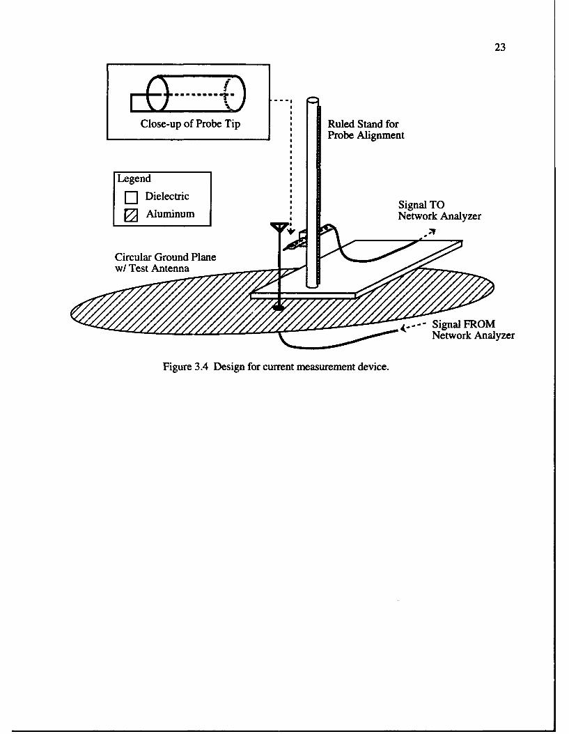
3.2.3 Current measurement (design only)

Although the design was never implemented, plans were drawn up for a device used to

measure currents along the physical structure of an antenna. The device shown in Figure 3.4

uses a probe with a vertically oriented receiving wire to measure E0 in the near field which is

proportional to the longitudinal current. By setting up the network analyzer for two-port

measurements, the field at the test location could be measured by viewing S2 1 . The probe

would be mounted on a mobile arm, which is, in turn, connected to a dielectric stand to avoid

electromagnetic interaction. By moving the probe along the structure, changes in the near field

(and therefore, current) could be determined. This type of measurement could be helpful to

support numerical analysis, or analyze coupling on structures that are not well-suited to analytic

modeling.

23

Close-up of Probe Tip Ruled Stand forProbe Alignment

Legend

L] Dielectric TOSAlumirnu Network Analyzer

Circular Ground Plane •°

w/ Test Antenna

....- Signal FROMNetwork Analyzer

Figure 3.4 Design for current measurement device.

24

4. LOW PROFILE BROADBANDING TECHNIQUES

4.1 Geometry

The impedance results for a linear monopole were seen previously. When operating

frequencies are as low as 2 MHz, as in our military vehicle application, resonance occurs when

a linear monopole's length is approximately 37.5 m, which corresponds to the V4 criterion.

Obviously, this would be unacceptable in a wartime environment since the antenna would not

only be quite immobile, it would also be terribly conspicuous to the enemy. By decreasing the

profile height, the antenna became more combat survivable and easier to implement on a

weapon system; however, the low frequency characteristics decreased accordingly. Therefore,

the objective of geometry alteration was to increase the length and volume of the radiating

structure while minimizing height. With this in mind, the limiting vertical height was set to 5.1

cm and geometry modification was attempted to improve the broadband impedance

characteristics. The 5.1 cm monopole had a V14 resonant point at 1.47 GHz, which is tawards

the high end of the 180 MI-Iz to 3 GHz band. This meant that radiation for the lower

frequencies suffers. Changing the geometry must not only lower this resonant frequency, it

must also be able to produce an omnidirectional far-field pattern throughout the frequency

band. This quality is important since the primary use for the antenna revolves around mobile

vehicle communication where most of the fields should remain relatively close to the horizon

without significant loss to higher elevations. Geometry alone controls the minimization of

profile height, but other mechanisms were necessary to avoid sacrificing other antenna

parameters. The structure also plays a major role in determining the directionality of the far-

field patterns.

4.1.1 "T" geometry

The first geometry alteration augmented the linear monopole by adding a horizontal

piece across the top. Figures 4.1 (a) and (b) show the dimensions of the linear monopole and

25

the "T" geometry variation. Although this design increased the effective length of the

monopole, the impedance was not significantly improved as Figures 4.2(a) and (b)

demonstrate. The added conductor surface helped the low frequency impedance match, but for

higher frequencies, the reactance excursions were more intense. In addition, current flowing in

a horizontal direction does not improve radiation in the vertical plane which is desired for the

received signal. Beyond this, since a monopole conductor produces a pattern with a null at the

tip, the T configuration generated a pattern that contained nulls along the transmission direction;

therefore, the design was not considered acceptable.

6.0 cm

5.1 cm 5.1 cm

(a) (b)

Figure 4.1 (a) Linear monopole (b) "T" configuration

4.1.2 2D and 3D kite geometries

The "Kite" Geometries, so-called due to their distinctive shape shown in Figure 4.3,

were merely variations of the linear monopole which included additional conducting material.

In the 2D case, arms are added to the structure in one plane. The 3D case combines arms in

two planes giving a more universally symmetric appearance. The reasoning behind this

geometry was to increase the amount of conductor while keeping the fields omnidirectional and

oriented in the vertical plane. The kite geometry follows the concept of a sparse conical mono-

26

500-5 0 0 .................. I ................. ------- --- ...... ...... I -• M . o I......

4 0 0 ...... ...i................. i ..r ... .i................. , ....... ......... •................. . ..............0 [ ZrMono]• , 0 0 ......... .... i .............. ....T ...... ..... I ............ ............ i ................. T................. SI Ui

lO0i .L Zr T "

300 ...... ., ...- +.-.

0 0.5 1 1.5 2 2.5 3 3.5Frequency (GHz)

(a)

2 0 . ............................. . .-. ............ ................ .... .................. ................. ...................

i/

I:. _ _

100 .... •..._

O ................ f................ . .r •T......... ... ........ i..... ......... ....• ' "• "' " ' ................. l

S-2 o o... ....... • + . - ----. Z_.

0 0.5 1 1.5 2 2.5 3 3.5Frequency (GHz)

(b)

Figure 4.2 Impedance comparison of linear and "T" monopoles:(a) resistance (b) reactance.

27

5.1 cm 5.1cm

(a) (b)

Figure 4.3 (a) 2D and (b) 3D "kite" antenna configurations.

pole. In theory, an infinite conical monopole antenna is frequency independent while a

truncated cone's frequency range is dependent on its size. The vertical height of the structure is

not the only important dimension; the cone angle also affects its performance. As the angle a

increases for the cone, the impedance variations decrease since less coupling occurs between

the arms [8]. Although the complexity of construction did not allow experimentation of the

angular phenomenon, a numerical analysis was conducted for the two-dimensional case and the

results are shown in Figure 4.4. In this study, a varies from 150 to 300 and 450 and results

match those expected. The impedances plotted in Figure 4.5 show that the increased volume of

the kite geometry resulted in significant reactance improvement for the low-frequency end

(from approximately -600 Q to around -350 Q2); however, in the upper portion of the

frequency range there was little difference between the kite and linear monopole.

4.1.3 Gamma geometry

It would appear that to increase conductor length without affecting the profile height, a

horizontal wire would be ideal. This is not the case however, because a horizontal conductor

would act as a transmission line which would be an inefficient radiator, and would not promote

28

2 0 0 .......... .... .... .....

cL=--1 50150 ..... - - -N E3Y ...

100

50/

0 0.5 1 1.5 2 2.5 3Frequency (GHz)

(a)

-50 a=5

0 ~ ~ ~ Z 0.a11.32 2.0Frequency..... ......

,4 -30 ....

(a rsitnc ()reaqtancy e.~

29

2 0 0 . ...............- .................. ....... I ....... ............Zr Mono

Zr2DKiteI /150 -------- Zr3D Kite.......................-----

c.J '1 i i100 -........ ' ff ... ...4... ....

'IN.0 ................ ..................... .. ....; .... ........ ................... .... .....................50 '

0 .

0 0.5 1 1.5 2 2.5 3 3.5Frequency (GHz)

(a)

10 0 ......................................................................... ................. :. ................... ................. .

S........ ... .......... ....• • ....... .... ......,10 0 .......... ........... ......

-2W .... _ .... . ..-2 0 . .. .;; .. .. . . . ... . . . . . . .. . . . .. ............... -................. . ............... i.................

--- ---i D Kite-400 ..... . - - ...... -. ................. .-5 0 0 .... ........... " .................. .............. .......... .......... ...... .......... ................. "-500-

-600

0 0.5 1 1.5 2 2.5 3 3.5Frequency (GHz)

(b)

Figure 4.5 Impedance comparison of a linear monopole andkite geometries: (a) resistance (b) reactance.

30

the vertically polarized signal desired. Since a pattern null appears at the tip of a monopole,

with this configuration there would be zero radiation in the direction of the line terminations

along the horizon, which is unacceptable for mobile ground communications. Therefore, in

another effort to increase the length of the conducting material without the efficiency and

pattern deficiencies, the linear monopole was bent to an angle 200 above the horizon with a

1.67 cm stub at the feed. This geometry shown in Figure 4.6 was labeled the "gamma"

antenna due to a slight resemblance to the Greek character, which increased monopole length

by 229%. This changed the X/4 resonant point from 1.47 GHz for the 5.1 cm linear model to

642.7 MHz for the 11.67 cm gamma. Bending the conductor allowed the increased length

without sacrificing in the E0 far-field. This model was appealing in that it had a simple form

and was not likely to resist vehicle movement when mounted properly. The impedance

characteristics are shown in Figures 4.7(a) and (b), which are also compared to the results for

the modified NEC model. As expected, the increase in length helped the impedance at low

frequencies; however, there were large variations after each resonant point. The design

becomes better matched for higher frequencies though. This design was closely examined with

different loading schemes.

3.43 cm

1.67 cm

K 9.40 cm

Figure 4.6 Gamma geometry.

31

1000

800 zr Measured

0 ........................... I ........... - NEC (Cap Load) .........

S600 ........................................

o 'I

400o II

0 -'---

0 0.5 1 1.5 2 2.5 3 3.5Frequency (GHz)

(a)

2 0 0 . .................. ... . . . . .................... ................. ................. ......................................

40 -.. . . . .. .

-60 ....

0 0.5 1 1.5 2 2.5 3 3.5Frequency (GHz)

(b)

Figure 4.7 Gamma antenna impedance, measured and computed:(a) resistance (b) reactance.

32

Despite the pleasing aesthetics of this design, the pattern was measured to be somewhat

weighted towards the extended arm at higher frequencies. Figures 4.8(a)-(l) contain a series of

radiation patterns for vertical polarization (E0) that spans the operating frequency range. On the

left side of the page, the patterns show ý cuts (side views) where 0 varies from 00 to 900 for

both 0=0O and 1800. The right side of the page has 0 cuts (top views) where 0=900 and 0

varies from 0 to 3600. Patterns for a particular frequency are listed next to each other and are

oriented according to an antenna bent to the left (along the positive x-axis). Not only is the

energy directed to the left at higher frequencies, but the pattern fragmentation creates nulls that

are unacceptable for a ground communication application. In addition, considerable radiation is

lost at the higher elevations which further deteriorates the low-elevation power levels. In order

to correct this problem, multiple gamma models were developed. It was thought that by

creating a symmetric geometry the design would inherit a more omnidirectional pattern and

better impedance values. These designs are described in the next section.

4.1.4 "Y" and "X" geometries

The multigamma approaches diagrammed in Figure 4.9 produced interesting results.

The first of these geometries was formed by adding a mirror image of the gamma in the same

plane as the original creating a two-arm antenna labeled the "Y." The second geometry

repeated the gamma shape every 900 forming a four-arm "X" antenna. The additions not only

balanced the symmetry of the antenna for pattern purposes, btit also increased the antenna

volume while increasing conductor length. The effect of the larger antenna size can be seen in

the impedance comparison plots in Figure 4.10. The larger the effective volume, the lower the

impedance amplitudes as expected by previous results. In order to see the positive effects of

the geometry on the radiation, an additional study was performed to compare with the results

for the gamma. The far-field patterns are organized in Figures 4.11 (a)-(l) where the Y antenna

restits are found on the left and the X antenna patterns are contained on the right. All plots

represent cuts with 0 fixed at 900. In each case, the antenna was situated with arms extending

33

1 1

0.8 0.8

0.6 0.60.4 0.4

0.2 0.20 0

0.2 0.20.4 0.4

0.6 0.6

0.8 0.8

(a) Phi Cut @ 0.5 GHz (b) Theta Cut @ 0.5 GHz

1 1

0.8 0.8

0.6 0.60.4 0.40.2 0.2

0 0

0.2 0.20.4 0.4

0.6 0.6

0.8 0.81 -1 -

(c) Phi Cut @ 1.0 GHz (d) Theta Cut @ 1.0 GHz

1 1

0.8 0.8

0.6 0.60.4 0.4

0.2 0.20 0

0.2 0.20.4 0.4

0.6 0.6

0.8 0.8

(e) Phi Cut @ 2.0 GHz (f) Theta Cut @ 2.0 GHz

Figure 4.8 Normalized radiation patterns for a gamma antenna: structure is alignedalong the horizontal axis with arm bent towards the left.

34

1 1

0.8 0.8

0.6 0.60.4 0.40.2 0.2

0 0

0.2 0.20.4 0.40.6 0.6

0.8 0.81 -1

(g) Phi Cut @ 2.0 GHz (h) Theta Cut @ 2.0 GHz

11

0.8 0.80.6 0.60.4 0.4

0.2 0.20 0

0.2 0.20.4 0.4

0.6 0.6

0.8 0.81 1

(i) Phi Cut @ 2.5 GHz (j) Theta Cut @ 2.5 GHz

110.8 0.80.6 0.60.4 0.4

0.2 0.20 0

0.2 0.20.4 0.4

0.6 0.6

0.8 0.811

(k) Phi Cut @ 3.0 GHz (1) Theta Cut @ 3.0 GHz

Figure 4.8(cont.) Normalized radiation patterns for a gamma antenna: structure is alignedalong the horizontal axis with arm bent towards the left.

35

18.80 cm

(a) "Y" Geometry

Z

(b) "X" Geometry

Figure 4.9 Extended Gamma Geometries

along the horizontal axis (and vertical axis for the X geometry) of the figures. Although the Y

antenna maintains a symmetric far-field pattern, radiation is not evenly distributed as 4 varies.

The X antenna develops a reasonable omnidirectional pattern throughout the frequency range.

Despite the far-field improvements, these antennas were too unwieldy for a battlefield mobile

communication system.

4.1.5 Antenna meandering

The concept of antenna meandering stems from the desire to increase conductor length

within a confined space. The process of meandering requires a linear structure to be folded

repeatedly to increase conductor length without a significant increase in antenna volume. Two

meandered geometries were examined, and are pictured in Figures 4.12(a) and (b). The first

merely wraps a linear monopole back towards the ground plane. The second meander takes

place in the plane of the angled arm of the gamma geometry. The problem with these

meandering geometries was that coupling occurred between adjacent conductors. Therefore,

low-frequency improvements were overshadowed by the interaction of closely spaced antenna

36

7 0 0 ..........I.... ......

600 ........ Zr Gamma-- zr"V"Geometry1_ 00 Zr....... xX" Geometry ......

400 .... ...... ---

00 0.5 1 1.5 2 2.5 3 3.5

Frequency (GHz)

(a)

400 ................ .. ................

300 - 1----- Zi GammaA -Za V" Geometry200 L......... ...... ..... .. = r .......

0....... i "X eoer

-200/

0 0.5 1 1.5 2 2.5 3 3.5Frequency (GHz)

(b)

Figure 4. 10 Measured impedance comparison between gamma, Y, and X geometries:(a) resistance (b) reactance.

37

1 70.8 0.80.6 0.60.4 0.40.2 0.2

0 00.2 0.2

0.4 0.4

0.6 0.60.8 0.8

(a) Y@O0.5 GHz (b) X@O0.5 GHz

0.8 0.80.6 0.60.4 0.40.2 0.2

0 SC00.2 0.2

0.4 0.4

0.6 0.60.8 0.8

1 1

(c) Y @1.0OGHz (d) X @1.0OGHz

0.8 0.80.6 0.6

0.4 0.40.2 02

.0 0.

0.2 0.2

0.4 0.4

0.6 0.60.8 0.8

(e) Y @1.5 GHz (f) X @1.5 GHz

Figure 4.1 1(a)-(f) Normalized radiation patterns for Y (left) and X (right) antennas:structure is aligned along the horizontal axis.

38

1 10.8 0.80.6 0.6

0.4 0.40.2 0.2

0 0

0.2 0.2

0.4 0.40.6 0.60.8 0.8

11 -

(g) Y @ 2.0 GHz (h) X @ 2.0 GHz

1 1

0.8 0.80.6 0.6

0.4 0.40.2 0.2

0 0

0.2 0.2

0.4 0.4

0.6 0.60.8 0.8

1 -1 -

(i) Y @ 2.5 GHz (j) X @ 2.5 GHz

1 1

0.8 0.8

0.6 0.6

0.4 0.40.2 0.2

0 00.2 0.2

0.4 0.4

0.6 0.60.8 0.8

1 -1 -

(k) Y@3.0GHz (1) X@3.0GHz

Figure 4.11 (g)-(l) Normalized radiation patterns for Y (left) and X (right) antennas:structure is aligned along the horizontal axis.

39

y8.4 cm

10m 1.0 cm

1.0 cm z

5.1 cm } 1 5.1 cm

(a) linear meander (b) gamma meander

Figure 4.12 Meandering geometries

wires, which resulted in large variations in resistance and reactance for both models. Although

the meander was not further examined, the geometry in 4.12(a) led to the development of the

folded gamma antenna that was eventually chosen for the application.

4.2 Lumped Loading

Variation in geometry alone was not enough to develop a broadband antenna design for

a low-profile, vehicle communication system. Therefore, emphasis switched to the application

of lumped loading schemes to improve antenna performance. In Chapter 2, the high frequency

response of lumped components was examined, and due to the great variation of the impedance

of reactive components, research was limited to the analysis of resistive loading. It has been

determined that by inserting a resistor a distance of V/4 from the tip of a monopole, it can be

terminated in its characteristic impedance which minimizes reflections from the end of the wire.

More specifically, the addition that a 240 Q• resistance improves impedance characteristics by

causing a large traveling wave to exist simultaneously with a small superimposed standing

wave on the wire (9]. Using the lumped loading technique described in Chapter 2, various

loading configurations were attempted with the geometric modifications discussed previously.

40

4.2.1 Resistive series-loading

The first loading configuration implemented Altshuler's technique [9]. The addition of

a lumped resistive load in series with the antenna structure can improve the impedance

characteristics. A diagram of the lumped loading system applied to the gamma geometry is

shown in Figure 4.13.

3.43 cm2 0 o1.67 cm

K 9.40 cm N

Figure 4.13 Lumped loading implementation.

For an impedance comparison, the load values were varied from 5002 to 240 Q, and

graphed in Figure 4.14. In each case, the impedance improved as the resistance increased, and

the response was optimized with a 24002 resistor as expected from the literature [9]. Although

the impedance amplitudes decreased, the low-frequency reactance was unaffected. In addition

to this, the inclusion of the resistance decreased the efficiency of the radiated power since some

was lost in the component. These losses, however, may be acceptable if the resulting

impedance is made more easy to match to the generator system. Since the impedance match

allows more energy to reach the antenna, this may account for the loss by the loading system.

To solve the reflection problem for low frequencies though, it was necessary to implement a

different resistive loading technique as described in Section 4.2.2.

41

8 0 0 -...------- ...............- ................. ................. ................... ................... I..................7 0 -........ ]•............... ..... . ..... ................. Ti... . ...... i............... !................800----I.... . .......

60 ............... ........... .... ...............[ I • G-O--ma I.........700600 - ZrGamma I Q

500 ................ ............... ............... ------. ZrG am m a 10 0 ......... "i mI1........... Z5o a I Q

4 ............... ............ - -- ZrG ammx a240 Q .........

4 0 0 .......•k.o ............... ............ ................ i .................. ? ................. i.................. .........200100-

00 0.5 1 1.5 2 2.5 3 3.5

Frequency (GHz)

(a)

400 ................ : .................. :"................ 1 G m a-.........."

400 Zi Gamma 50Q

200 - Zi Gamma 150 f

0- Zi Gamma 240OQI 0 0 ~ ~~~.. ........... ........... .............,. .. . .,.

0-loU 100 ......

-2Wo

-300--400

-500 I . .. . . . . .

0 0.5 1 1.5 2 2.5 3 3.5Frequency (GHz)

(b)

Figure 4.14 Measured impedance comparison for lumped loaded gammageometry: (a) resistance (b) reactance.

42

4.2.2 Resistive tip-loading

Another lumped loading scheme analyzed in the laboratory consisted of connecting a

resistive load from the monopole wire termination to the ground plane. In essence, this

converted the gamma geometry into a loaded loop, which removed the problem of significant

reflection especially at the lower frequencies. Tip-loading did not affect the higher frequency

response where the impedance match was already acceptable. The loading technique is

diagrammed in Figure 4.15 for the gamma antenna, and was easily adjusted for multiple

gamma structures. In order to see the optimization of the 240 0 resistance, each model was

tested with a number of loading values. Figures 4.16-4.18 show the results for various load

resistance values.

3.43 cm

200 LumpedJ Load

1.67 cm

9.40 cm

Figure 4.15 Resistively tip-loaded gamma antenna.

As expected, the impedance excursions were minimized with a load resistance of 240 Q"

since the characteristic impedance was most closely matched just as in the other loading

examples. Also, the increased conductor and antenna volume had the same positive effects as

before. It should be noted that the advantage of these loading systems to the series resistances

experimented with earlier focuses on the lowest points of the frequency range. Comparing the

reactance characteristics of the series-loaded gamma with the tip-loaded gamma for 180 MHz,

43

the value has decreased from approximately -300 Q to -80 Q. This fact increases the matching

potential of the second design over the first. Impedance matching will be discussed in Chapter

5. Because the Y and X geometries were too complex and space intensive, work progressed

on simpler improvements of the 240 Q1 tip-loaded gamma.

For a closer look at the impedance of this design, refer to Figure 4.19. Notice that

despite the error in the resistor-only simulation in Chapter 2, when implemented on the

antenna structure, the model follows measured data well. This demonstrates the utility of the

parasitic capacitance modification and detailed geometric computer modeling for accurate

simulation of antenna characteristics. Emphasis then changed to methods of antenna

construction and the appearance of the far-field pattern.

In terms of mechanical realization, the tip-loaded gamma antenna presented some

difficulties. First, the structure had two contact points with the ground plane which increased

the surface area necessary for mounting. Secondly, the bend required reinforcement due to the

size of the operational system and desire for a flexible arm. Next, the load resistor would have

to be shielded. One method for accomplishing this included placing a grounded sheath over the

loaded wire, a second method called for tubular antenna structure to allow the load to be placed

within the conductor with a path to ground at the feed location. The experimental results of

these investigations showed significant impedance degradation; therefore, these methods were

not used.

The radiation of the unloaded gamma antenna was heavily weighted towards the

direction of the extended arm; with the resistive load included, the pattern results were further

degraded. Since the extended gamma geometries were discounted due to space considerations,

smaller structural changes were attempted. The meandering linear monopole from Figure

4.12(a) was equipped with a tip-loaded resistor. This antenna required minimum volume and

showed excellent omnidirectional characteristics; however, the efficiency of the small structure

was found to be too low for the limited power supplies used in mobile communications.

Numerical experiments were performed to do determine the effect of increasing the space be-

44

8 0 0 ..................................................... ..................................................................

700

600 Gamma50 ..- 0100

~500 -----. l..o-----------: ...... --7 Garma 150i Q ......

400 1~Zr Gamma 240mQ

~3 0 0 ----.. .---------

200

100 ----

0 .. .

0 0.5 1 1.5 2 2.5 3 3.5Frequency (GHz)

(a)

4 0 0 . ................................. ..... ............... ........... ------- ............. ........ ............. ....

2O00

, -2 0 0 ................. - .............. ................. .................. .................. ................. ................. •

i- ----- -i Gamma -100 ----400 K ....... 10

-- -ZiGamma 240 I

0 0.5 1 1.5 2 2.5 3 3.5

Frequency (GHz)

(b)

Figure 4.16 Measured impedance comparison for a tip-loaded gamma:(a) resistance (b) reactance.

45

5 0 0 ................... .... ............................................................. ................... .................. ..400

vr loo00200 v240 53 0 0 i ~................ ........ ,.......... ,. ........-

-S2 0 0 ...... .. ................ .................... ................. .................... i.................. •.................

10 0 ...... ............ ... ;. ...... i ..... ......... ... ...................

1000 . . I . . . I . .I . . . . I . . . I . .

0 0.5 1 1.5 2 2.5 3 3.5Frequency (GHz)

(a)

10- .....o. ......... ........ .... .................... ................. ---------------- ................. "

20 0 ........ ..... .. .........

.. .Zi V 240 Q~- 3 0 . . . ' . . . .. ' . ..... . . . ... i.. . . i . . . .... . .... .. .

1200 ........ z 10L

0 0.5 1 1.5 2 2.5 3 3.5Frequency (GHz)

(b)

Figure 4.17 Measured impedance comparison for a tip-loaded Y:(a) resistance (b) reactance.

46

3 0 0 .......... ...... .. 7 ................ 1- ............. ....... ........ ............ ........................

[ ZrX 50 Q250 ....... . . Zr X 240 Q .......... .............

2 0 ........ ................T ................. i...............: ........... ................. ................... . ...... ....... ... .......... .. ........ L . ....... ........

~ 50 .

1 0 . . . i . . . . . . i . . ... . . . . . .. . . .... .....

0 0.5 1 1.5 2 2.5 3 3.5Frequency (GI-z)

(a)

.. .-Z i X 5 . .-e 0i 2000 . . . . ' . .... i. . . .- .. ... . .. .

0 0.5 1 1.5 2 2.5 3 3.5Frequency (GHz)

(b)

Figure 4.18 Measured impedance comparison for a tip-loaded X:(a) resistance (b) reactance.

47

300 ........-.................. ...... .... - 6-- Zr M easured- -Zi Measured200 . ... .. ......... .................. ................................--........... 0 - Zi N E C d,,,• •-- -0 ZrNEC

10-S..... ........ .. . ....... . .. .. . .. .

0 .. ............... J .................. .................. i................. i.......................... .. . ................oi

-30 0 . . . ' . . . . . , , . . . . . . . .

0 0.5 1 1.5 2 2.5 3 3.5

Frequency (GHz)

Figure 4.19 Measured impedance of a 240 Q2 tip-loaded gamma antenna andcorresponding NEC analysis: (a) resistance (b) reactance.

tween conducting wires to minimize coupling. It was determined that by extending the arm

farther away from the feed, the impedance amplitude decreased. To maximize the effects of the

current distribution on the antenna and create a strong E0 pattern, it was desired to havu a

vertical conductor at locations where feed current would be the highest. The conductor

separation distance was kept large to minimize coupling. At the same time, by forcing the feed

and monopole termination to be in close proximity, the mounting area could be minimized. By

folding the monopole into a triangular configuration, it was possible to develop a self-

supporting structure with promising performance values. This geometry led to the folded

gamma antenna which became the operational design. Figure 4.20 shows the progression of

the folded gamma design. The third antenna includes a curved comer to make the structure less

likely to be hung up on obstacles. This geometric modification did not seriously affect either

the impedance or the pattern characteristics of the antenna.

48

1.0 cm 5.0cm 5.0 cm

4.0 cm 4.0 cm 4.0 cm

1.0 cm 1.0 cm 1.0 cm

Figure 4.20 Progression of the folded gamma geometry.

The measured impedance of this design is compared to those for the tip-loaded gamma

model in Figure 4.2 1. Figures 4.22(a)-(f) show a series of far-field 0 cut patterns for both the

tip-loaded gamma and folded gamma designs. These patterns are normalized to the maximum

value of both antennas in order to have a radiation comparison for each frequency. The solid

lines represent the tip-loaded gamma results while the dashed curves show the folded gamma

far-field patterns. Notice that throughout the frequency range, the folded gamma maintained a

relatively omnidirectional pattern. On the other hand, the tip-loaded gamma antenna radiation

was dominant to the right (away from the lumped load) for low frequencies, but the pattern

flipped to the left and fragments as frequency increased. Therefore, the folded gamma appears

to be well suited to a mobile ground communication system.

4.3 Grounded Sleeves

Aside from the geometric alterations earlier conducted on the antenna, experimentation

was also accomplished with the use of grounded sleeves for impedance improvement. As

described in Chapter 2, sleeve structures were more easily constructed and measured in the

laboratory than modeled on a computer. The sleeve model was realized by placing a

conducting cylinder concentrically over the test monopole and attaching it to the ground plane.

Sleeve length was varied in the laboratory based on fraction of the center monopole length.

49

300 .--- Zi Loaded Gammai •, -- -- Zr Folded Ga m

2- 0 0 ... ........ ............ ..........

' Fode Gamma

10 ................. .......... ........ ..... ............ • ............ ..... ... ............. ............ , .-. • . ........... ..

_,o ................ ...L...._..... , ............. ................. .................. ..........74........ • ............... .- 10 0 ..... .. .... .... ... ....... ------ -....... .... .... i.....................

-2000 0.5 1 1.5 2 2.5 3 3.5

Frequency (GHz)

Figure 4.21 Measured impedances of a 240 Q tip-loaded gamma and a folded gamma.

400 ............. ............. .."" ..................... .- - z~ ~asm~a u e !...... ................. .......... .........

3(j() -h -6 Zr Measured

3 0 0 . ............... ...0 .. .... I....... ; ................... . ...... . ................... ...................

200- O~ZrNEC-~-- Zi ZNEC

" -10 0 .... • ----:•':-i ....... \- . ....... ......•-• '-; - -.............. ............ .::( -:-:: -..i.........

-2 0 0 ...........- .... ............... ."•....................... ................. ................. .................. .................

-300 .. . . . . . . . . ..

0 0.5 1 1.5 2 2.5 3 3.5

Frequency (GHz)

Figure 4.21 Measured impedance vs. NEC analysis for a folded gamma.

50

7 70.8 -0.80.6 0.6

0.4 0.4

0.2 0.2

0.2 0.2

0.4 0.4

0.6 0.6

0.8 0.8

I L

(a) 0.6 GHz (b) 1.0 GHz

0.8 0.80.6 - o 0.60.4 , 0.4

0.2 a 0.2

0 0

0.2 0.2

0.4 0.4

0.6 0.6.6

0.8 0.8SI-

(c) 1.4 GHz (d) 1.8 GHz

I I0.8 0.80.6 % 0.6 -0.4 0.6

0.2 0.2

0 00.2 •/0.2

0.4 -0.4

0.6 0.6

0.8 0.8I - I

(e) 2.2 GHz (f) 2.6 GHz

Figure 4.22(a)-(f) Radiation pattern 0 cuts for a loaded gamma (solid line) anda folded gamma (dashed line).

51

The measured results for varying sleeve length appear in Figures 4.23(a) and (b). The

addition of the sleeve helped the low-frequency characteristics, but as sleeve height increased,

the performance at high frequencies decreased. Therefore, the grounded sleeve seems to be

useful for impedance improvement across a certain band of frequencies, and its height will

determine which range is applicable.

In another experiment, short sleeves were excited to realize a two-antenna system for

low and high frequencies with omnidirectional radiation patterns. It was thought that sleeves

of varying heights could be positioned concentrically to create a multiband antenna system.

The physical models failed to develop a horizontally dominant radiation pattern due to coupling

with structures inside the sleeve. The array analyses in Section 4.4 provided the explanation

for this. The scalloped radiation pattern was due to the small sleeve radius. For more

information about grounded sleeves and excited sleeves see the literature [4].

4.4 Arrays

The final concept for broadbanding that was experimentally analyzed dealt with the

combination multiple antennas in arrays for multiple band transmission. The design originated

with the examination of two linear antennas placed next to each other, a long monopole for low

frequencies and a shorter version for a higher band. Radiation patterns measured in the

laboratory showed that although the large monopole was negligibly affected by the presence of

the smaller one, the inverse was not true. The smaller antenna could not seem to radiate

through the low frequency monopole due to coupling. A simple solution to this called for the

addition of a duplicate antenna on the opposite side of the large radiator to balance out the

pattern. This operation succeeded, and experimentation of this configuration led to the

determination of a subtle relationship between adjacent radiators. Since the amount of coupling

between two antennas is indirectly proportional to the distance between them, increasing the

separation distance causes less performance degradation. With the third antenna included,

however, the analysis became much more complicated. Figure 4.24 details the geometry of the

52

5 0 0 ......... ....... ----..... ----- -----

Zr no sly400 ...... Zr .2slv ....

-- - - Zr .3 slv

Ci --- 0....Zr .4 slv

300~~ -~Z.sIvU -*---Zr.7slv

.4 ~ ~ p...... .......... L ........ ................... ... ........200

100

0 .~-' . ..

0 0.5 1 1.5 2 2.5 3 3.5Frequency (GHz)

(a)

Zi Mono300 - Zi .2 sIv ----I.........

- - -- Zi.3 slv200 ----.Zi .4 sIV

100 ------ Zi .5sIv

-3004

0 0.5 1 1.5 2 2.5 3 3.5

Frequency (GHz)

(b)

Figure 4.23 Measured impedance of variable height grounded sleeves:(a) resistance (b) reactace.

53

1.0 cm

T 0

II *o 17.5 cm o 3.0 cm

o @1.5 cm

(b) Top view of five-element system

(vertical monopoles arranged in a diamond)

(a) 1.0 cm

Figure 4.24 Array Systems (a) three-antenna system

(b) placement of five-antenna system.

three-antenna system. The center conductor measured 17.5 cm and operated at low frequencies

since it resonated around 428 MHz. The smaller monopole had a 3.0 cm height which

corresponded to a 2.5 GHz resonance. For arbitrary applications, these heights can be

determined by the engineer for particular frequency bands.

Therefore in order to develop a system, after choosing monopole lengths, the only

parameter to set is the separation distance. Coupling of the large antenna resulted in large

amounts of power to be radiated at higher elevations. Because this was not acceptable for a

ground communication application, the separation distance was increased to minimize these

effects. Since the coupling is inversely proportional to the distance, it would appear that a large

separation would be optimum. However, the problem presented with a large distance between

elements deals with the 0 cut pattern lobe generation as described in the literature [10]. As the

array elements move apart, the omnidirectionality of the pattern decreases. Therefore, the array

combination had to be designed such that minimal coupling occurred with maximum

omnidirectionality, a trade-off between wide and narrow separations. As elements become

54

shorter for higher frequency, the separation distance must decrease accordingly. Once an

acceptable design in two dimensions was complete, a third set of monopoles was added to

operate at even higher frequencies with 1.5 cm height in order to resonate at approximately 5

GHz (see Figure 4.24(b)).

The question then arose about how to terminate nonexcited elements while radiating on

a certain channel. A graph of the segment currents with the midband monopoles excited is

shown in Figure 4.25. The other antennas were terminated with an open, short, and matching

load to determine the minimum coupling current configuration. From this we determined that

the nonradiating monopoles should be shorted to ground during operation. Following the

current analysis, the radiation patterns for the antenna systems are presented in Figures 4.26-

4.27. For the most part, the power remains close to the horizon with a reasonably

omnidirectional distribution.

0.05 -------------------- ........... CenterOpen -- f-- High Openi- 3 - Center Short - - High Short

0.04 . ...................... Center Matched --- f-- High Matched

S0.02S0 .0 3 ~ ~........ ......... •..................... ;............ ...... ..................... * ................ . .................

Q.\ .. .. .....

0 .0 1 ........... .................... ........... C

..... I. . . . . . 1..., ,..

0 0.2 0.4 0.6 0.8 1 1.2Vertical Distance (m)

Figure 4.25 Segment currents on five-antenna system: midrangemonopoles excited.

55

1 1

0.8 0.8

0.6 0.60.4 -0.4

0.2 0.20 0

0.2 0.20.4 0.4

0.6 0.6

0.8 0.81 -1--

(a) Array Phi Cut @ 3.0 GHz (b) Array Theta Cut @ 3.0 GHz

1 10.8 0.80.6 0.60.4 0.40.2 0.2

0 0

0.2 0.20.4 0.40.6 0.6

0.8 0.811

(c) Array Phi Cut @ 4.0 GHz (d) Array Theta Cut @ 4.0 GHz

1 1

0.8 0.80.6 0.60.4 -. 40.2 0.2

0 00.2 0.20.4 0.4

0.6 0.6

0.8 0.8

(e) Array Phi Cut @ 5.0 GHz (f) Array Theta Cut @ 5.0 GHz

Figure 4.26 Radiation patterns for five-element antenna system: midrangemonopoles excited, others shorted.

56

1 1

0.8 0.8

0.6 0.60.4 -0.4

0.2 0.20 0

0.2 0.20.4 0.4

0.6 0.6

0.8 0.81 1

(a) Array Phi Cut @ 6.0 GHz (b) Array Theta Cut @ 6.0 GHz

1 1

0.8 0.8

0.6 0.60.4 0.4

0.2 0.20 0

0.2 0.21.4 0.4

0.6 0.6

0.8 0.81 1 -

(c) Array Phi Cut @ 7.0 GHz (d) Array Theta Cut @ 7.0 GHz

1 1

0.8 0.8

0.6 0.60.4 0.40.2 0.2

0 0

0.2 0.20.4 0.4

0.6 0.6

0.8 0.81 -1 -

(e) Array Phi Cut @ 8.0 GHz (f) Array Theta Cut @ 8.0 GHz

Figure 4.27 Radiation patterns for five-element antenna system: high-rangemonopoles excited, others shorted.

57

4.5 Broadbanding conclusions

In this chapter, various methods of broadbanding were examined. Each of the methods

was measured in the laboratory, most of which were also analyzed using NEC. From the

systematic refinement of geometry and loading, a folded gamma antenna was developed that

meets the design specifications for a low-profile, broadband, monopole vehicle antenna for use

in mobile ground communication. In addition to this, the use of grounded sleeves and array

combinations was viewed for their application to the broadbanding process.

58

5. MATCHING NETWORK GENERATION

The ability of an antenna to radiate optimally depends on numerous factors. One very

important radiation parameter deals with the impedance mismatch between the antenna and its

source. Using a transmission line analogy from basic electromagnetics, changes or

discontinuities in impedance cause signal reflections as a wave propagates down a line. The

reflections lead to interference which decreases the quantity of the signal that is actually

transmitted over the line. The same is true in an antenna system; regardless of the device

design, these achievements could be useless if the antenna is not properly matched to its

source. Therefore, the problem is to develop a lossless network that makes the impedance

"seen" by the generator equal to that of the generator itself. By equating these two impedances,

the power delivered to the antenna for radiation is maximized.

5.1 The Real Frequency Method

The Real Frequency Method (RFM) developed by Carlin [ 11] seeks to determine the

circuitry necessary to maximize the power transfer from a generator to an arbitrary antenna.

The key advantages of the RFM over those for previous matching networks theories are that

there are no assumed models or analytic expressions necessary for the load. In addition, no

assumptions are made for the form of the system transfer function. Figure 5.1 shows a block

diagram of the matching network system. In the figure, ZL represents the impedance of the

antenna and Zq is the matching network impedance that maximizes the power delivered to the

Rg

Vg Matching Z

Network

Zq

Figure 5.1 Diagram of matching problem.

59

load. To quantify the power interaction between the generator and the load, the Transducer

Power Gain (TPG) is used. The TPG is defined as the ratio of the power delivered to the load

to the power available from the generator. More specifically, it is given by

T(0)2) = Power to Load = P

Power Available from Generator P.

(5.1)

4Rq((O)RL (o)

t)) + Z(O)I

This is not a trivial problem because the impedance is a frequency-dependent complex value.

However, there is a Cauchy-Riemann relation between the real and imaginary parts of analytic

functions which simplifies the task. In addition, if the analytic function does not contain any

poles that reside on the j0o axis, the real part completely determines the imaginary part for all

frequencies and vice versa. The following equations show how the resistance and reactance

values are related

Z(to) = R(w) + jX(ao) (5.2)

R(co) = -L fY dA +R(-) (5.3)

xLZ-co(5.4)

X(CO) = I "-- a R()(54ir f - o .

By assuming the function has no poles on the jo axis, we develop what is known as a

minimum-reactance function, which means that by determining only the resistance of the

impedance function, the reactance is also automatically determined. Therefore, the computation

time is reduced by half. It should be noted that the explanation of the RFM that follows is a

condensed version of information found in the literature [I 1]-[12]. For a more detailed

derivation, the reader is directed to these sources.

The first step in the RFM is to take the frequency range of the antenna design and

discretize it into a series of matching frequencies 0<0o1<o02<0)3<...<(On. Knowing the

antenna impedance at these points, it is necessary to determine Zq to maximize the TPG in (5.1)

60

for the entire frequency range. To take advantage of the impedance relation, the values of the

resistance Rq are split into a number of linear segments so' that it can be realized by the

following summation

N

Rq((o) = ro+ 1.a,((O)r. (5.5)k=i

where ro represents the dc resistance of the system. To make the summation copy the form of

the resistance function, the values of ak(o)) are determined by a step function

ak = (5.6)0 Ok <5 0

and the rk's are a series of slopes that represent the resistance curve. By finding the set of

slopes that optimize the TPG function, a piecewise linear impedance function is developed for

the matching network. Using the impedance relation from (5.2)-(5.4) the reactance can broken

up similarly by

N

X'(0o) = a k (C)O (5.7)k=1

which uses the same values for the rk's, and the bk's are found by the integral

bk = ln Y+ody (5.8)b i= (wok -04O-1),- 1 Y - O

which can be evaluated in closed form by

"C[2ok ln(2cOk) - (2a.k - A) ln(2 (Ok - A) - A In A ]k

bk C[(20Ok - A)ln(2cOk - A)- 2 (o.k - A)ln2(wok - A) - AlnA] (o=(okI

C[(Ok - w) ln(o•k - (0) - (0)k-1 + o) ln(0Ok-1 + (0) otherwise

+ ((ok-w - w)ln I wo- cok-1 I-(wOk -o)ln I co- o, I

C = I A = 0)k - 03k-1 (5.9)KrA

Once the piecewise linear curve has been determined, the RFM requires that the

piecewise linear curve is approximated by a rational function. Using a rational function in the

61

form of (5.10) leads to an impedance function that can be realized in a two-port cascaded

circuit.

A o)'Rq = Ac(.101 + B 2 + B0), +'"+B 2. (5.10)

From the rational resistance function, the roots of the denominator are found. Retaining only

those that reside on the left-half of the plane, a polynomial can be formulated with those roots.

This polynomial becomes the denominator of the impedance function.

Q(S) = Is + (r, + Ax)]s + (r, - jx)] ... [Is + (r. + jx.)][s + (r. - jxA) 5.1

We assume that the numerator of the impedance function has the same form as Q(s).

Zq = a.-.s+a. (5.12)

Q(s)

This equation can be broken up into even and odd parts of both the numerator and denominator

which, in general form, is

e, (s) + o. (s) (5.13)

e, (s) + od (s)

Since the rational resistance function is known, equating even and odd parts allows us to solve

for the an coefficients.

= e. (s)ed (s) - o (s)od(S) (5.14)

ed(s) - od(s)

We are left with an impedance function that is a quotient of polynomials that can be realized in

circuit form.

Zq = a(s) (5.15)

Q(S)

This quotient of polynomials undergoes long division to generate forms resembling (5.20)-

(5.21). Each value must be normalized with respect to the operating frequency so the

component values must be scaled by an appropriate factor.

62

5.2 Computer Implementation

Two methods of computer implementation of the impedance matching process were

examined. The first followed the method described earlier, while the second represented a

modification of this method and has not been fully developed.

5.2.1 Implementation of the real frequency method

For computer implementation, FORTRAN was chosen due to its complex mathematics

ability along with the availability of subroutines for optimization [13]-[15]. The Real

Frequency Method was easily adapted to the computer, and the algorithm followed the same

three phases as described in Section 5.1. In the program, match.f , the user is asked to

identify the input data file which contains the discretized impedance information of the arbitrary

antenna. The data file is organized as a listing of resistance, and reactance for each testing

frequency. The user is then asked to enter the frequency units and dc resistance along with the

frequency range to be examined. The program presents a list of the input data points allowing

the user to select the matching points from the list for the optimization routine. This feature

allows variable discretization and the definition of subranges. The user then has the option of

weighting the optimization of each matching frequency. This initializes the first optimization

routine. For this approach, a subroutine using a Levenberg-Marquardt algorithm optimized the

expanded TPG equation given by

4RL (w•),r + yak (O))rk

T(O) = + (5.16)

RL(w) + r N + [a()rk + XL (O)+Ibk(CO)rkIk=l k=l

by solving for the values of the rk's that minimize the error function.

N 2

E = [I[- T(ak)] (5.17)k=1

63

The second step was to approximate the piecewise linear curve by a rational function.

To simplify the calculation of the coefficients, the values were normalized with respect to o2

and inverted giving the polynomial

Rq= Co +C'C +c Co4O +... +C. (5.18)

whose function values and derivatives are easily calculated. Since the resistance function

should be positive for all o, this is tested by the program, and the value of the constant term is

kept positive to ensure a finitt positive starting point.

After determining the rational function, the program solves for the roots of the

denominator, finds the left-hand-plane roots, and multiplies the roots to create the denominator

of the impedance function. Knowing the denominator, the coefficients of the numerator are

evaluated by using a matrix subroutine to solve the system of equations given by taking the real

part (resistance) of the impedance equation and equating the numerators of (5.10) and (5.14).

The equations form a diagonally filled matrix in the form

±Q, ±Q3 ±Q5 ... 0 0 0 a, 0

0 -_Q2 T .Q 0 0 0 a2 0

0 ±Q, ±Q3 ... 0 0 a3 0

(5.19)0 0 ±QI ... ±Q- 2 ±Q 0 a.- 2 0

0 0 0 .. Q•-3 F•Q, 1 0 a.-, A

0 0 0 ... t±Q.- 4 ±Q.-2 ±Qf an 0

Now that the values for all coefficients of the impedance function are known, the

problem turns to circuit realization. Due to the method of formulation, the numerator will

always be of one order less than the denominator which allows for different forms of

realization. Given this form, Darlington [16] has shown that any positive-real function (e.g.,

resistance) can be realized as a cascaded LC circuit terminated with a resistance. Both circuit

realizations are developed by performing long division of the impedance function. The first

method consists of a fraction expansion about infinity which would have the general form

64

1Z' (S) =I(5.20)

C, +

C2 + 1+

The second method removes a term and then continues with an expansion about infinity

Zq(S) = 1 1 (5.21)

-- +C2 +1

L2 (2+--

Of course, the size of these long divisions and, consequently, the number of components

necessary to realize the circuit, varies with the order of the rational function used to

approximate the piecewise linear curve. The orientation of the circuitry components goes from

the antenna on the left side of the equation to the generator at the right. Skeptics will point out

that the resistance found closest to the generator does not comply with the desire for a loss-less

network. This, however, can be realized by placing a transformer between the generator and

the matching network. In order to realize a circuit, the values contained in the cascaded fraction

must be normalized to the testing frequency unit.

Two versions of the program were produced. The first code utilized IMSL [141

routines available on the University of Illinois CONVEX main frame. The desire to generate a

portable program with operational control of the subroutine parameters led to a second version

which was written using subroutines from Numerical Recipes [15]. Table 5.2 lists the

subroutines and uses for both codes. The optimization routine in each case used a Levenberg-

Marquardt algorithm for minimization. This method is based on using a steep descent method

with points far from a minimum, and switches to an inverse-Hessian method as the guess

approaches the minimum. Although the methods were the same, the Numerical Recipes code

required the formulation of the derivatives to be supplied which seemed to decrease

computational time. In addition, IMSL optimization was limited by user-defined maximum

65

number of iterations, which if exceeded caused program termination. The Numerical Recipes

subroutine allowed a more subtle alternative for cases that did not seem to converge.

Table 5.1 Listing of computer subroutines used in the impedance matching program.

Purpose IMSL Numerical Recipes

Optimization DUNLSF MRQMIN

Root Finding ZPLRC ZROOTS

Matrix Solution DLSARG LUDCMP

5.2.2 Implementation of the modified real frequency method

Although work continues on this form of implementation, results look promising at this

time. The modification of the RFM removes the requirement for two optimization loops by

optimizing for the impedance function directly. By generating an array of coefficients, the

impedance function can be written as

Z(s) = gSdeg-1 + + A2s + A.= e (5.22)

A2 &ggSde +... + Adg+ 2 S +Adeg+i

where deg indicates the user-defined resolution of the impedance function. These coefficients

are chosen to minimize the error function in (5.17). By utilizing this modification, the separate

calculation of linear and rational functions is avoided and the subroutines for root finding and

matrix solving are not needed. Therefore, this method is advantageous not only because one

optimization loop yields a realizable circuit, but also because both the resistance and reactance

are optimized simultaneously. In the Real Frequency Method, the rational function

optimization dealt with the resistance function alone. The reactance was determined from the

solution of the impedance function coefficients. The reactance value was therefore removed

from the optimization process. Differences in the linear and rational reactance functions can be

significant, which lead to problems in the realization of an impedance matching network.

66

Section 5.3.2 shows a case where the failure to optimize the reactance value yields poor TPG

results.

Three problems were encountered when implementing the modified system. First, the

derivatives for the TPG function in terms of the impedance function coefficients were

extremely complex. Therefore, a finite difference method was implemented to solve for each

of the derivatives. Next, the problem of optimizing to a local minima was noticed. To solve

this difficulty, the initial guess for the minimization routine was randomly chosen for multiple

trials. The best result of these trials became the final optimization. The final difficulty dealt

with the impedance function coefficients. The optimization routine was modified to force each

coefficient of the function in terms of s (where s -> jo) to a positive value. This insured that

the output function could be realized by a matching network. Some preliminary results are

included in the following results summary.

5.3 Computer Results

The computer results for the impedance matching program have been mixed. For

some antenna geometries, the TPG has increased appreciably across the entire frequency range

tested. At the same time, some antenna geometries were ill-conditioned for the subroutines,

which forced the research towards developing improved techniques to implement the Real

Frequency Method for arbitrary antennas.

5.3.1 Resistively loaded linear monopole

The first test case was originally tested by Ramahi 1121 which served as a TPG

comparison. The test antenna was a 12 m monopole with a 7.5 cm radius and had a 240 U1

series resistance placed 6.9 m from the base. The size sets the resonance at 625 MHz, but the

impedance match was desired for 2-9 MHz. Therefore, the antenna measured approximately

0.32 X at the lowest testing frequency. Impedance values for the antenna shown in Figure 5.3

were loaded into the program. After the first optimization loop, the computer produced the

67

piecewise linear resistance curve and its corresponding reactance which are plotted in Figure

5.4. The TPG was improved across the frequency band for the antenna as seen in Figure 5.5

which shows the unmatched TPG (TPG with a 50 0 cable connected directly to the monopole)

vs. the matched TPG with the piecewise linear matching impedance. The computer then

executed the second optimization loop to determine a rational approximation of the piecewise

linear resistance curve. A comparison of the piecewise linear curves and the rational impedance

curves is shown in Figure 5.6. It is important to note that in the RFM, the piecewise linear

reactance is derived directly from the resistance using Cauchy-Riemann theorems. During the

second loop, only the resistance curve is approximated. The rational imaginary part comes

solely from the derivation of the impedance function using the equations in Section 5.1. Note

that there is a significant difference between the rational and linear reactances. This fact can

greatly hamper matching for some antenna systems, which is why the modified method was

implemented.

3 0 0 . ....................... :.............................. ........................................................................

-2 0 0 ........................ L ......................... i ....... • ...... ------ ......................... -.......................

-4 0 0 ........................ -..t....................... ........... ....... .. ......................... L ..........................

300............E..........

2500 , , I , , i ,i .0100S-100-

Fer Input Resis

-300 5 .2 . antenna ................fI - Inu e mcac

-400 -

0 2 4 6 8 10Frequency (MHz)

Figure 5.2 Test antenna input impedance [ 121.

68

350 e Zr PW Linear ................... ............................ .................350 - -- Zi PW Linear

3 0 0 .............. ..... .....

S250

S2002 500 ....................... ..................... ....... ............... .' ...'... .. .l "/" " ........ ......................

.. 150 . . . , . . . i .. , , , ,

100

0 2 4 6 8 10Frequency (MHz)

Figure 5.4 Piecewise linear impedance curves for maximum TPG.

S............... ....... :............................. ................... ;........................... :............................

o . ....................... ......................... i....... •- ......... •• .....0. -.

o .6 ....................... - ..' ........... ........... ..... .. .............. .......... •........... ..

........................ i--] .................. .. ....................... i........................ .... .......................0.0.4 i :e Unmatched TPGh~

0.2ur 5.- TPGfrom matcho.

00 2 4 6 8 -10

Frequency (M4Hz)

Figure 5.5 TPG comparison after piecewise linear optimizaion.

69

4 0 0 ......................... ..... ............................................. , ..................... .................3 0 ................ ............. ------ ........ ...... ......... 7:S20 0 ... .... ................. .. ..... .. .. ....................... .......................

100-----

e Z 0W VL inear

B- Zi PW Linear i-1i i R at Res ........................................ -. % ...•................-100iRat Reac

-200 . . i . .

0 2 4 6 8 10Frequency (MHz)

Figure 5.6 Comparison of piecewise linear impedance function and the

rational function approximation.

Once the rational resistance has been found and, therefore, the rational impedance function is

known, the realized TPG can be plotted to compare with the piecewise linear and unmatched

values. Figure 5.7 contains the TPG values for each case and includes the results from the

previous analysis for comparison. Notice that for higher frequencies, the results from match.f

are superior, and low-frequency values match those from the literature [12]. In an effort to

further improve the performance, the low frequency TPGs were weighted to increase those

values. Since the matching problem represents a compromise, if the TPGs for one part of the

frequency band increase, they will do so at the expense of some other part of the band. Figure

5.8 shows the change in TPG after the weighting was implemented. The program appears to

work quite well, and depending on the shape of TPG curve desired, weighting can be applied

but not without degradation in other places.

70

F7-

0 .4 ._............_......... ....

TGfrom matcb.f

02 4 6 8 10Frequency (M&z)

Figure 5.7 Realized TPG comparison for matchf and Ramahi (121.

0 .8 ........... ........ ..........

0.F- EQ

......... Unmatched TPG4 0 - - TPG from match.f

e -P ~from Raah0.2 MP from Weighted Trial

0 2 4 6 8 .10Frequency (MIHz)

Figure 5.8 Realized TPG comparison including weighted case.

71

The final step in the analysis is to develop the impedance matching network. Taking

the impedance function for the unweighted case, two forms of long division are performed to

yield the components for the matching network. Both of the matching network circuits appear

in Figure 5.9. Remember that the resistance at the generator end will be approximated by using

a transformer to limit device losses. Time for construction of these circuits for experimentation

was not available, but Ramahi [12] fabricated similar circuits for experimental performance

analysis.

3.08g.H

<-- Generator 1290 10.42p.H 47.16pF 95.89pF Antenna -- >

Figure 5.9(a) Matching network circuit realization using expansionabout infinity.

3.99 JtH

IJ Y Y Y '\-

<-- Generator 216.51 , 95.89pF I 28.10pF (13.5gH Antenna-->

Figure 5.9(b) Matching network circuit realization using expansionabout infinity after removing one term.

5.3.2 Folded gamma

The folded gamma presented much more of a problem to match than the linear

monopole. Even though the design itself produced decent TPG characteristics as seen in

Figure 5.10, it was hoped that the results could be improved with a matching network. After

the first optimization, it appeared that this was possible as seen in Figure 5.10. The problem

presented itself in the second optimization. Since the piecewise linear curve showed a sharp

72

increase at the highest frequency, the program would fit the curve with a function that

contained poles along the jwo axis that caused a discontinuity in the resistance curve and

negative resistances for higher frequencies. To keep the resistances positive, points were

added to the piecewise linear model to guide the curve back to zero. The "dying slope" also

made a difference in the matching results. Some antenna models required a steep dying slope

to offer maximum TPG while others needed a more gradual slope. To remedy this problem, a

subroutine was written to iterate through various slopes, increasing the number of points as the

slope decreased. Although this slightly degraded the minimization between the matching

frequency piecewise and rational resistance points, it insured a realizable circuit.

Continuing with the analysis, Figure 5.11 shows the shape of the piecewise linear

function and its corresponding rational approximation. The slope at the end is the product of

following the dying slope generated in the program. When the rational function was realized in

circuit form, the TPG appeared as depicted in Figure 5.12. Notice that the TPG drops off for

high frequencies. Since the resistance function seems to be approximated well by the rational

function, the drop must be caused by the difference between the piecewise linear and rational

approximations of the reactance. Preliminary results show that the modified program can

improve this TPG curve since both resistance and reactance are optimized simultaneously.

Figure 5.13 shows a comparison between the realized TPGs for both optimization methods.

Notice that the curve generated by the modified RFM improves the matching characteristics of

the folded gamma geometry for all test frequencies. Figure 5.14 contains the values for the

impedance of the matching network.

5.3.3 Tank circuit loaded linear monopole

This final analysis was still in the experimental stages during the writing of this thesis.

The model consists of a linear monopole with tank circuit and resistive loading for multiple

band current choking. Although a final design was not chosen, Figure 5.13 contains a listing

of unmatched, piecewise linear, and multiple rational function TPG results. It should be noted

73

I .................. ......... ............. • .................. . ..................... ,..................... ......................

0.6-

0.4-

0 .................. .. ...... ...0 .8 ... ................................. i..... \...............O . 0 .6 ..... ...... ------... ....... ................................. . ..... .........

0 . . ..................... .............. .... M a he ........ ......................

0 0.5 1 1.5 2 2.5 3

Frequency (GHz)

Figure 5.10 TPG comparison: unmatched vs. piecewise linear match.

1 6 0 -----------------.. ............................................ ...................... ...............................................

140 Zr piccewise linear140 . ............................. . .........-• - Z oorational f n

100-

0 0.5 1 1.5 2 2.5 3

Frequency (GHz)

Figure 5.11 Matching network resistance functions, piecewise linear and rational.

74

1..

0 0 -l -0,Mtce

1 -.....................

Unmatc hed

Modified

0 . . . . . . . . . . .. .

0 0.5 1 1.5 2 2.5 3Frequency (GHz)

Figure 5.1 3 Renalized co parso for boh th g f F optimization.mtos

75

1 0 0 ----------........................... ..................... ..................... : ..................... : .....................

8 0 ... i...... ... ....................................... ..................... *...................... F.....................IZi modified RFM

S40 ........... -------. !F .............................................................................................................

2 0 ..............b ........................................................................................................

20 . .......... b .... . I........ ,, .,

0 0.5 1 1.5 2 2.5

Frequency (GHz)

Figure 5.14 Matching network impedance from modified RFM.

that with the RFM, since the rational function optinization attempts to match the piecewise

linear curve, it is unlikely that the performance will exceed that of the first optimization loop.

In the case of this antenna, there exists a band that appears ill-conditioned for matching. Some

compromises must be made since every antenna cannot be matched across every freq;,ency

range. This brings about the possibility of multiple matching networks, or multiple feeds to

correct this TPG drop. In Figure 5.15, multiple trials were performed during the rational

function approximation. The program not only allows frequency weighting of the TPG values

for optimization, but the user can also choose the degree of the rational function approximation.

It is interesting to note that a third order approximation seems to have the optimum matching

capability for this particular antenna desigit. This antenna has yet to be optimized using the

modified RFM.

76

0.8

- 0.6 .2

0.4 -'.i

.. ............. . .. ....... ...... .. .....I i.. ..

0.2 Order

S...........

5th Order

0

0 100 200 300 400 500Frequency (MHz)

Figure 5.15 TPG Comparison for a tank circuit loaded linear monopole.

5.4 Future Modifications

The code has demonstrated limitations that could be corrected. Work is currently being

performed complete the implementation of the modified method. The modification not only

reduces computation time by combining the optimization loops and removing the need for root

finding and matrix equation solving, it also allows for the simultaneous optimization of both

the resistance and reactance of the matching function. Once completed, this method should

offer significant improvements to the design of impedance matching networks, which can

optimize the performance of arbitrary antenna structures.

77

6. CONCLUSIONS

To develop a design for a low-profile broadband monopole vehicle antenna, numerous

methods of geometry alteration and loading were analyzed. Although neither of these concepts

alone could significantly improve the characteristics of the antenna to acceptable limits, a

combination of the two appeared optimum. The desire for easily matched impedance

performance was balanced by the need of a low elevation directed omnidirectional pattern. The

Numerical Electromagnetic Code was used for computer analysis of the models that were then

fabricated for experimentation in the laboratory.

NEC remains a powerful tool for the analysis of wire structure antennas. Although

deviations between numerical and experimental data were noted early in the research, the

addition of parasitic capacitance and careful modeling of lumped components corrected the

problem. These modifications made NEC a reliable method to quickly examine changes in

geometry and loading. Because the software package was limited in its ability to model sleeve

structures, analysis of these devices was performed in the laboratory.

Application to military vehicles necessitated the use of sim, ý, dh ,'le antenna

geometries. Design modifications were implemented on a linear monopole v) filfill the low-

profile requirement while increasing broadband performance. It was determined that increasing

the length of the conductor as well as antenna volume improves characteristics. However,

these structures can become too complicated and space intensive which makes them impractical

for a ground-based communication system. During the analysis, compromises were made

between the impedance characteristics and the omnidirectional performance of structures.

Variations of the linear monopole such as the "T" and "Kite" geometries did not yield

significant improvements. The gamma geometry looked promising and its variants, the "Y"

and "X" monopoles, were studied in depth. The final geometric change included the use of

crossed arrays for multiband operation.

Beyond the geometric modifications, loading techniques were also considered. The

variations in reactive components at high frequencies precluded their use in the designs.

78

Lumped resistive loading, however, produced significant improvement throughout the

frequency band. Series-loaded and tip-loaded monopoles were tested to optimize impedance

and pattern characteristics. Grounded sleeves were studied due to the limitations of computer

modeling, and produced low-frequency impedance improvement. Termination loading was

also examined for multiantenna systems in order to minimize coupling between radiating and

nonradiating elements.

The research yielded a folded gamma design with promising results for the frequency

range from 180 MHz to 3 GHz. The used of resistive tip loading and geometric concepts

developed earlier produced an antenna with excellent impedance characteristics and a

reasonably omnidirectional radiation pattern throughout the frequency range. The analysis of

arrays yielded a design that operates well in three frequency bands with omni-directional

characteristics.

Chapter 5 of this thesis deals with the implementation of the Real Frequency Method

for arbitrary antenna structures. The results were mixed since some antennas showed vast

TPG improvement while some seemed ill-conditioned for the method. The lack of a rational

reactance optimization in the RFM led to a modification of the method that combined the two

optimization loops to solve for the impedance function coefficients directly. The RFM also had

to be altered to insure that the resistance function remained positive for all frequencies. Despite

these failings, the program worked for all three antennas tested for the research. There is no

doubt that the RFM is a powerful method for developing matching network circuitry, with no

mathematical assumptions made about the load or network transfer functions. The preliminary

results for the modified RFM are promising. By optimizing the impedance function in one step

using finite differences for derivative evaluation, computational time decreases and a better

match is produced since both resistance and reactance are optimized simultaneously. The

implementation of these circuits enables the antennas to achieve maximum broadband

performance.

79

REFERENCES

[1] H. A. Wheeler, "Fundamental limitations of small antennas," Proc. IRE, vol. 35,pp. 1479-1484, December 1947.

[2] G.J. Burke and A.J. Poggio, "Numerical Electromagnetic Code (NEC)-Method ofMoments, Part II: User's Guide," Lawrence Livermore National Laboratory, January1981.

[3] R. W. P. King, The Theory of Linear Antennas, Harvard University Press,Cambridge, MA, 1956.

[4] L. Little, "Broadbanding techniques for some wire structure antennas," M.S.thesis, University of Illinois at Urbana-Champaign, Urbana, Illinois, 1993.

[51 E. Anderson, "Coplanar waveguide dual-feed patch elements and a log-periodicarray thereof," M.S. thesis, University of Illinois at Urbana-Champaign, Urbana,Illinois, 1992.

[6] "HP85 10B Network Analyzer: System Manual," Hewlett-Packard Co , April 1988.

[7] D. W. Smith, "The automated pattern range," Electromagnetics Laboratory ReportNo. 91-1, May 1991.

[8] G. H. Brown and 0. M. Woodward, Jr., "Experimentally determined radiationcharacteristics of conical and triangular antennas," RCA Review, vol. 13, no. 4,December 1952.

[9] E. E. Altshuler, "The traveling-wave linear antenna," IRE Trans. AntennasPropagat., vol. AP-9, pp. 324-329, July 1961.

[10] W. L. Stutzman and G. A. Thiele, Antenna Theory and Design, John Wiley & Sons,Inc., pp. 108-167, 1981.

[11] H. J. Carlin, "A new approach to the gain-bandwidth problem," IEEE Trans.Circuit Syst., vol. 24, pp. 170-175, April 1977.

[12] 0. Ramahi, "Synthesisizing matching networks for high-frequency antennas usingthe real frequency method," M.S. thesis, University of Illinois at Urbana-Champaign,Urbana, Illinois, 1986.

[13] M. J. Merchant, Fortran 77: Language and Style, Wadsworth Publishing Co., 1981.

[14] User's Manual, IMSL MathWLibrary: FORTRAN Subroutines for MathematicalApplications, IMSL, Inc., 1989.

[151 W. H. Press, B. P. Flannery, S. A. Teukolsky, and W. T. Vetterling, NumericalRecipes: The Art of Scientific Computing, Cambridge University Press, 1989.

[16] S. Darlington, "A survey of network realization techniques," IRE Trans., vol. CT-2,pp. 291-297, December 1955.