Vr

AD-A 2 3 9 416

LEARNING AND ADAPTIVE HYBRID SYSTEMS

FOR NONLINEAR CONTROL

by

. . .. i -pp-ov-d Leemon C. Baird 111" . .,,...: • L•tL - Northeastern University

1991

SUBMIFTED TO THE DEPARTMENT OF COMPUTER SCIENCE

IN PARTIAL FULFILLMENT OF THE REQUIREMENTS FOR THE DEGREE OF

MASTER OF SCIENCE IND~T E•:COMPUTER SCIENCE

AUG 08 1991 at

NORTHEASTERN UNIVERSITY

May, 1991

© 1991 by Leemon C. Baird III

Signature of Author . (9 •Leemon C. Baird III

May, 1991

Approved by . ____ .Walter L. Baker

P,. ,,9-- ` f echnical Supervisor, CSDL

Accepted by - " Suervi--,'-SI)Professor Ronald J. Williams

Thesis Supervisor

91-07263

91 8 07 141

.REPORT DOCUMENTATION PAGE , __i__

: CY JSE CNI. REPOPT . )ATE T Y P., ,ND ) R,

* 'ý,NDS3) 7. 'NUTIT:TL"1 R

Learning and Adaptive Hybrid Systems forNonlinear Control

6 A•UTHOR•(S)

Leemon C. Baird III, 2d Lt

f RFC•,ING ; -].CANiAT'Q';C:•)N , AND ADDRESS(ES) 3. P fOPMNG CPGA",LA rONREPORT NUMBER

AFIT Student Attending: Northeastern University AFIT/CI/CIA- 91-050

9. SPONSORING MONITORING AULNLY NAMF(S) AL40 ADf•kFS(rC) r3 SPON..;CE!,NG "C "7'' ýINCAGENCY REPORT NUMBER

AFIT/CIWright-Patterson AFB OH 45433-6583

11. SUPPLE!-I'TARY NOTES

12a. DISTRIBUTION AVAILABILITY STATEMENT 12b DISTRIBUTION CODE

Approved for Public Release lAW 190-1Distributed UnlimitedERNEST A. HAYGOOD, Ist Lt, USAFExecutive Officer

13. ABSTRACT 'M,•: , Y1 werd¶s

1,1. SLkBJECT TERMS 15 NUMBER OF PAGES

__ _._ ..._V.._16 PRICE[ COGE

17 SI CUnITY CL ASIn0-A1,TON ¶T '•• . CLASIF'CA'ON ! : hT fC -% C r A C 'i ;MITAT:ON Or , ,tir RtPORT OF THIS PAGE O. ABSTRA•LT

LEARNING AND ADAPTIVE HYBRID SYSTEMS

FOR NONLINEAR CONTROL

Leemron C. Baird M1

Submitted to the Department of Computtr ScienceMay, 1991 in partial fulfilment of the requirements for the

Degree of Master of Science in Computer Science

ABSTRACT

Connectionist learning systems are function approximation systems which learn

from examples, and have received an increase in interest in recbnt years. T.ey have been

found useful for a number of tasks, including control of highidimensional, nonlinear, orpoorly modeled systems. A number of approaches have been applied to this problem, such

as modeling inverse dynamics, backpropagating error through time, reinforcement

learning, and dynamic programming based algorithms. The question of integrating partial a

priori knowledge into these systems has often been a peripheral issue.

Control systems for nonlinear plants have been explored extensively, especially

approaches based on gain scheduling or adaptive control. Gain scheduling is the most

commonly used, but requires extensive modeling and manual tuning, and doesn't workwell with high-dimensional, nonlinear plants, or disturbances. Adaptive control addresses

these problems, but usually can't react to spatial dependencies quickly enough to competewith a well-designed gain scheduled system.

This thesis explores a hybrid control approach which uses a connectionist learning

system to remember spatial nonlinearities discovered by an a, ive controller. Theconnectionist system learns to anticipate the parameters found by an indirezt adaptive

controller, effectively becoming a gain scheduled controller. The combined system is then

able to exhibit some of the advantages of gain schedule'd and adaptive control, without theextensive manual tuning required by tr3ditional methods. A method is presented for

making use of the partial derivative information from the network.,,Fhially, the applicability

of second order learning methods !o control is considered, and areas of future research aresuggested.

Thesis Supervisor: Dr. Ronald J. WilliamsTide: Professor of Computer Science

Thesis Supervisor: Mr. Walter L. BakerTide: Technical Staff, CSDL

ACKNOWLEDGMENTS

I would like to thank Walt Baker for all the discussions and brainstorming sessions,

as well as the freedom to pursue various ideas. He has been a great supervisor and friend,

and Ill miss working with him.

A special thanks goes to Professor Ron Williams for all the time spent discussing

connectionism and learning, giving feedback on my work, and exposing me to a whole

range of new ideas. Thanks also to Rich Sutton and Andy Barto for the stimulating

discussions.

To Pete, Dino, Carole, and J.P.: thanks for making working at Draper fun, and for

letting me learn something about what you were working on. This thesis owes much to the

fact that Jeff Alexander developed the world'; greatest simulation program. Thanks for the

long hours implementing all those neat features. And thanks to all the others who have

made my stay in Boston enjoyable, especially Ed, Toisten, Mike, and my roommates John,

Kenny, and John.

Finally I would like to thank my parents for all of their love and support, and for all

that they have done for me.

This report was prepared at The Charles Stark Draper Laboratory, Inc. with support

provided by the U.S. Air Force under Contract F33615-88-C-1740. Publication of this

mport does not constitute approval by the sponsoring agency of the findings or conclusions

contained herein. It is published for the exchange and stimulation of ideas.

I hereby assign my copyright of this thesis to The Charles Stark Draper Laboratory,

Inc., Cambridge, Massachusetts.

Permission is hereby granted by The Charles Stark Draper Laboratory, Inc. to

Northeasiern University to repriduce any or all of this thesis.

LA-

TABLE OF CONTENTS

INTRODUCrION 1

1. 1 Motivation I

1.2 Problem Description 2

1.3 Thesis Objectives and Overview 4

2 BACKGROUND 6

2.1 Connectionist learning systems 6

2.1.1 Single Layer Networks 8

Perceptrons 8

Samuel's Checker Player 10

ADALINE and MADALINE 12

2.1.2 Multilayer Networks 13

Hebbian Learning 13

Drive Reinforcement 13

Backpropagation 15

2.2 Traditional control 17

2.2.1 Bang-Bang Control 19

2.2.2 Proportional Control 19

2.2.3 PID Control 20

2.2.4 Adaptive Control 21

2.2.5 Gain Scheduled Control 22

2.3 Connectionist Learning control approaches 23

2.3.1 Producing given control signals 24

2.3.2 Following given trajectories 25

Learning a plant inverse 26

Dynamic signs 29

Backpropagation through a plant model 30

2.3.3 Optimizing given signals 31

iv

Backpropagation through time 33

Actor-critic systems 35

Dynamic Programming Systems 36

3 HYBRID CONTROL ARCHITECrURE 39

3.1 The Learning component 42

3.2 The adaptive component 43

3.2.1 Time Delay Control 43

3.3 The hybrid system 443.4 Derivation of The hybrid With Known Control Effect 46

3.5 Derivation of The hybrid With Unknown Control Effect 48

4 LEARNING SYSTEMS USED 52

4.1 Backpropagation networks 524.2 Delta-bar-delta 60

5 EXPERIMENTS 63

5.1 The Cart-Pole System 65

5.2 Organizatiou of the experiments 71

5.3 Noise and nonlinear functions of control 73

5.4 Mid-trajectory Spatial Nonlinearities 77

5.5 Trajectory-End Spatial Nonlinearities 835.6 Trajectory-Start and Trajectory-End Nonlinearities 87

5.7 Comparison of Connectionist Networks Used 96

5.7.1 Sigmoid 96

5.7.2 Sigmoid with a Second Order method (Delta-Bar-Delta) 99

6 CONCLUSIONS AND RECOMMENDATIONS 102

6.1 Summary ard Conclusions 102

6.2 Recommendations for Future Work 103

BIBLIOGRAPHY 104

V

0

I INTRODUCTION

1.1 MOTIVATION

The design of effective automatic control systems for nonlinear plants presents a

difficult problem. Because analytic solutions to such problems are generally unobtainable,

various approximate solution methods must be used (e.g gain scheduling). The design

problem is further complicated by modeling errors. If there are significant plant dynamics

that are not included in the design model, or if the plant dynamics change unpredictably in

time, then the closed-loop system can perform worse than expected and may even be

unstable. Furthermore, if the sensors are noisy, then fidters will be required, which tend to

make the control system slow to recognize changes in the plant (from either unmrodeled or

time-varying dynamics).

Traditional gain scheduled controllers often require extensive manual tuning to

design and develop, and do not deal well with unmodeled, high-d&mensional ronlincarities,

disturbances, or slowly changing plants. Adaptive controllers can handle these in

principle, but in practice may adapt to spatial dependencies so slowly that the controller is

not as good as a gain scheduled controller would be.

An "intelligent" controller operating in a complk: x environnm'nt should be able to

accommodate P certain degree of uncertainty (e.g., from time-varying dynamics, noise, and

disturbances). More importantly, it should be able to learn from experience to anticipate

previously unknown, yet p'edictable, effects (e.g., quasi- static nonlinearities). A possible

so.Ata,, t sJ piu us blem might be a hybrid adaptive I learning control system which could

bodh adapt wo disturbarnes and leaIn to awticipate spatial rionlinearities.

1

Various algorithms for connectionist learning syst(rns are often proposed and

comnpare~d on very small "toy" probltms. The error in these problems is usually defined as

the total squared error, summed over the outpum for each training example. The problems

arising in learning control often do not resemble these test problems, and so it is difficult to

predict how various proposed modifications will affect learning controllers. The problems

in control typically involve learning functions that map continuous inputs to continuous

outputs, and these functions are generally smooth with possibly a few discontinuities. For

a control problem, the error is defined as the total squared error, integrated over the entire

domain. Learning systerms which can quickly learn to fit a function to a small number of

points may not be able to quickly learn the continuous functions arising in typical control

problems.

Another important aspect of learning control is the order in which training examples

become available. Most proposed learning systems are tested on learning problems

involving a fixed set of training examples wh'ich are all available at the same time, and

which can be accessed in any orde~r. In control problem,;, the plant being controlled may

change its state slowly. or tend to spend large amounts of time in a. smnall number of states.

This may cause the learning system to receive a large number of similar training examples

in a row before seeing different training examples. For some learning systems this uneven

orderiyig of training data may niot matter. For others it may cause the system to learn more

slowly or to forget important information. In any case, this is an aspect of learning

controllers which must be taken into account when comparing various learning systems for

use in a controller.

1.2 PROBLEM DESCRIPTON

Sometimes a controller is required which can force a plapt to follow some desired

reference trajectory. Ths model reference control problem is approache-d here using both

2

traditional corLtrol techniques and learning systems. The approaches explored hece do riot

require that the reference trajectory satisfy any particular constraints such as being

generated by a linear system. It is only necessary that there be some well-defined method

for calculating at each point in time the desired rate of change of the plant state.

Few assumptions are made about th: plant itself. P. can be nonlinear, poorly

modeled, and subject to unpredictable disturbances. The sensor readings from the plant

must contain sufficient information to control it, but may be noisy andl incomplete. For

example the plant may have actuator dynamics involving internal state within the actuators

that is not measured by any sensor. Specifically, it can have. unkre vn dynamics that are

functions of both state and time. The plant can have spatial dependencies, noiinearities

p,-imarily functions of state and either static or quasi-static in dime. it can albt• have

temporal non!in-earities which are primarily functions of timn-i, caused by disturbances and

other short term, unpredictable events.

It s also important that it be possible to incorporate any a priori knowledge into thde

controller. This should include knowledge about both the behavior of the plant in the

absence of any control signals, and the effect of the control signals on the planL It is

especially important that errors in the a priori information not cripple the controller in the

long run. The controller should be able to eventuaily learn thes error- and compensate for

them.

Traditional adaptive control tends to be iifficient and perform p, anly with respect

to significant, unmodeled spatiai deperidenci's, while traditiunal nonadaptive control has

difficulty with both spatial dependencies and poorly modeled dyiamics. The prebiertn is ,o

find a system that can control a plant in the presence of both simultaneously, while

incorporatviig incomplete and possibly erroneous april ri knowledge of the system.

3

1.3 THESIS OBJECIIVES AND OVERVIEW

The goal is to develop a hybrid controllfr combining an indirect adaptive control

system with a learning system. This hybrid controller should have the ability to handle

both time-varying disturbances anid unmodeled spatial dependencies in the plant without

extensive manual tuning. Several different connectionist learning algorithms are compared,

using both Time Delay Control ([DC) adaptive controllers and a modified TDC.

The object of this thesis is to find methods for combining learning systems with

adaptive systems in order to achieve good control in the presence of both spatial and

temporal functional dependencies. Several methods are deveklped for augmenting the

estimation done by indirect adaptive systems with the additional information available from

learning systems. In addition to developing this learning augmented estimation, various

issues in the construction and use of conncclionist learning systems arc explored in this

context.

Chapter 2, Backgrcund, gives some of the important concepts and historical

development of connectionist systems, control systems, and approaches to using

connectionist systems for control.

Chapter 3, Hybrid Control Architecture, covers the adaptive controller and

coanectionist networks whicui are integrated into a single hybrid controller. Both the

individual components and the final, integrated system are given, are motivated from

current problems, and are described in detail.

Chapter 4, Connectionist Learning for Control, covers some of the difficulties with

learning systems for contuol, and describes the methods used here to deal with those

difficulties.

Chapter 5, Experiments, describes the various simulations done and their results.

These results are then interpreted in relation to the original goals.

4

Chapter 6, Conclusions and Recommendations, summarizes what has been

accomplished, and points out areas in which future research should be focused.

The bibliography lists those works which were used in the preparation of this

thesis, together with other, related works.

5

2 BACKGROUND

The hybrid learning / adaptive controller combines connectionist systems with

traditional control systems, and modifies each of these components to improve the ability of

the hybrid to combine the strengths of each. Before describing the hybrid system itself, it

is first necessary to cover some of the important developments and concepts relating to

these components. Section 2.1 covers the development of some of the important ideas in

connectionist learning systems, and section 2.2 deals with some of the common approaches

in traditional control theory. Finally section 2.3 describes some of the approaches which

have been taken to building connectionist controllers or incorporating connectionist systems

into control systems.

2.1 CONNECTI1NIST LEARNING SYSTEMS

T'he application of connectionist learning systems to problems in control has

received considerable attention recently. Such systems, usually in the form of feedforward

multilayer networks, are appealing because they are relatively simple in form, can be used

to realize general nonlinear mappings, and can be implemented in parallel computational

hardware. An example of a simple network is shown in in figure 2.1. The network

consists of nodes and connections between nodes. A node may have several real-valued

inputs, each of which has an associated connection weight (also real-valued). Each node

computes a nonlinear function of the weighted sum of its inputs, and then sends the result

out along all the connections leaving the node. Nodes are arranged in layers, with nodes in

each layer sending outputs only to nodes in subsequent layers. In such feedforward

networks, it is easy to calculate network outputs, given a set of inputs.

6

I1 Jul

It

W2 Y ial..

X3 + C -

Figure 2.1

A key feature of feedforward multilayer networks is that any piecewix smooth

function can be approximated to any desired accuracy by some arbitrarily large network

having the appropriate weights [HW89], Given die con~ect weights, a network can be used

to implemeni a nonlinear function that is useful for a control application. The difficulty is

in finding the appropriate weights. No known algorithm guarantees finding satisfactory

weights for all layers of a multilayer network, rnd Minsky and Papert poih~ed out in 1969

that the small networks networks which are guaranteed to converge do not scale wenl for

some large problems [MP69]. Many saw this as wi indication that connectionisz

approaches were not useful in general.

One event that helped ch,-,,.nge this perception was the development of the error back-

propagation algorithm, independently developed by Werbos [Wer74], Parker [Par82],

LeCuri (I'eC87], uad Rumelhart, Hinton, and Williamns tRHW86]. Error back-propagation

is a gradient descent algorithmn th:.-t n~xlifies network weights incrementally to minimize a

particular measure of error. The error is usually de-fined as the sumr raf the squared error in

the output over the set of inputs. The network functions arc continuousl!y diflcrentiable, so

it is possible to calculate the gr-adient of the total error with iespect to the weights, and to

7

1--

adjust the weights in the direction of the negative gradient. As with all gradient descent

optimization techni(;ues, there exists a possibility of convergin~g to a non-opticial local

minimum. Despite this, learning systems using back-ptopagation have been shown to find

good solutions to various real world problems including difficult, highly nonlinear control

problems. No difficulties due to the presence of local minima were observed in any of the

experiments that are described in this thesis.

Backpropagation and many other connertionist learning algorithms tend to converge

slowly, and so are more useful for learning quasi-siatic nonlinear functions than for

adapting to rapidly changing functions.

2.1.1 Single Layer Networks

The earliest connectionist systems were single layer networks. Single layer

networks are networks which implement functions with the property that the function is a

linear combination of other functions, and only the weights in that linear combination

change during learning. These networks tend to be less powerful, but the learning rules are

simpler, and so these architectures receivcd the earliest attention.

One of the early connectionist network models was the simple perceptron,

developed by Rosenblatt [Ros62] in the late 50's (as discussed in [RZ861[Sim87J).

Rosenblatt coined the term perceptron to refer to connectionist systems In general,

including those with multiple layers and feedback. He is most widely known for the

developmeat of the simple perceptron. A simple perceptron is a device which takes several

inputs, multiplies each one by an associated integer called its weight, and finds the sum of

these products. 11)e simple perceptron has a single output, and the inputs and output I"e

each I or --. The output is -I if the weighted sum of the inputs is negative, and I if the

sum is nonnegative.

8

If the input is thought of as a pattern and the output is a truth value, then the simple

perceptron can be thought of as a classifier which determines whether or not inputs belong

to a given class, Given a set of input patterns along with their correct classii'ication, it is

scmetimes possible. to find weights which will cause a simple perceptron to classify those

patterns correctly. Specifically, if such a set of weights exists, then Rosenblatt proved that

a very simple algorithm will always succeed in finding those weights, learning only from

presentations of inputs and their correct classifications. The algorithm simply started with

arbitrary weights;, and repeatedly classified training examples. Whenever it got a

classification wrong, each weight which had an effect on the result was incremented or

decremented by one, so as to make the resulting sum closer to the correct answer.

Rosenblatt's "perceptron learning theorem" proving this works is one of the more

influential results of his research.

It is helpful to think of the inputs as a vector representing a point in some high

dimensional space. The weighted sum of the inputs is a hyperplane in that space, and the

output from the simple perceptron will classify inputs based on which side of the

hyperplane they lie on. This means that a single simple perceptron is only capable of

classifying inputs into one of two linearly separable sets, sets which can be separated by a

hyperplane. Although this limits the power of a single simple perceptron, it is still useful to

know that any such classification can be learned simply by training the simple perceptron

with examples of correct classifications.

This limitation on the power of perceptions can be overcome if the outputs of

several simple perceptrons feed in to another simple perception, thus forming a multi-layer

perceptron. Rosenblatt was able to show that for any arbitrary desired classification of the

input patterns, there exists a two layer perceptron which can act as a perfect classifier for

that mapping. Unforunately, there is no known learning algorithm which is guaranteed to

find the correct weights for a multi-layer perceptron as there was in the case of the single-

layer perceptron. Minsky and Papert, in their 1969 book Percqprrons (MP69], analyzed

9

single layer perceptrons and pointed out a number of difficulties with them. Simple

perceptrons are only able to recognize linearly separable classes, and so cannot calculate an

exclusive OR, or recognize whether the set of black bits in a picture is connected or not.

The problem remains even if the inputs to the perceptron are arbitrary functions o; proper

subsets of the input pattern. Despite the interesting features of single-layer perceptrons,

their conclusion was that "There is no reason to suppose that any of these virtues carry over

to the many-layered version. Nevertheless, we consider it to be an important research

problem tc elucidate (or reject) out intuitive judgement that the extension is sterile" MP69].

Minsky later considered Perceptrons to be overkill, an understandable reaction to excess

hyperbole which was diverting researchers into a false path [RZ86]. However ai the time,

the book was one of the factors contributing to a decrease in interest in connectionist

models in general.

Samuel's Checker Player

Another early system was Samuel's checkers playing program [Sam59][Sam67].

This was the first program capabk, of playing a nontrivial game well enough to compete

well with humans, and it was an important system because it introduced a number of new

ideas. It used both book lookup and game tree searches, and was the first program in

which the now common procedure of alpha-beta pruning was used. It also had a learning

component which was not referred to as a neural network or connectionist system at the

time, but which strongly resembles many such systems.

The program chose its move in checkers by searching a game tree to some depth

and picking the best move. Alpha-beta pruning and other subtleties were used to make the

search more effective, but the basic component needed to make it work was a function

whizh could compare the desirability of reaching one of several possible board positions.

Given an exhaustive search, this scoring function could be as simple as "choose a move

which ensures a win if possible; otherwise avoid a loss". Since Samuel could only search

10

a small number of moves, the scoring function was vety important, and so he built it to

combin: the best a priori knowledge he could find with additional knowledge found by the

program through learning.

The a priori knowledge which Samuel started with were functions derived from a

knowledge of what good human players consider important. For example, one function

was the number of pieces each player had on the board; another was how many possible

moves the computer had available to choose between. Each of these functions were hand

built to have a good chance of being significant, to be quick and easy to calculate, and to

return a single number instead of a vector or a symbol. The scoring function was simply a

linpar combination of each of the outputs of these functions. Samuel rferred to this linear

function as a polynomial. The learning system was designed to pick which functions

would be included in the linear combination, and to pick weights for these functions.

All of ths weights were initially set to arbitrary values. The program could then

play games against P copy of itself, where only one of the two copies would learn during a

given game. The score for a board position represented the expected outcome of the game.

If the score on the next turn was different, then the later score caa be assumed to be more

acctrate than the earlier score, since it is based on looking farther ahead in the game.

Therefore the weights would all be modified slightly so that the earlier score would more

nearly match the later score. The polynomial had some fixed terms never changed by

learning, which ensured that the score of a board at the end of the game would always be

accurate, preferring wins to losses. The process described here is very similar to how the

perceptron learned, changing weights slightly on each time step so as to decrease error.

There were other aspects of Samuel's algorithm beyond this, such as occasionally

randomly changing the function to escape local minima, but the core of the learning process

was this simple hill climbing algorithm.

Although Samuel said he was avoiding the "New al-Net Approach" in his program

by including a priori infoimation and learning rules specific to games, the ideas which he

II

developed are similar in many ways to much later systems for multilayer networks, optimal

control, and reinforcement learning described below. His ideas influenced the work of

Michie and Chambers' Boxes [MC68], Sutton's Temporal Difference (TD) and Dyna

learning [Sut88][Sut9O][BSW89][BS901. Samuel's algorithm can actually be seen as a

type of increroental dynamic programming [WB90].

A third system which was developed in the late 1950's was Widrow's ADALINE

and MADALINE [Wid89]. He developed a type of adaptive filter which is still in

widespread use today in such items as high speed modems. It worked by multiplying

several signals by weights, summing them, looking at the output, and then adjusting the

weights according to the errors in the output. His training data was analog and noisy and

came from changing signals, but for the most part his filters were similar to the perceptrons

or polynomial scoring functions described above. When weights were changed

proportionally to their effect on the error, Widrow proved that they were guaranteed to

converge. He then went on to add a squashing function to the output of one of his filters,

forcing the output to +1 or -1 on each time step, and used it for pattern recognition. This

"Adaptive Linear Neuron" (ADALINE) [Wid89] was then built in actual hardware, where

weights were represented by the electrical resistance of copper coated graphite rods, and

learning was accomplished by causing more copper to come out of solution and plate the

rods. When the the outputs of multiple ADALINE's were fed in to another ADALE.4E, this

formed what Widrow called a MADALINE (for multiple ADALINES). By doing this, he

was able to get around the problem of only learning linearly separable functions.

However, he did not have a method for training the weights that connected the first set of

ADALINE's to the last one, so he simply fixed all the weights at a value of one.

12

2.1.2 Multilayer Networks

As can be seen in the above descriptions, a number of researchers were developing

very similar systems in the late 50's and early 60's, some of which generated a great deal

of excitement. The particular difficulties pointed out in perceptrons could not be overcome

as long as the output of the device was simply a function of a linear combination of the

inputs. A second layer needed to be added which would take its inputs from the outputs of

the first layer. Widrow added a second layer in the MADALINE, but couldn't train all of

the weights. The problem of multilayer learning was one of the reasons that interest in

connectionism tended to wane until its resurgence in the late 80's.

In 1949, Hebb proposed a simple of model based on his studies of biological

neurons. A neuron in this model would generate an output which was some function of the

weighted sum of its inputs. Unlike the models described above, these weights would learn

without any external training signal at all. The learning occurred according to the Hebbian

Learning Rule, which stated thzt the efficacy of a plastic synapse increased whenever the

synapse was active in conjunction with activity of the postsynaptic neuron. This meant that

the weight of a connection increased whcnever both neurons had high outputs at

approximately the same time, and decreased when only one of them did.

Dve Reinforcement

The basic Hebbian model has beer refined in various ways over the years to

improve both its ability to model animal behavior, and its ability to perform useful

functions in systems such as controllers. One important development in this line of

research is Klopf's Drive Reinforcement model [KMo881. In this model, three major

modifications are made to the basic Hebbian modeL

13

First, instead of con'rlating the output of one neuron with the output of another, the

correlation is made between changes in outputs. If signal levels are thought of as drives,

such as hunger, then it does not make sense for the network to change weights merely on

the basis of the existence of these drives. However, when the a signal level changes, such

ýis would happen when hunger is relieved by eating, or pain is increased due to damage

being done to an animal, then the network should change. The second cl "ige is to

correlate past inputs (or changes in inputs) with current outputs (or changes in outputs).

This generally allows the network to learn to predict, while a purely Hebbian network

would not be able to. The third change was to always modify weights proportionally to the

current weight. This causes learning to follow an S shaped curve. At first a given weight

increases slowly. It then grows more rapidly, and finally slows down again and

approaches an asymptotic value. This result is more consistent with the result of

experiments with learning in animals.

This model has proven accurate in modeling a wide range of actual animal learning

experiments. For example, it is possible to simulate Pavlov's results in classical

conditioning. A single neuron can be given one input representing the ringin, of a bell,

and another input representing the taste of meat juice. If the output of the neuron is

interpreted as the salivation response of Pavlov's dogs, then the system can be seen to

slowly become classically conditioned, learning to salivate in response to the bell with an S

shaped curved. When the meat juice stimulus is removed, it demonstrates extinction of the

response in a manner which is also realistic.

It has also been applied to control. Multiple Drive Reinforcement neurons have

been connected with other components to form controllers for traditional control problems,

as well as for the problem of finding the way through a maze to the reward at the end. This

is especially interesting in light of the fact that each individual neuron is not trying to

explicitly minimize an error, as in the other controllers discussed here..

14

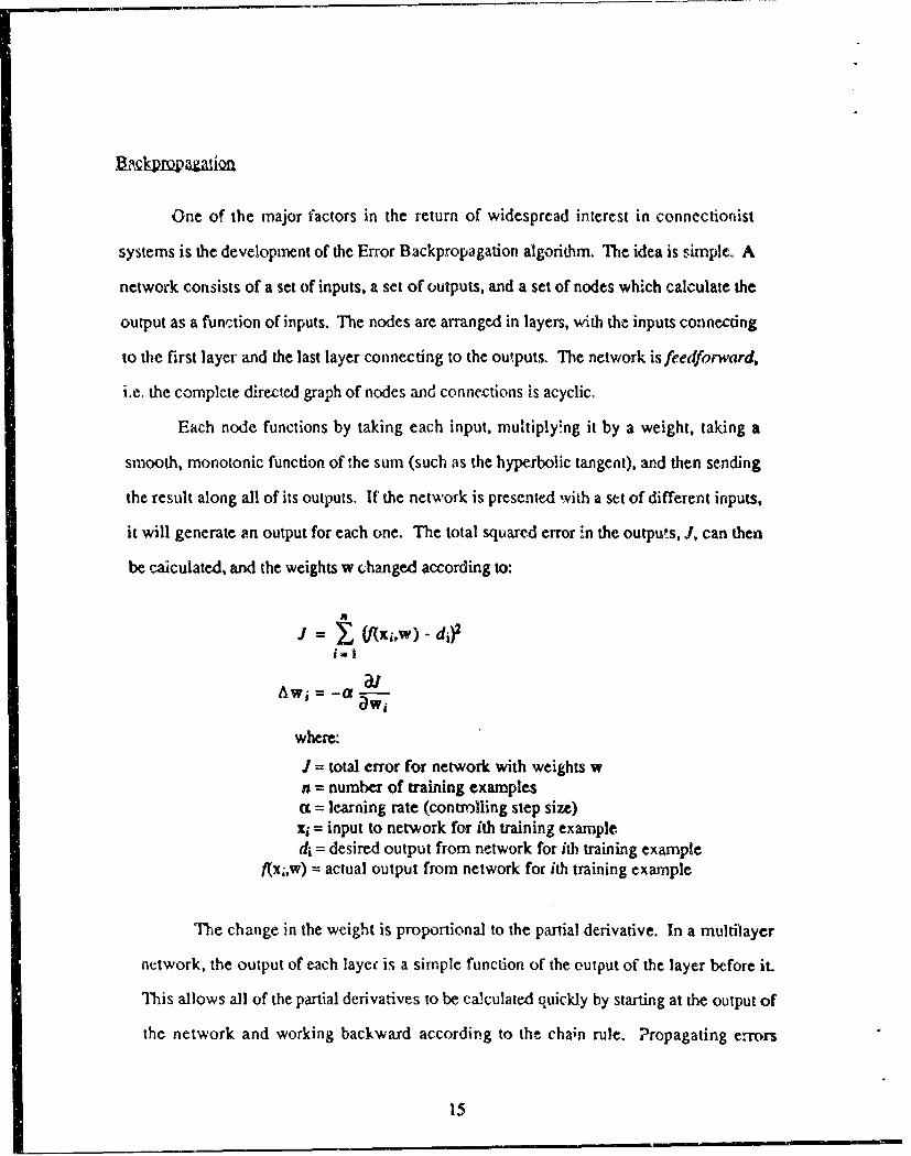
One of the major factors in the return of widespread interest in connectionist

systems is the development of the Error Backpropagation algorithm. The idea is simple. A

network consists of a set of inputs, a set of outputs, and a set of nodes which calculate the

output as a function of inputs. The nodes are arranged in layers, with the inputs connecting

to the first layer and the last layer connecting to the outputs. The network isfeedforward,

i.e. the complete directed graph of nodes and connections is acyclic.

Each node functions by taking each input, multiplying it by a weight, taking a

smooth, monotonic function of the sum (such as the hyperbolic tangent), and then sending

the result along all of its outputs. If the network is presented with a set of different inputs,

it will generate an output for each one. The total squared error in the outpu's, J, can then

be calculated, and the weights w changed according to:

J = i Vfxi,w) - di?i I

wi.)

where:

J = total error for network with weights wn = number of training examplesS= learning rate (contrnling step size)xi = input to network for ith training exampledi= desired output from network for ith training example

f(xi,w) = actual output from network for ith training example

The change in the weight is proportional to the partial derivative. In a multilayer

network, the output of each laye( is a simple function of the output of the layer before i.

This allows all of the partial derivatives to be calculated quickly by starting at the output of

the network and working backward according to the cha;n rule. Propagating errors

15

backward requires as little computation as propagating the original signals forward.

Furthermore, the error calculations can all be done locally, in the sense that information

need only flow back through the network along the connections between nodes which

already exist. These properties combine to make Backpropagation powertul yet low in

both computation time and hardware required.

This gradient descent process is simple and works well for multlayer networks, but

it is not guaranteed to find the best weights possible. As with all hiji climbing methods, it

can get stuck in a local minimum. Although this method cannot be guaranteed to find the

correct answer (as simple percepuions were), it is still a useful method which has been

shown :o work well on a variety of problems. Unfortunately, pure gradient descent

methods often converge slowly in the presence of troughs. If the error as a function of

network weights is thought of as a high dimensional surface, then a long, thin trough in

this surface slows convergence. If the current set of weights is a point on the side of a

trough, then the gradient will point mainly down the side cf the trough, and only slightly in

the direction along the trough toward the local minimum. If the weight chaages in large

steps, it will oscillate across the trough. If it changes in small steps, then it converges to

the local minimum very slowly.

There are a number of approaches to speeding up convergence in this case. One is

to look at the second derivative in addition to the gradient at each point. If a network has

one output and multiple weights, then the second derivative is a matrix giving the second

partial derivative of the output with respect to each possible pairs of weights. This matrix,

called the Hessian, has a useful geometric interpretation. Multiplying a vector by this

matrix stretches the vector in some directions and compresses it in others. For the direction

in which the error surface has least curvature, the Hessian will compress vectors. For the

direction in which the error surface has greatest curvature, the Hessian will stretch vectors.

Multiplying a vector by the inverse of the Hessian has the opposite effect. Multiplying the

gradient by the inverse of the Hessian will then cause the weights to change more in the

16

d tcfion along a trough (where the curvature is small), and less across a trough (where. the

curvature is large). If the network has N weights, this retiuires inverting an N by N matrix

on every iteration during training. This overwhelming flood of calculations may defeat the

purpose by requiring more computation than is saved by the shorter path to convergence.

This is why a number of approaches have been proposed for solving this problem, such as

using only the diagonal of this matrix, or using heuristics which approximate the effect of

the inverse Hessian.

2.2 TRADITIONAL CONTROL

Control theory deals with the problem of forcing some system, called the plant, to

behave in desired manner. The relevant properties of the plant which change through time

are calied the stare, and are iepresented by the real vector x. For example, in a cruise

control for a car, the state might include the current speed and slope of ground. If the state

cannot be measured directly, then the sensor readings are represented by another real

vector, y. The control action is the set of signals applied to the plant by the contloller, and

is represented by the real vector, u. The plant state then evolves in time according to:

it = f(x,,u,)Y1 = g(X1)

The maajority of control theory is devoted to the special case where the plant is

linear, in which case the state evolves according to

it = Ax,+Bu,

Y1 = Cxt

where A, B, and C are constant matrices. Even if a plant is not truly linear, it is often

close enough to linear within certain regions of the state-space that a controller can be

designed for that region based on a linear approximation of the plant. This is useful since

the theory for linear plants is better developed than for nonlinear plants [D'A88].

17

Once the plant has been modelled, the controller must be designed to accomplish

some purpose. If the goal is to keep the state at a certain value, then the controller is called

a regulator, If the go,' is to force the plant to follow a given trajectory, then the controller

is a model reference controller. If the goal is to minimtize some funciion of the whole

trajwetory, then it is an optinal control problem.

Traditional control techniques are based on approaches such as bang-bang,

proportional, PID, gain scheduling and adaptive control, each described in a section below.

These are important control approaches with which connectionist control techniques should

be compared. In addition to this, most of them are included, directly or indirectly, in the

hybrid system developed in this thesis.

Several of the systems described here were first demonstrated on a standard cart-

pole system. This plant is illustrated in figure 2.2.

D...W MW !MM

Figure 2.2 Cart-pole plant

The cart is confined to a one dimensional track, and force can be applied to it in

either direction to cause it to move left and right. On top of the cart is a pole, which is

hinged at the bottom and can swing freely. No forces are applied to the pole directly, so it

is only influenced indirectly through forces applied to the cart. The problem of balancing

the pole is similar to the problem of balancing a broomstick on a per son's haxid. This is a

standard control problem and is useful for demona;trating new control nethodxs, a version

18

of this problem is used here to test the new control systems developed in this thesis.

2.2.1 Bang-Bang Control

The simplest form of control is a controller which only has two possible outputs.

This "bang-bang" control is commonly used in thermostats which alternate between

running the heating system full on and turning it off completely. This type of control has

also been used in a learning system to balance a pole on a cart while keeping the cart within

a certain region [BSA831. Uniortunately, bang-bang control systems can't exercise very

fine control, and so lead to limit cycles in the plant being controlled, i.e. the state repeatedly

follows a certain path instead of settling down to a single state. A pole can actually be

balanced on a cart by always applying a certain force in the same direction the pole is

leaning, Naturally, this leads to the limit cycle of the pole swinging back and forth between

two extremes. Foi finer control, a more general controller is required, such as a

proportional controller.

2.2.2 Proportional Control

A proportional controller is perhaps the simplest controller imaginable that still has

continuously varying control actions. Each input to the controller is a real value,

representing one element of the state of the plant being controlled. In a regulator, that is the

only input, and the controller tries to control the plant so that all of the elements of the state

vector are zero. In a general controller, each element of the desired state vector is also an

input. The controller then multiplies each input by a constant gain, possibly adds a

constant, and uses the result as the control signal. If the control action is a vector involving

several signals, then the same process is followed for each of them, using a different set of

gains each time.

In order to design a good proportional controller, it is first necessary to have a good

model of the system being controlled. If the plant is linear and perfectly modeled, or even

19

if the plant is only close to linear, then it is often possible for a proportional controller to do

an acceptable job of controlling it.

2.2.3 P1D Control

If the control signal to a plant is simply proportional to the error in its state, then as

the state approaches the desired state, the correcting force will decrease proportionally.

Often, there will be some point near the desired point at which the small correcting force is

balanced by other forces, and the plant will settle into a steady state w" -h has a slight

error. In order to overcome this steady state error, the controller might integrate the error

over a long period of time, and add a component to the control signal proportional to this

integral. It may also be possible to improve the control signal by taking into account not

only the state, but also how the state is changing. For this reason it may be useful to add a

term to the control signal proportional to the derivative of the state.

If both of these modifications are made to a proportional controller, it is then called

a proportional plus integral plus derivative (PID) controller. If the input to this controller

and the output from it are considered as functions of time and the Laplace transform of

them is taken, then the relationship between input and output is simple. It is some

quadratic function of s divided by s. Li discrete time control, this means that the output of

the controller is a linear combination of four things: the output on the previous time step,

the current inputs, the inputs on the previous time step, and the inputs on the time step

before last. Since the output is at least partially proportional to the output on the previous

time step, small trrors in state 'an cause the output to keep incieasing until they are gone.

This is the integral portion of the controller. Since inputs from three different ti me steps are

used, it is possible to subtract them and estimate how fast the inputs are changing. This is

the derivative aspect of the controller. Also, since the curreat inputs affect the output

directly, it has a proportional control component. Therefore all three types of control are

present, and the controller is referred to as PID.

20

PID control is vcry widely used; in fact perhaps 90% of all of the controllers in

existence are PID controllers (or PI or P. which are just PID with some gains zero)

[PaI83]. If a plant is linear, it is often possible to design PID controllers that give the

desired performance. If a plant is nonlinear, but will usually stay in one small region of

state-space, then it is often practical to approximate the plant with a linear model in that

region and design a PID controller for that model. This n'iodei can be derived from the full,

nonlinear equations describing a plant, by taking the derivative of those equations, and

evaluati-ig it at a given point in the middle of the region of interest.

2.2.4 Adaptive Control

Instead of creating a fixed controller based on a priori knowledge of a plant, it is

sottimes beneficial to bWild a controller which can change if the plant is different than the

model, or if the plant changes or experiences disturbances. Starting in the early 1950's,

researchers enthusiastically pursued adaptive control, especially for aircr,'t, but without

much underlying theory. Interest then diminished in the early 1960's due to a lack of

theory and a disaster in a flight test [Asz831. More recently, adaptive control is finally

beginning to emerge as a widely used approach.

Adaptive control can be categorized as either indirect adaptive control or direct

adaptive control. Indirect adaptive control utilizes an explicit model of the plant, which is

updated periodically, to synthesize new contrel laws. This approach has the important

advantage that powerful design methods (including optimal control techniques) may be

used on-line; however, it has the key disadvantge that on-line model identification is

required. Alternatively, direct adaptive control does not rely upon an explicit p4ant model,

and thus avoids the need to perform mcdel identification. Instead, the control law is

adjusted directly, based on the observed behavior of the plant. In either case, the cor 'a'oller

will adapt if the plahn dynarrics change by a significant legree.

Adaptive controllers are usually designed with 1he assumption that the plant being

21

controlled may be poorly modelled, but is at least known to be linear, The controller itself

is also limited :o being linear at any point in time, but the "constants" in the controller

change slowly over time as it adapts. Even with all of these assumptions of linearity, the

entire system consisting of both an adaptive controller and a plant is not linear while the

parameters are adapting. This has made it very difficult to pruve that these controllers art

stable, although recent progress has been made in this area lAst83].

Adaptive control systems generally exhibit some delay while they are adjusting,

particularly when noisy senso-s are used (since filtering creates additional delay). If the

characteristics of the plant vary considerably over its operating envelope (e.g., due to

nonlinearity), the controller designed for a linear plant can end up spending a large

percentage of its time in a "partially" adapted state, leading to degraded perfomance.The

control system has to readapt every time a new regime of the operating envelope is entered.

2.2.5 Gain Scheduled Cont)l

A very nonlinear system could be controlledi by an adaptive controller which adjusts

to the new dynamics in each region of the state-space. Instead, most modeni control

systems handle nonlinearities with gain scheduled controllers. These controllers are

collections of simple proportional controllers, one for each region of state-space. For

example, in a typical complex control system, the state vector rnig•t include 30 elements,

three of which are special. When these three are kept constant, a simple, linear control law

can work well. The commands sent to die actuators can be a dt product of the state vector

and a gain vector. Wben any of the threr special elements change though, a new linear

conrol law with new gains must be used. In r gain scheduled controller, the space of al

possible values for those three state vector elements is divided up into ,yerhaps 300 regions.

Each region then uses a different set of gains, and a scheduler is tsed to stiloothly

transition whenever the state moves from one region to Pnother. The drawback to this

approach is that it requires a good mode! of the plant, as well as large anounts of heuristic,

22

hand tuned, calculations in order to guess where the boundaries between regions should

be, and what the control law in each region is. Once the controller is built, it cannot change

to accommodate a slowly changing plant, such as a robot where bearings wear and par.s

age. This control technique does respond instantly, though, when it enters a new region,

while the adaptive controller would have to wait for more intormation before it could adapt

to a new region, so gain scheduled control is generally used instead of adaptive control in

most complex systems today.

2.3 COINNECTIONIST LEARNING CONTROL APPROACHES

A number of different approaches have been suggested for using connectionist

sys, ems in control (Fu86][Bar89]. These systems generally try to solve one of three

control problems: producing given control signals, following given trajectories, or

optimizing given reinforcement or cost signals. For each of these problems there are one or

more different approaches which have been tried, the most common of which are described

beWow.

23

2.3.1 Producing given control signals

StateCommanded Control State

Controller PlantState +el•

N or,

Figure 2.3

The simplest use of a connectionist network in a control application is to emulate an

existing controuer. This is shown in figure 2.3. The controler and the network are both

told the current state and the state commanded (the state to which the controller should drive

the plant). The controller then calculates an appropriate control signd by some means, and

the network also calculates a control signal. If they differ, the difference is the error in the

network's output and is then used to train the network (shown by the diagonal line thr',mgh

the network). In the figure shown, the network has no effect on the behavior of the

system, it is simply a passive observer. Once the network has learned, the weights in the

network would be frozen, and the controller would be completely removed from zhe

diagram and replaced by the network. One early network, Widrow's ADALINE in the

1960's, was trained to balance a pole on a cart by watching a human do it, and learning

from that example [Wid89]. Almost any general supervised learning or function

24

approximation system can be used to control a system in this manner, although the

technique is obviously limited to systems where a control system already exists. This

appro. ¶. might actually be useful in situations where it would be too expensive or too

dangerous to have a human controllinig a system, but where a network could be used fairly

cheaply. It would also beo useful if it could be trained by example how to control in certain

states, and then could generalize to other states. These are unlikely to be very common

uses of such a system.

A more widely applicable use may be as a component of a larger control system

which learns to repr,"duce the results of the other components. For example, a control

algorithm may require an extensive tree search on each time step which takes too long to

implement in real-time, even in hardware. If it is possible to train a network to implement

the sarre mapping from state to outputs, then the network could replace the slow controller.

2.3.2 Following given trajectories

A much more corarnon control problem is that of following known trajectories. If

the plan- being controlled is fairly well understood, and if it .s not very nonlinear, then it is

often possible to specify a trajectory for the plant which is known to he both useful and

achievable. For example, if a robot arm is told to move from its curent position to a new

position, the ideal behavior might be for it to instanmaneously move to that position, and

comrrpletely stop moving as soon as it reaches it. This, unfortunately, requires the

application of infinite force to the arm. On the other hand, it requb-es very little force to

move the arm to the new position quickly but with a large amount of overshoot and

oscillation once it gets there, or to move it to the position slowly but with little overshoot.

There is a twade-off between force applied, time to get to the correct position, and time to

,settle once it is there. The exact niature of the trade-off depends on the particulat equations

governing the arm. Often, through partial models of the plant, trial and error, and

experience with similar plants, it is possible for a control engin4:,ýr to choose a particular

25

trajectory for the ann which is achievable and which gives acceptable behavior for the

pardcular application.

Choosing the reference trajectory may or may not be difficult in a given situation,

but it is extremely imiportant. If the reference trajectory is less demanding than necessary

(causing the state to approach the desired state very slowly and allowing a large amount of

overshoot), then the system will not perform as well as it could with a better controller. If

the reference trajectory is too demanding (causing the state to approach the desired state

rapidly with little overshoot), then the controller will attempt to use control actions outside

the range of what is possible, and the system may become unstable.

Once such a reference trajectory has been found, then the controller must simply act

at each point in time so as to m, ve the plant along that reference trajectory. Three

approaches foi" using connectionist systems in "model reference" control problems have

been explored: learning a plant inverse, dynamic Aigrs, and Backpropagation through a

learned model

Lzarning a plant inverse

State

iurren Plant2n4rse

2N ork Next

Control +f[•v '•.4•' ILontroI

Figure 2.4

26

StateCommandedTrained Plant Control State

• _ . __ InversePan

State Network

I Desired Next State

L ~ReferenceI

Figure 2.5

A conceptually simple approach to model reference control is to use a network to

learn a plant inverse. In a deterministic plant, the state of the plant on a given time step is a

function of both the state and control action on the previous time step. Alternatively, in

continuous time, the rate of change of state at a given point in time is a function of the state

and control action at that point in time. An inverse of this function with respect to the

control signal is a useful function to know. Given the current state and the desired next

state (or desired rate of change of state), an inverse gives the conutol action required. If a

network can learn such an inverse then it can calculate the control actions on each time step

which will cause the plant to follow a desired trajectory.

Figure 2.4 illustrates how a network is trained to learn the plant inverse. FWst,

some kind of exploring controller is used to drive the plant. This may not be a very good

controller, in fact it could even behave randomly. Its purpose is simply to exercise the plant

and show examples of various actions being performed in various states. The network

then takes two inputs: the plant's state at the current time and the plant's state on the

previous time step. The output of the network is then its estimate of the control action

which caused the plant to make the transition from one state to the other. This estimate is

then compared to the actual command to generate the error signal used to train the network.

21

Figure 2.5 shows how the network is used after it has learned. Given the current

state of the plant and the desired next stawe (as specified by the reference trajectory), the

network generates a control action to move the plant to that new state. If the next state of

the plant does not match the desired state perfectly, then this error could be used to continue

training the network. In this way, the network could learn to control a plant whose

dynamics gradually change over a long period of time.

A fundamental problem with learning the inverse of the plant is the network's

behavior when the plant does not have a unique inverse. Most network architectures, when

trained to give two different outputs for the same input, will respond by learning to give an

output which is the average of the training values. For example, if a plant at a particular

state can be forced to act in the desired way by giving a control signal of either I or 3, the

network will usually learn an output of 2 for that state, which may be a far worse action

than either 1 or 3.

If the plant is a stochastic system, then the result of a single action will be an entire

probability distribution function, which further complicates the problem of learning elther

the forward or inverse model, and of choosing the best action. These problems often limit

the usefulness of learning plant inverses.

28

StateCommanded

Hr.ler Contol State

S tate kN_

P lant

Multiply byDynamic Signs

ReferenceDesired Next State +

Figure 2.6

A learning zystem using dynamic signs is shown in figure 2.6. For a given state,

the network tries to find an action which will drive the plant to the next state on the

trajectory defined by the reference. If it does this, then the new state will equal the output

of the reference, and tht subtraction will yield zero error, so no learning will occur. On the

other hand, if there is an error in the state, then each weight in the network should be

adjusted proportionally to its effect on that error. Finding the effect of a given weight on

the control signal is easy; it is simply the partial derivative of the control with respect to that

weighL In order to find its effect on the plant's state, however, it is necessary to know the

partial dtrivative of the state of the plant with respect to the control signal.

Often the general behavior of a plant is known, even though all the exact equations

and constants are [iot known. For example, it is often clear that applying more control

action will cause one element of the state to increase and another one to decrease, even

though it is not possible to piedict exactly how much change will occur. In this case, the

partial derivative of state with respect te control is no. known, but the sign of the partial

derivative is known. If the actual partial derivatives were known, then the error in state

29

would be multiplied by the derivative before being used to train the network. Since only

the sign of the derivative is assumed known, each element of the error is merely multiplied

by plvs or minus one. Figure 2.6 shows how the error in the state is multiplied by this

value before being used to train the network. This "dynamic sign" has been shown in

some cases to contair enough information to cause the network to converge on a reasonable

controller [FGG90. It has been shown ¶GF90I[BF90 that for autonomous submarine

control with a mu'tiddnensional state vector and a scalar control, the system can learn to be

an effective contjlle" using dynamic sign,.,.

State 4%Commanded -__

C~ m~ ~ dC C on . e 1Control !State

s t eo -L k P l. .tNetworkState_ ___

+

Reference

___ __ __Desired Next State+

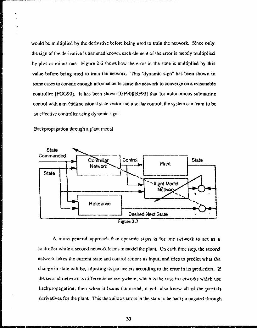
Figure 2.7

A more general approach than dynamic signs is for one network to act as a

controller while a second network learns to model the plant. On tach time step, the second

network takes the current state and coniio!. actons as input, and tries to predict what the

change in state wili be, adjusting its parrnieters according to tht. error in its prediction. If

the second network is 6ifferentiabie ev:rywhere, which is the case in networks which use

backpropagation, then when it learns the model, it will also know all of the parti;4s

d(rivatives for the plant. This then ailows errors in the state to be backpropagate-1 through

30

both networks in order to change the parameters of the first network so that it can learn to

control the plant model. This is the same as the dynamic signs approach described above,

except that the par-tial derivatives across the plant are estimated automatically instead of

being set to plus or minus one by hand according to a priori information.

Figure 2.7 illustrates this process. The network on the right is trained to predict

what the next state of the plant will be, given the current state and control. This training is

indicated by the solid diagonal arrow through the network. At the same time, the network

on the left is trained to be a better controller. This is done by propagating the error in state

through both networks, while only changing weights in the controller network. Although

this signal propagates through the plant model network, it is not used to traip that network,

which is why it is represented in the diagram by a dotted arrow. This approach has been

successfully used by Jordan [Jor 883.

2.3.3 Optimizing given signals

The above techniques are all based on the assumption that there is a reference

trajectory to follow. At each time step, given the current state, it is assumed that the desired

change in state is known. For some systems though, finding a reference trajectory is fully

as difficult as finding the controller in the first place. For example, a large semi truck

consists of two sections with a hinge between them. If the truck is near a loading dock and

at an zngle to it, it can be difficult to calk.ulate how to back up the truck so that it ends up

with the back end lined up with the dock [NW891. This procedure may involve tunning the

wheel all the way to the left, backing up some, then gradually turning it to the right, then

finally straightening it out, causing the truck to follow an S shaped path. If the path to

follow is known, it is trivial to calculate how to turn the wheel to follow the path, but

finding the correct path in the first place is a difficult problerm. The model reference

systems discussed above are therefore not useful for solving this type of problem. In thin

case, the goal is actually to minimize a quantity after 1 certain period of time (the distance

31

m m • m m m u m :, in m 'm m n n m z•'m n • ,| nw u

from the dock at the end), rather than to follow a given u-ajxctory.

This is just one example of the most general type of control problem, which is tie

optimization of some quantity over time. This is called PReinforcement Learning" since the

goal of the controller is to maximize some external reinforcement signal over time CWil88].

Since several actions may be performed before the reinforcement is received, it is often

difficult to determine which of the actions were good and which were bad. This "temporal

credit assignment problem" makes reinforcement learning the most difficult type of problem

considered here. Control problems of this type include backing up a truck to minunize the

error at the end, finding the route to the moon which requires the least fuel, or finding the

actions for an animal which maximize the amount of food it finds. All of these cases

involve maximizing a reinforcement (or n,. -nizing a cost) over some period of dime (finite

or infinite). This is a difficult problem, since it may be necessary to do actions which arm

worse in the short run, but art better in the long run. If a controller generates some action

and then receives negatve reinforcement (or positive cost), it is not clear whether that is

immediate result of that action or the delayed result of a much earlier action. Thus it is not

clear how to leanr the correct action, or even how to evaluate a given action.

This difficult control problem has been addressed by Backpropagation through

time, actor-cr:ic systems, and dynamic programming systems. Actor-critic systems and

dynamic programrnming systems tend to be, broad categories with some overlap, but are a

useful way of classifyng the many approaches to this type of problem.

.,2

ckprolpagatio rough in

StateCommanded Exploring ControlState

- ControllerState

PI Model

Figure 2.8

One way to solve this problem is to extend the idea of backpropagating through a

plant model. Two networks are used. One is trained every time step to learn to model the

plant. Figure 2.8 shows how the network can learn to model the plant using the current

state, the previous state, and the previous control action.

StateCommanded ,._I Controller Control Plant Model State

;L Network NetorState ... . ' ' " Newr

Figure 2.9

33

Once it has learned, the other network can learn to be a controUer based on the plant

model. The two networks are connected as shown in figure 2.9. With all parameters

fixed, the plant model starts at some initial position, and the controller network controls it

for a period of time which is known to be long enough to get the plant into the correct

position (alternatively, it controls it unti: it tries to leave the boundaries of the area which

the plant must stay within, or it simply controls it for a long period of time). All of the

signals going through the networks are recorded during this trial.

Initial state State commanded State commandedcommanded at time 1 at time N

Cton~tvlek- -0 Modei4e Contibo8 1s ModeiNe C4toe Model*

Initial State State at State attime 1 time N

Figure 2.10

The two networks are then unrolled in time, so that it looks like the signals have

passed through a very long network once, instead of passing through two small networks

many times. The cost or reinforcement signals are calculated from the plant model state at

certain time steps of the unrolled network. In the case of the truck backer-upper [NW89],

this signal is zero on every time step until the end, and then is equal to the error in state

after the last time step. This error can be backpropagated through the large network to

change all of the parameters, thus changing the controller t. be slightly better throughout

the whole trial. This "backpropagation through time" has been shown to be able to solve

the problem of backing up a truck [NW89]. It is related to ideas suggested by W'rbos

34

[Wer89] and work done by Jordan [Jor881 and Jameson [Jam90] where signals are

propagated back through time during training.

Backpropagation through time does have the difficulty unfortunately, of requiring

that every signal on every time step for one trial be saved. For long trials this could be a

problem. Other algorithms could be used instead, such as the Williams Zipser algorithm

for training recurrent networks [WZ89]. This has memory and processing require ,ents

independent of the length of the trial, but proportional .o the cube of the number of nodes

(assuming fi'"y interconnected nodes), so it can also be impractical fou large networks.

Actor-critics

Backpropagation tluough time is a potentially very useful technique, but is still not

completely general. Even assuming the ietworks can perfectly m,"del the functions they

are trained with, the result will still be a controller which causes the plant to follow a locally

optimal path. The path will be such that a ay small change to it will make it worse, but a

large change to the path as a whole could still improve it significantly. The

backpiopagation through time algorithm also requires storing all of the signals going

dtrough the network throughout the whole trial. In a regulator problem, where the the plant

may never fail and may never reach the goal state exactly, the trial will be infinitely long.

An alternative approach that avoids some of these difficulties is to use a system with two

components, called an "actor" and a "critic". The actor is the actual controller which, given

the state, decides which control actions should be used. The critic is a component which

receives external reinforcement signals and uses them to train the a,;tor. This is a difficult

problem, since reinforcement may come long after the actions which caused it. In fact, the

beist actions may actually increase errors be 1ore they start to decrease them, and the c-itic

must mrcogni-e that this is the case. For example, for the c-trt balancing a pole, if the cart

starts at the origin with the pole balanced, and the goal is to move one meter to the right, the

reinforcement on each time step might be the negative of the position error. The fastest

35

way to move the systemr one meter to the right without allow'ng the pole to fall over, is to

first move ieft, causing iMe ole to dih io the right, then move qui,:kly to the right. Thus the

error in position should increase 'x fore il. decreasec. If the actor is to learn tile control

actions which will ar;:omplish this, the, critic must fa;st learn to recognize that this is

desirable. It will have to learn that a large po~sition ercor with the pole tilted the right way is

preferable to a smaller position error with e pole t 'ted the wrong Wa>'.

Samuel's checker player 'Sam591 was one of wne eva-liMt systems to take this

appr3ach. The actor was an algorithm which switc' A between book playing and an ajija.

beti. t~ee seai ,h. The search was based on the relative desirability of various board

positions, as decided by the critic. The critic was a linear combination of several hand-built

heuristic functions, and learning for the critic consisted of adjusting the weights of the

linear combination, and also deciding which of a large number of heuristic functions should

be included in the combination.

Michie ana Chambers [MC68] developed the Boxes system which consisted of ar,

actor and a simple critic They applied their controlier to a cart pole system which would

signal a failure whenever the pole fell over. The critic based its evaluation of a state on the

number of time step3 betwxeen entering that state and failure.. This system was later

improved by Barto, Sutton, and Anderson [BSA83) with the development of the

Associative Search Element (ASE) a Adaptive Critic Element (ACE). In that system, the

critic based its evaluation on boh the time until failure and ,.he change in evaluation over

time. Evaluations were therefore predicting both the desirability of a given state, and an

estimate of what the evaluations would be. in future states. This system learn-A to balance a

pole on a cart more quickly than the Boxes system.

Dynwimic PrngranLing_5_ym

Dynamic programming is a class of mathematical techniques for solving

optimization problems. Often the sets of possible states and actions are finite. The

36

problem is to find the best control action in each state, taking into account that it may be

profitable to perform actions with low reinforcement (or high cost) in one state in order to

reach another state which gives high reinforcement (or low cost). Not only is a suggested

action learned for each state, but typically one or more other values are associated with it as

well.

The most common formulation of dynamic programming associates two values

with each state. A "policy" is the action which is currently considered to be the best for a

given state. An "evaluation" ,If a state is an estimate of the long term reinforcement or cost

which will be experieniced if optimal actions are performed, starting in that state. All of the

policies and evaluaficns are initia'lized to some set of values, and then individual values are

improved in some order. A given policy or evaluation is improved by setting it equal to the

value which would be appropriate for it if the values of its neighbors were correct. If this

process is done repeatedly to policies and evaluations in all the regions, then under certain

circumstances it is guaranteed to converge to the optimal solution [WB90]. The set of

policies function somewhat as an actor, while the se. of evaluations function as a critic.

Reinforcement learning with actor-cr~tic systems may therefore sometimes be thought of as

a kind of dynamic programming.

Other types of dynamic programming systems do riot resemble actor-critic systems.

Q learning, devised by Watkins ,Wat89], only involves one type of value. For each

possikble action in each possible stace, a number (the "Q value") is stored which represents

the expected long term results if that action is performed in that state followed by optimal

actions thereafter. As in the other forms of dynamic programming, a Q value is updated by

changing it to be c, oser to the value that would be appropriate for it if the Q values of all its

neighbors were assmied to be correct. Q learning is also guaranteed tnder certain

assumptions to converge to the optimal answer.

The above discussion assumed that the sets of possible states ane actions were

finite. If there is a continuum of states and actions, then an approximation to dynanih

37

programming must be used. The most common approximation is to divide the state.space

into small regions, and store evaluation and policy values for each region. If the state-

space is very high dimensional, this will require prohibitively many values to be stored,

and dynamic programming will not useful. A natural solution to this "curse of

dimensionality" is to use some form of function approximation system to store the

evaluation and policy for the entire continuum of states. Connectionist systems would be a

natural candidate for this use.

This section has described systems for solving the problems of emulating a given

controller, following a given trajectory, and optimizing a given signal. None of the

systems described here make use of much a priori knowledge of the plant. Often fairly

good models of a plant may exist, and it would be useful to have some method for quickly

integrating this knowledge into the controller. The systems described here also tend to

react very slowly to changes in the plant, since the network must leamn a new function

whenever the plant changes. These are the problems which this thesis addresses.

38

3 HYBRID CONTROL ARCHITECTURE

The architecture presented here represents a new methr ,of integrating leaning and

adaptation in a synergistic arrangement, forming a single hybrid control system. The

adaptive portion of the controller provides real-time adaptation to time-varying dynamics

and disturbances, as well as any unknown dynamics. The learning portion deals with static

or very slowly changing spatial dependencies. The latter includes any aspect of the plant

dynamics that varies predictably with the current state of the plant and the control action

applied.

A conventional adaptive control system reacts to discrepancies between the desired

and observed behaviors of the plant to achieve a desired closed-loop system performance.

These discrepancies may arise from time-varying dynamics, disturbances, sensor noise, or

unnmodeled dynamics. The problem of sensor noise is usually addressed with filters, while

adaptive control is used to handle the remaining sources of observed discrepancies. In

practice, little can be done in advance for time-va.:ying dynamics and disturbances; the

control system must simply wait for these to occur and then react. On the other hand,

unmodeled dyniamics that are purely functions of state can be predicted from previous

experience. This is the task given the learning system. Initially, all unmodeled dynamics

are 'handled by the adaptive system; eventually, however, the learning system is able to

anticipate previously experienced unnmodeled dynamics'. Thus, the adaptive system is free

to react to time-.varying dynamics and disturbances, and is not burdene,] with the task of

rezctiog to predictable, unmodeled dynamics.

The hybrid adaptive / learning system accommodates both temporal and spatial

lThis a.ssumes, of ourse, that tie order of Ow. plant (dimension of its state vectot) is accwatky known.

39

modeling uncertainties. The adaptive part has a temporal emphasis; its objective is to

maintain the desired closed-loop behavior in the face of disturbances and dynamics that are

time-varying or appear to be time-varying (e.g., a change in behavior due to a change in

operating conditions). The learning part has a spatial emphasis; its objective is to facilitate

the development of the desired closed-loop behavior in the presence of unmodeled

nonlinearities in the state-space. Typically, the adaptive part has relatively fast dynamics,

while the learning part has relatively slow dynamics. The hybrid approach allows each

mechanism to focus on the part of the overall control problem for which it is best suited, as

summarized in Table 3.1.

--- Adaptation Learningtive: constructional:naintain desired ynthesize desired

losed-loop behavior losed-loop behaviormporal emphasis patial emphasis

no memory =*, mmory =*anticipation ticipation

ast y-namics low dynamicsocal optimization lobal optimization

-time adptation esign& on-linctime-varying ningynamics) spatial nonlinearities)

Table 3.1 Adaptation vs. learning.

A schematic of one possible realization of a hybrid adaptive I learning control

system is shown in Figure 3.1.

40

INDIRECT CONTROLADAPTIVE o PLANT

CONTROL SYSTEM_

ANTOIPATF.D POSTERI1OR _

BEHAVIOR ESTIMATEOUTPUT ISTATE

SYSE

Figure 3.1 Hybrid adaptive /learning controller.

To simplify the discussion, we assume that all necessary plant state variables are

observable and measured; in the event that this is not the case, a state observer would have

to be used. The indirect adaptive controller outputs a control action based upon the current

state, the desired state, and the estimated model of the system being controlled. This

estimate characterizes the current dynamical behavior of the plant. If the behavior of the

plant changes, the estimator within dte adaptive controller will update the model. If plant

changes are unpredictable, then the estimator will attempt to update the model as quickly as

possible, based on the information available in the (possibly noisy) sensor readings.

Adapting to predictable model errors that are functions of state will take just as long as

adapting to unpredictable disturbances and temporal changes, assuming similar noise

levels.

This problem is handled by the learning system in the outer loop. It monitors the

indirect adaptive controller's posterior estimate of the plant parameters, and learns to

associate each point in the state-space with the appropriate plant parameters at that point.

The learning system can then anticipate plant behavior based on past experience, and give

its prediction to the indirect adaptive controller. This allows the controller to anticipate

41

predictable dynamics while still adapting to unpredictable dynamics.

The learning system used here is a feedforward multilayer network. The input is

the current state, and the output is a prediction of what the plant parameters should be.

Prior to learning, the network is initialized so that the the hybrid controller will give the

same control signals that the adaptive controller would give by itself. When the network

has correctly learned the mapping, the hybrid adaptive / learning controller will anticipate

nonlinear model errors which are functions of state and are predictable, and will respond

faster than a simple adaptive controller would. If these structural nonlinearities change,

then the hybrid will act as an adaptive controller until it learns the new mapping. The entire

system is automatic; no explicit switching criterion is needed to go from adapting to

learning.

Any type of connectionist network can be used for the learning system, it need only

have the ability to learn functions from examples. This part of the system could even be

some other form of Pssociative memory such as a lookup table or a nearest neighbor

classifier. In practice, though, these types of techniques may be impractical since a

potentially infinite number of example points are used for training, and the state-space may

have a very high number of dimensions. For this reason, a connectionist network seems

more appropriate.

3.1 THE LEARNING COMPONENT

The hybrid architecture allows any learning system to be used which can learn to

approximate a function from a large set of examples of that function. The first learning

system examined here was a fee dforward, Backpropagation, sigmnoid network. The inputs

to the network and the outputs from the network were scaled to vary over a range of unit

width. The training examples were stored in a large buffer, and were presented to the

network in a random order. The network. was trained incrementally; weights were

42

changed after each traiaiing example was presented.

"The network was then tried with Delta-Bar-Delta, a heuristic method which

approximates tht. effect of using the Hessian to scale the weight changes. A modified

version of Delta-Bar-Delta was then tried, comparing two traces with different time

constants.

The learning systems, and the reasons behind their choice for this application, are

desciibed in further detail in chapter 4.

3.2 THE ADAY.VE COMPONENT

The adaptive component of a hybrid controller can be any indirect adaptive

controller which can incorporate outside information. The controller might for example

estimate parameters of the plant, and then act as the best controller for those parameters. it

might instead estimate the amount of error in its predictions of state on the next step, and

try to compensate for it. For the experiments done here, an indirect adaptive controller

which estimates such errors was used, both in its original form and with modifications.

3.2. 1 Tune Delay Control

A system called the Time Delay Controller (TDC) was chosen as the adaptive

controller for the experiments presented here. TDC is an indirect adaptive controller

developed by Youcef-Tourmi and Osamu [YM90].

This system works by looking at the difference between the ,urrent state of the

plant and the state of the plant on the previous time-step. This difference, along with

knowledge of what action was chosen on the previcus tirne-step, is used to estimate the

effect that the unmodeled dynamics are having on the system. This value, H, is calculated

explicitly and plays a pivotal role in the next calculations. The control action is then

modified 'o cancel these unwanted effects and to insert the iesired dynamics into the plant.

43

Thie technique uses inforrnation that is only one time-step old, so it is able to react to

sudden changes in the plant or environment after a single time-step. Of course, since it is

in effect differentiating the state, it, is sensitive to high frequency noise. Youcef-Toumi

points out that this is not as bad as it sveems if the plant itself acts as a low-pass filter,

attenuating the effect of the noise in the control actions.

The corttroller can also be made less sensitive to very high frequency noise by

simply using a larger time-step and a filter. This, however causes it to react more slowly to

changes in the plant. Overall, TDC does a good job, but it cannot both react quickly and

remain insensitive to high frequency noise.

3.3 THE HYBRID SYSTEM

The connectionist network used in the hybrid adaptive / learning controller is a

simple, feedforward, back-propagation network, with two hidden layers of ten nodes each.

Given the state and goal for the plant, the network is trained to output the unmodeled

dynamics H. In the absence of noise, this should be the same H that TDC calculates. If

noise is present, it may be possible to determine the current state of the plant to within a

small error. The correct H, however, is difficult to calculate precisely, because it is found

by "differentiating" dte state (e.g. using a backwards difference).

One property of connectionist networks is useful here. During training a network is

given input and desired output values repeatedly. If it is given conflicting desired outputs

for the same input, then it tends to average them. This means that the network can be

trained with data that has small, zero mean noise and still learn the same function.

The;efore, if TDC calculates noisy H's with an equal probability of the value being too

high or too low for' a given state, and if thest are used to train the network, then the

network will tend to learn the correct H for each state.

The network is not only useful when H is noisy; it is also helpful when it "s used to

44

predict H. In this case, TDC looks at the state of the plant before and after a given time-

step. Back-differencing to estimate the derivative, TDC can now calculate the unmodeled

dynamics H during that period. That H is then used to calculatc the appropriate control

action to be applied to the plant during the next time-step. This is a source of error in the

controller, since it is always sending out control actions based on what was correct on the

pievious time pediod. With the network, there is a simple solution to this problem. Instead

of associating H with the current state during training, it is associated with the previous

state. After the network has been trained with those patterns, it should be able to predict,

given a state, what H will be during the time-step following that state. This allows a better

estimate to be calculated.

The hybrid controller, therefore, has at least the potential to solve both of the

difficulties with the original adaptive controller. This is in addition to the main problem it

was designed to solve- learning control. These considerations provide motivation for

experimenting with the hybrid controller.

The hybrid adaptive / learning controller typically runs at a speed somewhere

between 10 Hz and 50 Hz. At these rates, the states and H do not change much over a

period of several time-steps. If the network is trained on similar states several times in a

row, it may forget what it knows about other states. One solution might be to train the

network less frequently, such as once a second. This might be effective, but it would slow

down learning by not learning every thne-step. A better solution is to use a random buffer.

During training, as the plant wanders through the state-space, the data from each time-step

is stored in the buffer. One point is also chosen at random from the buffer on each time-

step, and is used to train te network. This ensures that the network is trained on a well

distributed set of points.

45

3.4 DERIVATION OF THE HYBRID W'TH KNOWN CONTROL EFFECT

The original TDC equations were designed to allow the incorporation of a priori

information consisting of a linear model of the plant. The effect of control action on state

was assumed to be known perfectly, but the other parameters could iiiitiakly be incorrect.

The following is a derivation of the TDC equations for a discrete time plant where the

known dynamics are given by the a priori knowledge 0 and F, as well as the knowledge

gained by the learning system, 'V. As in the original TDC, the effect of control on state is

assumed to be a linear function, and the constant F is assumed to be knowrn without any

error.

Assume that the plant being controlled is of the form

x(k+l) = !xwk) + um(k) + 'V(x(k)) + h(x(k)k) (1)

where at time k, x is the state vector, u is the control vector, all of the unknown dynamics

are represented by the function h.

The tference trajectot- has the dynamics

Xm(k+I) = (%'xm(k) + rMr(k) (2)

where :- is the command vector. The error between ,he actual state and the refereirce, state is

Q(k) = xm(k) - x(k) (3)

The g&at is to build a controller that will cause the error to behave as:

e(k+I) = ({•.+K}e(k) (4)

where K is the error feedback matrix. By using a nonzero K it is possible to make the

46

desired dynamics faster whenever the plant drifts off of the reference trajectory, thus

forcing it back to that trajectory. If K is zero, then the behavior will be the same except that

small errors in the state will accumulate over time.

Substituting (3) into the left side of (4), then substituting (2) into the result and

solving for x(k+l) gives th'e desired next state:

Xm(k+l) - x(k+l) = ({m+K)e(k)

0 'mxm(k) + Frar(k) - x(k+l) = (Om+K)e(k)

x(k+l) = O2ImXm(k) + Fmr(k) - •'Dm+K)e(k) (5)

Setting (1) and (5) equal and solving for u gives the control law which should be

followed in order to achieve the desired next state.

'Mx(k) + ru(k) + •F(x(k)) + h(x(k),k) = cmxm(k) + Fmr(k) - ({'m+K)e(k) (6)

u(k) = r1( 4'mXm(k) + rmr(k) - ({Dm+K)e(k) - Ox(k) - 'V(x(k)) - h(x(k),k) (7)

where, for a matrix M, M+ =- (MTM)-IM'T is the pseudo-inverse of M. The only unknown

in (7) is h. If h changes slowly, then it can be approximated by its previous value.

So~lving (1) for h and then applying this approximation yields:

h(x(k),k) = x(k+l) - Ox(k) - ru(k) - 'l(x(k)) (8)

h(x(k),k) x(k) - 4x(k-l) - Fu(k-i) - '(x(k-l)) (9)

Substituting the approximation (9) into equation (7) gives the final control law

u (k) = Fr-(mxn(k) + rmr(k)- ({m+K)e(k) - 4Dx(k) --* (x(k)) (10)

- x(k) + x x(k-1) + Fu(k-l) + T(x(k-1)))

The controller will adapt to a sudden change in the plant dynamics within I time

47

step. If the time step is short, the controller will respond faster, but will also be more

sensitive to noise.

3.5 DERIVATION OF TE RHYr fD WITH UNKNOWN CONTROL EFFECT

It is often the case that the exact effect of control on state is only partially known,

just as the dynamics of the state are only partially known. If a learning system can learn the

unmodeled dynamics, then the partial derivative of the learned function, T, with respect to

control action, u, will represent the unmodeled effect of control on state, and can be used

to improve the a priori estimate of this value, r. The following is a derivation of the hybrid

system, incorporating these partial derivatives as an improvement over the approach in

section 3.4.

Assume that a plant has the following dynamics:

x(k+l) = Ox(k) + 17u(k) + P(x(k), u(k)) + h(x(k),u(k),k) (11)

where the vector x(k) is the state at time k, the vector u is the control, the matrices 0?> and r

and the function T' are the known dynamics, and the function h is all of the unknowns,

including unmodeled dynamics, nonlinearities as a function of state or control action, and

time varying disturbances.

The reference trajectory has the dynamics

Xm(k+l) = bmxm(k) + Pmr(k) (12)

where r is the command vector giving the state to which the plant should be diiven. The

error between the actual state and the reference state is

e(k) = xm(k) - x(k) (13)

48

anid the goal is to build a controller which will cause the error to d&crease according to:

e(k+l) = ({m+K)e(k) (14)

Substituting (13) into the left side of (14), substituting (12) into the result of that,

and then solving for x(k+1) gives the desired state on the next time step.

x(k+1) = 4mxm(k) + Frr(k) - ({m+K )e(k) (15)

All known dynamics not defined by D and F are represented by the function P,

This can be learned or stored in any manner which allows the calcvjlation of the partial

derivatives with respect to u. When calculating the u for a given time step, it will be

necessary to take in to account the fact that T may affect the next state differently according

to which u is chosen. Figure 3.2 illustrates how T, ,ai' be approximated by evaluating it at

the current state and previous control action, then forming a line through that point with the

appropriate slcpe in the u direction. Equati-n (16) shows this approximation

mathematically.

49

T'(x(k),u(k)

'(x(k),u(k- 1)

U

'P(x(k-1),u(k-1)

Fig,-e 3.2 Approximation of IF as a function of u(k) for the current value -f x.

'T(x(k). a(k)) - 't(x(k), u(k-1)) + (u(k)-u(k-l)) (16)UL(k). u(k-l)

Substituting (16) into (II) gives a more useful formulation of the plant dynamics.

x(k+l) = (Dx(k) + Fu(k) + I'(x(k), u(k-1))

+ (u(k)--u(k-l)) + i,(k,x(k),u(k)) (17)(ak), u(k-1)+

If the function h representing disturbances etc. is changing slowly, then it can be

approximated by solving for h in (17) for the previous time step, and using thai as the

approximation of h for the current time step.

50

h(k,x(k),u(k)) -x(k) .- <x(k-1) - ru(k-1) - T(x(k-1). u(k-2)) (18)

- u~k-2)k , ), u(k-2)

Substituting (18) into (17) and solving for u(k) gives the control law, in terms of thedesired next state x(k+l).

u~)=(r+qau k),u(k-l)) ) I aIx(k), u(k-1) (9

-Dx (k) - T/(x (k), u (k- 1)) + x (k+ I

- x(k) + Ox(k-1) + ru(k-i) + T 5(x(k-1), u(k--2)1,

+ (U11-1) - u(k.-2)) ýTlk)uk-]

Substituting the desired next statt (IS) intO (19) yields the finxal control law:

u~k) ' =(+j,(k), u(k 1))[ au 6L(k), u (k-1) (0

-O k)-- 'V(x(k), u(k-1)) + Omxm(k) + " r(k) - [0,+K)e(k)

-x(k) + Oix(k--1) + ru(k-i) + IV~xk-l), u(k-2))

+(ti~k--I) - eji%-2)! ?,{( I)

51~-) uk2

4 LEARNING SYSTEMS USED

The le-uning component of the hybrid is responsible ior learning the function which

the adaptive controller discovers a posteriori. Because the, function is defitied over a

continuum of states, and can involve large numbers of dimensions, connectionist systems

were chosen for the learring component. First a standard Backpropagatiorn network was

used, as descnbed in the next section, then linear gaussian networks and Delta-Bar-Delta

learning were. added, as described in the following zwo sections, to increwae learning speed.

4.1 BACKPROPAGATION NETWORKS

During the operation of an indirect adaptive controller, certain parameters are

estimated on each time step, and the controller uses these to choose an appropriate control

action. Ether on the next time step, or soon thereafter, the controller may have additional

information about what the estimates should have been earlier. It is natural to consider

whether a learning system of some sort could learn to map the earlier state to later,

improved estimates, and so be able to make even better estimates the next time that state is

entered. This is simply a functior approximation problem.

The function being learned wold output parameters as a function of state. The

par-ameters and the state may be high dimensional vectors, and the function being learned

may be need to be generated on the basis of a large number of training points generated by

the indirect adaptive controller. In this case, a Backlropagation network would seem to be

a good model for learning the functions involved. For any given function and desired

accuracy, a network can tit found which will learn that function to the desired accuracy

[HW89]. This is true for networks built from any of a wide range of functions.

52+ ~ ~ ~ ~ ~ ~ ~ ~ ~ ~ ~ ~~1 KIM' ""•rru',,v !,'"!,, 'm, , !1 r ,me• •-

There are a number of considerations which arise wher trying to apply

Backpropagation networl's to learning functions in :Nhs context. First, the data used to train

the network comes from a controller controlling an actual plant. In this case, the training

data will consists of states and the appropriate paramieters which should be associated with

them. The state used for training will always be a recent state of the plant, and since the

state of a plant may not chan~ge much on each time step, the training data during a given

period of time will all tend to come from one region of the state-space. This is even more

applicable in the case of a regulator. In a regulator, the controller tries to keep the plant

near a certain state all tde time. If the controller is doing a good job and there are no large

disturbances, the state of the plarAt will stay near where it should be. This means that no

training points will be generated in other regions. Even in a model reference problem, the

plant may still move slowly thrcugh state-space. Therefore it is important to consider the

ability of a given learning system to learn despite repeated exposure to very similar training

pattems for long periods of time.

Bzickpropagafion, and most of its ,ariantc, all try to adjust the wei Ihts to follow

son;-e gradient and decrease trror, as decribed in chapter 2. The error being minimized, J,

is frequently defined as the mean squared error between the network output and the desired

value of its oatput, summed over all pxossible inputs:

afi

where:

J - Towal cror for network with weight vector wn = nurntbr of training exa_,mples

xi input to network for ith training exampledi= desired output of iietwork for ith training example

f(x,..w) actual output of network for ith training example

"ris implies that the network is be updated by epoch learning, where weights arc

53

mm

changed once per epoch (pass through all the training examples). However, for the

function approximation being done here, the function being learned is continuous. Even if

x is only a two element vector, the error becomes

J = JX, J1 (fxiw) - di)T(j(xi,w) - di) dx1 dx 2

This requires summing over an infinite number of training examples, which takes

infinite time, just to find the error associated with a single set of weights. The common

approximation in this case is to use incremental learning. In incremental learning, the

weights are adjusted a small amount after each presentation of training example. The

change is made in the direction of the gradient of the error associated with only that one

example. If the changes are small compared to the time it takes to see all of the inputs, then

incremental learning will tend to give the same answer that epoch learning would.

Suppose, for example, that increasing a given weight would increase the error for

one thi d of the training examples and decrease it an equal amount for two thirds of the

trainirg examples; in this case the correct action would be to increase that weight. If

training examples are presented in a random order, then on each presentation, there will be

a one third probability that ihe weight will decrease and a two thirds probability that it will

increase. In the long run, tie weight takes a random walk which tends to increase it as it

should. If, however, many training points are presented in a row which all have similar

inputs awd outputs, then their partial derivatives will tend to be similar, and they will all

tend to move the weights in the same direction. The net effect of this is to cause the

network to learn the function in that region extremely well, at the expense of forgetting any

information it had already learned about other regions. This phenomenon is referred to

here asfutation. One simple method to avoid fixation is to use a buffer to hold many of die

training points. Then on each time step a training point can be drawn at random, and used

to ntain the network. This scrambling or. the training points helps avoid fiation, but it may

54

require a large memory to hold all of the data.

Another characteristic of Backpropagation is that it tends to learn slowly. There are

a number of reasons for this, some of which are clearer when the learning problem is

visualized geometrically. The connectionist network contains a finite number of real-valued

weights. 'This weight vector determines the behavior of the network, and so the error is a

function of this weight vector, The error can be visualized as a multi-dimensional surface

(or manifold) in a space with one more dimension than the number of components of the

weight vector. A given weight vector corresponds to a single point on this error surface.

The height of the error surface corresponds to the mean squared error associated with that

vector. If there is only one training point, there will be ,n error surface associated with it.

If there are several training points, there is an error surface associated with each of them,

and the sum of all those functions gives the total error surface. When a given training point

is presented to the network, it is possible to find the partial derivative of the error for that

point with respect to each weight. This gradient corresponds to the direction of steepest

descent for the individual error surface associated with that training example. The sum of

all the individual gradients gives the gradient for the total error surface.

The goal of learning, then, is to follow the gradient of the total error surface,

changing the weights so as to move downhill to a local minimum in that surface. If a

certain region of that surface is shaped like a trough, then repeated steps in the direction of

the gradient will tend to oscillate across the bottom of the trough, and not move very fast in

the direction of the gentle slope along the trough. If large steps are taken, then it is possible

to leave the trough entirely, perhaps then reaching an undesirable plateau. If small steps are

taken, then the weight vector will take reasonable steps across the trough, but will move

too slowly along the trough. Such troughs may therefore slow down convergence of

gradient descent, and so slow thc learning process in a Backpropagation network.

Not ondy do troughs slow down learning, but they are also very common and easily

formed. Consider a surface which has a number of roughly circular depressions. If the

55

surface is stietched a hundredfold along one axis, there will then be a large number of

troughs parallel to that axis. In the error surface for a network, each weight is one axis.

Therefore simply multiplying a weight by a large constant (and back propagating through

that constant appropriately) can create troughs in weight space. Similarly, if one of the

inputs to a network varies over a much wider range than another, troughs will tend to form.

To avoid the scaling problem for inputs to the network, all experiments for this thesis were

done with all inputs and outputs to and from networks scaled to vary over a range of unit

width.

An obvious solution to the problem of troughs would be to look at both the first and

second derivative for the current weight vector. Instead of simply calculating the gradient

of the error surface at a point, the curvature at that point could also be calculated. Since the

gradient changes rapidly across the trough, the curvature in that direction would be large,

and small steps in that direction would be appropriate. Since the gradient changes slowly

along the trough, the curvature is low in that direction, and it would be safe to take larger

steps in that direction. Thus if the step size in each direction is decreased in proportion to

the curvature in that direction, then the modified gradient descent will tend to head more

directly towards the local minimum, and can reach it in less time with fewer oscillations. If

the trough is actually a ,very long, thin ellipsoid (i.e., a perfect quadratic function), then

dividing by the second derivative could allow the local minimum to be reached in a single

step.

Figure 4.1 illustrates a trough with a dot representing the current weight vector.

The arrow pointing to the right is the gradient, which points mainly across the trough and

only slightly along the trough. Taking discrete steps along this gradient can cause

osrillation, and could even leave the trough entirely if the steps are too large. The arrow

pointing to the left is the gradient divided by the curvature of the stuface. It pcints directly

toward the local minimum, and is a better path to follow for fast conve;'gewe.

56

Figure 4.1, A weight vector on die side of a trough,the gradient (right arrow) and gradient divided by curvature (left arrow)

For a multi-dimensional surface, the slope is a vector of first derivatives (the

gradient) and the curvature is a matrix of second derivatives (the Hessian). If there are N

weights, then the Hessian will be a N by N matrix, and its cigenvectors will point in the

directions of maximum curvature. The eigenvalues correspond to the curvature in those

directions. If it was useful to multiply the step size in a directon by the curvaturt in that

direction, then the gradient could simply be multiplied by the Hessian. Unfortunately, the

desired operation is to divide the step siz. I y the curvature. Thiis is equivalent to

multiplying the gradient by the inverse of the I essian:

57

Aw = -G H1-

i = -Y = gradientawi

i=w = Hessian

J = total error

This involves inverting an N by N matrix on each step! This procedure may be

computationally expensive, so numerous approximations and heuristics have been

proposed to accomplish the same thing.

Computation time is not the only difficulty with using the Hlessian. Implementing

the above equations requires the calculation of the total error and its derivatives. But for

continuous function approximation, these are integrals ever an infinite number of points.

On each time step, the error, gradient, and curvature can only be calculated for one of these

points.

"This was also the case when simply following the gradient, but the problem was

less severe then. If 6 small step is repeatedly taken in th; direction of the gradient

associated with a randor.ly chosen input, then over time the weight vector will follow a

random walk in the direction of the truo gradienL This is effective if the steps taken are

small, and gradioally get even smaller over time. Now consider calculating the Hessian on

e-ach time st~p, based only on the derivatives for the current training example. The second

derivatives for one examnpl'. may be small, even it the sum of them over all the examples is

large. The weight vector would therefore takle lrge steps when it should be taking smadl

steps.

In the. case of a network with only one weight, this problem can b.-. seen

algebraically. The corrv-e step size is the total gradient divided by the total curvattre. If the

steps taken are simply the individual slopes divided by individual curvatures, then the

answer is completely wrong:

.58

i

where:

si = slope (first derivative)

ci = curvature (second derivative)

The left side is correct. The step size should be the total slope divided by the total

curvature. 'The right side is incorrect. It is not useful to look at each individual training

point and divide its individual slope by its curvature, In the eqvation on the left, a small ci

has almost no effect, whereas on the right it has a very large effect. When learning

continuous functions, the summations above are actually integrals over infinite sets of

points. If weights are changed after each pass through all the taining data, then this whole

problem does not arise. It is only a problem in incremental training where the weights are

changed after each individual error is found. When learning functions over continuous

input spaces, the Hessian being inverted should actually be the sum of uncountably many

Hessians. If it is simply the sum of the last few Hessians instead, then other problems

arise since it is representing the curvatu~re at the weight vector from several time steps

previous instead of the current weight vecto;-. The more time steps the Hessian averages

over (for more accuracy), the greater the danger that it is no longer meaningful. It is not a

theoretical necessity that second order methods such as this are more useful for infinite

training sets being trained incrementally, ever' if the calculations can be done cheaply.

Furthermore, the very nature of self-modifying step sizes may make the network more

susceptible to fixatioin if the training poifts aren't picked in a perfectly random manner.

59

4.2 DELTA-BAR-DELTA

Backpropagation has been modified in a number of ways by different researchers as

a means of speeding convergence during learning. These modifications are generally

compared with Backpropagation on toy problems with small training sets. The Delta-Bar,

Delta algorithm, a heuristic method method developed by Jacobs [Jac88], is one such

attempt at improving the rate of convergence. It has been shown by Jacobs and confimned

in other work done at Draper that this method sometimes allows faster learning than other

more common heuristics, on problems involving small training sets. Testing it on the

learning problem here allows a more realistic comparison on a more 'real world" problem

involving infinite noisy training sets, and learnirg discontinuous functions. One of the

goals of this thesis is the determination of the applicability of methods such as this to

learning systems for control.

Delta-Bar-Delta is a heuristic approximation to the effects of the main diagonal of

the Hessian matrix, i.e. the second partial derivadve of the error with respect to each

individual weight with respect to itself. Delta-Bar-Del~a maintains a local learning rate for

each weight, which is heuristic approximation of this second derivative. The equations

governing Delta-Bar-Delta [.ac8g1 can be written as:

WW (1)=w-1) + VW (t) t

8(f) = Mw-')-awQl)

8(0) (1-0)3t) + O 8(t-l)

e(t-l) + k if &,t-l)5(t) > 0

(t)= (I(- 0) Cet-l) if < 0-i)8(t)<O

e~t-1) if &'t- 1)8(o)=O0

60

Where:

w(t) = a weight in the network

c(t) = local learning rate for the weight

8t) = the element of the gradient associated with the weight

8(t) = weighted average of recent

JQ) = total error in the network (e.g. sum of squared error over all inputs)

0,•,k = constants controlling rate of learning

After each epoch (pass through all the ti ining examples), the partial derivative of

error with respect to each weight is calculated aid multiplied by the local learning rate, and

tl-, weight is c-hanged by that amount If the curren! weight vector is in a trough parallel to

one of the axes, this can be determined by 'he f ict that the sign of the gradient in one

direction keeps charging, N,, 1le the sign of tLe gr cdient in another dection stays the same.

The sir," f the gradient will therefore oft( n dif' er from the sign of the average of recent

gradic.. On,.e this is noticed, the 1oc ld I rmir g rate in the direction of the changing sign

is decreased, and the rate in the dire. don of, ic constant sign is increased. This has the

effect of .owing down wasteful rrn: ter .nt across the trough, and speeds up movement

along the trough. If the trough is aigned at a 45 degree angle to all the axes instead o."

parallel to one, then the signs of r l the gradients wiPl) be constantly che iging, and the

vi ight vector takes small steps *,n the direction indicated by Backpropagation. This is

unfortunate, but to compensate f'r this would require additional storage and computation

time proportional P: the square )f the number of weights.

In order to see whether noe sign of the gradient is changing, Delta-Bar-Delta keeps

track of two things: the curre it gradient and an eXponentially weighted sum of recent

gradients. If these two have the same sign, then the local learning rate is increased,

otherwise it is decreased. TI'-ere was one final heuristic: whe the local learning rate is

raised, it is increased linearly by adding a constant on each time step. When it is lowered,

it is decreased expor~entially by dividing it on each time step by a constant. Thus the

61

learning rate falls more quickly than it rises, and so -when the nature if the error surface

changes often, the weights will tend to change too slowly rather thait too quickly, and

previously 'Aearned information will be in less danger of being erased by momentarily large

learning rates. The exponential decreasing also has the advantage of preventing a local

learning rate from ever becoming zero or going negative, either of which would prevent

correct operation of the algorithm.

62

5 EXPERIMENTS

In the experiments presented here, a number of different combinations of hyb•rid

cortrol system components are tested. Two variations of an adaptive controller aiv, use,

based on Time Delay Con,,ol tYl90]. Either the reduced canonical form of the planz is

used, causing all the interesting dynamics to be compressed into a single scalar (deFcribed

below in seLt;ion 5.1), or the full state ir used. The learning component can learn

unm:nodeled dynamics as a function of state, or as a function of state and control action.

When it is a function of control action, then the derivative of unmodeled dynamics *Aith

respect to control action is calculated, giving an improv4 estimate of the effect of control

on state. Finally, the learning system, can be constrained to learn only functionz who'e

partials derivatives with respect to control action are constant (e.g. the control enters

linearly).

These various controllers are then compared controlling a simulated plant with both

spatial and temporal nonlinearities. The controller should learn to control the plant in the

presence of spatial nonlinearities wherever they occur. As the plant moves from one state

to another, the unroodeled nonlinearities may appear in different ways. First, they might

apply briefly in the middle of the traisition from one region of Etate.space to another. If the

effect is short lived, then it will have a minimal impact on the trajectory of th: plant. Also,

once the plant leaves the region where the nonlinearity ha: an effect, it will have time to

recover ard move back towards the desired trajectory.

A more severe problem occurs if the nonlire-arity appears and then stays present

ev,:n after the state of the hi&nt reaches the desired value. In this case, the nonlinearity has

more time to affect !he trajectory, and the plant never leaves its influence long enough to

recover. If the nordinezrity is present throughout the plant's trajectory, then the problem is

63Sm••TI •ll I •"•'ff' • f'PI :t I"1 I1I •• -iiii'•Pil i•• 'A

even more difficult. All three types of spatial nonlinearities are considered in the

experiments below.

Finally, the accuracy of the final controller is nut the only issue to be considered.

Since it is a learning system, it is also important to consider lhow fast it can learn, and how

susceptible it is to forgetting one region while exploring anower. These issues are

examined by the exp.,riments in the last section, below.

This chapter first describes the plant used for the simulations. The matrices are then

derived for that plant, and the experimental results are presented for the hybrid system in

various configurations. Finally the Delta-Bar-Delta algorithm is comparMd with the

standard Backpropagation algorithm, and ihen a modified Delta-Bar-Delta is compared.

All of the erperiments below used a cart-pole plant being simulated at 50Hz (using

Euler integration), and a controller running at 10Hz. The cart-pole system is shown figiues

5.1 and 5.2. The a priori knowledge of the plant was based on a linearized model of the

flat regions of the track. The 30 degree tilt in the region between 1 and 2 meters was

completely unmodeled and had to be either adapted to or learned.

Unless otherwise noted, the learning system in all the experiments below wac a

Backpropagation, sigmoid, 2 hidden layer network, with 10 nodes in each hidden layer.

Connections were made from the inputs to the first hlyer, from the fiust layer to the serxmd,

and from the second to the outputs. There were also connections from the first hidden

layer to the outputs. The inputs .onsisted of the four elements of state: (lx,0,.,O). The

network was trained using the un._odeled dynamics calculated by the adaptive Time r)t.ay

Controller, while moving the cart to a new random position in the range 0 to 3 rrnviers every

4 seconds. hn the case of the recuced canonical form contrOller, the training was based on

moving the cart from 0 to 3 meters and back every 4 seconds.

: " ::, " '• I r , ! •. ",' al ' !II i•"**r_ -I I ' !p n -m 1, ,,,647-

5A THE CART-POLE SYSTEM

The plant used for C~ie simulations is based on a standard inverted penduitum

3ystemn. The problem is to move the carn to some desired track position by applying force

dfiretly to the cart center of mass, while at the same time baancing a pole that is attached to

efie cart via a hinge.

'0

1k1'

Fig-m 51TIe cart-pole system

system has the following attrib tes:

"* nonlinear

"* open-loop unstable

nonmirtimum phase

*4 state vw.riables: (x,6,i,9)

Teequations of motion for this plant are:

(m' + mPYi sec a + mPIOcos(O6- ax) - mPIO sin(O-- a) .- (m, + m.)g si X = f- ).Ycsgn

-•m,I2O + ml•Isecacos(O.- a) -- mnpglsinO = -- appO

where:

x - position of the cart (m)

0 pole angle (rad)

a = X rad incline angle6

g = 9.8 m/s2 acceleration due to gravity

m = 1.0 kg mass of cart

mp 0.1 kg mass of pole

I 0.5 m pole half-length

p,= 0.0005 N friction between cart and track

pp 0.000002 N-mrs friction between pole and cart

Ifl Ie 10.0 N force applied to cart

When the crack angle is zero (horizontal track), both the equations of motion and the

plant parameters are identical to those in [BB90] and [BSA83]. To test the learning ability

of the system, one portion of the track is set on an incline, as shown in figure 5.2.

0 1 2 3Figure 5.2

66

From the origin to 1 m, the track .s level. From I m, :o 2 m, the track slopes down

at a 30 degree anglc towards the 2 m mark. From 2 m to 3 in the track is level again. TPte

controller is given no a priori knowledge ot the inclination of the track. It must adapt

every time it raches the incLi.ne, unless it evenually learns to anticipate it.

TDC allows a priori knowledge to be incorporated into the controller. Here, the

a prior; knowledge is a model fornmed by linecarizing the actual plant equations about the

origin, on the flat part of ite track. Assuming small pole angles (0 << 1) and a horizontal

track (a = 0), the equations-of-motion may be. lineanized, and the I aplace transform of

them taken to yie~d a simple transfer function between force and positi-.mn:

X(s) (s - 3,8360)(s + 3.U35"\F(s) s 2 (s - 3.9739)(s + 3.9739)

The open. !oop poles ard zeros (the values of s where the above function is infinite or zero,

respectively) are shown in Figure 53. Th1e pole in the right half plane causes it to be

unstable: when left to itself, the pole on the can generally falls. The zero in die right half

plane causes it to be nonniinimmrn phase: in ordeý to move the cart to the right when the

pole is vertical, it is first necessary to move it a small amount to the left..

-4.0 -3.0 -2.0 -1.0 i,0 2.0 3.0 4.0

Figure 5.3 Open-loop poles and zeros in the complex plane.

This ]intarized model is inCOiTe>t both in the tilted, region of track avd when zhe pole

angle is larg'-.

Taking the partial derivatives Cf the plant equations of motion anid evaluating them

at the origin yIelds a linear morsel of #he plant. 'This mode< is of the fomi:

67

ME 1

i =Ax +Bu

0 0 1.0000 0A 0 0 0 1.0000

0 -0,7178 0 00 15.7917 0 0

B 0

where the state vector x :-{,OX,6). The A matrix says that pole and cart position is the

integral of velocity, and that pole and cart velocity are proportional to pole position. The B

matrix says that the force applied to the plant affects the pole and cart velocity. It is often

more convenient to do a change of variables in the above equation to put it into reduced

controller canonical form. This form is found by first taking the original equations:

i =Ax + Buy fCx

where y is the state being controlled. C could be the identity vector, but for the plant being

controlled here, C is the vector [ 1 0 00]. This means that although all four. A change of

variables is then introduced by substituting T-1x for x and rearranging the first equation to

get:

i =TAT-'x + TBuy T-1 Cr

These new equations are then treated as a new plant, with the A mairix. of the new

plant being TAT-1 of the old plant, and the B matrix of the new plant is the TB matrix of

the old plant. The new plant is equivalent to the original one since varying u will have the

same effect on y as in the original plant. The purpose of this change of variables is to

convert the A and B matrices to this m( e convenient form:

68

S= Atx + Bcuy = Cox

10 0 0A= 0 0 1 0

0 0 0 1

0 0 15.7917 0

Bc 0 Cc = [-14.3561 0 0.9756 0]

This is reduced controller canonical form because of 3 properties: the Bc matrix is

all zeros with a 1 at the bottom, the Ac matrix without its first column and last row is the

identity matrix, and the first column of the Ac matrix is all zeros except possibly for the

bottom position. The bottom row of the Ac matrix could have been anything, and it would

still have been in canonical form. For the x vector in this new canonical form, the first

element is the integral of the second, the second element is the integral of the third, the third

element is the integral of the fourth, and the last element is a linear function of all elements.

The control action u only affects the fourth element of the state. This form is convenient

because the pseudo-inverse of B, will exist, and any errors in the Ac matrix will all be on

the bottom row, so unmodeled dynamics of the system are now a scalar instead of a vector.

The learning system will therefore only have to learn a scalar output instead of a four

element vector output.

The only complicated part of the above transformation was choosing T-1. This can

be done in MATLAB with the following code:

d = poly (A)

Tiny = ctrb(A,B) * hankel( d (length(d) - 1 : -1 : 1

where, if A is n by n, then d is a row vector with n+1 elements. The function poly(A)

returns the coefficients of the characteristic equation of A, which is the polynomial formed

by the determinant of (XI - A). The expression "d (length (d) -o :-1 1 )"

69

removes the first element of d, the lowest order coefficient, and reverses the remaining

elements. The function hankel returns an n by n matrix that has its first column equal to

this list and all zeros below the first anti-diagonal. Each element of the matrix equals the

element one below and to the left of it. Finally, ctrb returns the n by n controllability test

matrix (a row of columns) formed from the n by n matrix A and the n by I vector by:

ctrb(A,B) = [B AB A2B A3B ... An-IB]

In discrete time, the full system is approximated by:

Xk+I = ( Xk + r uk

At 50 Hz:1.000 -0.0001 0.02 07 0.0002]

050- 0 1.0032 0 0.0200 50 -0.0003[ 0 -0.0144 1 -0.0001 0.0195

0 0.3162 0 1.00321 -0.0293JAt 10 Hz: 1.000 -0.0036 0.1000 -0.00011 r 0.00491

101o= 0 1.0800 0 0.1027| r e -0.00740 -0.0737 1.0000 -0.00361 °= 0.097711 0 1.6211 0 1.0800 L-0.1502]

The behavior of the reference model, in discrete time, is given by:

Xk+I =0 Xk + r Uk

At 50 Hz:[1.0002 0.0048 0.0204 0.00127 -0-0002]

-0.0003 0.9958 -0.0005 0.01821 F 0.oo003'M5Offi 0.0184 0.4712 1.0343 0.12011 1"•5o -0.01841

At 10 Hz: -0.0276 -0.4129 -0.0515 0.8226J 1 0.0276I

S 1.0038 0.1077 0.1072 0.0276 -0.0038'-0.0058 0.9108 -0.0109 0.0606 vMi0- I _0.0058

DMIO = 0.0654 2.0162 1.1249 0.5176 -0.0654-0.1012 -1.5989 -0.1931 0.2770. 0.101Z

The desired error dynamics, K, ;s zero. This means that, given the plant's state at

time k, the desired state for the plant at time k4-1 will always be equal to the state that the

reference model would have at time k+1 if it started at the state where the plant is at time k

In other words, for a given commanded state, there will be a set of almost parallel

i_70

trajectories through state-space, which are the paths that the reference. model would take.

At any given point in time., the desired dynamics for the plant is to simply follow the path

which it is currently on. If K was greater than zero, then the idesired dynamrics of the plant

would be faster than the dynamics, f the reference model. The controller would actually

maintain a reference model internalh, On the "'rst time step, the state of the reference

would be set to the state of the of 'Ile plant. )n each time -.tep thereafter, the reference

model would be updati ,r.,. ,rding to the refernce dyi, rnics. 1' the plant state matched the

reference state, the desired next s- ,te of wae plant would be (,qual to the dcsirL next state of

the reference. If the plant ever j'ot off of the re" ',.nce path,. '-, " it wouid not start

following a new rn >re e path, b.,t would ins, ad u, •o g, t back the, ý-i,,inal path

This integrating kind ,I bei ivior acts to keep .mall rror., ti, .,)nti, 11 - fro '.)uildirg up

over time. Although added coý -plexity of a nonm',- K is ',ever ised i t. , -4r.ats

presented here, it would be easy to add the tenns o- 'nto hc hbr I . itroller.

IJ fact, the equations derived above extiicitly ->ontain th, terms 1 .r K, eve u ti y are

never used here.

5.2 ORGANIZAT1O, d' 0 1,4il. .A.X2. TMlENh

The ca-t-polt- - ck is levIl e\ v, --e exct pt between the poi, tts a meter and 2

meter3. The 30 c ,'greA icline in this reg. tri it ia , unmodeled nonli ýe. -ity, and so is a

more diffiý iit -e - for the "onu.liei .. 'ess t e learning component is working well.

VY'er 'h. _art ta.-ý, at 0 meters and iq tnoPý to move *o 3 inett -, ind 0 )e complicated

m .,r iverin g aw a('c. leration vA 1.,, . icar the start id enr, of the trajectory, both of

wLicn are on the -w- 1-- mod•led level part of the track. This traji ;tory is therefore easier for

the adaptive cotv 'Ale' than wiv ,g ioin () R to 1."n, :ers, where it would have to crrss

the border of tf•e 'ori inearity almost i:nn.-diatel) and wouid then have to S:op on the,

incline r ar tht ed;. e. The following si- )t,: are organized around trajectories of differing

71L-!

difficulty: :nonlinearities in the middle, at the end, or at the start, middle and end.

In all experiments, the inclined portion of the track is between the I and 2 meter

mark. Section 5.4 shows results for the cart moving from 0 meters to 3 meters. Section

5.5 shows results for the trajectory from 0 to 1.3. Section 5.6 shows results when going

ftom 0.8 to 1.3, and also for going from 1.3 to 1.9.

The networks were trained from data generated as the carz was conimmanded every 4

seconds ,o move 'to a ixew randorm position between 0 meters and 3 meters. The graphs

show the pe.rformance of the hybrid over a 9 second period, after the learning had already

converged. Two networki are compared: the reduced network, learning the scalar

urimodeled dynairtics associated with the reduced canonical form, and the full network,

learning the vector vnmodeled dynamics as a function of state and u.

In sectioiris 5.4, 5.5, and 5.6, the full controller uses the partial derivative

information fror, a network which is constrained to have an output calculated as a general

nonlinear furiction of x, and a constant, linear function of u. This network was used

throughout becaus'- it was found to give better performance than a network calculating

outputs as a general function of x and u. i-or the zake of comparison, one run of the

gener' ' network is shown in section 5.3. There is also one run shown in section 5.2 for

extr?.dly noisy sensors, which is included to demonstrate that both of the hybrid

controllers condnue to work .nder extremeiy noisy conditions.

The results are shown throughout in a constant format. The position graphs show

the position of the reference cart on the track in meters, as well as the position of the carts

controlled by the full and reduced hybrid controller. The other tyl e of graph shows the

error in position (reference minus actual) in meters, and the force applied. The force is

-scaled by a factor of ten, so that the range of the graph corresponds to the full i ION range

of legal forces applied to the cart-pole.

72

5.3 NOISE AND NONLINE.A FUNCTIONS OF CONTROL

The following three sections show systematic testing of the two best hybrid

architectures found. This section, for the sake of comparison, shws one run with a worse

hybrid architecture, ard one run with the best architectures in an unreasonably noisy

environment.

Figures 5.4, 5.5, and 5.6 show the results for the hybrid controllers in an

unreasonably noisy environment. On each time step, zero-mean, Gaussian noise was

added to each sensor reading. For each element of state, the noise had a variance equal to

10% of the total range that the element normally varies over while following that trajectory.

In practice, if an actual system had sensors that noisy, they would be filtered by a separate

algorithm, but it is interesting to note that the hybrid is so insensitive to the noise that it still

performs well.

73

4,

2 . .......

2+ ........... ! . . ..... ! ......... i.......... . ........ ! .......... i .. ........ i..... . .. ... . . . .. '

:1~W 1wnoise

-- referenceo .,....... . . . - -- full hyb rid -..... ....

...... reduced hybrid

0 1 2 3 4 5 6 7 8 9

"Time (sec)

Figure 5.4 Hybrid with 10% variance noise, cart position plot

t" .. . ...... ....... . .. ........

t ::

---- r""-jdng error

0 1 2 3 4 5 6 7 8

Tirne (sec)

Figure 5.5 Reduced hybrid with 10% variance noise, force and position error

"74

I- It

-0 .5 .................. ....... .w / n o ise... .. ....... .. .. ...............

0 ..... ti. 4r....

full hybrid [0.0.3.0] (in)5- control action- tracking erro

00 1 2 3 4 5 6 7 8 9

"Time (sec)

Figure 5.6 Full hybrid with 10% variance noise, force and position error

Both hybrid systems did extremely well. The full hybrid was slightly better than

the reduced hybrid, and it applied more force to accomplish it. The performance difference

was probably mainly do to the fact that the actuator saturate for a longer period in the case

of the reduced controller, so it was not able to apply as much force as ic calculated was

needed.

When the algorithm for the full hybrid was first developed, the network was

allowed to learn a general function of x and u. The results of this are shown in figures 5.7

and 5.8.

75

4

3 ........... ......... . ....... -. -. -

2 ..... ......... ... . .......... :. ... .... .. i... ... .. ... : .. ........i.. ........V ~ ~ ~ . . . ... ... .. . .. . . . .. . . . ... .. .. .. . . .. .

0 .. . . .. . . . . .. ... . . 1 . . . . . . . . . . . . .. . . . . . . . . .. . . . .

S. .reference

*..nonlinear u hybrid-1

0 1 2 3 4 5 6 7 8 9

"Time. (sec)

Figure 5.7 Full hybrid, general function of u, cart position plot

nonlinear u hybrid 10.0,30] (m)

/ - contrOl actionI-1/ *...... tracking error

S0 .. .. . . .. . . .. . . : . . .- . . . . -. . . . . . . . . .. . . . . . . .. .... .. . . .. . . .. . . . .. . . . . . . .. ..0 . .. .

02-1 -•

-0 .5 . . . . . . . . .. .. .. . . .. . .... .. . . . . . . .. . . . .. .. . .. . . . . . . . ... . ...... .. ... ... . . . . ... .. . . . . . . ..

0 1 2 3 4 5 6 7 8 9

Time (sec)

Figure 5.8 Full hybrid, general function of u, force and position error

Although the pole never fell, the controller still did not follow the refe;ence path

j 76

very closely. This controller was actually worse than TDC by itself. The problem arises

because control action is one of the inputs to the nctwork. For a given state, every possible

control action is associated with a different enor in the prediction of the next state, In

general, to find the correct control action to achieve the correct state, it is necessary to find

the inverse of the function implemented by the network. In general, this can be a difficult

problem, but since unmodeled dynamics is often a fairly linear functyok of control, it

should be possible to approximate thie function in i given state as a linear function of

control action. In other words, taking into account the unmodeled dynamics associated

with the control action on the last time step, and assuming the partial derivative of T with

respect to u hasn't changed much, it should be possible to calculate the appropriate u for the

current step. When this idea was implemented, however, it did not make any significant

difference. This may have been because the network actually learned TP as a nonlinear

function of u. If a function is close to a line but not exactly a line, its derivative at a given

point may be much different from the slope of the line, even if the function is never far

from the line. li-arning the nonlinear function then using the slope at some point evidently

did not give enough r ew information to help much. A better approach would be to have

6-, network lean, the best linear function of u, and then look at the partial derivatives of this

linear function. Of coturse, V(x,u) could still be a nonlinear functi3n of x, and would only

be constrained to L , a linear function of u. A network was therefore set up to learn T as a

porsibly nonlinear function of : and a linear function of u. The above experiment was

repeated using the constrained network, giving the much better results in figure 5.12

5.4 MID-TRAJECTORY SPATIAL NONUINEARrITES

The first set of experiments were intended to test the ability of ale hybrid controllers

in the presence of spatial nonlinearit,es appearing in the middle of the plant's trajectory. In

addition to inhe-rent norlinmeaities in the cart-pole system, a further nonlinearity was added

77

by tilting the track 30 degrees in the region from 1 meter to 2 meters. In thesc first

experiments, the cart was commanded to move from its initial position at 0 me, ters to a final

position at 3 meters while following a desired trajectory through state-space, while not

allowing the pole to fall over. Since it spent relatively little time in the inclined region, and

since it always left that region before it even came close to the final state, this setup

inLtroduced mid-trajectory spatial nonlinearities.

78

4---

.. A .. . .

3 ...... .................... . .........-/, ... / :

*. - "' . /

t 2 .. . . . . . . . . .. . .. ... . ... ... .. . . . . . ... .. . . . .. . . .... .. . .. . ..... .. .... .. .. . . . . ...

1 1 . . . ... . .: . . ..;// " i " " ' .. .: . ........ ; .. . ....... ...... .... :........ .. :. ......... :. .. . . .

reference

o - .......... . ......... - --- -- full D C* . . .reduced TDC

0 2 3 4 5 6 7 8 9Time (sec)

Figure 5.9 Plain TDC, from 0 to 3 meters

reduced TDC 10.0,3.01 (m)- -mntrol action*----trackng error

I- 0 .5 ..-.. .. ... . .. . . .. . . . . . . - - --. ... . .. . .. .

10 .5

j . .. .. . .. .. . .. .... .

O.S ~ ~ ~ ~ ~ ..... ..... ................ : ,

-0 1. ..... i ..... . 7 ... ..... ......... .

0 1 2 3 4 5 6 7 9

"lime (sec)

Figure 5.10 Plain TDC, force and position error

79

full TDC 10.0.3.0] (M)/: \ . -- conlto aci~on

/ .. tracking orror0 .5 . . . . .... . . .... . .. . .. . .. I . ... . . . . ., . .. ... . . . .. . . . . . . ....... .. . ..... . . .. . . . . . . . . . . . ..

0 , ..... .... ......

-0.5~ . ...................... ........ ... ..... ..... .......... I ......... ..........

0 1 2 3 4 5 6 7 8 9

"Time (see)

Figure 5.11 Plain TDC, force and position error

Figure 5.9 demonstrates the difficulty of this control task for TDC alone without

learning. Both the reduced and full versions of TDC are able to balance the 2ole, but they

do not follow the dsished trajectory very closely. For the reduced version, figure 5.10

shows that there were not very large errors in the carz position until the actuator sta ted to

satur-ate at - ION. If it could have applied more than that level of force, it might have doue

better. The full TDC had equally bad errors, but did not even attempt to apply more force

than was possible.

Figures 5.12, 5.13, and 5.14 depict the same experiment, but with the :%ylbid

controller.

44

. . . .. . . . . . . ... . . 0 0 _O 4

. . ... ... . .. .......... .................... full hy id...... reduced hybrid

o 2 3 4 5 6 7 8 9

Time (sec)

Figure 5.12 Hybrid, from 0 to 3 meters

reduced hybrid 10.0,3.01 (m)--- control action------ tracking error

0 .5 .... .. . . .. :. . . .... . . . i.......... •.. ......... . ......... : . .. ....... .. ...... ....

"-0.5. .. . ........ .....................

o 1 2 3 4 5 6 7 8 9

lime (sec)

Figure. 5.13 Hybrid, from 0 to 3 meters, force and position e!Tor

81

full hybd o0.0.3.01 (in)

-conwtrol action---- tracking error..........i .......... ... ... .... ...................

.! 5.i,

0 -.• 0 * . .. . .

-0 .5 " .......... .. . . . . . .. ... . . . . . . . . . . ........ ... . . . ...... . .. . . . .

0 1 2 3 4 5 6 7 8 9

lime (sec)

Figure 5.14 Hybrid, from 0 to 3 meters, force and position error

With the aid of learning, the controllers performed extremely well. *The reference

and actual trajectories were almost completely on top of each other, and appear to be a

single curve. The full hybrid is comparable to the reduced version, although the reduced

version tracked the reference slightly better. It is interesting that although the full TDC

attempted to use less force than the reduced TDC, the full hybrid used more than the

reduced hybrid. In fact, the full hybrid tends to oscillate in its use of force, even though

the car, itself did not visible oscillate.

The experiments in this section demonstrated three things. Fihst, an adaptive

controller can be improved by a great amount when used in a lhybrid with a 11carning

system. Second, in some cases, such as the reduced canonical form here, simply learning

unmodeled dynamics is enough to give acceptable perfomiance. In other cases, such as in

th, full fonr (noncanonical ), the performance is not very useful unless both the value and

the partials of the learned funcion are used and the network itself is modified far this use.

82

5.5 TRAJECFORY-END SiPATUAL NONL1NF.ARTFrE'.;

The simulations in sections 5.3 and 5.4 were all condt-,x.-e&. while conma, the

cart to move from 0 meters to 3 meters, Since the unexpected tilt in Olt track waw,: b, ,wc en

I and 2 meters, the learning system was mainly required during the brief periodW] hw \,hý

track was on the incline. Any errors introduced into the state during that period cani oe

handled after the plant has moved on to a region where its a priori model is more correct.

A more difficult problem occirs when the cart is cominanded to move from 0 meters to 1.3

meters. Then the spatial nonlinearities are important at the end of the trajectory, wben the

cart should be decelerating and settling in on the final state. This section compA.es the

behavior of the the canonical and non-canonical TDC mnd hybrid controllers in this more

difficult situation.

Figures 5.18, 5.19, and 5.20 s•how plain TDC trying to move the cart from 0 to 1.3

meters. Both controllers are fine until they reach the edge of ilhe incline at I rn-ter. At this

point they are trying to decelerate since they are near the goal. The unexp\,ected acceleration

causes the pole to fall back, and the cart must then back up past the. edge to keep it from

falling. This sets up the oscillations around the 1 meter mark wuhicl aEwe visiblez in the

figures. The reduced canonical form TDC eventuIlly afflows the pole, to ýfal, over, white the

full TDC eventually reaches the goal, but only fiter 10 secovds of oscillations, This is

exactly the kind of situation for which the integration with the learning sys•.er would be

expected to be most valuable.

Figures 5.15, 5.16, and 5,17 show the hybrid controllcrs Ix.rformrnn, ,nuch betier

on the same problem. Not only iq the performance better, but it is accompqlisphs using less

force, and sturating less often.

83

1.4-

1 .2 . . .. . . . . . . . . .. .. . . . . . ... . . . . . . . . ... . . . . . . . . . , .. . . .. . . . . • ... ., . . .. . . . _. . ;. .,. .'. . . . . .'.. . . . . . . . . • . . . .. . . . .... . . . . . . . .

1.2 :: .• • -; .... . ..

" .... ..... .. .... . ... ... ....... . ......... . ..... .... ....... .

0 .6 .. . . . .. .. . .. . .. . . . . . . . . . .. . . . .. . . ...... .. .. . . . . . . .. . . . . ... .

0 .4 .... ...... .... .. ... ... .......... ..................... ....... .. .........

0 .2 ....... . ................... .. ....... ......... . f- hybrid ..........

.... re&ý~ced hybrid

-0.2L0 2 3 4 5 6 7 8

"lime (sec)

Figure 5.15 Hybrid, from 0 to 1.3 meters

Ereduced hybrid (0.0.1.31 (m)

- Control action

---.-- tracking OITO-

o0.5 ........... ...... ...... .................

0i ....... ...... ...............S. .......... ........ ..................... ....................... ........

.tI.---- ---- _ _ _ _ _ _ _

0 1 2 3 4 5 6 7 8 9

Time (se--)

JMigure 5.16 Hybrid, from 0 to 1.3 meters, force and position error

84

full hybrid [0.0.1.3] (fn)•- oontiol action1

S------ tracking errorS0. 5 . . . .. . .. . . . . .. . . . . .. .. . . . . . .. . . . .. . . . . . .. . . . . . . . .. . . . .. . . . . . . . .... . . . . . .. . ... . . . . .. . . .

0.5.

0 . ._ • .. ..- i. . • .......... • . . ..> -711 ,r . . ..- , - . . • ,. . . . .. . .

I - 1

-0 - ... .. . .. . .. .. . . ._.. . . . .

0 2 3 4 5 6 7 8 9Time (sec)

Figure 5. , wid, 'rom 0 to 1.3 meters, force and position error

1.4 .

1 .2 ....... . " .. . " - "" ........ ........ .... "."....... ........... . .. . .-.... .. . . .

0 .8 ... ............

E 0 ..... . . ... . ............ ..... ...... . . . ... . ..

C4 ....... ....... .. 1 . ..O ; /€ : i • reL•orence

02 - .. .. . .. ..... . . .erod,, d TDC

0 ....... .

-02 - -- - - . - -

0 1 4 . 6 7 a 9

Figu2. 5.A 8 Pi. r-I DC, from 0 1 meters

U 0 5 .......... ... ........... .......... .... .. i........

* . .5 .......... I................. ........

---- tracking nrror

0 1 2 3 4 5 6 7 8 9

Time (sec)

Figure 5.19 Plain TDC. from 0 to 1.3 meters, force and position error

. :! : full TDC 10.0. 1.3] {'11

W control action0-.•. . tracking error

0 . ... . .......... ...................... ..... .......

0 . .. .. .. ... . .. .

c 0 . . ................ .... .............

eI

-0 .5 ........... ... ~~~............ . .. ...... \.......... ........ . . . . . . . . . . . . . .

012 3 4 5 6 7 8 9

• Time (sec)

Figure. 5.20 Plain TDC, from 0 to 1.3 meters, force and position error

In this problem, the full hybrid follows the reference more closely and overshoots

les., :han the reduced hybrid. It is not surprising that the full controller is better than the

86

reduced one in this case but not in the case of moving from 0 to 3 meters. When the

nonlinearity only affected the trajectory for a brief period in the middle, any learning system

which could predict that nonlinearity at all could do a good job. However, in the more

demanding problem of stopping the cart on the incline near the edge, the exact nature of the

nonlinearities on the slope becomes more kriportait. In this case it is more important to get

better estimates of the effect of control on state, by using the partial derivatives of the

function which was learned.

5.6 TRAJECTORY-START AND TRAJECTORY-END NONLINEARITIES

It has bxen shown above that there is a difference in performance caused by using

the partial derivalves in the hybrid. This difference is more pronounced when the

transition in or out of he tilted region occurs near the end of the trajectory, since that is the

point that the cart is starting to slow down and settle in to the correct position. It might be

expected that the difference would be even more visible if the cart went over the edge of the

tilted region both near the beginning of the run and near the end of the run. This was tested

by commanding the cart to move from 1.8 meters to 2.3 meters. This trajectory is short, so

-.hen the cart crosses the boundary of the tilted region, this event is both near the start of

the run and near the end of it. Figures 5.21, 5.22 and 5.23 compare the beha vior of the

reduced and full hybrid controllers. The commanded path was from 0.8 meters to 1.3

meters.

87

1.4

0.83" . fu. . h.. . ..1 .2 . . . . . ... . . . . .. :11 1 1 1 " . ' .. .... . . . ... " - ? . .. ..., -.-. ..- " .- .-. .. " . . . . .. --. ..

S.. . . . .:.. . . . . . . . . ".. . . ... . .Y' "1 " . . '... . . . . . . . . . . . . . : . . . . . . . . . . . . . . . . . . . . . . . . . . . . . .

"...1.... .. .... ......... ...... ......... ... ....... i... ..... ...... . ...... .. !.. .. . . . .. .

0 .8 ... . . . . .... .................... ... ....... full hybrid .:...........

*...... reduced hybril

07 :

0 1 2 3 4 5 6 7 8 9

Time (sec)

Figure 5.21 Hybrid, from .8 to 1.3 meters

reducad hybid 10.8.1.31 (m)

.control action-----. . tracking error

0 . -.. 7 "•

1. . . . .. . . . . .. . . ..: _ _:: £ - - ! " • . .'

0 1 2 3 4 5 6 7 8 9"lime (see)

Figure 5.22 Hybrid, from .8 to 1.3 meters, force and position error

88

full hybid 10.8,1.3] (m)

W oo.',;l action- .....- Iracking error

0.5 .

0

f 0 vi .... ........ -..... --.-. ,------- ----- - -- -

0 - .: " ." " -"......... ...... .. . .

9 -0.5 .. . ._... . .. .. _ _.. . ... .. . .

_ -II.. .

0 1 2 3 4 5 6 7 8 9

"Time (sec)Figure 5.23 Hybrid, from .8 to 1.3 meters, force and position error

As expected, the incorporation of the partial derivative information has a more

dramatic effect here than it did in the previous problems. Figure 5.21 shows no overshoot

at all for the full hybrid, as compared to a large overshoot for the reduced hybrid. As

before, the force applied by the full hybrid was greater than the force applied by the

reduced controller.

89

13 .......... ........ .......

.. .. .. .. .. ... .. . .. . .. . .. . . . .. . . . .

0.9 .. ... .. ...... ----- full TDC. . . .

/ ~reduced TDC0 . 8 . ... .... .. ..... .... .... .

7 1

0.70 1 2 3 4 5 6 7 8 9

Figure 5.24 Plain TDC, from .8 to 1.3 meters

E . ..

0~ . . .. .. . . . . . .. . . . . . . . . .. . . . .

(3 -0.5 . . ..... .. .. . . .. . . .. . . . . . . . . . . .reduced TOO [0.8.1.31 (in)

-- control action

2------ tracking error

0 1 2 3 4 5 6 7 8 9

Time (sec)

Figure 5.25 Plain TDC, fromn .8 to 1.3 meters, force and p~osition error

90

E., fiull TOC 10.8,1.*31 (in)

""-: conrol aclion------. tracking error

8 -0.5 .. .

0 1 2 3 4 5 6 7 8 9

line (sec)

Figure 5.26 Plain TDC, from .8 to 1.3 meters, force and position error

The performance of the hybrid is more impressive when compared with the result

of plain TDC, as shown in figures 5.24, 5.25, and 5.26. Not only were the oscillationa

extreme, buz the pole actually fell over after 5 or 6 seconds.

The same experiment was repeated commanding the controller to go from 1.3

meters to 1.9 meters. This ensured that tht entire trajectory was on the inclined region of

the track, and so the learning component was very importanL The performance of the

hybrid is shown in figures 5.27, 5.28, and 5.29.

91

! .• . ....._.... . .

...... . ...

1 .......... ...

S.. . . . . . . . . . . . . .. . . . . . . . . . . . . .... . . . . . .. . ,.. .. . . .. . .:. . . . .

1.6

1 .6 .............. .... . ...... .......... ...... .... .... ..... . ..........

1.4 .. .. . .. .. . . . .... . . . . .. . . . . . . . . . . . . . .. . . . . .

- . .. - - reference1 .3 . ........ ..........-.. ....... ......... full h yb rid ..........

..... reduc. I hyb•,id

1.20 1 2 3 4 6 7 8 9

Tir•e (sec)

Figure 5.27 Hybrid, from 1.3 to 1.9 meters

: reduced hybrid i1.3,1.91 (m)

w- contfoi action------ tracking error

:• 0.5

........... ...... -.....•_--

0

3 -05

0 1 2 3 4 5 6 7 8 9

Time (sec)

Figure 5.28 Hybrid, from 1.3 to 1.9 meters, force and position error

92

S..full hybrid (1.3,1.91 (m)oontrc4 action

.--. -- tracking error'• 0 ,5 . .. . . .. . . . . .. . .. . . . .... . . . . .. . . ... . . . . . .. . . . .. . . .. . . . . .. . . . . . . .:. . . . .. .. . . . .. . . . .. . . . . . . . . ..

i-

C,

.-0 .5.. .... ...... . .. . . ... ............

0 1 2 3 4 5 7 8 9

lime (sec)Figure 5.29 Hybrid, from 1.3 to 1.9 meters, force and position error

The val!ie of the extra partial derivative information in the full hybrid controller is

unusually clepr in figure 5.27. The full hybrid gives very acceptable performance, while

the reduced hybrid actually goes into, a 'limit cycle which continues indefinitely. Th1is is due

to the fact that small errors made near the edge of the incline tend to cause the cart to go

across the boundary, thus greatly increasing the effor3 and incurring further crossings and

further errors. 'T'he final results, in figure 5.30. 5.31, vAr 5.32, are the graphs for the

same experiment with just plain TDC and no lewaring.

93

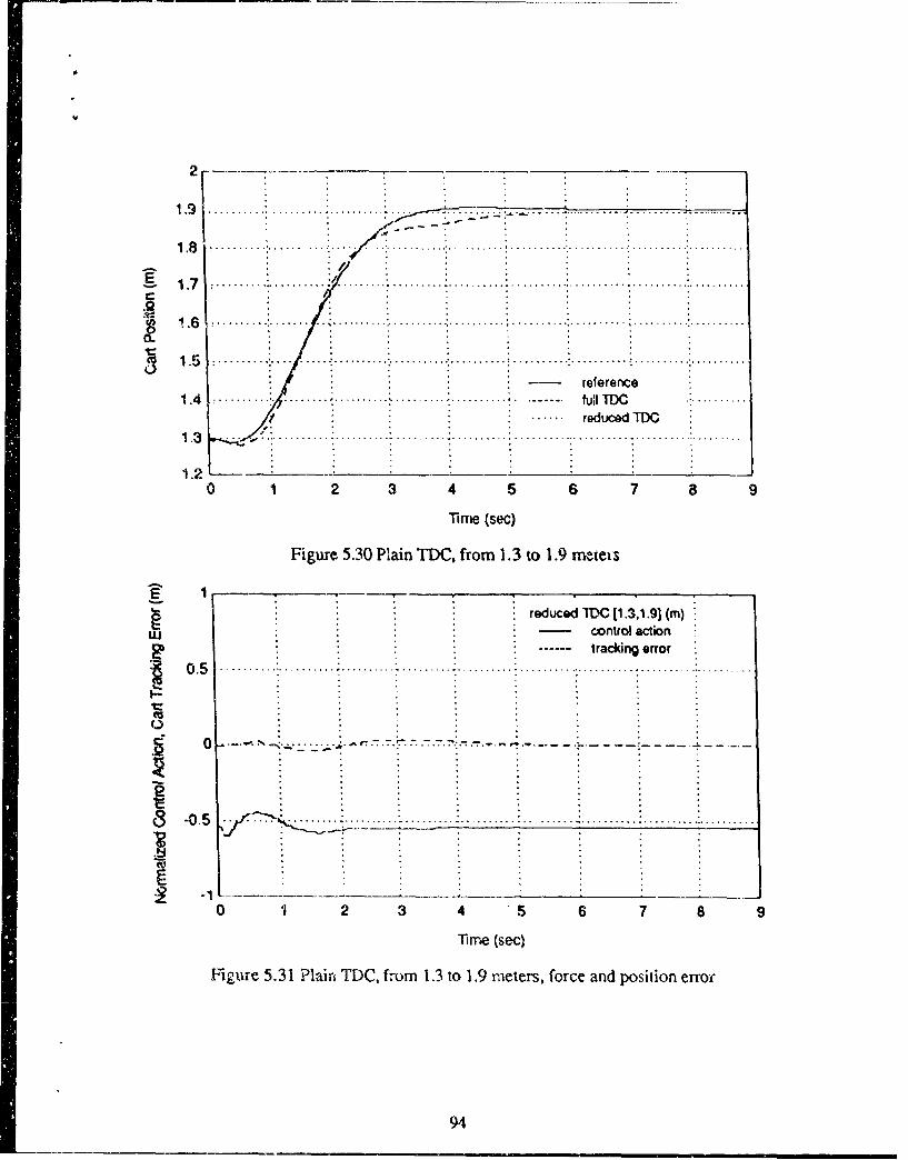
|2I.'

1 .7 .. . . . ... . . . .. . . . . . .. . . . .

1.5 . . - reference

1 .4 . . .. . . . . . - fu ll ... . .. . . . . ..... . . .

/ - reduced-C i1 . ... . . .:• - .. .. •..,.. .. .. i .. .. .. i ...... ... . . ..... . f l"T ,.!..........,] ,..'i + + + ............

1.2 _ - _:

0 1 2 3 4 5 6 7 8 9Time (sec)

Figure 5.30 Plain TDC, from 1.3 to 1.9 meters

E 1 - " . •--', •

reduced TDC 11.3,1.91 (m)control action

------. tracking error0 .5 ... .... .............. .......... ...... .. ....... .. ......

it

0

0 . .. ........ . . ... .. ..... .....................................

0 1 2 3 4 "5 6 7 8 9

Time (sec)

FHigure 5.31 Plain TDC, from 1.3 to 1.9 meters, force and position error

94

full TDC (1.3,1.91 (M)-control action

*~ 0.

- ... .. 0I. ........

0 1 2 3 4 5 6 7 8 9

"Time (sec)

Figure 5.32 Plain TDC, from 1.3 to 1.9 meters, force and position error

Sections 5.1 through 5.4 have explored several different approaches to combining

learned information with the adaptive controller. Using partial derivatives in the equation

seemed to be helpful, but only if the network was constrained to learn functions linear in x

and nonlinear in u. Using the reduced canonical fcorn had the advantage of allowing the

network to learn a function with one output instead of four. and worked well enough that

the partial derivatives were not needed. This system worked better for computation delays

and actuator dynamics, and worked equally well in the presence of noise. Overall, the full

hybrid u-;ing partial derivatives tended to be the most effective controller, especially when

the trajectory of the plant was largely in the region of greatest unmodeled dynamics.

95

It

5.7 COMPARISON OF CONNECTIONIST NETWORKS USED

5.7.1 Sigmoid

The network used in most of the above experiments was a Backpropagation, 2

hidden layer, sigmoid network. Each of the inputs and outputs of the network were scaled

before entering and after leaving it, so that each signal would vary over a range of unit

width, and the network would give equal preference to errors in each output. After trying

several different learning rates, it was found to learn best with a rate of 0.005. The

following graph shows the learning curve for the network while learning the function

P(x,u), where T was a nonlinear function of both x and u. The network output T is a

four element vector with one element for each of the four elements of state. The graph

shows the base 10 logarithm of the error in the network's output as a function of training

cycle.

96

Sernilog Plot of Error During Learning

*o- AI

ULo I O(x)

2.5%1

0 1 .34

Number of tralnlng examples (mlNions)Figure 5.32

Even though each point in the curve is the average error in the output over a period

of 400 training points, the curve still appears very noisy. This noise tends to cause the

network to forget what it has learned unless the learning rate is fairly low, and so this noise

is probably the reason that a learning rate of 0.005 was the largest learning rate that

converged to a local minimum. Higher learning rates changed the weights so much on

every step they changed enough to forget previously learned information. Lower learning

rates caused the network to learn even more slowly than in figure 5.32. The training period

shown in the figure took approximately 63 hours to run on a Macintosh IIfx. Figure 5.33

shows a 3 dimensional slice of the 6 dimensional surface learned. In the figure, the three

elements of state not shown are held at zero.

97

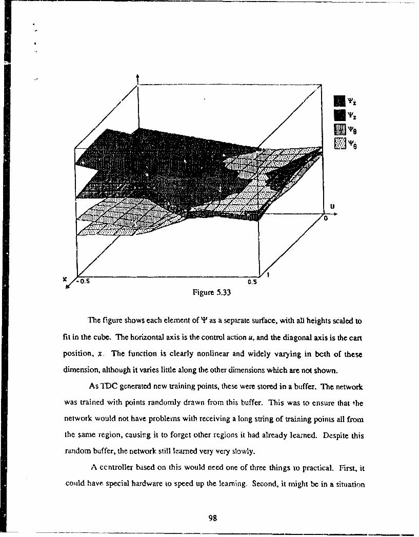
we

U;

Figure 5.33

The figure shows each element of TP as a separate surface, with all heights scaled to

fit in the cube. The horizontal axis is the control action u, and the diagonal axis is the cart

position, x The function is clearly nonlinear and widely varying in both of these

dimension, although it varies little along the other dimensions which are not shown.

As TDC generated new training points, these were stored in a buffer. The network

was trained with points randomly drawn from this buffer. This was to ensure that the

network would not have problems with receiving a long string of training points all from

the same region, causing it to forget other regions it had already learned. Despite this

random buffer, the network still learned very very slowly.

A ccntroller based on this would need one of three things to practical. First, it

could have s•ecial hardware to speed up the learning. Second, it might be in a situation

98

where long learning times are acceptable. Irfa factory rob 't can learn to adjust to normal

wear within a few days, then it should be able to learn the unmodeled dynamics fastc, than

it changes. Third, the algorithm ir'. the network might be modified to allow faster learning.

This third approach was taken here.

5.7.2 Sigrnoid with a Second Order method (Delta-Bar-Delta)

One attempt to speeding learning was to apply a pseudo-newton method to the

learning within the sigmoid network. Delta-Bar-Delta was -hosen because it requires very

little extra computation time, and it has con-pared favorably with a number of other

methods. Unfortunately, comparisons between methods for speeding !carning are often

done with benchmark problems that do not represent the problem here. People ofitn

compare learning speeds for learning an XOR function or a multiplexor function. These

can be difficult problems fer a network to learn, but the network has the advantage t'at the

set of training points is finite and small, so it is not unreasonable to change weights only

after each cycle irough Call the training data. Learning a function defined over a real vector

is more difficult, since there is an infinite set of training points. The function tended to ue

smooth and have few wrinkles, which meant that there was a large amount of redundancy

in the data which the learning algorithm shoulo be able to take advantage of. The fuiction

also contained discontinuities, however, (at the boundaries of the tilted track), so the

network nefeded to be able to handle that. All of these factors cornmined yielded a problem

which was slow for Backpropagation alone to learn, but should have been learnable

quickly by other learning methods.

When Delta Bar Delta was first applied, it immediately set all of the local learning

res to zero, causing the weights to freeze. T'his was because it worked by comparing the

current partial derivative of error with rsj,;ct to a given weight with au exponential average

of recent values of this de'vative. Since this was being done after every training point, it

saw the noise in the training data and interprcted that as rapidly changirng signs in• the error

99

derivatives. It responded to that by repeatedly decreasing all of the local learning rates.

This pioblem arose because Delta Bar Delta was not being used in an epoch training

mode as it had been designed for. The apparent solution was to calculate two exponentially

smoothed averages of the error partials. If these two averages had diffeicnt time constants,

then comparing them would be like comparing the current true derivative with slightly older

true derivatives.

The values for thesce time constants were chosen heuristically. Looking at the

learning curve for normal Backpropagation showed that the errors were noisy, but in a 500

training point period a "representative sample" of training points was probably being seen.

The short term average was therefore chosen so that 80% of the average was determined by

the last 500 training points. The long term average was then chosen to be 5 time.; slower,

basing 80% of its value on the last 2500 training points. In normal Delta Bar Delta, the

learning rate is increased by a constant every time the current derivative has the same sign

as the long term derivative average. Since this variation would update learning rates about

500 times more often, the rate of increase for learning rates was set 500 times smaller than

is suggested for normal Delta Bar Delta. Similarly, when learning rates are decreased, the

decrease is done exponentially by dividing by a constant each time. Since the modified

Delta Bar Delta would be expected to divide by this constant 500 times as often, the 500th

root of the sugge.sted constant was used.

There are two novel ways that Delta Bar Delta can fail. If local learning rates are

increased too often, then they get very large, and weights in the network can start to blow

up. On the other hand, if local learning rates are decreased too often, then they rapidly

approach zero, and the weights freeze. If the local learning rates stay in a reasonable range,

then Delta Bar Delta can succeed or fail in the same manner as Backpropagation, although

hopefully it reaches the final state faster.

In experimenting with Delta Bar Delta, every run either had exploding weights or

vanishing learning rates. Given the very noisy training data that the network was exposed

100

to, I was unable to find a useful set of parameters for Delta Bar Delta. It is, of course,

pcssible that such a set of parameters exists, but after repeated tries " could not find them.

Perhaps Delta Bar Delta would work better if all the local learning rates were normalized on

each time step to keep a constant average value. Perhaps some other heuristic might be

applied. It is not immediately clear what would be the best way to deal with this problem.

101

6 CONCLUSIONS AND RECOMMENDATIONS

6.1 SUMMARY AND CONCLUSIONS

This thesis has described a new method for integrating an indirect adaptive

controller with a learning system to form a hybrid controller, combining the advantages of

each system. When a learning system is trained with the estimates found by the adaptive

conttroller, the hybrid system reacts more quickly to unmodeled spatial nonlinearities in the

plant. This system follows a reference trajectory better than the adaptive controller alone,

but it can still be improved upon. By using a connectionist system to learn the function, it

is easy to calculate the partial derivatives of that function, which in turn allows better

estimates of unmodeled dynamics, and better estimates of the effect of control action on

state. This modified controller performed better than either the adaptive controller alone or

the original hybrid system.

The feedforward, sigmoid learning system was able to leant the required functions

accurately, but he the learning tended to be slow. The problem of slow convergence is

widely recognized and is dealt with by methods such as Delta-Bar-Delta, which speed

learning a great deal in published experiments. Unfortunately, those problems used for the

comparisons usually involve small sets of training examples. The learning problem which

arose in this thesis theoretically required an infinite training set. In practice, Delta-Bar-

Delta was found to be very sensitive to the choice of parameters. Even modifying Delta-

Bar-Delta to use two traces instead of one did not solve this problem, and it actually

introtduced another parameter which had to be chosen. Therefore methods for speeding

convergence on small test problems do not appear to scale as well as commonly thought.

102

6.2 RECOMMENDATIONS FOR FUTURE WORK

The desired refere'nce trajectory used in these experiments was chosen manually to

give fairly fast response while still being achievable with the 10 Newton force constraint on

the controller. It would be de&,rable to to automate the choicr' of reference, and this may be

possible. The reference trajectory could start off as a poc .. ontroller which is achievable

witt;out using much force. It could then be slowly improved automatically until the

actuators saturate, thus finding the best reference which can be matched by this hybrid

controller architecture. The reference could even be a function of state, stored in a separate

connectionist network.

The learning systems used here learned very good approximations, but the learning

tended to be slow. The Delta-Bar-Delta algorithm improves the rate of convergence for

small sets of training points, but was not effective for learning as part of a hybrid control

system, even after being modified. It tended to be too sensitive to the choice of parameter.

Learning based on following the first derivative should be faster if accurate measurements

of the seconds derivative can be found, so a system such as Delta-Bar-Delta should be

useful if it can automate the choice of parameters, perhaps based on an estimate of how'

accurate its second derivative citimates are. Further research should focus on this problem,

perhaps by measuring the standard deviation of the individual measurements to form an

estimate of the accuracy of their average.

103

BIBLIOGRAPHY

[Ast83] Astr~m, K., "Theory and Application of Adaptive Control - A Survey,"Automatica, Vol. 19, No. 5, 1983.

[BB90] Baird, L. and W. Baker, "A Connectionist Learning System for NonlinearControl," Proceedings, AIAA Conference on Guidance, Navigation, andControl, Portland, OR, August, 1990.

[BF90 Baker, W. and J. Farrell, "Connectionist Learning Systems for Control,"Proceedings, SPIE OE/Boston '90, (invitcd paper), November, 1990.

[Bar89] Barto, A., "Connectionist Learning for Control: An Overview," COINSTechnical Report 89-89, Department of Computer and Infonration Science,University of Massachusetts, Amherst, September, 1989.

[BS90] Barto, A., and S. Singh, "Reinforcement Learning and DynamicProgramming," Proceedings of the Sixth Yale Workshop on Adaptive andLearning Systems, New Haven, CN, At,iqst. 1990.

[BSA'3] Barto, A., R. Sutton, and C. Anderson, "Neuronlike Adaptive Elements ThatCan Solve Difficult Learning Control Problems," IEEE Transactions onSystems, Man, and Cybernetics, vol. SMC-13, No. 5, September/October1983.

[BSW891 Barto, A., R. Suttcv, and C. Watkins, "Learning arcd "equential DecisionMaking," COINS 1echnical Report 89-95, Department of Computer andInformation Science, Univers'ty of Massachusetts, Amherst, Septemtrnr, 19R.

[D'A88] D'Azzo, J., Linear Control System Analysis & Design: Conventional andModern, McGraw-Hill, New-York, 1988.

[FGG90] Farrell, J., Goldenthal, W., and K. Govindarajan, "Connectionist LarniirgControl Systems: Submarine Heading Control," Proceedings, 29th IEEEConference on Decision and Control, December, 1990.

[Fu86] Fu, K., "Learning Control Systems - Review and Outlook," IEEE Transactionson Pattern Analysis and Machine Intelligence, vol. PAMI-8, No. 3, May, 1986.

[GF90] Goldenthal, W. and J. Farrell, "Application of Neural Networks to AutomaticControl," Proceedings, AIAA Conference on Guidance, Navigation, andControl, August, 1990.

[HW891 Hornik, K., and M. White, "Multilayer Feedforward Networks are UniversalApproximators," Neural Networks, Vol. 2, 1989.

[Jac9l] Jacobs, R., "Increased Rates of Convergence Through Learning Rate

Adaptation," Neural Networks, 1,2, p. 295-301, 1991.

[Jam9OI Jamiesori, J., "A Neurocornputer Based on Model Feedback and the Adaptiveileuiistic Critic," Proceedings of the International Joint Conference on NeuralNetworks, 1990,,

[.Jor881 Jordan, M., "Supervised Learning and Systems with Excess Degrees ofFreedom," Technical Report COINS TR 88-27, Massachusetts Institute ofTechnology, 1988.

[Klo88] Klopf, H., "A Neuronal Model of Classical Conditioning," Psychobiology,vol. 16 (2), 85-125, 1988.

[LeC87] LeCun, "Modeles Connexionnistes le l'Apprentissage," Ph.D Thesis,Universite Pierre et Marie Curie, Paris, 1987.

[MC68] Michie, D., and R. Chambers, "Boxes: an Experiment in Adaptive Control,"Machine Intelligence, vol. 2, E. Dale and D. Michie, Eds., Edinburgh,Scottland: Oliver and Boyd Ltd., 1968.

[Mi19 11 Millington, P., "Associative Reinforcement Learning for Optimv~d Control,"Master's Thesis, Massachusetts Institue of Technology, 1991.

[M.P691 Minsky, L. and S. Papert, Percepirons, MIT Press, Cambridge, MA, 1969.

11NW89] Nguyen, D., and B. Widrow, "The Truc-k Backer-Upper An Example of Self-Learning in Neural Networks," Proceedings of the International JointConference on Neural Networks, 1989.

[Pa1831 Palm, W., M'odeling,. Analysi~s, and Control of Dynamic Systems, Jfohn Wiley& Sons, Newv York, 1983.

[Par821 Parker, D., 'Learning Logic," Invention Report, S81-64, File 1, Office ofTechnology Liscensirig, Stanford University, 1982.

[Ros62J Rosenblatt, F., Principles of Neurodynamics, Spartan Books, Washington,1962.

[RZ.86] Rumnelbart, D. and D. Zipser, "Feature Discovery by Competitive Learning,"Par~allel Distributed Processing: Explorations in the Microstructure ofCognition, vol. 1, Rumelhart, D., and J. McClelland, ed., MIT Press,Carbnbdge, MA, 1986.

[RI-1W86] Rumnelhart, D., 0. Hinton, and R. Williams, "L~earning Internal Representationby Error Propagation," Parallel Distribwled Processing: Explorations in theMicrostructure of Cognition, vol. 1, Rumelhart, D., and J. McClelland, ed.,MIT Pres, Cambridge, MA, 1986.

[Sain67] Samuel, A., "Some Studies in Machine Learning Using the Game of Clieckers11 - Recent Progress," IBM Journal of Research nod Development, 11,601-617,1967.

[Sarn591 Samuel, A., "Some Studies in Machine Learning Using the Game ofCheckers," IBM Journal of Research and Developm-ent, 3, 2 10-229, 1959,

reprinted in Computers and Thought, A. Feigenbaum and J Feldman,ed.,McGraw-Hill, New York, 1959.

[Sim87] Simpson, P., '"A Survey of Artificial Neural Systems"," Technical Dcx:ument1106, Naval Ocean Systems Center, San Diego, CA, 1987.

[Sut90] Sutton, R., "Artificial Intelligence by Approxima~ing DynamicProgrammning," Proceedings of the Sixth Yale Workshop on Adaptive andLearning Systems, New Haven, CN, August, 1990.

[Sut88] Sutton, R., "Learning to Predict by the Methods of Temporal Differences,"Machine Learning, KlNwIr Academic Publishers, Boston, MA, vol. 3: 9-44,1988.

[Wat89] Watkins, C., "Learning trom Delayed Rewards," Ph.D, thesis, CambridgeUniversity, Cambridge, England, 1989.

[Wer89] Werbos, P., "Backpropagation and Neurocontrol: A Preview and Prospectus,"Proceedings of the International Joint Conference on Neural Networks,Washington, D.C., pp. 209-216, vol. 1, 1989.

[Wer74] Werbos, P., Beyond Regression: New Tools for Prediction an'rd Analysis in :heBehavioral Sciences, PhD Dissertation, Harvard University, 1974.

[Wid89] Widrow, B., "'ADALINE and MADALINE," Proceedings of the InternationalJoint Conference on Neural Networks. 1989.

[WZ89] Williams, J. and D. Zipser, "A Learning Algorithm for Continually RunningFully Recurrent Neural Networks," Neural Computation, 1, 270-280, 1989.

[WB90] Williams, R. and L. Baird, "A Mathematical Analysis of Actor-CriticArchitectures for Learning Optimal Controls Through Incremental DynamicProgramming," Proceedings .'9f the Sixth Yale Workshop on Adaptive andLearning Systems, New Haven, CN, August, 19.9.

[Wil88] Wiliarns, R., "Towards a Theory of Reinforcement Learning ConnectionistSystems," Technical Report NU-CCS-88-3, College of Computer Science,Northeastern University, July, 1988.

[YI90] Youcef-Toumi, K. and 0. Ito, "A Time Delay Controller for Systems withUnknown Dynamics," ASME Journal of Dynamic Systems, Measurement, andConti!l, Vol. 112, March, 1990.