
Drug Innovations and Welfare Measures Computed from …
33
Drug Innovations and Welfare Measures Computed from Market Demand: The Case of Anti-Cholesterol Drugs Abe Dunn December 13, 2011 Abstract The pharmaceutical industry is characterized as having substantial investment in R&D and a large number of new product introductions, which poses special problems for price measurement caused by the quality of drug products changing over time. This paper applies recent demand estimation techniques to individual level data to construct a constant-quality price index for anti-cholesterol drugs. Although the average price for anti-cholesterol drugs does not change over the sample period, I nd that the constant-quality price index drops by 27 percent, a pace more in line with our expectations in such a dynamic segment of the industry. 1 Introduction The growth in medical technology is a driving force behind the rising costs of medical care, ac- counting for as much as 50 percent of cost growth in recent decades. 1 Although new technologies I would like to thank Ana Aizcorbe, Ralph Bradley, Gautum Gowrisankaran, John Greenlees, Chuck Romeo, Adam Shapiro, Brett Wendling and seminar participants at the Bureau of Labor Statistics for comments. I would also like to thank Karen Rasmussen M.D. for sharing her knowledge about cholesterol treatment. This paper also beneted from comments by Randal Watson, Stephen Donald, and Ken Hendricks on an earlier version of this paper. Sarah Pack provided research assistance. The views expressed in this paper are solely those of the authors and do not necessarily reect the views of the Bureau of Economic Analysis. 1 Based on studies by Newhouse (1992), Cutler (1995), and Smith et al. (2000), the Congressional Budget O¢ ce (2008) estimates that new technologies account for approximately 50 percent of cost growth in medical care in recent 1
Transcript of Drug Innovations and Welfare Measures Computed from …

Drug Innovations and Welfare Measures Computed from
Market Demand: The Case of Anti-Cholesterol Drugs�
Abe Dunn
December 13, 2011
Abstract
The pharmaceutical industry is characterized as having substantial investment in R&D
and a large number of new product introductions, which poses special problems for price
measurement caused by the quality of drug products changing over time. This paper applies
recent demand estimation techniques to individual level data to construct a constant-quality
price index for anti-cholesterol drugs. Although the average price for anti-cholesterol drugs
does not change over the sample period, I �nd that the constant-quality price index drops
by 27 percent, a pace more in line with our expectations in such a dynamic segment of the
industry.
1 Introduction
The growth in medical technology is a driving force behind the rising costs of medical care, ac-
counting for as much as 50 percent of cost growth in recent decades.1 Although new technologies
�I would like to thank Ana Aizcorbe, Ralph Bradley, Gautum Gowrisankaran, John Greenlees, Chuck Romeo,
Adam Shapiro, Brett Wendling and seminar participants at the Bureau of Labor Statistics for comments. I would
also like to thank Karen Rasmussen M.D. for sharing her knowledge about cholesterol treatment. This paper also
bene�ted from comments by Randal Watson, Stephen Donald, and Ken Hendricks on an earlier version of this paper.
Sarah Pack provided research assistance. The views expressed in this paper are solely those of the authors and do
not necessarily re�ect the views of the Bureau of Economic Analysis.1Based on studies by Newhouse (1992), Cutler (1995), and Smith et al. (2000), the Congressional Budget O¢ ce
(2008) estimates that new technologies account for approximately 50 percent of cost growth in medical care in recent
1

may lead to higher expenditures on medical care, they also a¤ect the quality of treatment, typically
improving patient welfare and lowering the quality-adjusted cost of treatment.2 The rapid shift
in product quality over time poses special challenges for price measurement. In the medical care
sector, price index estimates that hold quality �xed are critical for measuring real output and may
also inform public policies related to innovation.3
This paper focuses on the measurement of prices for anti-cholesterol drug treatments, which is
one of the more important areas of innovation in the pharmaceutical sector over the past three
decades. Extensive medical evidence has shown that high cholesterol is a contributing factor in 56
percent of the cases of clinical heart disease, which is the leading cause of death in the United States.
The introduction of the statin class of cholesterol-lowering drugs starting in 1987 has proven to be
a key development for preventing heart disease.4 Innovations in this area have led to rapid growth
in this market, with the use of anti-cholesterol medications increasing more than 400 percent over
the period of study from 1996 to 2007.
This paper uses a demand model for anti-cholesterol drugs to construct a price index that
accounts for quality changes resulting from new product introductions. The approach applied in
this paper has been used to assess the value of new goods in a variety of industries.5 However,
relatively few papers have applied these techniques to examine the impact of innovations in the
medical care sector. One of the seminal papers examining innovation in the medical care industry
is Trajtenberg (1989) that looks at the CT scanner market. More recent work has focused on the
pharmaceutical industry with Cleanthous (2004) studying innovations in the market for depression
drugs and Lucarelli and Nicholson (2009) looking at new colorectal cancer drugs.
decades. A more recent study by Smith et al. (2009) estimates that medical technology explains 27-48 percent of
health spending growth since 1960.2For example, see Cutler et al. (1998), Cutler and McClellan (2001), and Berndt et al. (2002).3If the price index falls as innovative products enter the market, then this would suggest that innovations have led
to improved treatments, relative to the cost, and we should continue supporting policies that promote innovation.
Conversely, if the price index increases when new products enter the market, then one might conclude that innovations,
in some sense, were not worth the cost.4Many individuals with high cholesterol can expect to gain many months or years of additional life by using statin
treatments. The U.K. study by Ward et al. (2007) and the Heart Protection Study Collaboration Group (2010)
provide nice reviews of the literature looking at statin drug e¤ectiveness.5The areas of study include automobiles (Berry, Levinsohn, and Pakes (1993) and Petrin (2002)), computers
(Greenstein (1996)), and breakfast cereals (Nevo (2003)). For a more complete review of the literature see Bresnahan
and Gordon (1997).
2
In this paper, the demand for anti-cholesterol drugs is modeled using a discrete-choice framework
similar to Berry (1994) and Berry, Levinsohn, and Pakes (1995; henceforth BLP). In contrast to
the previous work that uses aggregate data to examine innovations in the medical care sector, the
model presented here uses detailed, nationally representative individual-level data that includes
information on health conditions, demographics, health insurance, drug insurance, and individual-
speci�c drug choices. The model permits �exible substitution patterns that are a¤ected by the
observed health conditions and demographics of individuals in the market. This model is particularly
well-suited for estimating the welfare from new medications since the e¤ectiveness of drugs and their
side e¤ects may vary depending on the severity of the condition, the speci�cs of the disease, and
other demographic factors. If individual health conditions are not observed it may be di¢ cult to
separately identify a demand increase resulting from an improvement in the quality of a drug from
one caused by the growing prevalence or awareness of a condition. Using individual level information
on drug insurance coverage I am also able to control for potential moral hazard e¤ects that may
distort the market valuation of anti-cholesterol drugs. Many papers, including Gaynor and Vogt
(2003), Petrin (2002), and Goolsbee and Petrin (2004), have found the use of consumer level data
to vastly improve di¤erentiated product demand estimates.
The results indicate that the quality-adjusted price of anti-cholesterol drugs has fallen consid-
erably since 1996, re�ecting the importance of innovation in this market. Relative to the CPI,
the quality-adjusted price fell by 9 percent from 1996 to 2005, while the average price grew by 37
percent and a Laspeyres index (similar to that used by the Bureau of Labor Statistics (BLS)) grew
by 9 percent. Both the average price and the quality-adjusted price fell sharply after 2005 following
the entry of generics. The decline in quality-adjusted price observed over the study period is large,
but likely understates the decline that has occurred over a longer horizon. In fact, much of the
innovation in the market may be attributable to the introduction of statin drugs that were available
prior to the study period, which accounted for 72 percent of consumer welfare in the initial year of
this study.
The next section describes the market for anti-cholesterol drugs. Section 3 presents the model.
Section 4 describes the data, followed by a discussion of the results in section 5. Section 6 concludes.
3
2 The Market for Anti-Cholesterol Drugs in the United
States
The World Health Organization (2002) reports that high cholesterol causes 4.4 million deaths in
the world each year. High cholesterol continues to be a prevalent and serious health condition, but
signi�cant improvements have been made in the treatment of high cholesterol over the last forty
years. According to estimates from the Centers for Disease Control and Prevention, 28 percent of
individuals over 20 had high cholesterol in the late 1970s. That �gure is around 16.3 percent today
and much of the decline is likely attributable to the introduction of new cholesterol-lowering drugs
and an increase in the number of individuals being treated.6 There is particularly rapid growth
in both the awareness of high cholesterol and the use of anti-cholesterol medication from 1996 to
2007. The percentage of people 20 or older that report having high cholesterol has increased from
3.5 percent in 1996 to 17.2 percent in 2007.7 In addition to a growth in the number of individuals
reporting high cholesterol, there has also been a substantial increase in the fraction of individuals
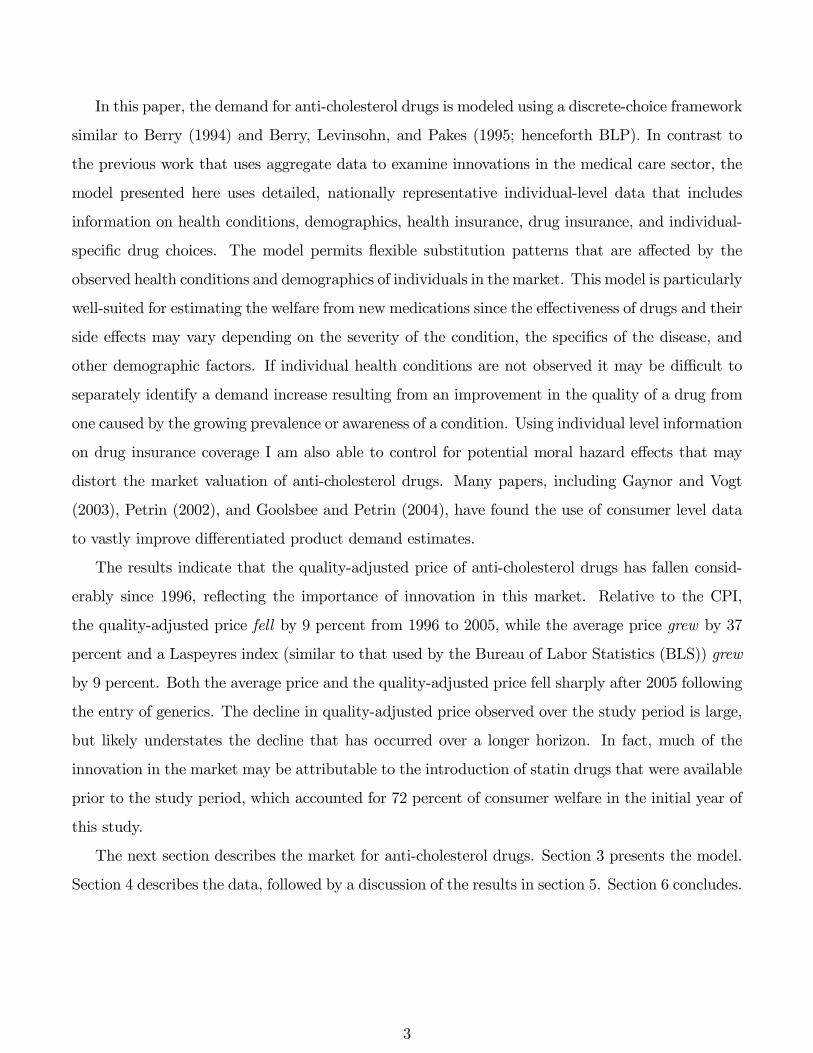
with high cholesterol using anti-cholesterol medication, as shown in Figure 1.
[Figure 1. The Fraction of Individuals with High Cholesterol Over 20 that Use an Anti-
Cholesterol Drug ]
Several factors have contributed to the growing use of anti-cholesterol medications. First, mount-
ing clinical evidence strongly links high cholesterol and heart disease, and veri�es the e¤ectiveness
of cholesterol-lowering treatments to reduce heart disease. The development of more e¤ective drugs
and the introduction of several low-priced generics may have also increased patient usage of anti-
cholesterol drugs. Increases in the level of advertising for these drugs, and the consequent increase
in public awareness of high cholesterol as a serious health condition, may also be a factor.
This study looks at the full spectrum of anti-cholesterol drug treatments, including some that
have been around for more than four decades. There are �ve classes of drugs used to treat high
cholesterol including: nictonic acid derivatives, �bric acid derivatives, bile acid sequestrants, ez-
itimbe, and statins. While medications in each of these drug classes can lower cholesterol, the
6These statistics are reported in Health United States (2009). High cholesterol is de�ned as serum cholesterol
levels of 240 or higher. The estimates are based on actual cholesterol readings, which include the e¤ects of medication
on cholesterol levels.7These �gures are from the MEPS data, discussed in greater detail in the data section. These estimates include
individuals that would have high cholesterol if they were not taking cholesterol lowering treatment.
4
introduction of the statin class of anti-cholesterol drugs in the 1980s has been revolutionary for the
treatment of high cholesterol. Statin drugs have several advantages: they are easy to administer,
have few side e¤ects, and are the most e¤ective at lowering LDL or �bad�cholesterol, the primary
target of drug therapy according to the National Cholesterol Education Program (2001). These
factors led statins to become the top selling class of drugs in the U.S. during the period between
1999 to 2008.8 Compared to other cholesterol treatments, statin drugs are relatively new; the �rst
drug in this class, Mevacor, was introduced in 1987. Several drugs have entered the statin class since
then, including Pravachol, Zocor, Lescol, Baycol, Advicor, Vytorin, Lipitor, and Crestor. Table 1
below shows market shares of the various statin drugs from 1996 to 2007, along with the market
share of non-statin medications. A key event during the period of study was the entry of Lipitor
in 1997, which became the top selling drug in the U.S. by 1999 and remained the top selling drug
over the next decade.9 At the time of Lipitor�s entry into the market it was the most e¤ective drug
for lowering LDL cholesterol. Another important shift in cholesterol treatments has been the intro-
duction of generic statins, including the generic version of Mevacor, which lost patent protection in
2002, and the generic versions of Pravachol and Zocor, which lost patent protection in 2006.10
[Table 1. Market Shares of Users of Cholesterol Drugs - MEPS Data]
In general, the non-statin medications are less e¤ective at reducing LDL cholesterol and have
more severe side e¤ects than the drugs in the statin class; consequently the market share of these
other drugs has declined from its 21 percent high in 1996 and has not exceeded 11 percent since 1998.
Table A1 in the appendix displays attributes of anti-cholesterol drugs related to the e¤ectiveness
of each drug at lowering cholesterol. For example, it shows that Lipitor and Crestor are the most
e¤ective at lowering LDL cholesterol.11 Table A1 also shows that higher doses of the drugs tend to
be more e¤ective, but higher doses also tend to come with more severe side e¤ects. There are many
di¤erences among anti-cholesterol drug treatments, but there is also an idiosyncratic component to
the quality of these drugs, so that some individuals may respond better to certain drug treatments
8Matthew Herper, �Statins Dethroned,�Forbes, March 30, 2009.9From IMS Health pharmaceutical sales estimates.10Generic manufacturers can legally o¤er new products in a market using the active molecule of a drug when its
patent expires.11There are many attributes not shown in Table A1. Drugs may also di¤er in their side e¤ects (e.g. muscle pain
or liver damage) and proven e¤ectiveness based on clinical outcomes. For instance, Zocor was one of the �rst drugs
shown to be e¤ective in clinical trials at reducing cardiovascular deaths. See the Scandinavian Simvastatin Survival
Study (1994).
5
relative to others taking the same medication.
Another important feature of anti-cholesterol drugs is their pricing. Figure 2 demonstrates
di¤erences in pricing across medications and over time. The bold line in Figure 2 shows the overall
average price of a daily dose of treatment, where a daily dose is a single pill. Figure 2 also shows
pricing trends for speci�c daily dose treatments, such as the 10 mg dose of Lipitor and the 10
mg dose of Zocor.12 The overall average price from 1996 to 2005 grew substantially because of a
growing demand for newly introduced drugs that tend to be more expensive. In addition, prices
have trended upward on many of the more popular drugs (i.e. Lipitor, Zocor, and Pravachol). For
much of the sample period, the most popular branded drugs had an unexpired product patent and
did not face generic competition. As a result, generic �rms could not enter the market, and average
prices remained relatively high at around $2 to $3 per pill for most statins. The introduction
of generic versions of Zocor and Pravachol in 2006, with prices 75 percent less than the branded
versions, led to a dramatic decline in the average price in 2006 and 2007.
[Figure 2. Drug Prices For Selected Cholesterol Drugs and Market Average Price]
Figure 1 and Figure 2 present con�icting descriptive evidence regarding welfare changes. If
Figure 1 is viewed as a quantity index then one might infer, through revealed preference, that
individuals are better o¤ in 2005 than in 1996 because more individuals with high cholesterol are
taking anti-cholesterol medications. On the other hand, looking at the increase in average price in
Figure 2, one might conclude that welfare has declined. The quality-adjusted price index derived
from market demand, constructed in this paper, may be viewed as an approach for weighing the
relative importance of price and quality changes.
3 Econometric Model of Demand
In contrast to most purchasing decisions, in prescription drug markets individuals rely on their
doctors to tell them which drug, if any, is best suited to treat their condition. At the same time,
the insurer induces price sensitivity through the structure of the insurance plan, which is important
since the full price of the selected drug ultimately has an e¤ect on premiums. For these reasons, one
might view the choice of the prescription drug as a joint decision of the individual, the insurer, and
12The overall average price is greater than those for the selected drugs because many of the more expensive higher
dose treatments are not shown in Figure 2.
6

the physician. In the case where the doctor and insurer act in the best interest of the individual, the
individual is able to optimally choose a medication. This is the maintained assumption throughout
the presentation of the model. However, to the extent that market distortions are present, then the
model below will only be an approximation to individual utility, and may be more appropriately
viewed as a market demand function.
In every period each individual chooses a product that maximizes her utility. The set of options
is f0; :::; Jtg where Jt is the number of products available in period t. Here the option 0 is the choice
not to take a drug. Individual i chooses option j 2 f0; :::; Jtg in period t if uijt > uikt 8k 6= j, and
each individual only chooses one option. I assume that individual i�s indirect utility for product j
where, j 6= 0; at time t is given by uijt = �itpjt+�itxjt+ �jt+ �ijt where pjt is the price of drug j in
period t, xjt is the vector of characteristics of drug j in period t, �jt is the value of the unobserved
(by the econometrician) product characteristic, and �ijt is the idiosyncratic component of individual
i�s indirect utility for drug j. The indirect utility of the outside good is normalized to be zero.
The response of individual i to the price and product characteristics consists of a component that
is common to all individuals and a component that depends upon her observed characteristics, zit,
so that �it = �0 + �1zit and �it = �0 + �1zit. For example, the health conditions of the patient
enter the model through zit. Thus, the indirect utility of each product may be decomposed into a
mean component, �jt = �0pjt + �0xjt + �jt, that is common to all individuals in the sample, and a
component that is individual speci�c, �1zitpjt + �1zitxjt + �ijt.
Estimating Equations: To estimate the above model using micro-level data, I follow the approach
outlined in Berry, Levinsohn, and Pakes (2004). The estimation procedure has two stages. In the
�rst-stage, the mean component of utility is estimated along with the individual speci�c parameters.
For this �rst-stage, I assume that �ijt takes on an extreme value distribution, so the probability of
choosing option j takes the logit form:
Probit(jjz; x; �; �; �) =exp(�jt + �1zitpjt + �1zitxjt)
�Jtk=0exp(�kt + �1zitpkt + �1zitxkt): (1)
Equation (1) is estimated by maximum likelihood, which identi�es the �1 and �1 vectors of para-
meters along with mean utility, �jt.13 The mean utility is then used as a dependent variable in the
second-stage estimation, where mean utility is regressed on price and drug characteristics:
13Note that when one has individual level data, then �jt may be estimated directly using maximum likelihood, so
it is not necessary to solve for �jt as is typical when only aggregate level data is available.
7

�jt = �0pjt + �0xjt + �jt: (2)
When estimating the second-stage, the issue of price endogeneity is addressed using both drug-
strength �xed e¤ects and instrumental variables.14
Instruments: It is often challenging to �nd valid instruments that a¤ect a �rm�s pricing strategy,
but are uncorrelated with unobserved product characteristic, �jt. Common instruments are factors
that a¤ect marginal cost, but the marginal cost of production is typically low for pharmaceuticals
and is likely to have a limited impact on price setting strategies. For this reason, an alternative
instrumental variable (IV) strategy is applied that exploits the detailed micro-level data and the
�rst-stage demand estimates.
The instruments are constructed using the �rst-stage logit estimates to predict market demand,
but with drug prices and the unobserved product characteristic set to zero (i.e. the potentially
endogenous terms are removed). The instruments formed from the �rst-stage demand estimates
include linear predictions of demand, but also nonlinear functions of demand that may capture
di¤erent aspects of the potential pricing strategies of �rms. For instance, price may be chosen
based on a markup term that depends on both the demand for the product and the derivative of
demand with respect to price, markup = pjt � mcjt =Djt@D
jt@pjt
. Both the demand function and the
derivative may be calculated by summing individual demand predictions and individual responses
to price. Speci�cally, the market demand for product j at time t is calculated as:
Djt =IXi=1
Probit(jjz; x; �; �; �) =IXi=1
exp(�jt + �1zitpjt + �1zitxjt)
�Jtk=0exp(�kt + �1zitpkt + �1zitxkt); (3)
and the responsiveness to price is measured as:
@Djt
@pjt=
IXi=1
@Probit(jjz; x; �; �; �)@pjt
: (4)
Instruments are constructed by using equations (3) and (4) to calculate predicted demand and the
predicted markup where �it = 0 and �jt = 0:
14Although it appears that the model could potentially be estimated using a simple conditional logit model, it is
likely that the price variable will be endogenous. In fact, several studies have found evidence of price endogeneity,
despite using micro level data, including Villas-Boas and Winer (1999), Gaynor and Vogt (2003), Goolsbee and Petrin
(2004), and Chintagunta et al. (2005).
8
DIjt(jjz; x; � = 0; � = 0; �); (5)
DIjt(jjz; x; � = 0; � = 0; �)
@DIjt(jjz;x;�=0;�=0;�)
@pjt
: (6)
Since generics often compete with other generics and may also have costs that are di¤erent from
the branded �rm�s, a second set of instruments is constructed by interacting a generic dummy with
the two instruments, genericjt � DIjt and genericjt �
DIjt
@DIjt
@pjt
. One might expect the branded products
with greater predicted demand to have higher prices; while generic products with greater predicted
demand may have more entry and lower prices.15
The basic idea behind this IV strategy is that an individual�s choice is a¤ected by her speci�c
demographic characteristics when selecting a product, as re�ected in the �rst-stage choice model.
However, individual information is conditioned out of the model in the �rst-stage, so it should not
enter the mean unobserved component of demand, �jt. Therefore, individual demographics will not
be correlated with mean unobserved demand; but the aggregate preferences of individuals in the
market should be correlated with the price because pro�t maximizing �rms will consider the overall
market demand (including population characteristics) when setting price.
A similar set of instruments was applied by Gaynor and Vogt (2003).16 This approach is also
related to the common strategy of using product characteristics to instrument for price as in BLP
(1995) because they both depend on consumer preferences and are impacted by the consumer�s
value of the product attributes. Rather than using product characteristics to predict price, this
15While the above strategy is the approach used in the main estimates of the paper, the appendix of the paper
shows that the estimates are robust to the chosen instrumenting strategy. This includes estimates that exclude the
markup terms from the set of instrumental variables and another robustness check that is not based on �rst-stage
demand estimates. One reason for checking alternative instrumenting strategies is that one may be concerned with
using �rst-stage demand estimates if manufacturers are able to price discriminate based on population demographics.
This type of price discrimination could potentially violate the assumption that the instruments are uncorrelated with
�jt.
One complication with constructing the estimate for@DI
jt
@pjtis that it depends on �, which is not observed. To
address this problem I estimate an alternative demand model where I use DIjt and D
Ijt � genericjt to instrument for
price. I then use the estimate of � from this IV regression to obtain an estimate of@DI
jt
@pjt.
16Another example is Romeo (2010) that uses consumer demographics as instruments in a discrete-choice model
with random coe¢ cients using aggregate data.
9

approach uses the predicted consumer preferences for the di¤erent drug treatments.
3.1 Quality-Adjusted Price Measures
The quality-adjusted price index in this paper is based on the changes in the compensating variation
derived from the estimated demand model. The compensating variation provides a measure of how
much income would need to change across the two periods to leave individuals indi¤erent between
the old choice set and the new choice set. Given the logit functional form, the compensating
variation from period t� 1 to period t for individual i is calculated as �Wit =E(uit)�E(uit�1)
�it, where
E(uit) is the unconditional indirect utility and �it is the marginal utility of income. The value of
the unconditional indirect utility is computed by integrating over the extreme value distribution.
Using the derivation of McFadden (1981), the unconditional compensating variation is calculated
as:
�Wit =
ln(JtXj=0
exp(�itpjt + �itxjt + �jt))� ln(Jt�1Xj=0
exp(�itpjt�1 + �itxjt�1 + �jt�1))
�it: (7)
As described in greater detail by Trajtenberg (1990), the compensating variation can be con-
verted into a price index by solving for the factor by which all prices are multiplied in period t in
order to get the same welfare e¤ect as �Wit for each individual. More precisely, given the change
in welfare, �Wit, from (7), the change in the quality-adjusted price is calculated by solving for 'it
such that:
�Wit =
ln(JtXj=0
exp(�itpjt � (1 + 'it) + �itxjt + �jt))� ln(JtXj=0
exp(�itpjt + �itxjt + �jt))
�it:
If welfare increases across the two periods, then 'it will be a negative value; and if welfare decreases
across the two periods, then 'it will be a positive value. The index will be speci�c to each individual
in the data and depend on her observed characteristics.17 To solve for the value of 'it an iterative
17The price index used here depends on the current period prices and product characteristics, which produces more
conservative estimates that tend to understate the reductions in quality-adjusted price from innovation, relative to
an alternative measure that uses the base period prices and product characteristics. Theoretically, using the base
10

search procedure is applied for each individual. An aggregate price index is constructed by averaging
over individual price changes.18
Work by Nevo (2003) suggests that researchers should exercise caution when using market
demand to construct quality-adjusted prices. He shows that the demand for breakfast cereals may
be impacted by whether unobserved demand, �jt, and trend variables are treated as changes in the
�taste�for a product or changes in actual product attributes. In particular, one might be concerned
that there is simply a growing trend in the treatment of high cholesterol that represents a growing
�taste�for anti-cholesterol medications, although the products (and studies on the e¤ectiveness of
the products) have not changed. If changes in the trend or �jt represent changes in the �taste�
of the product, then they should not be allowed to vary when conducting welfare analysis. On
the other hand, if these values capture unobserved quality changes, then they should be allowed
to vary. Although it is practically impossible to determine the correct assumption, I attempt to
address the importance of this issue by examining alternative estimates, including estimates that
allow the trend variable and the mean unobserved utility to vary and other estimates that hold
these values �xed over time.
The presence of drug insurance creates another concern. Drug insurance may cause a divergence
between the private value of a product and its social value because of a moral hazard e¤ect. To
explore the impact of drug insurance on quality-adjusted prices, I remove the e¤ects of drug insur-
ance from individual demand. I will explore how alternative assumptions a¤ect quality-adjusted
prices by computing and reporting various indexes (e.g. calculating a quality-adjusted price index
that �xes the trend variable and removes the e¤ect of drug insurance).
Hedonic Price Index. The quality-adjusted price index is contrasted with three alternative price
indexes. Two of these indexes do not adjust for quality: the average price and the Laspeyres index.
The third index accounts for quality changes using a hedonic methodology. Unlike the quality-
adjusted price index that uses market demand to control for quality changes, the hedonic approach
relies on measurable characteristics of anti-cholesterol drugs to capture di¤erences in quality. Anti-
cholesterol drugs are well-suited to the application of hedonic methods because individuals primarily
period prices and product characteristics can produce a price index with negative values when there are substantial
innovations.18In constructing the aggregate price index, I weight each individual by their population weights and the amount
of welfare they receive from anti-cholesterol drugs. Whether individual weights are applied has little in�uence on the
results. For instance, focusing on the median price change or an unweighted average produces similar results.
11
take these drugs to lower LDL cholesterol, which is a measurable attribute of all anti-cholesterol
drugs (see Table A1 of the appendix). The hedonic model is estimated by regressing the log
of price on the characteristics of the drug; Cj; and time dummies, t. The hedonic regression is
log(pjt) = �cCj + �t + ejt.
Three drug e¤ectiveness measures are included in the hedonic regression: the medication�s
average e¤ectiveness in lowering LDL cholesterol (bad cholesterol), e¤ectiveness in increasing HDL
cholesterol (good cholesterol), and the ability to lower triglyceride levels (also bad). The regression
also includes a dummy variable for whether the drug is a statin. I �nd that only the LDL e¤ectiveness
is important in pricing anti-cholesterol drugs, which is consistent with the clinical guidelines that
suggest the primary goal of drug therapy is to lower LDL cholesterol. The hedonic regression
estimates are reported in Table A7 of the appendix. Using the standard approach described in
Aizcorbe and Nestoriak (2010), the hedonic price change from period t to period t+ 1 is exp(nt+1)exp(nt).
4 Data
The main data source used in the demand estimation is the Medical Expenditure Panel Survey
(MEPS) from 1996 to 2007. The survey contains extensive information on medical care in the
United States. The MEPS is used to provide national estimates on health care use, medical expen-
ditures, and insurance coverage for the U.S. civilian, non-institutionalized population. It follows the
individuals for two years, during which it records information on individuals over 6 periods, where
each period is approximately 4-6 months.19 The data recorded in each period includes details on the
individual�s insurance, demographic characteristics, health conditions, and medical expenditures.
The data set is an overlapping panel with approximately 15,000 individuals entering the data each
year.
For the analysis that follows, I limit the sample to those with either a cholesterol disorder or
heart disease. Based on this selection rule, the total number of individuals included in the analysis
is 21,991 and the number of individual periods is 106,510.20
19While there are actually 5 rounds to the survey, the third round reaches across two years and is split into two
distinct periods.20For individuals excluded from the sample, only 0.48 percent are observed using anti-cholesterol medication. It
is likely that individuals using medication in the excluded sample have other risk factors or a combination of risk
factors such as diabetes, hypertension, or a family history of heart disease.
12

4.1 Variables
The dependent variable used in this paper is the treatment choice in a period. The treatment choices
include the anti-cholesterol drugs that are available in the market in various strengths during the
period and the no-drug treatment option. The dependent variable is a binary variable that is equal
to one if individual i uses treatment option j in period t, and zero otherwise.
I turn next to a description of the explanatory variables, starting with the individual charac-
teristics, zit. Individual i�s health conditions in period t are described by four dummy variables:
High Cholesterolit, Heart Diseaseit, Diabetesit, and Hypertensionit. Since cholesterol levels tend
to increase with age, and men are at a higher risk of heart disease at a younger age, I also include
the variable Ageit and an indicator forMaleit and nonlinear functions of these variables. In addition
to these objective risk factors, I also observe a subjective risk measure where individuals indicate
their perceived health. The variable PerceivedGoodHealthit is an indicator that is one if health is
perceived as excellent and zero otherwise.
The various health-related variables mentioned in the previous paragraph are used to construct a
measure of composite risk, RiskScoreit. This variable is constructed by estimating a probit model
of whether individuals in the sample take an anti-cholesterol drug conditional on the above risk
factors, and then setting RiskScoreit to be the predicted probability. Estimates are reported in
Table A2 of the appendix.21
Binary variables are used to capture di¤erences in insurance coverage. The variables DrugInsit
and MedInsit are dummy variables indicating whether an individual has drug and medical care
insurance, respectively.22 The model also includes information on individual i�s household income
and is measured in 2007 dollars as Log(Incit+1). It also includes the number of years of education,
EducY earit.
The characteristics of the drugs, xjt, that are invariant over time are captured using drug-
strength dummies. Many of the drugs are o¤ered in multiple strengths, so that di¤erent strength
21Although an ideal risk measure would be computed by weighting the risk factors based on likely health outcomes,
this information was not available.22Individuals on private plans, Medicaid, Medicare, or other public insurance plans are classi�ed as medically
insured. I also assume that individuals with prescription drug insurance coverage also have medical coverage because
it is rare for individuals with drug insurance not to have medical insurance. Additional dummy variables are included
to indicate whether an individual has either Medicareit or Medicaidit insurance.
13

categories are considered distinct products.23 The perceived value of anti-cholesterol drugs may
systematically vary over time. Given the large expansion in the use of anti-cholesterol drugs, a
trend variable, Trendt, is included in the model to capture general shifts in the value of drug
treatments relative to the no-drug treatment option.24 In addition to a market trend, the model
also includes the age of each molecule, log(AgeMoleculejt), to account for the time it may take for
the market to realize the value of a new molecule.25
The price of drug j in period t is denoted Pricejt. The price of the drug is the full price of the
drug paid to the retail pharmacy (i.e. the amount paid by the insurer plus the amount paid out-of-
pocket by the individual). The total payment is used because the goal of the model is to measure
the total market value of the product, and individuals ultimately bear the full cost of the payment
through higher out-of-pocket costs, higher individual premiums, or lower wages (for employer paid
premiums).26 Although one might attempt to analyze the consumer�s response to co-payments, I do
not observe the co-payments for all available drugs. Moreover, even if I observed the co-payments
for the di¤erent treatment options, this would not necessarily capture the market�s response to the
full price of the prescription drug. In particular, it may ignore the price sensitivity of individuals as
re�ected in their selection of insurance options. One might argue that an individual�s drug choice
may occur when selecting insurance. For example, a person who is both highly risk averse and
highly price sensitive might prefer a plan that covers the full price of the lowest cost drug option,
but provides no coverage for alternative drug choices.
All individual characteristics, zit, enter the model through interactions with product character-
istics, xjt. For instance, to account for di¤erences in the value of anti-cholesterol drug treatments
relative to the no-drug treatment option, the model includes interactions between individual health
23The less frequently used strength categories are aggregated with the more frequently used strengths that are
closest in value. For example, the 5 mg strength category for Zocor is purchased infrequently, so it is aggregated
with the 10 mg category. Appendix A1 provides a list of the di¤erent categories used in the estimation. I found
that the results presented here are not sensitive to alternative aggregations.24The trend variable is the di¤erence between the date of the observation and January 1, 1996 (i.e. the intial date
of the sample) measured in years.25The age of the molecule is the median date in the current round minus the date in which the molecule was
approved for sale by the FDA divided by 365. I assume the e¤ect of the molecule�s age on demand stops after 10
years, so the maximum value of this variable is log(10). The results are robust to alternative assumptions, such as
not setting a limit on the age variable.26A similar argument is made by Cutler et al. (1998) looking at the value of new heart attack treatments.
14

conditions and a dummy variable indicating a drug treatment option.27 The model also allows for
several variables to a¤ect price sensitivity by interacting individual characteristics with Pricejt,
including the RiskScoreit, DrugInsit, and Log(Incit+1). One might expect that those individuals
with more severe conditions, higher incomes, and those with drug insurance may be less sensitive
to price. I allow �exibility in how drug insurance a¤ects the responsiveness to market price because
insurance may induce price sensitivity through tiering or formulary restrictions. Therefore, in addi-
tion to an interaction between DrugInsit and Pricejt, I also allow drug insurance to have an e¤ect
on the probability of choosing any anti-cholesterol medication regardless of the price.
To allow for �exibility in how individuals respond to the di¤erent prescription drug o¤erings,
the model contains interaction terms between individual risk factors (having high cholesterol, heart
disease and age) and dummy variables for the active molecules for each of the anti-cholesterol
drugs. The model also includes an interaction between the severity of the patient�s condition, as
measured by RiskScoreit, and the trend variable. The interaction with the trend variable allows
for changing guidelines for cholesterol treatment over time.28 Additional notes on the data set and
variable construction are provided in the appendix.
4.2 Summary Statistics
Table 2 provides descriptive statistics on the population in the selected sample. The �rst column
provides the mean of each variable, while the following columns show the quartiles. Overall Table
2 shows considerable variation in many of the demographic variables and also reveals that those in
the sample (i.e. those with high cholesterol or heart disease) are quite distinct from the national
population. The median age is 63 which is much higher than the national median age of about 35.
This is not surprising since cholesterol increases with age as does the incidence of heart disease.
A high fraction of individuals are enrolled in Medicare, so just 4 percent of the selected sample
has no medical insurance, relative to the national average of about 16 percent. Table 2 also shows
the prevalence of both hypertension and diabetes that are relatively more common in the sample
27By default, all individual information enters the model through an interaction with a dummy variable indicating
a drug treatment option because the utility of the no-drug treatment option is set to zero.28Studies over this time period suggest that individuals may bene�t from more aggressive treatment, so that lower
risk individuals may be more likely to purchase anti-cholesterol drugs in later years of the sample (see the National
Cholesterol Education Program (2001)).
15
compared to the overall population.
[Table 2. Demographics]
5 Results
Recall that the �rst-stage of the demand estimation is a discrete choice model, which measures the
impact of individual characteristics on drug choices and estimates the value of the mean utility of
each drug choice. Table 3 shows some of the estimates from the �rst-stage discrete choice model.
The estimates show that all of the risk factors have a signi�cant and positive e¤ect on the probability
of purchasing an anti-cholesterol drug (i.e. the composite risk score, age, male, high cholesterol,
heart disease, diabetes, perceived health, and hypertension). The estimates also reveal that several
factors a¤ect price sensitivity. Those with more severe conditions, those with drug insurance, and
those with higher incomes tend to be less sensitive to price. In addition to reducing price sensitivity
the estimates also show that drug insurance has a positive and signi�cant e¤ect on the probability of
taking any medication. The coe¢ cient on the trend variable is positive, indicating greater demand
for anti-cholesterol drugs over time. However, the interaction between the risk score variable and
the trend variable is negative, suggesting that those with less severe conditions are more likely to
take anti-cholesterol drugs later in the sample.29 Table A3 of the appendix presents parameter
estimates from the remaining interactions.
[Table 3. First-Stage Results from Conditional Logit Estimation]
Using estimates of mean utility derived from the �rst-stage, the second-stage demand estimation
regresses mean utility on price and other product characteristics. The exogenous variables in the
second-stage are the drug-strength dummy variables, with the 10 mg version of Lipitor as the
excluded alternative. Table 4 reports the second-stage results. The �rst column shows the results
from the IV estimation that accounts for the potential endogeneity of price. The results show that
the coe¢ cient on price is negative and highly signi�cant with a coe¢ cient, -1.61. Note that the
price coe¢ cient is much larger than the coe¢ cient on the interaction of price and drug insurance of
29The log(Age of Molecule) is another important determinant of the demand for anti-cholesterol medications.
The estimates show a very heterogeneous e¤ect on the age of the molecule depending on the characteristics of
individuals. The estimates show that older individuals are less likely to adopt new medications in favor of medications
that have been in the market longer, perhaps due to greater familiarity with older products. In contrast, individuals
with higher risk conditions, as re�ected by their risk score, are more likely to adopt new medications earlier.
16

0.05 (reported in Table 3), which implies that those with prescription drug insurance are actually
quite responsive to market price.
[Table 4. Second-Stage Demand Estimates]
Several checks are performed on the IV estimation. Table A4 in the appendix shows that the
instruments have good explanatory power. Applying a Cragg-Donald test, I �nd that the null
hypothesis that the instruments are weak is strongly rejected. The model also produces reasonable
price elasticity with a mean of -3.11 (s.d. 1.59) that is consistent with pro�t maximizing behavior
of drug manufacturers. As a comparison to the IV approach, the second column of Table 4 shows
estimates from an OLS regression. The OLS model shows that the price coe¢ cient is negative, but
very small and insigni�cant, implying a potential bias from �rms that charge higher prices when
unobserved demand shocks are larger.
A potentially important variable that is omitted in the above analysis is advertising to physicians
and consumers. Estimates that include a proxy for advertising are included in Table A5 of the
appendix, which produces similar results. More generally, note that even if advertising were in the
model, it is unclear how it should enter the welfare analysis. Similar to the issue that arises with
the unobserved product characteristic, �jt, the e¤ects of advertising could represent an e¤ect on
individual taste, which should not be considered a change in product characteristics; or it may be
informative and change the objective value of the product, which should be counted as a shift in
product characteristics. This issue will be explored in greater detail in the next subsection.
Additional robustness checks are reported in Table A5 of the appendix. These checks fall into
two categories: (1) applying alternative sets of instruments to evaluate the robustness of the selected
IV strategy, and (2) exploring the restrictiveness of the logit-error assumption. In general, these
robustness checks produce qualitatively similar results to the IV estimates reported in Table 4.30
Welfare Analysis. The overall welfare from the availability of anti-cholesterol medications is
calculated using the market demand estimates. The consumer welfare is large and the growth has
been enormous, increasing from $1.5 billion in 1996 to more than $9.3 billion in 2007, an increase
of more than 600 percent. Much of this growth in welfare is caused by an increase in the number
of users, from 5.4 million in 1996 to 29.3 million in 2007. However, the growth is also partly due to
an increase in the welfare per user of the drug, which has increased from $277 per user in 1996 to
30The results from these robustness checks tend to produce quality-adjusted price indexes that fall more rapidly
than the quality-adjusted price index implied by the main speci�cation.
17

$321 per user in 2007.31
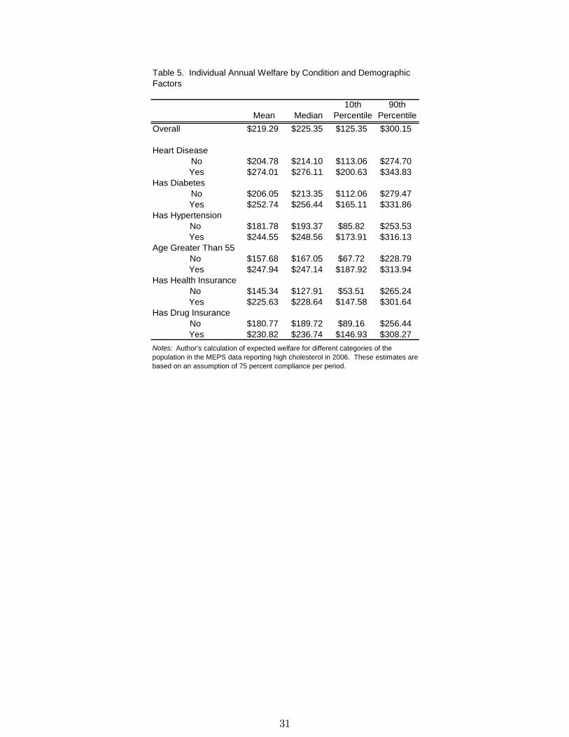
To highlight the importance of individual characteristics when conducting welfare analysis, Table
5 shows expected welfare for individuals with di¤erent types of health conditions and demographics
for 2006. The �rst row shows the welfare distribution for the entire population. The mean expected
welfare per year is $219, but there is a wide range in consumer welfare per individual with the
individuals at the 10th percentile valuing the drugs at $125 and those at the 90th percentile valuing
the drugs at $300. In general, Table 5 shows that those with more serious risk factors (i.e. heart
disease, diabetes, hypertension, and age over 55) tend to value these drugs more. Financial factors
also have a large impact on the value of these drugs. Both those with drug insurance and those
with health insurance value anti-cholesterol drugs more than those without insurance. The average
di¤erence in valuation for someone with health insurance compared to someone without health
insurance is around $81, about the same e¤ect as a serious risk factor, such as hypertension or
heart disease. To summarize, Table 5 shows that individual health and demographic variables
may have a large e¤ect on consumer welfare, which demonstrates the importance of including this
detailed individual information in the analysis.
[Table 5. Individual Annual Welfare by Condition and Demographic Factors]
This section has used the demand estimates to look at welfare levels in the market, the next
section examines how welfare changes over time may be translated into quality-adjusted prices.
5.1 Quality-Adjusted Prices
The demand estimates above are used to construct a quality-adjusted price index. Figure 3 shows
the quality-adjusted price compared to two benchmark price indexes: the average price and the
hedonic price. While the average price increases by almost 37 percent from 1996 to 2005, the
price index based on the demand estimates fell by 9 percent. The hedonic index is much closer to
the quality-adjusted price index and increases by only 4 percent over this period, con�rming the
important role of quality in the determination of price in this market. There are clear di¤erences
across these indexes pre-2005, but post-2005 all three indexes show a large decrease in price after
31Welfare �gures assume 75 percent compliance, which is discussed in greater detail in the appendix. Although it
is tempting to interpret these �gures, it may be di¢ cult to isolate particular factors a¤ecting welfare without further
analysis (i.e. the introduction of new products, price changes, generic entry, or changing health of the population
using anti-cholesterol drugs).
18

the introduction of the generic versions of Zocor and Pravachol.
[Figure 3. Price Index Comparison]
Several assumptions were made in constructing the quality-adjusted price index shown in Figure
3. To explore the importance of these assumptions, Table 6 presents alternative quality-adjusted
price indexes along with the average price, the hedonic price, and an additional benchmark price,
the Laspeyres index. The Laspeyres index uses prior period expenditures to weigh price changes,
similar to how price indexes are currently constructed at the BLS. The following are the di¤erent
assumptions made for the four di¤erent quality-adjusted price indexes reported in Table 6: (1)
ignores moral hazard issues caused by private drug insurance and allows the trend variable and
unobserved product characteristic, �jt, to vary over time; (2) controls for moral hazard issues by
removing the e¤ects of drug insurance, but allows the trend variable and unobserved product char-
acteristic to vary over time (the result reported in Figure 4 above); (3) removes drug insurance
e¤ects and �xes the trend variable to its initial value, but allows the unobserved product charac-
teristic to vary over time; (4) removes drug insurance e¤ects, �xes the trend variable to its initial
value, and the unobserved product characteristic is held constant over time. The results show some
variation among the price indexes, but the di¤erences appear relatively minor when compared to
the e¤ect of not correctly measuring the value of new goods. The quality-adjusted prices are all 13
to 18 percentage points lower than the Laspeyres price index by 2005.
[Table 6. Price Index Comparison and Alternative Assumptions (adjusted to 2007 $ using CPI)]
Each of the four indexes di¤er substantially from the average price, but the large price reduction
observed in 1997 using index (4) is quite di¤erent from indexes (1), (2), and (3) that each show a
small price increase followed by a gradual price decline. The reason for this di¤erence is that index
(4) �xes the value of �jt over time, which implies that a drug like Lipitor, that acquires greater
share in later years, may have a larger initial e¤ect on the quality-adjusted price index. Although
this initial di¤erence is interesting, index (4) moves closer to indexes (1) through (3) over time and
remains much lower than the average price over the entire period.
The quality-adjusted price indexes all show a substantial decline in the real price of anti-
cholesterol drugs, regardless of whether demand changes due to trends or whether unobserved mean
utility (�jt) is allowed to vary. This �nding contrast with results in Nevo (2003) who �nds that
quality-adjusted price indexes vary greatly for breakfast cereals depending on these assumptions.
A critical di¤erence between Nevo�s analysis and the market studied here is that unlike breakfast
19
cereals, where innovations are relatively small, the innovations in prescription drug markets may
be substantial. In particular, the innovations are large enough that alternative assumptions do not
a¤ect the basic result of declining prices for anti-cholesterol drugs. Therefore, while policy-makers
should remain cautious in applying market demand estimates to construct quality-adjusted prices
for a broad range of products, it may be useful to take this approach for constructing price indexes
in innovative markets, such as prescription drugs, where accounting for quality changes is likely to
be critical for obtaining meaningful price measures.
The quality-adjusted prices reported in Table 6 rely heavily on the estimates of the price coef-
�cient, �, which weighs the importance of price and the quality of the various products. To check
the sensitivity of the results presented here, Table A6 in the appendix shows the reported price
indexes for di¤erent values of �, ranging from the 5th percentile (� = �2:40) to the 95 percentile
(� = �:82). The results show that over this range of values the quality-adjusted price remains
about 15 to 28 percentage points below the Laspeyres index in 2005.
Although several new product introductions occur during the period of study that a¤ect quality-
adjusted prices, the primary innovation in this market �the introduction of statin drugs �occurred
prior to 1996. To show the importance of statin drugs at the beginning of the sample, welfare
estimates from the availability of statin drugs are calculated for 1996, the initial year of the sample.
Comparing consumer welfare estimates when statins are available to counterfactual welfare estimates
when statins are not available, I �nd that statin drugs accounted for 72 percent of consumer welfare
in 1996.32 Therefore, capturing quality-adjusted price declines from 1996 to 2007 may greatly
understate the true quality-adjusted price decline that may be observed over a longer horizon.
6 Conclusion
The impact of innovation on welfare is measured using a price index that holds the quality of anti-
cholesterol drug treatments �xed over time. The quality-adjusted price index is based on welfare
measures constructed from market demand estimates. This price index fell by 9 percent from 1996
to 2005, which contrasts sharply with the average price that increased by 37 percent and also di¤ers
from the Laspeyres index that grew by 9 percent. Thus, accounting for changes in quality appears
32A more detailed analysis of the welfare gains from the introduction of statin drugs is reported in Table A9 of the
appendix.
20

to be very important for properly measuring prices in the market for anti-cholesterol drugs. This
result highlights the potential importance of accounting for quality changes when measuring prices
and output in the health sector where technology is a primary driver of expenditure growth.
The demand model used to calculate a quality-adjusted price index in this paper re�ects the
market�s willingness-to-pay for prescription drugs. While this appears to provide a reasonable and
useful approximation to the value of anti-cholesterol drugs over time, it is possible that frictions in
the physician-insurer-patient relationship may cause the market�s willingness-to-pay for a drug to
not re�ect the patient�s preferences. For example, over-valuation of new technologies by physicians
would lead to an over-estimation in the welfare growth from the introduction of new drugs. Evidence
of the important role of physicians in the decision making process has been documented in the
literature with the work by Hellerstein (1998) who shows that the likelihood of prescribing generics
is largely determined by the physician and not the patient�s characteristics. More recently, Iizuka
(2007) looking at the Japanese market for anti-hypertensive drugs shows that physicians in Japan,
who also dispense prescription drugs, may select a prescription for a patient based on both the
patient�s preferences, but also their own pro�t motivation. More work needs to be done to study
the value of new technologies for patients when there are potential agency problems with physicians
or insurers.
One alternative approach for valuing new medical technology is to compare health expenditures
with health outcomes (see Cutler et al. (1998), Cutler and McClellan (2001), and Berndt et al.
(2002)), which does not rely on the physician-patient relationship. In particular, it may be inter-
esting to examine whether there are di¤erences in the value of new technologies based on health
outcomes compared to the predicted value of technologies based on market preferences.33 Another
approach for measuring the patient�s value of new technologies is to model the decisions and incen-
tives of the various agents (i.e. patients, insurers, and physicians), which would require signi�cantly
more information than is available from known data sources.33Although the two approaches are similar in their objective to measure the value of new technologies, they actually
answer distinct questions that provide di¤erent insight into the value of new goods. The market-based approach
is a re�ection of the market�s valuation of a product, while the outcomes based approach attempts to objectively
measure the welfare from medical treatments based on cost-e¤ectiveness studies that compare health outcomes and
the cost of inputs.
21

References
[1] Aizcorbe, Ana, and Nicole Nestoriak, (2010), �Price Indexes for Drugs: A Review of the Issues�,
Manuscript.
[2] Berry, Steven, James Levinsohn, and Ariel Pakes, (1993), �Estimating Discrete Choice Models
of Product Di¤erentiation�, RAND Journal of Economics, 25 pgs 242-262.
[3] Berry, Steven, (1994), �Estimating Discrete-Choice Models of Product Di¤erentiation�, RAND
Journal of Economics, 25(2) pgs 242-262.
[4] Berry, Steven, James Levinsohn, and Ariel Pakes, (1995), �Automobile Prices in Market Equi-
librium�, Econometrica, 63(4) pgs 841-890.
[5] Berry, Steven, James Levinsohn, and Ariel Pakes, (2004), �Di¤erentiated Products Demand
Systems from a Combination of Micro and Macro Data: The New Car Market�, Journal of
Political Economy 112(1) pgs 68-105.
[6] Berndt, Ernst, Anupa Bir, Susan H. Busch, Richard Frank, Sharon-Lise T. Normand, (2002),
�The Medical Treatment of Depression, 1991-1996: Productive Ine¢ ciency, Expected Outcome
Variations, and Price Indexes�, Journal of Health Economics, 21(3) pgs 373-396.
[7] Bresnahan, Timothy and Robert Gordon, (1997), �The Economics of New Goods�, NBER
Book Series Studies in Income and Wealth.
[8] Chintagunta, Pradeep, Jean-Pierre Dube, and Kim Yong Goh, (2005), �Beyond the Endogene-
ity Bias : The E¤ect of Unmeasured Brand Characteristics on Household-level Brand Choice
Models�, Management Science, 51(5), pgs 832-849.
[9] Cleanthous, Paris, (2004), �Patient Welfare Implications of Innovation in the U.S. Antidepres-
sant Market�, Working Paper.
[10] Cutler, David, (1995), �Technology, Health Costs, and the NIH�, National Institutes of Health
Roundtable on the Economics of Biomedical Research.
[11] Cutler, David, Mark McClellan, Joseph Newhouse, and Dalia Remler, (1998), �Are Medical
Prices Declining? Evidence From Heart Attack Treatments�, Quarterly Journal of Economics,
63(4) pgs 691-1024.
22

[12] Culter, David and Mark McClellan, (2001), �Is Technological Change in Medicine Worth It?�,
Health A¤airs, 20(5) pgs 11-29.
[13] Congressional Budget O¢ ce, (2008), �Technological Change and the Growth of Health Care
Spending�, The Congress of the United States, Congressional Budget O¢ ce. January.
[14] Gaynor, Martin and William Vogt, (2003), �Competition Among Hospitals�, RAND Journal
of Economics, 34(4) pgs 764-785.
[15] Goolsbee, Austan, and Amil Petrin, (2004), �The Consumer Gains from Direct Broadcast
Satellites and the Competition with Cable TV�, Econometrica, 72(2) pgs 351-381.
[16] Greenstein, Shane, (1996), �From Superminis to Supercomputers: Estimating Surplus in the
Computing Market�, The Economics of New Goods, University of Chicago Press, Chapter 8
pgs 329-372.
[17] Heart Protection Study Collaborative Group, (2010), �Statin Cost-E¤ectiveness in the United
States for People at Di¤erent Vascular Risk Levels�, Circulation: Cardiovascular Quality and
Outcomes, 2 pgs 65-72.
[18] Lucarelli, Claudio and Sean Nicholson, (2009), �A Quality-Adjusted Price Index for Colorectal
Cancer Drugs�, NBER Working Paper Series, Working Paper 15174.
[19] Mcfadden, D., (1981) �Econometric Models of Probabilistic Choice,� in C. Manski and D.
McFadden, Structural Analysis of Discrete Data, Cambridge, MA: The MIT Press.
[20] National Cholesterol Education Program, (2001), �Detection, Evaluation, and Treatment of
High Blood Cholesterol in Adults (Adult Treatment Panel III)�, National Institutes of Health,
National Heart, Lung, and Blood Institute.
[21] Newhouse, Joseph, (1992), �Medical Care Costs: How Much Welfare Loss?�, Journal of
Economic Perspectives, 6(3) pgs 3-21.
[22] Nevo, Aviv, (2003), �New Products, Quality Changes, and Welfare Measures Computed from
Estimated Demand Systems� The Review of Economics and Statistics, 85(2) pgs 266-275.
23

[23] Pakes, Ariel, Steven Berry, and James Levinsohn, (1993), �Applications and Limitations
of Some Recent Advances in Empirical I.O.: Price Indexes and Analysis of Environmental
Change.�American Economic Review, 83(2) pgs 240-46.
[24] Petrin, Amil, (2002), �Quantifying the Bene�ts of New Products: The Case of the Minivan�,
Journal of Political Economy, 110(4) pgs 705-729.
[25] Romeo, Charles, (2010), �Filling Out the Instrument Set in Mixed Logit Demand Systems for
Aggregate Data�, U.S. Department of Justice, Working Paper.
[26] Scandinavian Simvastatin Survival Group, (1994), �Randomized Trial of Cholesterol Lowering
in 4,444 Patients with Coronary Heart Disase: the Scandanavian SimvaStatin Survival Study
(4S)�, Lancet, 344 pgs 1383-9.
[27] Smith, Sheila, Stephen He er and Mark Freeland, (2000), �The Impact of Technological
Change on Health Care Cost Increases�, Working Paper.
[28] Smith, Sheila, Joseph Newhouse, and Mark Freeland, (2009), �Income, Insurance, and Tech-
nology: Why Does Health Spending Outpace Economic Growth�, Health A¤airs, 28(5) pgs
1276-84.
[29] Trajtenberg, Manuel, (1989), �The Welfare Analysis of Product Innovations, with an Applica-
tion to Computed Tomography Scanners�, Journal of Political Economy, 97(2) pgs 444-479.
[30] Trajtenberg, Manuel, (1990), �Product Innovation, Price Indices, and the (Mis)Measurement
of Economic Performance�, National Bureau of Economic Research, Working Paper No. 3261.
[31] Villas-Boas, J. and Russell Winer, (1999), �Endogneity in Brand Choice Models�,Management
Science, 45 pgs 1324-1338.
[32] Ward, S., M. Lloyd Jones, A Pandor, M Holmes, R Ara, A Ryan, W Yeo, and N Payne, (2007),
�A Systematic Review and Economic Evaluation of Statins for the Prevention of Coronary
Events�, Health Technology Assessment, 11(14).
[33] World Health Organization, (2002), �World Health Report 2002: Reducing Risks, Promoting
Healthy Life�, Geneva.
24

7 Tables
Figure 1. The Fraction of Individuals with HighCholesterol Over 20 that Use an AntiCholesterol Drug
60.0%
65.0%
70.0%
75.0%
80.0%
85.0%
90.0%
1996 1997 1998 1999 2000 2001 2002 2003 2004 2005 2006 2007
Source: Author's calculations using MEPS data for those individuals reporting high cholesterol.
25

Table 1. Market Share of Users of Anticholesterol Drugs
Drug Name Chemical 1996 1997 1998 1999 2000 2001 2002 2003 2004 2005 2006 2007Lipitor Atorvastatin Calcium 11.8% 28.2% 34.6% 39.1% 44.3% 44.2% 45.2% 43.5% 42.0% 38.4% 32.2%Zocor Simvastatin 27.2% 28.1% 24.8% 25.6% 24.9% 26.2% 26.7% 25.1% 23.4% 21.7% 13.0% 4.4%
Generic Zocor Simvastatin 8.1% 21.5%Pravachol Pravastatin Sodium 21.8% 18.3% 17.1% 15.6% 12.8% 11.5% 11.5% 9.9% 8.2% 6.3% 3.4% 1.6%
Generic Pravachol Pravastatin Sodium 1.2% 3.3%Mevacor Lovastatin 18.2% 12.6% 7.1% 5.1% 4.8% 2.7% 0.5% 1.3% 0.9% 0.3% 0.5% 0.6%
Generic Mevacor Lovastatin 4.2% 4.3% 5.3% 8.1% 9.1% 9.3%Crestor Rosuvastatin Calcium 0.4% 4.4% 4.6% 6.4% 6.9%Baycol Cerivastatin Sodium 1.3% 3.0% 4.7% 4.6%Vytorin Ezetimibe/Simvastatin 0.4% 4.3% 7.6% 8.5%Lescol Fluvastatin Sodium 11.6% 12.1% 9.3% 5.7% 4.1% 3.5% 4.2% 3.6% 2.5% 2.2% 2.1% 1.2%Advicor Lovastatin/Niacin 0.1% 0.4% 0.6% 0.6% 0.3% 0.3%
Nonstatins 21.3% 17.1% 12.3% 10.5% 9.7% 7.2% 8.5% 9.8% 10.7% 9.9% 9.9% 10.2%Source: Author's calculations using MEPS data. The unit of observation is the share of users of anticholesterol drugs. Baycol voluntarily withdrew in August of 2001because it was linked to over 31 deaths caused by muscle cell damage.
26
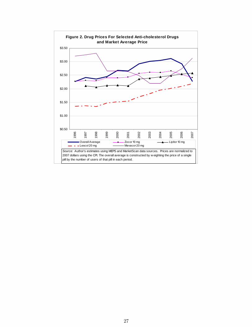
Figure 2. Drug Prices For Selected Anticholesterol Drugsand Market Average Price
$0.50
$1.00
$1.50
$2.00
$2.50
$3.00
$3.50
1996
1997
1998
1999
2000
2001
2002
2003
2004
2005
2006
2007
Overall Average Zocor 10 mg Lipitor 10 mgLescol 20 mg Mevacor 20 mg
Source: Author's estimates using MEPS and MarketScan data sources. Prices are normalized to2007 dollars using the CPI. The overall average is constructed by w eighting the price of a singlepill by the number of users of that pill in each period.
27

Table 2. Summary Statistics: Demographics
Variable Mean25th
Percentile50th
Percentile75th
percentile
Health Related DemographicsAge 62.08 52 63 74
Health Index 0.47 0.20 0.58 0.67Male 0.48
Has High Cholestorol 0.68Has Heart Disease 0.48
Has Diabetes 0.25Has Hypertension 0.53
Perceived Health is Good 0.10
Other DemographicsFamily Income (in 2007 $s) $54,591 $18,663 $40,123 $74,755
Number of Years of Education 11.87 10 12 14Drug Insurance 0.74
Health Insurance 0.96Medicare 0.52Medicaid 0.16
Number of Observations 106,510Source: Author's calculations using MEPS data.
28

Table 3. FirstStage Results from Conditional Logit Estimation
Variable Coef. zstatPrice*Risk Score 0.192 (3.3)
Price*Drug Insurance 0.045 (2.61)Price*Income 0.015 (2.21)
Drug Insurance 0.201 (3.65)Health Insurance 0.491 (7.42)
Log(Household Income/1000+1) 0.006 (0.27)High Cholesterol 4.354 (10.05)Heart Disease 0.813 (10.98)
Age 0.121 (3.47)Age^2 0.001 (1.68)Age^3 0.000 (5.05)
Age>=40 0.413 (4.16)Age*Male 0.011 (5.41)
Perceived Good Health 0.305 (7.58)Risk Score 2.013 (1.7)Education 0.020 (4.95)
Medicare Health Insurance 0.052 (1.31)Medicaid Health Insurance 0.069 (1.78)
Male 1.107 (7.13)Hypertension 0.457 (9.77)
Diabetes 0.465 (9.24)Log(Age Molecule) 0.699 (7.66)
Age*log(Age Molecule) 0.012 (7.88)Risk Score*log(Age Molecule) 0.173 (1.61)
Trend 0.132 (5.99)Risk Score*Trend 0.157 (7.35)
Number of ObservationsPseudo R2
Notes: Reported Zstatistics are based on robust standard errors clusteredby individual. Additional estimates of molecule drug interactions reported inthe appendix. Each variable reported here is relative to the nodrugtreatment option that has a utility normalized to zero.
106,5100.444
29

Table 4. SecondStage Demand Estimation
Variable Coef. zstat Coef. zstatPrice 1.613 (4.01) 0.107 (0.67)
Lipitor 20mg 0.878 (1.42) 0.817 (1.94)Lipitor 40mg 0.461 (0.66) 1.611 (3.65)Baycol .3mg 3.745 (5.38) 2.711 (4.57)Baycol .4mg 3.753 (4.7) 2.777 (3.99)
Cholestrimine 5.435 (8.37) 3.549 (8.36)Vytorin 20mg 2.015 (3.3) 2.797 (5.28)Vytorin 40mg 1.972 (3.24) 2.743 (5.18)
Zetia 2.371 (4.34) 2.864 (5.9)Fenofibrate 0.675 (1.53) 1.064 (2.71)
Lescol 20mg 4.475 (9.39) 3.563 (9.23)Lescol 40mg 3.931 (8.36) 3.070 (7.98)Generic Lopid 3.050 (3.51) 0.186 (0.38)
Lopid 3.112 (6.48) 2.175 (5.62)Advicor 2.346 (4.71) 2.322 (5.11)
Generic Mevacor 20mg 4.447 (5.63) 2.149 (4.17)Generic Mevacor 40mg 4.130 (6.31) 2.542 (5.24)
Mevacor 20mg 2.377 (5.31) 3.050 (8.02)Mevacor 40mg 1.505 (2.09) 3.715 (8.41)
Generic Niaspan 6.437 (6.75) 3.210 (6.32)Niaspan 5.029 (7.77) 3.182 (7.41)
Generic Pravachol 20mg 5.933 (6.45) 3.961 (5.51)Generic Pravachol 40mg 4.937 (5.62) 3.249 (4.57)
Pravachol 20mg 1.585 (3.86) 1.649 (4.41)Pravachol 40mg 0.699 (1.35) 1.898 (4.81)
Crestor 10mg 1.388 (2.47) 2.086 (4.27)Crestor 20mg 2.524 (4.5) 3.213 (6.58)
Generic Zocor 10mg 5.346 (6.11) 3.687 (5.19)Generic Zocor 20mg 2.888 (3.76) 2.353 (3.41)Generic Zocor 40mg 2.166 (2.82) 1.644 (2.38)
Zocor 10mg 1.596 (3.85) 1.831 (4.89)Zocor 20mg 1.659 (1.85) 1.319 (2.69)Zocor 40mg 1.121 (1.33) 1.627 (3.43)
Constant 12.901 (13.27) 16.368 (35.77)
Number of ObservationsR2
Notes: This Table shows estimates of mean utility on price, which are basedon the 266 productyear observations. The instruments used in the IVspecification are discussed in greater detail in the text. The 10 mg strength ofLipitor is the excluded dummy variable.
0.4566 0.606
OLSIV Estimation
266266
30
Mean Median10th
Percentile90th
PercentileOverall $219.29 $225.35 $125.35 $300.15
Heart DiseaseNo $204.78 $214.10 $113.06 $274.70Yes $274.01 $276.11 $200.63 $343.83
Has DiabetesNo $206.05 $213.35 $112.06 $279.47Yes $252.74 $256.44 $165.11 $331.86
Has HypertensionNo $181.78 $193.37 $85.82 $253.53Yes $244.55 $248.56 $173.91 $316.13
Age Greater Than 55No $157.68 $167.05 $67.72 $228.79Yes $247.94 $247.14 $187.92 $313.94
Has Health InsuranceNo $145.34 $127.91 $53.51 $265.24Yes $225.63 $228.64 $147.58 $301.64
Has Drug InsuranceNo $180.77 $189.72 $89.16 $256.44Yes $230.82 $236.74 $146.93 $308.27
Table 5. Individual Annual Welfare by Condition and DemographicFactors
Notes: Author's calculation of expected welfare for different categories of thepopulation in the MEPS data reporting high cholesterol in 2006. These estimates arebased on an assumption of 75 percent compliance per period.
31

Figure 3. Price Index Comparison
0.5
0.6
0.7
0.8
0.9
1
1.1
1.2
1.3
1.4
1.5
1996 1997 1998 1999 2000 2001 2002 2003 2004 2005 2006 2007
Notes: The qualityadjusted price index is calculated as described in the text. Prices are normalized to2007 dollars using the CPI. The hedonic regression estimate used to calculate the hedonic price index isreported in the appendix.
Avg Price Hedonic QualAdj
32

Year Avg Price Laspeyres Hedonic (1) (2) (3) (4)1996 1.00 1.00 1.00 1.00 1.00 1.00 1.001997 1.07 0.99 0.99 1.03 1.03 1.04 0.871998 1.04 0.98 0.92 1.03 1.03 1.05 0.851999 1.08 1.01 0.94 0.94 0.95 0.97 0.872000 1.18 1.01 0.96 0.93 0.93 0.96 0.872001 1.17 1.00 0.95 0.90 0.90 0.93 0.872002 1.29 1.04 1.01 0.91 0.92 0.95 0.912003 1.33 1.07 1.04 0.90 0.90 0.94 0.892004 1.34 1.07 1.04 0.89 0.90 0.93 0.892005 1.37 1.09 1.04 0.91 0.91 0.96 0.912006 1.29 1.08 0.98 0.89 0.90 0.95 0.912007 1.00 0.88 0.67 0.74 0.73 0.77 0.74
WithInsurance
RemovingInsurance
RemovingInsurance
RemovingInsurance
With Trend With Trend No Trend No TrendWith Error With Error With Error No Error
QualityAdjusted Price Indexes
Table 6. Price Index Comparison Under Alternative Assumptions
Notes: The qualityadjusted price index is calculated as described in the text. These figures areadjusted to 2007 dollars using the CPI. The hedonic regression estimate used to calculate the hedonicprice index is reported in the appendix. The Laspeyres index follows the BLS methodology wheregenerics and Branded versions of the same molecule are treated as an identical product and the priceindex is computed using a geometric mean.
33