Forschungsinstitut zur Zukunft der ArbeitInstitute for the Study of Labor

DI

SC

US

SI

ON

P

AP

ER

S

ER

IE

S

Drought of Opportunities:Contemporaneous and Long-Term Impacts ofRainfall Shocks on Human Capital

IZA DP No. 9440

October 2015

Manisha ShahBryce Millett Steinberg

Drought of Opportunities:

Contemporaneous and Long-Term Impacts of Rainfall Shocks on Human Capital

Manisha Shah University of California, Los Angeles,

NBER and IZA

Bryce Millett Steinberg

Harvard University

Discussion Paper No. 9440 October 2015

IZA

P.O. Box 7240 53072 Bonn

Germany

Phone: +49-228-3894-0 Fax: +49-228-3894-180

E-mail: iza@iza.org

Any opinions expressed here are those of the author(s) and not those of IZA. Research published in this series may include views on policy, but the institute itself takes no institutional policy positions. The IZA research network is committed to the IZA Guiding Principles of Research Integrity. The Institute for the Study of Labor (IZA) in Bonn is a local and virtual international research center and a place of communication between science, politics and business. IZA is an independent nonprofit organization supported by Deutsche Post Foundation. The center is associated with the University of Bonn and offers a stimulating research environment through its international network, workshops and conferences, data service, project support, research visits and doctoral program. IZA engages in (i) original and internationally competitive research in all fields of labor economics, (ii) development of policy concepts, and (iii) dissemination of research results and concepts to the interested public. IZA Discussion Papers often represent preliminary work and are circulated to encourage discussion. Citation of such a paper should account for its provisional character. A revised version may be available directly from the author.

IZA Discussion Paper No. 9440 October 2015

ABSTRACT

Drought of Opportunities: Contemporaneous and Long-Term Impacts of Rainfall Shocks on Human Capital*

Higher wages are generally thought to increase human capital production, particularly in the developing world. We introduce a simple model of human capital production in which investments and time allocation differ by age. Using data on test scores and schooling from rural India, we show that higher wages increase human capital investment in early life (in utero to age 2) but decrease human capital from ages 5-16. Positive rainfall shocks increase wages by 2% and decrease math test scores by 2-5% of a standard deviation, school attendance by 2 percentage points, and the probability that a child is enrolled in school by 1 percentage point. These results are long-lasting; adults complete 0.2 fewer total years of schooling for each year of exposure to a positive rainfall shock from ages 11-13. We show that children are switching out of school enrollment into productive work when rainfall is higher. These results suggest that the opportunity cost of schooling, even for fairly young children, is an important factor in determining overall human capital investment. JEL Classification: O12, I2, J1 Keywords: human capital investment Corresponding author: Manisha Shah Department of Public Policy University of California, Los Angeles Los Angeles, CA 90095 USA E-mail: ManishaShah@ucla.edu

* We would like to thank Marianne Bitler, Kitt Carpenter, Thomas Covert, Joe Cummins, James Feigenbaum, Ed Glaeser, Ben Hebert, Simon Jaeger, Rob Jensen, Marc Jeuland, Larry Katz, Michael Kremer, Xiaoman Luo, Emily Oster, Guillaume Pouliot, Martin Rotemberg, Jesse Shapiro, Ashish Shenoy, and Chad Stecher for helpful comments. Seminar participants at CMC, CSUF, Harvard, HKUST, NBER Summer Institute, UC Berkeley, UCI, UCSC, USC, and PacDev provided useful feedback. We thank Wilima Wadhwa for generously sharing the ASER data.

1 Introduction

Human capital investment is an important determinant of economic growth (Mankiw et al.,

1992). The majority of empirical evidence from poor countries suggests that higher wages

should increase human capital investment (see for example, Jacoby and Skoufias (1997);

Jensen (2000); Thomas et al. (2004); Maccini and Yang (2009)). However, there is some

evidence from Latin America suggesting the opposite (Duryea and Arends-Kuenning, 2003;

Schady, 2004; Kruger, 2007).1 Theoretically, the relationship is ambiguous; if time and

income are important inputs into human capital, then increased wages could either increase

or decrease human capital investment. As early as 1977, Rosenzweig and Evenson showed

that higher wages are associated with lower schooling rates, due to increased opportunity

costs of staying in school. If poor children react to higher wages by leaving school early to

join the workforce, this could raise overall inequality in poor countries or even stunt long

term growth.

Some of the differences in these studies may be due to differential effects by age. If

the opportunity cost of time for older children is affected by wages, then the substitution

effect would be relatively important for older children. In addition, if the human capital

production function itself differs by age (for instance, if income-intensive inputs such as

calories are more important for younger children), then we might also observe differential

impacts of wage shocks by age.

In this paper, we introduce a simple model of human capital investment in which house-

holds derive utility from consumption and human capital. We then estimate the comparative

statics from this model, using rainfall fluctuations in rural India as quasi-random shocks to

wages. We measure human capital using test scores from the ASER data from 2005-2009;

we observe approximately 2 million rural children from almost every rural district in India.

The data includes four distinct measures of literacy and numeracy for each child whether

1All of these papers use school enrollment or years of schooling as their measure of human capital invest-ment.

1

or not he is currently enrolled in school.2 In addition, our data allow us to look at more

standard educational measures such as school enrollment, drop out behavior, and being on

track in school (age for grade). Since the survey is conducted every year over five years, we

can control for age, year of survey, and district, identifying off within-district variation in

rain shock exposure.

The estimates of the effect of school-aged wages on human capital suggest that going

from regular rainfall to a positive rainfall shock increases wages by 2% and decreases math

test scores by 2-5% of a standard deviation, decreases school attendance by 2 percentage

points, and decrease the probability that a child is enrolled in school by 1 percentage point.

This implies that a positive rainfall shock increases the urban-rural enrollment gap by 15%

for 5 to 16 year olds. In addition, children who experienced a positive rainfall shock in the

previous year are 5.5% more likely to have dropped out of school and 4.5% more likely to be

behind in school.

We also estimate the impacts of early life rainfall shocks (in utero to age 4) on current test

scores and schooling outcomes. We find that, by contrast, more early life rainfall is associated

with higher test scores in both math and reading. A positive rainfall shock increases wages

2% and increases current test scores for children who experienced a positive rainfall shock

in utero to age 2 by about 1.3% of a standard deviation per year of exposure. In addition,

children who experience positive rainfall shocks before age 5 are more likely to be enrolled

in school and to be on track in school.

We investigate whether there are long-term impacts of these rainfall shocks on total years

of schooling for adults aged 16-30 using a national labor and employment survey. We find

that more rainfall during school years (particularly ages 11-13) lowers total years of schooling.

This is also the age group where positive rainfall shocks significantly increase the likelihood of

dropping out as these are the transition years from primary to secondary school so positive

employment shocks are particulary detrimental to human capital investment during this

2This is rare since tests are primarily conducted at school, and thus scores are usually only available forcurrently enrolled kids who attended school on the day the test was given.

2

period.

As far as we know, this is the first paper to document the possibility that positive

productivity shocks can lead to lower levels of human capital attainment using test scores.

Test scores measure output as opposed to the previous literature which has focused on school

enrollment (i.e. inputs). Unlike the previous literature which focuses on shocks at certain

critical ages in a child’s development, we consider a child’s entire lifecycle from in utero to age

16. This allows us to say something about the relative importance of time vs. income at all

stages of a child’s human capital development. We show that wages increase human capital

investment from the in utero phase to age two, but decrease human capital investment after

age 5. In addition, we provide new evidence on the long term effects of cumulative shocks on

human capital attainment of young adults. While previous research has suggested that that

these shocks represent simple intertemporal substitution of school time and that children

make up these differences in human capital (Jacoby and Skoufias, 1997; Funkhouser, 1999),

we find quite the opposite. For example, children ages 11-13 complete approximately .2

more years for every drought experienced (and .2 fewer years for every positive rainfall shock

relative to normal rainfall years). This constitutes a substantial shock to human capital

attainment during a period when most poor children will already be on the margin between

dropping out and continuing.

2 A Model of Human Capital Investment

We consider a simple model of human capital investment. Households consist of one child

and one parent, and the parent maximizes the total utility of the household. The child lives

for three periods. In the first period, the child is too young for school or work and only

consumes. In the second period, the child also consumes, but in addition, she has one unit

of time that can be spent either in school or working. In the third period, the household

gets a payoff from the child’s accumulated human capital.

Let ct be consumption in period t where t ∈ {1, 2}, and ut(ct) be the flow utility from

3

consumption in period t, where ∂ut∂ct

> 0 and ∂2ut∂c2t

< 0, ∀t. Let et be the human capital of

the child in period t, and h be the human capital of the parent, which we assume does not

change. Let V (e3) be the payoff to the household from the level of human capital in period

3. β is the discount factor.3 The total utility function of the household is

U(c1, c2, e3) = u1(c1) + βu2(c2) + β2V (e3)

Let wt ∈ (0, w̄) denote the wage in period t per unit of human capital, so that parents will

be paid wth and children will be paid wtet for each unit of time spent working in period t.

wt can be thought of as an aggregate productivity shifter, and in our empirical specifications

will be proxied by rainfall in agricultural areas. The wage is determined exogenously. In

addition, let s2 ∈ [0, 1] denote the time that the child spends in school in period 2, and thus

(1 − s2) will be the time she spends working. In the first period, household income will be

earned entirely by the parent, and will be equal to his wage, w1h. In the second period, the

household income will be equal to the earnings of the parent, w2h plus the earnings of the

child, (1− s2)w2e2. We will abstract away from borrowing and savings decisions, so that

consumption will always be equal to income in each period. Thus, consumption will be

c1 = w1h

c2 = w2(h+ (1− s2)e2)

In the spirit of Cunha and Heckman (2007), we assume that human capital at date t is

a function of human capital at date t− 1 plus any investments made in period t− 1. In this

simple model, investments will take the form of either schooling or consumption. We will

not allow for directed payments for human capital (such as books or tutors) or for parents

to invest their own time to teach children. This is sensible in the context of rural India

3For ease of notation, we assume exponential discounting, even though in this model, the “periods” areof substantially different lengths. This has no effect on our results.

4

since primary school is free and compulsory,4 and the Indian government has built many

schools to keep the costs of attendance low.5 In addition, the parents of these children often

have very low human capital themselves, so it is unlikely that they are heavily involved in

teaching their children literacy or numeracy.

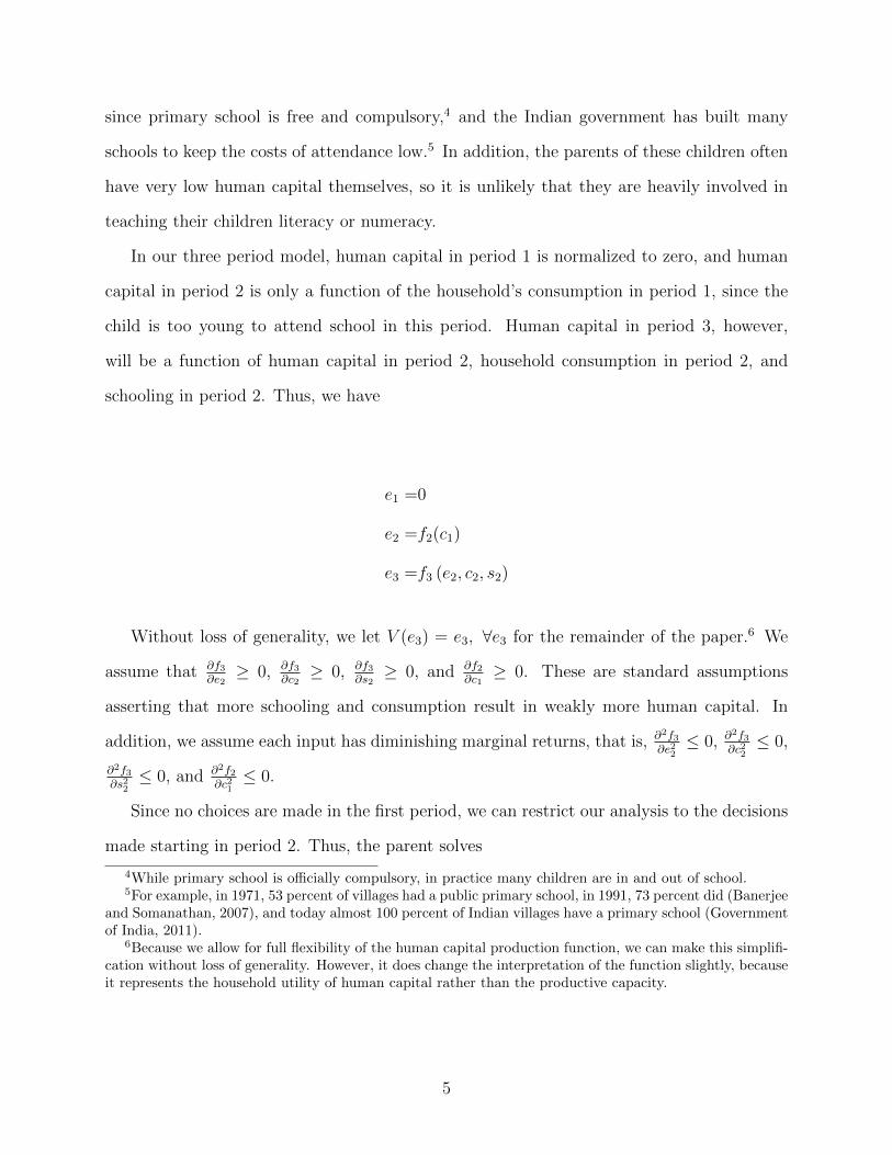
In our three period model, human capital in period 1 is normalized to zero, and human

capital in period 2 is only a function of the household’s consumption in period 1, since the

child is too young to attend school in this period. Human capital in period 3, however,

will be a function of human capital in period 2, household consumption in period 2, and

schooling in period 2. Thus, we have

e1 =0

e2 =f2(c1)

e3 =f3 (e2, c2, s2)

Without loss of generality, we let V (e3) = e3, ∀e3 for the remainder of the paper.6 We

assume that ∂f3∂e2≥ 0, ∂f3

∂c2≥ 0, ∂f3

∂s2≥ 0, and ∂f2

∂c1≥ 0. These are standard assumptions

asserting that more schooling and consumption result in weakly more human capital. In

addition, we assume each input has diminishing marginal returns, that is, ∂2f3∂e22≤ 0, ∂2f3

∂c22≤ 0,

∂2f3∂s22≤ 0, and ∂2f2

∂c21≤ 0.

Since no choices are made in the first period, we can restrict our analysis to the decisions

made starting in period 2. Thus, the parent solves

4While primary school is officially compulsory, in practice many children are in and out of school.5For example, in 1971, 53 percent of villages had a public primary school, in 1991, 73 percent did (Banerjee

and Somanathan, 2007), and today almost 100 percent of Indian villages have a primary school (Governmentof India, 2011).

6Because we allow for full flexibility of the human capital production function, we can make this simplifi-cation without loss of generality. However, it does change the interpretation of the function slightly, becauseit represents the household utility of human capital rather than the productive capacity.

5

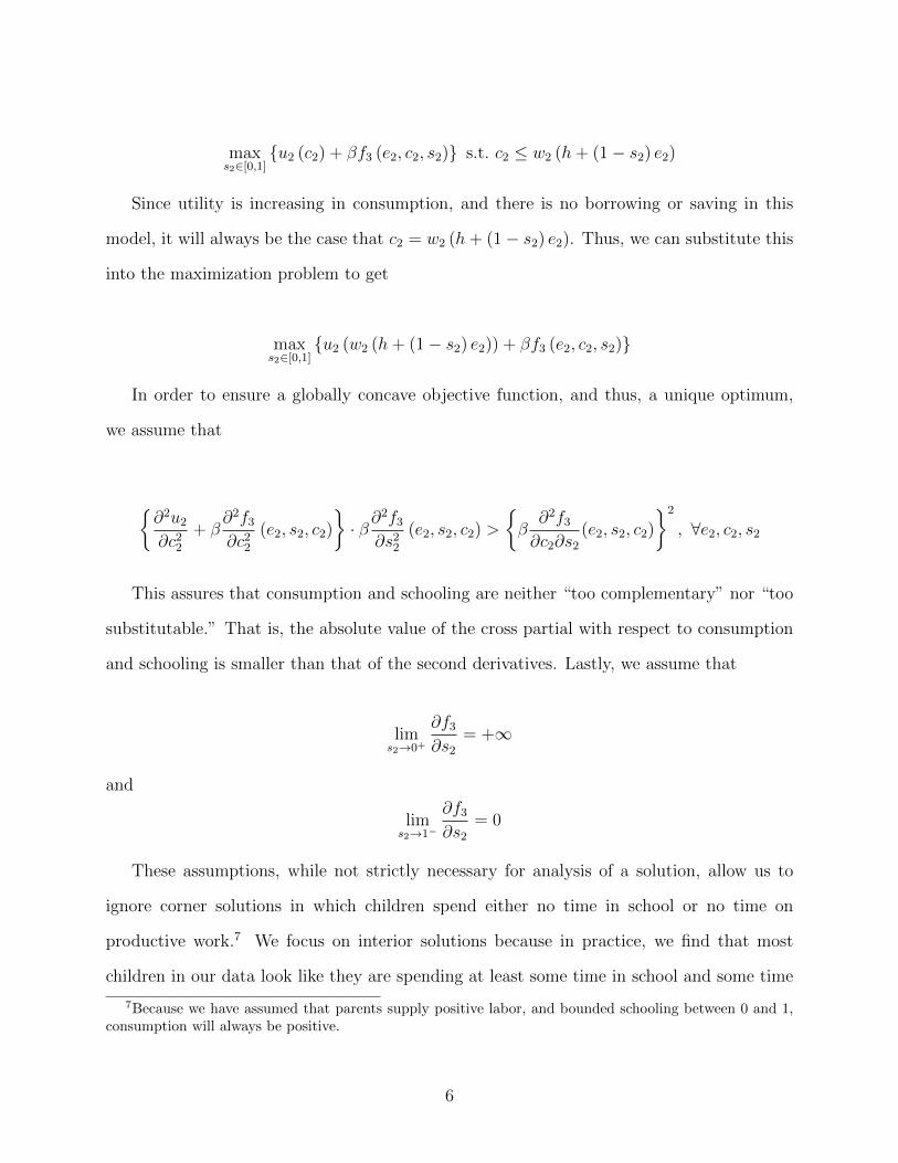
maxs2∈[0,1]

{u2 (c2) + βf3 (e2, c2, s2)} s.t. c2 ≤ w2 (h+ (1− s2) e2)

Since utility is increasing in consumption, and there is no borrowing or saving in this

model, it will always be the case that c2 = w2 (h+ (1− s2) e2). Thus, we can substitute this

into the maximization problem to get

maxs2∈[0,1]

{u2 (w2 (h+ (1− s2) e2)) + βf3 (e2, c2, s2)}

In order to ensure a globally concave objective function, and thus, a unique optimum,

we assume that

{∂2u2

∂c22

+ β∂2f3

∂c22

(e2, s2, c2)

}· β∂

2f3

∂s22

(e2, s2, c2) >

{β∂2f3

∂c2∂s2

(e2, s2, c2)

}2

, ∀e2, c2, s2

This assures that consumption and schooling are neither “too complementary” nor “too

substitutable.” That is, the absolute value of the cross partial with respect to consumption

and schooling is smaller than that of the second derivatives. Lastly, we assume that

lims2→0+

∂f3

∂s2

= +∞

and

lims2→1−

∂f3

∂s2

= 0

These assumptions, while not strictly necessary for analysis of a solution, allow us to

ignore corner solutions in which children spend either no time in school or no time on

productive work.7 We focus on interior solutions because in practice, we find that most

children in our data look like they are spending at least some time in school and some time

7Because we have assumed that parents supply positive labor, and bounded schooling between 0 and 1,consumption will always be positive.

6

on productive work.

At an interior optimum, parents equalize the marginal utility consumption from forgoing

school now with the marginal benefits of additional human capital later:

w2e2∂u2

∂c2

= βΘ(w2, e2, s∗2, c∗2)

where

Θ(w2, e2, s∗2, c∗2) =

∂f3

∂s2

(e2, s∗2, c∗2)− w2e2

∂f3

∂c2

(e2, s∗2, c∗2)

Households tradeoff the marginal benefit of additional utility from consumption with the

net long-term benefit of schooling. Note that in an interior solution, since ∂u2∂c2, w2, e2 > 0, it

must be the case that Θ(w2, e2, s∗2, c∗2) > 0. That is, at the optimum, schooling is a relatively

better technology than working and consuming for turning time into human capital.

We are interested in the effect that wages have on the optimal level of schooling. That

is, if wages increase, do children invest more or less in schooling? And, as a result, do overall

levels of human capital increase or decrease? In this model, there are two relevant wages—

those in early life and those during the child’s school years. We will examine the effect of

each of these wages on schooling choices and human capital.

2.1 Effect of School-Aged Wages on Schooling and Human Capital

First, we examine the impact of second period wages, w2 on the optimal choice of schooling,

s∗2, and the resulting level of human capital, e∗3. From the first order condition,

∂s∗2∂w2

∝ −

Substitution Effect (-)︷ ︸︸ ︷e2

(∂u2

∂c2

+ β∂f3

∂c2

)−

Income Effect (+)︷ ︸︸ ︷(h+ (1− s∗2) e2)w2e2

∂2u2

∂c22

+

Effect of c2 on Net Impact of Schooling︷ ︸︸ ︷(h+ (1− s∗2) e2) β

∂Θ

∂c2

(1)

The effect of school-aged wages on the optimal level of schooling will depend on three

things. First, increased wages increase the benefit to working, both through the utility

7

in period 2, and through the benefit to human capital in period 3 (substitution effect).

Second, increased wages will increase consumption, which will decrease the marginal utility of

consumption (income effect). Third, the increase in consumption could affect the net impact

of schooling. We think it is likely that this term is weakly positive. That is, as consumption

increases, schooling becomes relatively better than consumption as a technology for turning

time into human capital. If a child is starving, consumption is likely extremely important

for the production of human capital. As the level of consumption increases, the benefits

of consumption relative to schooling will likely decrease. Thus, even if income effects are

small, if schooling becomes relatively more valuable as households get richer, we could still

see schooling decrease when wages are higher. Which of these forces will dominate is an

empirical question that we address in Section 4.1.

We examine the impact of period 2 wages on period 3 human capital:

d

dw2

(f3 (e2, c∗2, s∗2)) = (h+ (1− s∗2)e2)

∂f3

∂c2

+ Θ∂s∗2∂w2

(2)

The first term in this expression is positive by assumption: it is the mechanical effect

of higher wages on consumption which in turn increases human capital. We also know that

Θ is positive at any interior optimum, so if increased wages lead to increased schooling, we

know that human capital will increase as a result. However, if increased wages decrease the

optimal level of schooling, then the effect on human capital will be ambiguous. The sign

will depend on whether this behavioral effect of lower investment will offset the mechanical

increase in human capital due to consumption.

2.2 Effect of Early Life Wages on Schooling and Human Capital

In this model, the only way that early life wages affect the choice of schooling is through

their effect on human capital in period 2. Because increased wages mechanically increase

consumption in period 1, and human capital in period 2 is an increasing function of period

8

1 consumption, increased wages in period 1 will always result in increased human capital in

period 2:

d

dw1

(e2) =∂f2

∂c1

∂c1

∂w1

= h∂f2

∂c1

> 0

Thus, in order to understand the effect of early life wages on schooling and later-life

human capital, it is sufficient to study the effect of period 2 human capital on the optimal

level of schooling and on period 3 human capital.

∂s∗2∂w1

= h∂f2

∂c1

∂s∗2∂e2

∝ ∂s∗2∂e2

From the first order condition, we can derive the effect of period 2 human capital on the

optimal choice of schooling:

∂s∗2∂e2

∝

Substitution Effect (-)︷ ︸︸ ︷−w2

∂u2

∂c2

Income Effect (+)︷ ︸︸ ︷−w2

2e2 (1− s∗2)∂2u2

∂c22

+β

Net impact of additional e2 on Θ︷ ︸︸ ︷[∂Θ

∂e2

+ w2 (1− s∗2)∂Θ

∂c2

](3)

Increased period 2 human capital has three effects on the optimal level of schooling.

First, increased human capital increases the value of work in the second period (substitution

effect). Second, increased human capital leads to higher income, which reduces the marginal

utility of consumption (income effect). Third, the net benefit of schooling, Θ(w2, e2, s∗2, c∗2),

could be affected by the increase in human capital, in two ways. First, if there are “dynamic

complementarities” in the sense of Cunha and Heckman (2007), we would expect the return

to schooling to increase with early life investments. In addition, since additional early life

human capital also increases consumption mechanically, this could also effect the net benefit

of schooling even without dynamic complementarities. However, whether these effects will

be large enough to overcome the substitution effects is again an empirical question, which

we will address in Section 4.2.

We can examine the impact of childhood human capital on adult human capital. Again,

9

e∗3 = f3 (e2, c∗2, s∗2)

d

de2

(e∗3) =∂f3

∂e2

+∂f3

∂c2

w2 (1− s∗2) + Θ∂s∗2∂e2

(4)

Intuitively, the first term can be thought of as the persistence of early life human capital,

and is weakly positive by assumption. The second term takes into account the mechanical in-

crease in consumption derived from an increase in early life human capital (through increased

wages) and is also positive by assumption. From the third term, we know that Θ is positive

at the optimum, so if early life human capital increases schooling, then it will unambiguously

increase human capital as well. If not, it is unclear which effect will dominate.

In the following sections, we will empirically estimate ∂c1∂w1

,∂s∗2∂w2

,∂s∗2∂w1

, ddw1

(e∗3), and ddw2

(e∗3).

3 Background and Data

3.1 Cognitive Testing and Schooling Data

Every year since 2005, the NGO Pratham has implemented the Annual Status of Education

Report (ASER), a survey on educational achievement of primary school children in India

which reaches every rural district in the country.8 We have data on children from 2005-

2009, giving us a sample size of approximately 2 million rural children. The sample is a

representative repeated cross section at the district level. The ASER data is unique in

that its sample is extremely large and includes both in and out of school children. Since

cognitive tests are usually administered in schools, data on test scores is necessarily limited

to the sample of children who are enrolled in school (and present when the test is given).

However, ASER tests children ages 5-16, who are currently enrolled, dropped out, or have

never enrolled in school. In Table 1 we describe the characteristics of the children in our

8This includes over 570 districts, 15,000 villages, 300,000 households and 700,000 children in a givenyear. For more information on ASER, see http://www.asercentre.org/ngo-education-india.php?p=

ASER+survey

10

sample as well as their test scores.

The ASER surveyors ask each child four questions each in math and reading (in their

native language). The four math questions are whether the child can recognize numbers

1-9, recognize numbers 10-99, subtract, and divide. The scores are coded as 1 if the child

correctly answers the question, and 0 otherwise. In 2006 and 2007, children were also asked

two subtraction word problems, which we use as a separate math score (Math word problem).

The four literacy questions are whether the child can recognize letters, recognize words, read

a paragraph, and read a story. We calculate a “math score” variable, which is the sum of the

scores of the four numeracy questions. For example, if a child correctly recognizes numbers

between 1-9 and 10-99, and correctly answers the subtraction question, but cannot correctly

answer the division question, then that child’s math score would be coded as 3. The “reading

score” variable is calculated in exactly the same way. In addition, the survey asks about

current enrollment status and grade in school, and in 2008, attendance in the past week.9

Table 1 summarizes the means of test scores and the schooling outcomes for children in the

ASER sample.

3.2 NSS Data

To examine the impact of rainfall shocks on work and wages, we use the NSS (National

Sample Survey) Rounds 60, 61, 62, and 64 of the NSS data which was collected between

2004 and 2008 by the Government of India’s Ministry of Statistics. This is a national labor

and employment survey collected at the household level all over India. This dataset gives us

measures of employment status as well as wages at the individual level. Given the potential

measurement error in the valuation of in-kind wages, we define wages paid in money terms.

We use data from all rural households in this survey and merge with our district level rainfall

data to explore the relationship between weather shocks, labor force participation, school

attendance, and wages.

9More information on the ASER survey questions, sampling, and procedures can be found in the ASERdata appendix.

11

3.3 Rainfall Data

We use monthly rainfall data which is collected by the University of Delaware to determine

rainfall shock years within districts.10 The data covers all of India in the period between

1900-2008 and we use data from 1975-2008 in this paper. The data is gridded by longitude

and latitude lines, so to match these to districts, we simply use the closest point on the grid

to the center of the district, and assign that level of rainfall to the district for each year.

We define a positive shock as yearly rainfall above the 80th percentile and negative shock

(drought) as rainfall below 20th percentile within the district. The “positive” and “negative”

shocks should not be taken in an absolute sense—we are not comparing districts that are

prone to higher rainfall to those that are prone to lower rainfall. These are simply high or

low rainfall years for each district within the given time frame. For the analysis, we define

“rain shock” as equal to 1 if rainfall is above the 80th percentile, -1 if rainfall is below the

20th percentile, and 0 otherwise. These are similar to the definitions employed in Kaur

(2011) and Jayachandran (2006).11 Table A2 shows the percent of districts each year that

experience a drought or positive rainfall shock; the variation in rainfall across time and space

is quite extensive.

In a data appendix, we explicitly test for serial correlation of rainfall because if droughts

this year are correlated with droughts next year, it is difficult to tell the extent to which

we are picking up the effects of a single shock or multiple years of rainfall shocks. However,

we find no significant evidence of serial correlation across years. In addition, we check for

spatial correlation. If there is significant within-district variation in rainfall, our district-level

measure of rainfall variation might be missing the true effects for many of the children in

our sample. However, we find that this type of very local variation is unlikely to be biasing

our results (results available upon request).

10The data is available at: http://climate.geog.udel.edu/~climate/html_pages/download.html#

P200911In previous versions of the paper we showed results separately for positive and negative rainfall shocks

and using rainfall quintiles and the results are qualitatively similar.

12

3.4 Rainfall Shocks in India

In rural India, 66.2 percent of males and 81.6 percent of females report agriculture (as

cultivators or laborers) as their principal economic activity (Mahajan and Gupta, 2011).

Almost 70 percent of the total net area sown in India is rainfed; thus, in this context we

would expect rainfall to be an important driver of productivity and wages. While there is

plenty of evidence showing droughts adversely affect agricultural output and productivity

in India (see for example Rao et al. (1988), Pathania (2007)), we also explore this question

empirically using the World Bank India Agriculture and Climate Data set. In Table A1 we

show results from regressions of rice, wheat, and jowar yields on rainfall shocks. In drought

years, crop yields are significantly lower regardless of the type of crop (and the opposite is

true in positive rain shock years).

In Table A1, we measure the effect of rainfall shocks on wages using NSS data.12 We

find that for positive rainfall shocks result in increased wages. In Table A1, we also show

that agricultural yields are significantly higher across all types of crops in years with more

rainfall, controlling for labor and other inputs. These results give us confidence that rainfall

shocks are indeed a productivity, and thus, wage shifter in this context.

4 Empirical Strategy and Results

In Section 2, we outlined a model in which the effects of early life and school-aged wages on

human capital was ambiguous. We now estimate these comparative statics using the test

score and schooling data from India.

To understand the impact of school-aged wages on schooling and human capital, we

estimate the impact of current year rainfall shocks on current levels of schooling and human

capital. To determine the effects of early life wages on human capital outcomes, we need to

regress current test scores on lagged rainfall since we do not have measures of human capital

12While there is extensive literature in economics and other fields both documenting this fact and usingit to estimate economic parameters of interest (see for example Jayachandran (2006); Maccini and Yang(2009); Jensen (2000); Kaur (2011)), we also test for the relationship using our data.

13

for very young children. In both cases, we will rely on the quasi-random nature of negative

and positive rainfall shocks within districts as a natural shifter of rural wages. We outline

both strategies in detail below.

4.1 Estimating Effect of School-Aged Wages on Schooling and Human Capital

In order to determine the impacts of wages on human capital and schooling (∂s∗2∂w2

and ddw2

(e∗3)),

we estimate the regression:

Sijty = α + β1δj,y + β2δj,y−1 + ζθj,t + γj + φt + ψy + εijty (5)

where Sijty is the measure of human capital or schooling for student i in district j born in

year t and surveyed in year y. As measures of e3, we use math and reading test scores, as well

as “on track” which is a measure of age-for-grade. We define on track as a binary variable

which indicates if a child is in the correct grade for his/her age. The variable is coded 1 if

age minus grade is at most six. That is, if an eight year old is in second or third grade, he is

coded as on track, but if he is in first grade, he is not. We use self-reported attendance and

an indicator of having dropped out of school as two measures of s2, schooling in period 2.

δj,y is rain shock in district j in year y and δj,y−1 is a lagged rain shock. β1 is the impact of

current year rain shock on the various cognitive test scores and schooling outcomes. We also

control for early life rainfall exposure by including θj,t, a vector of early life rainfall shocks

from in utero to age 4. γj is a vector of district fixed effects, φt is a vector of age fixed effects,

and ψy is a vector of year of survey fixed effects. This specification allows us to compare

children who are surveyed in different years from the same district. Since our regressions

contain district level fixed effects, the coefficient will not be biased by systematic differences

across districts. Standard errors are clustered at the district level.

In Panel A of Table 2 we report the results from Equation 5 estimating the impact of

contemporaneous rainfall shocks on test scores and schooling outcomes of children ages 5-

14

16.13 The coefficient on math score is -.02, which means that, relative to a positive rainfall

year, children tested in a drought year score .04 points better (or 1.5 percent) on the math

test. The coefficient on math word problem is -.05 which means that relative to a positive

rainfall year, children in a drought district score 0.1 points more (or 8 percent). While rain

shocks this year do not impact reading scores, positive rainfall shocks in the previous year

significantly decrease reading scores as well.

Rainfall shocks in the previous year significantly affect both age for grade and dropping

out. Children in a positive rainfall shock year are .4 percentage points more likely to report

having dropped out in the following year, relative to children tested in drought years (this is

an increase of 11% from a mean of .036). Likewise, children tested in a positive shock year are

2 percentage points less likely to be on track, relative to a drought year. In addition, children

who currently experience drought are 4 percentage points more likely to have attended school

in the previous week (from a mean of 86 percent) relative to a positive rainfall shock.

In Panels B and C of Table 2, we report these coefficients separately estimated for children

aged 5-10 and aged 11-16. Most of the magnitudes are similar in size, although the effect

of rainfall on dropouts and being on track appears to be almost entirely driven by older

children. Indeed, Figure 1 shows the the coefficient of lagged rain shock on dropping out

estimated for each age separately. It appears that experiencing a positive rainfall shock from

age 12 onward results in a higher likelihood of dropping out, though the estimates are noisy.

This makes sense since this is the period children transition from primary to secondary school

and when outside job opportunities during high rainfall years might lure them away from

school.

In Table 3 Panel A, we also estimate the impact of rain shocks on children’s reported

“primary activity” using NSS data to corroborate the ASER attendance results. We find

that during positive rainfall shocks, children are 2 percentage points less likely to report

attending school and 20 percent more likely to report working relative to a drought year.

13We only use ASER rounds 2005-2008 for Table 2 (not the 2009 round) because the rainfall data is onlyavailable to 2008 so there is no current measure of rain shock for children in the 2009 ASER round.

15

In Panels B and C, we report these coefficients separately estimated for children ages 5-10

and ages 11-16. As in the ASER data, the effects are larger for older children. Note that

these categories (child primarily attends school or primarily works) are mutually exclusive

in the questionnaire, so that any intensive margin changes in work or school attendance are

not picked up here. Because of this, it is possible that these results understate the rain

dependent substitution between schooling and labor for children.

We find that both schooling and human capital are lower during higher rainfall years

when children are over the age of 5.

4.2 Estimating the Effect of Early Life Wages on Schooling and Human Capital

We use a lagged rainfall specification to estimate the effect of early life wages on later

schooling (∂s∗2∂w1

) and human capital ( ddw1

(e∗3)). In all specifications, we look at lagged effects

of rainfall shocks on current outcomes exploiting cohort variation in rain exposure.14

To examine the effect of early life wages on human capital and schooling, we estimate

the following regression:

Sijhty = α + ζθj,t + λh + φt + ψy + εijhty (6)

where Sijhty is the measure of human capital or schooling of student i in district j born in

year t and surveyed in year y, who is a member of household h. Again we use math and

reading scores and “on track” as our measures of e3 and “never enrolled in school” as a

measure of s2. θj,t is a vector of early life rain shocks from in utero to age 4, λh is a vector

of household fixed effects, φt is a vector of age fixed effects, and ψy is a vector of year of

survey fixed effects. ζ is the vector of coefficients of interest and it is the impact of early

life rainfall shocks at each age on human capital outcomes. Comparing children from the

14In our data, we do not observe exact date of birth, only age at time of survey. We generate year ofbirth=survey year-current age; but this measure of rainfall at each age will be somewhat noisy. We examinethis issue in detail in an online appendix and show that the main results are similar when we correct formeasurement error.

16

same district who were born in different cohorts allows us to use household fixed effects in

this regression.15 Household fixed effects allow us to rule out the possibility that the results

are driven by lower ability children showing up more frequently in drought cohorts due to

selective migration or fertility. Standard errors are clustered at the district level. We discuss

potential selection issues in Section 5 below.

Table 4 presents the main estimates of the effect of early life rainfall on test scores and

schooling outcomes. In the first three columns, we examine the effect of rainfall on math

test scores, math word problems, and reading test scores. The coefficient on rain shock

between the in utero period and age 2 ranges from .006-.02, which implies that for each year

of exposure to positive rainfall, children score .012-.04 points higher on these tests relative

to drought years, and for each year of exposure to drought, they score .02-.04 points lower

relative to a positive shock year. In column 4, we show that drought exposure at every

year from the in utero period to age 4 is associated with a higher probability of the child

never having enrolled in school. The coefficients range from -.002 to -.003, relative to a

mean of .028. In column 5, we show that from the in utero period to age 2, exposure to

positive rainfall shocks significantly increases the probability of a child being on track. The

coefficients range from .01-.02, from a mean of 0.781. These results are consistent with

the idea that both schooling investments and human capital achievement are higher when

wages are higher in early life. The coefficients for nearly all variables are much smaller for

exposure at ages 3 and 4, which indicates that the “critical period” for income effects might

end around age 2.

Additionally, our model predicts that children’s early life consumption should increase

with early life wages ( ∂c1∂w1

> 0) under a wide range of assumptions. We test this prediction

15If drought exposure is indeed IID, and there are no intervening mechanisms which could affect outcomes,this specification should yield exactly the same results as using district fixed effects, except that it is identifiedoff of households with more than one child. However, it is possible that parents could react to one child’sdrought exposure by reallocating resources within the household, either by shifting them toward or awayfrom the affected child. Thus, other children in the household could be affected by their sibling’s droughtexposure. Regressions estimated with district fixed effects are qualitatively similar, and available uponrequest.

17

in Table 5 using IHDS 2004–2005 data for children ages 1-5.16 We regress weight for age z-

scores (using the 2006 WHO child growth standards for children ages 1-5) on rainfall shocks.

We show that children have significantly lower weight for age z-scores in drought years (by

.12 standard deviation) and higher weight for age z-scores in positive rainfall shock years.

Consistent with our model, we find evidence that early life consumption is higher when

rainfall levels are higher.

Though others have examined the impact of early life shocks on health outcomes, wages,

and total years of schooling, there is little medium term evidence on human capital directly

(i.e. test scores). Our results are similar to Akresh et al. (2010) who also find negative

effects of shocks in utero and infancy and Maccini and Yang (2009) who find positive effects

of early life rainfall on human capital. However, both of these papers find different effects for

different groups and ages. Akresh et al. (2010) find that the most important year is the in

utero year while Maccini and Yang (2009) find it is the year after birth (and only for girls).

We find largely similar effects for children under three and do not find large differences by

gender. Our coefficients suggest that the in utero effects are slightly larger for girls and that

girls exposed to droughts are less likely to enrol in school relative to boys, but standard

errors in most cases do not allow us to detect significant differences between boys and girls

(results by gender are shown in Appendix Tables A6-A9).

Consistent with the literature (Almond and Currie, 2011; Currie and Vogl, 2013), we find

that more early life rainfall is associated with more early life consumption, more schooling

investment, and higher levels of human capital in later childhood.

4.3 Are there Long-Term Effects of Rainfall Shocks?

We are also interested in the effect of total childhood rainfall shocks experienced on total

schooling (∂s∗2∂w1

and∂s∗2∂w2

). Table 2 indicates that students in districts with positive rainfall

16The India Human Development Survey (IHDS) is a nationally representative survey of 41,554 householdsin 1503 villages and 971 urban neighborhoods across India. The data and more information is available onlineat ihds.umd.edu.

18

shocks have lower contemporaneous test scores. The results in Table 2 also suggest that there

are lagged effects for positive rainfall shocks, perhaps due to the increased propensity to drop

out in these years as well. It is possible, however, that this represents simple intertemporal

substitution of school time, and that children make up these differences in human capital

over time (Jacoby and Skoufias, 1997; Funkhouser, 1999).

To test for this, we use the NSS data on young adults (ages 16-30) and the outcome

variable for this specification is total years of schooling. Instead of using only early life

exposure, we replace θj,t with a vector of rain shocks from in utero to age 16. We include

district fixed effects and control for age and sex in this specification.

Table 6 indicates that starting at approximately age 3, in almost every year of life, higher

rainfall is associated with lower levels of schooling. The magnitudes are largest between ages

11-13 (a positive rainfall shock at age 12 reduces total years of schooling by approximately

.23 years relative to a normal rainfall year). This makes sense, since the transition from

primary to secondary school is a common time for students to drop out of school. We graph

the coefficients from this regression in Figure 2. The results clearly indicate that the worst

time to experience a positive rainfall shock for total years of schooling is in these transition

years from primary to secondary. This is already when many children drop out of school as

shown in the ASER data and experiencing a positive rainfall shock exacerbates this problem.

We find evidence in this section that the effects of rainfall on schooling and human

capital can last into adulthood. Those who experienced higher rainfall on average in later

childhood have fewer total years of schooling as adults. Thus, it is likely that students are

not substituting across time, but that these changes in human capital represent real, lasting

differences.

4.4 Discussion of Results and Model

In the empirical analysis, we find that higher wages when a child is of school age decrease

both the level of human capital and the investment in human capital. That is, ddw2

(e∗3) < 0

19

and∂s∗2∂w2

< 0. From Equation 1,∂s∗2∂w2

< 0 =⇒

e2

(∂u2

∂c2

+ β∂f3

∂c2

)> (h+ (1− s∗2) e2)w2e2

∂2u2

∂c22

+ (h+ (1− s∗2) e2) β∂Θ

∂c2

(7)

That is, the substitution effect dominates: the combined benefit of additional consumption,

through utility in period 2 and increased human capital in period 3, outweighs both the

income effect and the increased benefit of schooling as consumption increases.

From Equation 2,

d

dw2

(e∗3) < 0 =⇒ ∂f3

∂s2

>

(w2e2

∂s∗2∂w2− (h (1− s∗2) e2)

∂s∗2w2

)∂f3

∂c2

This indicates that the effect of schooling on human capital is larger, at least at the optimal

level of consumption and schooling in our empirical setting, than the impact of the increased

consumption from both the mechanical effect of higher wages, and the behavioral response of

increased child labor. In other words, even though incomes and consumption are increasing,

human capital is decreasing because of decreased schooling.

Secondly, we find that early life wages increase both investments in schooling and the

level of human capital,∂s∗2∂w1

> 0 and ddw1

(e∗3) > 0, respectively. From Equation 3,

∂s∗2∂w1

> 0 =⇒ w2∂u2

∂c2

< w22e2 (1− s∗2)

∂2u2

∂c22

+ β

[∂Θ

∂e2

+ w2 (1− s∗2)∂Θ

∂c2

](8)

That is, the income effect from higher wages in period 2 is dominated by the income effect

combined with the differential returns to schooling caused by increased period 2 human

capital and consumption. In addition, the empirical analysis suggests that ddw1

(e∗3) > 0

which is reassuring, since from Equation 4, if∂s∗2∂e2

> 0, it must be the case that ddw1

(e∗3) > 0.

In addition, combining and rearranging inequalities 7 and 8 yields the following inequal-

ity:17

17See Mathematical Appendix for derivation.

20

β∂Θ

∂e2

> w2

[h

(h+ (1− s∗2) e2)

∂u2

∂c2

− (1− s∗2) e2

(h+ (1− s∗2) e2)β∂f3

∂c2

]That is, the derivative of the net benefit of schooling with respect to period 2 human capital

(or the net dynamic complementarities) is bounded below by the wage times the expression

in brackets. The first term in the expression is the fraction of household income earned

by the parent

(h

h+(1−s∗2)e2

), which in this context is likely close to one times the marginal

utility from consumption, which is positive by assumption. The second term is the fraction

of household income earned by the child

((1−s∗2)e2

h+(1−s∗2)e2

)times the discounted marginal effect

of additional consumption in period 2 on later-life human capital (β ∂f3∂c2

).

Without additional assumptions on β ∂f3∂c2

, we cannot say whether this expression will be

positive. We do know that if ∂f3∂c2

is close to zero (which is consistent with our results that

schooling effects dominate consumption effects), then the expression in brackets will be pos-

itive. This is also consistent with substantial evidence that both schooling and consumption

early in life effect human capital, but little evidence of contemporaneous consumption having

similar effects. If, however, ∂f3∂c2

is not small (relative to ∂u2∂c2

), then the expression in brackets

will be positive if the fraction of income earned by the child is small enough. In this set-

ting, though children do contribute to household income through labor, their contribution is

almost always significantly less than their adult counterparts. If either of these conditions

holds, our findings can be seen as evidence for dynamic complementarities in the human

capital production function.

5 Alternative Explanations

Since we use rainfall shocks as a proxy for wages in this paper, other aspects of abnormally

high or low rainfall that affect human capital could be a threat to our identification. We

discuss three such possibilities in this section. First, we examine whether direct disease

mechanisms, caused by excess water from high rainfall years, could cause children to become

21

sick and attend school less. Second, we explore whether school lunches, now a common

phenomenon in India, could be driving children to attend school more during drought years.

Third, we examine whether the rain shocks could affect the outside options for teachers,

affecting the quality of schooling directly. Each of these explanations could, in theory,

bias our estimated coefficients from Table 3 upward. Below, we examine each of these

explanations in turn, and find evidence in each instance that they are unlikely to be driving

our results. We then explore how selective migration, mortality, or fertility responses may

impact our main results.

5.1 Healthier Children

If less rainfall leads to lower endemicity of particular diseases, this could cause children to

attend school more during drought years for reasons unrelated to their outside option. Two

common diseases for children in India for which there has been a link discussed between

weather patterns and disease rates are diarrhea and malaria. Rainfall variability as manifest

through more frequent flooding has been linked to increases in the prevalence of diarrhea

in studies in India, Bangladesh, Mozambique, and even in the USA (Curriero et al., 2001;

IPCC, 2007). However, other studies have shown that shortage of rainfall in the dry season

increases the prevalence of diarrhea (see for example Sub-Saharan Africa (Bandyopadhyay et

al., 2012)). In fact, heavy rainfall events decreased diarrhea incidence following wet periods

in Ecuador (Carlton et al., 2013).

The evidence for malaria is similarly controversial. While we generally think more rain is

associated with higher rates of malaria, there is evidence that droughts result in river margins

retreating leaving numerous pools suitable for vector breeding exacerbating the spread of

malaria (Haque et al., 2010). Nevertheless, since malaria prevalence varies considerably by

region, we can test for the possibility that differences in malaria infections during drought

years might explain the test score results. In Table A11 we re-estimate our contemporaneous

shock regressions including an interaction of rainfall shock with an indicator for whether the

22

district is in a high-malaria state (i.e. Orissa, Chhattisgarh, West Bengal, Jharkhand, and

Karnataka (Kumar et al., 2007)). The results in Table A11 indicate that there is no additional

statistically significant effect of rainfall shocks in malaria states, and thus it is unlikely this

channel is driving the contemporaneous test score results.

We test for the overall health impacts of rainfall shocks on children ages 5-16 using the

IHDS data in Table A10. The concern is that for whatever reason, children are healthier

during drought years which results in them attending school more and doing better on their

tests. In column 1 we regress the number of days ill in the past month due to diarrhea,

cough, or fever. The results indicate that children are actually healthier in positive rainfall

shock areas. Children spend 0.52 fewer days (or 10 percent) being ill. In column 2, we

regress ln health expenditures (doctors, medicine, hospital and transportation) on rainfall

shocks. Again the results suggest that children are healthier in positive rainfall shock years.

Medical health expenditures are 44 percent lower in positive rainfall shock years, relative to

drought. This is despite the fact that incomes are higher in positive shock years and lower in

negative shock years. Therefore, we can conclude that children do not appear to be healthier

in drought years.18

5.2 School Lunches

In November 2001, in a landmark reform, the Supreme Court of India directed the Govern-

ment of India to provide cooked midday meals in all government primary schools (Singh et

al., forthcoming). Since that time, many schools have begun lunch programs, but compliance

is still under 100 percent. One concern is that schools might be more likely to serve lunches

during droughts and that parents respond to this by sending their children to school for the

meals. We test whether schools are more likely to serve lunches during droughts using the

18We cannot rule out the case that children work more in high rainfall years because they are healthier.This could be the case, for example, if health increased the return to working more than it increased thereturn to schooling. However, most empirical evidence on this topic finds that increasing health increasesschooling investment, particularly in the developing world (Miguel and Kremer, 2004; Jayachandran andLleras-Muney, 2008; Bleakley, 2007).

23

ASER School Survey data, and do not find any evidence of this. In fact, column 2 of Table

A12 indicates that lunches are more likely to be provided in positive rainfall shock years.

This makes sense since these are the years everyone is better off so districts or schools may

have more resources to provide lunches.

5.3 Teacher Attendance

Tables A1 and 3 illustrate that employment and wages are affected by rainfall shocks. Thus,

as the outside option for students and parents increases in value, so does the outside option

for teachers. It is possible that the effects of rainfall shocks on test scores, and even on

student absence and dropout rates, could be the result of teacher absences. We think this

is unlikely in the context of India, because while absence rates for teachers are high overall

(Chaudhury et al., 2006), teachers are well-educated and well-paid workers, and the wages

that are most affected by rainfall shocks are those for agricultural laborers who earn very

little. The additional wage income available during good years for day labor such as weeding

and harvesting is small relative to teacher’s salaries.19

In column 1 of Table A12 we show the impact of rainfall shocks on teacher absence rates

recorded by surveyors in the ASER School Survey. The results indicate that teachers are less

likely to be absent from school in positive rainfall shock years. Therefore, teacher absence is

not likely to be the driver of the test score results in Table 2.20

5.4 Selective Migration in Contemporaneous Regressions

The primary selection concern for our main results in Table 2 is that ASER is sampling

a different set of children in districts experiencing higher than average rainfall relative to

districts experiencing lower rainfall. Specifically, if higher ability children are systematically

19Indeed, wages in the educational sector can be as much as 10 times higher than wages in the agriculturalsector (NSS 2005 data).

20It is important to note that the school lunch and teacher absence results presented in Table A12 aresuggestive because the schools sampled in the ASER School Survey (unlike the households) are not a repre-sentative, random sample of schools in the district.

24

less likely to be surveyed when rainfall is highest, this could bias our results upward. For-

tunately, ASER has a procedure designed to reduce sample selection as much as possible.

Enumerators are instructed to visit a random sample of households only when children are

likely to be at home; they must go on Sundays when children are not in school and no one

works. If all children are not home on the first visit, they are instructed to revisit once they

are done surveying the other households (ASER, 2010).

This would not alleviate the issue if these students are leaving their districts permanently

when rainfall is particularly high (or low). However, migration rates in rural India are ex-

tremely low. For example, Topalova (2005) using data from the National Sample Surveys

finds that only 3.6 percent of the rural population in 1999-2000 reported changing districts

in the previous 10 years. Munshi and Rosenzweig (2009) using the Rural Economic Devel-

opment Survey also conclude that rural emigration rates are low. Indian Census data from

2001 shows that the inter-district rural migration rate for all ages is .078. However, the rate

drops to .02 when we look at children ages 5-14. Interestingly, the main reason for migration

for females is marriage (65 percent of female migrants) and work/employment for men (37.6

percent of male migrants).

In Table A14 using NSS data from round 55 (1999-2000) we regress whether members of

households have stayed in the same village for the past 6 months or more on rainfall shocks.

This allows us to test whether individuals are responding to positive or negative rainfall

shocks with temporary migration. In columns 2 and 4 we restrict our samples to children

ages 5-16, the same ages as the ASER sample. The results are very much in line with the

census data. Firstly, only about 2 percent of rural households report to having moved in

the last 6 months (or more). However, it does not appear that migration decisions are being

driven by rainfall shocks. The magnitudes of the coefficients are close to 0 and the results

are not statistically significant.

We can take these coefficients seriously and bound our results in the spirit of Manski

(1990). We assume the worst case scenario for our hypothesis: that all excess movement into

25

drought districts is high-scoring children, and all movement into positive shock districts is

from low-scoring children. Essentially, we want to ask whether there is any way the amount

of rain-responsive migration could be driving our results. In simulations, we find that even

under the starkest assumptions (that all children who move into a drought district scored 4

on all tests, and all children who moved into positive shock districts scored 0 on all tests),

our results are remarkably unchanged. Ninety-five percent of the simulation results changed

the coefficients for math score, math word score, and reading score by less than .0007, .0003,

and .0006 respectively. Migration rates, particularly short-term migration rates among young

children, are simply too small to explain our results.

Lastly, we are encouraged by the fact that the NSS results tell the same story as the

ASER test score results. For the NSS survey, children do not need to be at home to take

tests or answer questions; one family member answers basic questions (such as working status

and school enrollment) for the entire household. In addition, in the long-term analysis using

the NSS data, people who experienced higher rainfall at particular ages have lower overall

schooling, which is consistent with the dropout rates we observe in the ASER sample.

5.5 Selective Migration in Early Life Regressions

The sort of selective migration that could bias our early life regressions in Table 4 is somewhat

different. Even if migration patterns are driven by rainfall patterns, as long as these migration

patterns are not age specific, then they would not bias our estimated coefficients. In the

context of our early life results, this is reasonable. For instance, even if children exposed

to drought conditions under the age of two are more likely to move (and those who move

are positively selected biasing our results upward), they would likely move with their whole

family including older and younger siblings. Thus, each “treatment” child would likely travel

with several “control” children. In our main specification in Table 4, we use household fixed

effects which means that the child is only compared to the other children in his household

mitigating any concerns that household migration could be driving our results.

26

In the long term results in Table 6, our main finding is that rainfall shocks around the

ages of 11-15 matter for later life outcomes. In the NSS and the ASER data, we assume that

the district in which an individual is surveyed is the district in which he spent those years.

As stated above, cross district migration is not terribly common in India, and to the extent

that it is orthogonal to drought exposure in childhood, it will simply attenuate our results.

However, if children are systematically moving out of districts in which there is low rainfall

when they are leaving school, this could bias our results. However, again to the extent that

these migrants are positively selected this will bias our results downward, since high rainfall

at puberty is negatively associated with later life outcomes.

It is also important to remember that rainfall shocks are defined as the top and bottom

quintile of rainfall, respectively. The average child will experience approximately 2 to 4

rainfall shocks by this definition over the course of his childhood, and it is unlikely that he

is leaving the district in response to relatively small productivity fluctuations.

5.6 Selective Fertility and Mortality

In the early life analysis, one potential concern with trying to understand the effect of drought

on cognitive development is that we only observe children who survive and make it into the

sample; if drought exposure increases infant and early childhood mortality, it could affect

the composition of our sample in “control” and “treatment” years. This selection would

most likely bias our results downward; since these are the children who survived, they are

positively selected and probably do better on health and educational outcomes relative to the

children who died off. Therefore, we are less concerned about bias from selective mortality.

However, another potential concern with the early life results could be if women are

delaying or changing fertility patterns in response to droughts. For example, mothers may

choose to wait out a drought year before having a child. If droughts are in fact impacting

fertility decisions, the empirical results could be biased upward if the children being born in

drought years are negatively selected.

27

Since our dataset includes only children ages 5-16, both of these selection effects would

show up as smaller cohort sizes observed for treatment cohorts (assuming that most of the

selective mortality happens before age 3). Unfortunately, population by district is only

available every 10 years from census data. Therefore we investigate the issue of selective

fertility for individuals born in 1991 or 2001 (since that is when census data is available).

We regress the ln number of children in each cohort by district on measures of drought and

ln population by district in Table A13. In column 3 instead of total population, we use

female population ages 15-49 from the 2001 Census since this is the relevant childbearing

population. Given we are not exactly sure when mothers and fathers make decisions about

when to conceive, we investigate the period 5 years prior to birth.

Table A13 reports the results of these OLS regressions for 1991 and 2001. Most of the

coefficients are small, and none are statistically significant in 1991. In columns 2-3, drought

in t-4 is significantly (and positively) correlated with number of births. However, none of

the other coefficients are statistically significant. These data do not suggest that there is a

systematic difference in the size of treated cohorts, and thus selective fertility and mortality

are unlikely to be driving our results. Recall also that these are not necessarily severe

droughts in that they are defined as rainfall below 20th percentile within the district.

Another piece of evidence which points against selective fertility (and selective migration)

are the household fixed effects results of Table 4. If either of these mechanisms is driving the

results, then within household variation in drought exposure should not affect cognitive test

scores. This story relies on between household variation—i.e. that “good” households are

acting differently with respect to droughts compared to “bad” households. That is, if “good

households” are leaving the area after droughts, or delaying their fertility when there are

droughts, then our sample of exposed children would be more heavily weighted toward “bad

households” which could bias our results upward. However, the results with and without

household fixed effects are extremely similar (results without household fixed effects that

include district fixed effects are available upon request), which leads us to conclude that this

28

type of selection is unlikely to be biasing the estimates.

6 Conclusion

In this paper we estimate the effect of wages on human capital investment using test scores,

schooling outcomes, and labor market data from rural India. We show that positive produc-

tivity shocks cause lower school enrollment and attendance, and lower overall test scores.

We argue that this is due to children substituting from human capital producing activities to

outside work or home production when wages are high, using evidence from the NSS labor

market survey on children’s reported activities.

The estimates of the effect of early life wages on human capital show that early life positive

rainfall shocks positively impact both schooling and human capital. Children exposed to

higher rainfall in early life score significantly higher on math and reading tests and are less

likely to be behind in school or to never have enrolled. A 2% increase in wages increases

current test scores for children who experienced a positive rainfall shock in utero to age 2

by about 1.3% of a standard deviation. According to our model, this is evidence of dynamic

complementarities in the human capital production function: the early life investments in

these children (due to increased consumption) increase not just the level of human capital

but also the return to additional human capital investments.

The estimates of the effect of school-aged wages on human capital suggest that going

from regular rainfall to a positive rainfall shock increases wages by 2% and decreases math

test scores by 2-5% of a standard deviation. This is similar in magnitude to Dahl and

Lochner (2012), who show that an increase in household income of $1000 in the United

States increases test scores by 6% of a standard deviation. In addition, our results imply

that a wage increase of this size decreases school attendance by 2 percentage points, and

decreases the probability that a child is enrolled in school by 1 percentage point. This implies

that a positive rainfall shock increases the urban–rural enrollment gap by 15% for 5 to 16

year olds.

29

It is important to note that our model assumes that schooling has no direct costs, and

that there is sufficient scope for substitution from schoolwork to productive work either in

the home or in the labor market. In particular, school fees together with liquidity constraints

could cause substitution away from schooling during lower wage years even if the assumptions

of our strictest model hold. These assumptions are reasonable in India, but may differ in

other developing country settings.

The results indicate that opportunity costs of human capital investment matter even for

young children, and that higher wages for low education jobs could have the counterintu-

itive effect of lowering human capital investments in children. These findings are consistent

with a growing literature about the effect of price changes on time-intensive investments in

children more generally (Cascio and Narayan, 2015; Charles et al., 2015; Atkin, 2012; Miller

and Urdinola, 2010). This research could inform policy decisions about poverty alleviation

programs. Workfare programs with guaranteed wages such as NREGA in India have become

a popular means of redistribution as they provide aid to the poor along with corresponding

work incentives. However, workfare programs affect not only overall income, but also the

prevailing wage and time cost of family members. Shah and Steinberg (2015) show that

NREGA decreases human capital investment especially for adolescents. Lump sum grants

or conditional cash transfers might be better options in this context.

Though these results focus on productivity fluctuations rather than steady growth, they

indicate that the reaction to wage growth in low income areas could be to decrease investment

in human capital which could be detrimental to long term growth and poverty reduction.

If poor countries want to increase school enrollment and attendance, they should not only

consider fees and tuition, but the opportunity cost of attendance in terms of wages as well.

30

References

Akresh, Richard, Emilie Bagby, Damien de Walque, and Harounan Kazianga, “ChildAbility and Household Human Capital Investment Decisions in Burkina Faso,” 2010. IZA Dis-cussion Paper 5326.

Almond, Douglas and Janet Currie, “Killing Me Softly: The Fetal Origins Hypothesis,”Journal of Economic Perspectives, Summer 2011, 25 (3), 153–172.

ASER, “Annual Status of Education Report (Rural) 2009,” Annual Report, Pratham 2010.

Atkin, David, “Endogenous Skill Acquisition and Export Manufacturing in Mexico,” July 2012.Working Paper.

Bandyopadhyay, Sushenjit, Shireen Kanji, and Limin Wang, “The impact of rainfall andtemperature variation on diarrheal prevalence in Sub-Saharan Africa,” Applied Geography, 2012,33 (0), 63 – 72. The Health Impacts of Global Climate Change: A Geographic Perspective.

Banerjee, Abhijit and Rohini Somanathan, “The political economy of public goods: Someevidence from India,” Journal of Development Economics, 2007, 82, 287314.

Bleakley, Hoyt, “Disease and development: evidence from hookworm eradication in the AmericanSouth,” The Quarterly Journal of Economics, 2007, 122 (1), 73.

Carlton, Elizabeth J., Joseph N. S. Eisenberg, Jason Goldstick, William Cevallos,James Trostle, and Karen Levy, “Heavy Rainfall Events and Diarrhea Incidence: The Roleof Social and Environmental Factors,” American Journal of Epidemiology, November 2013.

Cascio, Elizabeth U and Ayushi Narayan, “Who Needs a Fracking Education? The Ed-ucational Response to Low-Skill Biased Technological Change,” 2015. NBER Working Paper21359.

Charles, Kerwin Kofi, Erik Hurst, and Matthew J Notowidigdo, “Housing Booms andBusts, Labor Market Opportunities, and College Attendance,” 2015. NBER Working Paper21587.

Chaudhury, Nazmul, Jeffrey Hammer, Michael Kremer, Karthik Muralidharan, andF. Halsey Rogers, “Missing in Action: Teacher and Health Worker Absence in DevelopingCountries,” Journal of Economic Perspectives, Winter 2006, 20 (1), 91–116.

Cunha, Flavio and James Heckman, “The Technology of Skill Formation,” American EconomicReview Papers and Proceedings, May 2007, 97 (2), 31–47.

Currie, Janet and Tom Vogl, “Early-Life Health and Adult Circumstance in Developing Coun-tries,” Annual Review of Economics, 05 2013, 5 (1), 1–36.

Curriero, F., J. Patz, J. Rose, and S. Lele, “The association between extreme precipitationand waterborne disease outbreaks in the United States, 19481994,” American Journal of PublicHealth, 2001, 91 (8), 11941199.

31

Dahl, Gordon B. and Lance Lochner, “The Effect of Family Income on Child Achievement:Evidence from the Earned Income Tax Credit,” American Economic Review, August 2012, 102(5).

Duryea, Suzanne and Mary Arends-Kuenning, “School Attendance, Child Labor and LocalLabor Market Fluctuations in Urban Brazil,” World Development, 2003, 31 (7), 1165–1178.

Funkhouser, Edward, “Cyclical Economic Conditions and School Attendance in Costa Rica,”Economics of Education Review, 1999, 18 (1), 31–50.

Government of India, “Census 2011,” 2011.

Haque, Ubydul, Masahiro Hashizume, Gregory E. Glass, Ashraf M. Dewan, Hans J.Overgaard, and Taro Yamamoto, “The Role of Climate Variability in the Spread of Malariain Bangladeshi Highlands,” PLoS ONE, 12 2010, 5 (12).

IPCC, Summary for policymakers. Climate Change 2007: The physical science basis. Contributionof working group I to the fourth assessment report of the intergovernmental panel on climatechange, Cambridge University Press, 2007.

Jacoby, Hanan G. and Emmanuel Skoufias, “Risk, Financial Markets, and Human Capitalin a Developing Country,” The Review of Economic Studies, July 1997, 64 (3), 311–335.

Jayachandran, Seema, “Selling Labor Low: Wage Responses to Productivity Shocks in Devel-oping Countries,” Journal of Political Economy, 2006, 114 (3).

and Adriana Lleras-Muney, “Life expectancy and human capital investments: Evidence frommaternal mortality declines,” Technical Report, National bureau of economic research 2008.

Jensen, Robert, “Agricultural Volatility and Investments in Children,” The American EconomicReview, May 2000, 90 (2), 399–404.

Kaur, Supreet, “Nominal Wage Rigidity in Village Labor Markets,” 2011. Harvard UniversityWorking Paper.

Kruger, Diana, “Coffee production effects on child labor and schooling in rural Brazil,” Journalof Development Economics, 2007, 82, 448463.

Kumar, Ashwani, Neena Valecha, Tanu Jain, and Aditya P. Dash, “Burden of Malariain India: Retrospective and Prospective View,” American Journal of Tropical Medicine andHygiene, 2007, 77, 6978.

Maccini, Sharon and Dean Yang, “Under the Weather: Health, Schooling, and EconomicConsequences of Early-Life Rainfall,” American Economic Review, June 2009, 99 (3), 1006–26.

Mahajan, Vijay and Rajeev Kumar Gupta, “Non Farm Opportunities for Smallholder Agri-culture,” January 2011. Paper presented at the IFAD Conference on New Directions for Small-holder Agriculture.

Mankiw, N. Gregory, David Romer, and David N. Weil, “A Contribution to the Empiricsof Economic Growth,” The Quarterly Journal of Economics, 1992, 107 (2), pp. 407–437.

32

Manski, Charles F., “Nonparametric Bounds on Treatment Effects,” The American EconomicReview P&P, May 1990, 80 (2), 319–323.

Miguel, Edward and Michael Kremer, “Worms: identifying impacts on education and healthin the presence of treatment externalities,” Econometrica, 2004, pp. 159–217.

Miller, Grant and B. Piedad Urdinola, “Cyclicality, Mortality, and the Value of Time: TheCase of Coffee Price Fluctuations and Child Survival in Colombia,” Journal of Political Economy,2010, 118 (1).

Munshi, Kaivan and Mark Rosenzweig, “Why is Mobility in India so Low? Social Insurance,Inequality and Growth,” 2009. NBER Working Paper No. 14850.

Pathania, Vikram, “The Long Run Impact of Drought at Birth on Height of Women in RuralIndia,” November 2007. Working Paper.

Rao, C. H. Hanumantha, Susanta K. Ray, and K. Subbarao, Unstable Agriculture andDroughts : Implications for Policy, New Delhi: Vikas Publishing House, 1988.

Rosenzweig, Mark and Robert Evenson, “Fertility, Schooling, and the Economic Contributionof Children in Rural India: An Econometric Analysis,” Econometrica, July 1977, 45 (5), 1065–1079.

Schady, Norbert, “Do Macroeconomic Crises Always Slow Human Capital Accumulation?,”World Bank Economic Review, 2004, 18 (2), 131–154.

Shah, Manisha and Bryce Millett Steinberg, “Workfare and Human Capital Investment:Evidence from India,” 2015. NBER Working Paper 21543.

Singh, Abhijeet, Albert Park, and Stefan Dercon, “School Meals as a Safety Net: AnEvaluation of the Midday Meal Scheme in India,” Economic Development and Cultural Change,forthcoming.

Thomas, Duncan, Kathleen Beegle, Elizabeth Frankenberg, Bondan Sikoki, JohnStrauss, and Graciela Teruel, “Education in a Crisis,” Journal of Development Economics,2004, 74 (1), 53–85.

Topalova, Petia, “Trade Liberalization, Poverty, and Inequality: Evidence from Indian Districts,”2005. NBER Working Paper No. 11614.

33

Table 1: Summary Statistics

ASER Summary Statistics (Ages 5-16)

Mean Std. Dev. ObservationsAge 10.16 3.13 2,405,642Math Score 2.62 1.31 2,104,110Math Word Problem 1.26 .919 843,827Reading Score 2.70 1.40 2,115,547Dropped Out .036 .188 2,193,040On Track .778 .415 1,919,939Attendance .863 .215 467,606Never Enrolled .028 .164 2,405,642

Rainfall Summary Statistics

Rain Shock Current Year .148 .631 2,193,040Rain Shock Previous Year .093 .631 2,193,040Rain Shock in Utero -.011 .572 2,405,642Rain Shock at Age 1 -.024 .566 2,405,642Rain Shock at Age 2 -.047 .558 2,405,642Rain Shock at Age 3 -.058 .558 2,405,642Rain Shock at Age 4 -.068 .561 2,405,642

NSS Sample

Works (Ages 5–16) .053 .224 305,065Attends School (Ages 5–16) .795 .403 303,244ln Wages 5.85 0.91 167,041Total Years of School (Ages 16–30) 6.21 4.92 306,925Total Droughts (Ages -1–16) 3.25 1.12 306,925Total Positive Shocks (Ages -1–16) 3.59 1.23 306,925

Notes: This table shows summary statistics from the ASER, NSS, and rainfall data.

34

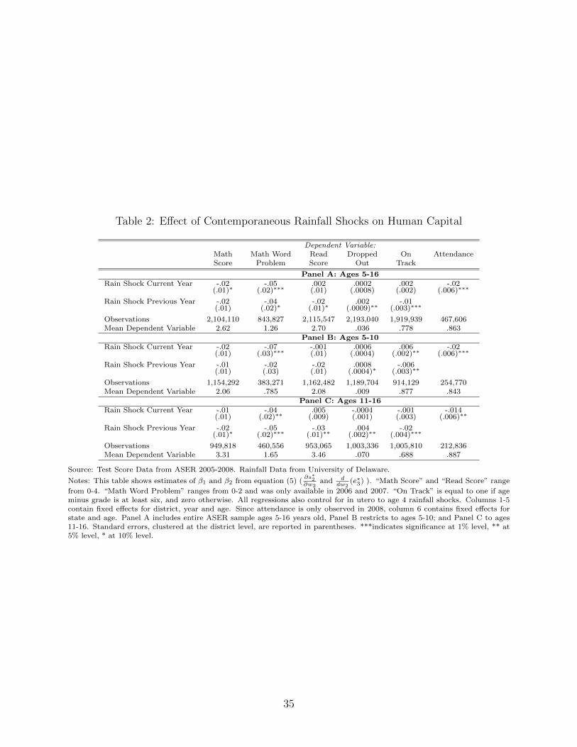
Table 2: Effect of Contemporaneous Rainfall Shocks on Human Capital

Dependent Variable:Math Math Word Read Dropped On AttendanceScore Problem Score Out Track

Panel A: Ages 5-16Rain Shock Current Year -.02 -.05 .002 .0002 .002 -.02

(.01)∗ (.02)∗∗∗ (.01) (.0008) (.002) (.006)∗∗∗

Rain Shock Previous Year -.02 -.04 -.02 .002 -.01(.01) (.02)∗ (.01)∗ (.0009)∗∗ (.003)∗∗∗

Observations 2,104,110 843,827 2,115,547 2,193,040 1,919,939 467,606Mean Dependent Variable 2.62 1.26 2.70 .036 .778 .863

Panel B: Ages 5-10Rain Shock Current Year -.02 -.07 -.001 .0006 .006 -.02

(.01) (.03)∗∗∗ (.01) (.0004) (.002)∗∗ (.006)∗∗∗

Rain Shock Previous Year -.01 -.02 -.02 .0008 -.006(.01) (.03) (.01) (.0004)∗ (.003)∗∗

Observations 1,154,292 383,271 1,162,482 1,189,704 914,129 254,770Mean Dependent Variable 2.06 .785 2.08 .009 .877 .843

Panel C: Ages 11-16Rain Shock Current Year -.01 -.04 .005 -.0004 -.001 -.014

(.01) (.02)∗∗ (.009) (.001) (.003) (.006)∗∗

Rain Shock Previous Year -.02 -.05 -.03 .004 -.02(.01)∗ (.02)∗∗∗ (.01)∗∗ (.002)∗∗ (.004)∗∗∗

Observations 949,818 460,556 953,065 1,003,336 1,005,810 212,836Mean Dependent Variable 3.31 1.65 3.46 .070 .688 .887

Source: Test Score Data from ASER 2005-2008. Rainfall Data from University of Delaware.

Notes: This table shows estimates of β1 and β2 from equation (5) (∂s∗2∂w2

and ddw2

(e∗3) ). “Math Score” and “Read Score” range

from 0-4. “Math Word Problem” ranges from 0-2 and was only available in 2006 and 2007. “On Track” is equal to one if ageminus grade is at least six, and zero otherwise. All regressions also control for in utero to age 4 rainfall shocks. Columns 1-5contain fixed effects for district, year and age. Since attendance is only observed in 2008, column 6 contains fixed effects forstate and age. Panel A includes entire ASER sample ages 5-16 years old, Panel B restricts to ages 5-10; and Panel C to ages11-16. Standard errors, clustered at the district level, are reported in parentheses. ***indicates significance at 1% level, ** at5% level, * at 10% level.

35

Table 3: Effect of Contemporaneous Rain Shocks on Schooling and Child Labor

Dependent Variable:Attends School Works

Panel A: Ages 5-16Rain Shock Current Year -.01 .005

(.003)∗∗∗ (.001)∗∗∗

Rain Shock Previous Year -.004 .001(.003) (.001)

Observations 297,470 299,271Mean Dependent Variable .795 .053

Panel B: Ages 5-10Rain Shock Current Year -.005 .002

(.004) (.0006)∗∗∗

Rain Shock Previous Year -.002 .001(.004) (.0008)

Observations 154,291 155,274Mean Dependent Variable .821 .007

Panel C: Ages 11-16Rain Shock Current Year -.02 .008

(.003)∗∗∗ (.002)∗∗∗

Rain Shock Previous Year -.008 .002(.003)∗∗ (.002)

Observations 143,179 143,997Mean Dependent Variable .766 .103

Source: Attends school and child labor from rounds 60, 61, 62, and 64 of NSS. Rainfall data from University of Delaware.

Notes: This table shows estimates of β1 and β2 from equation (5) (∂s∗2∂w2

). The coefficients represent the effect of rain shocks

on a dummy variable for whether primary activity is reported as school attendance (column 1) or working (column 2). PanelA restricts the sample to children ages 5-16, Panel B to ages 5-10; and Panel C to ages 11-16. All regressions contain districtfixed effects and control for age and sex. All columns contain controls for early life rainfall shock exposure (in utero-age 4).Standard errors, clustered at the district level, are reported in parentheses. ***indicates significance at 1% level, ** at 5% level,* at 10% level.

36

Table 4: Effect of Early Life Rainfall Shocks on Human Capital

Dependent Variable:Math Math Word Read Never OnScore Problem Score Enrolled Track

Rain Shock In Utero .01 .006 .01 -.002 .02(.004)∗∗∗ (.004) (.004)∗∗∗ (.0004)∗∗∗ (.002)∗∗∗

Rain Shock Year of Birth .01 .009 .01 -.002 .02(.004)∗∗∗ (.004)∗∗ (.004)∗∗ (.0004)∗∗∗ (.002)∗∗∗

Rain Shock at Age 1 .01 .02 .01 -.003 .02(.004)∗∗∗ (.005)∗∗∗ (.004)∗∗∗ (.0004)∗∗∗ (.002)∗∗∗

Rain Shock at Age 2 .01 .02 .01 -.003 .01(.004)∗∗ (.004)∗∗∗ (.004)∗∗∗ (.0004)∗∗∗ (.002)∗∗∗

Rain Shock at Age 3 .001 .008 .007 -.002 .003(.004) (.005)∗ (.004) (.0004)∗∗∗ (.002)

Rain Shock at Age 4 .002 -.008 .01 -.002 .005(.004) (.004)∗ (.005)∗∗∗ (.0004)∗∗∗ (.002)∗∗∗

Observations 2,350,976 843,827 2,362,940 2,405,642 2,100,717Mean Dependent Variable 2.62 1.26 2.71 .028 .781

Source: Test Score Data from ASER 2005-2009. Rainfall Data from University of Delaware.Notes: This table shows estimates of ζ from equation (6), the effect of early life rainfall shocks on current test scores and

schooling outcomes (∂s∗2∂w1

and ddw1

(e∗3)). “Math Score” and “Read Score” range from 0-4. “Math Word Problem” ranges from

0-2 and was only asked in 2006 and 2007. “On Track” is equal to one if age minus grade is at least six, and zero otherwise.All regressions contain fixed effects for household, year and age. Standard errors, clustered at the district level, are reported inparentheses. ***indicates significance at 1% level, ** at 5% level, * at 10% level.

Table 5: Effect of Rainfall Shocks on Child Weight

Weight for age z-score

Rain Shock Current Year .12(.05)∗∗

Rain Shock Previous Year .22(.06)∗∗∗

Observations 15,307Mean Dependent Variable -1.516

Source: Data on child weight from IDHS in 2004-2005. Rainfall Data from University of Delaware.Notes: This table shows estimates of the effect of rainfall shocks on weight for age z-scores for children ages 1–5 (or ∂c1

∂w1).

These are anthropometric z-scores using the 2006 WHO child growth standards. The regression contains age, year, and statefixed effects. Standard errors, clustered at the district level, are reported in parentheses. ***indicates significance at 1% level,** at 5% level, * at 10% level.

37

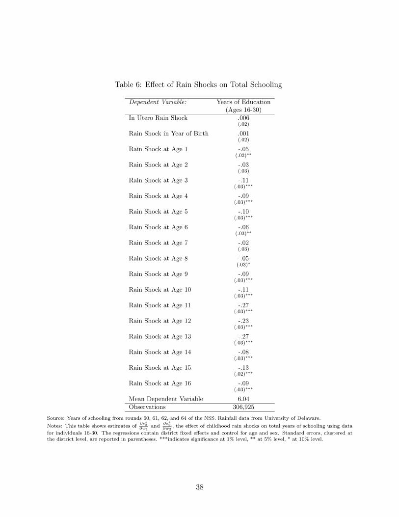
Table 6: Effect of Rain Shocks on Total Schooling

Dependent Variable: Years of Education(Ages 16-30)

In Utero Rain Shock .006(.02)

Rain Shock in Year of Birth .001(.02)

Rain Shock at Age 1 -.05(.02)∗∗

Rain Shock at Age 2 -.03(.03)

Rain Shock at Age 3 -.11(.03)∗∗∗

Rain Shock at Age 4 -.09(.03)∗∗∗

Rain Shock at Age 5 -.10(.03)∗∗∗

Rain Shock at Age 6 -.06(.03)∗∗

Rain Shock at Age 7 -.02(.03)

Rain Shock at Age 8 -.05(.03)∗

Rain Shock at Age 9 -.09(.03)∗∗∗

Rain Shock at Age 10 -.11(.03)∗∗∗

Rain Shock at Age 11 -.27(.03)∗∗∗

Rain Shock at Age 12 -.23(.03)∗∗∗

Rain Shock at Age 13 -.27(.03)∗∗∗

Rain Shock at Age 14 -.08(.03)∗∗∗

Rain Shock at Age 15 -.13(.02)∗∗∗

Rain Shock at Age 16 -.09(.03)∗∗∗

Mean Dependent Variable 6.04Observations 306,925

Source: Years of schooling from rounds 60, 61, 62, and 64 of the NSS. Rainfall data from University of Delaware.

Notes: This table shows estimates of∂s∗2∂w1

and∂s∗2∂w2

, the effect of childhood rain shocks on total years of schooling using data

for individuals 16-30. The regressions contain district fixed effects and control for age and sex. Standard errors, clustered atthe district level, are reported in parentheses. ***indicates significance at 1% level, ** at 5% level, * at 10% level.

38

-0.004

-0.002

0

0.002

0.004

0.006

0.008

0.01

0.012

0.014

0.016

5 6 7 8 9 10 11 12 13 14 15

Coef

ficie

nt

Age at Rainfall Shock

Coefficient of Rain Shock Last Year at Each Age on Drop Out

Dropout

95% CI

Figure 1: Effect of Rainfall Shocks Last Year on Current Test Scores

-­‐0.4  

-­‐0.35  

-­‐0.3  

-­‐0.25  

-­‐0.2  

-­‐0.15  

-­‐0.1  

-­‐0.05  

0  

0.05  

0.1  

-­‐2   0   2   4   6   8   10   12   14   16   18  

Coeffi

cien

t  

Age  at  Rainfall  Shock  

Coefficient  of  Rain  Shock  at  Each  Age  on  Total  Years  of  Schooling  

Schooling  

95%  CI  

Figure 2: Effect of Rainfall Shocks on Total Years of Schooling

39

A Appendix Tables

40

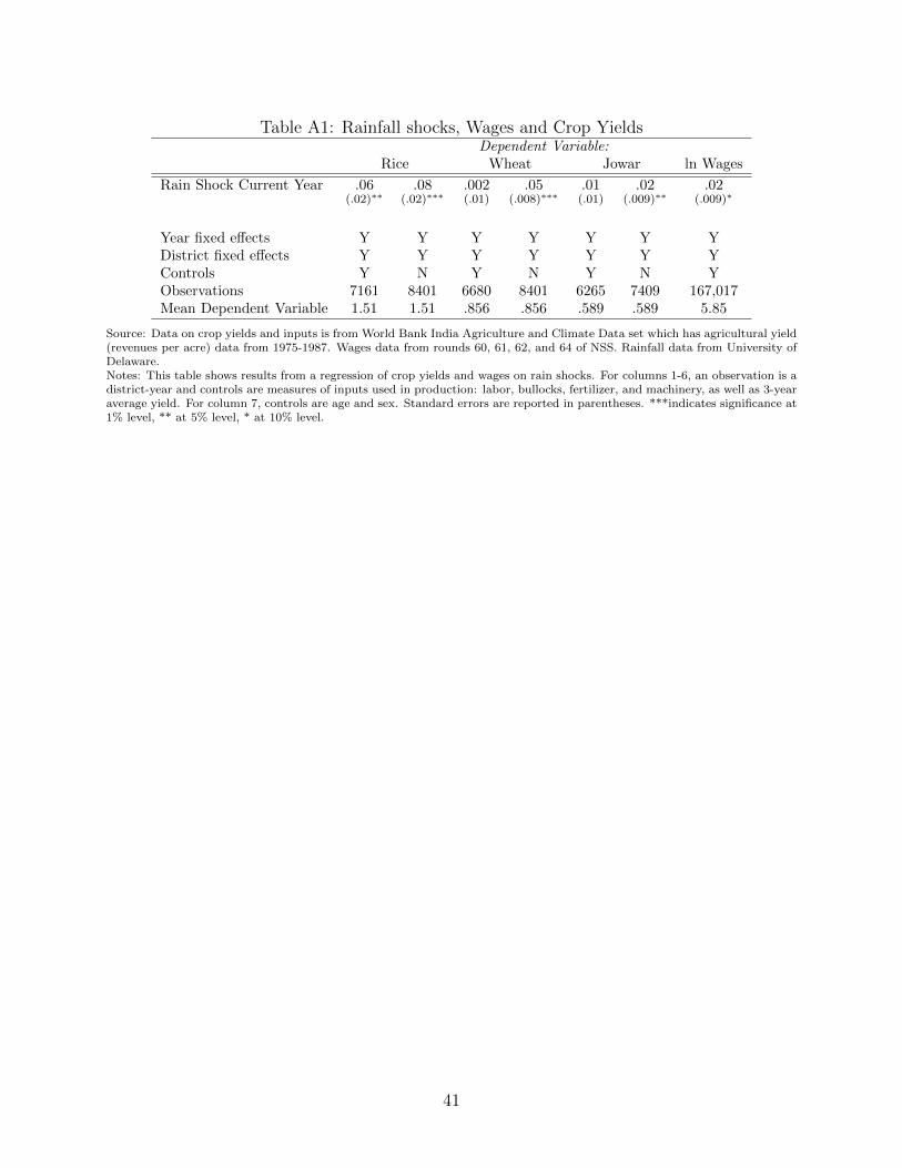
Table A1: Rainfall shocks, Wages and Crop YieldsDependent Variable:

Rice Wheat Jowar ln Wages

Rain Shock Current Year .06 .08 .002 .05 .01 .02 .02(.02)∗∗ (.02)∗∗∗ (.01) (.008)∗∗∗ (.01) (.009)∗∗ (.009)∗

Year fixed effects Y Y Y Y Y Y YDistrict fixed effects Y Y Y Y Y Y YControls Y N Y N Y N YObservations 7161 8401 6680 8401 6265 7409 167,017Mean Dependent Variable 1.51 1.51 .856 .856 .589 .589 5.85

Source: Data on crop yields and inputs is from World Bank India Agriculture and Climate Data set which has agricultural yield(revenues per acre) data from 1975-1987. Wages data from rounds 60, 61, 62, and 64 of NSS. Rainfall data from University ofDelaware.Notes: This table shows results from a regression of crop yields and wages on rain shocks. For columns 1-6, an observation is adistrict-year and controls are measures of inputs used in production: labor, bullocks, fertilizer, and machinery, as well as 3-yearaverage yield. For column 7, controls are age and sex. Standard errors are reported in parentheses. ***indicates significance at1% level, ** at 5% level, * at 10% level.

41

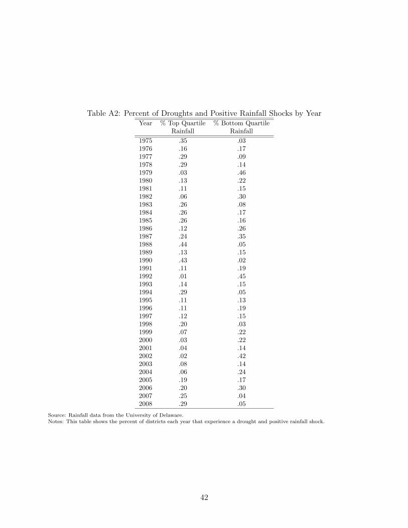
Table A2: Percent of Droughts and Positive Rainfall Shocks by YearYear % Top Quartile % Bottom Quartile

Rainfall Rainfall

1975 .35 .031976 .16 .171977 .29 .091978 .29 .141979 .03 .461980 .13 .221981 .11 .151982 .06 .301983 .26 .081984 .26 .171985 .26 .161986 .12 .261987 .24 .351988 .44 .051989 .13 .151990 .43 .021991 .11 .191992 .01 .451993 .14 .151994 .29 .051995 .11 .131996 .11 .191997 .12 .151998 .20 .031999 .07 .222000 .03 .222001 .04 .142002 .02 .422003 .08 .142004 .06 .242005 .19 .172006 .20 .302007 .25 .042008 .29 .05

Source: Rainfall data from the University of Delaware.Notes: This table shows the percent of districts each year that experience a drought and positive rainfall shock.

42

Table A3: Effect of Contemporaneous Rainfall Shocks on Human Capital (Ordered Logit)

Dependent Variable:Math Math ReadScore Word Problem Score

Rain Shock Current Year -.03 -.15 -.002(.02) (.07)∗∗ (.02)

Rain Shock Previous Year -.03 -.15 -.04(.02) (.08)∗∗ (.02)∗

Observations 2,109,162 843,827 2,120,708

Source: Test Score Data from ASER 2005-2009. Rainfall Data from University of Delaware.Notes: This table shows ordered logit estimates of the effect of rainfall shocks on current test scores using the ASER data for allchildren ages 5-16 (or β1 and β2 from equation (5)). “Math Score” and “Read Score” range from 0-4. “Math Word Problem”ranges from 0-2 and is only available in 2006 and 2007. All regressions contain fixed effects for district, year and age. Allcolumns contain controls for early life rainfall shock exposure (in utero-age 4). Standard errors, clustered at the district level,are reported in parentheses. ***indicates significance at 1% level, ** at 5% level, * at 10% level.

43

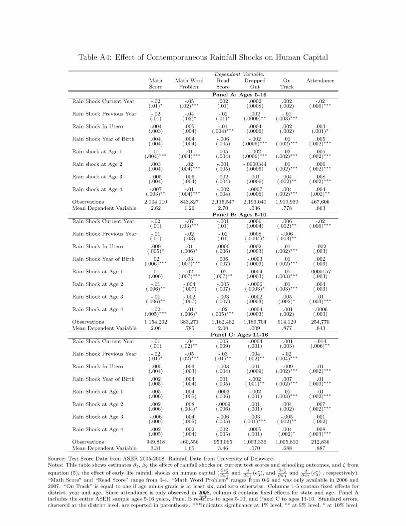
Table A4: Effect of Contemporaneous Rainfall Shocks on Human Capital

Dependent Variable:Math Math Word Read Dropped On AttendanceScore Problem Score Out Track

Panel A: Ages 5-16Rain Shock Current Year -.02 -.05 .002 .0002 .002 -.02

(.01)∗ (.02)∗∗∗ (.01) (.0008) (.002) (.006)∗∗∗

Rain Shock Previous Year -.02 -.04 -.02 .002 -.01(.01) (.02)∗ (.01)∗ (.0009)∗∗ (.003)∗∗∗

Rain Shock In Utero -.004 .005 -.01 .0004 .002 .003(.003) (.004) (.004)∗∗∗ (.0006) (.002) (.001)∗

Rain Shock Year of Birth .004 .004 -.006 -.002 .01 .005(.004) (.004) (.005) (.0006)∗∗∗ (.002)∗∗∗ (.002)∗∗∗

Rain shock at Age 1 .01 .01 .005 -.002 .02 .005(.004)∗∗∗ (.004)∗∗∗ (.004) (.0006)∗∗∗ (.002)∗∗∗ (.002)∗∗∗

Rain shock at Age 2 .003 .02 -.001 -.0000344 .01 .006(.004) (.004)∗∗∗ (.005) (.0006) (.002)∗∗∗ (.002)∗∗∗

Rain shock at Age 3 -.005 .006 .002 .001 .004 .008(.004) (.004) (.004) (.0006) (.002)∗∗ (.002)∗∗∗

Rain shock at Age 4 -.007 -.01 -.002 -.0007 .004 .004(.003)∗∗ (.004)∗∗∗ (.004) (.0006) (.002)∗∗∗ (.002)∗∗

Observations 2,104,110 843,827 2,115,547 2,193,040 1,919,939 467,606Mean Dependent Variable 2.62 1.26 2.70 .036 .778 .863

Panel B: Ages 5-10Rain Shock Current Year -.02 -.07 -.001 .0006 .006 -.02

(.01) (.03)∗∗∗ (.01) (.0004) (.002)∗∗ (.006)∗∗∗

Rain Shock Previous Year -.01 -.02 -.02 .0008 -.006(.01) (.03) (.01) (.0004)∗ (.003)∗∗

Rain Shock In Utero .009 .01 .0006 .0002 .01 -.002(.005)∗ (.006)∗ (.006) (.0003) (.002)∗∗∗ (.003)

Rain Shock Year of Birth .02 .03 .006 -.0003 .01 .002(.006)∗∗∗ (.007)∗∗∗ (.007) (.0003) (.002)∗∗∗ (.003)

Rain Shock at Age 1 .01 .02 .02 -.0004 .01 .0000157(.006) (.007)∗∗∗ (.007)∗∗ (.0003) (.003)∗∗∗ (.003)

Rain Shock at Age 2 -.01 -.004 -.005 -.0006 .01 .004(.006)∗∗ (.007) (.007) (.0003)∗ (.003)∗∗∗ (.003)

Rain Shock at Age 3 -.01 -.002 -.003 -.0002 .005 .01(.006)∗∗ (.007) (.007) (.0003) (.002)∗ (.003)∗∗∗

Rain Shock at Age 4 -.02 -.01 -.02 -.0004 -.001 -.0006(.005)∗∗∗ (.006)∗ (.005)∗∗∗ (.0003) (.002) (.003)

Observations 1,154,292 383,271 1,162,482 1,189,704 914,129 254,770Mean Dependent Variable 2.06 .785 2.08 .009 .877 .843

Panel C: Ages 11-16Rain Shock Current Year -.01 -.04 .005 -.0004 -.001 -.014

(.01) (.02)∗∗ (.009) (.001) (.003) (.006)∗∗

Rain Shock Previous Year -.02 -.05 -.03 .004 -.02(.01)∗ (.02)∗∗∗ (.01)∗∗ (.002)∗∗ (.004)∗∗∗

Rain Shock In Utero -.005 .003 -.003 .001 -.009 .01(.004) (.003) (.004) (.0009) (.002)∗∗∗ (.002)∗∗∗

Rain Shock Year of Birth .002 .004 .001 -.002 .007 .01(.005) (.004) (.005) (.001)∗∗ (.002)∗∗∗ (.003)∗∗∗

Rain Shock at Age 1 .005 .004 .0003 -.002 .01 .01(.006) (.005) (.006) (.001) (.003)∗∗∗ (.002)∗∗∗

Rain Shock at Age 2 .002 .008 -.0009 .001 .004 .007(.006) (.004)∗ (.006) (.001) (.002) (.002)∗∗∗

Rain Shock at Age 3 -.006 .004 -.006 .003 -.005 .001(.006) (.005) (.005) (.001)∗∗∗ (.002)∗∗ (.002)

Rain Shock at Age 4 .002 .002 .002 .0005 .004 .008(.005) (.004) (.005) (.001) (.002)∗ (.003)∗∗∗

Observations 949,818 460,556 953,065 1,003,336 1,005,810 212,836Mean Dependent Variable 3.31 1.65 3.46 .070 .688 .887

Source: Test Score Data from ASER 2005-2008. Rainfall Data from University of Delaware.Notes: This table shows estimates β1, β2 the effect of rainfall shocks on current test scores and schooling outcomes, and ζ from

equation (5), the effect of early life rainfall shocks on human capital (∂s∗2dw2

and ddw2

(e∗3), and∂s∗2∂w1

and d∂w1

(e∗3) , respectively).

“Math Score” and “Read Score” range from 0-4. “Math Word Problem” ranges from 0-2 and was only available in 2006 and2007. “On Track” is equal to one if age minus grade is at least six, and zero otherwise. Columns 1-5 contain fixed effects fordistrict, year and age. Since attendance is only observed in 2008, column 6 contains fixed effects for state and age. Panel Aincludes the entire ASER sample ages 5-16 years, Panel B restricts to ages 5-10; and Panel C to ages 11-16. Standard errors,clustered at the district level, are reported in parentheses. ***indicates significance at 1% level, ** at 5% level, * at 10% level.

44

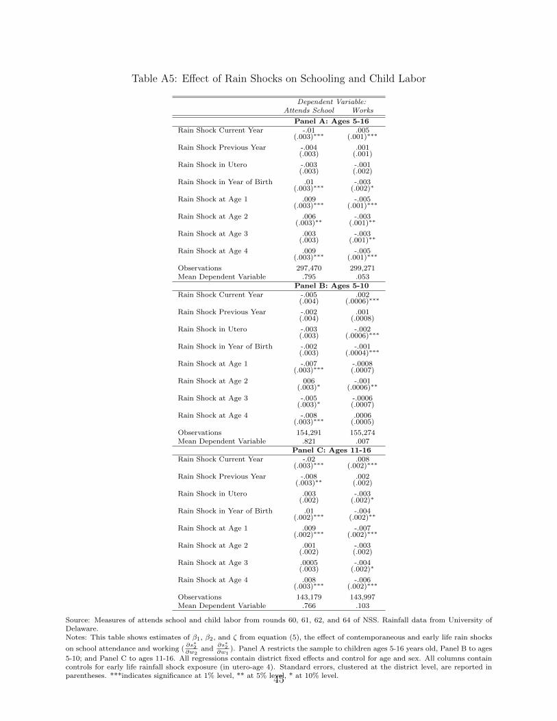
Table A5: Effect of Rain Shocks on Schooling and Child Labor

Dependent Variable:Attends School Works

Panel A: Ages 5-16Rain Shock Current Year -.01 .005

(.003)∗∗∗ (.001)∗∗∗

Rain Shock Previous Year -.004 .001(.003) (.001)

Rain Shock in Utero -.003 -.001(.003) (.002)

Rain Shock in Year of Birth .01 -.003(.003)∗∗∗ (.002)∗

Rain Shock at Age 1 .009 -.005(.003)∗∗∗ (.001)∗∗∗

Rain Shock at Age 2 .006 -.003(.003)∗∗ (.001)∗∗

Rain Shock at Age 3 .003 -.003(.003) (.001)∗∗

Rain Shock at Age 4 .009 -.005(.003)∗∗∗ (.001)∗∗∗

Observations 297,470 299,271Mean Dependent Variable .795 .053

Panel B: Ages 5-10Rain Shock Current Year -.005 .002

(.004) (.0006)∗∗∗

Rain Shock Previous Year -.002 .001(.004) (.0008)

Rain Shock in Utero -.003 -.002(.003) (.0006)∗∗∗

Rain Shock in Year of Birth -.002 -.001(.003) (.0004)∗∗∗

Rain Shock at Age 1 -.007 -.0008(.003)∗∗∗ (.0007)

Rain Shock at Age 2 006 -.001(.003)∗ (.0006)∗∗

Rain Shock at Age 3 -.005 -.0006(.003)∗ (.0007)

Rain Shock at Age 4 -.008 .0006(.003)∗∗∗ (.0005)

Observations 154,291 155,274Mean Dependent Variable .821 .007

Panel C: Ages 11-16Rain Shock Current Year -.02 .008

(.003)∗∗∗ (.002)∗∗∗

Rain Shock Previous Year -.008 .002(.003)∗∗ (.002)

Rain Shock in Utero .003 -.003(.002) (.002)∗

Rain Shock in Year of Birth .01 -.004(.002)∗∗∗ (.002)∗∗

Rain Shock at Age 1 .009 -.007(.002)∗∗∗ (.002)∗∗∗

Rain Shock at Age 2 .001 -.003(.002) (.002)

Rain Shock at Age 3 .0005 -.004(.003) (.002)∗

Rain Shock at Age 4 .008 -.006(.003)∗∗∗ (.002)∗∗∗

Observations 143,179 143,997Mean Dependent Variable .766 .103

Source: Measures of attends school and child labor from rounds 60, 61, 62, and 64 of NSS. Rainfall data from University ofDelaware.Notes: This table shows estimates of β1, β2, and ζ from equation (5), the effect of contemporaneous and early life rain shocks

on school attendance and working (∂s∗2∂w2

and∂s∗2∂w1

). Panel A restricts the sample to children ages 5-16 years old, Panel B to ages

5-10; and Panel C to ages 11-16. All regressions contain district fixed effects and control for age and sex. All columns containcontrols for early life rainfall shock exposure (in utero-age 4). Standard errors, clustered at the district level, are reported inparentheses. ***indicates significance at 1% level, ** at 5% level, * at 10% level.45

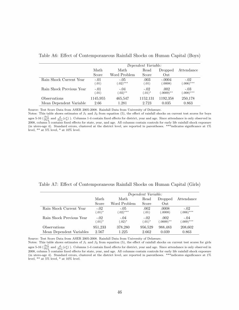
Table A6: Effect of Contemporaneous Rainfall Shocks on Human Capital (Boys)

Dependent Variable:Math Math Read Dropped AttendanceScore Word Problem Score Out

Rain Shock Current Year -.01 -.05 .003 -.0004 -.02(.01) (.02)∗∗∗ (.01) (.0008) (.006)∗∗∗

Rain Shock Previous Year -.01 -.04 -.02 .002 -.03(.01) (.02)∗∗ (.01)∗ (.0009)∗∗ (.008)∗∗∗

Observations 1145,955 465,547 1152,131 1192,358 250,178Mean Dependent Variable 2.66 1.281 2.723 0.035 0.863

Source: Test Score Data from ASER 2005-2008. Rainfall Data from University of Delaware.Notes: This table shows estimates of β1 and β2 from equation (5), the effect of rainfall shocks on current test scores for boys

ages 5-16 (∂s∗2∂w2

and ddw2

(e∗3) ). Columns 1-4 contain fixed effects for district, year and age. Since attendance is only observed in

2008, column 5 contains fixed effects for state, year, and age. All columns contain controls for early life rainfall shock exposure(in utero-age 4). Standard errors, clustered at the district level, are reported in parentheses. ***indicates significance at 1%level, ** at 5% level, * at 10% level.

Table A7: Effect of Contemporaneous Rainfall Shocks on Human Capital (Girls)

Dependent Variable:Math Math Read Dropped AttendanceScore Word Problem Score Out

Rain Shock Current Year -.02 -.05 .002 .0008 -.02(.01)∗ (.02)∗∗∗ (.01) (.0008) (.006)∗∗∗

Rain Shock Previous Year -.02 -.04 -.02 .002 -.04(.01)∗ (.02)∗ (.01)∗ (.0009)∗∗ (.009)∗∗∗

Observations 951,233 378,280 956,529 988,483 208,602Mean Dependent Variables 2.567 1.225 2.662 0.039 0.863

Source: Test Score Data from ASER 2005-2008. Rainfall Data from University of Delaware.Notes: This table shows estimates of β1 and β2 from equation (5), the effect of rainfall shocks on current test scores for girls

ages 5-16 (∂s∗2∂w2

and ddw2

(e∗3) ). Columns 1-4 contain fixed effects for district, year and age. Since attendance is only observed in

2008, column 5 contains fixed effects for state, year, and age. All columns contain controls for early life rainfall shock exposure(in utero-age 4). Standard errors, clustered at the district level, are reported in parentheses. ***indicates significance at 1%level, ** at 5% level, * at 10% level.

46

Table A8: Effect of Early Life Rainfall Shocks on Human Capital (Boys)

Dependent Variable:Math Math Read Never OnScore Word Problem Score Enrolled Track

Rain Shock In Utero .008 .003 .01 -.001 .02(.004)∗ (.006) (.005)∗∗ (.0004)∗∗∗ (.002)∗∗∗

Rain Shock Year of Birth .01 .01 .008 -.002 .02(.004)∗∗ (.006)∗ (.004)∗ (.0004)∗∗∗ (.002)∗∗∗

Rain Shock at Age 1 .01 .02 .01 -.002 .01(.005)∗∗ (.006)∗∗∗ (.005)∗∗ (.0005)∗∗∗ (.002)∗∗∗

Rain Shock at Age 2 .01 .02 .01 -.003 .01(.004)∗∗∗ (.006)∗∗∗ (.004)∗∗∗ (.0004)∗∗∗ (.002)∗∗∗

Rain Shock at Age 3 .006 .01 .01 -.002 -.0002(.005) (.006)∗∗ (.005)∗∗ (.0004)∗∗∗ (.002)

Rain Shock at Age 4 .003 -.008 .01 -.002 .002(.005) (.006) (.005)∗∗ (.0004)∗∗∗ (.002)

Observations 1,271,233 465,547 1,277,571 1,297,538 959,304Mean Dependent Variable 2.66 1.281 2.723 0.026 0.811

Source: Test Score Data from ASER 2005-2009. Rainfall Data from University of Delaware.Notes: This table shows estimates of ζ from equation (6), the effect of early life rainfall shocks on current test scores and

schooling outcomes restricted to boys only (∂s∗2∂w1

and ddw1

(e∗3) ). “Math Score” and “Read Score” range from 0-4. “Math Word

Problem” ranges from 0-2, and was only asked in 2006 and 2007. “On Track” is equal to one if age minus grade is at least six,and zero otherwise. All regressions contain fixed effects for household, year and age. Standard errors, clustered at the districtlevel, are reported in parentheses. ***indicates significance at 1% level, ** at 5% level, * at 10% level.

Table A9: Effect of Early Life Rainfall Shocks on Human Capital (Girls)

Dependent Variable:maths Math Read Never Onscore Word Problem Score Enrolled Track

Rain Shock in Utero .02 .009 .02 -.002 .03(.005)∗∗∗ (.006) (.005)∗∗∗ (.0006)∗∗∗ (.003)∗∗∗

Rain Shock Year of Birth .01 .005 .01 -.002 .02(.005)∗∗ (.007) (.006)∗∗ (.0006)∗∗∗ (.003)∗∗∗

Rain Shock at Age 1 .01 .01 .02 -.003 .02(.005)∗∗∗ (.007) (.005)∗∗∗ (.0005)∗∗∗ (.003)∗∗∗

Rain Shock at Age 2 .007 .01 .01 -.003 .01(.005) (.007)∗∗ (.005)∗∗ (.0006)∗∗∗ (.003)∗∗∗

Rain Shock at Age 3 -.005 -.002 .002 -.001 -.0002(.005) (.007) (.005) (.0006)∗ (.002)

Rain Shock at Age 4 -.003 -.01 .009 -.002 .0000306(.005) (.007)∗ (.005)∗ (.0005)∗∗∗ (.002)

Observations 1,057,467 378,280 1,062,888 1,079,939 808,469Mean Dependent Variable 2.567 1.225 2.662 0.035 0.811

Source: Test Score Data from ASER 2005-2009. Rainfall Data from University of Delaware.Notes: This table shows estimates of ζ from equation (6), the effect of early life rainfall shocks on current test scores and

schooling outcomes restricted to girls only (∂s∗2∂w1

and ddw1

(e∗3) ). “Math Score” and “Read Score” range from 0-4. “Math Word

Problem” ranges from 0-2, and was only asked in 2006 and 2007. “On Track” is equal to one if age minus grade is at least six,and zero otherwise. All regressions contain fixed effects for household, year and age. Standard errors, clustered at the districtlevel, are reported in parentheses. ***indicates significance at 1% level, ** at 5% level, * at 10% level.

47

Table A10: Effect of Rain Shocks on Days Sick and Health Expenditures

Days Healthsick expenditures (ln Rs)

Rain Shock Current Year -.52 -.22(.22)∗∗ (.07)∗∗∗

Rain Shock Previous Year -.38 .005(.22)∗ (.1)

Observations 6293 6293Mean Dependent Variable 6.07 4.28

Source: IHDS 2004–2005 data for children ages 5-16. Rainfall data from the University of Delaware.Notes: This table shows estimates of the effect of rainfall shocks on number of days sick in last month due to diarrhea, fever,and/or cough and health expenditures (hospital, doctor, medicine, tests, and transport) for children ages 5-16. Each cell is aseparate OLS regression. All regressions contain age, gender and state fixed effects. Standard errors, clustered at the districtlevel, are reported in parentheses. ***indicates significance at 1% level, ** at 5% level, * at 10% level.

Table A11: Effect of Rain Shocks on Test Scores in High Malaria States

Dependent Variable:Math ReadingScore Score

Rain Shock Current Year -.08 -.03(.03)∗∗ (.03)

Malaria state -.14 -.1(.12) (.12)

Rain shock*Malaria state .07 .03(.07) (.06)

Rain Shock Previous Year .04 .02(.03) (.03)

Observations 1,892,741 2,115,547

Source: Test Score Data from ASER 2005-2009. Rainfall Data from University of Delaware.Notes: This table shows estimates β1, the effect of rainfall shocks on current test scores and schooling outcomes interacted witha dummy for the five high malaria states (Orissa, Chhattisgarh, West Bengal, Jharkhand, and Karnataka). All specificationsinclude state-region fixed effects and are clustered at the state level. All columns contain controls for early life rainfall shockexposure (in utero-age 4). Standard errors, clustered at the district level, are reported in parentheses. ***indicates significanceat 1% level, ** at 5% level, * at 10% level.

Table A12: Are Teacher Absences or School Lunches Driving the Results?

Dependent Variable: Teacher Absence Rate Midday Meal Provision

Rain Shock Current Year -.03 .04(.01)∗∗ (.02)∗∗

Rain Shock Previous Year .002 .06(.01) (.02)∗∗∗

Observations 20,297 24,203Mean Dependent Variable 0.18 0.81

Source: Teacher absence rates and midday meal provision data from the 2005 and 2007 ASER School Survey.Notes: This table shows the coefficients of rainfall shocks on teacher absence rates and midday meal provision in a linearregression. All regressions contain village and year fixed effects. Standard errors, clustered at the district level, are reported inparentheses. ***indicates significance at 1% level, ** at 5% level, * at 10% level.

48

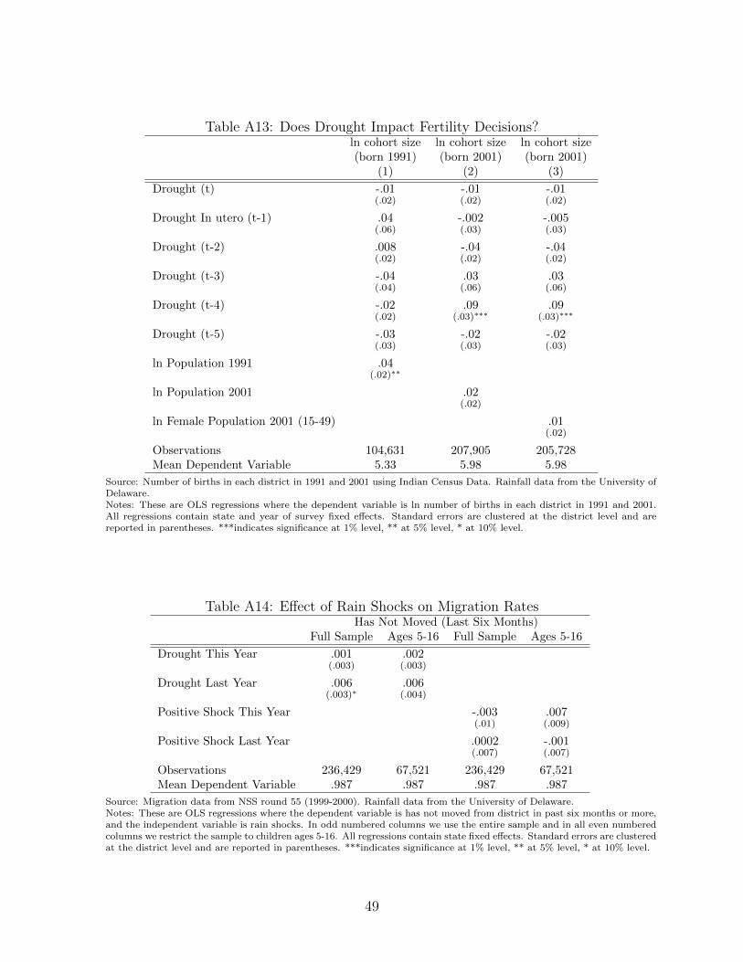
Table A13: Does Drought Impact Fertility Decisions?ln cohort size ln cohort size ln cohort size(born 1991) (born 2001) (born 2001)

(1) (2) (3)

Drought (t) -.01 -.01 -.01(.02) (.02) (.02)

Drought In utero (t-1) .04 -.002 -.005(.06) (.03) (.03)

Drought (t-2) .008 -.04 -.04(.02) (.02) (.02)

Drought (t-3) -.04 .03 .03(.04) (.06) (.06)

Drought (t-4) -.02 .09 .09(.02) (.03)∗∗∗ (.03)∗∗∗

Drought (t-5) -.03 -.02 -.02(.03) (.03) (.03)

ln Population 1991 .04(.02)∗∗

ln Population 2001 .02(.02)

ln Female Population 2001 (15-49) .01(.02)

Observations 104,631 207,905 205,728Mean Dependent Variable 5.33 5.98 5.98

Source: Number of births in each district in 1991 and 2001 using Indian Census Data. Rainfall data from the University ofDelaware.Notes: These are OLS regressions where the dependent variable is ln number of births in each district in 1991 and 2001.All regressions contain state and year of survey fixed effects. Standard errors are clustered at the district level and arereported in parentheses. ***indicates significance at 1% level, ** at 5% level, * at 10% level.

Table A14: Effect of Rain Shocks on Migration RatesHas Not Moved (Last Six Months)

Full Sample Ages 5-16 Full Sample Ages 5-16

Drought This Year .001 .002(.003) (.003)

Drought Last Year .006 .006(.003)∗ (.004)

Positive Shock This Year -.003 .007(.01) (.009)

Positive Shock Last Year .0002 -.001(.007) (.007)

Observations 236,429 67,521 236,429 67,521Mean Dependent Variable .987 .987 .987 .987

Source: Migration data from NSS round 55 (1999-2000). Rainfall data from the University of Delaware.Notes: These are OLS regressions where the dependent variable is has not moved from district in past six months or more,and the independent variable is rain shocks. In odd numbered columns we use the entire sample and in all even numberedcolumns we restrict the sample to children ages 5-16. All regressions contain state fixed effects. Standard errors are clusteredat the district level and are reported in parentheses. ***indicates significance at 1% level, ** at 5% level, * at 10% level.

49

Mathematical Appendix

Parents maximize total household utility:

maxc2,s2

{u1(c1) + βu2(c2) + β2V (e3)

}subject to the constraints that

c2 ≤ w2(h+ (1− s2)e2)

c1 ≤ w1h

s2 ∈ [0, 1]

e3 = f3 (e2, c2, s2) = f3 (e2, w2(h+ (1− s2)e2), s2)

and we have assumed that

V (e3) = e3

Since no decisions are made in the first period, we can rewrite the maximization problem

as

maxs2∈[0,1],c2

{u2 (c2) + βf3 (e2, c2, s2)} s.t. c2 ≤ w2 (h+ (1− s2) e2)

The Lagrangian for this problem is:

L = u2(c2) + βf3 (e2, s2, c2) + λ [w2 (h+ (1− s2) e2)− c2]

Given the assumptions laid out in Section 2, the first order conditions will be necessary

and sufficient to characterize a unique optimum:

50

∂L∂λ

= w2 (h+ (1− s∗2 (w2, e2) e2))− c∗2 (w2, e2) = 0

∂L∂c2

= u′ (c∗2 (w2, e2)) + β∂f3

∂c2

(e2, c∗2 (w2, e2) , s∗2 (w2, e2))− λ∗ (w2, e2) = 0

∂L∂s2

= β∂f3

∂s2

(e2, c∗2 (w2, e2) , s∗2 (w2, e2))− λ∗ (w2, e2) · w2e2 = 0

Rearranging yields the single first-order condition outlined in the text of Section 2:

w2e2∂u2

∂c2

= β

(∂f3

∂s2

− w2e2∂f3

∂c2

)We define the function

Θ(w2, e2, c∗2, s∗2) =

(∂f3

∂s2

− w2e2∂f3

∂c2

)so we can rewrite the first order condition as

w2e2∂u2

∂c2

= βΘ

Effect of School-Aged Wages on Schooling and Human Capital

Beginning from the first order condition,

F.O.C.: w2e2∂u2

∂c2

= β

(∂f3

∂s2

− w2e2∂f3

∂c2

)We can take the total derivative with respect to w2 (noting that e2 = f2 (w1h) and

e3 = f3 (w1h,w2(h+ (1− s2)e2), s2):

[∂2u2

∂c22

w2e2

((h+ (1− s∗2) e2)− w2e2

∂s∗2∂w2

)+ e2

∂u2

∂c2

]=

51

β

[∂2f3

∂s2∂c2

((h+ (1− s∗2) e2)− w2e2

∂s∗2∂w2

)+∂2f3

∂s22

∂s∗2∂w2

]

−β[(

∂2f3

∂c22

((h+ (1− s∗2) e2)− w2e2

∂s∗2∂w2

)+

∂2f3

∂c2∂s2

∂s∗2∂w2

)e2w2 + e2

∂f3

∂c2

]and solve for

∂s∗2∂w2

∂s∗2∂w2

=

∂2u2∂c22

w2e2 (h+ (1− s∗2) e2) + e2∂u2∂c2− β

[∂2f3∂s2∂c2

(h+ (1− s∗2) e2)− ∂2f3∂c22

(h+ (1− s∗2) e2) e2w2 − e2∂f3∂c2

]w2

2e22∂2u2∂c22

+ β[∂2f3∂s22

+ w22e

22∂2f3∂c22− 2e2w2

∂2f3∂c2∂s2

]Since, by assumption

w22e

22

∂2u2

∂c22

+ β

[∂2f3

∂s22

+ w22e

22

∂2f3

∂c22

− 2e2w2∂2f3

∂c2∂s2

]< 0

we can write that

∂s∗2∂w2

∝ −∂2u2

∂c22

w2e2 (h+ (1− s∗2) e2)− e2∂u2

∂c2

+β

[∂2f3

∂s2∂c2

(h+ (1− s∗2) e2)− ∂2f3

∂c22

(h+ (1− s∗2) e2) e2w2 − e2∂f3

∂c2

]Rearranging slightly,

∂s∗2∂w2

∝ −e2

(∂u2

∂c2

+ β∂f3

∂c2

)−(h+ (1− s∗2) e2)w2e2

∂2u2

∂c22

+(h+ (1− s∗2) e2) β

[∂2f3

∂s2∂c2

− ∂2f3

∂c22

e2w2

]

And since

Θ =∂f3

∂s2

− w2e2∂f3

∂c2

52

∂Θ

∂c2

=∂2f3

∂s2∂c2

− e2w2∂2f3

∂c22

And substituting this into the above equation yields

∂s∗2∂w2

∝ −e2

(∂u2

∂c2

+ β∂f3

∂c2

)− (h+ (1− s∗2) e2)w2e2

∂2u2

∂c22

+ (h+ (1− s∗2) e2) β∂Θ

∂c2

In addition, since we know that

e∗3 = f3 (e2, c∗2, s∗2)

we can write the effect of school-aged wages on later-life human capital:

d

dw2

(f3 (e2, c∗2, s∗2)) =

∂f3

∂c2

∂c∗2∂w2

+∂f3

∂s2

∂s∗2∂w2

=∂f3

∂c2

(h+ (1− s∗2)e2 − w2e2

∂s∗2∂w2

)+∂f3

∂s2

∂s∗2∂w2

= (h+ (1− s2)e2)∂f3

∂c2

+ Θ∂s∗2∂w2

Effect of Early Life Wages on Schooling and Human Capital

Beginning from the first order condition,

F.O.C.:∂u2

∂c2

w2e2 = β

(∂f3

∂s2

− w2e2∂f3

∂c2

)Noting as in the text, that

d

dw1

(e2) =∂f2

∂c1

∂c1

∂w1

= h∂f2

∂c1

> 0

and in order to understand the effect of early life wages on schooling and later-life human

53

capital, it is sufficient to study the effect of period 2 human capital on these variables:

∂s∗2∂w1

= h∂f2

∂c1

∂s∗2∂e2

∝ ∂s∗2∂e2

We can take the total derivative of the first order condition with respect to e2 (noting

that e2 = f2 (w1h) and e3 = f3 (w1h,w2(h+ (1− s2)e2), s2):

w2e2

(w2 (1− s∗2)− w2e2

∂s∗2∂e2

)∂2u2

∂c22

+ w2∂u2

∂c2

=

β

[∂2f3

∂s2∂e2

+∂2f3

∂s2∂c2

(w2 (1− s∗2)− w2e2

∂s∗2∂e2

)+∂2f3

∂s22

∂s∗2∂e2

]

−β[w2e2

(∂2f3

∂c2∂e2

+∂2f3

∂c22

(w2 (1− s∗2)− w2e2

∂s∗2∂e2

)+

∂2f3

∂c2∂s2

∂s∗2∂e2

)+ w2

∂f3

∂c2

]Rearranging, we have

∂s∗2∂e2

=−w2

2e2 (1− s∗2) ∂2u2∂c22− w2

∂u2∂c2

+ β[

∂2f3∂s2∂e2

+ w2 (1− s∗2)(

∂2f3∂s2∂c2

− w2e2∂2f3∂c22

)− w2e2

∂2f3∂c2∂e2

− w2∂f3∂c2

]−w2

2e22∂2u2∂c22− β

[∂2f3∂s22− 2w2e2

∂2f3∂s2∂c2

+ w22e

22∂2f3∂c22

]and since, by assumption,

−w22e

22

∂2u2

∂c22

− β[∂2f3

∂s22

− 2w2e2∂2f3

∂s2∂c2

+ w22e

22

∂2f3

∂c22

]> 0

∂s∗2∂e2

∝ −w22e2 (1− s∗2)

∂2u2

∂c22

− w2∂u2

∂c2

+

β

[∂2f3

∂s2∂e2

+ w2 (1− s∗2)

(∂2f3

∂s2∂c2

− w2e2∂2f3

∂c22

)− w2e2

∂2f3

∂c2∂e2

− w2∂f3

∂c2

]and since

Θ =∂f3

∂s2

− w2e2∂f3

∂c2

54

we can rewrite this expression as

∂s∗2∂e2

∝ −w22e2 (1− s∗2)

∂2u2

∂c22

− w2∂u2

∂c2

+ β

[∂Θ

∂e2

+ w2 (1− s∗2)∂Θ

∂c2

]In addition, since we know that

e∗3 = f3 (e2, c∗2, s∗2)

we can write the effect of school-aged human capital on later-life human capital:

d

de2

(e∗3) =∂f3

∂e2

+∂f3

∂c2

∂c∗2∂e2

+∂f3

∂s2

∂s∗2∂e2

=∂f3

∂e2

+∂f3

∂c2

(w2 (1− s∗2)− w2e2

∂s∗2∂e2

)+∂f3

∂s2

∂s∗2∂e2

=∂f3

∂e2

+∂f3

∂c2

w2 (1− s∗2) + Θ∂s∗2∂e2

Discussion Section 4.4

From Equation 1,

∂s∗2∂w2

∝ −e2

(∂u2

∂c2

+ β∂f3

∂c2

)− (h+ (1− s∗2) e2)w2e2

∂2u2

∂c22

+ (h+ (1− s∗2) e2) β∂Θ

∂c2

Combined with our empirical finding that∂s∗2∂w2

< 0 implies that

− (h+ (1− s∗2) e2)w2e2∂2u2

∂c22

+ (h+ (1− s∗2) e2) β∂Θ

∂c2

< e2

(∂u2

∂c2

+ β∂f3

∂c2

)Rearranging,

55

w22e2 (1− s∗2)

∂2u2

∂c22

− βw2 (1− s∗2)∂Θ

∂c2

> −w2 (1− s∗2) e2

(∂u2∂c2

+ β ∂f3∂c2

)(h+ (1− s∗2) e2)

(A1)

In addition, from Equation 3,

∂s∗2∂w1

∝ ∂s∗2∂e2

∝ −w22e2 (1− s∗2)

∂2u2

∂c22

− w2∂u2

∂c2

+ β

[∂Θ

∂e2

+ w2 (1− s∗2)∂Θ

∂c2

]Combining this with our empirical finding that

∂s∗2∂w1

> 0

β∂Θ

∂e2

> w2∂u2

∂c2

+ w22e2 (1− s∗2)

∂2u2

∂c22

− βw2 (1− s∗2)∂Θ

∂c2

Substituting for the final two terms with Equation (A1),

β∂Θ

∂e2

> w2∂u2

∂c2

−w2 (1− s∗2) e2

(∂u2∂c2

+ β ∂f3∂c2

)(h+ (1− s∗2) e2)

And rearranging,

β∂Θ

∂e2

> w2

[h

(h+ (1− s∗2) e2)

∂u2

∂c2

− (1− s∗2) e2

(h+ (1− s∗2) e2)β∂f3

∂c2

]

56