• DRD DISCUSSION PAPER

Report No. DRD289

ON THE EFFECT OF SUBSIDIES TO BASIC COMMODITIES ON INEQUALITY IN EGYPT

by

Shlomo Yitzhaki

April 1987

Development Research Department Economics and Research Staff

World Bank

'rhe World Bank does not accept responsibility for the views expressed herein which are those of the author(s) and should not be attri.buted to the World Bank or to its affiliated organizations. The findings, interpretations, and conclusions ar~ the results of research supported by the Bank; they do not necessarily represent official policy of the Bank. The designations einployed, the presentation of material, and any maps used in this document are solely for the convenience of the reader and do not imply the expression of any opinion whatsoever on the part of the World Bank or its affiliates concerning the legal status of any country, territory, city, area, or of its authorities, or concerning the delimitations of its boundaries, or national affiliation.

Pub

lic D

iscl

osur

e A

utho

rized

Pub

lic D

iscl

osur

e A

utho

rized

Pub

lic D

iscl

osur

e A

utho

rized

Pub

lic D

iscl

osur

e A

utho

rized

Pub

lic D

iscl

osur

e A

utho

rized

Pub

lic D

iscl

osur

e A

utho

rized

Pub

lic D

iscl

osur

e A

utho

rized

Pub

lic D

iscl

osur

e A

utho

rized

Abstract

An analysis of the distributional impact of changes in subsidies to

basic food commodities in Egypt is carried out. The main conclusions are the

following:

(a) A reduction in subsidies to commodities that are distributed through

cooperative stores can improve the performance of the system. This

conclusion is not affected by choice of the welfare function that

represents the preferences of the decision makers.

(b) Subsidies to commodities in the open market are not less important

than subsidies to rationed commodities.

A recent study of The World Bank (1986) states: "Egypt probably has

the lowest level of malnutrition among countries with comparable levels of per

capita income. Egypt in effect is a vast welfare state which provides the

bulk of its people cheap food, cheap oil, and, for those living in rent­

controlled housing, cheap though insufficient shelter." {Report No. 6195-EGT,

p-80)

There is no doubt that this is an important achievement. However,

recent decline in the growth of the Egyptian economy caused by 1 among other

things, the decline of the price of oil, remittances from abroad, and revenues

from the Suez Canal and tourism have created a large deficit both in the

budget and the balance of payments. These developments will eventually force

the government to cut spending, and it seems reasonable to assume that a cut

in food subsidies would be considered as a part of the government policy.

The challenge before the Egyptian government is to identify and to

eliminate "redundant" subsidies: i. e. subsidies that do not improve the

welfare of the poorest members of the society. By better targeting the

subsidies to low income groups, a reduction in the deficit can be achieved

without affecting the redistributional objectives of the existing policy.

The aim of this paper is to analyze the distributional impact of

several subsidies to basic food items. Our aim is to rank subsidies according

to their effectiveness in achieving the goal of decreasing poverty. The

interest is in the effectiveness of the last dollar spent on the subsidy.

Especially, our aim is to answer the following question: assume that one

subsidy must be reduced by one Egyptian pounds, which alternative would have

the smallest effect on the economic welfare of the low income groups in

Egypt. By ordering the subsidies according to their effect on the economic

- 2 -

the low income group, we will be able to point out the desirable change in

subsidies. Note, though, that distributional effects are not the only

consideration governing the imposition of subsidies. Other issues, such as

the deadweight loss introduced by the subsidies, the effect on the production

side of the economy, and the administrative costs, play an important role

too. However, a quantitative measure of the distributional effect is an

important factor in any evaluation of the system.

In order to obtain quantitative results we have to define what we

mean by economic welfare and the distributional effect of subsidies. In this

paper, economic welfare is measured by income per capita (actually, by

expenditure per capita) and the distributional effects are measured by the

expected change in the Gini coefficient. The sensitivity of the ordering of

the subsidies is examined by using the Extended Gini Coefficient, an index

which enables us to stress low income groups.

Data limitations restrict our analysis to six commodities: sugar,

cooking oil, tea, rice, lentils and beans. However, since each commodity is

distributed by three channels, ration cards, cooperative stores and the open

market J:./, we are actually dealing with 18 commodities. One major issue that

we address is whether the use of rationed commodities and cooperatives

improves the income distribution more than a regular subsidy to an open market

commodity.

The methodology used in the paper is identical to the one presented

in Yitzhaki (1987) which analyses the role of subsidies to basic food

commodities in Israel. However, the implementation of the technique to Egypt

raises a new methodological issue which seems to be relevant to other

developing countries too. Several investigators have reported and discussed

- 3 -

the 'urban bias' in developing countries. 21 For our purposes it is

sufficient to say that investigators have found that the revealed preference

of governments in developing countries is to favor the urban sector. If one

accepts this bias, that is if one wants to analyze the distributional impact .

as viewed by the government, then this bias must be taken into account in

defining the target population. Alternatively, one can take the position that

the urban bias is unjustified and therefore defines the target population as

the whole economy. This means that the investigator imposes his own views on

the analysis, and his recommendations reflect his personal views. One can

only hope that the urban bias does not figure prominantly in the results, in

which case one need not to decide whether to view himself as a 'positive

economist' who considers the preference of the government as datum and hence

includes the urban bias in the analysis or as a 'welfare economists' who

performs an exercise in welfare economics, and treats all households as

anonymous. Unfortunately, choice of target population does turn out to

matter. In particular, when analyzing some of the subsidies the recommend-

ation J.s to increase the subsidy (when concentrating on the urban population),

while when looking at all of Egypt the conclusion is that the subsidy is

inefficient and therefore should be reduced. In order not to impose our view

with regard to the urban bias on the analysis, we first carry out the analysis

for all Egypt, and later we perform a similar analysis on the urban and the

rural sectors separately. Hence, readers can interpret the results according

to their views~

The main findings of the paper are:

a. The most important channel of distribution, from an economic welfare point

of view is the open market. The second important channel is the r.ation

' ., ', .. ~" ' ·, ' ... ' "' • < "'

- 4 -

card system, while the least important is the cooperative system 3/ A cut

of one dollar from the subsidy on cooperative store commodities

accompanied by an increase of 31 cents on the subsidy to open market

commodities would leave inequality (as measured by the Gini index)

unaffected, while at the same time decrease the budget deficit by 69

cents. A cut of one dollar from the subsidy on rationed food accompanied

by an increase in the subsidy to open market commodities of 91 cents will

keep inequality intact.

b. Some conclusions are sensitive to the weight attached to the welfare of

low income groups. The higher the weight given to the welfare of low

income groups, the less important is the distributional impact of the

subsidies to open market commodities and the more important is the

distributional impact of the rationing system. However, the conclusion

with regard to ineffectiveness of the cooperative system continues to hold

for all possible weights that were attached to the welfare of low income

groups.

c. The above conclusions are caused mainly by rural/urban differences.

Hence, a policy maker who favors the urban population may reach different

conclusions.

d~ As to specific commodities, lentils and sugar in the open market are

inferior goods. This means that the absolute amount spent on these

commodities is declining as income rises. Hence these are the most

important commodities for redistribution via subsidies. fi/ Tea in

cooperatives has an elasticity which is greater than one which means that

reducing a subsidy or alternatively imposing a tax reduces inequality.

- 5 -

The structure of the paper is the following: the next section

provides a summary of the methodology, while the third section provides the

main results. The fourth section is devoted to sensitivity analysis, while

the fifth section deals with regional differences~

II. Decomposition of the Gini Coefficient

In this section we rely heavily on the decomposition of the Gini

coefficient as presented in Lerman and Yitzhaki (1985) and in Stark, Taylor

and Yitzhaki (1986) and the interpretation given to these decompositions in

Yitzhaki (1987). Readers who ar.e familiar with these papers can skip this

section. Let y denote total family expenditure while xi (i=l, -.,n)

represent an expenditure item such as food, clothing etc. Assuffie that we have

a cross-section sample so that these variables can be found for each family,

then the extended Gini coefficient of total expenditure can be calculated

using the following formula.

where Gy is the Gini coefficient of total expenditure, my represents mean

expenditure, Fy(y) is the cumulative distribution of y and v>1 is a constant

which represents inequality aversion. (For derivation of this formula and a

geometrical interpretation, see Lerman and Yitzhaki (1984). The properties of

the extended Gini coefficient are described in Yitzhaki (1983)).

The role of v can be seen by concentrating on the following cases:

a: If v+l, then the extended Gini represents indifference to inequality.

- 6 -

b: As v+oo then the extended Gini approaches the attitude toward inequality

represented by the Rawlsian criteria, that is it represents the attitude

toward inequality of someone who is interested in maximizing the ~elfare

of the poorest in the society.

c: If v=2, then the e~tended Gini reduces to the standard Gini coefficient;

which can be written as

(2) Gy = 2 cov(y, Fy(y)) I my

It can be shown that the difference among members of the extended

Gini family is the weight which is attached to different segments of the

income distribution. In this sense all members are similar in their

properties. In order to simplify the presentation, the v parameter is omitted

from the rest of this section.

Utilizing the properties of the covariance, multiplying and dividing

by mx and cov(x1 ,Fi(xi)) yields a decomposition of the overall Gini into:

{3)

where G· ~

is the Gini coefficient of income component i

g. ~

is the share of income component i in total income.

R· ~

is the (Gini) correlation between income component i and total

income. R·= cov(x., F (y)) I cov(x~,F·(x.) 1 ~ y ~ 1 ~

The statistical and large sample properties of the term Ri are discussed in

Schechtman and Yitzhaki (1987). For our purposes it is sufficient to mention

the following properties:

a: Ri is equal 1 (-1) if xi is an increasing (decreasing) monotonic

transformation of y.

- 7 -

b: Ri is equal zero if (in general) xi and y are independent, or if xi is a

constant.

c: If xi and y are normally distributed variables then Ri is equal to

Pearson's correlation coefficient. ~/

As can be seen from the properties mentioned above, the properties of

Ri are a mixture of Pearson's and Spearman's correlation coefficient.

Equation (3) states that the contribution of each component to

overall inequality depends on three parameters, the share of the component in

total income, the Gini coefficient of the component and the Gini correlation

of the component with total expenditure. £1

Our interest is in finding out the effect of small changes in

expenditure components on overall inequality. For this purpose let me assume

that expenditure component ~ is multiplied by (l+s) where & can be interpreted

as a change in a tax or in a subsidy.

Then we can write

and the overall Gini will be a function of s.

Then one can. show (see Stark, Taylor and Yitzhaki (1986)):

lim G (s) = s. R· G· - s. G €~0 y ~ ~ 1 ~ y

and by measuring the change in relative terms:

(4) (aG /as) / G = s. R· G./ G - s. y y ~ . ~ ~ y ~

Equation (4) states that the percentage change in the overall Gini

caused by a small change in the subsidy (tax) on expenditure component i is

- 8 -

equal to the contribution of the component to overall inequality minus the

contribution to overall income.

Equation (4) enables us to compare the effect on inequality of

subsidies (taxes) with equal percentage rates that are imposed on different

income sources. However, a fair comparison between subsidies should take into

account the effect on the budget of the government. Hence, we may be

interested in the effect of a dollar spent on (collected from) income source

i. Since the effect on the budget is a linear function of the tax base all we

have to do is to divide equation (4) by the tax base, Si. That is the effect

on inequality of a dollar collected from source i is:

(5) R· G./ G - 1 l l y

and a tax on income source 1 is progressive or regressive depending on whether

the first component on the right hand side of equation (5) is higher or lower

than one. As we show later this term can be interpreted as the income

elasticity of income source i.

Note that the derivatives are calculated at the point where the

consumer is at equilibrium. At this point the Hicksian demand curve is the

same as the Marshallian demand curve. So that for this case it does not

matter whether we are looking at the Hicksian demand function (in order to

compensate the individual so he will be at the same utility level) or whether

a Slutsky compensation is proposed. Ll

Rewriting equation (5) in terms of covariances we get:

where mi is the mean of xi and

- 9 -

The term b is the key variable in equation (7). Some of its

properties are presented in Yitzhaki and Olkin (1987), where it is referred to

as the Gini regression coefficient. The rest of this section is devoted to

several alternative interpretations of b.

Let us start with a geometric interpretation of b. Consider a population

which is ordered according to income and assume that the population is

positioned uniformly along the horizontal axis. The height at each person's

space is represented by his income and by his e~penditure on the ith

commodity. Then bi is the ratio of the slopes of the two regression lines.

The numerator is the (average) increase in expenditure for an increase in the

rank, while the denominator is the increase in income for an increase in

rank. That is bi represents the marginal propensity to spend.

Alternatively, bi can be interpreted as a weighted average of the

marginal propensity to spend. That is:

(8) bi = J W(F(y)) X'i(y) dy

where X'i(y) is the marginal propensity to spend on commodity i

and

(9) W(F(y)) = F(y) (1-F(y)) I 1~ F1

{z) (1- F1

(z)) dz

Equation (9) shows that the highest weight is given to the median individual,

and that the weights are symmetric in the individual's rank in the popu­

lation. For example the weight given to the second quantile is equal to the

weight attached to the ninth quantile. ~/

- 10 -

A third way of interpreting hi is based on nonparametric estimation

of a regression coefficient, as develop~d hi Sievers (1978). Consider the

following linear model

x = a + (3 y + e

and assume that the errors are independent with zero mean and a finite

variance. However, the distribution of the error term is unknown. Sievers

suggests and investigates large sample properties of the following estimator

of a:

l(x.- x·) I (y. -y.)J 1 J 1 J

The estimator of f3 is the sum of all possible slopes calculated for

any pair of (xi,yi) weighted by the distance between them. As shown in Stark,

Taylor and Yitzhaki (1986), this is the discrete version of (9) for the

standard Gini. Therefore we can view b as a nonparametric estimator of the

marginal propensity to consume. It is worthwhile to note that there is a

major difference between the the various interpretations of the coefficient.

However, these differences matter only if we try to statistically test the

significance of the estimates, a subject which is beyond the scope of this

paper. Having interpreted bi as a weighted sum of the marginal propensity to

spend, the interpretation of the rest of equation (6) is straightforward. The

first term on the right hand side of equation (6) is the marginal propensity

to spend on commodity i divided by the average propensity to spend --that is

the income elasticity of commodity i. Therefore, the progressivity

(regx:-essivity) of a change in the tax on commodity i depends on whe.ther this

- 11 -

elasticity is greater or lower than one. In this sense, the methodology

suggested in this section offers an operational meaning to the textbook

approach to the distributional impact of subsidies. Note, however, that each

extended Gini offers a different weighting scheme for constructing the income

elasticities.

III. Distributional effect of subsidies in Egypt

Our aim in this section is to analyze the distributional effect of a

small change in subsidies for six basic food items: sugar, cooking oil, tea,

rice, beans and lentils. 21 The data set is composed of two surveys, one on

the rural population (1389 observations) and the other on the urban population

(980 observations), conducted by the International Food Policy Research

Institute (IFPRI). The rural survey was conducted between December 1981 and

March 1982, while the urban survey was conducted between April and June

1982. By weighting the sample according to the weights of the rural and urban

population, a representative sample of the whole population is generated. 10/

In order to take into account the household's size, the households

are ranked according to income per capita. lll Each commodity is distributed

through three channels, by ration cards, through cooperative stores and the

open market. Home produced commodities are not taken into account, since a

subsidy does not affect them. Hence we have to look at eighteen commodities,

three for each commodity, according to the distributing channel.

Table 1 presents the distributional impact of a small change in the

price o£ all si~ commodities that are distributed by the same channel. The

first column presents the share of households' expenditure, and it can be seen

that around 4 percent of income is spent on open markets commodities, and

- 12 -

about .5 percent on cooperative commodities. The second column presents the

Gini correlation (hereafter corr-Gini). It is interesting to note that the

open market has the lowest correlation with per capita income, while the

expenditures on cooperative commodities reflects the highest correlation. In

the third column the Gini of each type of expenditure is presented. The

reason that these Ginis are relatively high is that they include households

with zero purchases. Column 4 lists Pi, the proportion of individuals with

positive expenditure, while column 5 presents the Gini among those with non­

zero expenditure. As can be seen, 92 percent of all individuals used the

rationed system, 41 percent used the cooperative system and 84 percent

purchased in the open market. This indicates both that the rationing system

reached almost all the population and, at the same time, that most of the

population did not rely on the rationing system as their only source. The

sixth column presents estimates of the income elasticities. The term income

elasticity should be regarded with caution, as it does not represent, at least

in the case of rationed commodities, a behavioral response. It represents the

(average) marginal change in expenditure, relative to share ~£ expenditure.

Hence like every term in this paper, it should be viewed as the (Gini) income

elasticity. The income elasticity of open market expenditure is .1 lower than

the income elasticity of rationed commodities (.18). The income elasticity of

cooperative commodities is the highest (.71). This outcome is a resultant of

the low correlation of open market expenditures with income per capita. The

last column, represents the effect of a one dollar increase in subsidies on

the Gini index of per capita real income. The surprising results is that open

market purchases are the most important. The ratio of these derivatives,

yields the magnitude of changes in subsidies that will keep inequality

- 13 -

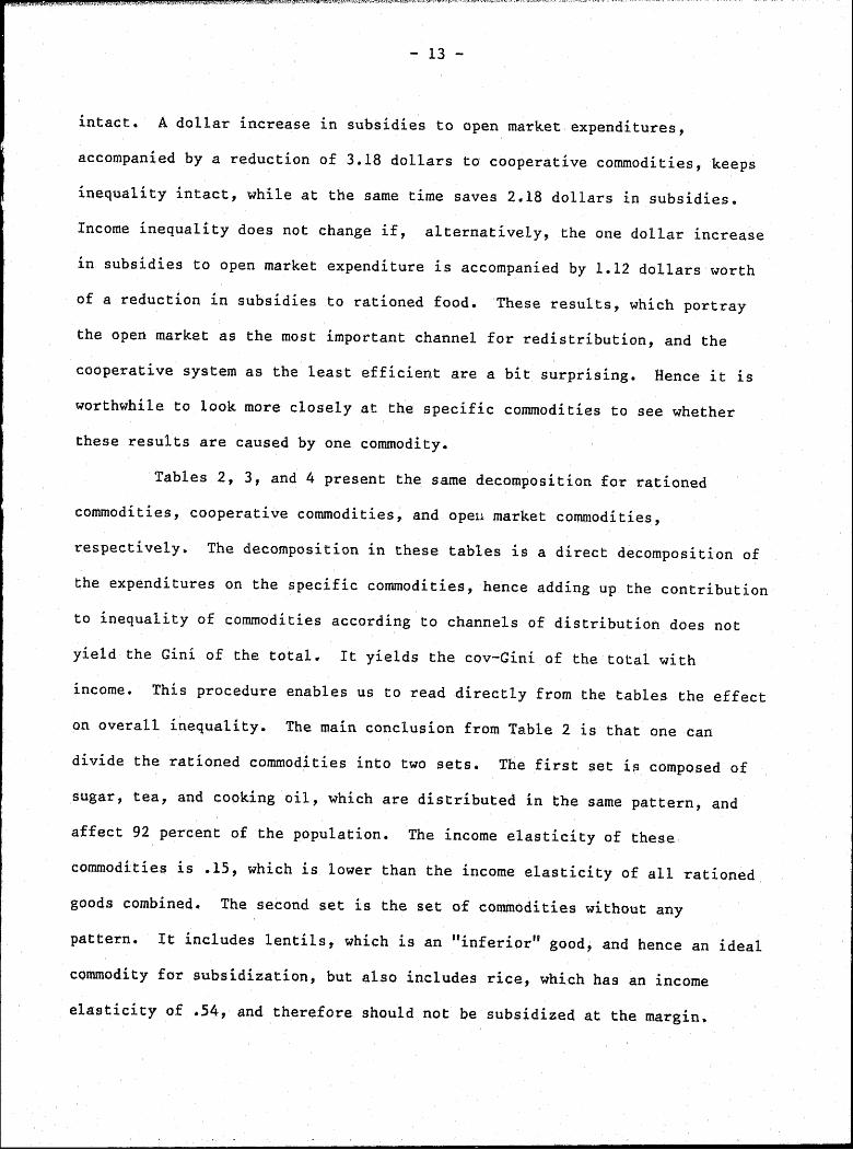
intact. A dollar increase 1n subsidies to open market expenditures,

accompanied by a reduction of 3.18 dollars to cooperative commodities, keeps

inequality intact, while at the same time saves 2.18 dollars in subsidies.

Income inequality does not change if, alternatively, the one dollar increase

in subsidies to open market expenditure is accompanied by 1.12 dollars worth

of a reduction in subsidies to rationed food. These results, which portray

the open market as the most intportant channel for redistribution, and the

cooperative system as the least efficient are a bit surprising. Hence it is

worthwhile to look more closely at the specific commodities to see whether

these results are caused by one commodity.

Tables 2, 3, and 4 present the same decomposition for rationed

commodities, cooperative commodities, and opeH market commodities,

respectively. The decomposition in these tables is a direct decomposition of

the expenditures on the specific commodities, hence adding up the contribution

to inequality of commodities according to channels of distribution does not

yield the Gini of the total~ It yields the cov-Gini of the total with

income. This procedure enables us to read directly from the tables the effect

on overall inequality. The main conclusion from Table 2 is that one can

divide the rationed commodities into two sets. The first set i~ composed of

sugar, tea, and cooking oil, which are distributed in the same pattern, and

affect 92 percent of the population. The income elasticity of these

commodities is .15, which is lower than the income elasticity of all rationed

goods combined. The second set is the set of commodities without any

pattern. It includes lentils, which is an "inferior" good, and hence an ideal

commodity for subsidization, but also includes rice, which has an income

elasticity of .54, and therefore should not be subsidized at the margin.

- 14 -

Therefore one can conclude that a reduction of the subsidy on rationed rice

will improve the performance of the rationing system.

Table 3 presents the same decomposition as before with respect to

cooperative commodities. The performance of ~11 commodities inspected is

worse than the performance of any rationed commodity. Moreover, the income

elasticity of cooperative tea is greater than one, implying that a decrease of

the subsidy on this commodity, and (for example) redistributing the money

saved by a proportional (negative) income tax decreases inequality. In other

words, eliminating the subsidy would reduce inequality. Although the results

for other commodities are not so extreme as in the case of tea, none

presents an efficient method of improving the well-being of the poor. The

justification for the cooperative system can't be based on the ground of

improving the welfare of the poor in the society.

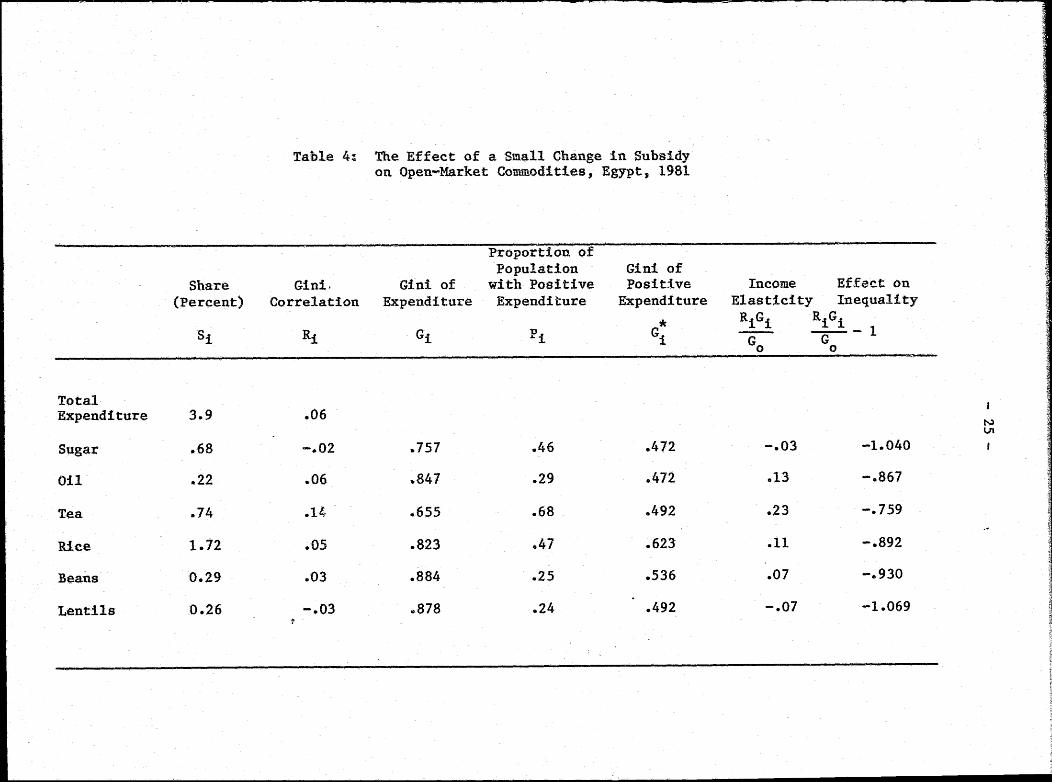
Table 4 presents the effect on inequality of open-market com­

modities. There are two inferior commodities, sugar and lentils. With the

exception of tea, all other commodities are more effective than the rationed

commodities. That is, in the case o£ sugar, cooking oil, rice, and beans, an

increase of the subsidy on the open-market commodity financed by a decrease in

the subsidy for rationed commodity decreases income inequality. However,

there is a difference in the magnitude of improvement. The most effective

subsidies are those on sugar and rice, while in the c~ses of beans and oil the

changes in inequality will be small and given that there exists a sampling

error, one can argue that although there is some improvement for beans and

oil, the improvement is not statistically significant. The mere fact that

the cooperative system and the rationing system are not performing far better

than the open market in reducing inequality hints that those systems are not

- 15 -

efficient. Note that this conclusion was reached although the administrative

aspects were ignored. Since the cost of administering the rationing and the

cooperative system are probabely higher than the cost of intervention in the

open market, a general approach which would take these costs into account

would strengthen the conclusion reached in this paper.

The ratios of the entries in the last column of tables 1-4 enable us

to estimate the revenue effect of the following exercise: Assume that the

subsidy on one commodity is increased while the subsidy on another commodity

is decreased, such that overall inequality remains intact. What is the effect

on the outlay on subsidies. For example, an increase of one dollar in the

subsidy of open market sugar, (-1.04, see table 4, line 1) and a reduction of

3.67 dollars (-1.04/-.283, see table 1, third line) in subsidies for

cooperative goods will leave inequality unaffected. This will save the

government 2.67 dollars in subsidy for each dollar of transfer.

IV. Sensitivity analysis of the main results

The use of a sum~ary measure of inequality requires, explicitly or

implicitly, assumptions on distributional weights. At the same time, one can

argue that behind any social policy there exist distributional weights. If

these two sets of distrib~tional weights happened to be the same, then the

analysis based on the aggregate measure is meaningful. Otherwise the results

may simply reflect the difference between the assumptions of the investigator

and the preferences of the policy makers.

The use of the Gini coefficient as a measure of inequality is no

exception. Therefore it is worth trying to see whether our conclusions would

- 16 -

change if we would have used other distributional weights to evaluate the

distributional impact of subsidies.

The extended Gini offers a variety of distributional weights,

depending on the parameter v. The regular Gini is a special case where v=2.

The higher 1s v, the higher is the weight given to the lower income groups,

and in the extreme case where v+oo then the extended Gini ·represents the

attitude toward inequality as viewed by the Rawlsian criteria. On the other

hand when v+l then the extended Gini represents indifference to inequality.

Since the indices are similar, the analysis proceeds in a similar manner as

above. In order to concentrate on the main points, Table 5 presents only the

elasticities of the three main categories of commodities, estimated by using

different parameters of v. As can be seen the income elasticity of rationed

commodities declines with v while the income elasticity of open market

commodities increases with v. This means that the more we care about the

welfare of the poor, the more important are rationed commodities relative to

open market commodities. When v is greater than 5, then the income elasticity

of open markets commodities becomes higher than the income elasticity of

rationed commodities, meaning that an increase in the subsidies to rationed

food financed by an increase of the taxes on open market commodities decreases

inequality. This conclusion is in contrast with the conclusion that we

reached in the previous section, when the standard Gini was used to

characterize the distributional weights.. Therefore, it may be that the

explanation for our results in the previous section is due to misrepresent­

ation of the preference of the decision-makers regarding the welfare of the

poor in Egypt.

- 17 -

Unlike the case of rationed commodities where no clear cut conclusion

can be reached, the case of cooperative commodities offers a clear

conclusion. Income elasticities of cooperative commodities do not portray a

monotonic relationship with v, which means that the beneficiaries from

subsidies on these commodities are scattered along the income distribution.

Under all weighting schemes examined, the income elasticity of cooperative

commodities is higher than the income elasticities of open market or rationed

goods. Therefore we can conclude that the decrease of subsidies on

cooperative commodities, combined with a compensation of smaller amount by an

increase in subsidies to open market or rationed goods, can preserve

inequality and decrease the deficit in the budget.

An alternative way of examining the sensitivity of our conclusions to

alternative weighting schemes,is to ask whether there exists an additive

social welfare function, with non-negative and declining marginal utility,

that can negate our conclusions. One way of answering such a question is to

utilize a methodology that was developed in Yitzhaki and Slemrod (1987) and is

referred to as marginal conditional stochastic dominance. The p~ocedure is

based on the following proposition:

Consider a (small) increase in the subsidy for commodity A that is financed by

an increase in the tax on commodity B, such that the tax revenue does not

change. Then a necessary and sufficient condition for all additive welfare

functions to show an increase in social welfare is that the concentration

curve of commodity A is always above the concentration curve of commodity

B. 12/

Our intention is to use this proposition in order to see whether it

is possible to find out a social welfare function that can justify subsidies

- 18 -

to the cooperative system~ Before we proceed it is worth mentioning that this

is an extreme test, in the sense that in each comparison we allow a different

welfare function to be used. That is, it is possible that we justify the

subsidy on cooperative commodities by using one welfare function, and later

justify the subsidy on rationed goods by another welfare function.

Figure 1 presents the Difference in concentration curves (hereafter,

DCC curve) between open market commodities and rationed Goods. On the

horizontal axis is the cumulative distribution of the population, ordered

according to income per capita. On the vertical axis the DCC curve is

plotted. The DCC curve is the vertical difference between the concentration

curve of open market commodities and the concentration curve of rationed

commodities. If the DCC curve does not intersect the horizontal axis, it

means that the concentration curve of open market commodities is always above

the concentration curve of rationed goods. As can be seen from Figure 1, The

DCC curve intersects the horizontal axis from below, which means that there

exists a welfare function for which the increase in the welfare of the lowest

two deciles of the income distribution can justify an increas€ in the subsidy

in rationed good financed by a tax on the open market goods. This confirms

the conclusions that we reached by using the extended Gini.

Figure 2 presents the DCC curve of open market commodities minus

cooperative goods. As can be seen, the curve intersects the horizontal axis

in several places in the lowest decile. This implies that one can find a

social welfare function which will not justify the cut in subsidies to

cooperative commodities and transfer of the proceeds to subsidize open market

commodities. However, since the curve is negative for only 12 observations it

may be that this result is due to sampling error.

- 19 -

Figure 3 presents the DCC curve of rationed commodities minus

cooperative commodities. As can be seen, the curve does not intersect the

horizontal axis, which means that all additive social welfare functions will

show that an increase of the subsidy on rationed commodities financed by a

reduction in the subsidies for cooperative commodities increases welfare.

Hence we may conclude that it is impossible to find a welfare function that

will not justify a reduction in the subsidy fo~ cooperative commodities- If

there is an argument for subsidizing cooperative goods at the present rate, it

cannot be based on distributional ground~

V. The distributional effect according to regions

Lipton (1979) alerted economists to the urban bias in many developing

countries policy making. Although we are tempted to agree with Lipton that

the urban bias is unjustified, one may also argue that the economist, whose

role is to advise the government, should respect the preferences of the

decision makers. To the best of my knowledge, no one has proposed a formal

social welfare function with an ·urban bias. However, if we believe that there

is an urban bias, and that economists should respect the preferences of the

decision makers, then we have to account for an urban bias in the preferences

of governments, whatever its origin. The methodology presented here is

flexible enough to account for an urban bias. To illustrate this, we analyze

an extreme case where the government cares only about redistribution in the

urban sector. lJ/ Does this radical change in preferences forces a change in

the conclusions reached above?

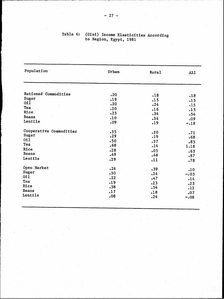
The policy recommendations depend on one parameter, the income

elasticity o£ the commodity. Table 6 presents the income elasiticities of all

- 20 -

commodities for the urban and rural populations, using the weighting scheme of

the Gini coefficient. Surprisingly, for almost all the commodities, the

income elasticity for the whole economy is totally different than the income

elasticities of the urban or the rural populations. Since no restrictions

were imposed on the curvature of the Engel curves, such deviations may occur

because of the differences between the two populations. The mean income per

capita of the urban population is 1.8 times the mean income per capita of the

rural population. Hence in many cases when the income elasticity of the urban

population is lower than the income elasticity of the rural population, the

overall elasticity, which takes into account the difference between the rural

and urban populations, tends to be lower than both the elasticities of the

rural and urban populations. l4/

The case of cooperative commodities is a typical example that is

worth examining. The income elasticity of these commoditie::; for the urban

population is .35 which is higher than the income elasticity for the rural

population (.20). The income elasticity for the whole population is .71.

Therefore, it is the difference between the rural and urban populations that

~aused us to conclude that the cooperative system is inefficient on the

margin. A similar situation, although in reverse direction is the case of

open market commodities. Since the income elasticity for rural population is

higher than the income elasticity for urban population, the overall elasticity

is smaller than both elasticities, which explains the importance of the open

mar:ket commodities for redistribution through taxation. The rationed

commodities have similar elasticities for both populations, and a similar

income elasticities for the overall population. Hence the redistributional

effect of these commodities is not affected by the choice of population.

- 21 -

The conclusion from the above discussion is that the ranking of

I commodities according to their effectiveness as instruments for

redistributions depends crucially on the target population. If we care only

on redistribution in the urban population, then the rationed commodities are

the most efficient instrument, the open markret is less effective, while the

cooperative system is the least important. However, the differences in th~

performances of the different commodities are less dramatic than in the cas.e

where the target population is all Egypt. In the last case th.e most effective

channel for redistribution is the open market and the ineffectiveness of the

cooperative commodities 'is much more pronounced. Therefore, the conclusion

that a reduction in the subsidies to cooperative commodities accompanied by an

increase in the subsidies to either the open market or the rationed

commodities can decrease the deficit in the budget and at the same time does

not deteriorate the redistributional impact of the subsidy system, remains

intact.

Share (Percent)

si

Total Expenditure 26.90 a/

Expenditure on:

Rationed Food 2.3

Cooperative 0.5

Free Market 3.9

Other Expenditure 93.4

Gini

Table 1: The Effect of a Small Change in Subsidies On Inequality, Egypt, 1981

Proportion ¢f Population Gini of

Gini of with Positive Positive Correlation Expenditure Expenditure Expenditure

Ri Gi pi * Gi

.381

.17 .400 .92 .348

.35 .780 .41 .463

.06 .636 .84 .567

.99 .405

a. Mean income per capita, Egyptian Lira, 1981.

Income Effect on Elasticity Inequality RiGi RiGi

--1 Go G

0

"'-> t-.)

el8 -.822

.71 -.283

.10 -.900

Share (Percent)

si

Total Expenditure 2.3

Sugar 1.0

Oil 0.4

Tea 0.6

Rice 0.2

Beans 0.04

Lentils 0.05

Table 2: The Effect of a Small Change in Subsidies on Rationed Commodities, Egypt, 1981

Proportion of Population Gini of

Gini Gini of with Positive Positive Correlation Expenditure Expenditure Expenditure

* Ri Gi pi Gi

.17

.14 .416 .92 .365

.13 .444 .92 .396

.14 .416 .92 .365

.34 .604 .84 .529

.05 .. 692 .47 .345

-.11 .657 .53 .353

Income Effect on Elasticity Inequality

RiGi RiGi --1

G G 0 0

.15 -.847 N w

.15 -.849

.15 -.847

.54 -.461

.09 -.909

-.18 -1.190

Share (Percent)

si

Total Expenditure o.so

Sugar 0.28

Oil 0.09

Tea 0.02

Rice 0.08

/ ' Beans o.o1

Lentils 0.05

Table 3: The Effect of a Small Change in Subsidies on Cooperative Commodities, Egypt, 1981

Proportion of Population Gini of

Gini Gini of with Positive Positive Correlation Expenditure Expenditure Expenditure

* Ri Gi pi Gi

.35 .,.

.32 .809 .32 .403

.35 .899 .17 .IJ06

.46 .979 .f)] .70

.26 .920 .14 .428

.34 .973 ,04 .325

.32 .941 .10 .410

Income Effect on Elal'tticdty Inequality

Ri(..:i RiGi --1

Go G 0

.71

.68 -.321 N ~

.. 83 -.174

1.18 .182

.63 -.372

.87 -.132

.79 -.210

Share (Percent)

si

Total Expenditure 3.9

Sugar .68

Oil .22

Tea .74

Rice 1.72

Beans 0.29

Lentils 0.26

Table 4: The Effect of a Small Change in Subsidy on Open-Market Commodities, Egypt, 1981

Proportion. of Population Gini of

Gini. Gini of with Positive Positive Correlation Expenditure Expenditure Expenditure

* Ri Gr pi Gi

.06

-.02 .757 .46 .472

.06 .847 .29 .472

.ll~ .655 .68 .492

.05 .823 .47 .623

.03 .884 .25 .536

-.03 01878 .24 .492 'l"

Income Effect on Elasticity Inequality

RiGi RiGi ----1

Go G 0

N VI

-.03 -1.040

.13 -.867

.23 -.759

.11 -.892

.07 -.930

-.07 -1.069

Gini Parameter

Commodities

Rationed Commodities

Cooperative Commodities

Open Market Commodities

- 26 -

Table 5: Income Elasticities According to Different Weighting Schemes

v = 1.5 2.0 3.0 4.0

.179 .178 .177 .172

.684 .717 .741 .731

.077 .100 .126 .159

10.0

.168 .146

.718 .658

.174 .241

- 27 -

Table 6: (Gini) Income Elasticities According to Region, Egypt, 1981

Population Urban Rural

Rationed Commodities .20 .18 Sugar .19 .15 Oil .. 20 .24 Tea .20 .16 Rice .25 .34 Beans elO .34 Lentils .09 .19

Cooperative Comm.oditie~ .35 .20 Sugar .29 .19 Oil .so .37 Tea .68 .14 Rice .28 .os Beans .49 .48 Lentils .29 .11

Open Market .26 .39 Sugar .30 .24 Oil .22 .47 Tea .19 .23 Rice .38 .54 Beans .17 .18 Lentils .08 .24

All

.18

.15

.15

.15

.54

.09 -.18

.71

.68

.83 1.18

.63

.. 87

.78

.10 -.03

.11-f.

.23

.12

.07 -.08

Difference in

0 .. 05 ..,.

concentration curves

0.04

0.0~

0.02

0.01

0

.. 0.01

1 I f I I j

I f

•·i 1

I I t f

l

. I I I {

I

Figure 1: The Difference Between the Concentration Curves of Open Market and Rationed Commodities

··-·- .. ~ -- .. , l l !

. 0.02 ["-· -, .. - -~- .. ..,.-.-.. -----~· ··r-- .... ,----..-·-:··-·#r ........ _ --..... _ ."_ ... __ ·-·.,··~-- ...... ; -· ·--· .. --"" ·-T i

·~·---- ~r ... -, .. --.~--, .. ·;·· · ~······---·· ... r··--·- ··-·--t

0 0.2 0.4· 0.6

Cumulative Distribution of Population According to Per Capita Income

0.8

N 00

..

Difference 0.22 in Concentration O

2 Curves ..

0.1 a

0.16

0.14

0.12 -

0. t ~

0.08

0 .. 06

0.04 ..

0.02

0

Figure 2: The Difference Between the Concentration Curves of Open Hark.et and Cooperative Commodities

. ·····~-- .. -- . ----~~·~- . ~··· -·--·~---···---··--· ·-·-----· -· ----·~-·-·--·---· ~ "·--·-----·--··--- --··1

,,~, c ~- ·--·-----·----· ------~------·-.·---------·

M

~

\ I ·. ·-----····--·--~

I I

- 0. 02 -·: -r-----,----. --....,._.--,------r-----r------1

0 0.2 0.4 0.6 0,8 1

Cumulative Distribution of Population According to Per Capita Income

N \0

I

0.01 l

Figure 3:. The Difference Between the Concentration Curves of Rationed Commodities and Cooperative Commodities

0 """·;-·--·"-·,.--v-,.a·-·-.. · 4 ·~·--·----·- ..... .._ .. -;- ...... -------·-·-~··----·--· ..... ________ r....,...._·--~---T---- ... -;,.-·---.. -i _____ .,. __ !.

0.2 0~4 0.6

Cumulative Distribution of Population According to Per Capita Income

0.8 1

- 31 -

Endnotes

* The cooperation of Harold Alderman in providing the 1981 Egyptian Survey

and generously sharing his knowledge of the data set is gratefully

acknowledged. I would also like to thank Joel Slemrod for his comments on

an earlier draft and Reza Firuzabadi for research assistance.

1. For an excellent review and description of the rationing system in Egypt,

see Alderman, Von Braun 1 and Sakr (1982).

2. See Michael Lipton (1979) for a critial view.

3. See Alderman, Von Braun and Sakr (1982) for a detailed description of the

system, and Alderman and Von Braun (1984,1986) for an analysis using

conventional methods.

4. When dealing with rationed and cooperative commodities, the consumer is

not free to choose the quantities, hence the meaning of an inferior good

is that the marginal eligibility to receive to commodity is negative.

5. In the case of the extended Gini then the extended Gini correlation is

defined as cov(xi,[l-Fy(y)]v-1)/ cov(xi,[l-Fi(xi)]v-l). Properties a,b

and c hold in this case too, See Stark, Taylor and Yitzhaki (1987)]

6. Note that the share and the Gini correlation can be negative (e.g. taxes).

7. Note, however, that one way to introduce efficiency considerations into

..: - 32 -

the analysis, is to take into account only the change that will keep the

consumer at the same utility level. In this case the higher the

compensated elasticity of demand; the lower the compensation needed.

8. In the case of the extended Gini the weights will be:

In this case the weight function is asymmetric and the weights given to

the marginal propensity to spend of low income groups are an increasing

function of v.

9. Unfortunately, we don't have reliable data on specific items of bread and

energy, which are major targets for heavy subsidization.

10. For a description of the samples, see Alderman and Von Braun (1984). {The

urban population is assumed to be 44 percent of the overall population.)

11. Income is defined as total expenditure per capita per year.

12. The concentration curve ~C(F) describes the percentage of overall

expenditure on commodity C that is spent by the poorest F families. Its

properties are discussed in Kakwani (1980), Nygard and Sandstrom (1981)

and Yitzhaki and Olkin (1987).

- 33 -

13. It is assumed that the urban bias means that the government ignores the

rural population. An alternative assumption is that the government tax

the rural sector and transfers the proceeds to the urban sector. This

possibility is ignored.

14. It is worth noting that the urban bias in subsidies in Egypt was detected

by Alderman, Von Braun and Saker {1982) who used a conventional regression

technique. Hence, the findings with regard to the urban bias are not

related to the technicque used in this paper.

- 34-

References

Alderman, Harold and Joachim Von Braun {1984) *'The Effects of The Egyptian

Food Ration and Subsidy System on Income Distribution and Consumption",

International Food Policy Research Institute, Research Report No. 45,

(July)

Alderman, Harold and Joachim Von Braun {1986). "Egypt's Food Subsidy Policy:

Lessons and Options", Food Policy 11, No. 3, (August)

Alderman, Harold, Joachim Von Braun and Sakr Ahmed Sakr (1982) "Egypt Food

Subsidy and Rationing System: A Description.'' International Food Policy

Research Institute, Research Report No. 34, (October)

Lipton, Michael (1977) Why Poor People Stay Poor, A Study of Urban Bias in

World Development, Australian National University Press, Temple Smith,

London.

Lerman, Robert, and Shlomo Yitzhaki (1984) "A Note on the Calculation ad the

Interpretation of the Gini Index," Economics Letters, No. 15.

Kakwani, Nanak C. (1980) Income Inequality and Poverty: Method of Estimation

and Policy Applications. New York: Oxford University Press.

Nygard, Fredrik and Arne Sandstrom (1981) Measuring Income Inequalitz.

Stockholm: Almqrist and Wiksell International.

- 35 -

Sadiq, Ahmed (1984) "Public Finance in Egypt 1 " World Bctnk Staff Working Paper,

No. 639, Washington.

Schechtman, Edna, and Shlomo Yitzhaki (1987) ''A Measure of Association based

on Gini's Mean Difference," Communication in Statistics, Theory and

Methods, Al6, No. 1, January.

Sievers, Gerald L. (1978) "Weighted Rank Statistics for Simple Linear

Regression," Journal of the American Statistical Association, Theory and

Method Section, 363, September.

Stark, 0 .. , J. E. Taylor, and s. Yitzhaki (1986) "Remittances and Inequality,"

The Economic Journal 96, September, 722-740.

Stark, o., J. E. Taylor and S. Yitzhaki (1987) uMigration, Remittances and

Inequality: A Sensitivity Analysis Using The Extended Gini Index," Journal

of Development Economics, forthcoming.

Yitzhaki, Shlomo (1973) "On An Extension of Gini Inequality Index,~'

International Economic Review, 94, No. 3, October ..

Yitzhaki, Shlomo (1986) non the Progressivity of Commodity Taxation,u

Development Research Department Discussion Paper No. 255, The World Bank,

December.

- 36 -

Yitzhaki, Shlomo, and Joel Slemrod (1987) uon Welfare Dominance: An

Application to Commodity Taxation," Provisional Papers in Public Economics

No, 87-9, The World Bank, April.

Yitzhaki, Shlomo and Ingram Olkin (1987) "Concentration Curves," Technical

Report No. 230, Department of Statistics, Stanford University, April.

Some Recent DRD Discussion Papers

273. Growth and Structural Change in East Africa: Domestic Policies, Agricultural Performance and World Bank Assistance, 1963-1986, Part I, by U. Lele and R. Meyers.

274. Growth and Structural Change in East Africa: Domestic Policies, Agricultural P~rformance and World Bank Assistance, 1963-196, Part II, by u. Lele and R. Meyers.

275. Abstracts of Development Research Department Publications: April 1986 -April 1987.

276. Korea's Hacroeconomic Prospects and Major Policy Issues for the Next Decade, by V. Corbo and S.W. Nam.

277. The Pricing of Manufactured Goods During Trade Liberalization: Evidence from Chile, Israel, and Korea, by V. Corbo and P.D. McNelis.

278. :Fiscal Policy and Development Strategy in Southern Asia, by G .• F. Papanek,.

279. Evolution of the Tunisian Labor Market, by c. Morrisson.

280. Labour Allocation Across Labour Markets Under Different Informational Schemes and the Costs and Benefits of Signalling, by 0. Stark and E. Katz.

281. Mobility, Skill and Information, by o •. Stark and E. Katz.

282. Labour Mobility and Intrafamilial Income Transfers: Theory and Evidence from Botswana, by 0. Stark and R. Lucas.

283. Labour Migration, Income Inequality and Remittances: A Case Study of Mexico, by 0. Stark, J.E. Taylor and S. Yitzhaki.

284. Female Labour Mobility, Skill Acquisition and Choice of Labour Markets; Theory and Evidence from the Philippines, by 0. Stark and J. Lauby.

285. Market Structure, Jobs, and Productivity: Observations from Jamaica, by P.B. Doeringer.

286. Coordination of Taxes on Capital Income in Developing Countries, by P.B. Musgrave.

287. The Effects of Labor Regulation Upon Industrial Employment in India, by P.R. Fallon.

288. Factor Substituion in Production in Industrialized and Less Developed Countries, by D. Demekas and R. Klinov.