c_ ie,5u_ I I o-f

CSDL-T-1083

MULTIVARIABLE CONTROL OF THESPACE SHUTrLE REMOTE

MANIPULATOR SYSTEM USING

H2 AND H_ OPTIMIZATION

byOm Prakash II

May 1991

Master of Science Thell$Mamchuuttl Institute of Technology

[f!__ 5_,kCL _!JOT[LL _F_!-_F_: _A_;IDULAT/_ SYST_::M

USi_!(, <_ ^_r_ !_(INFINITY) c_PTIMIZATI_N M.S.

thesis - _<_ssachusetts Inst. of l_:_.ch.

(mr_F,r (CCIIFI ;S St._rk) L.:_.t).) ]1 _ oCSCL 1-_[_I_

DRAPERThe Charles Stark Draper Laboratory, Inc.

555 Technology Square, Cambridge, Massachusetts 02139-3563

https://ntrs.nasa.gov/search.jsp?R=19910018226 2018-06-12T18:18:43+00:00Z

Multivariable Control of the

Space Shuttle Remote Manipulator System

Using H2 and Ha Optimization

by

Om Prakash II

B.S., Engineering Sciences,

United States Air Force Academy

(1989)

SUBMITTED TO THE DEPARTMENT OF AERONAUTICS AND

ASTRONAUTICS IN PARTIAL FULFILLMENT OF THE

REQUIRMENTS FOR THE DEGREE OF

MASTER OF SCIENCE

at the

MASSACHUSETTS INSTITUTE OF TECHNOLOGY

May, 1991

© Om Prakash II, 1991. All rights reserved.

Signature of Author

Certified by

Certified by

Department of Aeronai_tics and Astronautics

May, 1991

Technical Staff, C. S. Draper Labs

Technical Supervisor

Wallace E. VanderVelde

Professor of Aeronautics and Astronautics

Thesis Supervisor

Accepted by

Professor Harold Y. Wachman

Chairman, Departmental Graduate Committee

Multivariable Control of the

Space Shuttle Remote Manipulator System

Using H2 and H_o Optimization

by

Om Prakash II

Submitted to the Department of Aeronautics and

Astronautics on May 10, 1991 in partial fulfillment of the

requirements for the degree of Master of Science

Abstract

Three linear controllers are designed to regulate the end effector of the Space Shuttle Remote

Manipulator System (SttMS) operating in Position Hold Mode. In this mode of operation, jet

firings of the Orbiter can be treated as disturbances while the controller tries to keep the

end effector stationary in an Orbiter-fixed reference frame. The three design techniques used

include: the Linear Quadratic Regulator (LQR), H2 optimization, and H¢o optimization.

The nonlinear SRMS is linearized by modelling the effects of the significant nonlinearities

as uncertain parameters. Each regulator design is evaluated for robust stability in light of the

parametric uncertainties using both the small gain theorem with an Hoo norm and the less

conservative #-analysis test.

All three regulator designs offer significant improvement over the current system on the

nominal plant. Unfortunately, even after dropping performance requirements and designing

exclusively for robust stability, robust stability cannot be achieved. The SRMS suffers from

lightly damped poles with real parametric uncertainties. Such a system renders the #-analysis

test, which allows for complex perturbations, too conservative.

Technical Supervisor:

Thesis Supervisor:

Nell J. Adams

Technical Staff, Manned Space Systems Division,

The Charles Stark Draper Laboratory, Inc.

Dr. Wallace E. VanderVelde

Professor of Aeronautics and Astronautics

f_1_d_t&l_.N L'ON¢dJ._f_M

3

PRECEDING PAGE BLANK NOT FILMED

Acknowledge me nts

An ocean of patience, a mountain of insight,

Captains a craft through the storm, guides the ornithopter through the night.

The chaos of my thoughts you ordered with ease,

And extracted a thesis as effortless as a breeze.

Neil I am grateful and in your debt will always be,

And I truly understand why you're the star of EGC.

Amazed at the circus, my mouth open wide,

As the trapeze artist casts gravity aside,

And the great Nabakov with his mastery of words,

Or the mighty strokes of Mozart as he conjures the chords.The hard work and dedication that these Masters represent,

Is personified in Controls by the Oracle, or Brent.

Take the legendary Conan and a Trumpful of greed,

Be liberal with cynicism, and some virtuosity youll need.

Combine all of these things with generous portions of heart,

And you'll come up with Naz, at least in part.

Thanks Professor VanderVelde for your careful reading and valuable suggestions,

And Don's 'divide by 12' answered many of my questions.

Dave I reserve a special place for you,

Full of honest ideals and compassion too.

So don't harass my friend or get on his case,

Dave knows it's not the kill, but the thrill of the chase.

Though you may not realize, I know to be true,

That the Odyssey is about Scott, and the Illiad too.

But I hope you remember even Odysseus came back,

And scattered the suitors by piercing many an ax.

Ching, Bill, Karl, Noel, Kris and Steve,

From your company I sadly take my leave:

"HOTMOKD SD, WJ GO KOSRLAYTY NOWJ SR KOSD."

Answers in seclusion have insignificant tangible extensions,

Resist until you understand mankinds' intentions.

From my parents flows my body, and from Dharma my mind,

Though it is western religions that put time on a line,

So to express my gratitude during this short sojourn on Earth,

I try to apply my abilities to the best of their worth.

5

PRE'CEDiI",]G PAGE BLANK NOT FILMED

This report was prepared at the Charles Stark Draper Laboratory, Inc. under contractNAS9-18147.

Publication of this report does not constitute approval by the Draper Laboratory or the

sponsoring agency of the findings or conclusions contained herein. It is published solely for the

exchange and simulation of ideas.

I hereby assign my copyright of this thesis to the Charles Stark Draper Laboratory, Inc.,

Cambridge, Massachusetts.

6

Contents

1 Introduction 13

4

Description of the Shuttle Remote Manipulator System 18

2.1 Physical Description .................................. 19

2.2 SRMS Control Modes ................................. 21

2.3 Position Hold ...................................... 22

Modelling the SRMS 25

3.1 Equations of Motion'for the Orbiter/SRMS/Payioad System ........... 27

3.1.1 Equations of Motion for the Single Joint Case ................ 27

3.1.2 Equations of Motion for the Six Joint Case ................. 30

3.2 Modelling and Linearization of the Control Servos ................. 32

3.2.1 Control Servo Dynamics ............................ 32

3.2.2 Representing the Uncertainties ........................ 37

3.3 Comparison of the Linear and Nonlinear Plant ................... 42

3.4 Conclusions ....................................... 46

Design and Analysis Approach 49

4.1 Obtaining a Design Plant ............................... 50

4.1.1 Model Reduction ................................ 52

4.1.2 Characteristics of the ROM .......................... 54

4.2 Analysis Techniques and the Open-Loop Plant ................... 57

4.2.1 Performance .................................. 59

4.2.2 Control Effort .................................. 59

?

4.2.3 Stability Robustness .............................. 61

4.3 Summary ........................................ 68

5 LQR Design 69

5.1 LQR Theory ...................................... 69

5.2 LQR Results ...................................... 72

5.2.1 LQR Control Effortand Performance .................... 72

5.2.2 LQR StabilityRobustness ........................... 77

5.3 Summary ........................................ 79

6 //2 Design 80

6.1 /-/2Theory ....................................... 81

6.2 //2 Results ....................................... 86

6.2.1 H2 Control Effortand Performance ...................... 86

6.2.2 /-/2StabilityRobustness ............................ 89

6.3 Summary ........................................ 95

7 Hoo Design 96

7.1 Hoo Theory ....................................... 97

7.2 Hoo Results ....................................... 100

7.2.1 Hoo Control Effort and Performance ..................... 100

7.2.2 Hoo Stability Robustness ........................... 104

7.3 Summary ........................................ 115

8 Conclusions 116

List of Figures

1.1 Cumulative SRMS Damping Time .......................... 14

2.1 Shuttle Remote Manipulator System ......................... 19

2.2 Mechanical Arm Assembly ............................... 20

2.3 Typical SRMS Maneuver Profile ........................... 23

3.1 Block Diagram of the Compensated System ..................... 26

3.2 One Joint Illustration: Point Mass on a Massless Flexible Beam .......... 28

3.3 Draper Servo Model .................................. 33

3.4 Linearized Servo Model ................................ 35

3.5 Linearized SRMS Model ................................ 36

3.6 Gearbox Stiffness Curve ................................ 38

3.7 Current Limiter ..................................... 39

3.8 Standard Form for a Compensated Plant with Uncertainty ............. 41

3.9 SSAD in Position Hold ................................. 43

3.10 Translation Response of LSAD and Nominal SSAD to an Initial Velocity ..... 44

3.11 Rotational Response of LSAD and Nominal SSAD to an Initial Velocity ..... 45

3.12 Translation Response of LSAD and off-nominal SSAD to an Initial Velocity . . . 47

3.13 Rotational Response of LSAD and off-nominal SSAD to an Initial Velocity . . . 48

4.1 Poles of Open-Loop SSAD ............................... 51

4.2 Poles of the Position Hold Open-Loop SSAD .................... 53

4.3 Singular Values from Joint Rate Commands to End Effector State for the ROM

and FOM ........................................ 55

4.4 Poles of the Reduced Order Model .......................... 56

4.5

4.6

4.7

4.8

4.9

4.10

4.11

4.12

Transmission Zeros of the Reduced Order Model .................. 56

Performance Singular Values of the Current Position Hold System ........ 60

Control Effort Singular Values of the Current Position Hold System ....... 62

Closed-Loop Transfer Function ............................ 62

Closed-Loop System for Robust Stability Analysis ................. 63

Robust Stability Analysis of the Current Position Hold System .......... 66

Open-Loop System Near Pole Locations With K¢; = 0.01 and K_tA = K_¢a,,4, • 67

Open-Loop System Near Pole Locations With K¢i = 0.05 and Kt,_A = K_¢A,=,,= . 68

5.1 Plant With.Compensator ............................... 70

5.2 Control Effort Singular Values of the LQR System ................. 73

5.3 Performance Singular Values of the LQR System .................. 74

5.4 Translational Response of PH System and LQR System to Attitude Thruster

Commands ....................................... 75

5.5 Rotational Response of PH System and LQR System to Attitude Thruster Com-

mands .......................................... 76

5.6 Robust Stability Analysis of the LQR System .................... 77

5.7 LQR Closed-Loop System Near Pole Locations for the Nominal and Off-Nominal

System ......................................... 78

6.1 Plant With Compensator ............................... 81

6.2 Control Effort Singular Values of the H2 System .................. 87

6.3 Performance Singular Values of the H2 System ................... 88

6.4 Translational Response of PH System and//2 System to Attitude Thruster Com-

mands .......................................... 90

6.5 Rotational Response of PH System and H2 System to Attitude Thruster Com-

mands .......................................... 91

6.6 Robust Stability Analysis of the H2 System ..................... 92

6.7 Closed-Loop Poles of the Nominal H2 System .................... 92

6.8 Closed-Loop Poles of the Off-Nominal H2 System: 1 ................ 93

6.9 Closed-Loop Poles of the Off-Nominal //2 System: 2 ................ 93

6.10 Closed-Loop Poles of the Off-Nominal//2 System: 3 ................ 94

10

6.11 Closed-Loop Poles of the Off-NominM H2 System: 4 ................ 94

7.1

7.2

7.3

7.4

7.5

7.6

7.7

7.8

7.9

7.10

7.11

7.12

7.13

7.14

7.15

7.16

7.17

Plant With Compensator ............................... 97

Control Effort Singular Values of the H_ System .................. 101

Performance Singular Values of the Hoo and Position Hold Systems ........ 102

Performance Singular Values of the Hoo and/-/2 Systems .............. 103

Translational Response of Pil,/-/2, and Ho_ Systems to Attitude Thruster Com-

mands .......................................... 105

Rotational Response of Pil, H2, and H_ Systems to Attitude Thruster Commands l06

Robust Stability Analysis of the Hoo System .................... 107

Closed-Loop Poles of the Nominal Hoo System ................... 108

Closed-Loop Poles of the Off-Nominal Hoo System: 1 ................ 108

Closed-Loop Poles of the Off-Nominal H_ System: 2 ................ 109

Closed-Loop Poles of the Off-Nominal Ho_ System: 3 ................ 109

Closed-Loop Poles of the Off-Nominal Hoo System: 4 ................ 110

Standard Form for a Compensated Plant with Uncertainty ............. 111

Closed-Loop Transfer Function ............................ 111

Robust Stability Analysis of the 'Gl1' Hoo System ................. 113

Control Effort Singular Values of the 'G11' H_ System .............. 113

Performance Singular Values of the 'Gl1' H_ System ............... 114

11

List of Tables

3.1 Variable Notation for One Joint EOM ........................ 28

3.2 Variable Notation for Six Joint EOM ......................... 30

3.3 Variable Notation for Servo Parameters ....................... 34

4.1 Gramian Singular Values ................................ 58

4.2 Joint Rate Limits .................................... 61

12

Chapter 1

Introduction

Future Space Shuttle operations include the on-orbit assembly of the Space Station Freedom

(SSF). This assembly process will require the Shuttle R,emote Manipulator System (SRMS) to

manipulate many separate elements of the SSF toward its ultimate construction. Experience in

SRMS payload operations gained over the last decade indicate deficiencies in current operations.

Some of these deficiencies are of particular concern for the assembly of the SSF. One such

concern is the long durations of time required to damp vibrations of the SRMS and attached

payload after a given maneuver. Attitude thruster firings of the Shuttle Flight Control System

(SFCS) during SRMS operations is another source of undesired excitations. The time spent

waiting for these undesired vibrations to damp out can consume a significant fraction of the

total mission time. For example, the estimated time spent waiting for the SR.MS to damp during

the first sixteen Shuttle flights required for the SSF assembly task is illustrated in Figure 1.1 [1].

The SRMS consists of six joints connected via tubular structural members with a grapple

at the end effector for grasping payloads. Some of these structural members are longer than

6 meters. The total length of the extended arm is over 15 meters, making for a very flexible

structure. Control of the arm is performed by six motor rate feedback servos, one for each joint.

In order to perform end effector or payload maneuvers, the SRMS has five modes of operation.

These modes include the Automatic Mode, the Manual Augmented Mode, the Single Joint

Mode, the Direct Drive Mode, and the Backup Drive Mode. The Direct Drive Mode and the

Backup Drive Mode are both contingency modes that allow the SRMS to operate even if certain

system failures occur. After the SRMS completes a maneuver in one of the three regular modes,

each servo is initially given a zero rate command. After the zero rate command state, the SRMS

13

RHS

t_ne,hours

6F5

4

3

2

1

0

[--]-RH$ settling time

1 2 3 4 5 6 7 8 9 10111213141516

Flight nomber

Figure 1.1. Cumulative SRMS Damping Time

drops into Position Hold. In Position Hold, as the name implies, the system tries to maintain

its final end-point position and attitude. The design philosophy for the SRMS is discussed in

detail by Ravindran [2].

Currently, the SRMS maintains Position Hold end-point control using the joint control

servos. In Position Hold, each joint is equipped with a controller that supplies joint rate

commands based upon angle feedback from joint encoders. However, since boom flexibility

is not observable in the joint angle feedback measurements, no active vibration suppression

currently exists for control of the SRMS and attached payload. Simple movements of the SRMS

with a heavy payload attached can cause vibration of the arm with frequencies inside the control

bandwidth. An even larger source of excitation is Shuttle attitude control thruster firings that

are required to support payload operation constraints such as: lighting, contamination, and

release or tip-off requirements. The system must wait for these vibrations to die out since it is

not actively damping them. Current control system design technology offers the opportunity

to design controllers that will actively damp such undesired vibrations. The key is to provide

such controllers with information about the structural flexibility of the SRMS.

Gilbert, et al. [1] investigated active damping of the SR,MS using a Linear Quadratic Gaus-

sian (LQG) controller. Gilbert approached the problem by replacing the zero rate command

state with a LQG controller after the SR,MS finishes a maneuver. Assuming linear accelerom-

eters on the end effector, this controller damps the joint rate commands to a specified level

before falling into Position Hold. Gilbert has applied this technique to the Single Joint and

14

ManualAugmentedModesof operation.

Engineeringsimulationshaveshownthat PositionHolditselfcanbeunstable,particularly

with heavypayloadsassociatedwith theSSFassemblytask.Thereareseveraladvantagesin

providingcompensationfor thecurrentPositionHoldmode.SincePositionHoldisuniversalto

thethreestandardcontrolmodes,improvingits performanceimprovestheSRMSoverits full

range of normal operations. Furthermore, the joint deflections are relatively small in Position

Hold. Therefore, the nonlinear plant associated with a six degree-of-freedom robotic manip-

ulator is operating in a fairly linear region. Significant nonlinearities come from the servos

rather than the kinematics associated with the geometry. The servo nonlinearities are easier to

characterize using linear control design techniques.

This thesis provides a survey of several linear control design techniques as applied to vibra-

tion damping and disturbance rejection of the SRMS while operating in Position Hold. Rather

than damping the joint angles, the end effector position and attitude are damped since reduc-

ing oscillations of the payload itself is more crucial. Design methodologies examined include:

Linear Quadratic Regulator (LQR) synthesis, Linear Quadratic Gaussian or H2 optimization,

and Hoo optimization derived compensation. Designs are compared with the current SRMS

Position Hold controller in both the frequency and time domains. Regulators are designed to

maintain the SRMS end effector position and attitude relative to an Orbiter-fixed reference

frame while being subjected to Shuttle thruster firings.

There are several significant obstacles to overcome before linear control design techniques

can be applied to this problem. First, the nonlinear system must be linearized. Because the arm

is essentially in a fixed configuration during Position Hold, the six servos of the SRMS are the

main sources of nonlinearities. These nonlinearities include: current and torque limiters, trim

integrators, gearbox stiffness, digital and analog tachometers, and joint motor stiction/frictions.

The effect of these nonlinearities must either be deemed insignificant, or somehow linearized

to a nominal value. One method to model the effects of the significant nonlinearities on the

linearized system is to represent them as parameter uncertainties. In this manner, it is possible

to perform robust stability analysis via/_-analysis on the linear plant. This analysis will help

indicate if the system is stable in face of the nonlinearities present in the system.

These nonlinearities that are modelled as parametric uncertainties pose a significant chal-

lenge to any linear controller design. The current Position Hold system is not robustly stable

15

with these nonlinearities as seen by its limit cycle behavior. In this thesis, each of the three

design methodologies, LQR, H2, and Ha, offer significant performance improvement over the

current system. However, none of the designs achieves robust stability. Because the uncertainty

of the system is parametric, not unmodeled dynamics, a simple reduction of the bandwidth will

not achieve robust stability. The outline of this thesis is as follows:

Chapter 2

This Chapter describes in detail the Shuttle Remote Manipulator System. The Position

Hold mode is the focus of discussion to illuminate the advantages in improving its performance.

Aside from a physical description of the SRMS, the five control modes are explored in depth:

the Automatic Mode, the Manual Augmented Mode, the Single Joint Mode, the Direct Drive

Mode, and the Backup Drive Mode.

Chapter 3

This Chapter presentsthe developmentofthe SRMS model. The equationsof motion are

derivedfora simpleone jointcaseand then extended tosixjoints.A nonlinearservomodel is

presentedand thenlinearizedby eliminatingthoseeffectsthatarenegligible.Two nonlinearities

that have significantcontributionare treatedas nominal parameters with uncertainty.The

systemisplacedina generalizedthree-blockform. Time domain simulationsofboth the linear

model and a higherfidelitynonlinearmodel of the SRMS are compared to verifythe linear

model.

Chapter 4

This Chapter starts out by examining the characteristics of the open-loop design plant.

Model reduction is applied since six poles are very fast relative to the rest of the system. This

reduced order model is used to design new regulators in subsequent Chapters. The performance

and control effort criteria are presented that the subsequent regulator designs will be judged

by. As a baseline for comparison, the performance of the current system is analyzed. Two

techniques for robust stability analysis, the small gain test and p-analysis, are presented as

well. These techniques are applied to the current Position Hold controller to illustrate the

16

process as well as explore the characteristics of the current regulator. The shortfalls of these

techniques when applied to real parametric uncertainty are explored as well.

Chapter 5

In this Chapter, the first new regulator is designed using the Linear Quadratic Regulator

(LQR) methodology. This design requires full-state feedback uncorrupted by sensor noise. The

basic theory as well as the design process is explored. The resulting regulator's performance is

compared to the current system. Robust stability analysis is performed using the techniques

developed in Chapter 4.

Chapter 6

An H2 optimal compensator is developed in this Chapter. The /-/2 theory is presented as

well. This model-based compensator does not require full-state feedback. The /-/2 regulator

relies on state estimates obtained from the noisy measurements of the system to minimize the

/-/2 norm of a transfer function. As before, the resulting regulator's performance is compared to

the current Position Hold. Robust stability analysis is performed using the techniques developed

in Chapter 4.

Chapter 7

In this Chapter, an Hoo optimal compensator is developed. Both the theory and the design

process parallel the H2 design of Chapter 6. The Hoo regulator minimizes the Ho_ norm of a

transfer function. The Hoo regulator is compared to both the current system and the/-/2 system

to help highlight the difference in the choice of norms. Robust stability is explored as before.

In an effort to obtain a robustly stable compensator, a different transfer function whose norm

is minimized is selected. In this manner, it is possible to design for robust stability directly.

Chapter 8

This Chapter offers a summary of the conclusions reached during the development of this

thesis and recommendations for further work.

17

Chapter 2

Description of the Shuttle Remote

Manipulator System

The Shuttle Remote Manipulator System (SRMS) is an integral-subsystem of the Payload

Deployment and Retrieval System (PDRS) on board the Space Shuttle. The SRMS is used

primarily for the deployment of payloads from the Orbiter cargo bay, as well as retrieving

payloads from orbit and stowing them in the cargo bay. Payloads of up to 30,000 kg mass with

dimensions of up to 18.3 meters in length and 4.3 meters in diameter can be handled by the

system from up to a 15 meter distance in space. Other applications supported by the SRMS

include: crew extravehicular activities (EVA); inspection, servicing and repair of spacecraft;

transfer of men and equipment; as well as the on-orbit assembly of the Space Station Freedom

(SSF) [2].

The SRMS is operated by a mission specialist from the aft port window location of the crew

compartment in the Orbiter. The SRMS operator uses a dedicated control system with the aid

of direct viewing as well as a closed circuit television. Television cameras are located in the

cargo bay as well as being mounted on the arm itself.

SPAR Aerospace Limited in Toronto in conjunction with a team of Canadian companies

performed design, development, testing, and manufacture of the SRMS. All of the work was

performed under a contract from the National Research Council of Canada (NRCC) working

under the auspices of NASA [2].

This Chapter describes the SRMS system in detail so that the motivation for design choices

18

• WINDOW CREW BULKHEAD_I,,. CARGO

VIEW / COMPARTMENT i BAY

_.*" -- _---_ _..,_ .

,f _-_CCT'V MONITORt_ t-_

_-"_'_CCTV MONITOR!I_ [ 'WINDOW.1 ' -I "- ._-_'-------" If Vl_'v

,_ _ ,.___,.----_ ._pCC

J

_ ..,..._ WRIST CCTV..... & LIGHTS

\

VIDEO

HAND CONTROL END EFFECTOR

COMMANDED RATES ARERESOLVED IN GPC TO PROVIDE

THE REQUIRED6DEGREE_

OF.FREEDOM JOINT RATES

STANDARD

END EFFECTOR

XELBO w CCTV\\ / THERMALPROTECTION

ON PAN & \TILT UNIT _'j PAYL_OOAD ]/ i" KIT

.,-_ • '.

\'I

RETENTION

DEVICES

Figure 2.1. Shuttle Remote Manipulator System

can be understood. Section 2.1 details the physical structure of the SRMS. Physical limitations

of the arm are also discussed. Section 2.2 explains the five control modes of the SRMS. Of these

five control modes, three are for routine Shuttle operations and the remaining two are backup

systems. Section 2.3 concentrates on Position Hold and points out its shortcomings.

2.1 Physical Description

The SRMS is comprised of a six degree-of-freedom controlled anthropomorphic man-machine

system. This system includes an approximately 15 meter long manipulator arm attached via

a swing-out joint to the port longeron of the Shuttle Orbiter cargo bay, a control and display

system, a controller interface unit between the manipulator and the Orbiter computers, as well

as the closed circuit televisions and lighting systems [3]. A general diagram of the SRMS is

shown in Figure 2.1 [2].

The mechanical arm assembly is shown in its stowed position in Figure 2.2. The arm is

comprised of six joints connected via structural elements providing a hemisphere of reach for the

19

WRISTPITCH WRIST CCT'V

JOINT Ib LIGHT

JETTISON SVISYSTEM _ _ )_ _-- )P_JII_//_"_ I WRIST

I6l

SHOULDER MMil - MANIPULATOR RETENTION LATCH

YAW JOINTORBITER NOTE RMS JETTISON INTERFACE !$ AT BASE

LONGERON OF MPM ON LONGERON

Figure 2.2. Mechanical Arm Assembly

end efl'ector. The joint sequence is as follows: the shoulder yaw and shoulder pitch joints near

the arm attachment point; the elbow pitch joint at the arm midsection; and finally three joints,

wrist pitch, yaw and roll, near the arm tip. Three dimensional translation of the end effector

is provided by the shoulder and elbow joints, whereas the three wrist joints are responsible for

its three dimensional orientation [4]. The upper boom of the arm, which is 6.4 meters long,

connects the shoulder and elbow joint. Next, the 7 meter lower arm boom connects the elbow

joint to the wrist pitch joint. The end effector is attached to the wrist roll joint. The arm

booms are made from a graphite/epoxy composite material. They have a thin-walled tubular

cross section with internal stiffening rings [3].

The electro-mechanical servos of each joint are similar to each other except for the gear

trains. The gear trains vary in their gear ratios with a maximum of 1842:1 for the shoulder

joint. All gear trains are designed to provide both forward and backward drive capabilities.

Backdrive occurs when a joint is driven by an external torque applied to the output of the

gearbox. Backdrive is necessary to limit the loads which can be applied to each joint.

Each servo is comprised of a motor module and a high efficiency, low speed epicyclic sear

train. Each motor module has a brushless DC permanent magnet motor, a primary and backup

2O

optical commutator, a tachometer, and an electro-mechanical brake. Angle position feedback

is provided from each joint via optical position encoders [2].

The end effector is attached to the wrist roll joint. The end effector is comprised of three

snare wires allowing it to grapple a payload and keep it rigidly attached to the Orbiter, or to

deploy a payload. Capture or release of a payload is controlled by the arm operator who can

view the grapple fixture through a wrist camera [5].

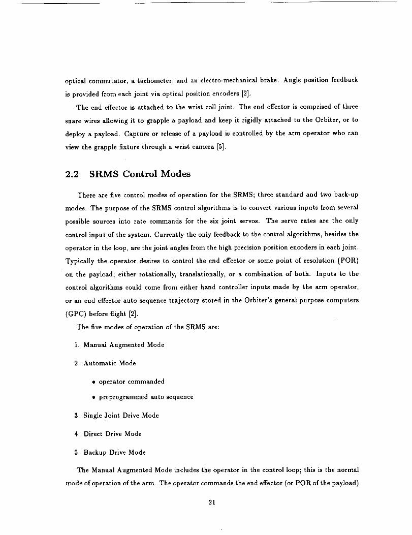
2.2 SRMS Control Modes

There are five control modes of operation for the SRMS; three standard and two back-up

modes. The purpose of the SRMS control algorithms is to convert various inputs from several

possible sources into rate commands for the six joint servos. The servo rates are the only

control input of the system. Currently the only feedback to the control algorithms, besides the

operator in the loop, are the joint angles from the high precision position encoders in each joint.

Typically the operator desires to control the end effector or some point of resolution (POR)

on the payload; either rotationally, translationally, or a combination of both. Inputs to the

control algorithms could come from either hand controller inputs made by the arm operator,

or an end effector auto sequence trajectory stored in the Orbiter's general purpose computers

(GPC) before flight [2].

The five modes of operation of the SRMS are:

1. Manual Augmented Mode

2. Automatic Mode

• operator commanded

• preprogrammed auto sequence

3. Single Joint Drive Mode

4. Direct Drive Mode

5. Backup Drive Mode

The Manual Augmented Mode includes the operator in the control loop; this is the normal

mode of operation of the arm. The operator commands the end effector (or POR of the payload)

21

translational and rotational velocity using the two, three-degree-of-freedom hand controllers.

Commands from the hand controllers are resolved into joint rate commands by the SRMS

computers. The operator has a choice of four different coordinate operating systems [2]. In this

mode of operation, all joints can be commanded simultaneously.

Two types of Automatic Modes are available in the SRMS. In the operator commanded

auto sequence, the arm is driven along a 'straight line' to coordinates input to the GPC by

the operator during flight. During a preprogrammed auto sequence, the operator can select

up to four of 20 preprogrammed trajectories to execute at one time. These preprogrammed

trajectories, which are verified before flight, are composed of up to 200 straight line elements

stored in the GPC. The operator can select any point along the straight line elements as a

pausing point for the arm until he or she requests it to complete the trajectory [3].

In the Single Joint Drive Mode the operator can control an individual joint with the full

support of the GPC. The operator selects the joint and provides a fixed drive signal. The GPC

then interprets the appropriate rate commands. The remaining joints are kept in a Position

Hold status as described in Section 2.3 [3].

Direct Drive Mode is the first contingency mode of the SItMS. As in the Single Joint Mode,

the operator may command only one joint at a time. In this mode, the remaining joints are

deactivated and held in position by their brakes. Commands to the working joint are hardwired

to the Motor Drive Amplifiers (MDA). Commands bypass the GPC, data buses, and the servo

control loop [2].

The Backup Drive Mode is an additional contingency mode provided to help insure the

SRMS is fail-safe. Similar to the Direct Drive Mode, only one joint may be controlled at a

time. It is used when no primary drive channels are available. It bypasses all primary channel

electronics, including the GPC, and uses a separate Backup Drive Amplifier (BDA) and backup

motor commutator driven by a separate power source [3].

2.3 Position Hold

After completion of an SRMS maneuver in one of the three normal modes of operation,

each control servo is given a zero rate command for a short period of time (determined by

the payload/arm configuration). After the zero rate command, each servo drops into Position

22

t_

_Dt--

03

if)y-rr"¢D

3-t-O

Ot3.

Time

Figure 2.3. Typical SRMS Maneuver Profile

Hold Mode. This zero rate command period is the window in which the controllers designed

by Gilbert, et al.[1] reside. It is designed to damp end effector velocities as quickly as possible.

A typical SRMS maneuver time profile is shown in Figure 2.3.

As the name implies, the purpose of the Position Hold Mode is too keep the arm in a fixed

position. This mode is employed after a maneuver to give the SRMS time to settle and maintain

a fixed position and attitude. At this point the operator either moves on to the next maneuver,

or has reached the desired final position. This is actually a subtle point; between maneuvers of a

given series of maneuvers the operator is not necessarily concerned with a particular end effector

position and attitude, rather he or she would like all oscillations to stop before moving on to

the next maneuver. However, after the final maneuver of a sequence the end effector position

and attitude is the principal concern, especially in operations such as SSF assembly. For this

reason, linear controller designs presented subsequently will regulate end effector position and

attitude rather than its velocity.

During Position Hold Mode, joint angle positions measured via the joint angle encoders

are fed back to the servo control loops. It is important to realize that the joint angles are

23

convertedintojoint rate commands via proportional feedback only. With only the joint angles

provided to the servo control loops, no information about flexibility in the manipulator booms

is available. Currently the operator must wait for the arm structure to damp excitations in the

booms resulting from residual energies after a maneuver. Furthermore, while the SRMS is in

Position Hold, current guidelines allow Shuttle attitude reaction control system (RCS) firings.

In such a situation, Position Hold should maintain the end efl'ector in its current position and

attitude relative to an Orbiter-fixed reference frame. However, Shuttle attitude jet firings excite

considerable flex in the booms of the SRMS. Furthermore, when heavy payloads (>10K lbs)

are deployed on the SRMS, this RCS induced flexure can result in closed-loop Shuttle flight

control system instabilities.

If it is desired to reduce the fraction of mission time squandered waiting for the SRMS to

settle and to reduce dynamic interaction with other control systems, the benefits of focusing

on improving Position Hold Mode are apparent. Position Hold Mode is universal to the three

regular control modes; therefore, improving its performance improves the SttMS for its full

range of normal operation.

24

Chapter 3

Modelling the SRMS

Modelling is a delicate task of representing the dynamics of the Orbiter/SRMS/Payload

system which are important for the envelope of design while ignoring dynamics which are out-

side the envelope. We are interested in improving SRMS performance while it is operating in its

Position Hold Mode. Position Hold Mode is a regulator; one that desires to subdue initial con-

ditions (residual energies from arm maneuvers), and reject disturbances (introduced by Shuttle

attitude jet firings). In this mode, the arm is essentially in a fixed position; therefore, chang-

ing mass and inertia matrices associated with changing arm geometries are not a significant

factor. However, the six electro-mechanical control servos at the joints do contain substantial

nonlinearities in their dynamics which cannot be ignored.

The approach taken to modelling the SRMS is to divide the system into two subsystems.

First, the dynamics of the Orbiter/SRMS/Payload (arm) subsystem are considered without the

dynamics of the servos. Second, the control servo dynamics are modelled. A block diagram

depicts the total system in Figure 3.1.

Inputs to the 'arm dynamics' subsystem include Shuttle attitude thruster firings, sensor

noise, as well as the torques on each joint generated by their corresponding control servo.

These inputs are combined to determine the end effector acceleration. This acceleration is then

integrated to obtain the outputs of this subsystem which are end effector position and attitude

as well as the six joint angles. The joint angles are fed back through a proportional feedback

gain matrix to the control servos. If we consider the joint angle and end effector perturbations

to be small, which is the case in Position Hold, this subsystem is essentially linear.

The control servo subsystem consists of six servos which have as inputs joint rate corn-

25

servo uncertainties

S'nuttleattitude

A GS thrusteru_ firings

___ _u endeffector

servo dynamics state vector

Jdyna=ics.I

joint angle feedback to servos

.L

7c

joint ratecomznands

K(s)

r

sensor

noise

Figure 3.1. Block Diagram of the Compensated System

mands from a designed controller as well as the joint angles determined by the arm dynamics.

This subsystem has as outputs the torques generated on each joint. There are several nonlin-

earities present in each servo, including: current and torque limiters, trim integrator limiter,

gearbox stiffness, digital and analog tachometers, as well as joint motor stiction/frictions. The

approach taken to linearize this nonlinear subsystem is to treat the nonlinearities as modelling

uncertainties on a linear plant.

Section 3.1 generates the equations of motion for the Orbiter/SRMS/Payload system. Equa-

tions are generated in an Orbiter-fixed reference frame. The equations of motion are derived for

a simplified one joint example and then extended to six joints. Assumptions used in modelling

are also outlined.

Section 3.2 begins with a nonlinear model of the joint servos and obtains a simplified linear

model. This linear model is then combined with the arm plant in order to generate a linearized

model of the complete SRMS. In order to linearize the control servos, certain nonlinearities

are ignored which have minimal contribution in Position Hold Mode. The remaining nonlin-

earities are linearized by selecting 'nominal' values, but their effects are modelled as parameter

26

uncertainties on the linear plant. The standard three block form of a transfer function used for

design and robust analysis is introduced as well. The limitations of the methods used in this

Section are also discussed.

The resulting 24 state linearized model is compared with a higher fidelity nonlinear simu-

lation in Section 3.3. This nonlinear simulation has been compared with actual flight data to

confirm its accuracy. Comparisons are made in the time domain in Position Hold Mode. The

effects of varying the parameter uncertainties of the linear plant in an effort to capture the

range of the nonlinear behavior are also investigated. Section 3.4 draws the conclusions of this

Chapter. The deficiencies of the major assumptions used in this Chapter are also re-explored.

3.1 Equations of Motion for the Orbiter/SRMS/Payload Sys-

tem

Much of the derivation of the equations of motion in this section is based on the SRMS

simulator LSAD 1. LSAD is a higher fidelity nonlinear simulation of the SRMS and flight control

system of the Space Shuttle. Details on LSAD and the basis of this section can be found in

References [7],[8],and [9].

In deriving the equations of motion, the mass of the connecting structure between the Or-

biter and payload can be ignored when a payload mass exceeds 5,000 lbs. Previous simulations

have found this assumption to be reasonable. LSAD as well is based on this assumption. Ref-

erence [7] has the detailed derivation of the rotational dynamics between two bodies connected

via a massless, flexible structure. Rather than derive the six joint case, Section 3.1.1 examines

the one joint case and Section 3.1.2 extends it to six joints based on the work in Reference [7].

3.1.1 Equations of Motion for the Single Joint Case

Figure 3.2 represents the case of a single joint in Position Hold. The SRMS has been recast

as a point mass, m, oscillating on the end of a massless flexible beam which is attached to a

single joint. A joint in Position Hold behaves as a spring with some damping. Table 3.1 defines

the essential variables.

II,SAD standR for lmm Singing And Dancing; a take off of Spar Aer_paxe's ASAD: All Singing And Dancing.

27

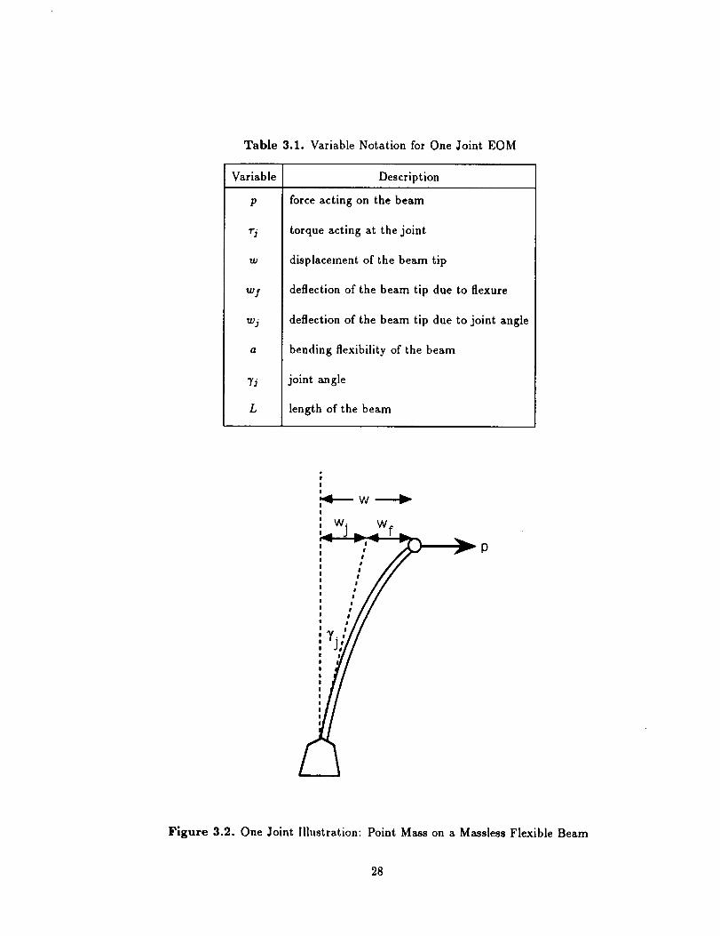
Table 3.1. Variable Notation for One Joint EOM

Variable Description

P

rj

IU

wl

wj

a

7j

L

force acting on the beam

torque acting at the joint

displacement of the beam tip

deflection of the beam tip due to flexure

deflection of the beam tip due to joint angle

bending flexibility of the beam

joint angle

length of the beam

P

Figure 3.2. One Joint Illustration: Point Mass on a Massless Flexible Beam

28

From these definitions

w = w I+w./ (3.1)

w./ = LT./ (3.2)

wf = ap (3.3)

Tj = Lp (3.4)

Therefore

w = L7. / + ap = LTj + a-_ (3.5)

From Newton's second law, in the absence of external forces, the force at the tip, or the

torque over the length, is equal to the acceleration of the mass

p -- _/'n_

When combined with Equation 3.4, this can be recast as

(3.6)

1

w = - m----_s2r./ (3.7)

Combining Equation 3.7 with 3.5 obtains

I[1]7./= -U _ + a _./ (3.s)

Equations 3.7 and 3.8 together achieve the objectives of determining the end effector posi-

tion, w, (position only for the one joint case) and the joint angle position, 7.i, given a torque

input to the system, rj. These two equations can be rewritten as

w = -s-2m -'L-'r./ (3.9)

7./ = -[ s-2L-'m-'L-' + L-'aL-'] rj (3.10)

Though this representation seems notationaily verbose, it will help motivate the sex joint

case. The extension of this problem to sex joints involves more complex notation, but essentially

the same concepts.

29

3.1.2 Equations of Motion for the Six Joint Case

In extending this problem to six joints and three dimensions, it is necessary to introduce

vector and matrix notation to keep track of positions and rotations. Furthermore, we will add

the effects of external forces caused by Shuttle attitude thruster firings to the system.

As before, E, will define the state of the end effector in an Orbiter-fixed reference frame.

Now, however, in three dimensions it is composed of a displacement vector and a rotation vector

w (3.11)

where _" is the vector defining the translational deflection of the end effector due to the applied

load. Similarly, _ is the vector defining the angular deflection of the end effector on each axis

due to the applied load. Since Position Hold Mode entails small variations about equilibrium,

rotations can be described by vectors. Table 3.2 makes similar definitions as before.

Table 3.2. Variable Notation for Six Joint EOM

Variable Description

7"

wf

wj

A

L

applied force from the payload at the end effector

applied moment from the payload at the end effector

vector of servo torques at each joint

end effector state vector

end effector deflection due to flexibility of the arm

end effector deflection due to rotations of the joints

6 by 6 flexibility matrix

joint angle vector

6 by 6 Jacobian matrix

As before, E may be decomposed as follows

w = wj + _f

30

(3.12)

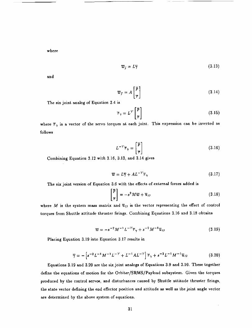
where

w%-= LV (3.13)

and

The six joint analog of Equation 3.4 is

where _7 is a vector of the servo torques at each joint.

follows

(3.14)

(3.15)

This expression can be inverted as

Combining Equation 3.12 with 3.16, 3.13, and 3.14 gives

-_ = L'_ + AL-'r_.r (3.17)

The six joint version of Equation 3.6 with the effects of external forces added is

[-ffT]=-s2M-_+_l) (3.18)

where M is the system mass matrix and _t_ is the vector representing the effect of control

torques from Shuttle attitude thruster firings. Combining Equations 3.16 and 3.18 obtains

-_ = -s-2 M -1L-'r_7 + s-2 M-l-at_ (3.19)

Placing Equation 3.19 into Equation 3.17 results in

"_= -[s-2L-'M-'L-'r+ L-'AL-'r]_7 + s-2L-'M-'-al, (3.20)

Equations 3.19 and 3.20 are the six joint analogs of Equations 3.9 and 3.10. These together

define the equations of motion for the Orbiter/SRMS/Payioad subsystem. Given the torques

produced by the control servos, and disturbances caused by Shuttle attitude thruster firings,

the state vector defining the end effector position and attitude as well as the joint angle vector

are determined by the above system of equations.

31

3.2 Modelling and Linearization of tile Control Servos

The general approach of this Section is to characterize the transfer function between the joint

angles, _', and the joint rate commands, _., to the torque output at the joints, _'r" Section 3.2.1

linearizes this nonlinear system, while Section 3.2.2 characterizes the effect of significant non-

linearities.

3.2.1 Control Servo Dynamics

The highest fidelity model of the SRMS servos available at Draper Laboratory is shown in

Figure 3.3. This model was designed to be accurate over a large frequency range and a wide

envelope of operations. This model is faithful enough to even encompass the accelerations of

the motor shaft while it transitions from forward driving to back driving 2 using simulation time

steps of 2 milliseconds [8]. References [8] and [10] show that for the low frequency oscillations

that occur with heavy payloads, much of Figure 3.3 can be eliminated•

References [8] and [10] both derive linearized models of the servo, but for slightly different

purposes. They do, however, provide useful insight into the nature of the nonlinearities as well

as the conditions in which they can be ignored. Figure 3.4 represents the linearized model of

the servos. Table 3.3 defines the variables of Figure 3.4. All quantities are either vectors or

matrices since there are six servos. The servos are all similar in configuration; differences occur

only in the values of the gear ratios, current limiters, moments of inertias, and gearbox stiffness.

Heavy payloads are assumed in modelling the arm dynamics. Draper's experience with the

SRMS in Position Hold mode demonstrates these conditions imply low frequency motions with

moderate amplitudes. This implies we can neglect high frequency dynamics. In linearization,

the effects of gear backlash, stietions, and frictions are ignored since they have negligible effect.

Simulations have shown that the integral trimmer has an effect only on motion when friction

is important; therefore, the trimmer and its limiter are eliminated from the linear model. The

analog tachometer with its high pass filter has negligible effects on low frequency motions, so it is

eliminated as well [8]. The digital tachometer's quantization effects are ignored; it is treated as

a linear gain. While in Position Hold, the current limiter saturates before the torque limiter so

the torque limiter can be eliminated from the model. Indeed, the most significant nonlinearities

2Forward drive occurs when the motor is driving the payload, lla_,k drive occur_ when the payload is driving the

motor.

32

!

I

u

I

--l-

I

i

i

I

Figure 3.3. Draper Servo Model

33

Table 3.3. Variable Notation for Servo Parameters

Variable Description Units

.2.."

7o

.2."

¢

N

K1

KI_A

KA

K't'/Rj.

KH

K,_ A

Kr_

K(;

Joint Angle Vector

Vector of Torque at each Joint

Joint Rate Commands

Motor Shaft Angle Vector

Motor Shaft Rate Vector

Gear Ratio

Motor Speed Command Scaling Gain

radians

ft-lb

rad/sec

radians

rad/sec

count/rad/sec

Digital-to-Analog Converter Gain

Motor Drive Amplifier Gain

Motor Torquing Gain

Effective Gain of Digital Tachometer Processing

Motor Back EMF Constant

Gain of the Forward Path: KI_AKAK't'/RI.

Gain of the Feedback Path: KI_ + K8/Kj_AKA

Motor Rotor and Gearbox Input Shaft Moment of Inertia

Gearbox Stiffness

v/cnt

v/v

ft-lb/v

cnt/rad/sec

v/rad/sec

ft-lb/cnt

cnt/rad/sec

slug-ft 2

ft-lb/rad

34

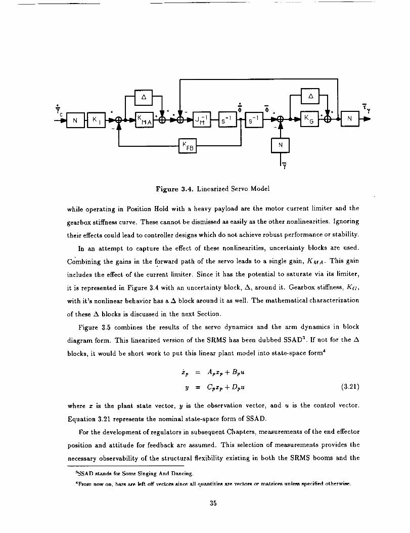
Figure 3.4. Linearized Servo Model

while operating in Position Hold with a heavy payload are the motor current limiter and the

gearbox stiffness curve. These cannot be dismissed as easily as the other nonlinearities. Ignoring

their effects could lead to controller designs which do not achieve robust performance or stability.

In an attempt to capture the effect of these nonlinearities, uncertainty blocks are used.

Combining the gains in the forward path of the servo leads to a single gain, K,_A. This gain

includes the effect of the current limiter. Since it has the potential to saturate via its limiter,

it is represented in Figure 3.4 with an uncertainty block, A, around it. Gearbox stiffness, K(;,

with it's nonlinear behavior has a A block around it as well. The mathematical characterization

of these A blocks is discussed in the next Section.

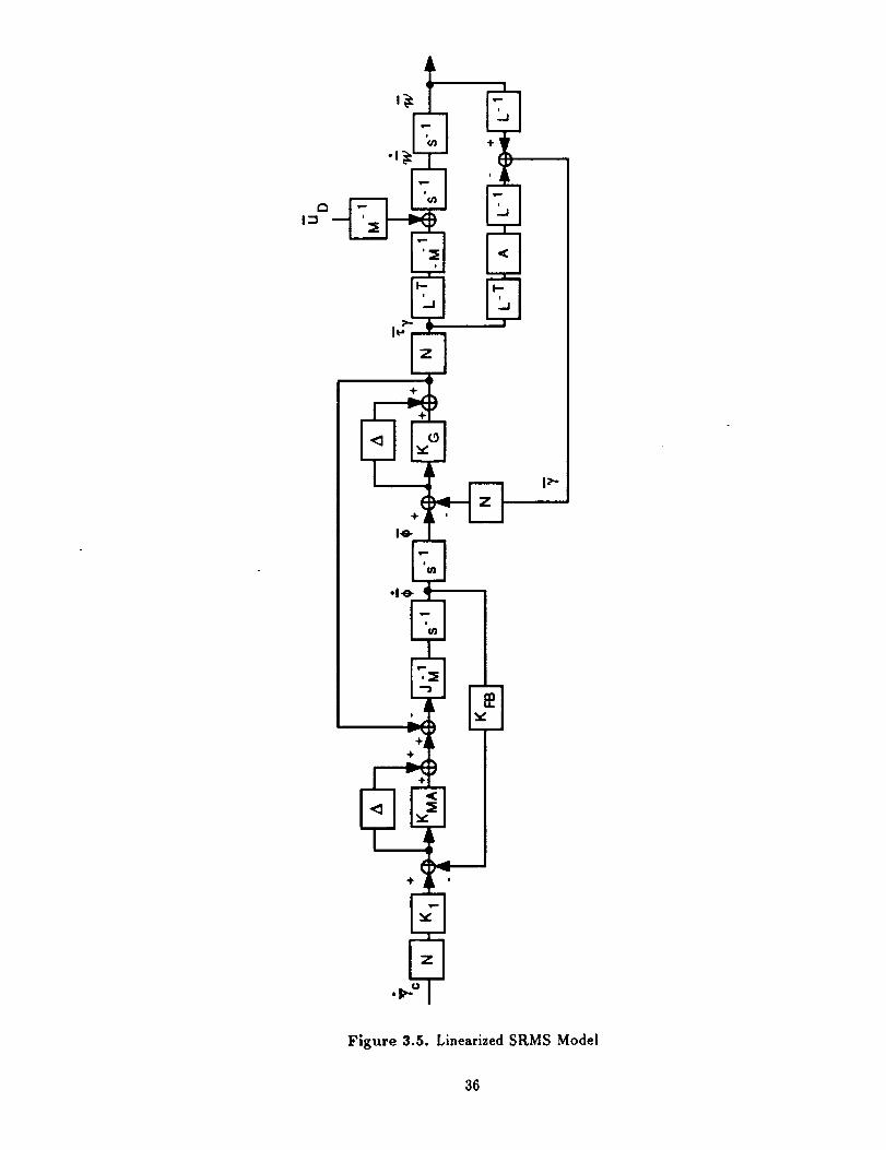
Figure 3.5 combines the results of the servo dynamics and the arm dynamics in block

diagram form. This linearized version of the SRMS has been dubbed SSAD "_. If not for the A

blocks, it would be short work to put this linear plant model into state-space form 4

(3.21)

where z is the plant state vector, y is the observation vector, and u is the control vector.

Equation 3.21 represents the nominal state-spaceform of SSAD.

For the development ofregulatorsinsubsequent Chapters, measurements ofthe end effector

position and attitude for feedback are assumed. This selectionof measurements provides the

necessary observabilityof the structuralflexibilityexisting in both the SRMS booms and the

aSSAD stands for Some Singing And Dancing.

4From now on, bars are left, off vectors since all quantities are vectors or matrices unles_ specified otherwi_.

35

i-_

J_

Figure 3.5. Linearized SRMS Model

36

gearboxes at each joint. There are several types of sensor suites that can recover this type of

information, including force-torque sensors, strain gauges, or accelerometers. Eventually, the

NASA/Johnson Space Center (JSC) plans to incorporate one of these set-ups into the SRMS

system.

3.2.2 Representing the Uncertainties

The method of characterizing parametric uncertainty presented in this Section follows the

work of Reference [11]. As shown in Figure 3.5, the state-space model of SSAD is a functiola

of several physical parameters, two of which, K(i and KM A, are uncertain. Using the form of

Equation 3.21 it is possible to model these parameter errors as

( ) ( k )_p = Ap+_AA_6i xp+ Bp+_AB_6_ uI=1 i_1

y = + ACi6i z_, + Op + ADi_i ui=1 i=I

where each 6i represents a parameter error that has been normalized as

-1 </i_< 1 Vi

As this suggests, the nominal value of both Ke; and K_,_A must be bounded equally from

both above and below. Consider K¢; first.

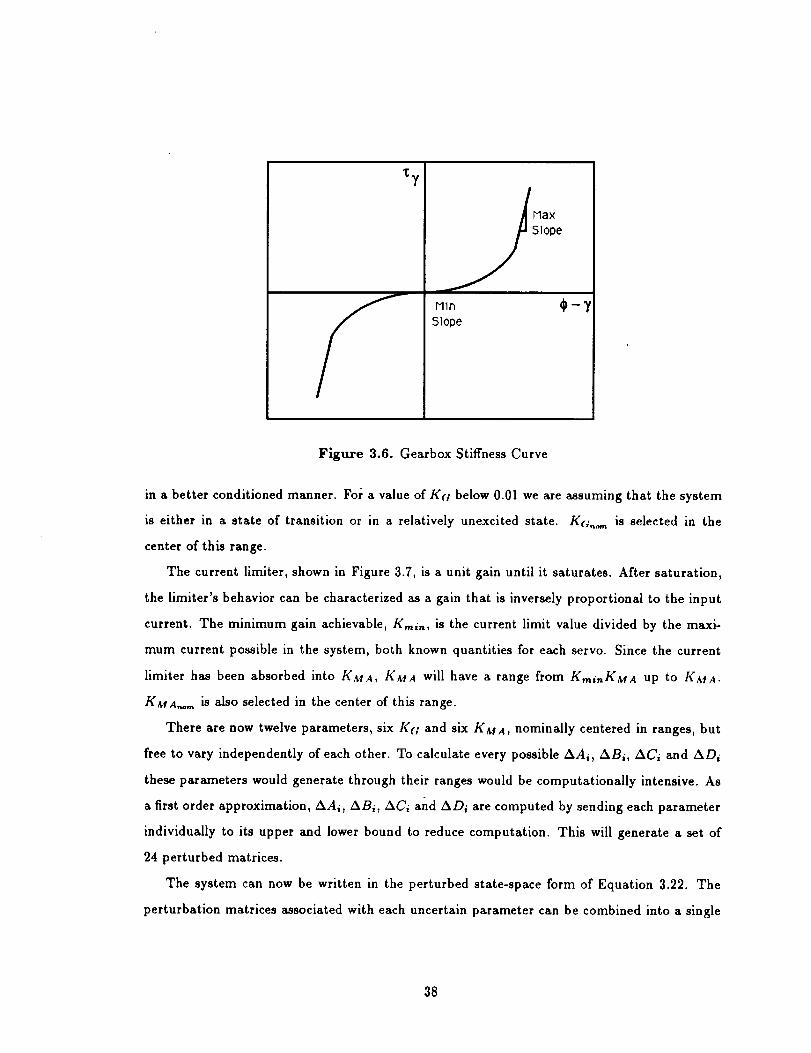
The gearbox stiffness curve is shown in Figure 3.6. The gain, Kt;, is the slope of the curve

at the point ¢ - 7. This slope can achieve values from zero up to a maximum slope that is

determined by the servo under consideration. One choice that captures all possible values of

Ke; is to choose the nominal value as half the maximum attainable slope with bounds above and

below of also half the maximum slope. This, however, will introduce problems when performing

robust analysis. Allowing a zero value for K(; is essentially allowing for the possibility of the

servos to be cut off from the rest of the system. All of the servos' associated dynamics would

become both uncontrollable and unobservable to any controller. Such a system will always fail

robust stability analysis. This, however, is a mathematical fiction. The system's manifestation

in a zero Kel state is transient, not a situation which the controller must deal with for any

length of time. A gain of 0.01 is used as the minimum value of Kei in order to pose the bounds

37

_7

Min $-751ope

Figure 3.6. Gearbox Stiffness Curve

in a better conditioned manner. For a value of Ktl below 0.01 we are assuming that the system

is either in a state of transition or in a relatively unexcited state. Kt;,,_ is selected in the

center of this range.

The current limiter, shown in Figure 3.7, is a unit gain until it saturates. After saturation,

the limiter's behavior can be characterized as a gain that is inversely proportional to the input

current. The minimum gain achievable, Kr_in, is the current limit value divided by the maxi-

mum current possible in the system, both known quantities for each servo. Since the current

limiter has been absorbed into KMA, K_¢A will have a range from K,,inKMA up to KMA.

K_r A._ is also selected in the center of this range.

There are now twelve parameters, six Kt; and six KMA, nominally centered in ranges, but

free to vary independently of each other. To calculate every possible AAi, ABi, ACi and ADi

these parameters would generate through their ranges would be computationally intensive. As

a first order approximation, AAi, ABi, ACi and ADi are computed by sending each parameter

individually to its upper and lower bound to reduce computation. This will generate a set of

24 perturbed matrices.

The system can now be written in the perturbed state-space form of Equation 3.22. The

perturbation matrices associated with each uncertain parameter can be combined into a single

38

_in

_0ut

Current Limit -

o o

oo •

• s S• _mln o

ir ._

Imax

Figure 3.7. Current Limiter

matrix

IAAiAB']7_ (n'+"_)×('_'+'_') (3.23)Ni : E

ACi ADi

where n_, = dim(z), n, = dim(y), and n,, = dim(u). This matrix is not full rank for the SSAD

system since any one parameter does not affect all of the states and outputs. Ni can therefore

be decomposed as

where for Rank(Ni) = hi, Qi E 7_ n'×r", Ri E 7_ '_x'_, Si E 7_ n_×'_', 7] E ./_,_i×,h, The

state-space model of the perturbed system can be rewritten as

kkp = Av + Z Qi6ilniSi

i--|

= A?z? + [Q1 ... Qk]

k= Cp + _ Ri6iI_Si

i----1

zp +

qk

zp +

. ]Bp + Z Qi6iI,..Tii=1

U

+ B_,u (3.25)

[ ' ]D? + _ Ri6ilmTii--1

u

39

i + Dpu

Tlk

(3.26)

[]is,]ii = ' zp + : u (3.27)

_k S_ Tk

The ei represent the inputs to the uncertainty block, A. They are a function of z/_ and u.

The _h represent the outputs of the uncertainty Mock which will influence the state dynamics.

This models the effect the parameter uncertainties have on the plant dynamics. Define

Q - [Q, .-. Qk]

/_ -= [R, ...Rk]

s ...

T =_ [Ti"...T'k"]

Augmenting the unperturbed state-space of Equation 3.21 with process noise, w, measure-

ment noise, u, and the effects of parameter uncertainty as defined above gives

:ip = Al, x n + Bnu + B,,,w + Q_?

y = Cnzp+Dpu+D_,v+Rr I

e = Sxp + Tu (3.28)

Figure 3.8 represents the general transfer function of a nominal plant, P(s), and compen-

sator, K(s), with parametric uncertainty, A. In this representation, d represents all exogenous

inputs into the system; in this case

[w]d - (3.29)//

and e is an error vector of signals of interest to be defined later. The state-space representation

of Figure 3.8 is

4O

d

---[A

T/

U

e

|

Figure 3.8. Standard Form for a Compensated Plant with Uncertainty

= Ax+BI,I+B2d+B3u

e = Clz+Dllrl+D12d+Dlzu

e = C2z + D21'1 + D22d+ D2.au

y = C._x + D._2rl + D32d+ D.a3u (3.30)

Placing Equation 3.28 in the form of Equation 3.30 gives

___] ApSi

y .C_

Q B_ Bp

0 0 T

D2, D22 D2.a

R D.a2 Dp

_p

d(3.31)

B_ = [B,,,i0(..x_v)]

D,_2 - [0(nyx_,,)iD_]

Equation 3.31 represents the state-space equation for the linearized SRMS with the nonlin-

earities KA_ A and Ke; modeled as parameter uncertainties. One clarification needs to be made

about the matrix B_. This matrix characterizes how the process noise affects the state. This

matrix comes from the ut) term of equation 3.19. ut) represents the effect of Shuttle attitude

thruster firings on the end effector. Recall that while in Position Hold mode the Shuttle is

41

restricted from using its translational thrusters, therefore ul_ will effect only the rotational

states. However, for computation of a linear optimal estimator such as one employed by model

based compensators, every state must be controllable by the noise. To avoid problems before

they occur, the effects of fictitious Shuttle translational thruster firings are added to//2.

The actual construction of uij depends upon the Orbiter/Payload configuration. On a given

Shuttle mission, pre-flight evaluations select a certain set of jets to fire for a roll, pitch or yaw

command for a given Orbiter/Payload configuration. Barring a system failure, those same jets

are used every time. Since the force a particular jet will impart to the end effector can be

calculated, the disturbance vector, ul_, has six elements corresponding to a roll, pitch, yaw,"

x translation, y translation, or z translation command. Such a command is normalized to lie

between -1 and 1 corresponding to, for example, a -roll command or a +roll command.

3.3 Comparison of the Linear and Nonlinear Plant

There are several simplifications made in developing the linearized SSAD from the nonlinear

LSAD. This Section compares the two simulations to expose the deficiencies in the linearization

process. Frequency domain information such as singular value decompositions are not available

for the LSAD. Instead, comparisons are made in the time domain while running both systems

in Position Hold Mode. Figure 3.9 shows a block diagram of SSAD in Position Hold Mode.

The Position Hold controller does nothing more than feed back the joint angles, 7, to the servos

through a set of gains, Ky.

The Hubbh Space Telescope (HST) in its release configuration is selected as the payload on

a standard Orbiter. HST weighs 25,000 Ibs, so the heavy payload assumption is not violated.

HST in its release configuration will be used in subsequent Chapters for all designs since when

this research began, ample data was available on this payload in this configuration.

Recall that both Kt,¢A and K(; have a range of values. The nominal state-space, Pno,,_(s),

places both K_A and K(_ at the midpoint of their respective ranges. Since Pno,,,(s) is the

plant that will be used in controller design, Photo(S) in Position Hold Mode is compared with

LSAD.

Both SSAD and LSAD are run in a Position Hold closed-loop with initial conditions on

end effector velocity, w. This scenario models the situation occuring when the SRMS drops

42

sefvo dynamics

Gs(S)

Yc

joint ratecommands

arm dynamics

(s)

m

Y

Position

Hold Gains

Figure 3.9. SSAD in Position Hold

into Position Hold Mode following a maneuver; the SRMS is instructed to maintain it's current

position and attitude though residual velocities remain from the maneuver. Recall that the end

effector state vector is constructed as follows

X position

Y position

[_] Z position= = (3.32)

Roll attitude

Pitch attitude

Yaw attitude

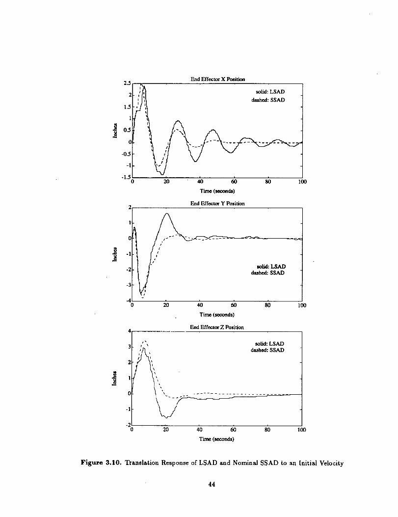
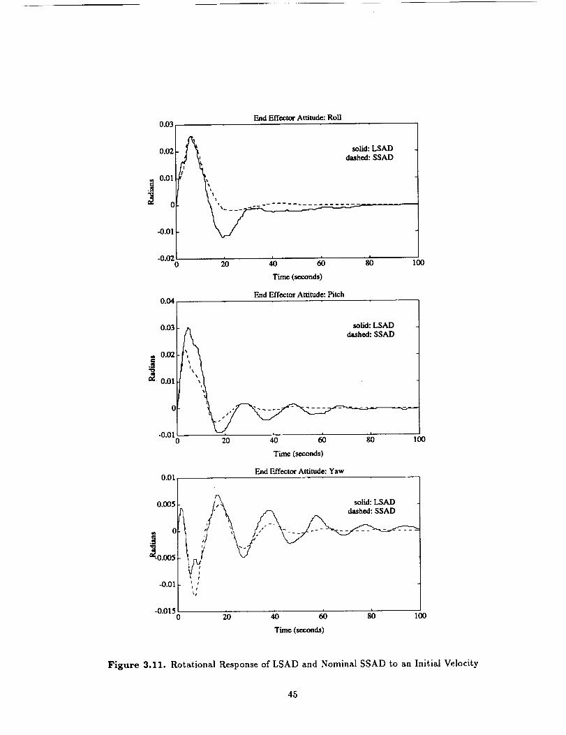
Figures 3.10 and 3.11 compare the translational and rotational response of the end effector

to an initial velocity for both LSAD and the nominal SSAD. Both amplitudes and frequencies

are similar. Considering the linearization process, SSAD compares reasonably well with LSAD.

Recall that Figures 3.10 and 3.11 represent the nominal SSAD plant. In the nominal plant,

both Kava and K(; have been placed in the center of their ranges for design and robust anal-

ysis purposes. Hopefully, the uncertainty ranges on these gains capture the behavior of the

nonlinear plant. Following this logic, there should exist off-nominal values for both KMA and

K(; that will make the comparison between LSAD and SSAD more favorable for these initial

conditions. Looking at Figures 3.10 and 3.11 it seems that SSAD is damping quicker than

43

¢.}

2.5

2

1.5

1

0.5

0

-0.5

-1

-1.50

2

1

0

-1

-2

-3

-40

4

3

2_I

C

-1

-20

End Eff_tor X Position

|1

II

• i

solid: LSAD

dashed: SSAD

20 40 (_) 8(} 100

Time (seconds)

End Effoctor Y Position

mlid: LSADdashed: SSAD

/,io 6b 8b

Time (seconds)

End Effoctor Z Position

100

r x solid: LSAD

/_._,'' dashed: SSAD

10 40 60 80 100

Time (seconds)

Figure 3.10. Translation Response of LSAD and Nominal SSAD to an Initial Velocity

44

0.03

0.02

= 0.01

o

-0.01

-0.020

0.04

End Effector Attitude: Roll

solid: LSAD

: _ dashed: SSAD

_o /o _ 8b

Time (seconds)

End Effector Attitude: Pitch

100

0.03

= 0.02.I2 0.01

-0.010

0.01

0.005

-0.01

solid: LSAD

dashed: SSAD

20 40 60 80 I00

Time (seconds)

End Effector Attitude: Yaw

solid: LSAD

/ \_/__ dashed: SSAD

-0"0150 :20 40 60 8() 100

Time (seconds)

Figure 3.11. Rotational Response of LSAD and Nominal SSAD to an Initial Velocity

45

LSAD. After moving K(; towards the lower end of its range to compensate this damping, and a

little experimentation with increasing KAVA as well, Figures 3.12 and 3.13 present an improved

match between LSAD and SSAD.

3.4 Conclusions

This Chapter uses several assumptions to bring the SRMS Position Hold plant into a

workable linear form. SSAD model accuracy is restricted to payloads greater than 5,000 lbs.

This is not a crippling assumption. The 25,000 lbs Hubble Space Telescope is used for design in

this thesis. Other assumptions are made in linearizing the nonlinear plant. Several nonlinearities

are ignored whose effects are small in the envelope of design. That is, they either have negligible

contribution, or dominate at high frequencies. Two significant nonlinearities, KMA and K(_,

are represented as parameter uncertainties. These steps are all necessary to obtain a workable

plant model such that linear control design techniques can be applied. The drawback, however,

is that even if robust stability can be guaranteed on SSAD, this guarantee will not translate

to the full nonlinear plant. SSAD can provide a reasonable indication, but not an assurance of

robust stability. The standard three block form for design and robust analysis presented in this

Chapter will be exploited in subsequent Chapters to provide easy ways to compare controllers

designed by different techniques.

46

_s

-1

-20

2]

1;

0

-1

-2

-3

-4

-50

End Effector X Position

t!

:A solid: LSAD

_t dashed: SSAD

I i

I f .#

11 iI J

I% If

io _o _ _ looTime (seconds)

End Effector Y Position

L

solid: LSADdashed: SSAD

Time (seconds)

End Eff_tor Z Position

100

2

1

0

-1

% io _o _ 8b

,. solid: LSADr

,_ L dashed: SSAD

'_ _ , ..... _ .......... _- ............

10o

Time (seconds)

Figure 3.12. Translation Response of LSAD and off-nominal SSAD to an Initial Velocity

47

0.03 End Effector Attitude: Roll

i

0.02

0.01

-0.01

-0.020

0.04

Time (seconds)

End Effector Attitude: Pitch

IO0

0.03

0.02

•_ 0.01

0

-0.01

.-_

tt

-0.02 o :_o _o _ 8b loo

0.01

Time (seconds)

End Effector Attitude: Yaw

0.005

-0.01

-0.0150

:"/._x_f_ _ solid: LSAD

,

1

, , , , 1

20 40 60 80 100

Time (seconds)

Figure 3.13. Rotational Response of LSAD and off-nominal SSAD to an Initial Velocity

48

Chapter 4

Design and Analysis Approach

The 24 state linearized model of the SRMS developed in Chapter 3 is used in subsequent

Chapters for regulator design using three techniques: LQR, H2, and Hoo optimization. Before

any of these techniques are pursued, it is appropriate to consider the characteristics of the

open-loop plant and their possible effects on the design process. This Chapter examines several

aspects of the plant and anticipates how some can cause problems in both the design and

analysis process 1. Stability and performance criteria upon which each regulator design are

evaluated is introduced as well.

Section 4.1 examines the open-loop plant and suggests advantages of precompensation loop

closure. Model reduction is applied to the open-loop plant to reduce it to 18 states, thereby

reducing the order of any resulting compensator. The singular values of the reduced order

system are compared to the full order system. The poles and transmission zeros of the reduced

order plant are evaluated. Issues such as controllability and observability are also considered.

Section 4.2 concentrates on analysis of the open-loop plant. The criteria considered are

the same that are applied to each compensator design in order to provide a common measure

for evaluation. The singular values of the transfer functions from disturbance to end effector

position and attitude are inspected. The transfer function from disturbance to control effort is

scrutinized as well. In face of the parametric uncertainty present in SSAD, robust stability is

considered via the small gain theorem. As a less conservative method, the structured singular

value, p, is also used in analysis. Due to the nature of the uncertainty, p-analysis is still

IThis may aee, m like forenight in the thesis, though it is ac.tually hindsight in the reae.arch.

49

conservative. The impact this will have on the analysis process is explored as well.

4.1 Obtaining a Design Plant

The first inclination when designing a new compensator for a system is to remove the

old compensator and then proceed to the design process with the resulting open-loop plant.

Such an open-loop plant was presented in Figure 3.5. The poles of this open-loop plant are

plotted in Figure 4.1. With no feedback to the system, as expected, there are six poles residing

at the origin. These rigid body modes, though not welcome, would be accepted except that

computationally they do not appear exactly at the origin. Machine precision places them at

some small _ on either side of the jap-axis. This _ propagates through the design process causing

computational problems later.

One method of dispensing with this dilemma is to leave the joint angle feedback loop intact.

The current Position Hold controller as shown in Figure 3.9 consists of only a gain matrix.

Leaving the current Position Hold loop in place and designing around it can be thought of as

precompensation loop closure. Since there are no dynamics associated with the Position Hold

gains, designing around them will not increase the order of a resulting compensator. There are

several advantages to this precompensation loop closure.

Each joint operating in the current Position Hold Mode behaves as a spring with damping;

the joint angle feedback of Position Hold will pull the origin poles decisively into the left

half plane. This not only alleviates the computational problems discussed above, but it also

produces a non-singular system A matrix. Invertability of the system would allow for the

application of loop-shaping techniques in the LQG/LTR methodology such as those presented

in References [13] and [12]. Furthermore, when designing an enhancement to a system already

in use, it is conceptually more palatable to design the upgrade as stability or performance

augmentation such that the improvement will work around the current system rather than

replacing it. If necessary, the augmentation to the software can be dissabled leaving the orginal

system intact.

For the reasons outlined above, the current Position Hold system is treated for all intents

and purposes as the open loop plant. Henceforth, in all discussion of analysis of the open-loop

plant, it is the original Position Hold system that is actually being considered. The poles of

50

0.06Distant Poles (6)

0.04 ..................... _..................... + ..................... _ ..................... ; ..................... <.....................

0.02 ..................................................................................................................................

0 ................ "_': ............................................ _¢"........................................... "_'"'_( ...............

-0.02 .................................................................................................................. _......................

-0.04 ........................................................................................................................................

-0.06-650 -640 -630

3

2

1

0

-1

-2

-3

-620

Real

Near Poles (18)

-610 -6O0

iX

-59O

-0.35 -0.3 -0.25 -0.2 -0.15 -0.1

Real

Close-up of Origin Poles (6)

-0.05

I

0.5

0

-0.5

-I

-1.5-5

x _x

X:

X:

-4 -3 -2 -1 0

Real

X

3 4

x10-14

Figure 4.1. Poles of Open-Loop SSAD

51

this system are shown in Figure 4.2.

The six distant poles, which correspond to the dynamics of the motor rates, are considerably

faster than the rest of the system. They are even faster than the fastest possible sample rate

of 80 milliseconds in the actual system. Eliminating the fast poles will reduce the model to

18 states and thereby reduce the order of a compensator. As long as the bandwidth of a

compensator designed from the reduced order model (ROM) is kept relatively small, there will

be no interference. To insure problems do not occur with performance or stability as a result

of the model reduction, the ROM is used for controller design purposes only. The full order

model (FOM) is always used in analysis. This will isolate stability robustness problems to the

parameter uncertainties rather than confusing the issue with neglected dynamics. Section 4.1.1

examines a method for eliminating the fast dynamics of the system, while Section 4.1.2 explores

the characteristics of the ROM and compares it to the FOM.

4.1.1

as

Model Reduction

Denote the transfer function from joint rate commands to end effector position and attitude

G(s) := (A, B, C, D)

This can be decomposed as

c(s) = [o(s)L + (4.1)

where

represents the slow modes of the system, and

Ec¢,)],:= B,. b,)represents the fast modes to be cut from the system. Finding the matrices which define the

decomposed system requires the use of the algorithm presented in Reference [14] in the manner

outlined below:

Using an ordered Schur decomposition, find a unitary matrix, V such that

A = VAV'r= .All .412 ](4.2)

0 ,422 J

52

0.06Distant Poles (6)

0.04

0.02

0

-0.02

-0.04

0%50 -640 -630 -620 -610 -600 -590

Real

Near Poles (18)

0

-1

-2

-30.8

X

X

X

X X

X X X

x x

X

x

X Xix

x X

-0.7 -0.6 -0.5 -0.4 -0.3 -0.2 -0.1 0

Real

Figure 4.2. Poles of the Position Hold Open-Loop SSAD

53

Consider ;li to be the i _h eigenvalue of some matrix, A. Using the ordered Schur form, one

can find All and A22 such that

For SSAD, the system is divided into its 6 fast modes and 18 slow modes. Next, solving the

following equation for X

and then computing

and

.'i.tl X - X,'i22 +fi-12 = 0

[°1'-xl= VB/}2 0 I

(4.4)

(4.5)

[C' C2] =cv'r I Io X ]I

one arrives at the state-spa_e forms

(4.6)

[A,_ /}1 1[G(s)]., := C, D

[G(s)]; := [ A''d_ /}2]0

(4.7)

(4.8)

Notice that the full DC term of the system, D, is preserved in the slow system. Removing

the 6 fast poles in this manner reduces the system to 18 states. The next Section will examine

what information is lost in the reduction process and explore what effect this will have on

design.

4.1.2 Characteristics of the ROM

Figure 4.3 plots the singular values of the ROM and the FOM. No information is lost until

well beyond the bandwidth of the open-loop system. In the lower frequency range where the

54

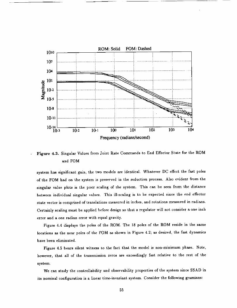
101oROM: Solid FOM: Dashed

107

104

o 101

10-2

10-5

10-s

10-11

10-14

: i.................................................. _........................ _.................................................. !..................................................

10-3 10-2 10-1 100 101 102 103 104

Frequency (radians/second)

Figure 4.3. Singular Values from Joint Rate Commands to End Effector State for the ROM

and FOM

system has significant gain, the two models are identical. Whatever DC effect the fast poles

of the FOM had on the system is preserved in the reduction process. Also evident from the

singular value plots is the poor scaling of the system. This can be seen from the distance

between individual singular values. This ill-scaling is to be expected since the end effector

state vector is comprised of translations measured in inches, and rotations measured in radians.

Certainly scaling must be applied before design so that a regulator will not consider a one inch

error and a one radian error with equal gravity.

Figure 4.4 displays the poles of the ROM. The 18 poles of the ROM reside in the same

locations as the near poles of the FOM as shown in Figure 4.2; as desired, the fast dynamics

have been eliminated.

Figure 4.5 bears silent witness to the fact that the model is non-minimum phase. Note,

however, that all of the transmission zeros are exceedingly fast relative to the rest of the

system.

We can study the controllability and observability properties of the system since SSAD in

its nominal configuration is a linear time-invariant system. Consider the following gramians:

55

3Poles (18)

X

x

x X

x X0 .................... )_ ...................................................................................... x ........... x .............. -x .......... _-x .................

X X

-I ..................................................................................................................................x........._....................................

X

X

-3 1-0.8 -0.7 -0.6 -0.5 -0.4 -0.3 -0.2 -0.1

Real

0

Figure 4.4. Poles of the Reduced Order Model

6OOTransmisson Zeros (12)

40O

200

0

-200

-4O0

"60_95

O

(D

®

O

O

300 305 310 315 320 325

Real

Figure 4.5. Transmission Zeros of the Reduced Order Model

56

A necessary and sufficient condition for controllability is that the controllability gramian

: ]' /4.9/

must be full rank. Dually, a necessary and sufficient condition for observability is that the

observability gramian

L,(,)--- fo' {eA'r'c"'CeA'} d_ (4.10)

must be full rank. If t is allowed to go to infinity and A is stable, then L_ and L, can be found

via the following Lyapunov equations:

ALe + L_A 't' + B B "1'= 0

A T L,, + L,_A + C'I'C = 0

(4.11)

Evaluating these gramians for the ROM ascertains the system to be fully controllable and

observable. Recall that the end effector position and attitude are the measurements used for

the new regulator designs. The controls are the six joint rate commands. Table 4.1 presents the

singular values for the controllability and observahi/ity gramians. Though the system is fully

controllable and observable to machine precision, this can be slightly misleading. Looking at

Table 4.1 some modes are clearly more controllable and/or more observable then others. This

implies that certain modes may require exorbitant amounts of control effort if they are to meet

certain performance requirements. Fortunately, however, all of the modes are stable.

All of these issues are important to keep in mind during the design process. There will be

limits to how far certain poorly controllable poles can be placed because of restrictions on the

control effort. Keep in mind that the reduced order model presented in this Section will only

be used for design purposes, the full order model will be used for analysis.

4.2 Analysis Techniques and the Open-Loop Plant

Before proceeding to design a new regulator to augment the performance of the current

Position Hold controller, let us consider Position Hold performance as it stands now. This

Section will analyze the current system following a threefold path. First, Section 4.2.1 considers

the transfer function from disturbance to end effector position and attitude respectively to

determine system performance. Second, Section 4.2.2 examines the transfer function from

57

Table 4.1. Gramian Singular Values

Controllability Gramian

Singular Values

2.0767e+07 2.1420e+05

2.0295e+07 1.3638e+05

7.1140e+06 8.5671e+04

1.8852e+06 6.6693e+04

1.8332e+06 4.7181e+04

1.4352e+06 2.6289e+04

9.2866e+05 2.7779e+00

3.5116e+05 1.1020e+O0

2.6732e+05 8.8740e-01

Observability Gramian

Singular Values

7.0207e+05 1.4658e-01

3.6847e+05 7.7801e-02

1.0944e+04 3.8524e-02

4.3336e+00 3.4467e-02

1.7348e+00 1.6510e-02

1.2482e+00 4.7992e-03

4.8469e-01 9.0874e-04

2.6327e-01 2.4196e-04

1.7180e-01 1.5619e-05

58

disturbance to control effort in order to establish how much control effort is required. Finally,

Section 4.2.3 looks at the stability robustness of the system. This method of system analysis is

the same procedure applied to every new controller designed in subsequent Chapters.

4.2.1 Performance

In evaluating the effect of a disturbance on the end effector state, only the rotational Shuttle

commands are considered since the effect of fictitious translational jets were added only so that

mathematically every state would have process noise. In fact, for Shuttle RMS operations,

translational commands are prohibited. As pointed out in Section 3.2.2, the disturbance is

normalized to lie between -1 and 1; let us consider the singular values from disturbance to the

end effector in two sets. The first set will include the end effector position in inches and the

second set will consist of the end effector attitude in radians. In this manner the singular values

will retain their units making the evaluation of performance an easier task. Figure 4.6 displays

these two sets of singular values for the current Position Hold regulator.

From Figure 4.6 we can see that the end effector excursion from equilibrium can be as great

as 5 inches in position and as much as 0.03 radians in attitude for certain Orbiter rotation

command directions. The goal in designing a new regulator is to bring these maximum excur-

sions down as hr as possible without exceeding the limitations on the control effort described

in the next Section. Ideally we aim for less than 1 inch excursion in position and less than 0.01

radians of rotation excursion.

4.2.2 Control Effort

There are already in place certain joint rate command limits, ie., limitations on the control

effort. These limits are not based on any hardware constraints, rather they are safety settings

to insure a payload at the end effector isn't commanded too rapidly bringing the system into

precarious areas of operation. These settings are a function of the payload inertia. The limits

are calculated to maintain a prescribed stopping distance when operating the RMS. If new

controllers can exhibit improved capability to control the end effector, there may be justification

for increasing the joint rate limits.

For design purposes, the joint rate limits will be treated as hard constraints that must

59

101

10o

104

._ 10-2

"_ 10-3

10-4

10-5

10-6

10-710-3

10-I

10-2

10-3

_ 10-4

10-5

10-6

10-7

10-8 '10-3

Singular Values from Disturbance to End Effector Position, , , ,,,,, .......... , , ,,,,, .... ,,,,,

..... i0-2 ..... i()-I .... i_ ..... ]'8'1 ..... 1'02

Frequency (radians/second)

Singular Values from DisturbancetoEnd EffectorAttitude• • .............. , ................... ,,,,

max: 0.0307

10-2 10-1 10o 101 102

Frequency (radians/second)

Figure 4.6. Performance Singular Values of the Current Position Hold System

60

Table 4.2. Joint Rate Limits

Joint Joint Rate Limit (rad/sec)

Shoulder Yaw

Shoulder Pitch

Elbow Pitch

Wrist Pitch

Wrist Yaw

Wrist Roll

0.0052

0.0052

0.0072

0.0107

0.0107

0.0107

be met. In this manner, the lower bound on performance will be established. Increasing the

joint rate limits will allow a new controller to use more control and thus allow performance to

improve. Table 4.2 presents the current joint rate limits.

To determine the control effort used by the system for a disturbance caused by Shuttle

attitude thruster firings, consider the singular values of the transfer function from the attitude

firings to each individual joint rate command. There are six joints and six different joint rate

limits. Let us scale each joint rate command by its corresponding joint rate limit. In this

fashion, as long as the singular values of these six transfer functions remain below unity, the

joint rate limits have not been exceeded. As Figure 4.7 shows, the current system is safely

below the joint rate limits.

Keep in mind that all performance and control effort analysis performed so far has been

on the nominal plant. Recall there are two parameters, KMA and Kt;, that include additive

uncertainty. The next issue to consider is robust stability in face of this uncertainty.

4.2.3 Stability Robustness

Recall the standard form for a compensated plant with uncertainty shown in Figure 3.8. The

closed-loop version of this is shown in Figure 4.8. G(s) is the closed-loop transfer function which

combines the dynamics of the plant and the compensator and A is the modeling uncertainty.

The closed-loop transfer function, G(s), can be divided into a set of four transfer functions

as follows,

61

10oSingular Values from Disturbance to Control Effort

. , , , , ,,,, , , , ......... ,,,,

10-1

10-2

"_ 10-3

10-4

10-5

101610-3 ..... i_ ...... i6_ ...... i_ .... io_Frequency (radians/second)

Figure 4.7. Control Effort Singular Values of the Current Position Hold System

eIt

Figure 4.8. Closed-Loop Transfer Function

62

Figure 4.9. Closed-Loop System for Robust Stability Analysis

[] Tclscsl[]e G_,(s)G22(,) d(4.13)

In this representation, the nominal closed-loop system is given by G22(s). Let us redraw

Figure 4.8 as shown in Figure 4.9. In this representation, looking at the A and Gll(s) transfer

functions, the small gain theorem can be invoked.

By invoking the small gain theorem, a sufficient condition for closed-loop stability is

IIG,,(s)AIIo_ < 1 (4.14)

The Ha norm is defined in the frequency domain for a stable transfer function matrix as

IIG(s)lloo = sup 5"[G(jw)]taJ

Ilyll_= sup

,..,_,,ollull_(4.15)

Therefore, the Ho_ norm is the induced 2-norm.

In Section 3.2.2, A was defined to be normalized to less than one. Therefore, Equation 4.14

can be reduced to

IlG_(s)ll_ < 1 (4.16)

This small gain test is valid for any complex A with norm less than one. However, for indepen-

63

dent modeling uncertainties, A is known to have a block diagonal structure

A

A, 0 ... 0

0 A2

: "'. 0

0 ... 0 A,,,

For the SSAD plant, there are two block diagonal elements for KMA and Kci. Since the small

gain test must hold for all normalized A, not just the more restricted set of normalized block

diagonal A matrices, An, it is a conservative test. Because it is known the perturbations of

SSAD are real parameter variations, testing for complex perturbations makes the small gain

test even more conservative.

In an effort to supply a less conservative robust stability test, Doyle [15] developed the

structured singular value,/_. /J is defined as

f

p[G(jca)] -- _ 0 if det[I - G(jw)A(jw)] # 0 for all A E A,_

[ {min,.xe,.xr_ _[A(jw)]} -1 det[l - G(jw)A(jw)] = 0 otherwise

(4.17)

Consider p[G,,(fla)]. From the definition of p, if p[G,,(jw)] > 1 at some frequency _a then

there exists a block diagonal A(jw) such that

&[A/(jw)] < 1 and det[I - G,l(jw)A(jw)] = 0

Conversely, if _[G,, (jw)] < 1 for all w, then the smallest block diagonal A matrix that makes

the system singular has the gain

> 1

which violates the norm of the modeling error. Therefore, a necessary and sufficient condition

for robust stability when A E An is

/_[G,,(jw)] < 1 Vw (4.18)

Unfortunately, in the actual application of/_-analysis we are reduced to conditions which

are sufficient but not necessary for two reasons. First of all, g is not a norm and it cannot be

computed easily. Software is available that can calculate upper bounds for/J. However, using

64

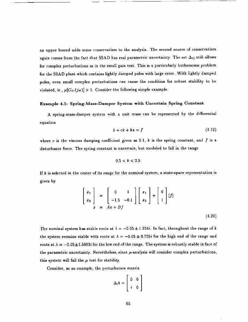
an upper bound adds some conservatism to the analysis. The second source of conservatism

again comes from the fact that SSAD has real parametric uncertainty. The set Aa_ still allows

for complex perturbations as in the small gain test. This is a particularly bothersome problem

for the SSAD plant which contains lightly damped poles with large error. With lightly damped

poles, even small complex perturbations can cause the condition for robust stability to be

violated, ie., p[Gll(jw)] > 1. Consider the following simple example.

Example 4.1: Sprlng-MassoDamper System with Uncertain Spring Constant

A spring-mass-damper system with a unit mass can be represented by the differential

equation

+ cz + kx = f (4.19)

where c is the viscous damping coefficient given as 0.1, k is the spring constant, and f is a

disturbance force. The spring constant is uncertain, but modeled to fall in the range

0.5 < k < 2.5

If k is selected in the center of its range for the nominal system, a state-space representation is

given by

z2 -1.5 -0.1 z2 1

= Ax+Bf

[f]

(4.20)

The nominal system has stable roots at )_ = -0.05 4- 1.224i. In fact, throughout the range of k

the system remains stable with roots at ,_ = -0.05 4- 0.705i for the high end of the range and

roots at _ = -0.054-1.5803i for the low end of the range. The system is robustly stable in face of

the parametric uncertainty. Nevertheless, since p-analysis will consider complex perturbations,

this system will fail the p test for stability.

Consider, as an example, the perturbation matrix

65

101 Small Gain Test (solid) Mu-Analysis(dashed), . ...... • • ............. N , . , , ,,,,,

10o

10-1

\ -

..... '1'0-2 ..... '1'0-1 ..... '1'_, l ....... i i i i ,i,,

101 102

Frequency (radians/second)

Figure 4.10. Robust Stability Analysis of the Current Position Hold System

whose norm is one. Though this perturbation cannot occur in the real system, p-analysis

will test for such a A. This perturbation places the roots at ,_1 = 0.3394 + 1.284i and A2 =

-0.4394 - 1.284i failing robust stability.

Though p-analysis does not supply a necessary condition for robust stability, it does reduce

conservatism over the small gain test. To illustrate this, Figure 4.10 displays the results of

the small gain test and p-analysis performed on the current Position Hold controller. Though

p-analysis is less conservative than the small gain test, the plant still fails robust stability.

To determine if the instability displayed in Figure 4.10 is the result of a fictitious complex

perturbation, or a configuration the system can actually realize, it is possible to evaluate the pole

locations of the system for different parameter values. To analyze every possible combination of

the twelve parameters would not be feasible; however, it is reasonable to check the endpoints.

Consider when the end effector is very close to its equilibrium position and attitude. At

these very small amplitudes, the current limiter has not saturated, hence all six of the KM A are

at their maximum values. Furthermore, at very small amplitudes the joint angles and motor

shaft angles are almost aligned, thus the six Kcl are at their minimum values. Figure 4.11

displays the pole locations of the system with the parameters Kt_ A and Kcl at these endpoints

66

0.5

0

-0.5

-1-0.2

Near Poles (18) Kg = 0.01x

X

X :X

X X

.... x-- • _.x- ............... X- .... x ........ •............... ..............................

XX

X

X...............................................................................................

X

X

-0.15 -0.1 -0.05 0 0.05 0.1

Real

Figure 4.11. Open-Loop System Near Pole Locations With K¢; = 0.01 and KAVA = KMA_.=

of their ranges.

As Figure 4.11 shows, the instability indicated by p-analysis is not fictitious. The system

isnot robustly stablefor the fullrange of values the parameters can inhabit. Ifallsix K(; are

increased in unison at 0.01 increments, the lowest values that achieve stabilityare 0.05. This

value brings the system poles just to the leftof the joJ-axis.This configuration isshown in

Figure 4.12. Interpretingthese observationsindicatesthe SSAD plant isa system that isstable

at moderate to high torque values when l((;ishigher than 0.05 and unstable at very low torque

values when K(; isbelow 0.05. Such a system would stably damp and then limit-cyclecloseto

the equilibrium position;such behavior isobserved in the actual system.

To totallyeliminate thislimitcycle behavior with a regulator may require a large sacrifice

of performance. In any case, itwould be misleading to think that eliminating such behavior

with a regulatoron our model would do so for the actual system. Recall that in Chapter 3 fric-

tionaleffectswere neglected in SSAD. Such effectswould certainlycontribute to the limitcycle

behavior. This issomething to keep in mind when designing new compensators. Instabilities

caused by very low K(; may not be a problem since they indicate slow limit-cyclingof small

67

2 Near Poles (18) Kg = 0.05

1.5

1

_, 0.5

-0.5

-1

-1.5

: 25

. x

.... X

X

x ×

X x

X

X

X

-0.2 -0.15 -0.1 -0.05 0

Real

Figure 4.12. Open-Loop System Near Pole Locations With Ktl = 0.05 and KMA = KMA,,,,,.,,

amplitude near the equilibrium values which is unavoidable.

4.3 Summary

In this Chapter, the 24 state SSAD model has been reduced to 18 states for design purposes

only. The 24 state model will be used for analysis purposes. Three criteria that will be

considered for each design are the performance singular values, the control effort singular values,

and robust stability of the plant. The analysis process was carried out on the current Position

Hold controller as both an example of the process and the baseline for comparison. In analyzing

performance, two sets of singular values were examined: disturbance to end effector position as

well as end effector attitude. Control effort was determined by looking at the singular values of

the transfer function from disturbance to control effort. Finally, robust stability was determined

via the small gain test, and the less conservative structured singular value,/J. /_-analysis may

still be too conservative a test since the SSAD plant is restricted to real parametric variations.

To determine this, we resorted to eigenvalue evaluation at certain parameter values.

68

Chapter 5

LQR Design

Linear Quadratic Regulator (LQR) design is very limited in its applications. This technique

not only requires knowledge of every state, but also, this knowledge must be uncorrupted by any

sensor noise. Since measurements of every state are not available, a linear quadratic regulator

cannot be implemented on the actual SRMS without first designing an estimator to approximate

the states. Nevertheless, it is useful to design a LQR because it gives an idea of the best we

can hope to achieve in terms of minimizing the '2-norm' of the error, Ilel12. It is a simple

first step that helps to motivate the model-based compensator (MBC) designs. In MBC design

techniques, the states of the system are estimated from the measurements. These estimates are

then used by a compensator. MBC design techniques are the topics of subsequent Chapters.

The LQR technique is derived from optimal control theory. Kwakernaak and Sivan [16]

provide the full details of this theory. Section 5.1 provides the main results of the LQR technique

as it applies to the SRMS problem.

Section 5.2 analyzes the LQR for the SRMS using the techniques presented in Chapter 4.

The performance and control effort singular values are examined and compared to the open-

loop system. A time domain simulation of a typical jet firing pattern is also presented. Finally,

stability robustness is examined in face of the parametric uncertainty.

5.1 LQR Theory

LQR theory provides no direct method to design for stability robustness or robust perfor-

mance, thus for design purposes Figure 5.1 eliminates the A block of Figure 3.8. The effects of

69

e

!

Figure 5.1. Plant With Compensator

the A block are considered after the design process is completed.

The general state-space representation of Figure 5.1 is

= C1 Dll D12

C2 D21 D22

(5.x)

In the LQR design methodology, uncorrupted full state feedback is called for. Thus the

disturbance vector, d, does not include sensor noise, only the process noise. Furthermore, C2

is the identity matrix. We will design the LQR compensator from the reduced order model

presented in the last Chapter. For analysis, we will apply the reduced order compensator

design on the full order plant. The result of an LQR design is well known to be a constant gain

matrix, thus an LQR does not increase the order of the closed-loop system.

The error vector, e, includes the states and the controls.

The states are weighted by a symmetric and positive semidefinite matrix, Q, while the controls

are weighted by a symmetric and positive definite matrix, R. Additionally, the modelling

performed in Chapter 3 produced no direct feedthrough term, thus D22 = 0. Hence for the

LQR formulation of the SRMS, Equation 5.1 can be recast as

7O

(5.2)

The LQR problem is to devise a feedback control law which minimizes the quadratic cost

functional

The optimal feedback controllaw is

(5.4)

where K is the symmetric, positive semidefinite solution of the algebraic Riccati equation

Ap'rK + KA 1, - KBpR -1B/rK + Q = 0 (5.5)

In general, there are many solutions to Equation 5.5, but only one of them is positive

semidefinite. The gain matrix K will exist and be positive definite provided that the system

(Ap, Bp, Q½) is stabilizable and detectable. In other words, any uncontrollable or unobservable

modes are asymptotically stable.

The closed-loop system dynamics become

£p = Apxp + Bpu + Bid

u = -Gxp

i_, = [Ap - BpG] xp + B1 d (5.6)

Furthermore, the closed-loop system is guaranteed to be stable, ie.,

ReAl [Ap - BpG] < 0 Vi (5.7)

The exact pole locations will depend not only upon the open-loop system (through Ap and Bp),

but also upon how the weighting matrices Q and R are selected. Thus Q and R are the design

parameters that are tuned until a LQR design meets desired disturbance rejection and control

effort requirements.

71

5.2 LQR Results

For the SRMS problem, the only states of concern are the ones corresponding to the end

effector position and attitude. To express this desire, Q is selected as a matrix of zeros except for

the values along the diagonal elements corresponding to the end effector position and attitude

states.

Recall that the end effector position is measured in inches and the attitude is measured in

radians. To scale the outputs, consider the singular values of the open-loop system as shown in

Figure 4.6. The attitude maximum singular value is more than an order of magnitude below the

position maximum singular value. The weights in Q are chosen to reflect this difference. The

elements of Q corresponding to attitude are placed more than an order of magnitude above the

position weights. In this manner a one inch error is not considered as serious as a one radian

error. The actual values of the weights do not matter, only the ratio between them. Such a

selection of Q also insures that the system (At, , Bp, Q½) is stabilizable and detectable.

In selecting R, certainly every control must be weighted to insure the joint rate limits are

not violated. As shown in Table 4.2, we already know the limit of control demand considered

acceptable. As a starting point, choose the inverse of the joint rate limits as the initial weight

and then iterate over the design process, tuning R each time until the singular values from

disturbance to control effort fall just below the joint rate limits for each control channel. This

procedure will result in the best performance possible with the LQR design technique given the

limits on the control effort.

Section 5.2.1 examines the control effort and performance singular values in the same manner

as outlined last Chapter. A time domain simulation is included as well to help interpret the

singular values. Section 5.2.2 examines the stability robustness of the LQR design.

5.2.1 LQR Control Effort and Performance

Figure 5.2 shows the singular values from disturbance to control effort after the iteration

process. Each control weight is fine tuned until the scaled singular value falls just below

one. Below 0.1 radians/second, the control effort has not changed much from the open-loop

system. For disturbances occuring at 1 radian/second, the LQR system uses almost two orders

of magnitude more control than the open-loop system. Nevertheless, the LQR system does not

72

100

10-I

1ff2

lff3I

lff3i i i I i It 'l , * , i t itl, , • , , * lift

1_2 1_1 1_

Singular Values from Disturbance to LQR Control Effort

\

\

...... ..... i!

Frequency (Radians/Second)

Figure 5.2. Control Effort Singular Values of the LQR System

exceed the joint rate limits.

Figure 5.3 presents the singular values from disturbance to end effector position and attitude.

Included on the same plots is the corresponding information for the open-loop system. For the

LQR design we were able to meet the performance goal of less than 1 inch excursion in position.

This is expressed by the maximum singular value falling below one for all frequencies. Thus

for any input disturbance, its effect on the end effeetor position will be multiplied by a gain at

least less than one. Since the input disturbance is already normalized to fall between -1 and

1, the maximum excursion of the end effector position is less than one inch. Similarly, since

the maximum singular value for the disturbance to attitude transfer function falls below 10-2

we have guaranteed less than 0.01 radians of rotation excursion. Both goals are met without

exceeding the joint rate limits.

To better visualize what is occuring on the singular value plots, a time domain simulation

is presented in Figures 5.4 and 5.5. These figures include both the response of the open-loop

system and the LQR system. In this simulation a roll command is given for a full 10 seconds

immediately followed by a 10 second pitch command and finally a 10 second yaw command.

From Figure 5.4 we can see that the X direction has considerably poorer disturbance re-

73

101

_ 100

_ 10-1

•_ 10-2

10-3

_, 10-4

,,_ 10-5

_ 10-6

10-7 '10-3

Singular Values from Disturbance to End Effector Position

................. "_""'_..................... t

-_'1-- _ x" "_.__

I i I • I .... i i I i i ii • • I , . l i i i i i , ii ..... i i i

10-2 10-1 i'_ 101 102

Frequency (radians/second)

10-1

10-2

C_ 10-3

._ 10-4

10-5

106

10-7

1_1_)-3 ..... 'l'&2

SingularValues from DisturbancetoEnd EffectorAttitude

N

',_","L\

,, N\

..... i'd_x..... i& ..... idl ..... i'd_Frequency (radians/second)

Figure 5.3. Performance Singular Values of the LQR System

?4

End EffectorX Position0.5. .,

V: """!

-1 It

t-1.5 i

I

iI-2

I-2.5

% _oTime (seconds)

8_

2.5End Effector Y Position

2.Q

0,-4

C

-0.5

_|

-1.5

/'1

sf %I

I

f

ii k

J I

I

,,-J

! ,

i1 I

_o /o _ 8bTime (seconds)

End EffectorZ Position

0.5

,_ o

-0.5

_ -1

_ -1.5-2

_ -2.5

-30

'1

\

'1

1

1

iI

f

If

¢

if

L fl

x )

100

100

_o _o _ _ _0oTime (seconds)

Figure 5.4. Translational Response of PH System and LQR System to Attitude Thruster

Commands

75

0.01End Effcctor Attitude:Roll

A

O.OO5

.005

_ o0.01

-0.020

k

1I

X

I L

I

1

I

I

If

't J

_o _ _ 8bTime (seoonds)

tO0

$3,x 10-3 End F_ector Attitude: Pitch

Ir I*1

k

-I0 _,

i -15

-20 o _0Time (seconds)

s6 100

0.02End Effector Attitude: Yaw

$0.015

0.01

._. 0.005

C

-0.005

/ ,: L

t

r x

o _o _o _ s6 iooTime (seconds)

Figure 5.5. Rotstionsl Response of PH System and LQR System to Attitude Thruster Com-

mands

76

°_,_

101

10o

10-1

LQR: Small Gain Test (solid) Mu-Analysis(dashed)

10-2 , , .....................10-3 10-2 '1'(_1 10o

-- X

\\

\ x

\

i

Frequency (radians/second)

Figure 5.6. Robust Stability Analysis of the LQR System

jection than the Y and Z directions. Nevertheless, significant improvement over the uncom-

pensated system is also apparent. Similarly, roll disturbance rejection is considerably better

than the other axes as shown in Figure 5.5. These plots indicate that while in ItST release

configuration, the SRMS can reject disturbances much easier in some directions over others.

5.2.2 LQR Stability Robustness

Applying both the small gain test and p-analysis to the closed-loop LQR system results in

Figure 5.6. Unfortunately the system fails both tests. Recall as outlined last Chapter that both

tests are conservative for SSAD since the uncertainties are real parameter variations. Therefore

it is possible that the system is in fact robustly stable in face of the uncertainty though it

cannot be shown.

Last Chapter, to confirm the results of p-analysis, we evaluated the eigenvalues of the

open-loop system for different parameter values. This technique conclusively showed that the

open-loop system was in fact not robustly stable. As before, we can evaluate the eigenvalues of

some combinations of the parameters to further our information on robust stability.

77

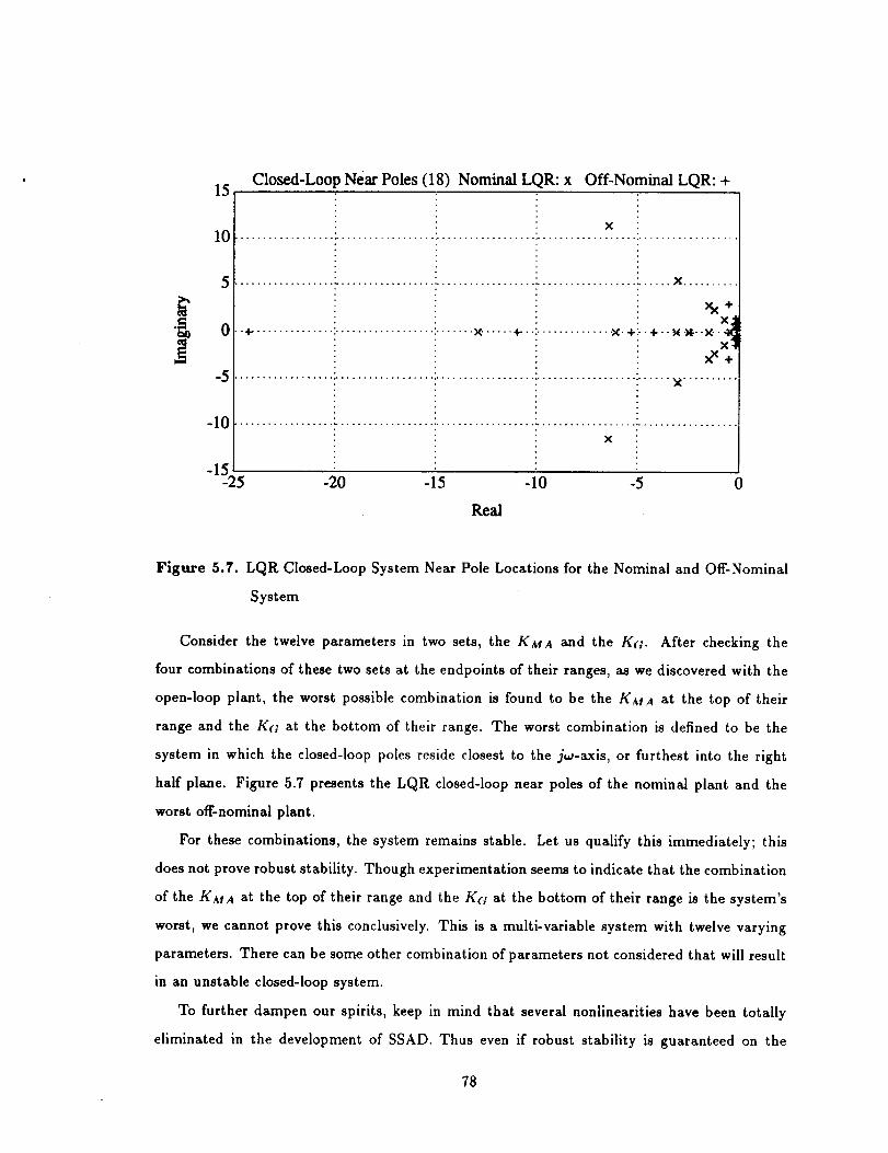
15 Closed-Loop Near Poles (18) Nominal LQR: x Off-Nominal LQR: +

10

0

-5

-10

-15

×

.............................................................................. X .........

XX+

X,"X" ..... 4- ............... "X'+:- +--N-_--X--_

X

xX+

................. ................... , .................. ° .................. ....... "_ .........

X

-25 -20 -15 -10 -5 0

Real

Figure 5.7. LQR Closed-Loop System Near Pole Locations for the Nominal and Off-Nominal

System

Consider the twelve parameters in two sets, the KMA and the Kt;. After checking the

four combinations of these two sets at the endpoints of their ranges, as we discovered with the

open-loop plant, the worst possible combination is found to be the Kt,_A at the top of their

range and the Kcl at the bottom of their range. The worst combination is defined to be the

system in which the closed-loop poles reside closest to the ja_-axis, or furthest into the right

half plane. Figure 5.7 presents the LQR closed-loop near poles of the nominal plant and the

worst off-nominal plant.

For these combinations, the system remains stable. Let us qualify this immediately; this

does not prove robust stability. Though experimentation seems to indicate that the combination

of the K/_A at the top of their range and the K(; at the bottom of their range is the system's

worst, we cannot prove this conclusively. This is a multi-variable system with twelve varying

parameters. There can be some other combination of parameters not considered that will result

in an unstable closed-loop system.

To further dampen our spirits, keep in mind that several nonlinearities have been totally

eliminated in the development of SSAD. Thus even if robust stability is guaranteed on the

78

model, it is not guaranteed on the actual system. We will not bypass the extensive pre-flight

simulation requirement of a Shuttle mission.

5.3 Summary

Using the LQR technique, we have designed a compensator that is capable of meeting the

performance objectives within the allowable control effort. The resulting regulator fails robust

stability analysis via both the small gain test and /_-analysis. However, actual eigenvalue

evaluation with four combinations of the parameters at their endpoints seems to indicate that

the system may be robustly stable. Unfortunately, this cannot be proven unequivocally.

There are several drawbacks to the LQR, technique. This technique not only requires knowl-

edge of every state, but also, this knowledge must be uncorrupted by sensor noise. These

requirements render an LQR design impractical for implementation of the actual SRMS. An

estimator would be required to determine the states for the LQR. This would add noise to the

state feedback vector which the LQR does not account for. If an estimator must be designed,

it is better to use an optimal design method such as the LQG technique.

79

Chapter 6

H 2 Design

Last Chapter we saw that with full state feedback, performance goals were met without

exceeding the control effort limitations. However, in the actual system we are limited to an

observation vector, y, which is some linear combination of the states corrupted by noise. The

solution to this more involved problem is given by the Linear Quadratic Gaussian (LQG) theory

studied extensively in the 1960's and 1970's. The LQG solution is realized via the separation

principle. The problem is reduced to two sub-problems, the solutions to which are well known.

The first sub-problem is to obtain an estimate, _, of the state, x. This estimate is to be

optimal in the sense that E {(z - _)"'(z- _)} is minimized. The solution to this problem is

given by Kalman filter theory. Kalman filters have the structure of a state observer. They

receive as inputs the plant input, u, and plant output, y, and produce as an output the state

estimate vector, _.

The second sub-problem involves using the state estimate from the Kalman filter as if it

were an exact measurement of the states. As in last chapter, we solve the resulting determin-

istic linear quadratic control problem. The state estimates are fed through the resulting state

feedback matrix, thus producing the control for the complete system. The structure of the total

LQG compensator is a Kalman filter in series with a state feedback matrix [12].

A consistent, but more suave term for the LQG problem is the H2 problem. This nomen-

clature arises because solving the LQG problem is analogous to the minimization of the H2

norm of the transfer function from exogenous inputs to the error vector. Section 6.1 develops

the H2 theory in this fashion, following the work of Reference [17]. This approach is used

over the traditional presentation of the LQG problem because it utilizes the two block format

8O

e

Figure 6.1. Plant With Compensator

we used in previous Chapters. Aside from visualizing the problem in a simpler manner, this

approach helps motivate the Ha problem in the culminating Chapter. The H_ 1 problem can

be developed parallel to this approach.

Section 6.2 analyses the results of the H2 design using the same criteria as before. The

singular values from disturbance to control effort and disturbance to the end effector states are

examined and compared to the open-loop system. A time domain simulation of the same jet

firing pattern used before is also presented. Finally, stability robustness of the closed-loop H2

system is examined including the parametric uncertainty.

6.1 /-/2 Theory

Recall the general block diagram of the plant, but with the A block removed, as shown

in Figure 6.1. This is the plant with compensator where u and y are the control inputs and

observation vector respectively, d represents all exogenous inputs to the system, d includes

process and sensor noise for the H2 problem, e is the vector of signals whose mean squared

value we wish to minimize. As before we chose it to contain the control effort and end effector

states.

1I[2 and H,.,oare, both Hardy spaces

81

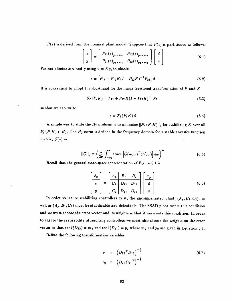
P(s) is derived from the nominal plant model. Suppose that P(s) is partitioned as follows:

y P21(s)p_xm,P22(s)p_x., u

We can eliminate u and y using u = Ky, to obtain

e= [e,,+ d (6.2)

Itisconvenient to adopt the shorthand for the linearfractionaltransformation of P and K

_'t(P, K) = P,I + PI2K(I - P22K)-I P21 (6.3)

so that we can write

e= 7, (P,K) d (6.4)

A simple way to statethe//2 problem isto minimize ll_t(P, K)ll2 for stabilizingK over all

-_'t(P,K) E H2. The//2 norm isdefined in the frequency domain for a stabletransferfunction

matrix, G(s) as

Recall that the general state-space representationof Figure 6.1 is

(6.5)

= C1 Dll D12 (6.6)

C2 D21 D22

In order to insure stabilizing controllers exist, the uncompensated plant, (Ap, B2,C2), as

well as (A_, B1, C1) must be stabilizable and detectable. The SSAD plant meets this condition

and we must choose the error vector and its weights so that it too meets this condition. In order

to ensure the realizability of resulting controllers we must also choose the weights on the error

vector so that rank(D12) = m2 and rank(D21) = P2 where m2 and p2 are given in Equation 6:1.

Define the following transformation variables

1

)-,zl -- D12

z2 = (D21D21 "') -J]

(6.7)

82

andapplythemto theplantasfollows

/_2 ---- B2 Zl

= z2C2

DI_ = D12zl

b21 = z2 D21

(6.8)

Let us assume these transformations have already been applied, thus D12 and D21 have

been normalized so that

D12=[0 I] 'r and D21 =[0 /] (6.9)

The point of these transformations is that we can reduce the complexity of the controller

formulas as long as we can write

and

D12"r [c1 D12] = [0 I] (6.10)

I01D2, 't' = (6.11)D_I I

Equation 6.10 means that the penalty on e = C1 zp+D12u includes a normalized, nonsingular

penalty on u. In other words, the error vector includes the control inputs with an identity

weighting matrix and there is no cross weighting between the states and the control.

Equation 6.11 is dual to Equation 6.10. This equation flows from assuming that the dis-

turbance vector, d, includes both the process noise on the states and the sensor noise on the

measurements. These noises are separate and the sensor noise weighting matrix is normalized

and nonsingular.

The transformations in Equation 6.7 allow us to choose non-normalized weights for D12 and

D21 and then scale the plant so that Equations 6.10 and 6.11 still hold.

83

Twoadditionalassumptionsmadeon theplantarethat D11 = 0 and D22 _ 0. We require

the former for the H2 cost to be finite; the latter simplifies the formulas. For SSAD D22 = 0

and we chose the error vector to not include the disturbance hence Dll = 0.

Thus the form of the system becomes

with

= C1 0 D12

C2 D21 0

D,2 =[0 I] '1' and D2, =[0 /]

(6.12)

Before proceeding, let us define some notation. Let A, Q, and R be real n x n matrices. Q

and R are both symmetric. Define the ttamiltonian matrix, H, as

H :- (6.13)Q -A 'r

The definitions of the symbols dom(Ric) and Ric(H) are that if H E dom(Ric) and X = Ric(H)

then

(i) X is symmetric.

(ii) X satisfies the algebraic Riccati equation

A'rX + XA+ XRX - Q = 0

(iii) A + RX is stable.

In order to find an admissible controller g which minimizes II_¢(P, g)l12, we must solve

the following two Riccati equations given by their ttamiltonian matrices

I A v - B2 B2 v' ]X.2 = Ric (6.14)

-C1 "1'C1 -AI, v"

Y'_ = Ric I -B,ApT'BI"'' -C2""C2]_Av (6.15)

84

Thetwosolutions,X2 and Y2, are positive semidefinite. Using these solutions, define

F2 = -B2"'X2 (6.16)

L2 = -Y2C_ 'r (6.17)

Notice that if the control weighting matrix is normalized to identity as we have done, F2 is

the optimal state feedback gain as solved for last in the Chapter with full state feedback. L2

represents the solution to the Kalman filter gain matrix. Now we may write the unique optimal

controller as

f 3

[ Ap + B2F2 Jr" L262 -L2 [ (6.18)K(s)

L F2 0 ]Considering that our plant is square, (six inputs and six outputs), we have an invertible

system A matrix, and that the non-minimum phase transmission zeros are fast relative to the

rest of the system, it is tempting to apply a loop-shaping technique. The Linear Quadratic

Gaussian/Loop Transfer Recovery (LQG/LTR) method presented in References [12] and [13] is

a loop-shaping technique that allows us to shape the singular values at the input or output of

the plant.

Unfortunately, in the LQG/LTR methodology, the ways in which the process noise and

sensor noise enter the plant are treated as tuning parameters rather than as representations

of the real plant behavior. In terms of Equation 6.6, B1 and D21 become design parameters

which are adjusted along with the weights on the states and the controls to shape the singular

values. For SSAD the process noise, Shuttle jet firings, does enter the system in a prescribed

manner. LQG/LTR can still be applied on SSAD, only it is not possible to directly shape the

singular values of interest. After initial attempts at applying LQG/LTR it became apparent

that conventional H2 allows a more direct approach the problem since B1 and D21 are physical

parameters.

85

6.2 H2 Results

In the H2 problem, the design parameters are the choice of weights on the contents of the

error vector, y and u. In SSAD, since y corresponds to the end effector states, we can choose the

C1 weights as we selected Q when designing a LQR. We multiply each channel corresponding

to an attitude by an order of magnitude to account for the difference between position and

attitude singular values in the open-loop system. In this manner a one inch error is not treated

as serious as a one radian error by the H2 controller. This choice is only an initial guess and

can be modified to bring the closed-loop system within performance objectives.

The weights on the control effort, D12, are initially placed at the inverse of the joint rate

limits as in the LQR design. Again, this design parameter is tuned until a satisfactory design

is achieved. One thing to note, the final weights of the H2 design do not have to correspond

to the final weights of the LQR design. Recall the differences between the two design plants;

LQR assumes full state feedback uncorrupted by noise while the H2 compensator has only the

observation vector which is also corrupted by sensor noise.

Section 6.2.1 examines the control effort and performance singular values of the H2 design.

A time domain simulation driven by the same jet firing pattern as used on the LQR is included

as well to help interpret the singular values. Section 6.2.2 examines the stability robustness of

the H2 design.

6.2.1 H2 Control Effort and Performance

Figure 6.2 shows the singular values from disturbance to each individual control effort

channel after tuning the weights on the error vector. As before, each control weight is fine

tuned until the scaled singular value falls just below one. Notice that two of the control effort

singular values actually lie below one. These are the singular values corresponding to elbow

pitch and wrist pitch joints.

During the design process, if a particular control effort singular value fell below one, the

corresponding weight was reduced allowing the compensator to use more control in that channel.

Conversely, if a control effort singular value fell above one, the corresponding penalty was

increased. For the elbow pitch and wrist pitch joint rates, the penalties were successively reduced

up until the weighting matrix, D12 started to numerically fail the rank tests. Nevertheless, the

86

Singular Values from Disturbance to H2 Control Effort10o

10-1

_ 10-3

I .10-5

10-6 _10-3 10-2 10-1 100 101 102

Frequency (radians/second)

Figure 6.2. Control Effort Singular Values of the H2 System

compensator chose not to use more control in these channels.

There are two explanations for this result. First, the elbow pitch and wrist pitch joint rates

may have limited ability to affect the performance objectives. Consider the simple example of a

body with horizontal and vertical velocity as its controls. If we choose as performance objectives

vertical position only, a controller would have no reason to use the horizontal control channel.

This seems unlikely for SSAD since clearly from Figure 6.2 it is using some control in these

channels. If the penalty is made less on these channels, it should use more control even if the

benefit is slight. A more likely explanation is that use of the elbow pitch and wrist pitch joint

rates is penalized through some coupling in the system. Use of elbow pitch may, for instance,

reduce the error in the X direction but cause large excursions in Y which would require use

of shoulder pitch to compensate. Thus the weight on shoulder pitch indirectly penalizes elbow

pitch as well.

Figure 6.3 presents the singular values from disturbance to end effector position and attitude.

Included on the same plots is the corresponding information for the open-loop system. For the

/-/2 design we are barely able to meet the performance goal of less than 1 inch excursion in

position. We are able to meet the attitude goal of less than 0.01 radians of rotation excursion

87

101

10-1

10-2

10-3

10-5.*'M.

10-6

10-710-3

10-1

r_

t:.,i10-3

:_ 10-5

o 10-6

10-7

10-8'10-3

Singular Values from Disturbance to End Effector Position

10-2 10-1 10o 101 102

Frequency (radians/second)

Singular Values from Disturbance to End Effector Attitude

10-2 10-1

"X

.....i& .....i'd',.....ieFrequency (radians/second)

Figure 6.3. Performance Singular Values of the H2 System

88

without problem. Both goals are met without exceeding the joint rate limits.

As with the LQR design, to help visualize what is occuring on the singular value plots, a

time domain simulation is presented in Figures 6.4 and 6.5. These Figures include both the

response of the open-loop system and the H2 system. As before, a roll command is given for

a full 10 seconds immediately followed by a 10 second pitch command and finally a 10 second

yaw command.

From Figure 6.4 we can see that as in the LQR design, the X direction has considerably

poorer disturbance rejection than the Y and Z directions for the H2 compensator. Similar

improvement over the uncompensated system as in the LQR design is also apparent. For the

attitude directions, roll disturbance rejection is considerably better than the other axes as shown

in Figure 6.5. Overall, the resulting H2 design performance is only slightly below the full state

feedback LQR design.

6.2.2 H2 Stability Robustness

Applying both the small gain test and p-analysis to the closed-loop H2 system results in

Figure 6.6. As before, the system fails both stability robustness tests. With the LQR plant, we

evaluated the eigenvalues of the closed-loop system for four sets of the parameters and showed

that the system was stable for these endpoints. Though this is not conclusive proof, it suggests

that it is possible that the LQR closed-loop system is indeed robustly stable.

Evaluating those same sets of parameters for the closed-loop H2 design does show conclu-

sively that the system is robustly unstable. Figure 6.7 shows the near pole locations for the

nominal closed-loop H2 system. The following four Figures show the closed-loop poles for the

four sets of perturbed parameters. Figure 6.8 places both the K_tA and the K(; at their mini-

mum values. Figure 6.9 places both sets of parameters at their maximum values. Figure 6.10

places the KMA at their minimum values and the K(; at their maximum values. Finally, Fig-

ure 6.11 considers the last permutation of the KMA at their maximum values and the K(_ at

their minimum values.

Aside from the nominal plant, the closed-loop system is only stable for Figure 6.9. In

Chapter 4 when considering the open-loop plant, we were able to isolate the stability problem

to when the system is operating at very low amplitudes. In this region, K_A is at its maximum

and K_,; is near its minimum. For the H2 system we cannot draw the same conclusions. Stability

89

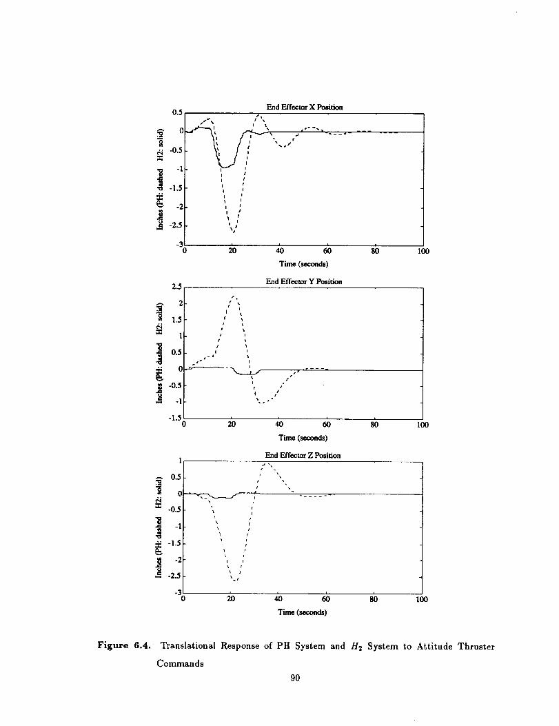
End EffectorX Position0.5. ,.

¢s_% I s

-_ -11- ?'_ '

"_ -1.5

_ -2

-2.5

-30

I ¢

I t

I tI

'j ,,I

I I

I r

i i

_jJ

_ 6bTime (seconds)

I00

2.5End Effector Y Position

1.5

0.5

o-0.5

r

?

I

f

/s_j I

-',,.,._./

t"

I t

-1.5 o io 4_ 6_ 8bTime (seconds)

100

End Effector Z Position

,-, 0.5

0

:_ -0.5

g"O

-I.5

-2.5

s

i

t

i_t i

jt

x

-3o _o _o _ sb .00

Time (seconds)

Figure 6.4. Translational Response of PH System and H2 System to Attitude Thruster

Commands

90

0.01End Effoctor Attitude: Roll

_ 0.005

6im 0

._0.005

_-0.01

.i[0.015

-0.020

js _%

I

?

1I

1

X

io

1

Time (seconds)

m

.i

0

-5

-10

-15

10-3 End Effe_tor Attitude: Pitch

pP_l.

_- _ Itf • • _ - _ - _ _ ° _.

I

II !I

I,t

2°o io _o _ sbTime (seconds)

0.0_

A

0.01. _

6i

._ O.Ol

End Eff_tor Attitude: Yaw

/ I

I

0.005 [- ;

I :,--/x ', ..J oL /

0 20 40

100

100

60 80 100

Time (seconds)

Figure 6.5. Rotational Response of PH System and H2 System to Attitude Thruster Com-

mands

91

102 H2: Small Gain Test (solid) Mu-Analysis(dashed)

10]

10o

10ol

x

i

100"1:z003..... "l'ff2 ..... .1'ffl ..... '1'_ .... '1"()'1 ..... '1'62

Frequency (radians/second)

Figure 6.6. Robust StabilityAnalysisof the H2 System

H2 Closed-Loop Near Poles for Nominal Plant

2

0

-2

X

-6

X

........................................................................................

X

X x X

x _...... X ............................................ X ................. "X .... X -'........ X- ")U_IK-

×' X X

....................................................................... X": ...... X .....X

-6 -5 -4 -3 -2 -1 0

Real

Figure 6.'/.Closed-LoopPolesofthe Nominal H2 System

92

0

-2

-4

H2 Closed-Loop Near Poles for Nominal Plant Kma at min, Kg at min)6 .

x

............... , ............... , ............... , ............... ,'.

×

x- ............................

X XX

.............. ................ . .............................. X ....... X" - lll&t- _- ............

X Xx _k

X

.............. ,- .............................................. ,- ............................

x

-6-5 -4 -3 -2 -1 0

Real

Figure 6.8. Closed-Loop Poles of the Off-Nominal H2 System: 1

H2 Closed-Loop Near Poles for Nominal Plant Kma at max, Kg at max)6

......................................................... X ..............................

Xx

....... . ......... , ......... . ....... , ........ , .......... . ......... , .......... ,...x ....

x x

x Xx0 ......................-x...............x:..........................x-............x-._--II,_4-

X .Xx

X X

X

X

4 .......... •.......... ,.......... •.......... •.......... ........... •.......... ........... ,..........

x

-6-4.5 -4 -3.5 -3 -2.5 -2 -1.5 -1 -0.5 0

Real

Figure 6.9. Closed-Loop Poles of the Off-Nominal H2 System: 2

93

6 H2 Closed-Loop Near Poles for Nominal Plant (Krna at rain, Kg at max)

I x4 --x .................................................. : .....................................

a

2

0

-2

-4

-6

• X

................................................... i ........ X'" " : ...... X .................

x x:x X

:X X X_(

................................................... ! ........ x... ; ...... X.................

X : x

X

-6 -5 -4 -3 -2 -1 0 1

Real

Figure 6.10. Closed-Loop Poles of the Off-Nominal H2 System: 3

0

-5 -4 -3 -2 -1 0

Real

Figure 6.11. Closed-Loop Poles of the Off-Nominal H2 System: 4

94

is aproblemfor theclosed-loopsystemin severalconfigurations.If the stability problemwas

causedby neglecteddynamics,asolutionto robuststabilitywouldbe to reducethebandwidth

of the system.This couldbeaccomplishedby eitherfurther penalizingthe controleffort or

reducingthe weightson theendeffectorstates,ie.,demandlessperformance.Unfortunately,

withparametricuncertaintythe lowfrequencysystempolessimplyaren'twherethecontroller

is expectingthem. Reducingthebandwidthwill notsolveourproblem.Wewill explorethis

issuein furtherdetailwhenconsideringtheH_ design.

6.3 Summary

This Chapter removes the requirement for full state feedback uncorrupted by noise and

presents the /-/2 (or LQG) approach. This approach involves designing a Kalman filter to

estimate all of the system states from the observation and control vector and then using these

estimates as perfect state information fed into a LQR.

On the nominal plant, the/-/2 approach is able to recover performance comparable to the

LQR design. Both performance objectives are met without exceeding the limits on the control

effort. Unfortunately, the closed-loop/-/2 system is not robustly stable in face of the parametric

uncertainty present in the plant as indicated by both p-analysis and the small gain test. Though

these tests are both conservative for real parametric uncertainty, eigenvalue analysis shows

conclusively that the system is not robustly stable.

95

Chapter 7

Hoo Design

In the last Chapter we designed a compensator that meets performance specifications within

allowable control effort specifications by minimizing the//2 norm of the transfer function from

exogenous inputs to the error vector. This Chapter solves a similar problem, only this time

performance is measured with an Hoo norm. The Hoo norm is defined in the frequency domain

for a stable transfer function matrix as

IIG( )II = sup _'[G(jw)]

Ilyl12= sup (7.1)

Ilull2

Using this norm, an Hoo optimization design technique will result in the compensator that

minimizes the supremum over all frequencies of the maximum singular value of the transfer

function of interest.

Recall that the disturbances acting on the SRMS are caused by Shuttle attitude thruster

firings. The Shuttle may fire its thrusters in pulses every 80 milliseconds, or for steps lasting as

long as 200 seconds. Such a firing profile has the ability to excite the system at any frequency

up through its bandwidth. This makes the Hoo norm a natural selection for optimization. We

would like to reduce the worst case gain for disturbances of the SRMS at all frequencies.

There are many parallels between the H2 and Hoo approaches. Development of the Hoo

theory in Section 7.1 flows naturally from the work of last Chapter. As in the H2 case, we

arrive at two algebraic Riccati equations. The Hoo Riccati equations can be thought of as

those that arise from a linear quadratic differential game between two opposing players. One

player chooses the disturbance to maximize the norm of the output while the opposing player

96

e

Figure 7.1. Plant With Compensator

chooses the control input to minimize it. The work in this Section follows that of Reference [17].

Though not presented, the Hoo design technique can also be derived by recasting the system as

a model-matching problem via the parametrization of all stabilizing controllers. An exposition

of this technique is presented in Reference [18].

Section 7.2 analyzes the results of the Hoo design using the same criteria as in previous

Chapters. The singular values from disturbance to control effort and disturbance to the end

effeetor states are examined and compared to the open-loop system. To highlight the differences

in optimizing the H2 norm versus the Hoo norm, a comparison of these two designs is presented

as well. As before, a time domain simulation of the same jet firing pattern is presented.

Finally, stability robustness of the closed-loop Ha system is examined in face of the parametric

uncertainty. By choosing a different transfer function to optimize, namely the output of the

plant uncertainties to the input of the plant uncertainties, we can determine if any Hoo controller

would be able to robustly stabilize the plant.

7.1 Hoo Theory

For the Hoo design we will use the same general two-block diagram as shown in Figure 7.1.

Define the error vector the same as for the H_ design, namely

Using the same notation as in the last Chapter, write the transfer function from the exogenous

inputs to the error vector as

97

e = 7, (p, K) d (7.2)

The Hoo optimal compensator is the compensator that minimizes the supremum over all

frequencies of the maximum singular value of Yt (P, K) for stabilizing K. This can be written

a_

min 117t (P, K)lloo= rain sup _(._'t (p, K) (j_)) (7.3)stabilizing K stabilizing K ,,

In practice however, contrary to the H2 problem, H_ optimal controllers are more difficult to

characterize than suboptimal ones. We settle for an admissible K such that II_t (P, K)lloo < "r-

Before characterizing the H_ suboptimal controllers, consider the transfer function matrix

of Figure 7.1 to be in the same form as the H2 problem. That is

with

["_L-yr} [ Ar I B1 B2= Gt 0 D12

6'2 D21 0

D+2-[0 I] 'v and D2+ =[0 /]

Hoo theory requires that the following must hold true for the system:

(a) (A, B1,6"1 ) is stabilizable and detectable.

(b) (A, B2, 6"2) is stabilizable and detectable.

(¢) D,2 "t'[C, Dr2] = [0 /].

,d,I [°}°2

(7.4)

The weights on the states in the error vector, e, must be chosen to insure (a) is met. As

shown in Chapter 4, (b) is known to be true for SSAD. To meet conditions (c) and (d) it will be

necessary to apply the same transformations on the system used in the H2 problem as shown

in Section 6.1. Implicit in the given state-space realization for Figure 7.1 is that Dll = 0

and D22 = 0. In a general Ho_ problem these conditions can be relaxed, though it would

98

complicate the formulas presented here considerably. A treatment of the more general problem

can be found in Reference [19].

The H_ suboptimal problem is to find an admissible K such that 117,(P, K)II, < 7. its

solution involves two I-Iamiltonian matrices as in the H2 problem

Ap 7-2B1 B1 'r _ B2B2'r I

3

F_ = (7.5)-C1 'rc1 -A_, 'r J

[ A/"r 7-2C1 'rc1 - c2'rc: ] (7.6)Joo

L-B1 B1 'r _A T J

These Hamiltonians are remarkably similar to the //2 formulation. The main difference is

that the additional terms in the upper-right entry of both Foo and Joo make the two Hamib

tonians no longer sign definite. Therefore we cannot guarantee that either Foo or Jo_ has a

Riccati solution "or that the solution is positive definite. In fact, this limitation is related to the

existence of a Hoo suboptimal controller.

In Reference [17], Doyle et al prove that there exists an admissible controller, K, such that

II_'_ (P, g)ll_ < 7 iff the following conditions hold true

(i) Foo 6 dom(Ric) and X,_ := Ric(F,_) > 0.

(ii) J,_ 6 dom(Ric) and Y,_ := Ric(J,_) > 0.

(iii) p(X_Y_) < 72 where p(M) is the spectral radius of M.

When all three of these conditions hold, one such suboptimal controller is

[a'l'"K_,(s) := (7.7)C_ 0

where

Ao_ = A T + 7-2BiB1'rxoo + B_Coo - BooC2

Boo = (I - 7-2YooX_)-'YooC2 '''

Coo = - B2"I'X oo

(7.8)

99

Conditions(i) through(iii) suggestthefollowing method, known as 7 iteration, to calculate

an Hoo 'optimal' controller: select a positive number 7; test conditions (i) through (iii); increase

7 if failed or decrease 7 if passed; repeat until within a desired tolerance.

To illustrate the relationship between the Hoo and H2 solutions, notice that as 7 --" oo,

Xoo --" X2, etc., and Koo -" K2. This can be seen directly from the two sets of Hamiltonians

in the Hoo and H2 problem formulations; as 7 -" oo the Hoo Itamiltonians become the H2

Hamiltonians.

7.2 H_o Results

As in the//2 problem, the design parameters of the Hoo problem are the choice of weights

on the contents of the error vector, namely y and u. In design, select the C1 weights for the Hoo

problem as before when designing both the /-/2 and LQR controllers. That is, multiply each

channel corresponding to an attitude by an order of magnitude to account for the difference

between position and attitude singular values of the open-loop system. This is to ameliorate

the difference between a one inch error and a one radian error.

The weights on the control effort, D12, are treated as the main tuning parameter. The

weight on each control channel is increased or decreased appropriately until every control effort

singular value does not exceed the corresponding joint rate limit. The final weights of the Hoo

design need not correspond to the weights of the /'/2 design since a different norm is being

optimized.

Section 7.2.1 examines the control effort and performance singular values of the Hoo design.

The performance singular values are compared not only to the open-loop plant but also to the

//2 design in order to highlight the differences in the two design techniques. A time domain

simulation driven by the same jet firing pattern used on the other designs is included as well to

help interpret the singular values. Section 7.2.2 examines the stability robustness of the /-/oo

design. By choosing a different transfer function's Hoo norm to minimize, we can determine if

it is possible to design a robustly stable compensator.

7.2.1 Hoo Control Effort and Performance

Figure 7.2 shows the singular values from disturbance to control effort after tuning the

100

100

10-1

10-2

10-3

Singular Values from Disturbance to H-inf Control Effort

10-4 ' ................................10-3 10-2 10-' i'(_ i'6'1 i'02

Frequency (radians/second)

Figure 7.2. Control Effort Singular Values of the Hoo System

weights on the error vector. As before, each control channel weight residing in D12 is fine tuned

until the scaled singular value falls just below one.

In the/-/2 solution, the controller did not make full use of every control channel, specifically

elbow pitch and wrist pitch. For the Ho_ design a different norm is designed for, the Hoo norm,

that is the supremum over all frequencies of the maximum singular value, not the area under

the singular value curves as in the H2 case. The Hoo controller is able to make use of each

control to its full potential since it is penalizing the control channels in a different way.

Figure 7.3 presents the singular values from disturbance to end effector position and attitude.

Included on the same plots is the corresponding information for the open-loop system. The

Hoo design is able to meet the performance goals of less than 1 inch excursion in position and

less than 0.01 radians of rotation excursion without exceeding the joint rate limits.

Figure 7.4 compares the singular values from disturbance to end effector position and at-

titude for both the Ho_ and /-/2 systems. Because the H_o design is trying to minimize the

Hoo norm, it has sacrificed some performance at 2 rps so that the maximum singular value can

be brought down. The difference between the two designs is not as dramatic as can be seen

in other systems since the /-/2 design does not contain any large resonances, or 'hills,' in its

101

101

o 10o

•_ 10-1• !

10-2

10-3

1_17_3 ..... '1"_2

Singular Values from Disturbance to End Effector Position

-- --___%

..... '1'{_1 ..... 'I'{_) ..... '1'61 ..... '1'02

Frequency (indians/second)

10-1

om 10-2

10-3

"_ 104

10-5

._ 10-6

_ 10-7

10-8,10-3

Singular Values from Disturbance to End Effector Attitude

_X

Frequency (radians/second)

Figure 7.3.PerformanceSingularValuesofthe Hoo and PositionHold Systems

102

10o

o 10-1

10-2

104

._ 10-5

_ 10-6

10-710-3

Singular Values from Disturbance to End Effector Position

..... 'l'ff2 10-1 100 101 102

Frequency (indians/second)

O

,M

Singular Values from Disturbance to End Effector Attitude10-2 ...............................

10-3

10.4

10.5

--- 10.6

_ 10.7

3 10.2

....

..... '1'61 ..... .1'1_) .... .1'0'I ..... "1'02

Frequency (radians/second)

Figure 7.4. Performance Singular Values of the Hoo and H2 Systems

103

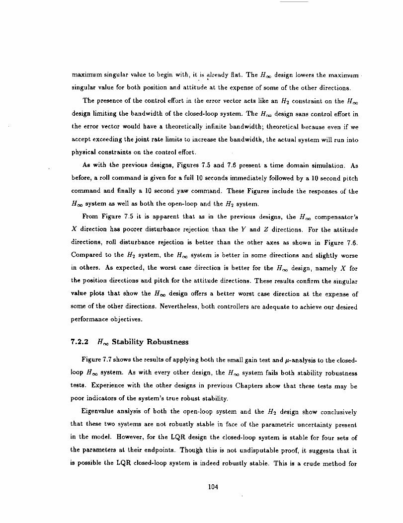
maximum singular value to begin with, it is already flat. The H_ design lowers the maximum

singular value for both position and attitude at the expense of some of the other directions.

The presence of the control effort in the error vector acts like an H2 constraint on the H_

design limiting the bandwidth of the closed-loop system. The Hoo design sans control effort in

the error vector would have a theoretically infinite bandwidth; theoretical because even if we

accept exceeding the joint rate limits to increase the bandwidth, the actual system will run into

physical constraints on the control effort.

As with the previous designs, Figures 7.5 and 7.6 present a time domain simulation. As

before, a roll command is given for a full 10 seconds immediately followed by a 10 second pitch

command and finally a 10 second yaw command. These Figures include the responses of the

Hoo system as well as both the open-loop and the/-/2 system.

From Figure 7.5 it is apparent that as in the previous designs, the Hoo compensator's

X direction has poorer disturbance rejection than the Y and Z directions. For the attitude

directions, roll disturbance rejection is better than the other axes as shown in Figure 7.6.

Compared to the H2 system, the H_ system is better in some directions and slightly worse

in others. As expected, the worst case direction is better for the H_ design, namely X for

the position directions and pitch for the attitude directions. These results confirm the singular

value plots that show the H_ design offers a better worst case direction at the expense of

some of the other directions. Nevertheless, both controllers are adequate to achieve our desired

performance objectives.

7.2.2 Ha Stability Robustness

Figure 7.7 shows the results of applying both the small gain test and p-analysis to the closed-

loop Ha system. As with every other design, the Ha system fails both stability robustness

tests. Experience with the other designs in previous Chapters show that these tests may be

poor indicators of the system's true robust stability.

Eigenvalue analysis of both the open-loop system and the H2 design show conclusively

that these two systems are not robustly stable in face of the parametric uncertainty present

in the model. However, for the LQR design the closed-loop system is stable for four sets of

the parameters at their endpoints. Though this is not undisputable proof, it suggests that it

is possible the LQR closed-loop system is indeed robustly stable. This is a crude method for

104

°:1,_ _0.5I

-1¢,q

•. -1.5

_ -2_ -2.5

-30

2.5

2._ 1.5

1

¢q 0.5

o___ -0.5

'_ -1

-1.50

1

o.5

._, 0

... -0.50

_ °1

._. -1.5

g -2-_ -2.5

-30

End Effector X Position

'g.,

* \

I

i!

Il

I

I

iI

I

t

I

tu---_,b

f

1o _o 6b 8bTime (seconds)

End Effector Y Position

r 1

t ¢ s,I

I

t

I I

fI ,

/

20 _o

Time (seconds)

s_

End Effector Z Position

i xx

x

I

\

1

rI

it

_o _o 6b 8bTime (seconds)

I00

I00

O0

Figure 7.5. Translational Response of PH, H2, and Hoo Systems to Attitude Thruster Com-

mands

105

0.01End Effector Att/tud¢: Roll

_ 0.005.°t_

-- 0

_0.005

._. -0.01

_B-O.O15

a.m

-0.020

t

1I

'l

I

/o

L

I

4b d sbTime (seconds)

IO0

5x 10-3 End Effector Attitude: Pitch

I _,

•. 0 _ .. ..... ____

-10

-15

-200

I ". ., f

,," t

t t !

, /

20 _o 6bTime (seconds)

gb IO0

0.02End Effector Attitude: Yaw

A

.-a_0.015

.,_

_ 0.01tPl

-_ 0.005

-0.005

r.,-- i s-

._t"

_x\jt

o _o _o _ _ lOOTime (seconds)

Figure 7.6. Rotational Response of PH, H2, and Hoo Systems to Attitude Thruster Commands

106

102H-inf: Small Gain Test (solid) Mu-Analysis (dashed)

101

"_ 10O

10-1

\x _ _

\

\

a t i L i .... , , , Li,tll t i .... ,,I , , i i i10.2 10., loo '1'6',Frequency (radians/second)

..... '1'02

Figure 7.7.Robust StabilityAnalysisof the Ho_ System

examining robust stability; however the nature of our system leaves few options. Though the

Hoo system fails both stability robustness tests, let us examine the eigenvalues of the closed-loop

system at certain endpoints of the parameters as before.

Figure 7.8 presents the near pole locations for the nominal closed-loop Hoo system. The

following four Figures show the closed-loop poles for the four sets of perturbed parameters.

Figure 7.9 places both the KMA and the Kc'i at their minimum values. Figure 7.10 places both

sets of parameters at their maximum values. Figure 7.11 places the KAvA at their minimum

values and the Kt_ at their maximum values. Finally, Figure 7.12 considers the last permutation

of the KAvA at their maximum values and the Kt_ at their minimum values. Evaluating these

sets of parameters for the closed-loop Hoo design, as performed for the LQR and H2 systems,

shows conclusively that the system is indeed not robustly stable.

Aside from the nominal plant, the closed-loop system is only stable for system 2 shown in

Figure 7.10. This is also the case for the H2 system considered in Chapter 6. Similar to the

/-/2 plant, it is not possible to draw any conclusions for the Hoo system about certain regions

of operation that are causing instability since stability is a problem for several configurations.

If the stability problem was caused by neglected dynamics, a solution to robust stability

107

3 H-inf Closed-Loop Near Poles for Nominal Plant

t_

2

0

-1

-2

XxX

x................................................................... X. ......................

X X

X

_- ............................ _()o_- -X-X- -

x

x X

x

X xx

............................................ X- .......................... X ..............

X

-321.5 -2 - 1.5 -1 -0.5 0

Real

Figure 7.8. Closed-Loop Poles of the Nominal Hoo System

H-inf CL Near Poles (Kma at min, Kg at min)

-1

x

..........................................................................................

X

x ......... , .............

X

.....X- ........ :......... X-....:............ X ......... X .....:......_ ....:lillE-'.-.............

., .. : "" X: _

X

x-3 ...........................................................................................

-4 x-5 -4 -3 -2 -1 0

Real

Figure 7.9. Closed-Loop Poles of the Off-Nominal Hoo System: 1

108

H-inf CLNearPoles (Kma at max, Kg at max)

3

2

1

0

-1

-2

-3

-4-3

X Xx '

............................................................................ '.'")4...... D_- --X

X X........... N: ...... I_-_- -

X .x

X :X • x

X

x

.............. • ............... •................. X

i

-2.5 -2 •.5 - -0.5 0

Real

Figure 7.10. Closed-LoopPolesof theOff-NominalHoo System: 2

4H-inf CL Near Poles (Kma at min, Kg at max)

x:_ ..............................

X

2 ......................................................... xi ........ x .................

X :. X X iX

. X

'0 .......... "X ................... X ................ X .... )_ "X..... X" "X)IK': ...............

:_ .

X] ......................................... i...............

.It ............................... '.... '. x x×

-2 ............... ,............... , ........................... X: .......... -X-- -:..............

'X-3 .............. i............... i.............................. i............... i..............X:

-4-5 -4 -3 -2 -1 0

Real

Figure 7.11. Closed-LoopPolesof the Off-NominalHa System: 3

109

4 H-mf CL Near Poles (Kma at max, Kg at mm)

3

2

×

0

-1

-2

-3

--4

-5

.............. . ............... . ............... . ............... _ ............... . ..............

×

X

! x:

.... x- ................. ×- ................ x.i ........ _ ..... ...... _ .... _-i ._- ............1

×:_

x

×

×

-4 -3 -2 - 0

Real

Figure 7.12. Closed-Loop Poles of the Off-Nominal Hoo System: 4

would be to reduce the bandwidth of the system. Unfortunately, with parametric uncertainty

the system poles simply aren't where the controller is expecting them. Reducing the bandwidth

will not solve the problem. Chapter 4 shows that the open-loop system itself is not robustly

stable in face of the parametric uncertainty present. Therefore even a zero as the transfer

function for the controller will not stabilize the plant. However, using the Hoo design process

it is possible to design for robust stability directly to see if it is achievable for the SSAD plant.

Recall the general three block formulation shown in Figure 7.13 and its closed-loop repre-

sentation shown in Figure 7.14. G(s) is the closed-loop transfer function which combines the

dynamics of the plant and the compensator. Recall that the closed-loop transfer function, G(s),

can be divided into a set of four transfer functions as follows,

i ]:ic11 ,] 79,e O2;(s) O22(s) d

Chapter 4 shows that if IIGll (s)lloo < 1, robust stability is achieved via the small gain test.

Therefore, the Hoo design process will design for robust stability directly with no consideration

for performance if the input and error vectors are chosen such that the transfer function from d

110

U

eI

Figure 7.13. Standard Form for a Compensated Plant with Uncertainty

eI

Figure 7.14. Closed-Loop Transfer Function

111

to e is Gll (s). The Hoo design methodology will try to minimize the Hoo norm of this transfer

function. If it can bring the maximum singular value below one, by the small gain test robust

stability is guaranteed.

Before proceeding on this robust stability design, there is a subtlety to consider. In order

to insure that the rank conditions outlined in Section 7.1 are not violated, the exogenous input

vector, d, must include not only the output of the uncertainty block 77, which replaces the

process noise, but must also include the sensor noise. Similarly, the error vector e must include

u as well as e. These are conditions (c) and (d) from Section 7.1. Hence,

The subtlety is that if u is penalized by being included in the error vector, the ability to achieve

robust stability is also penalized since it may require large amounts of control. Remember

that for now, performance is not considered at all, the only concern is to see if any controller

can robustly stabilize the system 1. Therefore, the design process to achieve a robustly stable

compensator is to decrease the penalty on u until the maximum singular value of the closed-loop

system falls below unity.

After decreasing the weight on the control channels to 10 -1° , the plant starts to numerically

fail the rank tests. Unfortunately, at this point the plant still fails to achieve robust stability.

Figure 7.15 presents the results of both the small gain test and p-analysis on this 'Gl1' Hoo

design. Though robust stability is not achieved, the curves are at their lowest levels out of

every design, including the open-loop system. However, do not think of this system as less

robustly unstable since robust stability is a binary test that this design fails. Even this attempt

at robust stability has come at enormous cost.

Recall that this design gives basically no regard for performance whatsoever. Figure 7.16

shows the scaled singular values from disturbance to control effort. The joint rate limits have

been exceeded by almost five orders of magnitude. Figure 7.17 presents tlie singular values

from disturbance to end effector position and attitude. Clearly, the price is quite high in the

effort to achieve robust stability. Unfortunately the goal is not even achieved.

1The I,QR system i_ robustly stable, but it requires fidl-stat, e feedback

112

102Small Gain Test (solid) Mu-Analysis (dashed)

, ....... , , ..... , , . , . ,,.

i

101

10o

10q

...... i& ...... ib'_

Frequency (radians/second)

102

Figure 7.15. Robust Stability Analysis of the 'Gl1' H_ System

109

lOS

103

10-3

Singular Values from Disturbance to Control Effort

i , . , , ,,,., , . , , , .... , . ......... , , ..... , . , .... , , . .,,

10-610-4 .... i&, ..... i& ..... i& ..... i6; ..... i6_ ..... io=

Frequency (radians/second)

Figure 7.16. Control Effort Singular Values of the 'Gl1' Hoo System

113

1011Singular Values from Disturbance to End Effector Position

, , , ,,, ........... , ....... , , ,,,,, ............... .

10s

105

"_ 102

10-1

10-4

10710-4

............ , ,,i.. J ,,,,L,, . , ....... _ t t ttllll i i , itlJ

10-3 10-2 10-1 100 101 102

Frequency (radians/second)

1010 - . Singular Values from Disturbance to End Effector Attitude• , , ..... • , ,,,,,, ....... , • ........... ,,,, .... ,,7

107

10-5

Frequency (radians/sec0nd)

Figure 7.17. Performance Singular Values of the 'Gl1' Hoo System

114

7.3 Summary

This Chapter presents a method for finding H_ optimal controllers that minimize, to a

desired tolerance, the H_ norm of the transfer function from disturbance to error vector. This

problem is closely related to the H2 design process which is minimizing the H2 norm of the

same transfer function. Both techniques involve a two Riccati equation solution process. Both

remove the requirement for full state feedback uncorrupted by noise called for in the LQR

design.

With the Hoo approach, on the nominal plant we are able to achieve performance better

than the H2 design. Performance is better in the sense that the worst case direction is of

less magnitude than the H2 design; however, this came at the expense of some of the other

directions. Nevertheless, both performance objectives are met without exceeding the limits on

the control effort.

Unfortunately the closed-loop Hoo system, like the H2 system, is not robustly stable in face

of the parametric uncertainty present in the plant. As before both /a-analysis and the small

gain test as well as actual eigenvalue analysis confirm the results. In an effort to achieve a

robustly stable design, the problem is recast to minimize the H_ norm of the Gll transfer

function. This essentially abandons all performance desires and tries only to achieve robust

stability. This process fails to achieve robust stability as well.

115

Chapter 8

Conclusions

Three regulator designs were developed to improve the performance of the Space Shuttle

Remote Manipulator System (SRMS). Designs focused on the Position Hold function of the

SRMS. Position Hold is universal to normal operations of the SRMS. In Chapter 2, the SRMS

system was examined in greater detail. A linear model of the nonlinear plant was developed

in Chapter 3. Two of the significant nonlinearities were modelled as parametric uncertainties

in an effort to capture their effect on the system. The linear model was compared to a higher

fidelity nonlinear model in the time domain.

In Chapter 4, the characteristics of the open-loop plant were explored. Because of the

numerical problems associated with six integrator poles, subsequent regulator designs used

the current Position Hold system as the open-loop plant. In this manner, the current system

moved the integrator poles off the jw-axis. In effect, the new designs operate as stability and

performance augmentation around the current system. Model reduction was applied to the new

open-loop plant.

The performance and control effort of the open-loop system were presented in Chapter 4 as

a baseline with which to compare subsequent regulator designs. The performance and control

effort criteria were analyzed in the frequency domain by looking at three sets of singular values:

disturbance to control effort, disturbance to end effector position, and disturbance to end effec-

tor attitude. A typical Shuttle attitude control jet firing pattern, which acts as a disturbance

on the system, was simulated in the time domain.

Also in Chapter 4, a sufficient condition for robust stability was developed using the small

gain theorem with an Hoo norm. The structured singular value, p, was defined and shown to

116

provide a necessary and sufficient condition for robust stability. In calculation, /_-analysis is

reduced to a sufficient condition, but it is less conservative than the small gain test. Unfortu-

nately these tests are conservative for lightly damped systems with real parametric uncertainties

- the exact description of the SRMS model. Application of these tests on the current system

determined it to be unstable. As confirmation, the eigenvalues of the system were calculated

for certain values of the uncertain parameters. For conditions corresponding to low amplitude,

slow motion, the current system was found to indeed be unstable. This corresponds to the slow,

low amplitude limit cycling observed in the actual system.

A Linear Quadratic Regulator (LQR) was designed in Chapter 5. Its performance and

control effort were a considerable improvement over the current system. Though the LQR

failed both the small gain test, and/_-analysis, actual eigenvalue analysis seemed to indicate

that the system may be robustly stable. Unfortunately this cannot be proved unequivocally.

Since full-state feedback is not available on the SRMS, two model based compensators were

designed.

In Chapter 6 the H2 technique and in Chapter 7 the Ha technique were presented. There

are many parallels between these two techniques. In both, an error vector is constructed from

the controls and some linear combination of the states. As the name implies, the H2 technique

designs an optimal compensator that minimizes the H2 norm of a transfer matrix using only the

system measurements. Similarly, the H_ technique minimizes the H_ norm. Both designs were

able to improve the performance of the nominal system considerably. However, neither design

achieved robust stability. Not only did both designs fail the small gain test and p-analysis, but

actual eigenvalue analysis showed the systems were indeed not robustly stable.

In an effort to achieve a robustly stable design, In Chapter 7 the problem was recast to

minimize the Ha norm of the Gll transfer function. By the small gain test, if the Ha norm

of this transfer function falls below one, robust stability is assured. This essentially abandons

all performance desires and tries only to achieve robust stability. Unfortunately, this process

fails to achieve robust stability as well. This modified design did establish the trade-off present

in the pursuit of robust stability at the expense of performance and control effort.

If the stability problem was caused by neglected dynamics, a solution to robust stability

would be to reduce the bandwidth of the system. This could be accomplished by either further

penalizing the control effort or reducing the weights on the end effector states, ie., demand

117

lessperformance. Unfortunately, with parametric uncertainty the low frequency system poles

simply aren't where the controller is expecting them. Reducing the bandwidth will not solve

the problem. Considering the open-loop system itself is not robustly stable, even a zero for the

compensator will not make the system robustly stable.

A possible extension for this thesis would be to gain schedule the controllers over certain

regions of the nonlinearities. In this manner, the uncertainty of the parameters would be reduced

allowing a family of controllers to be robustly stable over their respective regions. A 'real p-

analysis' technique would aid the design process allowing for the removal of conservatism in the

gain scheduled controllers. Additionally, the model can be modified to incorporate acceleration

sensors or optical measurements to provide for different measurements when NASA chooses a

new sensor suite.

The SRMS model suffers from lightly damped poles that have large real parametric un-

certainty. To achieve a single robustly stable design a 'real p-synthesis' technique is needed.

This technique must not only use the information of the structure of. the uncertainty, but also

account for exclusively real perturbations. The SRMS plant is an ideal candidate for a real"

p-synthesis technique.

118

Bibliography

[1] Gilbert, M.G., Scott, M.A. and Kenny, S.P., "Active Damping Application to the Shuttle

RMS," Fourth NASA/DOD CSI conf., Orlando, FL, 1990.

[2] Ravindran, R. and Doetsch, K.H., "Design Aspects of the Shuttle Remote Manipulator

Control," Proceedings of the Guidance and Control Conference, AIAA Paper No. 82-1581,

1982.

[3] McLean, D.D. and Girling, K., STS-3 Remote Manipulator System Press Kit, SPAR

Aerospace Limited, 1982.

[4] Nguyen, P.K., Ravindran, R., Cart, R. and Gossain, D.M., "Structural Flexibility of the

Shuttle Remote Manipulator System Mechanical Arm," Proceedings of the Guidance and

Control Conference, AIAA Paper No. 82-1536, 1982.

[5] Logan, B.A., Jr., "Shuttle Payload Deployment and Retrieval System," Proceedings of the

Guidance and Control Conference, AiAA Paper No. 82-1580, 1982.

[6] Newsom, J.R., Layman, W.E., Waites, ll.B. and Itayduk, R.J., "The NASA Control-

Structures Interaction Technology Program," Proceedings of the _Ist Congress of the In-

ternational Astronautical Federation, IAP Paper No. 90-290, 1990.

[7] Barrows, T.M., A Simplified Simulation for the Analysis of Heavy Payloads on the Shuttle

Remote Manipulator Arm, Charles Stark Draper Laboratory Report CSDL-R-1730, 1984.

[8] Barrows, T.M., A Simplified Simulation for the Analysis of RMS Motion with Heavy Pay-

loads, Charles Stark Draper Laboratory Memo TMB-84-2, 1984.

119

[9] Barrows,T.M., Developement of LSAD-H, an Efficient Simulation for Computing the

Motion of Heavy Payloads on the 3hurtle RMS, Charles Stark Draper Laboratory Memo

DI-85-fi, 1985.

[10] Taylor, E.C., Analytical .%lution to Remote Manipulator System Joint Servo Model, Mc-

Donnell Douglas Technical Services Co., Design Note No. 1.4-Dl143-001, Houston Astro-

nautics Division, 1979.

[11] Appleby, B.D., "Robust Estimator Design Using the Ha Norm and p Synthesis," Ph.D.

Thesis, Dept. of Aero. and Astro., MIT, 1990.

[12] Maciejowski, J.M., Multi_riable Feedback Design, Addison-Wesley, 1989.

[13] Stein, G., Athans, M., "The LQG/LTR Procedure for Multivariable Feedback Control

Design," IEEE Transactions on Automatic Control, AC-32, 1987.

[14] Safonov, M.G., Jonckheere, E.A., Verma, M., Limebeer, D.J.N. "Synthesis of Positive Real

Multivariable Feedback Systems," Int. J. Control, vol. 45, no. 3, pp.817-842, 1987.

[15] Doyle, J.C., "Analysis of Feedback Systems with Structured Uncertainties," IEEE Proc.,

vol. 129, pp. 242-250, 1982.

[16] Kwakernaak, H., Sivan, R., Linear Optimal Control Systems, Wiley-Interscience, 1972.

[17] Doyle, J. C., Glover, K., Khargonekar, P., and Francis, B. A., "State-Space Solutions to

Standard H2 and Hoo Control Problems," IEEE Tkansactions on Automatic Control, voi.

AC-34, no. 8, pp. 831-847, 1989.

[18] Francis, B. A., "A Course in Hoo Control Theory," (Lecture Notes in Control and Infor-

mation Sciences, Vol.88). New York: Springer-Verlag, 1987.

[19] Glover, K., Doyle, J. C., "State-Space Formulae for all Stabilizing Controllers that Satisfy

an Hoo-norm Bound and Relations to Risk Sensitivity," Systems and Control Letters, vol.

11, pp. 162-172, 1988.

120