DRAG REDUCTION OVER A LOW REYNOLDS...
48
DRAG REDUCTION OVER A LOW REYNOLDS NUMBER CAVITY SURFACE by CHASE MICHAEL LEIBENGUTH AMY W. LANG, COMMITTEE CHAIR WILL SCHREIBER MUHAMMAD ALI ROB SHARIF A THESIS Submitted in partial fulfillment of the requirements for the degree of Master of Science in the Department of Aerospace Engineering in the Graduate School of The University of Alabama TUSCALOOSA, ALABAMA 2012
Transcript of DRAG REDUCTION OVER A LOW REYNOLDS...

DRAG REDUCTION OVER A
LOW REYNOLDS NUMBER CAVITY SURFACE
by
CHASE MICHAEL LEIBENGUTH
AMY W. LANG, COMMITTEE CHAIR
WILL SCHREIBER MUHAMMAD ALI ROB SHARIF
A THESIS
Submitted in partial fulfillment of the requirements for the degree of Master of Science
in the Department of Aerospace Engineering in the Graduate School of
The University of Alabama
TUSCALOOSA, ALABAMA
2012

i
Copyright Chase Michael Leibenguth 2012 ALL RIGHTS RESERVED

ii
ABSTRACT
A butterfly uses an efficient and complex flight mechanism comprised of multiple
interacting flow control devices that include flexible, micro-geometrically surface patterned,
scaled wings. The following research ascertains if any aerodynamic advantages arise from the
formation of vortices in between successive rows of scales on a butterfly wing. The
computational model consists of an embedded cavity within a Couette flow with the flat plate
moving transversally over the cavity. The effects of cavity geometry and Reynolds number are
analyzed separately. The model is simulated in ANSYS FLUENT and provides qualitative
insight into the interaction between the scales and the boundary layer. Preliminary results
indicate that vortices form within the cavity and contribute to a net partial slip condition.
Further, the embedded cavities contribute to a net reduction in the drag coefficient that varies
with Reynolds number and cavity geometry.

iii
LIST OF ABBREVIATION AND SYMBOLS
�� � �� Cell aspect ratio
CFD Computational Fluid Dynamics
cD Total drag coefficient
d Cavity wall height
�� Force of parameter k
h Gap height
l Cavity length
Leff Distance to dividing streamline
� � �� � Reynolds Number
up Top plate velocity
us Average Slip velocity
u(y) Horizontal velocity distribution
η Percent drag coefficient reduction
β Non-dimensional gap height over cavity depth
µ Fluid dynamic viscosity
ρ Fluid density
�� Top plate shear stress

iv
ACKNOWLEDGMENTS
I would like to thank Dr. Amy Lang for the opportunity to work as an undergraduate and
graduate researcher and her guidance on the overall project. I would also like to thank Dr. Will
Schreiber for his guidance and insight in the computational modeling and analysis performed. I
would also like to thank Dr. L. Michael Freeman and Dr. Stan E. Jones for their support
throughout my undergraduate and graduate career.
I would also like to thank Mr. Tyler J. Johnson, Mr. Robert Jones, and Mr. Caleb Gilmore
for their previous experimental work that helped form the basis of the following research. I
would also like to thank Dr. Layachi Hadji, Dr. M.A.R. Sharif, and Mr. John Palmore for their
computational fluid dynamics analysis, computational trouble shooting, and programming
consultation.
A very special thanks goes to the National Science Foundation for the opportunity and
funding provided for the following research under NSF Grant EEC - 0754117 at The University
of Alabama.
Finally, a very special thanks goes to my family for their support and encouragement of
my continued education.

v
CONTENTS
ABSTRACT ................................................................................................ ii
LIST OF ABBREVIATIONS AND SYMBOLS ...................................... iii
ACKNOWLEDGMENTS .......................................................................... iv
LIST OF FIGURES ................................................................................... vii
1. INTRODUCTION ................................................................................... 1
1.1 Motivation and Inspiration .................................................................... 1
1.2 Objectives .............................................................................................. 3
2. BACKGROUND ..................................................................................... 4
2.1. Theory .................................................................................................. 4
2.2. Previous Analytical Work .................................................................... 4
2.3 Previous Computational Work .............................................................. 6
2.4 Previous Experimental Work ................................................................ 8
3. COMPUTATIONAL SETUP ............................................................... 12
3.1 Problem Setup ..................................................................................... 12
vi
3.2 Computational Model .......................................................................... 12
3.3 Computational Procedure .................................................................... 13
4. RESULTS AND DISCUSSION ........................................................... 15
4.1 Grid Refinement .................................................................................. 15
4.2 Flow Visualization .............................................................................. 20
4.3 Velocity Profile ................................................................................... 23
4.4 Drag Forces ......................................................................................... 27
4.5 Computational vs. Experimental Results ............................................ 30
5. CONCLUSIONS ................................................................................... 33
5.1 Computational Model and Results ...................................................... 33
5.2 Ongoing Work ..................................................................................... 34
5.3 Future Work ........................................................................................ 36
BIBLIOGRAPHY ..................................................................................... 38

vii
LIST OF FIGURES
Figure 1. SEM Picture of Butterfly Scales .................................................. 2
Figure 2. Cross section of D. plexippus wing ............................................. 2
Figure 3. Couette Flow Over Laterally Placed Ribs ................................... 3
Figure 4. Boundary Layer Flow Over a Single Embedded Cavity ............. 7
Figure 5. Triangular Cavity Model ............................................................. 8
Figure 6. Streamline Patterns Over Embedded Cavities at Re = 0.01 ........ 9
Figure 7. Drag Reduction v. Re Plot I ....................................................... 10
Figure 8. Drag Reduction v. Re Plot II ..................................................... 10
Figure 9. Computational Model ................................................................ 13
Figure 10. AR 1 Cavity Meshes ................................................................ 16
Figure 11. Shear Drag Comparison – Re 1 ............................................... 17
Figure 12. Shear Drag Comparison – Re 10 ............................................. 18
Figure 13. Shear Drag Comparison – Re 100 ........................................... 18
Figure 14. Embedded Cavity Meshes ....................................................... 19
viii
Figure 15. AR 1 Cavity Streamlines at Re = (a) 1 (b) 10 (c) 50 (d) 100 20
Figure 16. AR 2 Cavity Streamlines at Re = (a) 1 (b) 10 (c) 50 (d) 100 21
Figure 17. AR 3 Cavity Streamlines at Re = (a) 1 (b) 10 (c) 50 (d) 100 22
Figure 18. Flow Visualization Comparison .............................................. 23
Figure 19. Average Dividing Streamline Height vs. Reynolds Number ... 24
Figure 20. Slip Velocity Distribution Geometry Comparison I ................ 24
Figure 21. Slip Velocity Distribution Geometry Comparison II ............... 25
Figure 22. Slip Velocity Distribution Reynolds Number Comparison ..... 25
Figure 23. Average Slip Velocity vs. Reynolds Number .......................... 26
Figure 24. Log Drag Coefficient vs. Log Reynolds Number .................... 27
Figure 25. Drag Reduction vs. Reynolds Number Plot ............................. 28
Figure 26. Drag and Dividing Streamline vs. Reynolds Number ............. 29
Figure 27. Computational versus Experimental Results ........................... 31
Figure 28. Three Dimensional Embedded Cavity Model ......................... 35
Figure 29. Flow Over Butterfly Wing ....................................................... 35
Figure 30. 400x Magnification Butterfly Wing Cross Section ................. 36
Figure 31. Boundary layer Flow Over Multiple Embedded Cavities ....... 37

1
1. INTRODUCTION
1.1 Motivation and Inspiration
Surface patterning is a passive flow control technique in aeronautics used to manipulate
the flow field around an object to improve aerodynamic efficiency. The dimples on a golf ball
are a common example. The dimples delay the separation of the boundary layer over the golf
ball in flight, reducing the turbulent drag that would otherwise limit how far the golf ball could
fly. Surface patterning is not strictly a man-made phenomenon - various examples exist in nature
from the denticles on sharks to the scales on butterfly wings.
The primary motivation of the research is to understand how the surface patterning on a
butterfly's wing affects the overall flow field. A butterfly's flight is more efficient than
theoretically possible. Understanding a butterfly's flight mechanism in more detail could provide
invaluable insight into making more efficient micro-air vehicles, which typically fly in the same
flight regime. The following research is particularly focused on the cavities formed between the
rows of scales on a butterfly wing. Theoretically, the scales contribute to a net partial slip
condition over the wing via embedded vortices interacting with the boundary layer.
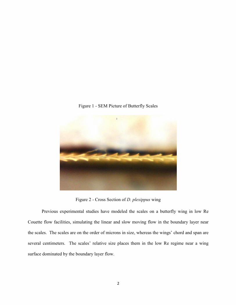
Figure 1
Figure
Previous experimental studies have modeled the scales on a butterfly wing in
Couette flow facilities, simulating the linear and slow moving flow in the boundary layer near
the scales. The scales are on the order of microns
several centimeters. The scales’ relative size places them
surface dominated by the boundary layer flow.
2
Figure 1 - SEM Picture of Butterfly Scales
Figure 2 - Cross Section of D. plexippus wing
Previous experimental studies have modeled the scales on a butterfly wing in
low facilities, simulating the linear and slow moving flow in the boundary layer near
on the order of microns in size, whereas the wings’ chord
The scales’ relative size places them in the low Re regime near a wing
surface dominated by the boundary layer flow.
Previous experimental studies have modeled the scales on a butterfly wing in low Re
low facilities, simulating the linear and slow moving flow in the boundary layer near
chord and span are
in the low Re regime near a wing

3
1.2 Objectives
The ultimate objectives of this and similar studies are to understand the aerodynamic
effects of embedded cavity geometries on a butterfly's wing and to determine any potential
applications to micro-air vehicles. The specific objectives of the following research are to
construct a computational model capable of qualitatively modeling the flow field near and inside
embedded cavities inside of a steady Couette flow to determine if the cavities can reduce the
shear drag on the moving plate relative to a Couette flow. First, the computational models will
recreate the rectangular and parallelogram cavity models used in Jones (2011) and Johnson
(2009).
4
2. BACKGROUND
2.1 Theory
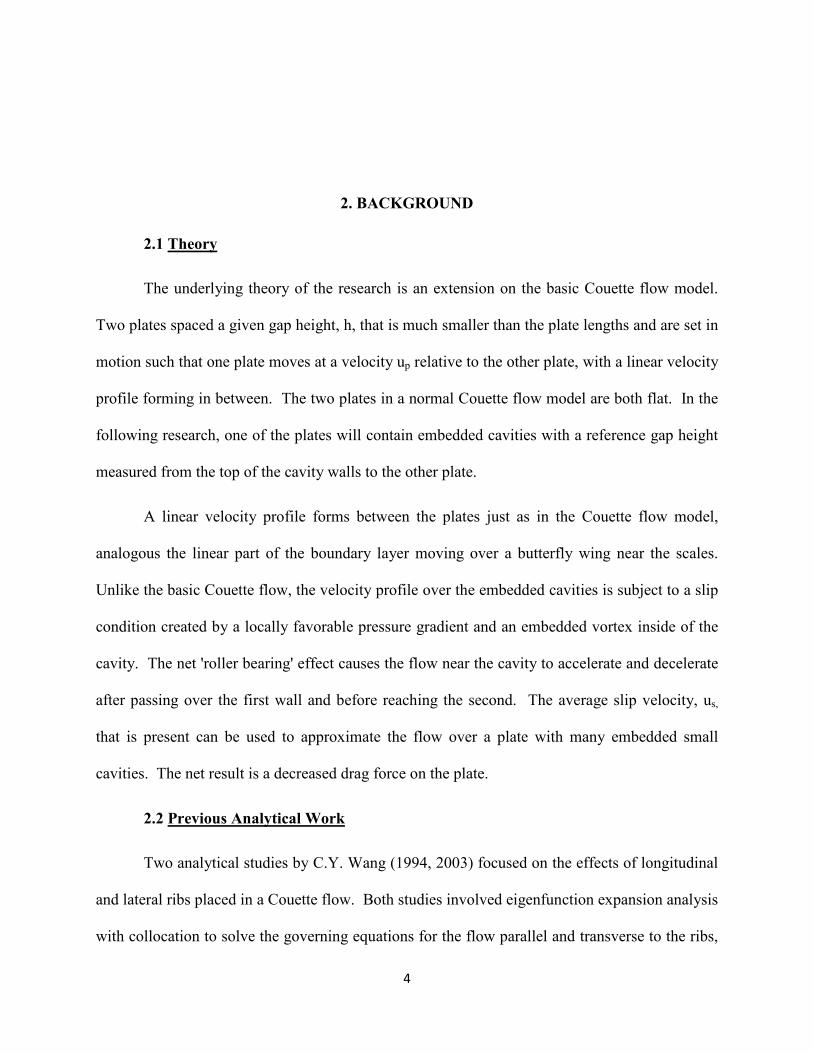
The underlying theory of the research is an extension on the basic Couette flow model.
Two plates spaced a given gap height, h, that is much smaller than the plate lengths and are set in
motion such that one plate moves at a velocity up relative to the other plate, with a linear velocity
profile forming in between. The two plates in a normal Couette flow model are both flat. In the
following research, one of the plates will contain embedded cavities with a reference gap height
measured from the top of the cavity walls to the other plate.
A linear velocity profile forms between the plates just as in the Couette flow model,
analogous the linear part of the boundary layer moving over a butterfly wing near the scales.
Unlike the basic Couette flow, the velocity profile over the embedded cavities is subject to a slip
condition created by a locally favorable pressure gradient and an embedded vortex inside of the
cavity. The net 'roller bearing' effect causes the flow near the cavity to accelerate and decelerate
after passing over the first wall and before reaching the second. The average slip velocity, us,
that is present can be used to approximate the flow over a plate with many embedded small
cavities. The net result is a decreased drag force on the plate.
2.2 Previous Analytical Work
Two analytical studies by C.Y. Wang (1994, 2003) focused on the effects of longitudinal
and lateral ribs placed in a Couette flow. Both studies involved eigenfunction expansion analysis
with collocation to solve the governing equations for the flow parallel and transverse to the ribs,
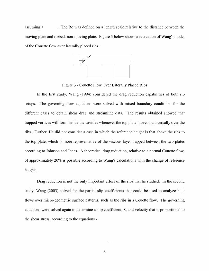
assuming a . The Re was defined on a length scale relative to the distance between the
moving plate and ribbed, non-moving plate.
of the Couette flow over laterally placed ribs.
Figure 3 -
In the first study, Wang
setups. The governing flow equations
different cases to obtain shear drag and streamline data
trapped vortices will form inside the cavities whenever the top plate moves transversally over the
ribs. Further, He did not consider a case in which the reference height is that above the ribs to
the top plate, which is more representative of the viscous layer trapped between the two plates
according to Johnson and Jones.
of approximately 20% is possible according to Wang's calculations with the change of
heights.
Drag reduction is not the only important effect of the ribs that
study, Wang (2003) solved for the partial slip coefficients that could be used to analyze bulk
flows over micro-geometric surface patterns, s
equations were solved again to determine a slip coefficient
the shear stress, according to the equation
5
. The Re was defined on a length scale relative to the distance between the
moving plate. Figure 3 below shows a recreation of Wang's model
of the Couette flow over laterally placed ribs.
Couette Flow Over Laterally Placed Ribs
, Wang (1994) considered the drag reduction capabilities of both rib
governing flow equations were solved with mixed boundary conditions
different cases to obtain shear drag and streamline data. The results obtained showed that
trapped vortices will form inside the cavities whenever the top plate moves transversally over the
He did not consider a case in which the reference height is that above the ribs to
s more representative of the viscous layer trapped between the two plates
. A theoretical drag reduction, relative to a normal Couette flow
of approximately 20% is possible according to Wang's calculations with the change of
is not the only important effect of the ribs that he studied.
solved for the partial slip coefficients that could be used to analyze bulk
geometric surface patterns, such as the ribs in a Couette flow.
equations were solved again to determine a slip coefficient, S, and velocity that is proportional to
the shear stress, according to the equations -
. The Re was defined on a length scale relative to the distance between the
below shows a recreation of Wang's model
considered the drag reduction capabilities of both rib
solved with mixed boundary conditions for the
. The results obtained showed that
trapped vortices will form inside the cavities whenever the top plate moves transversally over the
He did not consider a case in which the reference height is that above the ribs to
s more representative of the viscous layer trapped between the two plates
relative to a normal Couette flow,
of approximately 20% is possible according to Wang's calculations with the change of reference
studied. In the second
solved for the partial slip coefficients that could be used to analyze bulk
uch as the ribs in a Couette flow. The governing
and velocity that is proportional to
6
The results obtained in Wang (2003) showed that the drag reduction is proportional to the
slip coefficient over the cavity. The slip coefficient varied with the geometry and placement of
the cavities. The result means an optimum cavity configuration may exist that maximizes the
slip coefficient, thereby potentially maximizing the drag reduction capabilities at the Stokes
limit.
In addition to Wang's analytical studies, Scholle (2007) used an analytical approach with
Fourier analysis to determine the effects of roughness on shear forces between two parallel
plates. His model uses cavities that are sinusoidal in shape, rather than the rectangular
considered by Wang (1994, 2003). Scholle (2007) determined that if the plates were within a
distance of each other on the same length scale as the cavity amplitudes, there was potential for
drag reduction of up to 10% for their flow regime. The amount of drag reduction was based on
the distance between the plates and the cavity geometry.
2.3 Previous Computational Work
In addition to analytical studies, similar computational research has been conducted on
the use of embedded cavities. At NASA, Gatski and Grosch (1985) created a computational
model that considered an actual boundary layer flow, rather than a Couette flow, over an
embedded cavity as shown in Figure 4 below. The cavity's size was based on a length scale
referenced by the height of the laminar boundary layer over a flat plate at the position of the
cavity.

Figure 4 - Boundary Layer Flow Over a Single Embedded Cavity
The results obtained by Gatski and Grosch's computational model found that a single
embedded cavity provides a negligible contribution in terms o
over a flat plate in the cavity vicinity.
pressure gradient are also present inside the cavity. Gatski and Grosch
despite the lack of any noticeable drag reduction with one cavity, the presence of multiple
cavities optimally sized and spaced
an adverse pressure gradient forms.
Savoie and Gagnon (1995)
over embedded cavities. They constructed a cavity whose structure was more triangular, as
shown in Figure 5, and used a vorticity
equations for flow over the cavity. Just as with Gatski and Grosch
unbounded. A periodic boundary condition is imposed on either side of the triangular cavity, the
cavity itself is a wall where the no
free stream.
Their results showed that for very low Reynolds numbers, i.e. Re < 100, a vortex forms
inside of the cavity and stays within the cavity, creating a recirculation region. The study cited
by Savoi and Gagnon (1995) was limited
considered.
7
Boundary Layer Flow Over a Single Embedded Cavity
The results obtained by Gatski and Grosch's computational model found that a single
provides a negligible contribution in terms of drag reduction relative to the drag
over a flat plate in the cavity vicinity. However, an embedded vortex and a net favorable
resent inside the cavity. Gatski and Grosch (1985)
despite the lack of any noticeable drag reduction with one cavity, the presence of multiple
optimally sized and spaced could reduce drag and delay boundary layer separation when
an adverse pressure gradient forms.
(1995) have also used computational methods to simulate the flow
over embedded cavities. They constructed a cavity whose structure was more triangular, as
, and used a vorticity-stream function method to solve the Navier Stokes
ow over the cavity. Just as with Gatski and Grosch (1985)
unbounded. A periodic boundary condition is imposed on either side of the triangular cavity, the
cavity itself is a wall where the no-slip condition is applied, and the top boundary
Their results showed that for very low Reynolds numbers, i.e. Re < 100, a vortex forms
inside of the cavity and stays within the cavity, creating a recirculation region. The study cited
was limited to flow visualization and no drag reduction results were
Boundary Layer Flow Over a Single Embedded Cavity
The results obtained by Gatski and Grosch's computational model found that a single
f drag reduction relative to the drag
However, an embedded vortex and a net favorable
(1985) postulated that
despite the lack of any noticeable drag reduction with one cavity, the presence of multiple
could reduce drag and delay boundary layer separation when
have also used computational methods to simulate the flow
over embedded cavities. They constructed a cavity whose structure was more triangular, as
stream function method to solve the Navier Stokes
(1985), their flow is
unbounded. A periodic boundary condition is imposed on either side of the triangular cavity, the
slip condition is applied, and the top boundary condition is a
Their results showed that for very low Reynolds numbers, i.e. Re < 100, a vortex forms
inside of the cavity and stays within the cavity, creating a recirculation region. The study cited
to flow visualization and no drag reduction results were
8
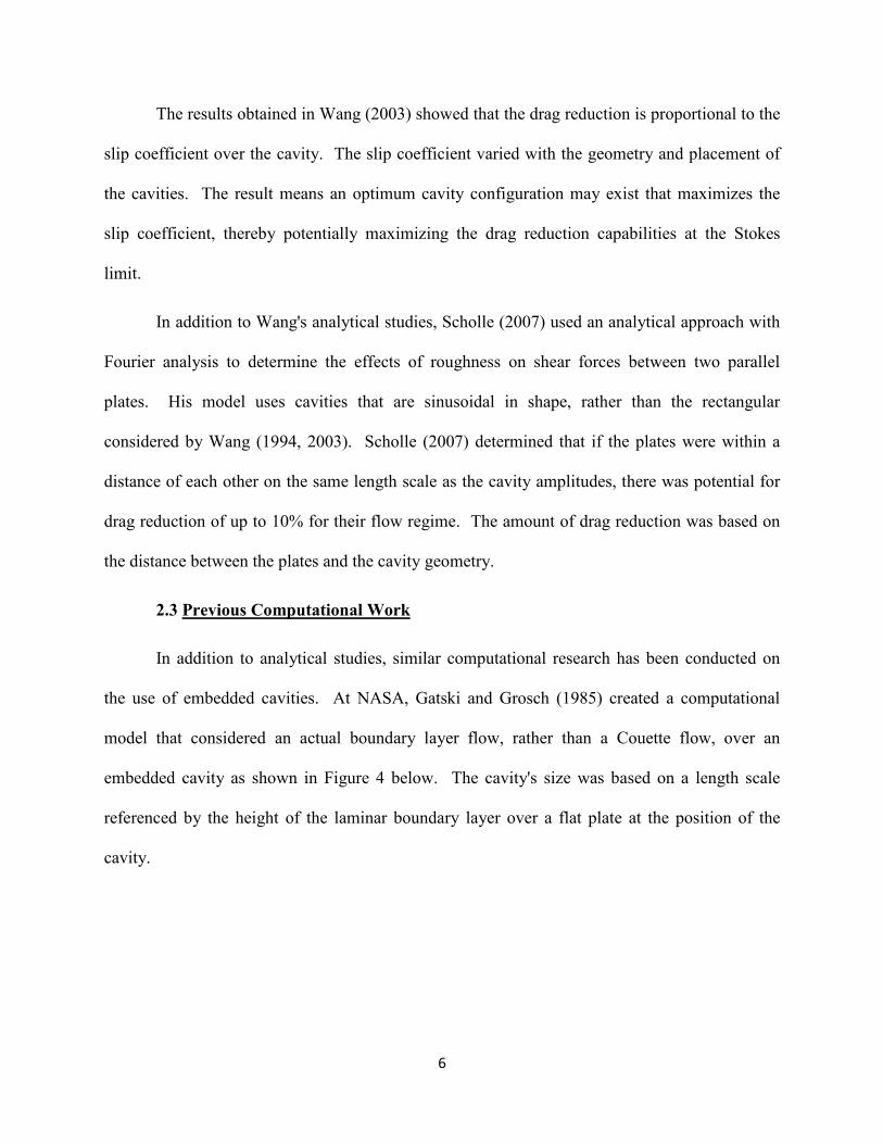
Scholle et al (2006) also showed the presence of a ‘roller bearing effect’ inside of a
sinusoidal shaped cavity that stemmed from the presence of an embedded vortex. The effect was
a partial slip velocity along the top of the cavity where there was rotating fluid, rather than a flat
surface.
Figure 5 - Triangular Cavity Model
2.4 Previous Experimental Work
The analytical and computational studies considered have made predictions about the
effects of embedded cavity geometries in boundary layer and Couette flows. The predictions
must be validated by experimental studies, such as the studies conducted by Taneda (1979),
Bechert et al. (1989), Johnson (2009), and Jones (2011). The four studies consider an embedded
cavity geometry and attempt to experimentally verify the flow mechanism postulated from
earlier analytical studies and biological observation.
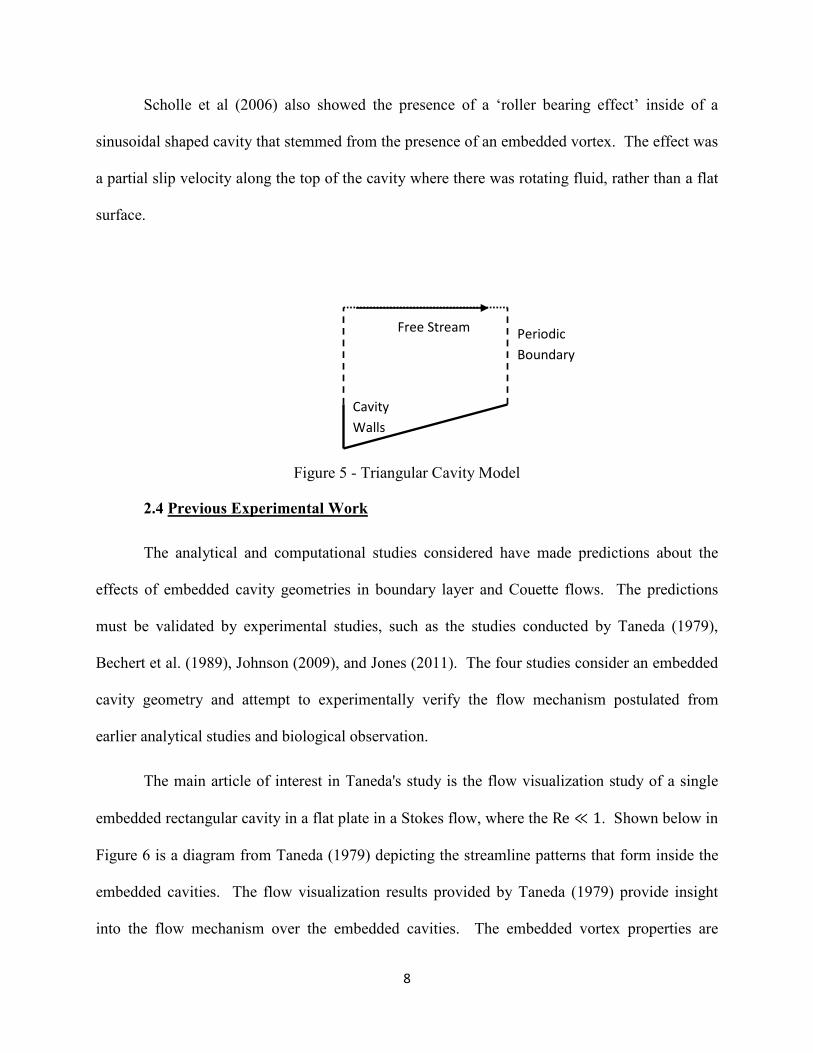
The main article of interest in Taneda's study is the flow visualization study of a single
embedded rectangular cavity in a flat plate in a Stokes flow, where the � � �. Shown below in
Figure 6 is a diagram from Taneda (1979) depicting the streamline patterns that form inside the
embedded cavities. The flow visualization results provided by Taneda (1979) provide insight
into the flow mechanism over the embedded cavities. The embedded vortex properties are
Free Stream Periodic Boundary
Cavity Walls
shown to vary with the cavity geometry.
results for comparison with the computational models
any quantitative flow data on drag reduction or the pressure and shear force distribut
Figure 6 - Streamline Patterns Over an
The experimental results obtained by Bechert et al.
(2011) provide quantitative data that can be used to analyze the effects of the embedded cavity
geometries. Johnson and Jones' analys
et al. and will be discussed further.
plate with embedded cavity geometries inside of a low Re Couette Flow facility. The drag forces
measured on the plate with the embedded geometries are compared to similar results obtained in
the facility for a flat plate simulati
The results obtained shown below in
reduce the drag in a Couette flow, but that the reduction is a function of the cavity geometry and
Re. In particular the drag reduction reduces to less than five percent
9
the cavity geometry. Further, the flow visualization provides
for comparison with the computational models. However, Taneda's study did not provide
flow data on drag reduction or the pressure and shear force distribut
Streamline Patterns Over an Embedded Cavities at Re = 0.01
The experimental results obtained by Bechert et al. (1989), Johnson (2009)
provide quantitative data that can be used to analyze the effects of the embedded cavity
' analyses are partially based on the work performed by Bechert
and will be discussed further. Johnson's experiment involved placing an experimental flat
plate with embedded cavity geometries inside of a low Re Couette Flow facility. The drag forces
measured on the plate with the embedded geometries are compared to similar results obtained in
the facility for a flat plate simulating a Couette Flow.
The results obtained shown below in Figure 7 show that the embedded cavities can
reduce the drag in a Couette flow, but that the reduction is a function of the cavity geometry and
In particular the drag reduction reduces to less than five percent starting approximately at
Further, the flow visualization provides qualitative
. However, Taneda's study did not provide
flow data on drag reduction or the pressure and shear force distributions.
Embedded Cavities at Re = 0.01
(2009), and Jones
provide quantitative data that can be used to analyze the effects of the embedded cavity
partially based on the work performed by Bechert
cing an experimental flat
plate with embedded cavity geometries inside of a low Re Couette Flow facility. The drag forces
measured on the plate with the embedded geometries are compared to similar results obtained in
show that the embedded cavities can
reduce the drag in a Couette flow, but that the reduction is a function of the cavity geometry and
starting approximately at a

10
Re of 25 and continues diminishing as Re is further increased. Jones’ work expanded on
Johnson’s by measuring the drag reduction capabilities of additional embedded cavity models, in
particular geometries that resembled the cavity geometry in between scales on a butterfly. These
geometries involved parallelogram, rather than rectangular, cavities that had inclined walls.
Figure 7 - Drag Reduction v. Re Plot I
Figure 8 - Drag Reduction v. Re Plot II
-1
-0.8
-0.6
-0.4
-0.2
0
0.2
0.4
0.6
0 10 20 30 40 50 60 70 80
η
Re
Cavity Model, Forward
Cavity Model, Reverse
Finned Model
11
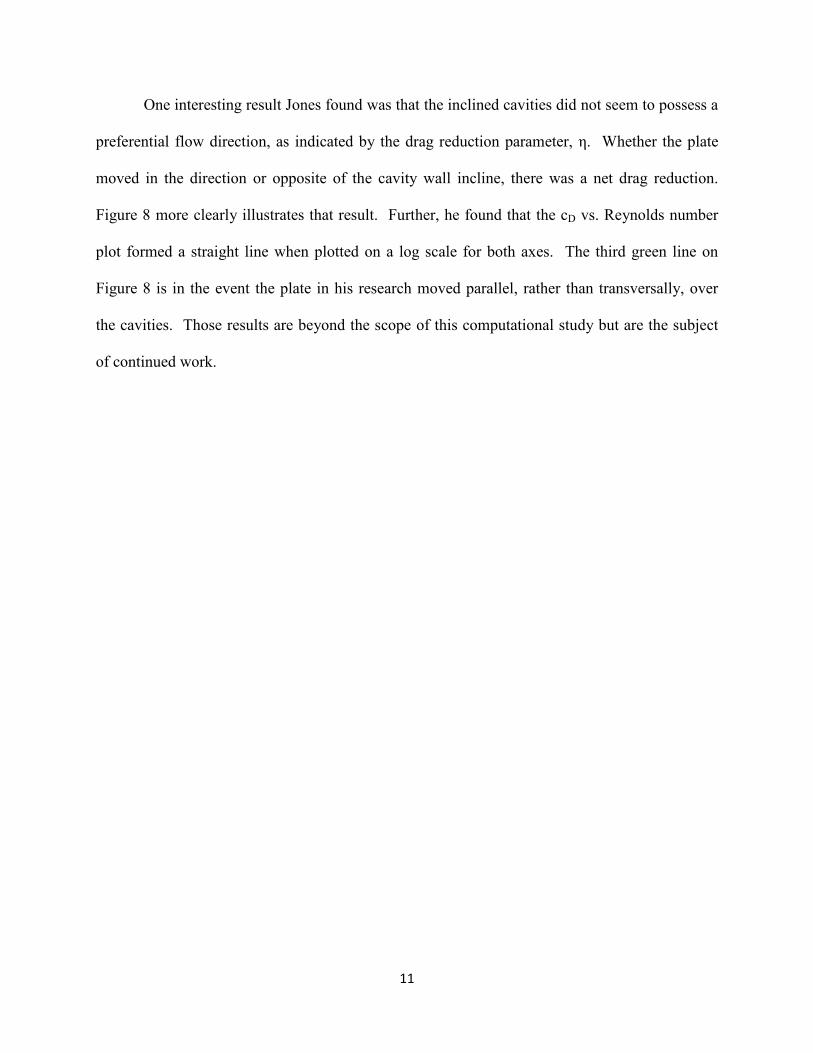
One interesting result Jones found was that the inclined cavities did not seem to possess a
preferential flow direction, as indicated by the drag reduction parameter, η. Whether the plate
moved in the direction or opposite of the cavity wall incline, there was a net drag reduction.
Figure 8 more clearly illustrates that result. Further, he found that the cD vs. Reynolds number
plot formed a straight line when plotted on a log scale for both axes. The third green line on
Figure 8 is in the event the plate in his research moved parallel, rather than transversally, over
the cavities. Those results are beyond the scope of this computational study but are the subject
of continued work.
12
3. COMPUTATIONAL PROCEDURE
3.1 Problem Setup
The model used in the following research was constructed and analyzed using ANSYS 13
and the computational fluid dynamics (CFD) code FLUENT. CFD’s flexibility provided a time
efficient alternative to experiments that provide limited data, especially in regards to flow
visualization. The CFD model was validated qualitatively by previous experimental results from
Johnson and Jones.
3.2 Computational Model
The computational model was created by considering the section of a plate over a single
cavity, as shown below in Figure 9. The cavity was setup with a desired AR and then the top
plate was spaced the desired distance of h above the cavity for the desired β. The top plate and
cavity walls were set as wall boundary conditions where the no-slip condition applies. The
remaining edges were made into periodic boundary conditions, simulating a plate with infinitely
many embedded cavities. The top wall moved at a given up that induced a linear velocity profile,
U(y), at the cavity's inlet edge. The fluid inside the model was set at zero initial velocity with no
externally applied pressure gradient. The flow Re was primarily controlled by varying up and h.
� � ����� �

Figure 9
3.3 Computational Procedure
The computational model
modeler and meshing programs
model such that what would otherwise be a continuous system described by the Navier
equations can be a discrete system solved at a finite amount of points. The output slowly
converges to the actual solution to the problem as the mesh is refined and more nodes are used.
However, the amount of computing time is also increased. After a grid refinement analysis, the
results between subsequent tests had a negligible percent difference for a me
nodes per unit length. See section 4.1 for more details on the grid refinement
After constructing a suitable mesh, it was imported into FLUENT
setup the proper initial flow conditions mentioned in section 3.2
solution. The uniform placement of nodes
arising from poorly shaped fluid elements.
plate moving at a constant velocity
based solver was used instead.
simulations. The convergence criteria for FLUENT's residuals was set at 10
13
Figure 9 - Computational Model
Computational Procedure
The computational model constructed and meshed using the ANSYS 13 geometry
modeler and meshing programs. The mesh consists of various nodes placed throughout the
model such that what would otherwise be a continuous system described by the Navier
equations can be a discrete system solved at a finite amount of points. The output slowly
he actual solution to the problem as the mesh is refined and more nodes are used.
However, the amount of computing time is also increased. After a grid refinement analysis, the
results between subsequent tests had a negligible percent difference for a mesh consisting of
See section 4.1 for more details on the grid refinement.
After constructing a suitable mesh, it was imported into FLUENT. FLUENT was used to
setup the proper initial flow conditions mentioned in section 3.2 and numerically obtain a
The uniform placement of nodes was for simplicity and to prevent numerical
arising from poorly shaped fluid elements. A time-dependent solution was unnecessary
plate moving at a constant velocity because of the laminar flow at low Re. A
Specifically, a SIMPLE power law algorithm was used for all
The convergence criteria for FLUENT's residuals was set at 10
constructed and meshed using the ANSYS 13 geometry
. The mesh consists of various nodes placed throughout the
model such that what would otherwise be a continuous system described by the Navier-Stokes
equations can be a discrete system solved at a finite amount of points. The output slowly
he actual solution to the problem as the mesh is refined and more nodes are used.
However, the amount of computing time is also increased. After a grid refinement analysis, the
sh consisting of 30
FLUENT was used to
numerically obtain a
was for simplicity and to prevent numerical errors
dependent solution was unnecessary for a
steady, pressure
Specifically, a SIMPLE power law algorithm was used for all
The convergence criteria for FLUENT's residuals was set at 10-6. FLUENT
14
calculates its residuals via the following formula, where � could be a component of velocity or
some other scalar value:
���� �������� � �
The primary models analyzed were based on experimental work by Taneda, Johnson, and
Jones and on the observed butterfly cavity geometries. The flows were also analyzed over a
range of Re. Specifically:
AR = 1, φ = 90°, β = 2, 1, � , �!
AR = 2, φ = 45°, β = 1 AR = 3, φ = 26°, β = 1
Re: 0.01, 0.1, 1, 5, 10, 15, 20, 25, 30, 40, 50, 60, 70, 75, 80, 90, 100
The pertinent data gathered for each simulation included streamline contours, dividing streamline
height, slip velocity distribution, and shear and pressure drag on the cavities.

15
4. RESULTS AND DISCUSSION
4.1 Grid Refinement
The primary goal of the research is to determine any possible reductions in drag on the
bottom plate with the cavities versus a Couette flow without the cavities. By Newton's Second
Law, the total sum of pressure and shear forces on the cavity have to balance out the pressure
and shear forces on the moving plate above the cavity for equilibrium. The grid refinement
study uses that fact by comparing the distribution of shear and pressure forces in the x-direction
for different meshes. The remaining results are analyzed using the second most refined mesh,
whose results differ minimally from the most refined, to minimize computation time.
The study was conducted on the AR 1 square cavity with a β of one. All meshes used in
the research were uniform. For the grid refinement study the meshes used had 10, 20, 30, and
finally 40 nodes per unit length. Figure 10 below is a picture of the meshes used.

16
Figure 10 - 1x1 Cavity Meshes

17
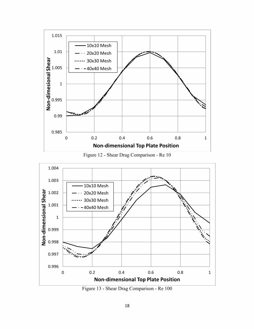
The Reynolds number range tested in the research was between 0.01 and 100. Only Re =
1, 10, and 100 were considered for the grid refinement study. The results of the shear drag on
the top plate are below in Figures 11 - 13. Notice that the results 30 nodes per length and 40
nodes per length meshes lie almost on top of each other. The main differences between the two
meshes lie at the left and right edges of the plate. The results are close enough however that the
remaining results of the research shown in the next sections used 30 nodes per unit length along
the edges of the cavities and the top plate for the AR 1 square cavity.
Figure 11 - Shear Drag Comparison - Re 1
0.985
0.99
0.995
1
1.005
1.01
1.015
0 0.2 0.4 0.6 0.8 1
Non
-dim
ensi
onal
She
ar
Non-dimensional Top Plate Position
10x10 Mesh
20x20 Mesh
30x30 Mesh
40x40 Mesh
18
Figure 12 - Shear Drag Comparison - Re 10
Figure 13 - Shear Drag Comparison - Re 100
0.985
0.99
0.995
1
1.005
1.01
1.015
0 0.2 0.4 0.6 0.8 1
Non
-dim
esio
nal S
hear
Non-dimensional Top Plate Position
10x10 Mesh
20x20 Mesh
30x30 Mesh
40x40 Mesh
0.996
0.997
0.998
0.999
1
1.001
1.002
1.003
1.004
0 0.2 0.4 0.6 0.8 1
Non
-dim
ensi
onal
She
ar
Non-dimensional Top Plate Position
10x10 Mesh
20x20 Mesh
30x30 Mesh
40x40 Mesh

19
The AR 2 cavity with a 45 degree incline used 45 nodes along the inclined walls and
triangle shaped elements in the cavity domain to improve the accuracy. The AR 3 cavity with a
26 degree incline used closer to 40 nodes per unit length along the inclined and bottom cavity
walls and on the top plate. The primary reason is because of the skew in the triangular elements
used in the cavity domain. The inclination of the cavity is severe enough that proper node
spacing, especially for a uniform mesh, is paramount to ensure that the triangular elements are
adequately shaped. If the elements are too skewed, the flow simulations may never converge on
a solution and/or any solutions that do converge may not be accurate. Pictures of the meshes
used for the remaining results are shown below in Figure 14.
Figure 14 - Embedded Cavity Meshes

20
4.2 Flow Visualization
(a) (b)
(c) (d)
Figure 15 - AR 1 Cavity Streamlines at Re = (a) 1 (b) 10 (c) 50 (d) 100

21
(a) (b)
(c) (d)
Figure 16 - AR 2 Cavity Streamlines at Re = (a) 1 (b) 10 (c) 50 (d) 100
22
(a) (b)
(c) (d)
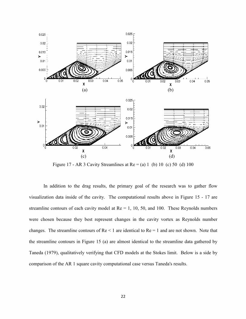
Figure 17 - AR 3 Cavity Streamlines at Re = (a) 1 (b) 10 (c) 50 (d) 100
In addition to the drag results, the primary goal of the research was to gather flow
visualization data inside of the cavity. The computational results above in Figure 15 - 17 are
streamline contours of each cavity model at Re = 1, 10, 50, and 100. These Reynolds numbers
were chosen because they best represent changes in the cavity vortex as Reynolds number
changes. The streamline contours of Re < 1 are identical to Re = 1 and are not shown. Note that
the streamline contours in Figure 15 (a) are almost identical to the streamline data gathered by
Taneda (1979), qualitatively verifying that CFD models at the Stokes limit. Below is a side by
comparison of the AR 1 square cavity computational case versus Taneda's results.
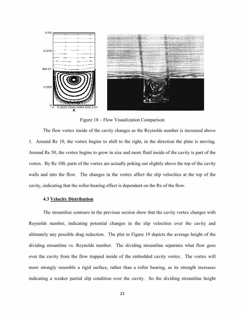
Figure 1
The flow vortex inside of the cavity changes as the Reynolds number is increased above
1. Around Re 10, the vortex begins to shift to the right,
Around Re 50, the vortex begins to grow in size and more fluid inside of the cavity is part of the
vortex. By Re 100, parts of the vortex are actually poking out slightly above the top of the cavity
walls and into the flow. The changes in the vortex
cavity, indicating that the roller-bearing effect is dependent on the Re of the flow.
4.3 Velocity Distribution
The streamline contours in the previous section show that the c
Reynolds number, indicating potential changes in the slip velocities over the cavity and
ultimately any possible drag reduction. The plot in
dividing streamline vs. Reynolds number. Th
over the cavity from the flow trapped inside of the embedded cavity vortex. The vortex will
more strongly resemble a rigid surface, rather than a roller bearing, as its strength increases
indicating a weaker partial slip condition over the cavity. So the dividing streamline height
23
Figure 18 – Flow Visualization Comparison
The flow vortex inside of the cavity changes as the Reynolds number is increased above
1. Around Re 10, the vortex begins to shift to the right, in the direction the plate is moving.
Around Re 50, the vortex begins to grow in size and more fluid inside of the cavity is part of the
vortex. By Re 100, parts of the vortex are actually poking out slightly above the top of the cavity
he changes in the vortex affect the slip velocities at the top of the
bearing effect is dependent on the Re of the flow.
Velocity Distribution
The streamline contours in the previous section show that the cavity vortex changes with
Reynolds number, indicating potential changes in the slip velocities over the cavity and
ultimately any possible drag reduction. The plot in Figure 19 depicts the average height of the
dividing streamline vs. Reynolds number. The dividing streamline separates what flow goes
over the cavity from the flow trapped inside of the embedded cavity vortex. The vortex will
more strongly resemble a rigid surface, rather than a roller bearing, as its strength increases
partial slip condition over the cavity. So the dividing streamline height
The flow vortex inside of the cavity changes as the Reynolds number is increased above
in the direction the plate is moving.
Around Re 50, the vortex begins to grow in size and more fluid inside of the cavity is part of the
vortex. By Re 100, parts of the vortex are actually poking out slightly above the top of the cavity
affect the slip velocities at the top of the
bearing effect is dependent on the Re of the flow.
avity vortex changes with
Reynolds number, indicating potential changes in the slip velocities over the cavity and
depicts the average height of the
e dividing streamline separates what flow goes
over the cavity from the flow trapped inside of the embedded cavity vortex. The vortex will
more strongly resemble a rigid surface, rather than a roller bearing, as its strength increases
partial slip condition over the cavity. So the dividing streamline height

24
needs to be high enough such that the roller bearing effect is present, but low enough such that
the cavity provides optimal drag reduction.
Figure 19 - Average Dividing Streamline Height vs. Reynolds Number
Figure 20 - Slip Velocity Distribution Geometry Comparison I, β 1 Cavity
0.7
0.75
0.8
0.85
0.9
0.95
1
0 20 40 60 80 100Ave
rage
Non
-dim
ensi
onal
Div
idin
g St
ream
line
Hei
ght
Reynolds Number
AR 1, Beta 1
AR 1, Beta 2
AR 2, Beta 1, 45 Deg
AR 3, Beta 1, 26 Deg
0
0.05
0.1
0.15
0.2
0.25
0 0.2 0.4 0.6 0.8 1
Non
-dim
ensi
onal
Vel
ocit
y
Non-dimensional Cavity Position
AR 1, 90 Deg, Re 0.01
AR 2, 45 Deg, Re 0.01
AR 3, 26 Deg, Re 0.01
25
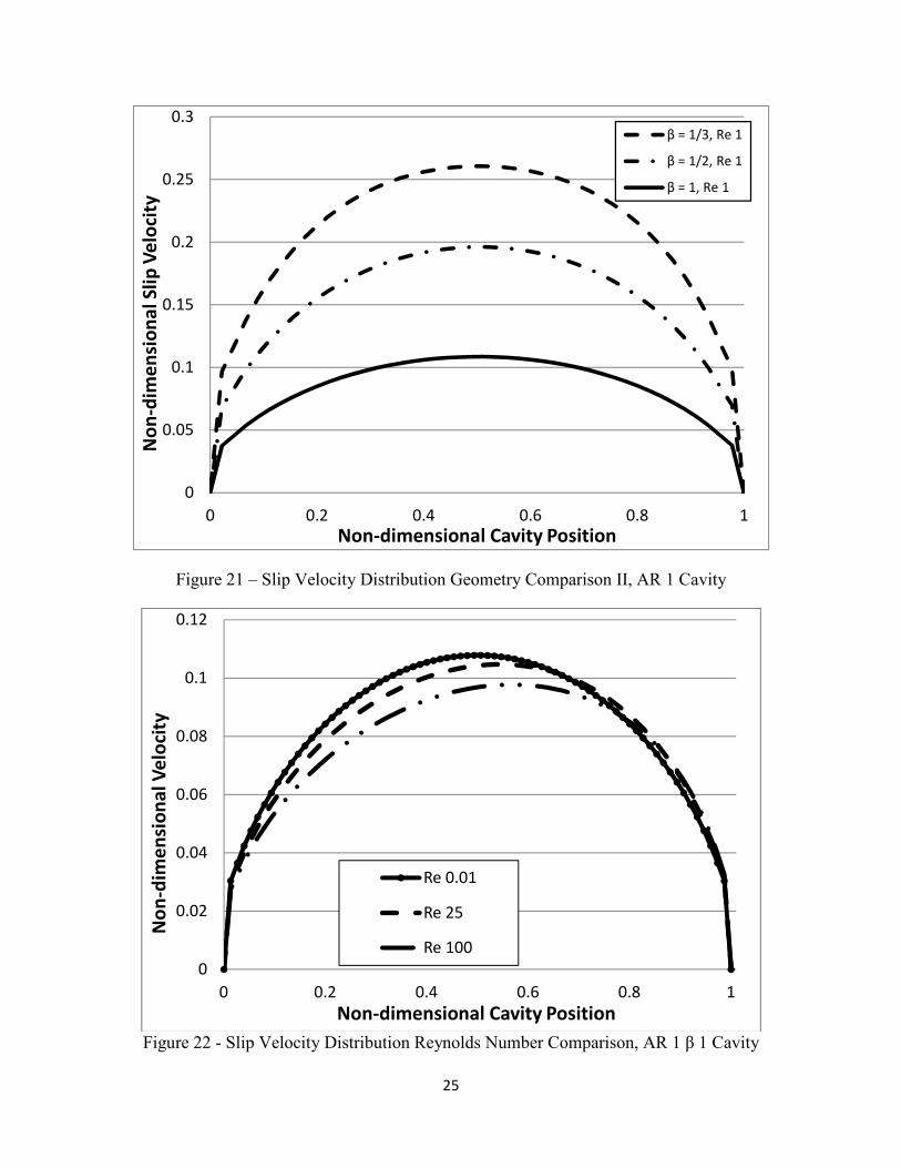
Figure 21 – Slip Velocity Distribution Geometry Comparison II, AR 1 Cavity
Figure 22 - Slip Velocity Distribution Reynolds Number Comparison, AR 1 β 1 Cavity
0
0.05
0.1
0.15
0.2
0.25
0.3
0 0.2 0.4 0.6 0.8 1
Non
-dim
ensi
onal
Slip
Vel
ocit
y
Non-dimensional Cavity Position
β = 1/3, Re 1
β = 1/2, Re 1
β = 1, Re 1
0
0.02
0.04
0.06
0.08
0.1
0.12
0 0.2 0.4 0.6 0.8 1
Non
-dim
ensi
onal
Vel
ocit
y
Non-dimensional Cavity Position
Re 0.01
Re 25
Re 100

26
Figure 23 - Average Slip Velocity vs. Reynolds Number
The plots in Figure 20 - 23 are various plots of the slip velocity distribution over the
cavity. The 'slip velocity' is the horizontal velocity present at the top of the cavities, where a
plate would usually be in a Couette flow. According to Wang, the us is proportional to the drag
reduction.
Figure 20 shows the slip velocity distribution at Re = 0.01 for each geometry. Note that
the higher aspect ratio cavities have much higher peaks in comparison to the AR 1 cavity. They
are also slightly asymmetric, which is to be expected given their inclination. Figure 21 compares
the effect of β on the slip velocities for the AR cavity. Decreasing the value of β has a similar
effect as increasing aspect ratio for the values shown. However, these results are limited to a
finite range of AR and β. As the former gets high enough, the flow will dip into the cavity and
potentially separate. If the latter is small enough, the solution for shear stress more closely
0.06
0.08
0.1
0.12
0.14
0.16
0.18
0 10 20 30 40 50 60 70 80 90 100
Non
-dim
ensi
onal
Ave
rage
Slip
Vel
ocit
y
Reynolds Number
AR=1
AR=2, 45 Deg Inc
AR=3, 26 Deg Inc
27
resembles that for a lid driven cavity. If β is big enough, the effects of the cavities become
negligible on the global flow field.
Figure 22 shows the slip velocity distribution for the AR 1, β 1 cavity at different
Reynolds numbers. As Re increases, the slip velocity distribution becomes more asymmetric
and the maximum value is also lower. The slip velocity distributions for the other cavities
follow the same pattern. Figure 23 is a plot of the us for each cavity vs. Re at β =1.
Based on Figures 21 - 23, the higher AR and lower β cavities have higher drag reduction
potential than the AR 1 cavity at low Re. Further, the drag reduction is highest at the Stokes
limit and decreases from there as Re increases.
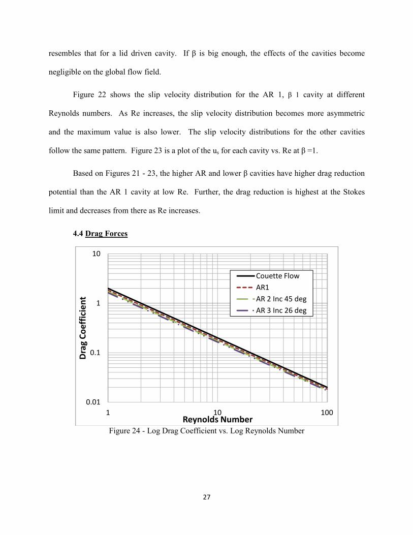
4.4 Drag Forces
Figure 24 - Log Drag Coefficient vs. Log Reynolds Number
0.01
0.1
1
10
1 10 100
Dra
g Co
effic
ient
Reynolds Number
Couette FlowAR1AR 2 Inc 45 degAR 3 Inc 26 deg
28
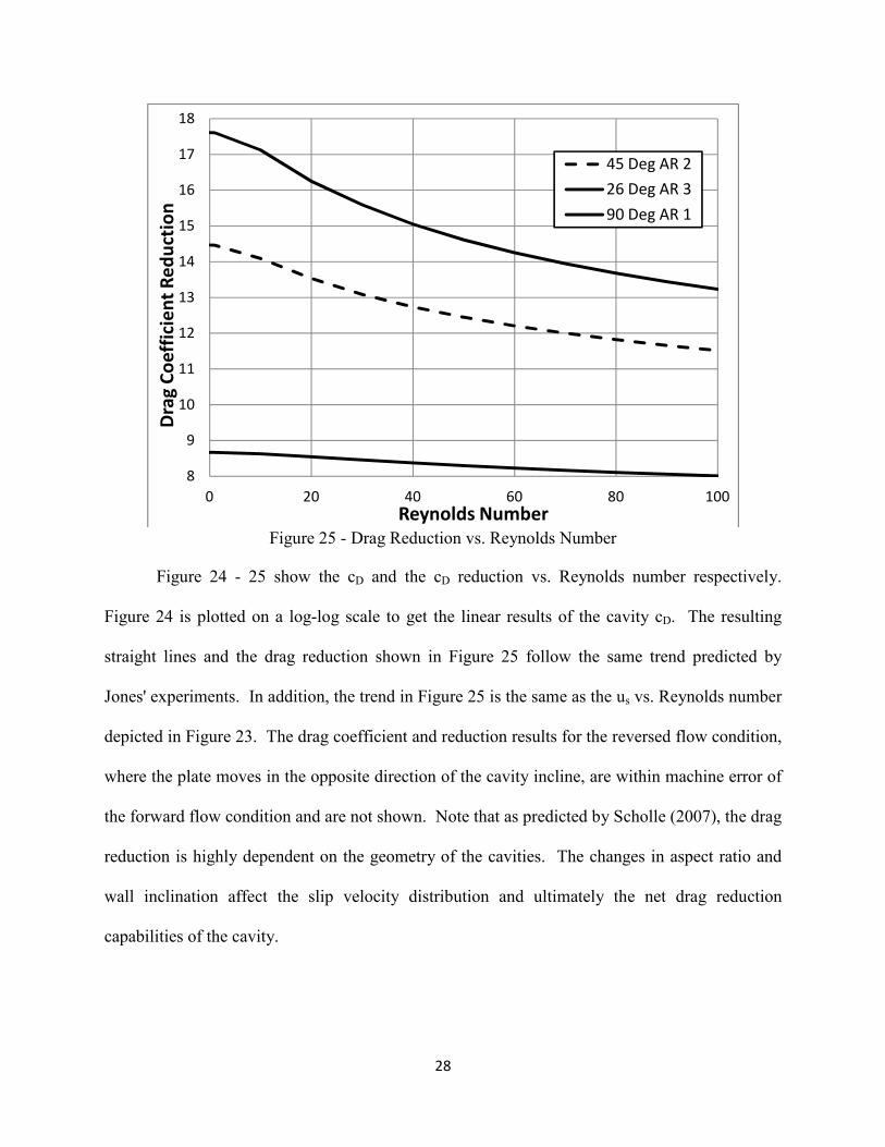
Figure 25 - Drag Reduction vs. Reynolds Number
Figure 24 - 25 show the cD and the cD reduction vs. Reynolds number respectively.
Figure 24 is plotted on a log-log scale to get the linear results of the cavity cD. The resulting
straight lines and the drag reduction shown in Figure 25 follow the same trend predicted by
Jones' experiments. In addition, the trend in Figure 25 is the same as the us vs. Reynolds number
depicted in Figure 23. The drag coefficient and reduction results for the reversed flow condition,
where the plate moves in the opposite direction of the cavity incline, are within machine error of
the forward flow condition and are not shown. Note that as predicted by Scholle (2007), the drag
reduction is highly dependent on the geometry of the cavities. The changes in aspect ratio and
wall inclination affect the slip velocity distribution and ultimately the net drag reduction
capabilities of the cavity.
8
9
10
11
12
13
14
15
16
17
18
0 20 40 60 80 100
Dra
g Co
effic
ient
Red
ucti
on
Reynolds Number
45 Deg AR 2
26 Deg AR 3
90 Deg AR 1
29
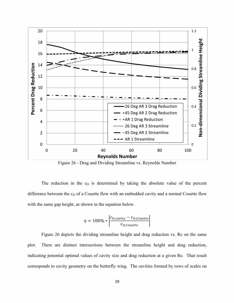
Figure 26 - Drag and Dividing Streamline vs. Reynolds Number
The reduction in the cD is determined by taking the absolute value of the percent
difference between the cD of a Couette flow with an embedded cavity and a normal Couette flow
with the same gap height, as shown in the equation below.
" � �##$ % &'()*+,-./ 0 '()1234..4'()1234..4 & Figure 26 depicts the dividing streamline height and drag reduction vs. Re on the same
plot. There are distinct intersections between the streamline height and drag reduction,
indicating potential optimal values of cavity size and drag reduction at a given Re. That result
corresponds to cavity geometry on the butterfly wing. The cavities formed by rows of scales on
0
0.2
0.4
0.6
0.8
1
1.2
0
2
4
6
8
10
12
14
16
18
20
0 20 40 60 80 100
Non
-dim
ensi
onal
Div
idin
g St
ream
line
Hei
ght
Perc
ent D
rag
Redu
ctio
n
Reynolds Number
26 Deg AR 3 Drag Reduction45 Deg AR 2 Drag ReductionAR 1 Drag Reduction26 Deg AR 3 Streamline45 Deg AR 2 StreamlineAR 1 Streamline
30
a butterfly wing are not uniformly sized. Near the center of the wing, the cavities are around AR
2 to 3. However, the cavities shrink to lower AR towards the trailing edge of the wing.
4.5 Computational vs. Experimental Results
The qualitative computational results obtained thus far match experimental predictions
made by Johnson (2009) and Jones (2011). Further, the AR 1 streamline contours match the
flow visualization images obtained in Taneda's experiments. The embedded cavity contributes to
a net drag reduction via a roller-bearing effect from an embedded vortex that form a partial slip
condition over the cavity. The partial slip condition is reduced at higher Re which manifests as a
reduced drag reduction capability from the presence of the cavity inside of the flow. Further, the
CFD models predict that there is not a preferential flow direction.
While the data follows all of the above trends, the actual values of the drag reduction are
approximately half of what Jones' experiments predicted, as shown in Figure 27. Experimental
data was only collected up to Re of about 75, whereas the computational data goes to an Re of
100. The quantitative data shows that the computational model predicts a lower drag reduction
capability than experimentally determined. There are a few possible reasons for the
disagreement.

31
Figure 27 - Computational versus Experimental Results
The first two are numerical in nature. The tips of the walls of the cavity form a
discontinuity in terms of flow velocity with the mesh. The velocity at the wall is zero while just
above the velocity is in the form of some linear profile from the moving top plate and to the right
is the cavity. The ANSYS model considers the cavity walls to be infinitely thin. The actual
scales on a butterfly wing are thin, but not infinitely thin in comparison to the length scale of the
cavities formed on the butterfly wing. The same is true for the cavity walls in Jones'
experimental models. A possible solution that will be tried in future studies is to give the walls
some characteristic width and check if the drag reduction results obtained are a closer match to
experimental predictions.
In addition to the cavity wall tip discontinuity, there is a singularity formed at the corner
of the cavity as determined in Wang's second study. According to Wang (2003), the singularity
0
10
20
30
40
50
60
0 10 20 30 40 50 60 70 80 90 100
Perc
ent R
educ
tion
Ove
r Ca
viti
es
Reynolds Number
Experimental, Cavity 26 Deg AR 3
Experimental, Cavity 45 Deg AR 2
Computational, 26 Deg AR 3
Computational, 45 Deg AR 2

32
formed at the corner could contribute to numerical inaccuracies, especially if a node is placed in
the corner. For analytical studies, Wang (2003) suggested subtracting out the analytical form of
the singularity before running simulations. Given that the preceding results were obtained with
FLUENT, the only other solution is grid refinement and careful node placement in the
neighborhood of the cavity.
The remaining possible reason for disagreement in the computational and experimental
results is based on the experimental calculation of drag reduction by Jones (2011). The
experimental models consisted of a plate that had a region with the cavities and a region that was
flat. A force was measured over that plate and compared to a plate of the same size that did not
possess the cavities. The percent difference in the forces on the plates was considered to be the
same as the difference in the drag. Unfortunately, that assumes the entire flat region around the
cavity region is a perfect Couette flow solution. Given the disparity in the shear distribution for
Couette flow and the cavities, it is plausible that there is a region AROUND the cavities in the
plate that has a shear distribution in between that of the cavities and a Couette flow. If so, that
region would have a higher average drag than the cavity region and lower than a Couette flow.
The result would be a higher drag reduction prediction than is actually present.

33
5. CONCLUSIONS
5.1 Computational Model and Results
The computational model of the Couette flow with embedded cavities is an imperfect
guide for the experimental research of embedded cavity geometries. The cavities are able to
reduce the shear drag in a Couette flow via an embedded vortex inside of the cavity that imposes
a slip condition, versus a no-slip condition, where the bottom wall in a Couette flow would
normally be. Increased aspect ratio and reduced gap height lead to better drag reduction
potential at low Reynolds numbers. Regardless of geometry, the drag reduction potential of the
embedded cavities reduces with Reynolds number, correlating with a reduced average slip
velocity distribution versus Reynolds number. The computational data follows the qualitative,
but not quantitative, trends of the experimental results.
Despite the lack of a quantitative match to experimental expectations, the model does
match predictions from the other analytical and computational studies and can serve as a
qualitative guide to future experiments that determine slip velocities near the cavity, flow
visualization, drag reduction, and/or other data trends.
Future studies should also consider a further important note. The gap height to cavity
ratio, β, was kept constant because the top plate was fixed. The flow was bounded in this regard.
The periodic boundary conditions and fixed height of the plate made it appear as though a flat
plate were moving over a large amount of cavities at a fixed height. In an unbounded flow

34
scenario, where there is a boundary layer that forms over a surface with the cavities, the height of
the boundary layer will not be the same.
Even on a flat surface, a boundary layer’s height is a function of Reynolds number and
position on the surface. If cavities are added to this surface, the boundary layer formation
mechanism could change. It may no longer be self-similar, the height and growth rate of the
boundary layer could change, and other effects regarding separation, vortex formation, or
transition to turbulence could all be affected. Changes in the height of the boundary layer
present an interesting problem based on the results of this research.
The fixed position of the flat plate in the following studies mimicked the height of the
linear region of the boundary layer, above which is the non-linear region. In an unbounded flow
scenario, the height of the boundary layer will grow. In the simulations performed, an increase
in that height corresponds to an increased β. The trend in the computational results showed that
potential drag reduction is reduced as β increases.
5.2 Ongoing Work
The computational models presented here are only for three different geometries.
Ongoing work by the author includes determining the effects of geometric changes in aspect
ratio, inclination angle, and gap to cavity height versus Reynolds number in more detail. The
results could be useful not only for future embedded cavity studies for aerodynamic applications,
but also for other applications involving thin films or shear dominated flows such as those
considered by Mickaily (1992) and Ryu (1986).
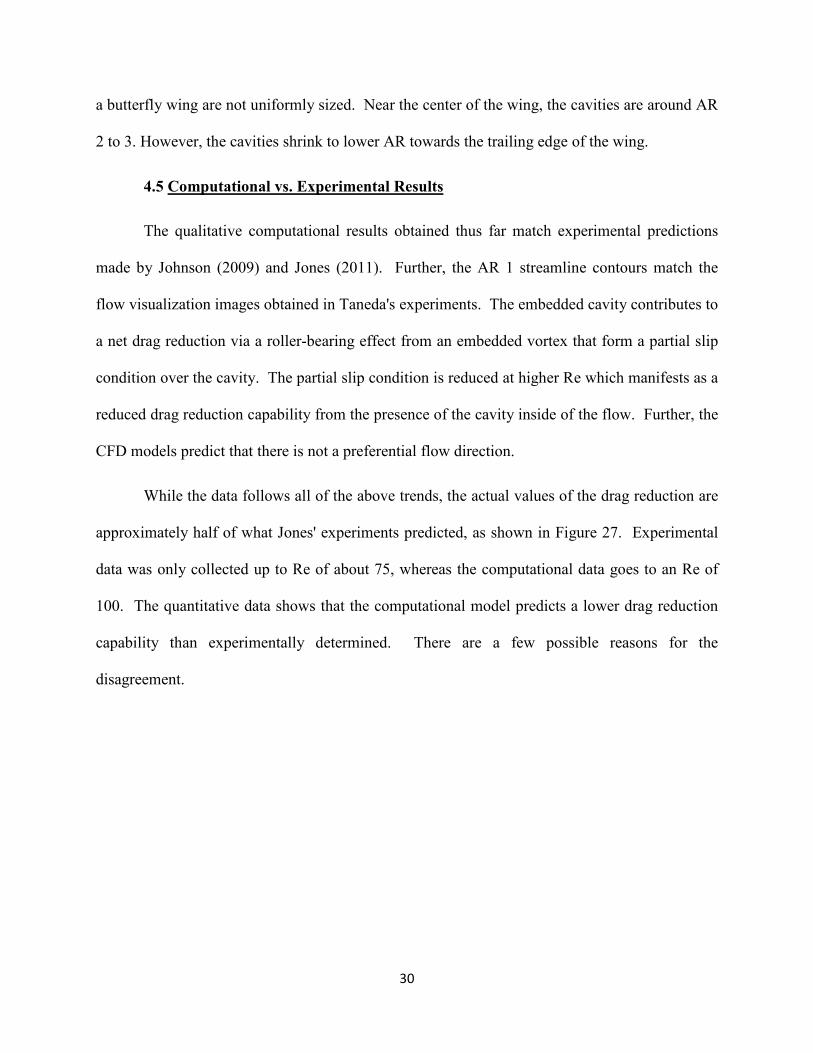
In addition to the changes in cavity geometry, there is ongoing work to create a three-
dimensional model of the cavities. The models shown in this research and proposed above for
further study are only two-dimensional. In reality, the flow is more complicated and consists of
longitudinal and transverse flows through and over the cavities. A three
pictured in Figure 28 consists of a top plate moving at a constant velocity within a two
dimensional plane over successive rows of cavities. The new model will be able to
simultaneously simulate the longitudinal and transverse flow fields.
Figure 28 - Thr
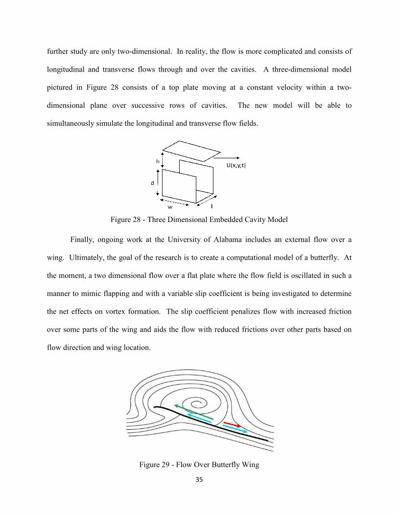
Finally, ongoing work at the University of Alabama includes an external flow over a
wing. Ultimately, the goal of the research is to create a computational model of a butterfly. At
the moment, a two dimensional flow over a
manner to mimic flapping and with a variable slip coefficient is being investigated to determine
the net effects on vortex formation.
over some parts of the wing and aids
flow direction and wing location.
Figure 29
35
dimensional. In reality, the flow is more complicated and consists of
longitudinal and transverse flows through and over the cavities. A three-dimensional model
consists of a top plate moving at a constant velocity within a two
dimensional plane over successive rows of cavities. The new model will be able to
simultaneously simulate the longitudinal and transverse flow fields.
Three Dimensional Embedded Cavity Model
Finally, ongoing work at the University of Alabama includes an external flow over a
wing. Ultimately, the goal of the research is to create a computational model of a butterfly. At
the moment, a two dimensional flow over a flat plate where the flow field is oscillated in such a
manner to mimic flapping and with a variable slip coefficient is being investigated to determine
the net effects on vortex formation. The slip coefficient penalizes flow with increased friction
over some parts of the wing and aids the flow with reduced frictions over other parts based on
flow direction and wing location.
Figure 29 - Flow Over Butterfly Wing
dimensional. In reality, the flow is more complicated and consists of
dimensional model
consists of a top plate moving at a constant velocity within a two-
dimensional plane over successive rows of cavities. The new model will be able to
Finally, ongoing work at the University of Alabama includes an external flow over a
wing. Ultimately, the goal of the research is to create a computational model of a butterfly. At
is oscillated in such a
manner to mimic flapping and with a variable slip coefficient is being investigated to determine
The slip coefficient penalizes flow with increased friction
the flow with reduced frictions over other parts based on

36
5.3 Future Work
The computational model created for the current research works as a qualitative guide to
the actual boundary layer flow that forms near the surface of a butterfly's wings. The following
research and ongoing work consists of parallelogram shaped cavities. The scales on a Monarch
butterfly wing possess slight curvature in addition to being inclined as shown below in Figure 30.
Further, the scales are not infinitely thin in comparison to the size of the cavity. Future studies
should consider the effects of the cavity curvature and thickness on the flow.
Figure 30 - 400x Magnification Monarch Butterfly Wing Cross-section
The embedded cavity models can only provide qualitative data trends on the complex
flow over a butterfly wing. A more accurate model based on the computational study performed
by Gatski and Grosch (1985) could provide further insight. The new model would simulate
multiple embedded cavities in a boundary layer flow as shown below in Figure 31. According to
Gatski and Grosch (1985), the net effect of several optimally spaced and sized cavities could
delay boundary layer separation and reduce the drag over an airfoil. A more accurate partial slip
condition could also be obtained from such a model and then applied to an external flow model
over a wing. Further, more accurate data can be obtained for sizing the cavities on a physical
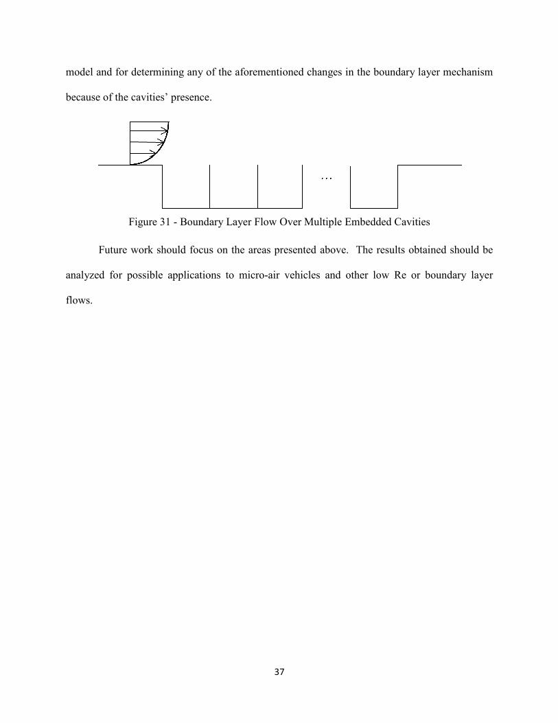
model and for determining any of the aforementioned changes in the boundary layer mechanism
because of the cavities’ presence.
Figure 31 - Boundary Layer Flow Over Multiple Embedded Cavities
Future work should focus
analyzed for possible applications to micro
flows.
37
model and for determining any of the aforementioned changes in the boundary layer mechanism
because of the cavities’ presence.
Boundary Layer Flow Over Multiple Embedded Cavities
Future work should focus on the areas presented above. The results obtained should be
for possible applications to micro-air vehicles and other low Re or boundary layer
model and for determining any of the aforementioned changes in the boundary layer mechanism
Boundary Layer Flow Over Multiple Embedded Cavities
. The results obtained should be
or boundary layer
38
6. BIBILIOGRAPHY
Bechert, D.W., Bartenwerfer, M., and Hoppe, G., “Turbulent Drag Reduction on Non-planar Surfaces”, IUTAM Symposium on Structure of Turbulence and Drag Reduction, Zurich, Switzerland, 1989 Chebbi, B., and Tavoularis, S., “Low Reynolds Number Flow In and Above Asymmetric, Triangular Cavities”, Physics of Fluids A, 2, pp. 1044-1046, June 1990 Gatski, T.B., and Grosch, C.E., “Embedded Cavity Drag in Steady Laminar Flow”, AIAA 22nd Aerospace Sciences Meeting, Reno, NV, pp. 1028-1037, Jan. 1984 Johnson, Tyler J., “Drag Measurements Across Patterned Surfaces in a Low Reynolds Number Couette Flow Facility”, Master’s Thesis, The University of Alabama, 2009 Jones, Robert A., “Drag Measurements Over Embedded Cavities Inspired by the Microgeometry Formed by Butterfly Scales”, Master’s Thesis, The University of Alabama, 2011 Leibenguth, Chase, Lang, Amy, and Schreiber, Will, "Computational Analysis of Low Reynolds Number Couette Flow Over an Embedded Cavity Geometry", 64th American Physical Society Division of Fluid Dynamics Conference, Baltimore, MD, Nov. 2011 Leibenguth, Chase, Lang, Amy, and Schreiber, Will, "Computational Analysis of Low Reynolds Number Couette Flow Over Embedded Cavities", 63rd American Physical Society Division of Fluid Dynamics Conference, Long Beach, CA, Nov. 2010 Martin, Michael J., and Boyd, Iain D., “Blasius Boundary Layer Solution with Slip Flow Conditions”, 22nd International Symposium on Rarefied Gas Dynamics, Sydney, Australia, pp. 518-523, July 2000 Matthews, Miccal T., and Hill, James M., “A note on the boundary equations with linear slip boundary condition”, Applied Mathematics Letters, vol. 21, issue 8, pp. 810-813, September 2007 Mickaily, Elizabeth S., Middelman, Stanley, and Allen, Merry, “Viscous Flow Over Periodic Surfaces”, Chemical Engineering Communications, vol. 117, pp. 401-414, May 1992 Palmore, John and Sharif, M.A.R., "CFD Analysis of Flow Over a Flat Plate with Gradient Based Slip Condition", 64thAmerican Physical Society Division of Fluid Dynamics Conference, Baltimore, MD, Nov. 2011 Philip, John R., “Flows Satisfying Mixed No-Slip and No-Shear Conditions”, Journal of Applied Mathematics and Physics, vol. 23, pp. 353-372, Feb. 1972
39
Ryu, Hwa Won and Chang, Ho Nam, "Creeping Flows in Rectangular Cavities with Translating Top and Bottom Walls: Numerical Study and Flow Visualization", Korean Journal of Chemical Engineering, vol. 3, no. 2, pp. 177-185, Sept. 1986 Savoie, Rodrigue and Gagnon, Yves, “Numerical Simulation of the Flow over a Model of the Cavities on a Butterfly Wing”, Journal of Thermal Science, vol. 4, no. 3, pp. 185-192, 1995 Schoelle, M. "Hydrodynamical Modeling of Lubricant Friction Between Rough Surfaces", Tribology International, vol. 40, pp. 1004-1011, 2007 Schoelle, M., Rund, A., & Askel N., “Drag reduction and improvement in material transport in creeping films”, Arch Apple Mech, vol. 75, pp. 93 – 113, 2006 Taneda, Sadatoshi, "Visualization of Separating Stokes Flows", Journal of the Physical Society of Japan, vol. 46, no. 6, pp. 1935-1942, June 1979 Wang, C.Y., “Flow Over a Surface with Parallel Grooves”, Physics of Fluids, vol. 15, no. 5, pp. 1114-1121, May 2003 Wang, C.Y., “The Stokes drag due to the sliding of a smooth plate over a finned plate”, Physics of Fluids, vol. 6, no. 7, pp. 2248-2252, Mar. 1994