Draft version submitted to J Hyd Eng Nov 2003 Evaluation of Numerical Models … HEC-RAS and DHI-MIKE 11

By William E. Fleenor1, Member, ASCE,and Mark R. Jensen 2

ABSTRACT: In “Evaluation of Numerical Models of Flood and Tide

Propagation” (ASCE Journal of Hydraulics Oct 2001), Rodney J. Sobey described six

benchmark tests for unsteady flow model validation. In this paper, two programs that

have been used extensively for flood stage prediction around the world, the Hydrologic

Engineering Center’s - River Analysis System (HEC- RAS) and the Danish Hydraulic

Institute’s (DHI) - MIKE 11 were applied to these benchmark tests. Both models

performed well on the benchmark tests. In addition to the theoretical benchmarks, this

paper also demonstrates that both models are capable of simulating observed transients in

the California Aqueduct.

INTRODUCTION:

In “Evaluation of Numerical Models of Flood and Tide Propagation” (Journal of Hydraulic

Engineering/October 2001), Sobey suggests that an “extensive and independent review … should be a

routine and automatic part of any numerical model study.” Sobey outlines six hydrodynamic tests for one-

dimensional, free surface numerical models, and provides sample output with his own ESTFLOW program.

The tests were designed to demonstrate the capabilities of the applied code and to expose any deficiencies

of the formulation or solution of the basic mass and momentum equations, equations (1) and (2)

respectively.

0=−∂∂

+∂∂ q

xQ

tb η (1)

px

gAA

Qxt

Q O

ρτη

−∂∂

−=

∂∂

+∂∂ 2

(2)

In this paper the ESTFLOW solutions are compared with the two models most commonly used in

flood stage prediction around the world, the public domain software of the Hydrologic Engineering

Center’s - River Analysis System (HEC-RAS) and the proprietary software of the Danish Hydraulic

1 Research Engineer, Civil & Environmental Engineering; 2001 EU III; UC Davis; One Shields Avenue;

Davis, CA 95616, wefleenor@ucdavis.edu, phone 530-752-5669, fax 530-752-7872 2 Ph.D. Candidate, Civil & Environmental Engineering; 2001 EU III, UC Davis; One Shields Avenue; UC

Davis; Davis, CA 95616 and Hydraulic Engineer, Hydrologic Engineering Center; 609 Second Street; Davis, CA 95616, mrjensen@ucdavis.edu, phone 530-756-1104, fax 530-752-7872

Draft version submitted to J Hyd Eng Nov 2003 Institute’s (DHI) - MIKE 11. Surprisingly, neither model has received peer-reviewed publication of its

efficacy in the past. In addition to the theoretical benchmarks, this paper also contains an application to the

San Joaquin Aqueduct in California where the transients were measured after an abrupt gate closing.

The models are introduced with a short discussion of the computational methodologies. In several of

the benchmark tests, Sobey presented the solutions as individual terms of the continuity and momentum

equations. The respective developers modified both HEC-RAS and MIKE 11 to output the terms of the

differential equations in order to provide a comparison with the benchmarks.

The ESTFLOW code used by Sobey to demonstrate his benchmark tests uses the method of

characteristics to solve the mass and momentum equation describing gradually varied, unsteady flow. The

method of characteristics uses a technique to change the underlying partial differential equations into a set

of ordinary differential equations that are solved using common Runge-Kutta solution techniques. The

exact formulation is detailed in Sobey’s paper.

General computational information common to HEC-RAS and MIKE 11

HEC-RAS and MIKE 11 are both general one dimensional (cross-section integrated) unsteady, open

channel, hydraulics programs. Both programs have modern graphical user interfaces with extensive plots

and tables to assist in setting up models and viewing output. They are capable of modeling natural cross

sections at irregular spacing (though all of Sobey’s benchmark tests use trapezoidal cross sections at regular

spacing). They have interfaces for commonly used GIS packages, which can be used to extract geometric

data from a terrain surface and delineate a floodplain from the computed water surfaces.

In preparation for unsteady computations, the programs compute tables of hydraulic properties, such

as flow area and top width as a function of water surface elevation. The tables are used to speed the

unsteady computations, see the sample cross section and table shown in Figure 1.

Figure 1. Sample cross section divided vertically for table of properties

Draft version submitted to J Hyd Eng Nov 2003 Internal boundaries, such as bridges and culverts, are preprocessed into a family of rating curves that

describe the head loss through a structure for a given tail water and flow. The hydraulics of internal

boundaries that change during the simulation, such as gated structures, are computed during the simulation.

HEC-RAS specific computational methodology information

The computation engine for the HEC-RAS program is based on the U.S. Army Corp of Engineer’s

(USACE) model Unsteady Network Model (UNET, Barkau, 1992). The program solves the mass

conservation and momentum conservation equations with an implicit linearized system of equations using

Preissman’s second order box scheme. In a cross section, the overbank and channel are assumed to have the

same water surface, though the overbank volume and conveyance are separate from the channel volume

and conveyance in the implementation of the conservation of mass and momentum equations. The

simultaneous system of equations generated for each time step (and iterations within a time step) are stored

with a skyline matrix scheme and reduced with a direct solver developed specifically for unsteady river

hydraulics by Dr. Robert Barkau.

The state variables for the numerical scheme are flow and stage, which are computed and stored at

each cross section. Plots of flow and stage are available for selected cross sections at a user specified time

interval.

The hydraulic resistance is based on the friction slope from the empirical Manning’s equation, with

several ways of modifying the roughness. Roughness can be characterized with Manning’s (n) or roughness

height’s (k).

DHI-MIKE 11 specific computational methodology information

The MIKE 11 solution of the continuity and momentum equations is based on an implicit finite

difference scheme developed by Abbott and Ionescu (1967). The scheme is setup to solve any form of the

Saint Venant equations – i.e. kinematic, diffusive, or dynamic. The water level and flow are calculated at

each time step, by solving the continuity equation and the momentum equation using a 6-point Abbot

scheme with the mass equation centered on h-points and the momentum equation centered on Q-points. By

default, the equations are solved with 2 iterations. The first iteration starts from the results of the previous

time step and the second uses the centered values from the first iteration. The number of iterations is user

specified.

Cross sections are easily specified in both area and longitudinal location through the user interface.

The water level (h points) is calculated at each cross section and at model interpolated interior points

located evenly and specified by the user-entered maximum distance. The flow (Q) is then calculated at

points midway between neighboring h-points and at structures.

The hydraulic resistance is based on the friction slope from the empirical equation, Manning’s or

Chezy, with several ways of modifying the roughness to account for variations throughout the cross-

sectional area.

Draft version submitted to J Hyd Eng Nov 2003 BENCHMARK TESTS

The benchmark tests are divided into three categories, modeling a single channel (C1-C3), modeling a

network (N1-N2), and modeling an inline hydraulic structure (S1). Each test has been designed so that the

stable solution has a Courant number less than one, providing conditions within the capabilities of a

practical numerical code. Please refer to Sobey’s original paper for a more detailed description of the

individual test cases.

Case C1: Steady, Uniform Flow in Open-Ended Channel

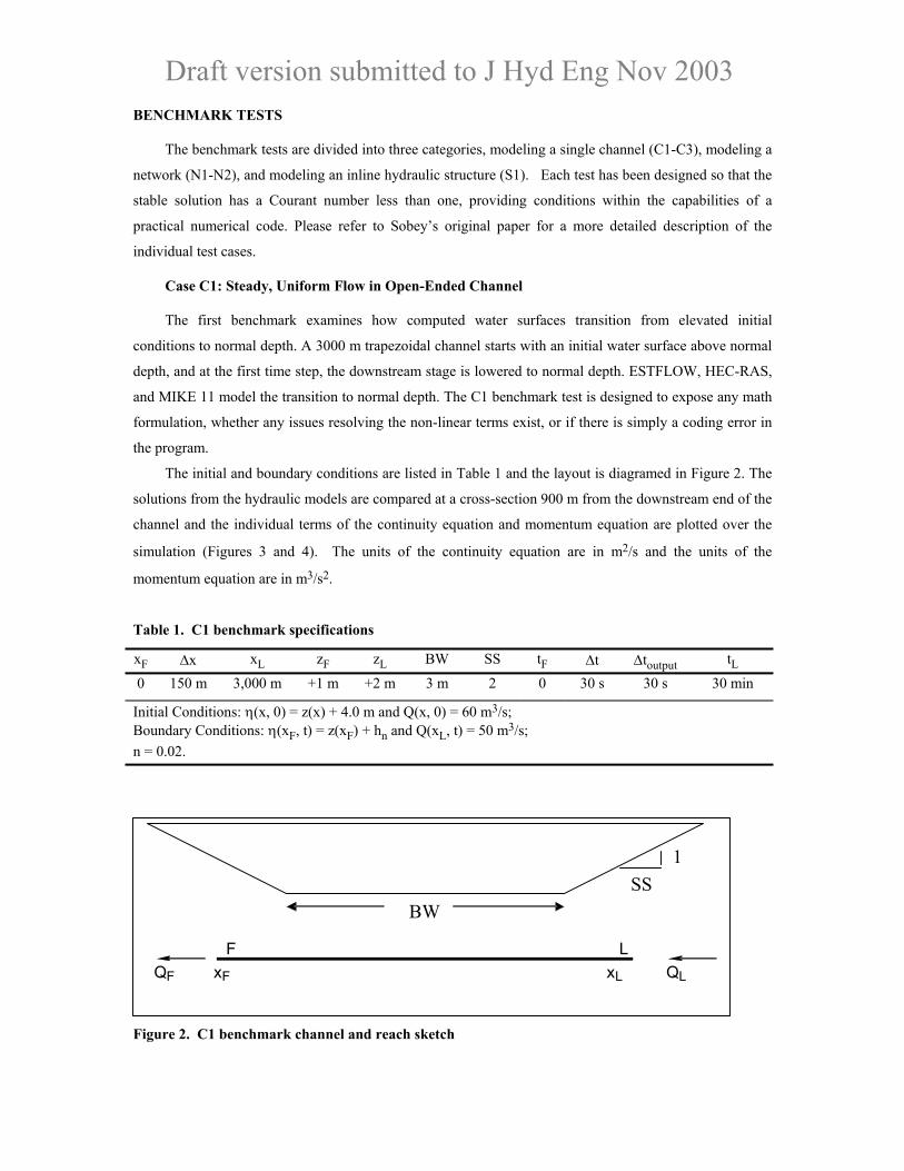
The first benchmark examines how computed water surfaces transition from elevated initial

conditions to normal depth. A 3000 m trapezoidal channel starts with an initial water surface above normal

depth, and at the first time step, the downstream stage is lowered to normal depth. ESTFLOW, HEC-RAS,

and MIKE 11 model the transition to normal depth. The C1 benchmark test is designed to expose any math

formulation, whether any issues resolving the non-linear terms exist, or if there is simply a coding error in

the program.

The initial and boundary conditions are listed in Table 1 and the layout is diagramed in Figure 2. The

solutions from the hydraulic models are compared at a cross-section 900 m from the downstream end of the

channel and the individual terms of the continuity equation and momentum equation are plotted over the

simulation (Figures 3 and 4). The units of the continuity equation are in m2/s and the units of the

momentum equation are in m3/s2.

Table 1. C1 benchmark specifications

xF ∆x xL zF zL BW SS tF ∆t ∆toutput tL

0 150 m 3,000 m +1 m +2 m 3 m 2 0 30 s 30 s 30 min

Initial Conditions: η(x, 0) = z(x) + 4.0 m and Q(x, 0) = 60 m3/s; Boundary Conditions: η(xF, t) = z(xF) + hn and Q(xL, t) = 50 m3/s; n = 0.02.

1 SS

BW

F L x F xL Q F Q L

Figure 2. C1 benchmark channel and reach sketch

Draft version submitted to J Hyd Eng Nov 2003

In descriptions of all benchmarks xF designates the longitudinal position of first cross section

(downstream), ∆x the space step, xL the longitudinal position of last cross section (upstream), zF the

downstream bed elevation, zL the downstream bed elevation, BW the bottom width, SS the side slopes

(horizontal to 1 vertical), tF the time at beginning of simulation, ∆t the computational time step, ∆toutput the

model output time step, tL the time at end of simulation, η(x, 0) the initial stage equation, z(x) the bed

elevation at x, Q(x, 0) the initial flow rate, η(xF, t) the downstream stage boundary condition, hn the normal

depth, Q(xL, t) the upstream flow boundary condition and n the Manning’s friction coefficient.

igure 3. C1 benchmark continuity equation terms

s noted in Sobey’s analysis, the 150 m cross-section spacing and a 30-second time step provide a

roug

F

A

h discretization of the problem. All models pass this difficult transient and go to normal depth while

preserving mass and momentum. If one desired to track this difficult drop in flow and stage, a smaller time

and space step would be required for these types of numerical schemes. Nothing unusual is demonstrated in

the graphs of the individual equation terms of the mass and momentum equations and all models show

reasonable conservation.

Draft version submitted to J Hyd Eng Nov 2003

Figure 4. C1 benchmark momentum equation terms

Case C2: Transient Evolution of Initial Mound

The second benchmark is a single reach that has a mound shaped profile for initial conditions that

spreads upstream and downstream during the unsteady simulation. The initial and boundary conditions for

this test are in Table 2. The numerical solutions, and a simplified analytical solution for this benchmark,

were compared with profiles at various times in the simulation (Figure 5). The simplified analytical

solution models the movement of a wave, but does not account for friction losses or boundary conditions.

Table 2. C2 benchmark specifications

xF ∆x xL zF zL BW SS tF ∆t ∆output tL 0 150 m 4,500 m +0 m +0 m 3 m 2 0 30 s 30 s 25 min

Initial Conditions: η(x, 0) = 2 + 0.2 exp{-c[(x – 2,250)/500]2} and Q(x, 0) = 0 m3/s; Boundary Conditions: Q(xF, t) = 0 m3/s and η(xL, t) = + 2 m; n = 0.02: c = log 2.

The mound from the initial conditions disperses in both directions and the numerical models follow

the simplified analytical solution for 360 seconds and then start to separate after the boundary conditions

start to impact the solution field (the analytical solution is not constrained by these boundary conditions).

The downstream boundary stage can change but the upstream stage is fixed. Both HEC-RAS and MIKE 11

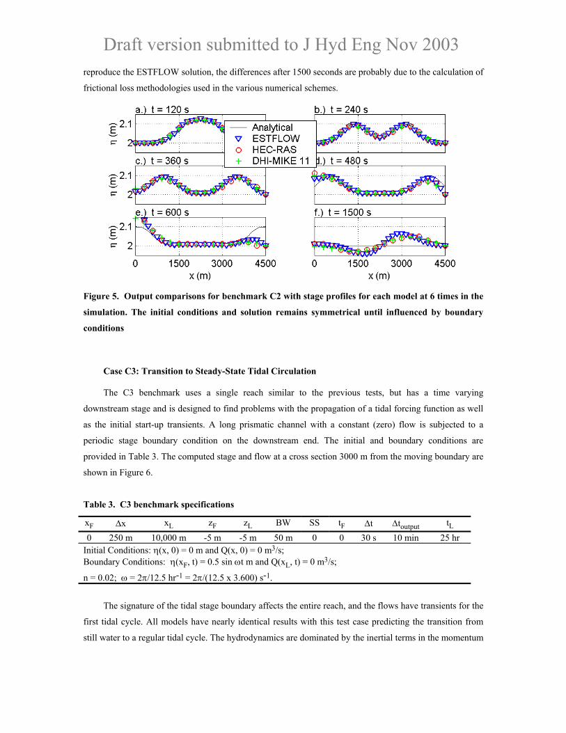
Draft version submitted to J Hyd Eng Nov 2003 reproduce the ESTFLOW solution, the differences after 1500 seconds are probably due to the calculation of

frictional loss methodologies used in the various numerical schemes.

Figure 5. Output comparisons for benchmark C2 with stage profiles for each model at 6 times in the

simulation. The initial conditions and solution remains symmetrical until influenced by boundary

conditions

Case C3: Transition to Steady-State Tidal Circulation

The C3 benchmark uses a single reach similar to the previous tests, but has a time varying

downstream stage and is designed to find problems with the propagation of a tidal forcing function as well

as the initial start-up transients. A long prismatic channel with a constant (zero) flow is subjected to a

periodic stage boundary condition on the downstream end. The initial and boundary conditions are

provided in Table 3. The computed stage and flow at a cross section 3000 m from the moving boundary are

shown in Figure 6.

Table 3. C3 benchmark specifications

xF ∆x xL zF zL BW SS tF ∆t ∆toutput tL 0 250 m 10,000 m -5 m -5 m 50 m 0 0 30 s 10 min 25 hr

Initial Conditions: η(x, 0) = 0 m and Q(x, 0) = 0 m3/s; Boundary Conditions: η(xF, t) = 0.5 sin ωt m and Q(xL, t) = 0 m3/s;

n = 0.02; ω = 2π/12.5 hr-1 = 2π/(12.5 x 3.600) s-1.

The signature of the tidal stage boundary affects the entire reach, and the flows have transients for the

first tidal cycle. All models have nearly identical results with this test case predicting the transition from

still water to a regular tidal cycle. The hydrodynamics are dominated by the inertial terms in the momentum

Draft version submitted to J Hyd Eng Nov 2003 balance; all three models utilize the same formulation for the inertial term and accordingly provide very

similar answers.

Figure 6. Output comparison for benchmark C3 at x = 3000 m

Case N1: Steady Flow through Channel Network

The N1 benchmark is the first network test case, and is diagramed in Figure 7. The test is analogous to

C1, in that the simulation is an examination of the transition to steady state from perturbed initial

conditions. The initial and boundary conditions are described in Table 4. The model solutions of the

computed stages at the internal junctions are compared in Figure 8 and the flow through the node “B”

confluence is compared in Figure 8.

Figure 7. Network Schematic for benchmarks N1 and N2

Table 4. N1 benchmark specifications

∆x tF ∆t ∆toutput tL 150 m 0 15 s 180 s 6 hr

Initial Conditions: η(x, 0) = +0.5 m and Q(x, 0) = 0 m3/s; Boundary Conditions: ηA( t) = 0 m and QD(t) = 100 m3/s and QE(t) = 50 m3/s; QD and QE introduced gradually by linear ramp function over 15 min.

Where ηA = stage at node A, QD= flow into node D, and QE = flow into node E.

Draft version submitted to J Hyd Eng Nov 2003

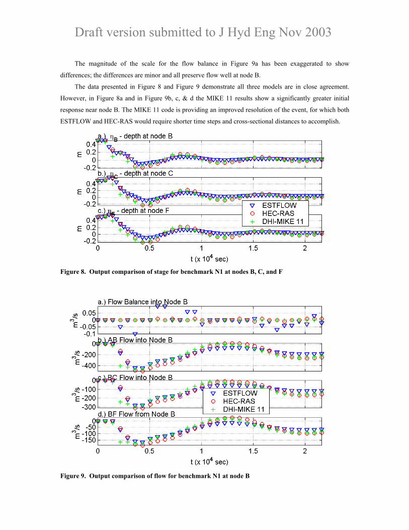
The magnitude of the scale for the flow balance in Figure 9a has been exaggerated to show

differences; the differences are minor and all preserve flow well at node B.

The data presented in Figure 8 and Figure 9 demonstrate all three models are in close agreement.

However, in Figure 8a and in Figure 9b, c, & d the MIKE 11 results show a significantly greater initial

response near node B. The MIKE 11 code is providing an improved resolution of the event, for which both

ESTFLOW and HEC-RAS would require shorter time steps and cross-sectional distances to accomplish.

Figure 8. Output comparison of stage for benchmark N1 at nodes B, C, and F

Figure 9. Output comparison of flow for benchmark N1 at node B

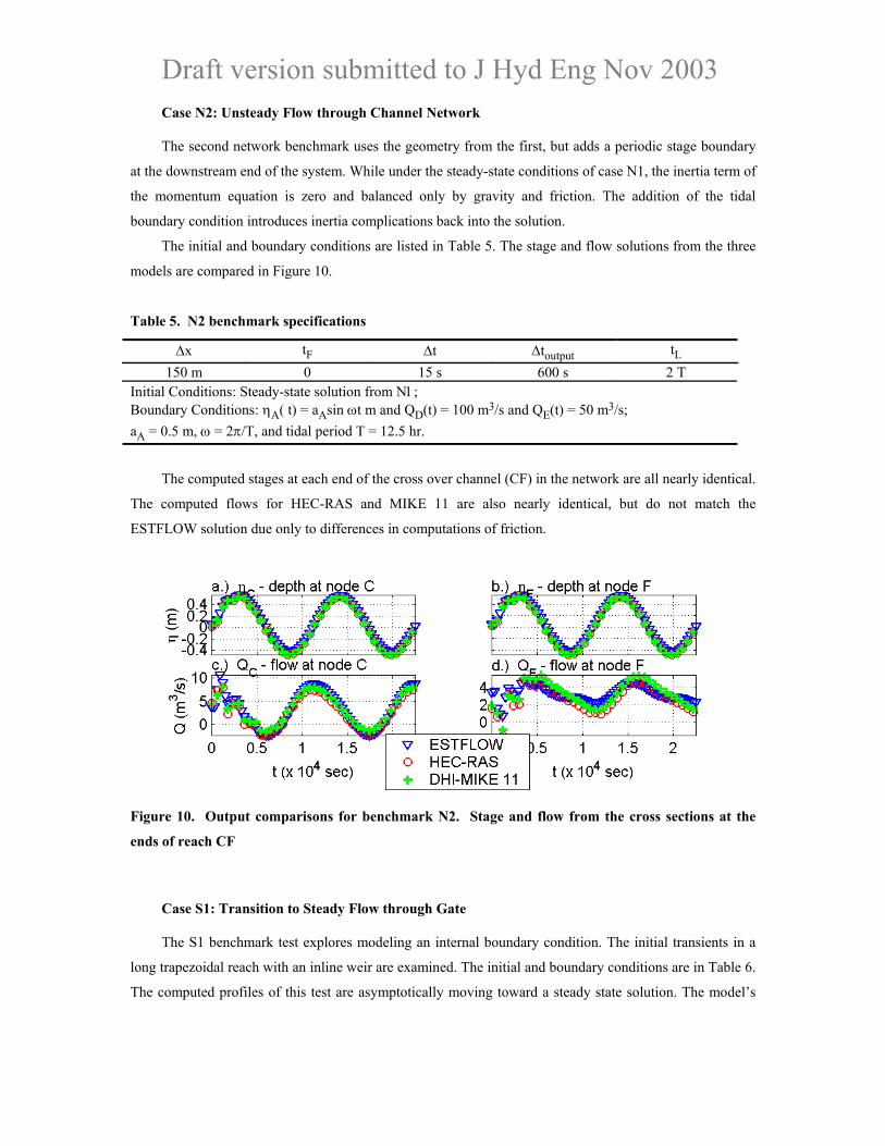
Draft version submitted to J Hyd Eng Nov 2003 Case N2: Unsteady Flow through Channel Network

The second network benchmark uses the geometry from the first, but adds a periodic stage boundary

at the downstream end of the system. While under the steady-state conditions of case N1, the inertia term of

the momentum equation is zero and balanced only by gravity and friction. The addition of the tidal

boundary condition introduces inertia complications back into the solution.

The initial and boundary conditions are listed in Table 5. The stage and flow solutions from the three

models are compared in Figure 10.

Table 5. N2 benchmark specifications

∆x tF ∆t ∆toutput tL 150 m 0 15 s 600 s 2 T

Initial Conditions: Steady-state solution from Ν1; Boundary Conditions: ηA( t) = aAsin ωt m and QD(t) = 100 m3/s and QE(t) = 50 m3/s; aA = 0.5 m, ω = 2π/T, and tidal period T = 12.5 hr.

The computed stages at each end of the cross over channel (CF) in the network are all nearly identical.

The computed flows for HEC-RAS and MIKE 11 are also nearly identical, but do not match the

ESTFLOW solution due only to differences in computations of friction.

Figure 10. Output comparisons for benchmark N2. Stage and flow from the cross sections at the

ends of reach CF

Case S1: Transition to Steady Flow through Gate

The S1 benchmark test explores modeling an internal boundary condition. The initial transients in a

long trapezoidal reach with an inline weir are examined. The initial and boundary conditions are in Table 6.

The computed profiles of this test are asymptotically moving toward a steady state solution. The model’s

Draft version submitted to J Hyd Eng Nov 2003 predictions are compared in Figure 11 and Figure 12 with profiles after 270 and 1170 seconds of

simulation.

Table 6. S1 benchmark specifications

xF ∆x xL zF zL BW SS tF ∆t ∆toutput tL 0 150 m 15,000 m -2 m -2 m 3 m 2 0 30 s 90 s 1.5 hr

Initial Conditions: η(x, 0) = 0 m and Q(x, 0) = 0 m3/s; Boundary Conditions: η(xL, t) = 0 m and Q(xF, t) = +100 m3/s; QF introduced by a linear ramp function over 30 s; Gate, xB = xC = 6000 m, W = 2.5 m, zsill = -1.5 m, CG = 0.5; n = 0.02

This test case has initial transients from two sources, from the rapid change in flow from 0 100

m3/sec and from the internal forced relationship between stage and flow over the gate. HEC-RAS, MIKE

11 and ESTFLOW produce a relatively similar propagation of the flow transition. The ESTFLOW solution,

as noted in the original paper, has regular oscillations and is explained as the expected free mode responses

bouncing off the internal boundary (gate). HEC-RAS and MIKE 11 would require a smaller time and

distance step to characterize this type of transient. The case study presented next demonstrates that HEC-

RAS and MIKE 11 are capable of modeling internal waves caused by a gate closure in a real system.

Figure 11. Profile comparison for benchmark S1 after 270 seconds

Figure 12. Profile comparison for benchmark S1 after 1170 seconds

Draft version submitted to J Hyd Eng Nov 2003 Case Study – San Joaquin Canal

The San Joaquin Canal is part of the agricultural distribution system in the Central Valley Project

(CVP) of California. The canal is a cascade of channels (referred to as pools by CVP) separated by gated

structures; the stage is measured at the upstream and downstream ends of the pool. The goal of the models

is to predict an observed transient generated from sequentially closing the gates on both ends of one of the

pools in the canal (DeVries et al., 1968).

Table 7. San Joaquin Canal specifications

xF ∆x xL zF zL BW SS tF ∆t ∆toutput tL 0 15.2 m 8,944 m 60.40 m 60.82 m 12.2 m 1.5 0 10 s 60 s 120 min

Gate size: Height = 6.1 m, Width = 12.2 m; Initial Conditions: η(x, 0) = 68.82 and Q(x, 0) = 48.1 m3/s; Boundary Conditions: η(xF, t) = 70.0 m and Q(xL, t) = 48.14 m3/s for t < 10 min Q(xL, t) = 0 m3/s for t > 11 minutes with linear drop over 1 min; Gate (at xF) Open Height = 0.80 m for t < 22 min and closes over 4 min; n = 0.016.

Wave Celerity and Expected Travel Time in the Canal: Average Hydraulic Depth = 5.33 m Wave Celerity = 7.23 m/s Travel Time ~ 20.5 min Round Trip Time ~ 41 min

The stage along the entire pool reach is shown in Figure 13 for 6 times. The upstream gate closure (t =

10 min) causes a drop in the stage at the upstream end of the pool that travels downstream. Before the wave

reaches the end of the pool, the downstream gate starts to close (t = 22 min), which also creates a run up

wave. Both waves combine on the downstream end of the canal and then reflect back to the upstream gate.

The wave reflects off the upstream gate and travels with a round trip time of 41 minutes.

The computed water surface elevations are compared to the observed water surface elevations at the

gages at the upstream and downstream end of the pool in Figure 14. Both models do a good job in

predicting the stage changes at each end of the pool reach.

Draft version submitted to J Hyd Eng Nov 2003

Figure 13. Stage along the entire reach at 6 times

Figure 14. Model predictions compared to observed values at the upstream and downstream ends of

the reach

CONCLUSIONS:

Sobey developed a series of benchmark tests for unsteady, one-dimensional, open channel flow

models. The tests ranged from simple single reach models to looped networks. Boundary conditions were

designed to be at the edge of expected stability. In spite of computational differences, both the HEC-RAS

and MIKE 11 models successfully demonstrated the ability to model these benchmark cases. For the rough

discretization in some of the benchmark tests, the MIKE 11 code demonstrated an ability to respond more

quickly to disturbances presented by the initial conditions.

In addition to the theoretical tests, HEC-RAS and MIKE 11 were applied to a measured transient

generated from closing gates in the San Joaquin canal. Both models performed well in simulating the

observed magnitude and speed of the transient waves as they combined and were reflected back and forth

along the canal.

Draft version submitted to J Hyd Eng Nov 2003 Properly applied to one-dimensional modeling projects, both HEC-RAS and MIKE 11 will produce

viable predictions.

REFERENCES:

Abbott, M.B. and F. Ionescu, 1967, On the numerical computation of nearly-horizontal flows, Journal of

Hydraulic Research, 5, pp. 97-117.

Danish Hydraulic Institute, 2001, MIKE 11 Reference manual, Appendix A. Scientific background,

Danish Hydraulic Institute.

DeVries, J.J., I.C. Tod, and T.V. Hromadka, 1968, Unsteady Canal Flow - Comparison of Simulations with

Field Data", ASCE Proc: International Symposium, "Model Prototype Correlation of Hydraulic

Structures”, Colorado Springs, pp 456-465.

HEC-RAS Hydraulic Reference Manual, Version 3.1 November 2002, available for download at

www.hec.usace.army.mil.

Sobey,R. J. 2001, Evaluation of Numerical Models of Flood and Tide Propagation in Channels, Journal of

Hydraulic Engineering, ASCE, Vol. 127 No 10, pp 805-824.

ACKNOWLEDGEMENTS:

The authors would like to thank Professor Rodney J. Sobey for the output used in his original paper and

Steve Piper at HEC and Morten Rungø at DHI for their assistance in modifying their respective models to

output the individual terms of the differential equations.

NOTATION:

The following symbols are sued in this paper:

A = local cross-sectional area of channel; BW = bottom width; b = local surface width of channel; g = gravitational acceleration; n = Manning friction coefficient; Q = discharge; S = slope; SS = side slopes (horizontal to 1 vertical); s = seconds; T = period; t = time; ∆t = time step; x = longitudinal position; ∆x = space step; z = bed elevation; η = water surface elevation; τ = shear stress; and ω = radian frequency.

Subscripts

Draft version submitted to J Hyd Eng Nov 2003 F = first; L = last; N = mode, timestep; n = normal depth; and 0 = bed.