
Draft Regulatory Impact Analysis - US Environmental Protection
391
Draft Regulatory Impact Analysis Proposed Rulemaking to Establish Green- house Gas Emissions Standards and Fuel Efficiency Standards for Medium- and Heavy-Duty Engines and Vehicles
Transcript of Draft Regulatory Impact Analysis - US Environmental Protection

Draft Regulatory Impact Analysis Proposed Rulemaking to Establish Green-house Gas Emissions Standards and Fuel Efficiency Standards for Medium- and Heavy-Duty Engines and Vehicles

EPA-420-D-10-901 October 2010
Office of Transportation and Air Quality U.S. Environmental Protection Agency
and
National Highway Traffic Safety Administration U.S. Department of Transportation
Draft Regulatory Impact Analysis
Proposed Rulemaking to Establish Green-house Gas Emissions Standards and Fuel Efficiency Standards for Medium- and
Heavy-Duty Engines and Vehicles
NOTICE This technical report does not necessarily represent final EPA decisions or positions. It is intended to present technical analysis of issues using data that are currently available. The purpose in the release of such reports is to facilitate the exchange of technical information and to inform the public of technical developments.

i
TABLE OF CONTENTS
EXECUTIVE SUMMARY CHAPTER 1: INDUSTRY CHARACTERIZATION 1.1 Introduction 1-1 1.2 Heavy-Duty Truck Categories 1-6 1.3 Heavy-Duty Truck Segments 1-8 1.4 Operations 1-14 1.5 Tire Manufacturers 1-26 1.6 Current U.S. and International GHG Voluntary Actions and Regulations 1-30 1.7 Trailers 1-33 1.8 Hybrids 1-37 CHAPTER 2: TECHNOLOGIES, COST, AND EFFECTIVENESS 2.1 Overview of Technologies 2-1 2.2 Overview of Technology Cost Methodology 2-2 2.3 Heavy-Duty Pickup Truck and Van Technologies and Costs 2-10 2.4 Heavy-Duty Engines 2-19 2.5 Class 7/8 Day Cabs and Sleeper Cabs 2-33 2.6 Class 2b-8 Vocational Vehicles 2-62 2.7 Air Conditioning 2-73 2.8 Trailers and GHG Emission Reduction Opportunities 2-76 2.9 Other Fuel Consumption and GHG Reducing Strategies 2-81 2.10 Summary of Technology Costs Used in this Analysis 2-89 CHAPTER 3: TEST PROCEDURES 3.1 Heavy-Duty Engine Test Procedure 3-1 3.2 Aerodynamic Assessment 3-5 3.3 Tire Rolling Resistance 3-20 3.4 Drive Cycle 3-22 3.5 Tare Weights and Payload 3-26 3.6 Heavy-Duty Chassis Test Procedure 3-29 3.7 Hybrid Powertrain Test Procedures 3-30 3.8 HD Pickup Truck and Van Chassis Test Procedure 3-41 CHAPTER 4: VEHICLE SIMULATION MODEL 4.1 Purpose and Scope 4-1 4.2 Model Code Description 4-2 4.3 Feasibility of Using a Model to Simulate Testing 4-4 4.4 EPA and NHTSA Vehicle Compliance Model 4-7 4.5 Application of Model for Certification 4-18 CHAPTER: 5 EMISSIONS IMPACTS 5.1 Executive Summary 5-1 5.2 Introduction 5-2 5.3 Program Analysis and Modeling Methods 5-4 5.4 Greenhouse Gas Emission Impacts 5-11 5.5 Non-Greenhouse Gas Emission Impacts 5-12

CHAPTER 6: RESULTS OF PROPOSED AND ALTERNATIVE STANDARDS 6.1 What Are the Alternatives that the Agencies Considered? 6-1 6.2 How Do These Alternatives Compare in Overall GHG Emissions Reductions and Fuel Efficiency and Cost? 6-14 CHAPTER 7: TRUCK COSTS AND COSTS PER TON OF GHG EMISSIONS REDUCED 7.1 Costs Associated with the Proposed Program 7-1 7.2 Cost per Ton of GHG Emissions Reduced 7-4 7.3 Impacts of Reduction in Fuel Consumption 7-6 7.4 Key Parameters Used in the Estimation of Costs and Fuel Savings 7-7 CHAPTER 8: HEALTH AND ENVIRONMENTAL IMPACTS 8.1 Health and Environmental Effects of Non-GHG Pollutants 8-1 8.2Air Quality Impacts of Non-GHG Pollutants 8-33 8.3 Quantified and Monetized Non-GHG Health and Environmental Impacts 8-38 8.4 Changes in Atmospheric CO2 Concentrations, Global Mean Temperature, Sea Level Rise, and Ocean pH Associated with the Proposal’s GHG Emissions Reductions 8-44 8.5 Monetized CO2 Impacts 8-52 CHAPTER 9. ECONOMIC AND SOCIAL IMPACTS 9.1 Framework for Benefits and Costs 9-1 9.2 Rebound Effect 9-2 9.3 Other Economic Impacts 9-12 9.4 The Effect of Safety Standards and Voluntary Safety Improvements on Vehicle Weight 9-17 9.5 Petroleum and energy security impacts 9-21 9.6 Summary of Benefits and Costs 9-32 CHAPTER 10. SMALL BUSINESS FLEXIBILITY ANALYSIS

List of Acronyms
2008$ U.S. Dollars in calendar year 2008 µg Microgram µg/m3 Microgram per Cubic Meter µm Micrometers AC Alternating Current ACES Advanced Collaborative Emission Study APU Auxiliary Power Unit AQCD Air Quality Criteria Document ASPEN Assessment System for Population Exposure Nationwide ATA American Trucking Association ATRI Alliance for Transportation Research Institute avg Average BAC Battery Air Conditioning BenMAP Benefits Mapping and Analysis Program bhp Brake Horsepower bhp-hrs Brake Horsepower Hours BTS Bureau of Transportation BTU British Thermal Unit CAA Clean Air Act CAE Computer Aided Engineering CAFE Corporate Average Fuel Economy CARB California Air Resources Board CCP Coupled Cam Phasing Cd Coefficient of Drag CDC Centers for Disease Control CFD Computational Fluid Dynamics CFR Code of Federal Regulations CH4 Methane CILCC Combined International Local and Commuter Cycle CITT Chemical Industry Institute of Toxicology CMAQ Community Multiscale Air Quality CO Carbon Monoxide CO Carbon Dioxide 2 COI Cost of Illness COPD Chronic Obstructive Pulmonary Disease CoV Coefficient of Variation CRGNSA Columbia River Gorge National Scenic Area CSI Cambridge Systematics Inc. CVD Cardiovascular Disease DE Diesel Exhaust DEAC Cylinder Deactiviation DEF Diesel Exhaust Fluid DHHS U.S. Department of Health and Human Services DOC Diesel Oxidation Catalyst DOE Department of Energy DOT Department of Transportation DPF Diesel Particulate Filter DPM Diesel Particulate Matter

DR Discount Rate DRIA Draft Regulatory Impact Analysis EC Elemental Carbon ED Emergency Department EGR Exhaust Gas Recirculation EIA Energy Information Administration (part of the U.S. Department of Energy) EMS-HAP Emissions Modeling System for Hazardous Air Pollution EO Executive Order EPA Environmental Protection Agency EPS Electric Power Steering EPS Electrified Parking Spaces ERG Eastern Research Group EV Electric Vehicle F Frequency FHWA Federal Highway Administration FIA Forest Inventory and Analysis FOH Fuel Operated Heater FR Federal Register g Gram g/ton-mile Grams emitted to move one ton (2000 pounds) of freight over one mile gal Gallon gal/1000 ton-mile Gallons of fuel used to move one ton of payload (2,000 pounds) over 1000 miles GDP Gross Domestic Product GEOS Goddard Earth Observing System GHG Greenhouse Gases GIFT Geospatial Intermodal Freight Transportation GUI Graphical User Interface GVW Gross Vehicle Weight Rating GWP Global Warming Potential HAD Diesel Health Assessment Document HC Hydrocarbon HD Heavy-Duty HDUDDS Heavy Duty Urban Dynamometer Driving Cycle HEI Health Effects Institute HES Health Effects Subcommittee HEV Hybrid Electric Vehicle HFET Highway Fuel Economy Dynamometer Procedure hp Horsepower hrs Hours HSC High Speed Cruise Duty Cycle HTUF Hybrid Truck User Forum hz Hertz IARC International Agency for Research on Cancer ICCT International Council on Clean Transport ICD International Classification of Diseases ICF ICF International IMPROVE Interagency Monitoring of Protected Visual Environments IRIS Integrated Risk Information System ISA Integrated Science Assessment JAMA Journal of the American Medical Association

k Thousand kg Kilogram km Kilometer kW Kilowatt L Liter lb Pound LD Light-Duty LSC Low Speed Cruise Duty Cycle m2 Square Meters m3 Cubic Meters MD Medium-Duty mg Milligram mi mile min Minute MM Million MOVES Motor Vehicle Emissions Simulator mpg Miles per Gallon mph Miles per Hour MSAT Mobile Source Air Toxic MY Model Year N2O Nitrous Oxide NA Not Applicable NAAQS National Ambient Air Quality Standards NAICS North American Industry Classification System NAS National Academy of Sciences NATA National Air Toxic Assessment NCAR National Center for Atmospheric Research NCI National Cancer Institute NCLAN National Crop Loss Assessment Network NEC Net Energy Change Tolerance NEI National Emissions Inventory NESCCAF Northeast States Center for a Clean Air Future NESHAP National Emissions Standards for Hazardous Air Pollutants NHTSA National Highway Traffic Safety Administration NiMH Nickel Metal-Hydride NIOSH National Institute of Occupational Safety and Health NMHC Nonmethane Hydrocarbons NMMAPS National Morbidity, Mortality, and Air Pollution Study NO Nitrogen Oxide NO Nitrogen Dioxide 2 NOAA National Oceanic and Atmospheric Administration NOx Oxides of Nitrogen NPRM Notice of Proposed Rulemaking NPV Net Present Value NRC National Research Council NVH Noise Vibration and Harshness O&M Operating and maintenance O Ozone 3 OAQPS Office of Air Quality Planning and Standards OC Organic Carbon

OE Original Equipment OEHHA Office of Environmental Health Hazard Assessment OEM Original Equipment Manufacturer OHV Overhead Valve OMB Office of Management and Budget ORD EPA's Office of Research and Development OTAQ Office of Transportation and Air Quality Pa Pascal PAH Polycyclic Aromatic Hydrocarbons PEMS Portable Emissions Monitoring System PHEV Plug-in Hybrid Electric Vehicles PM Particulate Matter PM10 Coarse Particulate Matter (diameter of 10 µm or less) PM2.5 Fine Particulate Matter (diameter of 2.5 µm or less) POM Polycyclic Organic Matter ppb Parts per Billion ppm Parts per Million psi Pounds per Square Inch PTO Power Take Off R&D Research and Development RBM Resisting Bending Moment RESS Rechargeable Energy Storage System RfC Reference Concentration RIA Regulatory Impact Analysis rpm Revolutions per Minute RRc Rolling Resistance Coefficient SAB Science Advisory Board SAB-HES Science Advisory Board - Health Effects Subcommittee SAE Society of Automotive Engineers SBA Small Business Administration SBAR Small Business Advocacy Review SBREFA Small Business Regulatory Enforcement Fairness Act SCC Social Cost of Carbon SCR Selective Catalyst Reduction SER Small Entity Representation SGDI Stoichiometric Gasoline Direct Injection SIDI Spark Ignition Direct Injection SO Sulfur Dioxide 2 SOC State of Charge SOHC Single Overhead Cam SOx Oxides of Sulfur STB Surface Transportation Board SUV Sport Utility Vehicle SVOC Semi-Volatile Organic Compound TIAX TIAX LLC Ton-mile One ton (2000 pounds) of payload over one mile TRU Trailer Refrigeration Unit TSD Technical Support Document TSS Thermal Storage U/DAF Upward and Downward Adjustment Factor

UCT Urban Creep and Transient Duty Cycle UFP Ultra Fine Particles USDA United States Department of Agriculture UV Ultraviolet UV-b Ultraviolet-b VIUS Vehicle Inventory Use Survey VMT Vehicle Miles Travelled VOC Volatile Organic Compound VSL Value of Statistical Life VVT Variable Valve Timing WTP Willingness-to-Pay WTVC World Wide Transient Vehicle Cycle WVU West Virginia University

This Page Intentionally Left Blank

ES-1
Executive Summary The Environmental Protection Agency (EPA) and the National Highway Traffic Safety
Administration (NHTSA), on behalf of the Department of Transportation, are each proposing rules to establish a comprehensive Heavy-Duty National Program that would reduce greenhouse gas emissions and increase fuel efficiency for on-road heavy-duty vehicles, responding to the President’s directive on May 21, 2010, to take coordinated steps to produce a new generation of clean vehicles. NHTSA’s proposed fuel consumption standards and EPA’s proposed carbon dioxide (CO2) emissions standards would be tailored to each of three regulatory categories of heavy-duty vehicles: (1) Combination Tractors; (2) Heavy-duty Pickup Trucks and Vans; and (3) Vocational Vehicles, as well as gasoline and diesel heavy-duty engines. EPA’s proposed hydrofluorocarbon emissions standards would apply to air conditioning systems in tractors, pickup trucks, and vans, and EPA’s proposed nitrous oxide (N2O) and methane (CH4
Table 1 presents the rule-related benefits, costs and net benefits in both present value terms and in annualized terms. In both cases, the discounted values are based on an underlying time varying stream of cost and benefit values that extend into the future (2012 through 2050). The distribution of each monetized economic impact over time can be viewed in the RIA Chapters that follow this summary.
) emissions standards would apply to all heavy-duty engines, pickup trucks, and vans.
Present values represent the total amount that a stream of monetized costs/benefits/net benefits that occur over time are worth now (in year 2008 dollar terms for this analysis), accounting for the time value of money by discounting future values using either a 3 or 7 percent discount rate, per OMB Circular A-4 guidance. An annualized value takes the present value and converts it into a constant stream of annual values through a given time period (2012 through 2050 in this analysis) and thus averages (in present value terms) the annual values. The present value of the constant stream of annualized values equals the present value of the underlying time varying stream of values. Comparing annualized costs to annualized benefits is equivalent to comparing the present values of costs and benefits, except that annualized values are on a per-year basis.
It is important to note that annualized values cannot simply be summed over time to reflect total costs/benefits/net benefits; they must be discounted and summed. Additionally, the annualized value can vary substantially from the time varying stream of cost/benefit/net benefit values that occur in any given year (e.g., the stream of costs represented by $0.34B and $0.58B in Table 1 below average $1.5B from 2014 through 2018 and are zero from 2019-2050).
Table 1 Estimated Lifetime and Annualized Discounted Costs, Benefits, and Net Benefits for 2014-2018 Model Year HD Vehicles assuming the $22/ton SCC Valuea,b
LIFETIME PRESENT VALUE
(billions 2008 dollars)
C,D
Costs – 3% DISCOUNT RATE
$7.7

ES-2
Benefits $49
Net Benefits $41
Annualized valuec,e
Costs – 3% Discount Rate
$0.34
Benefits $2.1
Net Benefits $1.8
Lifetime Present valuec,d
Costs
- 7% Discount Rate
$7.7
Benefits $34
Net Benefits $27
Annualized valuec,e
Costs – 7% Discount Rate
$0.58
Benefits $2.6
Net Benefits $2.0
Notes: a Although the agencies estimated the benefits associated with four different values of a one ton CO2 reduction (SCC: $5, $22, $36, $66), for the purposes of this overview presentation of estimated costs and benefits we are showing the benefits associated with the marginal value deemed to be central by the interagency working group on this topic: $22 per ton of CO2, in 2008 dollars and 2010 emissions and fuel consumption. As noted in Section VIII.G, SCC increases over time. b Note that net present value of reduced GHG emissions is calculated differently than other benefits. The same discount rate used to discount the value of damages from future emissions (SCC at 5, 3, and 2.5 percent) is used to calculate net present value of SCC for internal consistency. Refer to Section VIII.G for more detail. c Discounted values presented in this table are based on an underlying series of cost and benefit values that extend into the future (2012 through 2050). The distribution of each monetized economic impact over time can be viewed in the RIA that accompanies this preamble. d Present value is the total, aggregated amount that a series of monetized costs or benefits that occur over time is worth now (in year 2008 dollar terms), discounting future values to the present. e
This Regulatory Impact Analysis (RIA) provides detailed supporting documentation to the EPA and NHTSA joint proposal under each of their respective statutory authorities. Because there are slightly different requirements and flexibilities in the two authorizing statutes, this RIA
The annualized value is the constant annual value through a given time period (2012 through 2050 in this analysis) whose summed present value equals the present value from which it was derived.
ES-3
provides documentation for the primary joint proposed provisions as well as for provisions specific to each agency.
The agencies request comment on the methods and assumptions used to estimate costs, benefits, and technology cost-effectiveness for the main proposal and all of the alternatives. The agencies also seek comment on whether finalizing a different alternative stringency level for certain regulatory categories would be appropriate given agency estimates of costs and benefits.
This RIA is generally organized to provide overall background information, methodologies, and data inputs, followed by results of the various technical and economic analyses. A summary of each chapter of the RIA follows.
Chapter 1: Industry Characterization. In order to assess the impacts of greenhouse gas (GHG) and fuel efficiency regulations upon the affected industries, it is important to understand the nature of the industries impacted by the regulations. The heavy-duty vehicle industries include the manufacturers of Class 2b through Class 8 trucks, engines, and some equipment. This chapter provides market information for each of these affected industries, as well as the variety of ownership patters, for background purposes. Vehicles in these classes range from over 8,500 pounds (lbs) gross vehicle weight rating (GVWR) to upwards of 80,000 lbs and can be used in applications ranging from ambulances to vehicles that transport the fuel that powers them. The heavy-duty segment is very diverse both in terms of its type of vehicles and vehicle usage patterns. Unlike the light-duty segment whose primary mission tends to be transporting passengers for personal travel, the heavy duty segment has many different missions. Some pickup trucks may be used for personal transportation to and from work with an average annual mileage of 15,000 miles. Class 7 and 8 combination tractors are primarily used for freight transportation, can carry up to 50,000 pounds of payload, and can travel more than 150,000 miles per year.
Chapter 2: Technology Packages, Cost and Effectiveness. This chapter presents details of the vehicle and engine technology packages for reducing greenhouse gas emissions and fuel consumption. These packages represent potential ways that the industry could meet the proposed CO2
Chapter 3: Test Procedures. Laboratory procedures to physically test engines, vehicles, and components are a crucial aspect of the proposed heavy-duty vehicle GHG and fuel consumption program. The proposed rulemaking would establish several new test procedures for both engine and vehicle compliance. This chapter describes the development process for the test procedures being proposed, including methodologies for assessing engine emission performance, the effects of aerodynamics and tire rolling resistance, as well as procedures for chassis dynamometer testing and their associated drive cycles.
and fuel consumption stringency levels, and they provide the basis for the technology costs and effectiveness analyses.
Chapter 4: Vehicle Simulation Model. An important aspect of a regulatory program is its ability to accurately estimate the potential environmental benefits of heavy-duty truck technologies through testing and analysis. Most large truck manufacturers employ various computer simulation methods to estimate truck efficiency. Each method has advantages and disadvantages. This section will focus on the use of a type truck simulation modeling that the

ES-4
agencies have developed specifically for assessing tailpipe GHG emissions and fuel consumption for purposes of this rulemaking. The agencies are proposing to use this newly-developed simulation model -- the “Greenhouse gas Emissions Model (GEM)” -- as the primary tool to certify vocational and combination tractor heavy-duty vehicles (Class 2b through Class 8 heavy-duty vehicles that are not heavy-duty pickups or vans) and discuss the model in this chapter.
Chapter 5: Emissions Impacts. This proposal estimates anticipated impacts from the proposed CO2 emission and fuel efficiency standards. The agencies quantify emissions from the GHGs carbon dioxide (CO2), methane (CH4), nitrous oxide (N2O) and hydrofluorocarbons (HFCs). In addition to reducing the emissions of greenhouse gases and fuel consumption, this proposal would also influence the emissions of “criteria” air pollutants, including carbon monoxide (CO), fine particulate matter (PM2.5) and sulfur dioxide (SOX) and the ozone precursors hydrocarbons (VOC) and oxides of nitrogen (NOX
The agencies used EPA’s Motor Vehicle Emission Simulator (MOVES2010) to estimate downstream (tailpipe) emission impacts, and a spreadsheet model based on emission factors the “GREET” model to estimate upstream (fuel production and distribution) emission changes resulting from the decreased fuel. Based on these analyses, the agencies estimate that this proposal would lead to 72 million metric tons (MMT) of CO
); and several air toxics (including benzene, 1,3-butadiene, formaldehyde, acetaldehyde, and acrolein), as described further in Chapter 5.
2 equivalent (CO2
Chapter 6: Results of Proposed and Alternative Standards. The heavy-duty truck segment is very complex. The sector consists of a diverse group of impacted parties, including engine manufacturers, chassis manufacturers, truck manufacturers, trailer manufacturers, truck fleet owners and the public. The agencies have largely designed this proposal to maximize the environmental and fuel savings benefits of the program, taking into account the unique and varied nature of the regulated industries. In developing this proposal, we considered a number of alternatives that could have resulted in fewer or potentially greater GHG and fuel consumption reductions than the program we are proposing. Chapter 6 section summarizes the alternatives we considered.
EQ) of annual GHG reduction and 5.8 billion gallons of fuel savings in the year 2030, as discussed in more detail in Chapter 5.
Chapter 7: Truck Costs and Costs per Ton of GHG. In this chapter, the agencies present our estimate of the costs associated with the proposed program. The presentation summarizes the costs associated with new technology expected to be added to meet the proposed GHG and fuel consumption standards, including hardware costs to comply with the air conditioning (A/C) leakage program. The analysis discussed in Chapter 7 provides our best estimates of incremental costs on a per truck basis and on an annual total basis.
Chapter 8: Environmental and Health Impacts. This chapter discusses the health effects associated with non-GHG pollutants, specifically: particulate matter, ozone, nitrogen oxides (NOX), sulfur oxides (SOX), carbon monoxide and air toxics. These pollutants would not be directly regulated by the standards, but the standards would affect emissions of these pollutants and precursors. Reductions in these pollutants would be co-benefits of the final rulemaking (that is, benefits in addition to the benefits of reduced GHGs).

ES-5
Chapter 9: Economic and Social Impacts. This chapter provides a description of the net benefits of the proposed HD National Program. To reach these conclusions, the chapter discusses each of the following aspects of the analyses of benefits:
Rebound Effect: The VMT rebound effect refers to the fraction of fuel savings expected to result from an increase in fuel efficiency that is offset by additional vehicle use.
Energy Security Impacts: A reduction of U.S. petroleum imports reduces both financial and strategic risks associated with a potential disruption in supply or a spike in cost of a particular energy source. This reduction in risk is a measure of improved U.S. energy security.
Other Impacts: There are other impacts associated with the proposed GHG emissions and fuel efficiency standards. Lower fuel consumption would, presumably, result in fewer trips to the filling station to refuel and, thus, time saved. The increase in vehicle-miles driven due to a positive rebound effect may also increase the societal costs associated with traffic congestion, motor vehicle crashes, and noise. The agencies also discuss the impacts of safety standards and voluntary safety improvements on vehicle weight.
Chapter 9 also presents a summary of the total costs, total benefits, and net benefits expected under the proposal.
Chapter 10: Small Business Flexibility Analysis. This chapter describes the agencies’ analysis of the small business impacts due to the joint proposal.

Heavy-Duty GHG and Fuel Efficiency Standards NPRM: Industry Characterization
1-1
Chapter 1: Industry Characterization 1.1 Introduction
1.1.1 Overview
In order to assess the impacts of greenhouse gas (GHG) regulations upon the affected industries, it is important to understand the nature of the industries impacted by the regulations. These industries include the manufacturers of Class 2b through Class 8 trucks, engines, and some equipment. This chapter provides market information for each of these affected industries for background purposes. Vehicles in these classes range from over 8,500 pounds (lbs) gross vehicle weight rating (GVWR) to upwards of 80,000 lbs and can be used in applications ranging from ambulances to vehicles that transport the fuel that powers them. Figure 1-1 shows the difference in vehicle classes in terms of GVWR and the different applications found in these classes.
Figure 1-1 Description and Weight Ratings of Vehicle Classes
Source: Commercial Carrier Journal http://www.ccjmagazine.com

Regulatory Impact Analysis
1-2
Heavy-duty trucks in this rulemaking are defined as on-highway vehicles with a GVWR greater than 8,500 lbs and are not defined as Medium-Duty Passenger Vehicles (MDPV). The EPA and NHTSA jointly developed the Light-Duty Vehicle Greenhouse Gas Emissions Standards and Corporate Average Fuel Economy Standards; Final Rule 75 FR 25323 (May 7, 2010) which sets standards for Light Duty Vehicles, Light-Duty Trucks, and Medium-Duty Passenger Vehicles (EPA-420-F-10-014). Light-duty trucks are vehicles with GVWR less than 8,500 lbs. MDPV are vehicles with GVWR less than 10,000 pounds which meet the criteria outlined in 40 C.F.R. §86.1803-01. This grouping typically includes large sport utility vehicles, small trucks, and mini-vans.
The heavy-duty segment is very diverse both in terms of its type of vehicles and vehicle usage patterns. Unlike the light-duty segment whose primary mission tends to be transporting passengers for personal travel, the heavy duty segment has many different missions. Some pickup trucks may be used for personal transportation to and from work with an average annual mileage of 15,000 miles. Class 7 and 8 combination tractors are primarily used for freight transportation, can carry up to 50,000 pounds of payload, and can travel more than 150,000 miles per year. For the purposes of this report, heavy-duty segment has been separated as follows: Class 2b and 3 pickup trucks and vans (also referred to as HD pickup trucks and vans), Class 2b through 8 vocational vehicles, Class 7 and 8 combination tractors, trailers, and transit buses.
1.1.2 Freight Moved by Heavy-Duty Trucks
In 2008, heavy-duty trucks carried more freight in terms of tonnage and value in the U.S. than all other modes of freight transportation combined, and are expected to move freight at an even greater rate in the future.1 According to the U.S. Department of Transportation (DOT), the U.S. transportation system moved, on average an estimated 59 million tons of goods worth an estimated $55 billion (in U.S. $2008) per day in 2008, or over 21 billion tons of freight worth more than $20 trillion in the year 2008.2 Of this, trucks moved over 13 billion tons of freight worth an estimated $13 trillion in 2008, or an average of nearly 36 million tons of freight worth $37 billion a day. The DOT’s Freight Analysis Framework estimates that this tonnage will increase nearly 73 percent by 2035, and that the value of the freight moved is increasing faster than the tons transported. Figure 1-2 shows the total tons of freight moved by each mode of freight transportation in 2002, 2008 and projections for 2035.

Heavy-Duty GHG and Fuel Efficiency Standards NPRM: Industry Characterization
1-3
Figure 1-2 Total Weight of Shipments by Transportation Mode (millions of tons)
1.1.3 Greenhouse Gas Emissions from Heavy-Duty Vehicles
The importance of this proposed rulemaking is highlighted by the fact that heavy-duty trucks are the largest source of GHG emissions in the transportation sector after light-duty vehicles. This sector represents approximately 22 percent of all transportation related GHG emissions as shown in Figure 1-3. Heavy-duty trucks are also a fast growing source of GHG emissions; total GHG emissions from this sector increased over 72 percent from 1990-2008 while GHG emissions from passenger cars grew approximately 20 percent over the same period.3 Available technologies developed through EPA’s SmartWay program and through DOE’s 21st Century Truck Partnership can achieve reductions from 10-20 percent and are applicable to the majority of heavy-duty vehicles; examples of these technologies include aerodynamic bumpers, mirrors, and fairings.4
Source: U.S. DOT, Federal Highway Administration, “Freight Facts and Figures
Notes: [a] Intermodal includes U.S. Postal Service and courier shipments and all intermodal combinations, except air and truck. Intermodal also includes oceangoing exports and imports that move between ports and interior domestic locations by modes other than water. [b] Pipeline also includes unknown shipments as data on region-to-region flows by pipeline are statistically uncertain.

Regulatory Impact Analysis
1-4
Figure 1-3 Transportation Related Greenhouse Gas Emissions (Tg CO2 Eq.) in 2008
1.1.4 Fuel Economy of Heavy-Duty Vehicles
While there is a corporate average fuel economy (CAFE) program for light-duty trucks and vehicles, the nature of the commercial truck market can present complications to such a structure in particular due to the production process, diversity of products, and usage patterns. 5 For example, in the light-duty market a manufacturer builds a complete vehicle and therefore, is responsible to certify that vehicle. In the heavy-duty truck market, there may be separate: chassis, engine, body and equipment manufacturers that contribute to the build process of a single truck; in addition, there are no companies that produce trucks and trailers and a given tractor may pull hundreds of different trailer types over the course of its life. Further, fuel economy is highly dependent on the configuration of a truck, for example: the type of body or box, engine, axle/gear ratios, cab, or other equipment installed on the vehicle; whether or not a truck carries cargo or has a specialized function (e.g. a bucket truck). Due to the varying needs of the industry, many of these trucks are custom built resulting in literally thousands of different truck configuration. Finally, usage patterns and duty cycles also greatly affect fuel economy, for example how trucks are loaded (cubed or weighed out) and how they are driven (delivery trucks travel at lower speeds and make frequent stops compared to a line-haul combination tractor). The potential to reduce fuel consumption, therefore, is also highly dependent on the truck configuration and usage.
Source: U.S. EPA, Inventory of Greenhouse Gas Emissions and Sinks: 1990-2008, published April, 2010

Heavy-Duty GHG and Fuel Efficiency Standards NPRM: Industry Characterization
1-5
The agencies recognize that while historic fuel economy and GHG emissions on a mile per gallon basis from heavy-duty trucks has been largely flat for more than 30 years, we cannot conclude with certainty that future improvements absent regulation would not occur.A Programs like EPA’s SmartWay program are not only helping the industry improve logistics and operations, but are also helping to encourage greater use of truck efficiency technologies. Looking at the total fuel consumed, total miles traveled, and total tons shipped in the U.S. or the average payload specific fuel consumption for the entire heavy-duty fleet from 1975 through 2005, the amount of fuel required to move a given amount of freight a given distance has been reduced by more than half as a result of improvements in technology, as shown in Figure 1-4.
Figure 1-4 U.S. Average Payload-Specific Fuel Consumption of the Heavy-Duty Fleet
5
Currently, manufacturers of vehicles with a GVW of over 8,500 pounds are not required to test and report fuel economy values, however, fuel economy ranges as of 2007 by vehicle class are presented in a study completed by the National Academy of Sciences (NAS), the U.S. Department of Transportation (DOT), and the National Highway Traffic Safety Administration (NHTSA). As one would expect, the larger the truck class the lower the fuel economy, for example, a typical mile per gallon (mpg) estimate for Class 2b vehicle is 10-15 mpg where a typical Class 8 combination tractor is estimated to get 4-7.5 mpg, as shown in Table 1-1.
A Over the last 30 years the average annual improvement in fuel economy has been 0.09%. See U. S. Department of Transportation, Federal Highway Administration, Highway Statistics 2008, Washington, DC, 2009, Table VM1 averaging annual performance for the years from 1979-2008.
(Source: NAS, Technologies and Approaches to Reducing Fuel Consumption of Medium- and Heavy-Duty Vehicles available here: http://www.nap.edu/openbook.php?record_id=12845&page=R1)

Regulatory Impact Analysis
1-6
Table 1-1 Estimated Fuel Economy by Truck Class
CLASS EXAMPLE PRODUCTION
VEHICLE
GVW TYPICAL MPG RANGE
IN 2007
TYPICAL TON-MPG
ANNUAL FUEL CONSUMPTION RANGE
(THOUSANDS OF GALLONS)
2b Dodge Ram 2500 Pickup Truck
8,501-10,000 10-15 26 1.5-2.7
3 Chevrolet Silverado 3500 Pickup Truck
10,001-14,000 8-13 30 2.5-3.8
4 Ford F-450 14,001-16,000 7-12 42 2.9-5.0 5 Kenworth T170 16,001-19,500 6-12 39 3.3-5.0 6 Peterbilt Model 330 19,501-26,000 5-12 49 5.0-7.0 7 Kenworth T370 26,001-33,000 4-8 55 6.0-8.0 8 Combination Trucks
International Lone Star 33,001-80,000 4-7.5 155 19 - 27
8 Other Mack Granite GU814 33,001-80,000 2.5-6 115 10 - 13
1.2 Heavy-Duty Truck Categories
This program addresses vehicles that fall into the following four categories: HD pickups and vans (typically Class 2b and 3), Vocational vehicles (typically Class 2b-8), Tractors (typically Class 7 and 8), and Heavy-Duty engines.B Class 2b and 3 pickups and vans are used for commercial purposes such as ambulances, shuttle buses, etc. The U.S. Energy Information Administration (EIA) estimates that Class 2b vehicles get approximately 14.5 – 15.6 miles per gallon (mpg) in 2010.6 Class 2b-8 vocational vehicles encompass a wide range of heavy-duty vehicles such as delivery trucks, school buses, etc. Fuel economy estimates for Class 3-6 are 7.8 mpg in 2010.7 Class 8 combinations tractors operate as either short-haul or long-haul trucks. Combination tractors that operate as short-haul trucks also known as day cabs, are tractor trailers that do not have sleeping quarters for the driver and haul trailers only short distances, typically into metropolitan areas. Combination tractors that operate as long-haul trucks are those equipped with sleeping quarters for the driver, and tend to drive well over 1,000 miles per trip; this category contributed the most GHG emissions of these four categories at just over 38 percent of the total CO2
Figure 1-5 emissions in
2005 as shown in . The EIA estimates that in 2010, Class 8 freight hauling trucks get slightly over 6 mpg.
B For purposes of this document, the term “heavy-duty” or “HD” is used to apply to all highway vehicles and engines that are not within the range of light-duty vehicles, light-duty trucks, and medium-duty passenger vehicles (MDPV) covered by the GHG and Corporate Average Fuel Economy (CAFE) standards issued for model years (MY) 2012-2016. Unless specified otherwise, the heavy-duty category incorporates all vehicles rated at a gross vehicle weight of 8,500 pounds, and the engines that power them, except for MDPVs.

Heavy-Duty GHG and Fuel Efficiency Standards NPRM: Industry Characterization
1-7
Figure 1-5 Tons of CO2 Emitted from Heavy-Duty Trucking in 2005
1.2.1 Heavy-Duty Vehicles Sales
Although not first in terms of GHG emissions, Class 2b and 3 pickup trucks and vans are first in terms of sales volumes, with sales of over 1.3 million units in 2005, or nearly 66 percent of the heavy-duty market. Sales of Class 3-8 vocational vehicles are the second most numerous, selling over one-half million units in 2005, or nearly 25 percent of the heavy-duty market. Since 2005, sales of all heavy-duty trucks have decreased as the economy contracted; the U.S. EPA’s MOVES model based on proprietary sales projections combined with the U.S. Energy Information Administration’s Annual Energy Outlook reflects a slow recovery in sales. Figure 1-6 and Figure 1-7 show the sales volumes for 2005 and projected sales for 2014 respectively, reflecting the market slowdown and recovery, while Table 1-2 shows sales projections by market segment for 2014-2018.
Table 1-2 Sales Projection by Market Segment 2014-2018
SALES ESTIMATES
2B/3 PICKUPS/VANS
VOCATIONAL VEHICLES
COMBINATION SHORT HAUL
COMBINATION LONG HAUL
TOTAL
2014 785,000 555,000 50,000 73,000 1,460,000
2015 730,000 573,000 50,000 74,000 1,430,000
2016 713,000 592,000 51,000 75,000 1,430,000
2017 708,000 611,000 52,000 77,000 1,450,000
2018 717,000 630,000 53,000 78,000 1,480,000

Regulatory Impact Analysis
1-8
Figure 1-6 2005 Heavy-Duty Truck Sales by Category
Figure 1-7 Projected Truck Sales for 2014 by Category
1.3 Heavy-Duty Truck Segments
1.3.1 Heavy-Duty Pickup Trucks and Vans
Class 2b and 3 pickup trucks and vans rank highest in terms of sales volumes, but together make up the third largest sector contributing to the heavy-duty truck GHG emissions (Class 2b through Class 8). There are number of reasons to explain this difference, but mainly it is the vehicle usage patterns and engine size. Class 2b/3 consists of pickup trucks and vans with a GVW between 8,500 and 14,000 pounds. Class 2b/3 truck manufacturers are predominately GM, Ford, and Chrysler, with Isuzu, Daimler, Mitsubishi FUSO, and Nissan

Heavy-Duty GHG and Fuel Efficiency Standards NPRM: Industry Characterization
1-9
also offering vehicles in this market segment. Figure 1-8 shows two examples of this category, a GM Chevrolet Express G3500 and a Dodge Ram 3500HD.
Figure 1-8 Examples of Class 2b and 3 Pickup Trucks and Vans
Class 2b/3 vehicles are sold either as complete or incomplete vehicles. For example a ‘complete vehicle’ can be a chassis cab (engine, chassis, wheels, and cab) or a rolling chassis (engine, chassis and wheels), while an ‘incomplete chassis’ could be sold as an engine and chassis only - no wheels. The technologies that can be used to reduce GHG emissions from this segment are very similar to the ones used for lighter pickup trucks and vans (Class 2a), which are part of the Light Duty GHG program. These technologies include engine improvements such as friction reduction, cylinder deactivation, cam phasing, and gasoline direct injection; aerodynamic improvements; low rolling resistance tires; and transmission improvements. The Class 2b/3 gasoline trucks and vans are currently certified with chassis dynamometer testing. The Class 2b/3 diesel trucks have an option to certify using the chassis dynamometer test procedure.
1.3.2 Vocational Vehicles
This market segment includes a wide range of heavy-duty vehicles ranging from 8,501 pounds to greater than 33,000 pounds GVW. In 2005, sales of these vehicles were the second most numerous sold in the heavy-duty truck market, with over 500,000 units sold, making up nearly one-quarter of all heavy-duty truck sales. The vocational vehicle segment was also responsible for emitting 15.3 percent of the GHG emissions in 2005 from the total heavy-duty truck market. A majority of these vehicles are powered by diesel engines; primary examples of this truck type include delivery trucks, dump trucks, cement trucks, buses, cranes, etc. Figure 1-9 shows two examples of this vehicle category including a United Parcel Service (UPS) delivery truck, and a Ford F750 Bucket Truck.

Regulatory Impact Analysis
1-10
Figure 1-9 Examples of Class 3-8 Vocation Truck Applications
Class 2b – 8 vocational vehicles are typically sold as an incomplete chassis with
multiple “outfitters” for example, an engine manufacturer, a body manufacturer, and an equipment manufacturer (e.g. a crane manufacturer). Manufacturers of vehicles within this segment vary widely and shift with class, as Figure 1-10 highlights. Vocational vehicles manufacturers include: GM, Ford, Chrysler, Isuzu, Mitsubishi, Volvo, Daimler, International, and PACCAR, while engine manufacturers include: Cummins, GM, Navistar, Hino, Isuzu, Volvo, Detroit Diesel, and PACCAR. Manufacturers of vocational vehicle bodies are numerous, according to the 2002 Census, there were 759 companies classified under the North American Industry Classification System (NAICS) 336211, “Motor Vehicle Body Manufacturers,” examples of these companies include: Utilimaster and Heller Truck Body Corp.
Opportunities for GHG reductions can include both engine and vehicle improvements. Currently, there are a limited number of available Class 2b-8 vocational vehicles produced in a hybrid configuration. International (owned by Navistar) makes the DuraStar™ Hybrid and claims that this option offers a 30 to 40 percent fuel economy benefit over standard in-city pickup and delivery applications, and offers a more than a 60 percent increase in fuel economy in utility-type applications where the vehicle can be shut off while electric power still operates the vehicle.8
www.seedmagazine.com/images/uploads/upstr
www.versalifteast.com/Rent-Bucket-Trucks.htm

Heavy-Duty GHG and Fuel Efficiency Standards NPRM: Industry Characterization
1-11
Figure 1-10 Class 3-8 Vocational Vehicle Manufacturer Shift with Class
Source: ICCT
1.3.3 Tractors
Class 7 and 8 trucks are the largest and most powerful trucks of the heavy duty vehicle fleet. These trucks use almost two-thirds of all truck fuel, and are typically categorized into two smaller segments – short-haul and long-haul. 9
Long-haul combination tractors typically travel at least 1,000 miles along a trip route. Long-haul operation occurs primarily on highways and accounts for 60 to 70 percent of the fuel use in this class. The remaining 30 to 40 percent of fuel is used by other short-and medium-haul regional applications.
Combination tractors operating as short-haul trucks are tractor trailers typically used for routes less than 500 miles, and tend to travel at lower average speeds than long-haul trucks. Short-haul combination tractors therefore, do not include sleeping accommodations for the driver.
10
Figure 1-11
The most common trailer hauled by both short- and long-haul combination tractors is a 53-foot dry box van trailer, which accounts for nearly 60 to 70 percent of heavy-duty Class 8 on-road mileage. Leading U.S. manufacturers of Class 8 trucks include companies such as International, Freightliner, Peterbilt, PACCAR, Kenworth, Mack, Volvo, and Western Star; while common engine manufacturers include companies such as Cummins, Navistar, and Detroit Diesel. shows example Class 8 day cab and sleeper cab combination tractors. The price of a new Class 8 vehicle can range from $90,000 to well over $110,000 for fully equipped models.11

Regulatory Impact Analysis
1-12
Figure 1-11 Example Day Cab and Sleeper Cab Tractors
1.3.4 Buses
Buses generally fall into either Class 6 or Class 7 categories and can come in many forms, including: transit buses, large school buses, small school buses, and motorcoaches. Typically, most bus manufacturers assemble the entire chassis from systems manufactured by a variety of suppliers, while their engines are commonly manufactured by companies such as Detroit Diesel, and Navistar.12 Typically, transit buses have about a 12 year lifespan, and approximately 5000-5500 units a year enter the fleet, where school buses can last upwards of fifteen years or longer as school buses are not eligible for Federal Transit Administration funding as most transit buses are.13
In 2008, transit buses were responsible for moving 53 percent of all unlinked passenger mass-transit trips which is just over 5.5 billion passenger trips.
Currently, about 32 percent of U.S. buses have an alternative energy source and are powered by a source other than diesel or gas. According to the American Public Transportation Association's (APTA) “2008 Public Transportation Fact Book,” in 2007, 22 percent of approximately 80,000 transit buses operated on alternative power, primarily compressed or liquefied natural gas (as well as recent interest in and growth of hybrid electric buses). Additionally, according to the Union of Concerned Scientists’ “School Bus Pollution Report Card 2006 Grading the Schools” (May, 2006), less than 1 percent (4,145) of the approximately 505,000 school buses in the U.S. run on LNG/CNG; less than 2 percent (8,632) run on biodiesel, mostly B20. There are several types of bus fleets operating on alternative power. For example, CNG (Los Angeles Metropolitan Transit Authority) has the largest operational fleet, HEV (GM-Allison Transmission, BAE Systems, ISE Corporation, and Ebus (22’ shuttles)) manufacture hybrid buses, while New York City Transit had a pilot program, and BEV (Proterra), Fuel Cell (fuel cell bus projects with New Flyer, Van Hool, Gilig, Daimler (Orion), EBus).
14 In addition, APTA reports that in terms of passenger miles by mode, busing is also responsible for the
Source: www.freightlijnertrucks.com/media/pdf/coronado_brochure.pdf Source: www.internationaltrucks.com/Trucks/Trucks/Series/LoneStar

Heavy-Duty GHG and Fuel Efficiency Standards NPRM: Industry Characterization
1-13
largest share (over 39 percent) of passenger transportation, at nearly 22 billion passenger miles. Although the number of buses manufactured in the U.S. is less than 5,500 per year, the number of manufacturing facilities involved in producing these buses is spread throughout the U.S., as shown in Figure 1-12.15
Figure 1-12 Selected U.S. Manufacturing Locations for Transit Buses and Components
While transit buses are typically used for two full shifts nearly every day and can average up to 30,000 miles per year of usage, school buses are used only twice a day and only on days when school is in session and typically accumulate just over 11,000 miles per year. School buses transport over 25 million children each year with a fleet of buses that is 94 percent diesel engine powered.
Compared to other modes of mass transit, and even other types of heavy-duty truck operations, buses travel generally operates at the lowest speed and tends to stop much more frequently than other HD vehicles. Figure 1-13 shows a comparison of average operational speed and length of trip for different modes of mass transit. Buses also make up one of the largest fleets of vehicles within the HD sector, having over 66,000 buses available for service in 2008. At the beginning of 2009 they were approximately 7.5 years old with 5.5 percent having been rehabilitated during their lifetime.
Source: Center on Globalization, Governance & Competitiveness, 2009

Regulatory Impact Analysis
1-14
Figure 1-13 Vehicle Speed vs. Trip Length by Mode in 2008
1.4 Operations
1.4.1 Trucking as a Mode of Freight Transportation
Trucks travel over a considerably larger domain than trains do, for example, in 2007 there were over 4 million miles of public roads compared to 140,000 miles of track.16 In 2007 there were over 2 million combination tractors registered in the U.S, and over 5.5 million trailers (including all commercial type vehicles and semitrailers that are in private or for hire use).17 Table 1-3 presents the number of trucks compared to the number of vessels and other modes of transportation that move freight.
Source: 2009 APTA Fact Book

Heavy-Duty GHG and Fuel Efficiency Standards NPRM: Industry Characterization
1-15
Table 1-3 Number of U.S. Vehicles, Vessels, and Other Conveyances: 1980-2007
Source: The Federal Highway Administration “Freight Facts and Figures 2009.”
Trucks move more than one-half of all hazardous materials within the U.S.; however, truck ton miles of hazardous shipments account for only about one-third of all transportation ton-miles due to the relatively short distances these materials are typically carried. In terms of growing international trade, trucks are the most common mode used to move imports and exports between both borders and inland locations. Table 1-5 shows the tons and value moved by truck compared to other transportation methods.
Table 1-4 Domestic Mode of Exports and Imports by Tonnage and Value in 2002 and Projections for 2035.
32
MILLIONS OF TONS
BILLIONS OF DOLLARS (U.S. $2002)
2002 2035 2002 2035 Truck 797 a 2116 1198 6193 Rail 200 397 114 275 Water 106 168 26 49 Air, air and truck 9 b 54 614 5242 Intermodal 22 c 50 52 281 Pipeline and unknown
524 d
760 141 238
Notes: a Excludes truck moves to and from airports. b Includes truck moves to and from airports. c Intermodal includes U.S. Postal Service and courier shipments and all intermodal combinations, except air and truck. In this table, oceangoing exports and imports that move between ports and domestic locations by single modes are classified by the domestic mode rather than the intermodal. d Pipeline and unknown shipments are combined because data on region-to-region flows by pipeline are statistically uncertain.

Regulatory Impact Analysis
1-16
Conversely, transportation of foreign trade is dominated by movement via water with trucks hauling approximately 16 percent of imported freight followed by rail and pipeline.18 As of 2009, Canada was the top trading partner with the United States in terms of the value of the merchandise traded ($430 billion in U.S. $2009), second was China ($366 billion in U.S. $2009), and third was Mexico ($305 billion in U.S. $2008).19
Figure 1-14
Truck traffic dominates transportation modes from the two North American trade partners. As of 2009, over 58 percent of total imported and exported freight moved between the U.S. and Canada was hauled by truck between Canada and the U.S., while over 68 percent of total imported and exported freight moved between the U.S. and Mexico was hauled by truck between Mexico and the U.S, as shown in .20
Figure 1-14 North American Transborder Freight
The number of truck configurations is only limited by technical compatibility and customer demand; order lead times can vary from a few months to a year when demand is high. Truck purchasers (individual owner-operators and fleets) custom order their trucks to meet very specific needs, e.g. fleets in Kansas choose high gear ratios for good fuel economy on flat roads, fleets in the Rocky Mountains choose lower gear ratios to allow adequate performance in the mountains, etc.
1.4.2 Operational Costs
One of the largest components of truck operational costs can be fuel costs, although this is dependent on the price of fuel, and can be as much as $70,000 - $125,000 annually per truck. High fuel price is a key driver for adopting new technologies as the lifetime fuel cost to operate a Class 8 truck is nearly five times that of the original price of the truck, compared to about a one-to-one ratio for passenger vehicle. HD truck fleets typically operate on a very thin profit margin (1-2 percent); therefore, increased truck fuel economy can greatly increase a company’s profitability.31 New technologies are generally introduced on Class 8 vehicles first, and then are quickly implemented into other truck class segments due to the similarity of these vehicles.
Source: Bureau of Transportation Statistics: North American Transborder Freight Data

Heavy-Duty GHG and Fuel Efficiency Standards NPRM: Industry Characterization
1-17
1.4.3 Operators
There are nearly nine million people in trucking related jobs, with 15 percent involved in manufacturing of the vehicles and trailers, and the majority of over three million, working as truck drivers. Many drivers are not part of large fleets, but are independent owner-operators where the driver independently owns his or her vehicle, leaving 87 percent of trucking fleets operating less than 6 percent of all trucks.
The U.S. Department of Transportation’s Federal Motor Carrier Safety Administration has developed Hours-of-Service regulations that limit when and how long commercial motor vehicle drivers may drive (Table 1-5 summarizes these rules). In general, drivers must take a ten consecutive hour rest / break per 24 hour day, and they may not drive for more than a week without taking a 34 consecutive hour break. These regulations have increased the importance of idle reduction technologies, as drivers can have a significant amount of downtime during a trip in order to comply with these mandates. During their required off-duty hours, drivers face additional regulations they must abide by if they rest in their truck and idle the main engine to provide cab comfort. Currently, regulations that prohibit trucks from idling can differ from state to state, county to county, and city to city. The American Transportation Research Institute has compiled a list of nearly 45 different regulations that exist in different locals with fines for non-compliance ranging from $50 to $25,000 and can include up to two years in prison.
The need for auxiliary cab heating, cooling, and sources of electricity such as those provided by idle reduction devices such as auxiliary power units, is highlighted by the fact that driver comfort is not typically included as an exemption to allow idling, nor are, in some cases, the idling of trailer refrigeration units that require power to keep freight at a controlled temperature.
Table 1-5 Summary of Hours of Service Rules
PROPERTY-CARRYING CMV DRIVERS PASSENGER-CARRYING CMV DRIVERS
11-Hour Driving Limit 10-Hour Driving Limit May drive a maximum of 11 hours after 10 consecutive hours off duty.
May drive a maximum of 10 hours after 8 consecutive hours off duty.
14-Hour Limit 15-Hour On-Duty Limit May not drive beyond the 14th consecutive hour after coming on duty, following 10 consecutive hours off duty. Off-duty time does not extend the 14-hour period.
May not drive after having been on duty for 15 hours, following 8 consecutive hours off duty. Off-duty time is not included in the 15-hour period.
60/70-Hour On-Duty Limit 60/70-Hour On-Duty Limit May not drive after 60/70 hours on duty in 7/8 consecutive days. A driver may restart a 7/8 consecutive day period after taking 34 or more consecutive hours off duty.
May not drive after 60/70 hours on duty in 7/8 consecutive days.
Sleeper Berth Provision Sleeper Berth Provision Drivers using the sleeper berth provision must take at least 8 consecutive hours in the sleeper berth, plus a separate 2 consecutive hours either in the sleeper berth, off duty, or any combination of the two.
Drivers using a sleeper berth must take at least 8 hours in the sleeper berth, and may split the sleeper-berth time into two periods provided neither is less than 2 hours.
Source: Federal Motor Carrier Safety Administration

Regulatory Impact Analysis
1-18
1.4.4 Heavy-Duty Truck Operating Speeds
In addition to the federal operating regulations, drivers must be aware of the variety of speed limits along their route, as these can vary both interstate and intrastate. 21,22
Table 1-6
Currently, eight states have different speed limits for cars than they do for trucks, one state has different truck speed limits for night and day, and one state has a different speed limit for hazmat haulers than other trucks. In all, there are thirteen different car and truck speed combinations in the U.S. today; shows the different combination of vehicle and truck speed limits, as well as the different speed limits by location.
Table 1-6 U.S. Truck and Vehicle Speed Limits
SPEED LIMIT STATES WITH THE SAME SPEED LIMIT
Trucks 75 / Autos 75 Arizona, Colorado, Nebraska, Nevada, New Mexico, North Dakota, Oklahoma, South Dakota, Utahc
Trucks 70 / Autos 70 , Wyoming
Alabama, Florida, Georgia, Iowa, Kansas, Louisiana, Minnesota, Mississippi, Missouri, North Carolina, South Carolina, Tennessee, West Virginia,
Trucks 65 / Autos 65 Alaska, Connecticut, Delaware, Illinois, Kentuckya, Maine, Maryland, Massachusetts, New Hampshire, New Jersey, New York, Ohio, Pennsylvania, Rhode Island, Vermont, Virginiad
Trucks 60 / Autos 60 , Wisconsin
Hawaii
Trucks 55 / Autos 55 District of Columbia Trucks 65 / Autos 75 Montana, Idaho Trucks 65 / Autos 70 Arkansas, Indiana Trucks 60 / Autos 70 Washington, Michigan Trucks 55 / Autos 70 California Trucks 55 / Autos 65 Oregon
Trucks 65 (on the Turnpike Only)
Ohio
Trucks and Autos 70 (65 at night)
Texas
Hazmat Trucks 55mph
b
Alabama
1.4.5 Trucking Roadways
The main function of the National Network is to support interstate commerce by regulating the size of trucks. Its authority stems from the Surface Transportation Assistance Act of 1982 (P.L. 97-424) which authorized the National Network to allow conventional combinations on “the Interstate System and those portions of the Federal-aid Primary System … serving to link principal cities and densely developed portions of the States … [on] high volume route[s] utilized extensively by large vehicles for interstate commerce … [which do] not have any unusual characteristics causing current or anticipated safety problems.”23 The
Notes: [a] Effective as of July 10, 2007, the posted speed limit is 70 mph in designated areas on I-75 and I-71. [b] In sections of I-10 and I-20 in rural West Texas, the speed limit for passenger cars and light trucks is 80 mph. For large trucks, the speed limit is 70 mph in the daytime and 65 mph at night. For cars, it is also 65 mph at night. [c] Based on 2008 Utah House Bill 406, which became effective on May 5, 2008, portions of I-15 have a posted limit of 80 mph. [d] Effective July 1, 2006, the posted speed limit on I-85 may be as high as 70 mph.

Heavy-Duty GHG and Fuel Efficiency Standards NPRM: Industry Characterization
1-19
National Network has not changed significantly since its inception and is only modified if states petition to have segments outside of the current network added or deleted, Figure 1-15 shows the National Network of the U.S. C
Additionally, there is the National Highway System (NHS), which was created by the National Highway System Designation Act of 1995 (P.L. 104-59). The main focus of the NHS is to support interstate commerce by focusing on federal investments. Currently, there is a portion of the NHS that is over 4,000 miles long which supports a minimum of 10,000 trucks per day and can have sections where at least every fourth vehicle is a truck.
Both the National Network and the NHS are approximately the same length, roughly 200,000 miles, but the National Network includes approximately 65,000 miles of highways in addition to the NHS, and the NHS includes about 50,000 miles of highways that are not in the National Network.
C Tractors with one semitrailer up to 48 feet in length or with one 28-foot semitrailer and one 28-foot trailer, and can be up to 102 inches wide. Single 53-foot trailers are allowed in 25 states without special permits and in an additional 3 states subject to limits on distance of kingpin to rearmost axle.

Regulatory Impact Analysis
1-20
Figure 1-15 The National Network for Conventional Combination Trucks
1.4.6 Weigh Stations
Individual overweight trucks can damage roads and bridges; therefore, both federal and state governments are concerned about trucks that exceed the maximum weight limits operating without permits on U.S. roadways. In order to ensure that the trucks are operating within the correct weight boundaries, weigh stations are distributed throughout the U.S. roadways to ensure individual trucks are in compliance. In 2008, there were approximately 200 million truck weight measurements taken with less than one percent of those found to have a violation.24
There are two types of weigh stations, dynamic, or ‘weigh-in-motion’, where the operator drives across the scales at normal speed, and static scales where the operator must stop the vehicle on the scale to obtain the weight. As of 2008, 60 percent of the scales in the U.S. were dynamic and 40 percent were static. The main advantage of the dynamic weigh-in-motion scales are that they allow weight measurements to be taken while trucks are operating at highway speeds, reducing the time it takes for them to be weighed individually, as well as reducing idle time and emissions.
25,26 Officers at weigh stations are primarily interested in ensuring the truck is compliant with weight regulations; however, they can also inspect

Heavy-Duty GHG and Fuel Efficiency Standards NPRM: Industry Characterization
1-21
equipment for defects or safety violations, and review log books to ensure drivers have not violated their limited hours of service.
1.4.7 Types of Freight Carried
Prior to 2002, the U.S. Census Bureau completed a “Vehicle Inventory and Use Survey” (VIUS), which has since been discontinued. It provided data on the physical and operational characteristics of the nation’s private and commercial truck fleet, and had a primary goal of producing national and state-level estimates of the total number of trucks. The VIUS also tallied the amount and type of freight that was hauled by heavy-duty trucks. The most prevalent type of freight hauled in 2002, according to the survey was mixed freight, followed by nonpowered tools. Three fourths of the miles traveled by trucks larger than panel trucks, pickups, minivans, other light vans, and government owned vehicles were for the movement of products from electronics to sand and gravel. Most of the remaining mileage is for empty backhauls and empty shipping containers, Table 1-7 shows the twenty most commonly hauled types of freight in terms of miles moved.
Table 1-7 Top Twenty Types of Freight Hauled in 2002 in Terms of Mileage
TYPE OF PRODUCT CARRIER MILLIONS OF MILES Mixed freight 14,659 Tools, nonpowered 7,759 All other prepared foodstuffs 7,428 Tools, powered 6,478 Products not specified 6,358 Mail and courier parcels 4,760 Miscellaneous manufactured products 4,008 Vehicles, including parts 3,844 Wood products 3,561 Bakery and milled grain products 3,553 Articles of base metal 3,294 Machinery 3,225 Paper or paperboard articles 3,140 Meat, seafood, and their preparations 3,056 Non-metallic mineral products 3,049 Electronic and other electrical equipment 3,024 Base metal in primary or semi-finished forms 2,881 Gravel or rushed stone 2,790 All other agricultural products 2,661 All other waste and scrape (non-EPA manifest) 2,647
Source: The U.S. Census Bureau “Vehicle Inventory and Use Survey” 2002

Regulatory Impact Analysis
1-22
1.4.8 Heavy-Duty Trucking Traffic Patterns
One of the advantages inherent in the trucking industry is that trucks can not only carry freight over long distances, but due to their relatively smaller size and increased maneuverability they are able to deliver freight to more destinations than other modes such as rail. Figure 1-16 shows the different modes of freight transportation and the average length of their routes. However, this also means they are in direct competition with light-duty vehicles for road space, and that they are more prone to experiencing traffic congestion delays than other modes of freight transportation.
Figure 1-16 Lengths of Routes by Type of Freight Transportation Mode
Source: http://www.bts.gov/publications/national_transportation_statistics/
The Federal Highway Administration (FHWA) projects that long-haul trucking between places which are at least 50 miles apart will increase substantially on Interstate highways and other roads throughout the U.S, forecast data indicates that this traffic may reach up to 600 million miles per day.24 In addition, the FHWA projects that segments of the NHS supporting more than 10,000 trucks per day will exceed 14,000 miles, an increase of almost 230 percent over 2002 levels. Furthermore, if no changes are made to alleviate current congestion levels, the FHWA predicts that these increases in truck traffic combined with increases in passenger vehicle traffic could slow traffic overall on nearly 20,000 miles of the NHS and create stop-and-go conditions on an additional 45,000 miles. Figure 1-17 shows the projected impacts of traffic congestion. These predicted congestion areas would also have an increase in localized engine emissions; advances in hybrid truck technology could provide large benefits and help combat the increased emissions that occur with traffic congestion.

Heavy-Duty GHG and Fuel Efficiency Standards NPRM: Industry Characterization
1-23
Figure 1-17 Federal Highway Administration's Projected Average Daily Long-Haul Truck Traffic on the National Highway System in 2035
Source: The Federal Highway Administration: 2009 Facts and Figures
1.4.9 Intermodal Freight Movement
Since trucks are more maneuverable than other common modes of freight shipment, trucks are often used in conjunction with these modes to transit goods across the country, known as intermodal shipping. Intermodal traffic typically begins with containers carried on ships, then they are loaded onto railcars, and finally transported to their end destination via truck. There are two primary types of rail intermodal transportation which are trailer-on-flatcar (TOFC) and container-on-flatcar (COFC), both are used throughout the U.S. with the largest usage found on routes between West Coast ports and Chicago, and between Chicago and New York. The use of TOFCs (see Figure 1-18) allows for faster transition from rail to truck, but is more difficult to stack on a vessel; therefore the use of COFCs (see Figure 1-19) has been increasing steadily.

Regulatory Impact Analysis
1-24
Figure 1-18 Trailer-on-Flatcar (TOFC)
Figure 1-19 Container-on-Flatcar (COFC)
1.4.10 Purchase and Operational Related Taxes
Currently, there is a Federal retail tax of 12 percent of the sales price (at the first retail sale) on heavy trucks, trailers, and tractors. This tax does not apply to truck chassis and bodies suitable for use with a vehicle that has a gross vehicle weight of 33,000 pounds or less. It also does not apply to truck trailer and semitrailer chassis or bodies suitable for use with a trailer or semitrailer that has a gross vehicle weight of 26,000 pounds or less. Tractors that have a gross vehicle weight of 19,500 pounds or less and a gross combined weight of 33,000 pounds or less are excluded from the 12 percent retail tax.27
There is also a tire tax for tires used on some heavy-duty trucks. This tax is based on the pounds of maximum rated load capacity over 3,500 pounds rather than the actual weight of the tire, as was done in the past.
This tax is applied to the vehicles as well as any parts or accessories sold on or in connection with the sale of the truck. However, idle reduction devices affixed to the tractor and determined by the Administrator of the EPA, in consultation of the Secretary of Energy and Secretary of Transportation are generally exempt from this tax. There are other exemptions for certain truck body types, such as refuse packer truck bodies with load capacities of 20 cubic yards or less, other specific installed equipment, and sales to certain entities such as state or local governments for their exclusive use.
28 Singlewide tires can provide some tax savings both in

Heavy-Duty GHG and Fuel Efficiency Standards NPRM: Industry Characterization
1-25
terms of a lower tax rate and the weight reduction achieved as these tires typically weigh less than two standard tires, mostly due to the elimination of two sidewalls.
A new method of calculating the federal excise tax (FET) on tires was included in the American Jobs Creation Act that changed the method for calculating the FET on truck tires. Previously, the tax was based on the actual weight of the tire, where before, for a tire weighing more than 90 pounds there was a 50¢ tax for every 10 pounds of weight above 90 pounds plus a flat fee of $10.50. Since truck and trailer tires can weigh on average 120 pounds, this would carry a tax penalty of approximately $25 per tire; this method gave singlewide tires a tax advantage as they weigh less in part because they have two fewer sidewalls. The new FET is based on the load-carrying capacity of the tire. For every 10-pound increment in load-carrying capacity above 3,500 pounds, a tax of 9.45¢ cents is levied. A typical heavy-duty tire has a load carrying capacity of over approximately 6,000 pounds and would therefore carry a similar tax burden as before.29
Finally, there is a usage tax for heavy duty vehicles driven over 5,000 miles per year (or over 7,500 miles for agricultural vehicles). This tax is based on the gross weight of the truck, and includes a rate discounted 25 percent for logging trucks.
The change, however, is that the tax rate for bias ply and single wide tires is half that of a standard tire.
30
1.4.11 Heavy-Duty Vehicle Age Trends
For trucks with a GVW of 55,000 – 75,000 pounds the tax rate is $100 plus $22 for each additional 1,000 pounds in excess of 55,000 pounds; trucks with a GVW over 75,000 pay $550.
Class 8 long-haul combination tractors are typically sold after the first three to five years of ownership and operation by large fleets, however, smaller fleets and owner-operators will continue to use these trucks for many years thereafter.31 As of 2009, the average age of the U.S. Class 8 fleet was 7.87 years.32 These newest trucks travel between 150,000 – 200,000 miles per year, and 50 percent of the trucks in this Class 8 segment use 80 percent of the fuel.33 Figure 1-20 Although the overall fleet average age is less than ten years old, shows that nearly half of all of Class 4-8 trucks live well past 20 years of age, and that smaller Class 4-6 trucks typically remain in the U.S. fleet longer than other classes.

Regulatory Impact Analysis
1-26
Figure 1-20 Survival Probability of Class 4-8 Trucks
1.5 Tire Manufacturers
The three largest suppliers to the U.S. commercial new truck tire market (heavy-duty truck tires) are Bridgestone Americas Tire Operations LLC, Goodyear Tire and Rubber Company, and Michelin North America, Incorporated. Collectively, these companies account for over two-thirds of the new commercial truck tire market. Continental Tire of the Americas LLC, Yokohama Tire Company, Toyo Tires U.S.A. Corporation, Hankook Tire America Corporation, and others also supply this market. New commercial tire shipments totaled 12.5 million tires in 2009. This number was down nearly 20 percent from the previous year, due to the economic downturn, which hit the trucking industry especially hard. 34
1.5.1 Single Wide Tires
A typical configuration for a combination tractor-trailer is five axles and 18 wheels and tires, hence the name, “18-wheeler.” There are two wheel/tire sets on the steer axle, one at each axle end, and four wheel/tire sets on each of the two drive and two trailer axles, with two at each axle end (dual tires), Figure 1-21 shows the position and name of each axle.
Steer tires and dual drive and trailer tires vary in size. A typical tire size for a tractor-trailer highway truck is 295/75R22.5. This refers to a tire that is 295 millimeters (or 11.6”) wide with an aspect ratio (the sidewall height to tire section width, expressed as a percent) of 75, for use on a 22.5” wheel. The higher the aspect ratio the taller the tire is relative to its

Heavy-Duty GHG and Fuel Efficiency Standards NPRM: Industry Characterization
1-27
section width. Conversely, the lower the aspect ratio the shorter the tire is relative to its section width. Truck tires with a sidewall height between 70 percent and 80 percent of the tire section width use this metric sizing; other common highway truck tire sizes are 275/80R22.5, 285/75R24.5, and 275/80R24.5. Tire size can also be expressed in inches. 11R22.5 and 11R24.5 refer to tires that are 11 inches wide for use on a 22.5” and 24.5” wheel, respectively. Tires expressed in this non-metric nomenclature typically have an aspect ratio of 90, meaning the sidewall height is 90 percent of the tire section width.
Figure 1-21 Class 8 Standard "18 Wheeler" Axle Identification
Single wide tires have a much wider “base” or section width than tires used in dual configurations and have a very low aspect ratio. A typical size for a single wide tire used on a highway tractor trailer is 455/50R22.5. This refers to a tire that is 455 millimeters wide with a sidewall height that is 50 percent of its section width, for use on a 22.5” wheel. As implied by its name, a single wide tire is not installed in a dual configuration. Only one tire is needed at each end of the four drive and trailer axles, effectively converting an “18-wheeler” heavy-duty truck into a 10-wheeler, including the two steer tires. Except for certain applications like refuse trucks, in which the additional weight capacity over the steer axle could be beneficial, single wide tires are not used on the steer axle.
Proponents of single wide tires cite a number of advantages relative to conventional dual tires. These include lower weight, less maintenance, and cost savings from replacing 16 dual tire/wheel sets with 8 single wide tire/wheel sets; improved truck handling and braking, especially for applications like bulk haulers that benefit from the lower center of gravity; reduced noise; fewer scrapped tires to recycle or add to the waste stream; and better fuel economy. A recent in-use study conducted by the Department of Energy’s Oak Ridge National Laboratory found fuel efficiency improvement for single wide tires compared to dual tires of at least 6 percent up to 10 percent. These findings are consistent with assessments by EPA using vehicle simulation modeling and in controlled track testing conducted by EPA’s SmartWay program.35
Sales of single wide tires have grown steadily since today’s single wide tires entered the U.S. market in 2000. However, overall market share of single wide tires is still low relative to dual tires. There are several reasons why trucking fleets or drivers might be slow to adopt single wide tires. Fleets might be concerned that in the event of a tire failure with a single wide tire, the driver would need to immediately pull to the side of the road rather than “limping along” to an exit. “Limping along” on one dual tire after the other dual tire fails places the entire weight of the axle end on the one remaining good tire. In most cases, this is

Regulatory Impact Analysis
1-28
a dangerous practice that should be avoided regardless of tire type; however, some truck operators still use “limp along” capability. Fleets might also be concerned that replacement single wide tires are not widely available on the road. As single wide tires continue to gain broader acceptance, tire availability will increase for road service calls. Trucking fleets might not want to change tire usage practices. For example, some fleets like to switch tires between the steer and trailer axles or retreaded steer tires for use on trailers. Since single wide tires are not used on the steer position of tractor-trailers, using single wide tires on the trailer constrains steer-trailer tire and retreaded tire interchangeability.
New trucks and trailers can be ordered with single wide tires, and existing vehicles can be retrofit to accommodate single wide tires. If a truck or trailer is retrofit with single wide tires, the dual wheels will need to be replaced with wider single wheels. Also, if a trailer is retrofit or newly purchased with single wide tires, it may be preferable to use the heavier, non-tapered “P” type trailer axles rather than the narrow, lighter, tapered “N” spindle axles, because of changes in load stress at the axle end. Single wide tires are typically outset by 2 inches due to the wider track width, and outset wheels may require a slight de-rating of the hub load. Industry is developing advanced hub and bearing components optimized for use with single wide wheels and tires, which could make hub load de-rating unnecessary. Whatever type of wheels and tires are used, it is important that trucking fleets follow the guidance and recommended practices issued by equipment manufacturers, the Tire and Rim Association, and the American Trucking Association’s Technology and Maintenance Council, regarding inflation pressure, speed and load ratings.
When today’s single wide tires were first introduced in 2000, there were questions about adverse pavement impacts. This is because in the early 1980’s, a number of “super single” tires were marketed which studies subsequently showed to be more detrimental to pavement than dual tires. These circa-1980s wide tires were fundamentally different than today’s single wide tires. They were much narrower (16 percent to 18 percent) and taller, with aspect ratios in the range of 70 percent, rather than the 45 – 55 percent of today’s single wide tires. The early wide tires were constructed differently as well, lacking the engineering sophistication of today’s single wide tires. The steel belts were oriented in a way that concentrated contact stresses in the crown, leading to increased pavement damage. The tires also flexed more, which increased rolling resistance.
In contrast, today’s single wide tires are designed to provide more uniform tire-
pavement contact stress, with a tire architecture that allows wider widths at low aspect ratios and reduces the amount of interaction between the crown and sides of the tire, to reduce flexing and improve rolling resistance. Research on pavement response using instrumented roads and finite element modeling shows that depending upon pavement structure, single wide tires with a 55 percent aspect ratio produce similar bottom-up cracking and rutting damage as dual tires, and improve top-down cracking. Single wide tires with a 45 percent aspect ratio showed slightly more pavement damage. The new studies found that earlier research failed to take into account differences in tire pressure between two tires in a dual configuration; a situation that is common in the real world. Uneven inflation pressure with dual tire configurations can be very detrimental to pavement. The research also found that conventional steer tires damage pavement more than other tires, including single wide tires.36

Heavy-Duty GHG and Fuel Efficiency Standards NPRM: Industry Characterization
1-29
Research is ongoing to provide pavement engineers the data they need to optimize road and pavement characteristics to fit current and emerging tire technologies.
1.5.2 Retreaded Tires
Although retreading tires is no longer a common practice for passenger vehicles, it is very common in commercial trucking. Even the federal government is directed by Executive Order to use retreaded tires in its fleets whenever feasible.37 Retreading a tire greatly increases its mileage and lifetime, saving both money and resources. It costs about one-third to one-half of the cost of a new truck tire to retread it, and uses a lot less rubber. On average, it takes about 325 pounds of rubber to produce a new medium- or heavy-duty truck tire, but only about 24 pounds of rubber to retread the same tire.38
The Department of Transportation Federal Motor Carrier Safety Administration (FMSCA) issues federal regulations that govern the minimum amount of tread depth allowable before a commercial truck tire must be retreaded or replaced. These regulations prohibit “Any tire on any steering axle of a power unit with less than 4/32 inch tread when measured at any point on a major tread groove. …All tires other than those found on the steering axle of a power unit with less than 2/32 inch tread when measured at any point on a major tread groove.”
39 Trucking fleets often retread tires before tire treads reach this minimum depth in order to preserve the integrity of the tire casing for retreading. If the casing remains in good condition, a truck tire can be safely retreaded multiple times. Heavy truck tires in line haul operation can be retread 2 to 3 times and medium-duty truck tires in urban use can be retread 5 or more times.40
In 2009, the number of retreaded tires sold to the commercial trucking industry outsold the number of new replacement tire shipments by half a million units – 13 million retreaded tires were sold, versus 12.5 million replacement tires.
To accommodate this practice, many commercial truck tire manufacturers warranty their casings for up to five years, excluding damage from road hazards or improper maintenance.
41 Retreaded tire sales (without casings) totaled $1.64 billion in 2009.42 All the top commercial truck tire manufacturers are involved in tire retread manufacturing. Bridgestone Bandag Tire Solutions accounts for 42 percent of the domestic retreaded truck tire market with its Bandag retread products; Goodyear Tire and Rubber Company accounts for 28 percent, mostly through its Wingfoot Commercial Tire Systems; Michelin Retread Technologies Incorporated, with Megamile, Oliver, and Michelin retread products, accounts for 23 percent. Other tire companies like Continental and independent retread suppliers like Marangoni Tread North America (which also produces the Continental “ContiTread” retread product) make up the remaining 7 percent.43
Although the “big 3” tire companies produce the majority of retread products through their retread operations, the retreading industry itself consists of hundreds of retreaders who sell and service retreaded tires, often (but not always) using machinery and practices identified with one of the “big 3” retread producers. There are about 800 retread plants in North America.
44 The top 100 retreaders in the U.S. retread 47,473 truck tires per day. They also retread 2,625 light truck tires and 625 off road tires daily. Tire retreaders are industry-

Regulatory Impact Analysis
1-30
ranked by the amount of rubber they use annually in their businesses. In 2009, the top 12 retreaders in the US accounted for nearly 150 million pounds of rubber used to retread tires. 45
1.6 Current U.S. and International GHG Voluntary Actions and Regulations
Heavy-duty trucks in the U.S. today are not required to meet national GHG standards or regulations. The only national requirement for heavy-duty trucks is currently for non-GHG emissions, as the heavy-duty engines must meet Non-Methane Hydrocarbons (NMHC), nitrous oxides (NOx), particulate matter (PM), and carbon monoxide (CO) standards. U.S. efforts to reduce GHG emissions from the heavy-duty truck sector to date have been limited to voluntary measures and actions by the States. Congress has mandated the U.S. Department of Transportation to take action to set fuel efficiency standards for heavy-duty trucks through the Energy Independence and Security Act (EISA) of 2007. International GHG regulations have been implemented in Japan and are under consideration in other countries.
Additionally, there are existing heavy-duty engine certification and useful life requirements, as shown for example in Figure 1-22. Heavy-Duty Engines have a single full life standard. Manufacturers certify results are cleaner than their test results to account for production and testing variability. Manufacturers also develop a deterioration factor which is used to demonstrate compliance at end of life.
Figure 1-22 Current Heavy-Duty Useful Life Years and Miles
ENGINE TYPE YEARS MILES Spark Ignited (SI) Engines 10 110,000 Light Heavy-Duty Diesel Engines 10 110,000 Medium-Heavy Duty Diesel Engines
10 185,000
Heavy-Heavy-Duty Diesel Engines
10 435,000
1.6.1 U.S. EPA SmartWayTM
While there are currently no national regulations for the heavy-duty trucking sector, there is a highly recognized voluntary program established in the U.S. The U.S. EPA SmartWay Transport Partnership is a collaborative program between EPA and the freight industry that will increase the energy efficiency of heavy-duty trucks while significantly reducing air pollution and GHG emissions. The Partnership provides strong market-based incentives to companies shipping products and the truck companies delivering these products, to improve the environmental performance of freight operations. SmartWay Transport partners improve their energy efficiency, save money, reduce greenhouse gas emissions and improve air quality.
Transport Partnership
SmartWay is a collaborative effort between the government and business, to improve the efficiency of goods movement from global supply chains while reducing fuel consumption and emissions. SmartWay was launched by the Environmental Protection Agency in 2004

Heavy-Duty GHG and Fuel Efficiency Standards NPRM: Industry Characterization
1-31
with full support of the trucking industry and their freight shipping customers. SmartWay started with fifty initial partners including 15 Charter Partners. Since that time, the number of Partners has grown to over 2,700 members including most of the largest trucking fleets in the United States, and many of the largest multi-national shippers. SmartWay trucking fleet partners operate over 650,000 trucks, which represent 10 percent of all heavy-duty trucks. The SmartWay program promotes the benefits of key truck technologies including idle reduction, aerodynamics, efficient tires, and operational strategies that include enhanced logistics management, reduced packaging, driver training, equipment maintenance, and intermodal options. SmartWay partners employ these strategies and technologies on new and existing equipment to reduce emissions and save fuel, contributing to environmental, energy security, and economic goals. SmartWay partners have helped to reduce CO2
1.6.2 The 21
emissions from trucks by nearly 15 million metric tons, NOx by 215,000 tons, and PM by 8,000 tons, and have saved 1.5 billion gallons of diesel fuel as well as $3.6 billion in fuel costs. Other countries have expressed significant interest in SmartWay, and EPA has participated in workshops and pilot projects to demonstrate SmartWay tools and approaches internationally. Beginning in 2007, working with truck, trailer and engine manufacturers as well as states and public interest groups, SmartWay developed specifications to designate the cleanest and most efficient Class 8 tractor-trailers. SmartWay-certified trucks now represent more than 5 percent of new Class 8 sleeper truck sales, and every major truck maker offers at least one EPA SmartWay Certified Tractor.
st
Additionally, the DOE, EPA, DOT, Department of Defense (DOD), and national laboratories together with members of the heavy-duty truck industry work toward making freight and passenger transportation more efficient, cleaner, and safer under the 21
Century Truck Partnership
st Century Truck Partnership.46
• Integrated vehicle systems research and development to validate and deploy advanced technologies.
The Partnership has several activities related to reducing greenhouse gas emissions, including:
• Research for engine, combustion, exhaust aftertreatment, fuels, and advanced materials to achieve both higher efficiency and lower emissions.
• Research on advanced heavy-duty hybrid propulsion systems, reduced parasitic losses, and reduced idling emissions.
The Partnership provides a forum for parties to exchange information on the heavy-duty sector across government and industry. The Partnership has developed, among many other aspects, the widely referenced vehicle energy balance for heavy trucks and specific research goals for improvement efficiency.
1.6.3 California Assembly Bill 32
The state of California passed the Global Warming Solutions Act of 2006 (Assembly Bill 32), enacting the state’s 2020 greenhouse gas emissions reduction goal into law.

Regulatory Impact Analysis
1-32
Pursuant to this Act, the California Air Resource Board (ARB) was required to begin developing early actions to reduce GHG emissions. Accordingly, the California Air Resource Board issued the Regulation to Reduce Greenhouse Gas Emissions from Heavy-Duty Vehicles in December 2008. 47
This regulation reduces GHG emissions by requiring improvement in the efficiency of heavy-duty tractors and 53 foot or longer dry and refrigerated box trailers which operate in California. The program begins in 2010, although small fleets are allowed special compliance opportunities to phase in the retrofits of their existing trailer fleets through 2017. The regulation requires that new tractors and trailers subject to the rule be certified by SmartWay and existing tractors and trailers are retrofit with SmartWay verified technologies. The efficiency improvements are achieved through the use of aerodynamic equipment and low rolling resistance tires on both the tractor and trailer.
1.6.4 U.S. Energy Independence and Security Act
The U.S. Energy Independence and Security Act (EISA) of 2007 was enacted by Congress in December of 2007.48 EISA requires the Department of Transportation, in consultation with DOE and EPA, to study the fuel efficiency of heavy-duty trucks and determine: the appropriate test procedures and metric for measuring and expressing fuel efficiency; of MD/HD vehicles; the range of factors that affect fuel efficiency of such vehicles; and factors that could have an impact on a program to improve these vehicles’ fuel efficiency. In addition, EISA directed the Department of Transportation, in consultation with DOE and the EPA, to implement, via rulemaking and regulations, ‘‘a commercial heavy-duty on-highway vehicle
and work truck fuel efficiency improvement program’’ and to ‘‘adopt and
implement appropriate test methods, measurement metrics, fuel economy standards, and compliance and enforcement protocols that are appropriate, cost-effective, and technologically feasible for commercial heavy-duty on-highway vehicles and work trucks.’’
Section 108 of the Act directed the Secretary of Transportation to execute an agreement with the National Academy of Sciences (NAS) to develop a report evaluating heavy-duty truck fuel economy standards. The study included an assessment of technologies and costs to evaluate MD/HD vehicle fuel economy; an analysis of existing and potential technologies to improve such vehicles’ fuel economy; analysis of how the technologies may be integrated into the manufacturing process; assessment of how technologies may be used to meet fuel economy standards; and associated costs and other impacts on operation. The NAS panel published this study, titled “Technologies and Approaches to Reducing the Fuel Consumption of Medium- and Heavy-duty Vehicles” March 31, 2010.”
This authority permits DOT to set ‘‘separate standards for different classes of vehicles.’’ The standards must provide at least 4 full model years of regulatory lead time and 3 full model years of regulatory stability.
1.6.5 International GHG Emissions Activities
The international regulatory actions to reduce GHG emissions from heavy-duty trucks have been limited in scope. Japan has been at the forefront of heavy-duty truck GHG

Heavy-Duty GHG and Fuel Efficiency Standards NPRM: Industry Characterization
1-33
regulations while other nations, such as China and the European Union, are still in the development stage of potential regulatory programs for this sector.
Japan introduced legislation which set the minimum fuel economy standards for new heavy-duty vehicles with Gross Vehicle Weight Rating (GVWR) of greater than 7,700 pounds beginning in 2015 model year.
1.7 Trailers
1.7.1 Overview
A trailer is a vehicle designed to haul cargo while being pulled by another powered motor vehicle. It may be constructed to rest upon the tractor that tows it (a semi-trailer), or be constructed so no part of its weight rests on the tractor (a full trailer or a semitrailer equipped with an auxiliary front axle called a “converter dolly.”) The most common configuration of large freight trucks consists of a Class 7 or 8 tractor hauling one or more semi-trailers. A truck in this configuration is called a “tractor-trailer.” The semi-trailer is attached to the tractor by a coupling consisting of a horseshoe-shaped coupling device called a fifth wheel on the rear of the towing vehicle, and a coupling pin (or king pin) on the front of the semi-trailer or converter dolly. A tractor can also pull an ocean container mounted on an open-frame chassis, which when driven together on the road functions as a trailer. The Department of Transportation issues federal regulations that govern trailer length (separately or in combination), width, height, and weight, as well as trailer safety requirements (lights, reflective materials, bumpers, turn signals, tire and rim specifications, brakes, load-securing devices, tow balls, etc.) The Truck Trailer Manufacturers Association, an industry trade group for manufacturers of Class 7 and 8 truck trailers, also provides technical bulletins covering many aspects of trailer manufacture. Each trailer, like any other road vehicle, must have a Vehicle Identification Number (VIN).
1.7.2 Trailer Types
There are numerous types of trailers hauled by Class 7 and 8 tractors that are designed to handle any freight transport need. Dry box van trailers are enclosed trailers that can haul most types of mixed freight. Despite their similar shape and purpose, box trailers can vary widely in size and configuration although most are commonly found in 28’, 48’, and 53’ lengths and 102” or 96” widths. Drop floor trailers have a lowered floor, often seen in moving vans. Other van trailers are curtain-sided with tarp or have roll up doors on the sides, as seen in beverage haulers. Another type of specialty box trailer is the refrigerated van trailer (reefer). This is an enclosed, insulated trailer that hauls temperature sensitive freight, with a transportation refrigeration unit (TRU) mounted in the front of the trailer powered by a small (9-36 hp) diesel engine. Enclosed box trailers – whether dry van, reefer, curtainside, drop floor, or other configuration, can have different axle configurations (single axle, fixed tandem, sliding tandem, tag-along axle) and door types (roll up, side-by-side). Figure 1-23 shows an example of a dry freight van semi-trailer with side-by-side doors.

Regulatory Impact Analysis
1-34
Figure 1-23 Example Dry Box Van Trailer
Source: http://www.wabashnational.com/Images/popups/DuraPlatePop.jpg
Flatbed trailers are platform-type trailers which also come in different configurations from standard flatbed platform trailers to gooseneck and drop deck flatbeds which are built such that the trailer platform is lower to the ground than the hitch would normally allow. There are also a number of other specialized trailers such as grain trailers (with and without hoppers), dump trailers (frameless, framed, bottom dump, demolition), automobile hauler trailers (open or enclosed), livestock trailers (belly or straight), dry bulk and liquid tanker trailers, construction and heavy-hauling trailers (tilt bed, hydraulic), even trailers designed to travel on both highways and railroad tracks. Figure 1-24 shows an example of a drop-deck platform trailer.
Figure 1-24 Example Drop-Deck Trailer
Source: http://www.transcraft.com/Transcraft/images/products/D-Eagle.jpg
The most common type of trailer in use today is the dry van trailer. Table 1-8 shows the various trailer types and their share of the trucking market. Despite considerable improvements in suspension, material, safety, durability, and other advancements, the basic shape of the van trailer has not changed much over the past decades, although its dimensions have increased incrementally from what used to be the industry’s standard length of 40’ to today’s standard 53’ long van trailer. The van trailer’s boxy shape – while not particularly aerodynamic – is designed to maximize cargo volume hauling capacity, since the majority of freight shipped by truck cubes out (is volume-limited) before it grosses out (is weight-limited). EPA’s SmartWay program has demonstrated that adding aerodynamic features to

Heavy-Duty GHG and Fuel Efficiency Standards NPRM: Industry Characterization
1-35
van trailer designs and the use of low rolling resistance tires can substantially reduce fuel consumption from tractor trailers. SmartWay verifies aerodynamic equipment and low rolling resistance tires for use on SmartWay-certified trailers, which can be new or retrofit.
Table 1-8 Trailer Types and Volumes (Source: ICCT Report)
Van, 55%
Van Refrigerated, 4%
Tagalong, 3%
Enclosed Tagalong, 2%
Container Chassis, 6%
Flatbed, 7%
Flatbed Drop Deck, 2%
Tank, 1%
Tank MC, 1%
Tank Pneumatic, 0%
Beverage, 0%
All other, 9%
1.7.3 Trailer Manufacturers
This diverse variety of van, platform, tanker and specialty trailers are produced by a large number of trailer manufacturers. The twelve manufacturers with the largest overall North American output are: Utility Trailer Manufacturing, Great Dane Limited Partnership, Wabash National Corporation, Hyundai Translead, Timpte Inc., Wilson Trailer Company, Stoughton Trailers, Heil Trailer International, Fontaine Trailer Company, MANAC, Vanguard National Trailer Corporation, and Polar Tank Trailer. Trailer manufacturing is still done mostly by hand, although the various trailer parts can be mass-produced and even shipped from abroad for assembly in the U.S. Altogether, 30-some companies account for most of this industry’s manufacturing base, although there are dozens and dozens additional manufacturers producing for niche trailer markets. Despite this variety, trailers are far less mechanically complex than are the trucks that haul them. This low barrier to entry for trailer manufacturing accounts in part for the large numbers of trailer manufacturers. Nearly half of all trailer manufacturers – including those that might be considered “large” in their industry segment -- meet SBA’s definition of a small business.

Regulatory Impact Analysis
1-36
The trailer industry was particularly hard hit by the recent recession. Trailer manufacturers saw deep declines in new trailer sales of 46 percent in 2009; some trailer manufacturers saw sales drop as much as 71 percent. This followed overall trailer industry declines of over 30 percent in 2008. The 30 largest trailer manufacturers saw sales decline 72% overall from their highest recent sales volumes, from 277,992 in 2006, to only 78,258 in 2009. 49
1.7.4 Trailer Operations
Several trailer manufacturers shut down entire production facilities and a few went out of business altogether. Of the most common trailer types of trailers sold, refrigerated trailers were the least affected; platform trailers were the most affected. As of mid-2010, the trailer industry has yet to recover from the devastating effects of the economic downturn.
Trailers are the primary vehicle for moving freight in the United States. Despite their significance to the goods movement industry and opportunities to improve fuel efficiency and reduce greenhouse gas emissions from trailer improvements, the broad diversity of the trailer industry and its end-user practices make this a challenging industry to address and engage.
Truck drivers and trucking fleets frequently do not control all or even any of the trailers that they haul. Trailers can be owned by freight customers, large equipment leasing companies, third party logistics companies (3PLS), and even other trucking companies. Containers on chassis, which function as trailers, are rarely owned by truck operators. Rather, they are owned or leased by ocean-going shipping companies, port authorities or others. This distinction between who hauls the freight and who owns the equipment in which it is hauled means that truck owners and operators have limited ability to be selective about the trailers they carry, and very little incentive or ability to take steps to reduce the fuel use of trailers that they neither own or control.
The ratio of the number of trailers in the fleet relative to the number of tractors in the legacy fleet is typically three-to-one.50
For refrigerated trailers, the story is slightly different. These trailers are used more intensely and accumulate more annual miles than other trailers. Over time, refrigerated trailers can also develop problems that interfere with their ability to keep freight temperature-controlled. For example, the insulating material inside a refrigerated trailer’s walls can gradually lose its thermal capabilities due to aging or damage from forklift punctures. The door seals on a refrigerated trailer can also become damaged or loose with age, which greatly affects the insulation characteristics of the trailer, similar to how the door seal on a home refrigerator can reduce the efficiency of that appliance. As a result of age-related problems and more intense usage, refrigerated trailers tend to have shorter procurement cycles than dry
At any one time, two trailers are typically parked while one is on the road. For certain private fleets, this ratio can be greater, as high as six-to-one. This means that on average a trailer will travel only one third of the miles travelled by a tractor. Lower annual mileage combined with the less complex machinery of a trailer mean that trailers do not need to be purchased as frequently as the trucks that haul them. The initial owner may keep a trailer for a decade or even longer; typically, the initial owner of a Class 7 or 8 tractor keeps his or her vehicle for three to six years. Less frequent procurement cycles result in slower turnover of trailers in the in-use fleet, with many older trailers still in use.

Heavy-Duty GHG and Fuel Efficiency Standards NPRM: Industry Characterization
1-37
van trailers, which means a faster turnover rate, although still not nearly as fast as for trucks in their first use.
1.8 Hybrids
Following the trends in the lighter duty passenger vehicles, heavy-duty trucks are starting to look at hybrid vehicles to help optimize their performance and exhaust emissions. There are three primary hybrid designs that can be applied to heavy-duty trucks and vehicles including: hydraulic, electric, and ‘plug-in’ which are discussed in more detail below. Typically, trucks that have shorter or ‘stop and go’ type operations, such as utility (bucket) trucks, pickup and delivery, refuse, busses, and combination tractors, are the best candidates for a hybrid vehicle. On average, the conventional annual sales for these truck types range from 10,000 – 150,000 units per year.
Hydraulic hybrids use a combination of pumps, motors, and accumulators in conjunction with the diesel engine. The engine powers a hydraulic pump-motor, which charges a high-pressure accumulator, which in turn drives an additional pump-motor at the rear of the vehicle to provide propulsion. There are two main types of hydraulic hybrids, those that operate in parallel and those that operate in series. The parallel hydraulic vehicle has a conventional driveline that is supplemented by hybrid (also known as hydraulic launch assist). This type of vehicle is best suited for stop-and-go duty cycles such as refuse and bus.
The series style hydraulic hybrid vehicle does not have a conventional driveline as it is replaced by hybrid system; therefore, the transmission is removed. This allows the engine to operate in a “sweet spot”, and to shut-off the engine when it is not needed. These vehicle types have broader applications than the parallel hybrids, but their best benefit is still in stop-and-go duty cycles. Typical applications for these hybrids include refuse, commercial construction, yard hostler, etc.
Electric hybrids operate by combining the traditional internal combustion engine with an electric propulsion system. There are several types of electric hybrid combinations within the heavy-duty fleet. Motive type blends diesel and electric power as demanded and operates in a parallel system. Motive & Auxiliary power type hybrid provides motive power from diesel and electric motors and provides electric auxiliary power to the vehicle. Dual Mode hybrid operates as a series hybrid at low speeds and parallel hybrid at higher speeds. Typical applications for electric hybrids include utility, bus, pickup and delivery, etc.
The third type of HD hybrid design is a ‘plug-in’ which operates on the same principle as the electric hybrid only adds the capability to recharge the hybrid battery using an external power source. These trucks can use electric power for auxiliary system power and operations and can have range-extended batteries as they can switch propulsive power to the diesel engine when the battery runs low. Typical applications for this type of vehicle include utility (powering the grid), small pickup and delivery trucks, and shuttle buses.
There are many companies currently designing, demonstrating, and / or producing hybrid systems for the HD trucking industry, as well as industry associations such as Hybrid Truck Users Forum (H-TUF), Next Energy Hydraulic Hybrid Working Group, and the

Regulatory Impact Analysis
1-38
Electric Drive Transportation Association. By creating these vehicles for the HD industry, CO2
Today for hybrid trucks there are several incentive programs in place. The federal government has Federal Tax incentives, for purchasers to receive up to 40 percent of the incremental cost of the hybrid, dependent on the fuel economy improvement. Additionally, there are currently 13 states that have hybrid incentive programs, and some of the smaller localities also have incentive programs. Government funding through programs such as the National Clean Diesel Program, SmartWay, Clean Automotive Technology, and Clean Cities is also available.
, NOx, HC, and PM emissions will all be reduced, the vehicle’s overall noise will be reduced due to engine-off idling, and owners should notice a reduction in maintenance and operating costs as there is reduced usage of brakes and engine operating hours.
As with any new technology, there are some issues that arise with hybrid technologies. For example the overall system cost is generally more than conventional power systems, and some of the battery technology (such as size, weight, cold weather operations, charging time, etc) is still relatively untested – and in some cases – unknown. Additionally, to maximize the efficiency of the vehicle, the hybrid technology needs to be properly matched to the applicable duty cycle, and the engines need to be properly optimized for the vehicle and its operation.

Heavy-Duty GHG and Fuel Efficiency Standards NPRM: Industry Characterization
1-39
References
1 2009 Bureau of Transportation: Facts and Figures 2 U.S. Department of Transportation, Federal Highway Administration, Table 2-1 of Freight Facts and Figures 2009 available here: http://www.ops.fhwa.dot.gov/freight/freight_analysis/nat_freight_stats/docs/09factsfigures/pdfs/fff2009_ch2.pdf 3 U.S. EPA, Inventory of Greenhouse Gas Emissions and Sinks: 1990-2008, published April 15, 2010. Available: http://www.epa.gov/climatechange/emissions/downloads10/US-GHG-Inventory-2010_Report.pdf 4 Gelinas, Tom, “SmartWay generates smart buys.” Published in Fleet Equipment, June 1, 2008. Available here: http://www.allbusiness.com/transportation/road-transportation-trucking-trucking/11420383-1.html 5 National Research Council, Technologies and Approaches to Reducing the Fuel Consumption of Medium- and Heavy-Duty Vehicles, 2010. 6 Energy Information Administration, Annual Energy Outlook 2010 with Projections to 2035. Available at: http://www.eia.doe.gov/oiaf/aeo/natgas_fuel.html 7 Kodjak, Drew, Policy Discussion – Heavy-Duty Truck Fuel Economy. Available at: http://www1.eere.energy.gov/vehiclesandfuels/pdfs/deer_2004/session6/2004_deer_kodjak.pdf 8 International® Truck/DuraStar Hybrid website, available at: http://www.internationaltrucks.com/portal/site/Trucks/menuitem.a1d4a3932b46e05831f8e968121010a0/?vgnextoid=945d07aafbfe6110VgnVCM10000085d0eb0aRCRD, Accessed 07/22/2010. 9 Northeast Sates Center for a Clean Air Future (NESCCAF), International Council on Clean Transportation (ICCT), Southwest Research Institute, “Reducing Heavy-Duty Long Haul Combination Truck Fuel Consumption and CO2 Emissions”, Final Report, October, 2009 10 TIAX Report The National Academy of Sciences, Assessment of Fuel Economy Technologies for Medium- and Heavy-Duty Vehicles, November 19, 2009. 11 ICF International. Investigation of Costs for Strategies to Reduce Greenhouse Gas Emissions for Heavy-Duty On-Road Vehicles. July 2010. Pages 4-16. Docket Identification Number EPA-HQ-OAR-2010-0162-0044. 12 http://ohe.cat.com/cda/layout?m=118751&x=7&mode, http://www.detroitdiesel.com/engines/applications, http://www.icbus.com/ICBus/Buses/Commercial 13 U.S. DOE, Fuel Cell School Buses, Report to Congress. December, 2008. Available here: http://www.hydrogen.energy.gov/pdfs/epact_743_fuel_cell_school_bus.pdf 14 APTA, 2010 Fact Book, available here: http://apta.com/resources/statistics/Documents/FactBook/APTA_2010_Fact_Book.pdf 15 Marcy Lowe, Bengu Aytekin, and Gary Gereffi, Center on Globalization, Governance, and Competitiveness. “Manufacturing Climate Solutions: Carbon-Reducing Technologies and U.S. Jobs – Chapter 12: Public Transit Buses: A Green Choice Gets Greener.” October 26, 2009. 16 U.S. DOT, FHWA Highway Statistics 2008, Public Road Length. Available here: http://www.fhwa.dot.gov/policyinformation/statistics/2008/hm16.cfm 17 U.S. DOT, FHWA Highway Statistics 2008, Truck-and Truck-Tractor Registrations – 2008. Available at: http://www.fhwa.dot.gov/policyinformation/statistics/2008/mv9.cfm 18 From the 2009 FHWA report which used the following Sources: Total, water and air data: U.S. Department of Commerce, U.S. Census Bureau, Foreign Trade Division, U.S., Imports of Merchandise and U.S Exports of Merchandise DVD's, December 2008. Truck, rail, and pipeline data: U.S. Department of Transportation, Research and Innovative Technology Administration, Bureau of Transportation Statistics, Transborder Freight

Regulatory Impact Analysis
1-40
Data, available at www.bts.gov/transborder as of August 20, 2009. Other, unknown and miscellaneous data: special tabulation, August 2009. 19 U.S. Department of Commerce, International Trade Administration, Top Trade Partners statistics. Available at: http://www.trade.gov/mas/ian/build/groups/public/@tg_ian/documents/webcontent/tg_ian_003020.pdf 20 Bureau of Transportation Statistics, North American Transborder Freight Data. Available here: http://www.bts.gov/programs/international/transborder/TBDR_QuickSearch.html 21 http://www.truckercountry.com/speed-limits.html, Accessed 07/20/2010. 22 http://www.chicagocaraccidentlawyersblog.com/2009/08/illinois_increases_truck_speed.html 23 U.S. DOT and The Federal Highway Administration, Freight Management and Operations, available here: http://ops.fhwa.dot.gov/freight/infrastructure/national_network.htm 24http://www.ops.fhwa.dot.gov/freight/freight_analysis/nat_freight_stats/docs/09factsfigures/pdfs/fff2009_ch3.pdf 25 http://training.ce.washington.edu/wsdot/Modules/04_design_parameters/wim.htm 26 http://www.oregon.gov/ODOT/MCT/GREEN.shtml 27 http://www.irs.gov/publications/p510/ch06.html 28 http://www.irs.gov/pub/irs-pdf/i720.pdf 29 http://www.tirebusiness.com/subscriber/comm_tire2.html?cat=12&id=1104858239&subtitle= 30 http://www.irs.gov/pub/irs-pdf/f2290.pdf 31 http://fleetowner.com/equipment/usedtruckblue/rethinking_class8_truck_resales_1208/ Accessed: 08/03/2010 32 Mele, Jim, “Plotting the Recovery” January 1, 2010. Available at: http://fleetowner.com/management/feature/fleet_plotting_recovery/ 33 U.S. DOE, Research and Development Opportunities for Heavy Trucks, June, 2009. Available at: http://www1.eere.energy.gov/vehiclesandfuels/pdfs/truck_efficiency_paper_v2.pdf 34Modern Tire Dealer, Top Retreaders (April, 2010), accessed August 2, 2010, at http://www.moderntiredealer.com/Stats/Viewer.aspx?file=http%3a%2f%2fwww.moderntiredealer.com%2ffiles%2fstats%2fMTD06marketshare.pdf 35 US Department of Transportation, Effect of Tires on Class 8 Heavy Truck Fuel Efficiency, Franzese, Oscar, Knee, Helmut (Bill), Slezak, Lee (July, 2009), accessed August 2, 2010, at http://info.ornl.gov/sites/publications/files/Pub20686.pdf 36 Al-Qadi, Imad, and Wang, Hao, Evaluation of Pavement Damage Due to New Tire Design, Illinois Center for Transportation, FHWA-ICT-09-048 (May, 2009).
Greene, James, Impact of Wide-Base Tires on Pavement Damage (April, 2010), accessed August 2, 1010, at http://www.dot.state.fl.us/statematerialsoffice/administration/resources/library/publications/articles/tirestudy.pdf Al-Qadi, Imad, Impact of Wide-Base Tires on Pavement and Trucking Operation, Illinois Center for Transportation, presentation at the International Workshop on the Use of Wide-Base Tires, Federal Highway Administration, Turner-Fairbank Highway Research Center (October, 2007), accessed August 2, 2010, at
http://www.arc.unr.edu/Workshops/Wide-Base_Tires/International_Workshop_on_the_Use_of_Widebase_Tires-Minutes-Final.pdf 37 White House, Executive Order 13149 of April 21, 2000, Greening the Government Through Federal Fleet and Transportation Efficiency

Heavy-Duty GHG and Fuel Efficiency Standards NPRM: Industry Characterization
1-41
38 Modern Tire Dealer, Top Retreaders (April, 2010), accessed August 2, 2010, at http://www.moderntiredealer.com/Stats/Viewer.aspx?file=http%3a%2f%2fwww.moderntiredealer.com%2ffiles%2fstats%2fMTD-32-40-1.pdf 39 Appendix G to Subchapter B—Minimum periodic inspection standards: 49 CFR Subtitle B Chapter III Subchapter B Appendix G 40 Todaystrucking.com, Retread Tires FAQ (07/17/2006), accessed August 2, 2010. 41 Modern Tire Dealer, Top Retreaders (April, 2010), accessed at http://www.moderntiredealer.com/Stats/Viewer.aspx?file=http%3a%2f%2fwww.moderntiredealer.com%2ffiles%2fstats%2fMTD-32-40-1.pdf 42 Manges, Mike, Retreaders Look for a Better Year, Commercial Tire Dealer (February 19, 2010), accessed August 2, 2010, at http://www.moderntiredealer.com/Article/Story/2010/02/Retreaders-look-for-better-year.aspx 43 Modern Tire Dealer, Top Retreaders, ibid. 44 Tire Industry Association and the Tire Retread and Repair Information Bureau, Understanding Retreading, accessed August 2, 2010, at http://www.retread.org/pdf/UR/UnderstandingRetreading_web.pdf 45 Ulrich, Bob, Breaking Down the Top Retreaders, Modern Tire Dealer (June 7, 2009), accessed August 2, 2010, at http://www.moderntiredealer.com/Article/Print/Story/2009/06/Breaking-down-the-top-100-retreaders.aspx 46 U.S. Department of Energy, Energy Efficiency & Renewable Energy – Vehicle Technologies Program. 21st Century Truck Partnership. Viewed 12/8/2009 at http://www1.eere.energy.gov/vehiclesandfuels/about/partnerships/21centurytruck/ 47 California Air Resource Board, Heavy-Duty Vehicle Greenhouse Gas Measure. Viewed 12/8/2009 at http://www.arb.ca.gov/cc/hdghg/hdghg.htm 48 One Hundred Tenth Congress of the United States of America. Energy Independence and Security Act of 2007. January 2007. Viewed 12/8/2009 at http://frwebgate.access.gpo.gov/cgi-bin/getdoc.cgi?dbname=110_cong_bills&docid=f:h6enr.txt.pdf 49 Trailer Body Builders, 2009 North American Truck Trailer Output (Table - March 2010), and 2008 North American Truck Trailer Output (Table - March 2009), both tables accessed August 2, 2010, at http://trailer-bodybuilders.com/trailer-output/output/2009-trailer-output-0301/. Also, Polk Commercial Vehicle Solutions, Commercial Vehicle Market Intelligence Report (March, 2009), accessed August 2, 2010, at http://www.polk.com/KC/PolkAR_CVR_200905.pdf 50 TIAX. “Assessment of Fuel Economy Technologies for Medium- and Heavy-Duty Vehicles. November 2009. Page 4-49.

Heavy Duty GHG and Fuel Efficiency Standards NPRM: Technologies, Cost, and Effectiveness
2-1
Chapter 2: Technologies, Cost, and Effectiveness 2.1 Overview of Technologies
In discussing the potential for CO2 emission and fuel consumption reductions, it can be helpful to think of the work flow through the system. The initial work input is fuel. Each gallon of fuel has the potential to produce some amount of work and will produce a set amount of CO2 (about 22 pounds of CO2 per gallon of diesel fuel). The engine converts the chemical energy in the fuel to useable work to move the truck. Any reductions in work demanded of the engine by the vehicle or improvements in engine fuel conversion efficiency will lead directly to CO2
Current diesel engines are 35-38 percent efficient over a range of operating conditions with peak efficiency levels between 40 and 45 percent depending on engine sizes and applications, while gasoline engines are approximately 30 percent efficient overall. This means that approximately one-third of the fuel’s chemical energy is converted to useful work and two-thirds is lost to friction, gas exchange, and waste heat in the coolant and exhaust. In turn, the truck uses this work delivered by the engine to overcome overall vehicle-related losses such as aerodynamic drag, tire rolling resistance, friction in the vehicle driveline, and to provide auxiliary power for components such as air conditioning and lights. Lastly, the vehicle’s operation, such as vehicle speed and idle time, affects the amount of total energy required to complete its activity. While it may be intuitive to look first to the engine for CO
emission and fuel consumption reductions.
2
reductions given that only about one-third of the fuel is converted to useable work, it is important to realize that any improvement in vehicle efficiency reduces both the work demanded and also the waste energy in proportion.
Technology is one pathway to improve heavy-duty truck GHG emissions and fuel consumption. Near-term solutions exist, such as those being deployed by SmartWay partners in heavy-duty truck long haul applications. Other solutions are currently underway in the Light-Duty vehicle segment, especially in the Large Pickup sector where many of the technologies can apply to the heavy-duty pickup trucks covered under this proposal. Long-term solutions are currently under development to improve efficiencies and cost-effectiveness. While there is not a “silver bullet” that will significantly eliminate GHG emissions from heavy-duty trucks like the catalytic converter has for criteria pollutant emissions, significant GHG and fuel consumption reductions can be achieved through a combination of engine, vehicle system, and operational technologies.
The following sections will discuss technologies in relation to each of the proposed regulatory categories – Heavy-Duty Pickup Trucks and Vans, Heavy-Duty Engines, Class 7/8 Sleeper and Day Cabs, Class 2b-8 Vocational Vehicles, and Trailers.
EPA and NHTSA collected information on the cost and effectiveness of fuel consumption and CO2 emission reducing technologies from several sources. The primary sources of information were the 2010 National Academy of Sciences report of Technologies and Approaches to Reducing the Fuel Consumption of Medium- and Heavy-Duty Vehicles

Regulatory Impact Analysis
2-2
(NAS)1, TIAX’s assessment of technologies to support the NAS panel report (TIAX)2, EPA’s Heavy-Duty Lumped Parameter Model3, the analysis conducted by NESCCAF, ICCT, Southwest Research Institute and TIAX for reducing fuel consumption of heavy-duty long haul combination tractors (NESCCAF/ICCT)4, and the technology cost analysis conducted by ICF for EPA (ICF).5 In addition, EPA’s simplified vehicle simulation model plays a key role in quantifying the effectiveness of various technologies on CO2
2.2 Overview of Technology Cost Methodology
emission and fuel consumption reductions in terms of vehicle performance. The simulation tool is described in DRIA Chapter 3 in more details.
Section 2.2.1 presents the methods used to address indirect costs in this analysis. Section 2.2.2 presents the learning effects applied throughout this analysis. Section 2.10 presents a summary in tabular form of all the technology costs expected to be implemented in response to the proposed standards.
2.2.1 Markups to Address Indirect Costs
To produce a unit of output, engine and truck manufacturers incur direct and indirect costs. Direct costs include cost of materials and labor costs. Indirect costs may be related to production (such as research and development [R&D]), corporate operations (such as salaries, pensions, and health care costs for corporate staff), or selling (such as transportation, dealer support, and marketing). Similarly to direct costs, indirect costs are generally recovered by allocating a share of the costs to each unit of good sold. Although it is possible to account for direct costs allocated to each unit of good sold, it is more challenging to account for indirect costs allocated to a unit of goods sold. To make a cost analysis process more feasible, markup factors, which relate indirect costs to the changes in direct costs, have been developed. These factors are often referred to as retail price equivalent (RPE) multipliers.
Cost analysts and regulatory agencies including the EPA have frequently used these multipliers to predict the resultant impact on costs associated with manufacturers’ responses to regulatory requirements. Clearly the best approach to determining the impact of changes in direct manufacturing costs on a manufacturer’s indirect costs would be to actually estimate the cost impact on each indirect cost element. However, doing this within the constraints of an agency’s time or budget is not always feasible, or the technical, financial, and accounting information to carry out such an analysis may simply be unavailable.
RPE multipliers provide, at an aggregate level, the relative shares of revenues6 to direct manufacturing costs. Using RPE multipliers implicitly assumes that incremental changes in direct manufacturing costs produce common incremental changes in all indirect cost contributors as well as net income. A concern in using the RPE multiplier in cost analysis for new technologies (which result from regulations requiring reductions in emissions) is that the indirect costs of vehicle modifications are not likely to be the same for different technologies. For example, less complex technologies could require fewer R&D efforts or less warranty coverage than more complex technologies. In addition, some simple technological adjustments may, for example, have no effect on the number of corporate personnel.

Heavy Duty GHG and Fuel Efficiency Standards NPRM: Technologies, Cost, and Effectiveness
2-3
To address this concern, modified multipliers have been developed. These multipliers are referred to as indirect cost multipliers (or IC multipliers). In contrast to RPE multipliers, IC multipliers assign unique incremental changes to each indirect cost contributor as well as net income.
IC multiplier = (direct cost + adjusted indirect cost)/(direct cost)
Developing the IC multipliers from the RPE multipliers requires developing adjustment factors based on the complexity of the technology and the time frame under consideration. This methodology was used in the cost estimation for the recent Light-Duty GHG rule. The agency has used ICM adjustment factors developed for light-duty vehicles (with the exception that here return on capital has been incorporated into the ICMs, where it had not been in the light-duty rule) for the heavy-duty pickup truck and van cost projections in this proposal primarily because the manufacturers involved in this segment of the heavy-duty market are the same manufacturers which build light-duty trucks.
For the Class 7/8 tractor, vocational vehicles, and heavy-duty engine cost projections in this proposal, EPA contracted with RTI International to update EPA’s methodology for accounting for indirect costs associated with changes in direct manufacturing costs for heavy-duty engine and truck manufacturers.7
To account for the indirect costs on Class 2b and 3 trucks and on heavy-duty gasoline engines, the agencies have applied an indirect cost multiplier (ICM) factor to all of the direct costs to arrive at the estimated technology cost. The ICM factors used are shown in
In addition to the indirect cost contributors varying by complexity and time frame, there is no reason to expect that the contributors would be the same for engine manufacturers as for truck manufacturers. The resulting report from RTI provides a description of the methodology, as well as calculations of new indirect cost multipliers. These indirect cost multipliers are intended to be used, along with calculations of direct manufacturing costs, to provide improved estimates of the full additional costs associated with new technologies.
Table 2-1. Near term values (2014 through 2021 in this analysis) account for differences in the levels of R&D, tooling, and other indirect costs that will be incurred. Once the program has been fully implemented, some of the indirect costs will no longer be attributable to the proposed standards and, as such, a lower ICM factor is applied to direct costs in 2022 and later.

Regulatory Impact Analysis
2-4
Table 2-1 Indirect Cost Multipliers Used in this Analysis
CLASS
a
COMPLEXITY NEAR TERM LONG TERM 2b&3 Trucks and Vans Low 1.17 1.13
Medium 1.31 1.19 High1 1.51 1.32 High2 1.70 1.45
Loose diesel engines Low 1.11 1.09 Medium 1.18 1.13 High1 1.28 1.19 High2 1.43 1.29
Loose gasoline engines Low 1.17 1.13 Medium 1.31 1.19 High1 1.51 1.32 High2 1.70 1.45
Vocational/Combination Trucks
Low 1.14 1.10 Medium 1.26 1.16 High1 1.42 1.27 High2 1.57 1.36
a
The agencies have also applied ICM factors to Class 2b through 8 vocational vehicle and tractor technologies along with all heavy-duty diesel engine technologies. The ICMs used in this analysis include a factor for profit that is a 0.05 share of direct costs, as calculated in the RTI report, for the Class 7/8 tractor, vocational vehicles, and heavy-duty engine cost projections; for the heavy-duty pickup truck and van cost projections, this analysis used a profit factor of 0.06 from the RTI LD report. In the long run in a competitive industry, profits should equal the return on capital investments necessary to sustain the industry. These capital investments represent the fixed costs of the industry. Note that, for heavy-duty diesel engines, the agencies have applied these markups to ensure that our estimates are conservative since we have estimated fixed costs separately for technologies applied to these categories, effectively making the use of markups a double counting of some of the indirect costs.
Rogozhin, A., et. al., “Using indirect cost multipliers to estimate the total cost of adding new technology in the automobile industry,” International Journal of Production Economics (2009); “Documentation of the Development of Indirect Cost Multipliers for Three Automotive Technologies,” Helfand, G., and Sherwood, T., Memorandum dated August 2009; “Heavy Duty Truck Retail Price Equivalent and Indirect Cost Multipliers,” Draft Report prepared by RTI International and Transportation Research Institute, University of Michigan, July 2010
For most of the segments in this analysis, the indirect costs are estimated by applying indirect cost multipliers (ICM) to direct cost estimates. ICMs were calculated by EPA as a basis for estimating the impact on indirect costs of individual vehicle technology changes that would result from regulatory actions. Separate ICMs were derived for low, medium, and high complexity technologies, thus enabling estimates of indirect costs that reflect the variation in research, overhead, and other indirect costs that can occur among different technologies. ICMs were also applied in the MY 2012-2016 CAFE rulemaking.
Heavy Duty GHG and Fuel Efficiency Standards NPRM: Technologies, Cost, and Effectiveness
2-5
Previous CAFE rulemakings applied a retail price equivalent (RPE) factor to estimate indirect costs and mark up direct costs to the retail level. Retail Price Equivalents are estimated by dividing the total revenue of a manufacturer by the direct manufacturing costs. As such, it includes all forms of indirect costs for a manufacturer and assumes that the ratio applies equivalently for all technologies. ICMs are based on RPE estimates that are then modified to reflect only those elements of indirect costs that would be expected to change in response to a technology change. For example, warranty costs would be reflected in both RPE and ICM estimates, while marketing costs might only be reflected in an RPE estimate but not an ICM estimate for a particular technology, if the new technology is not one expected to be marketed to consumers. Because ICMs calculated by EPA are for individual technologies, many of which are small in scale, they often reflect a subset of RPE costs; as a result, the RPE is typically higher than an ICM. This is not always the case, as ICM estimates for complex technologies may reflect higher than average indirect costs, with the resulting ICM larger than the averaged RPE for the industry.
Precise association of ICM elements with individual technologies based on the varied accounting categories in company annual reports is not possible. Hence, there is a degree of uncertainty in the ICM estimates. If all indirect costs moved in proportion to changes in direct costs the ICM and RPE would be the same. Because most individual technologies are smaller scale than many of the activities of auto companies (such as designing and developing entirely new vehicles), it would be expected that the RPE estimate would reflect an upper bound on the average ICM estimate. The agencies are continuing to study ICMs and the most appropriate way to apply them, and it is possible revised ICM values may be used in our final rulemaking. With this in mind, the agencies are presenting a sensitivity analysis reflecting costs measured using the RPE in place of the ICM and indirect costs estimated independently in our primary analysis to examine the potential impact of these two approaches on estimated costs.
While this analysis relies on ICMs to estimate indirect costs, an alternative method of estimating indirect costs is the RPE factor. The RPE has been used by NHTSA, EPA and other agencies to account for cost factors not included in available direct cost estimates, which are derived from cost teardown studies or sometimes provided by manufacturers. The RPE is the basis for these markups in all DOT safety regulations and in most previous fuel economy rules. The RPE includes all variable and fixed elements of overhead costs, as well as selling costs such as vehicle delivery expenses, manufacturer profit, and full dealer markup, and assumes that the ratio of indirect costs to direct costs is constant for all vehicle changes. Historically, NHTSA has estimated that the RPE has averaged about 1.5 for the light-duty motor vehicle industry. The implication of an RPE of 1.5 is that each added $1.00 of variable cost in materials, labor, and other direct manufacturing costs results in an increase in consumer prices of $1.50 for any change in vehicles.
NHTSA has estimated the RPE from light-duty vehicle manufacturers’ financial statements over nearly 3 decades, and although its estimated value has varied somewhat year-to-year, it has generally hovered around a level of 1.5 throughout most of this period. The 2010 NAS report as well as a study by RTI International found that other estimates of the RPE varied from 1.26 to over 2. In a recent report, The National Academy of Sciences

Regulatory Impact Analysis
2-6
(NAS) acknowledged that an ICM approach was preferable but recommended continued use of the RPE over ICMs until such time as empirical data derived from rigorous estimation methods is available. The 2010 NAS report recommended using an RPE of 1.5 for outsourced (supplier manufactured) and 2.0 for in-house (OEM manufactured) technologies and an RPE of 1.33 for advanced hybrid and electric vehicle technologies.
ICMs typically are significantly lower than RPEs, because they measure changes in only those elements of overhead and selling-related costs that are directly influenced by specific technology changes to vehicles. For example, the number of managers might not be directly proportional to the value of direct costs contained in a vehicle, so that if a regulation increases the direct costs of manufacturing vehicles, there might be little or no change in the number of managers. ICMs would thus assume little or no change in that portion of indirect costs associated with the number of managers – these costs would be allocated only to the existing base vehicle. By contrast, the RPE reflects the historical overall relationship between the direct costs to manufacture vehicles and the prices charged for vehicles, which must compensate manufacturers for both their direct and indirect costs for producing and selling vehicles. The assumption behind the RPE is that changes in the long-term price of the final product that accompany increases in direct costs of vehicle manufacturing will continue to reflect this historical relationship.
Another difference between the RPE and ICM is that ICMs have been derived separately for different categories of technologies. A relatively simple technology change, such as switching to a different tire with lower rolling resistance characteristics, would not influence indirect costs in the same proportion as a more complex change, such as development of a full hybrid design. ICMs were developed for 3 broad categories of technology complexities, and are applied separately to fuel economy technologies judged to fit into each of these categories. This requires determining which of these complexity categories each technology should be assigned.
There is some level of uncertainty surrounding both the ICM and RPE markup factors. The ICM estimates used in this proposal group all technologies into three broad categories and treat them as if individual technologies within each of the three categories (low, medium, and high complexity) would have the same ratio of indirect costs to direct costs. This simplification means it is likely that the direct cost for some technologies within a category will be higher and some lower than the estimate for the category in general. More importantly, the ICM estimates have not been validated through a direct accounting of actual indirect costs for individual technologies. Rather, the ICM estimates were developed using adjustment factors developed in two separate occasions: the first, a consensus process, was reported in the RTI report; the second, a modified Delphi method, was conducted separately and reported in an EPA memo. Both these panels were composed of EPA staff members with previous background in the automobile industry; the memberships of the two panels overlapped but were not the same. The panels evaluated each element of the industry’s RPE estimates and estimated the degree to which those elements would be expected to change in proportion to changes in direct manufacturing costs. The method and estimates in the RTI report were peer reviewed by three industry experts and subsequently by reviewers for the International Journal of Production Economics. RPEs themselves are inherently difficult to estimate because the accounting statements of manufacturers do not neatly categorize all cost
Heavy Duty GHG and Fuel Efficiency Standards NPRM: Technologies, Cost, and Effectiveness
2-7
elements as either direct or indirect costs. Hence, each researcher developing an RPE estimate must apply a certain amount of judgment to the allocation of the costs. Moreover, RPEs for heavy- and medium-duty trucks and for engine manufacturers are not as well studied as they are for the light-duty automobile industry. Since empirical estimates of ICMs are ultimately derived from the same data used to measure RPEs, this affects both measures. However, the value of RPE has not been measured for specific technologies, or for groups of specific technologies. Thus applying a single average RPE to any given technology by definition overstates costs for very simple technologies, or understates them for advanced technologies.
To highlight the potential differences between the use of ICMs and RPEs to estimate indirect costs, the agencies conducted an analysis based on the use of average RPEs for each industry in the place of the ICM and direct fixed cost estimates used in our proposal. Since most technologies involved in this proposal are low complexity level technologies, the estimate based on the use of an average RPE likely overstates the costs. The weighted average RPEs for the truck and engine industries are 1.36 and 1.28 respectively. These values were substituted for the ICMs and directly estimate indirect costs used in the primary cost analysis referenced elsewhere in this document. Using the average RPEs, the five model year cost of $7.7B in the primary analysis increases to $9.3B, an increase of 21 percent. The agencies request comment accompanied by supporting data on the use of ICMs and RPE factors to estimate fixed costs.
2.2.2 Learning Effects on Technology Costs
For some of the technologies considered in this analysis, manufacturer learning effects would be expected to play a role in the actual end costs. The “learning curve” or “experience curve” describes the reduction in unit production costs as a function of accumulated production volume. In theory, the cost behavior it describes applies to cumulative production volume measured at the level of an individual manufacturer, although it is often assumed—as both agencies have done in past regulatory analyses—to apply at the industry-wide level, particularly in industries that utilize many common technologies and component supply sources. Both agencies believe there are indeed many factors that cause costs to decrease over time. Research in the costs of manufacturing has consistently shown that, as manufacturers gain experience in production, they are able to apply innovations to simplify machining and assembly operations, use lower cost materials, and reduce the number or complexity of component parts. All of these factors allow manufacturers to lower the per-unit cost of production (i.e., the manufacturing learning curve).
NHTSA and EPA have a detailed description of the learning effect in the 2012-2016 light-duty rule. Most studies of the effect of experience or learning on production costs appear to assume that cost reductions begin only after some initial volume threshold has been reached, but not all of these studies specify this threshold volume. The rate at which costs decline beyond the initial threshold is usually expressed as the percent reduction in average unit cost that results from each successive doubling of cumulative production volume, sometimes referred to as the learning rate. Many estimates of experience curves do not specify a cumulative production volume beyond which cost reductions would no longer occur,

Regulatory Impact Analysis
2-8
instead depending on the asymptotic behavior of the effect for learning rates below 100 percent to establish a floor on costs.
In past rulemaking analyses, as noted above, both agencies have used a learning curve algorithm that applied a learning factor of 20 percent for each doubling of production volume. NHTSA has used this approach in analyses supporting recent CAFE rules. In its analysis, EPA has simplified the approach by using an “every two years” based learning progression rather than a pure production volume progression (i.e., after two years of production it was assumed that production volumes would have doubled and, therefore, costs would be reduced by 20 percent).
In the 2012-2016 light-duty rule, the agencies employed an additional learning algorithm to reflect the volume based learning cost reductions that occur further along on the learning curve. This additional learning algorithm was termed “time-based” learning simply as a means of distinguishing this algorithm from the volume-based algorithm mentioned above, although both of the algorithms reflect the volume based learning curve supported in the literature.8
Learning effects are applied to most but not all technologies because some of the expected technologies are already used rather widely in the industry and, presumably, learning impacts have already occurred. The volume-based learning algorithm was applied for only a handful of technologies that are considered to be new or emerging technologies. Most technologies have been considered to be more established given their current use in the fleet and, hence, the lower time-based learning algorithm has been applied. The learning algorithms applied to each technology are summarized in Table 2-2.
The agencies have applied the volume-based algorithm for those technologies considered to be newer technologies likely to experience rapid cost reductions through manufacturer learning and the time-based algorithm for those technologies considered to be mature technologies likely to experience minor cost reductions through manufacturer learning. As noted above, the volume-based learning algorithm results in 20 percent lower costs after two full years of implementation (i.e., the 2016 MY costs are 20 percent lower than the 2014 and 2015 model year costs). Once two volume-based learning steps have occurred (for technologies having the volume-based learning algorithm applied while time-based learning would begin in year 2 for technologies having the time-based learning algorithm applied), time-based learning at 3 percent per year becomes effective for 5 years. Beyond 5 years of time-based learning at 3 percent per year, 5 years of time-based learning at 2 percent per year, then 5 at 1 percent per year become effective.

Heavy Duty GHG and Fuel Efficiency Standards NPRM: Technologies, Cost, and Effectiveness
2-9
Table 2-2 Learning Effect Algorithms Applied to Technologies Used in this Analysis
TECHNOLOGY APPLIED TO LEARNING ALGORITHM
Cylinder head improvements Engines Time Turbo efficiency improvements Engines Time EGR cooler efficiency improvements Engines Time Water pump improvements Engines Time Oil pump improvements Engines Time Fuel pump improvements Engines Time Fuel rail improvements Engines Time Fuel injector improvements Engines Time Piston improvements Engines Time Valve train friction reductions Engines Time Turbo compounding Engines Time Engine friction reduction Engines Time Coupled cam phasing Engines Time Stoichiometric gasoline direct injection Engines Time Low rolling resistance tires Vocational vehicles Volume Low rolling resistance tires Trucks Time Aero (except Aero SmartWay Advanced) Trucks Time Aero SmartWay Advanced Trucks Volume Weight reduction (via single wide tires and/or aluminum wheels)
Trucks Time
Auxiliary power unit Trucks Time Air conditioning leakage Trucks Time
The learning effects discussed here impact the technology costs considered here in that those technology costs for which learning effects are considered applicable are changing throughout the period of implementation and the period following implementation. For example, some of the technology costs considered in this analysis are taken from the 2012-2016 light-duty rule and scaled appropriately giving consideration to the heavier weights and loads in the heavy-duty segment. Many of the costs in the 2012-2016 light-duty rule were consider “valid” for the 2012 model year. If time based learning were applied to those technologies, the 2013 cost would be 3 percent lower than the 2012 cost, and the 2014 model year cost 3 percent lower than the 2013 cost, etc. As a result, the 2014 model year cost presented in, for example, Section 2.3 would reflect those two years of time based learning and would not be identical to the 2012 model year cost presented in the 2012-2016 light-duty rule.

Regulatory Impact Analysis
2-10
2.3 Heavy-Duty Pickup Truck and Van Technologies and Costs
2.3.1 Gasoline Engines
The spark ignited engines for Class 2b and 3 vehicles are typically the same as offered in the light-duty segment. These engines typically range in displacement between five and eight liters and are either V8 or V10 configurations.
The engine technologies proposed are based on the technologies described in the Light-Duty Vehicle Greenhouse Gas Emission Standards and Corporate Average Fuel Economy Standards Joint Technical Support Document.9
2.3.1.1 Low Friction Lubricants
Some of the references come from Technologies and Approaches to Reducing the Fuel Consumption of Medium and Heavy-Duty Vehicles by The National Academies, March, 2010. These technologies include engine friction reduction, cam phasing, cylinder deactivation and stoichiometric gas direct injection.
One of the most basic methods of reducing fuel consumption in both gasoline and diesel engines is the use of lower viscosity engine lubricants. More advanced multi-viscosity engine oils are available today with improved performance in a wider temperature band and with better lubricating properties. This can be accomplished by changes to the oil base stock (e.g., switching engine lubricants from a Group I base oils to lower-friction, lower viscosity Group III synthetic) and through changes to lubricant additive packages (e.g., friction modifiers and viscosity improvers). The use of 5W-30 motor oil is now widespread and auto manufacturers are introducing the use of even lower viscosity oils, such as 5W-20 and 0W-20, to improve cold-flow properties and reduce cold start friction. However, in some cases, changes to the crankshaft, rod and main bearings and changes to the mechanical tolerances of engine components may be required. In all cases, durability testing would be required to ensure that durability is not compromised. The shift to lower viscosity and lower friction lubricants will also improve the effectiveness of valvetrain technologies such as cylinder deactivation, which rely on a minimum oil temperature (viscosity) for operation.
Based on 2012-2016 Light-duty final rule, and previously-received confidential manufacturer data, NHTSA and EPA estimated the effectiveness of low friction lubricants to be between 0 to 1 percent.
In the 2012-2016 light-duty FRM, the agencies estimated the cost of moving to low friction lubricants at $3 per vehicle (2007$). That estimate included a markup of 1.11 for a low complexity technology. For Class 2b and 3, we are using the same base estimate but have marked it up to 2008 dollars using the GDP price deflator and have used a markup of 1.17 for a low complexity technology to arrive at a value of $4 per vehicle. As in the light-duty rule, learning effects are not applied to costs for this technology and, as such, this estimate applies to all model years.10,11

Heavy Duty GHG and Fuel Efficiency Standards NPRM: Technologies, Cost, and Effectiveness
2-11
2.3.1.2 Engine Friction Reduction
Manufacturers can reduce friction and improve fuel consumption by improving the design of engine components and subsystems. Approximately 10 percent of the energy consumed by a vehicle is lost to friction, and just over half is due to frictional losses within the engine. Examples include improvements in low-tension piston rings, piston skirt design, roller cam followers, improved crankshaft design and bearings, material coatings, material substitution, more optimal thermal management, and piston and cylinder surface treatments. Additionally, as computer-aided modeling software continues to improve, more opportunities for evolutionary friction reductions may become available.
All reciprocating and rotating components in the engine are potential candidates for friction reduction, and minute improvements in several components can add up to a measurable fuel economy improvement. The 2012-2016 LD rule, 2010 NAS, NESCCAF and EEA reports as well as confidential manufacturer data suggested a range of effectiveness for engine friction reduction to be between 1 to 3 percent. NHTSA and EPA continue to believe that this range is accurate.
Consistent with the 2012-2016 light-duty FRM, the agencies estimate the cost of this technology at $14 per cylinder compliance cost (2008$), including the low complexity ICM markup value of 1.17. Learning impacts are not applied to the costs of this technology and, as such, this estimate applies to all model years. This cost is multiplied by the number of engine cylinders.
2.3.1.3 Coupled Cam Phasing (CCP)
Valvetrains with coupled (or coordinated) cam phasing can modify the timing of both the inlet valves and the exhaust valves an equal amount by phasing the camshaft of an overhead valve (OHV) engine. For overhead valve (OHV) engines, which have only one camshaft to actuate both inlet and exhaust valves, CCP is the only VVT implementation option available and requires only one cam phaser.
Consistent with the 2012-2016 Light-Duty final rule, NHTSA and EPA estimate the effectiveness of CCP to be between 1 to 4 percent.
Consistent with the 2012-2016 Light-Duty final rule, NHTSA and EPA estimate the cost of a cam phaser at $46 (2008$) in the 2014MY. This estimate includes a low complexity ICM of 1.17 and time based learning. All engines in the Class 2b&3 category use over-head valve engines (OHV) and, as such, would require only one cam phaser for coupled cam phasing.
2.3.1.4 Cylinder Deactivation (DEAC)
In conventional spark-ignited engines throttling the airflow controls engine torque output. At partial loads, efficiency can be improved by using cylinder deactivation instead of throttling. Cylinder deactivation (DEAC) can improve engine efficiency by disabling or deactivating (usually) half of the cylinders when the load is less than half of the engine’s total

Regulatory Impact Analysis
2-12
torque capability – the valves are kept closed, and no fuel is injected – as a result, the trapped air within the deactivated cylinders is simply compressed and expanded as an air spring, with reduced friction and heat losses. The active cylinders combust at almost double the load required if all of the cylinders were operating. Pumping losses are significantly reduced as long as the engine is operated in this “part-cylinder” mode.
Cylinder deactivation control strategy relies on setting maximum manifold absolute pressures or predicted torque within which it can deactivate the cylinders. Noise and vibration issues reduce the operating range to which cylinder deactivation is allowed, although manufacturers are exploring vehicle changes that enable increasing the amount of time that cylinder deactivation might be suitable. Some manufacturers may choose to adopt active engine mounts and/or active noise cancellations systems to address NVH concerns and to allow a greater operating range of activation.
Effectiveness improvements scale roughly with engine displacement-to-vehicle weight ratio: the higher displacement-to-weight vehicles, operating at lower relative loads for normal driving, have the potential to operate in part-cylinder mode more frequently.
NHTSA and EPA adjusted the 2012-2016 Light-Duty final rule estimates using updated power to weight ratings of heavy-duty trucks and confidential business information and confirmed a range of 3 to 4 percent for these vehicles.
Consistent with the 2012-2016 light-duty FRM, NHTSA and EPA have estimated the cost of cylinder deactivation at $193 for the 2014MY (2008$). This estimate includes a low complexity ICM of 1.17 and time based learning.
2.3.1.5 Stoichiometric Gasoline Direct Injection (SGDI)
Stoichiometric gasoline direct injection (SGDI) engines inject fuel at high pressure directly into the combustion chamber (rather than the intake port in port fuel injection). SGDI requires changes to the injector design, an additional high pressure fuel pump, new fuel rails to handle the higher fuel pressures and changes to the cylinder head and piston crown design. Direct injection of the fuel into the cylinder improves cooling of the air/fuel charge within the cylinder, which allows for higher compression ratios and increased thermodynamic efficiency without the onset of combustion knock. Recent injector design advances, improved electronic engine management systems and the introduction of multiple injection events per cylinder firing cycle promote better mixing of the air and fuel, enhance combustion rates, increase residual exhaust gas tolerance and improve cold start emissions. SGDI engines achieve higher power density and match well with other technologies, such as boosting and variable valvetrain designs.
Several manufacturers have recently introduced vehicles with SGDI engines, including GM and Ford and have announced their plans to increase dramatically the number of SGDI engines in their portfolios.
The 2012-2016 Light-Duty rule estimate the range of effectiveness to be from 1 to 2 percent for SGDI. NHTSA and EPA reviewed this estimate for purposes of the NPRM, and continue to find it accurate.

Heavy Duty GHG and Fuel Efficiency Standards NPRM: Technologies, Cost, and Effectiveness
2-13
The NHTSA and EPA cost estimates for SGDI take into account the changes required to the engine hardware, engine electronic controls, ancillary and Noise Vibration and Harshness (NVH) mitigation systems. Through contacts with industry NVH suppliers, and manufacturer press releases, the agencies believe that the NVH treatments will be limited to the mitigation of fuel system noise, specifically from the injectors and the fuel lines. Consistent with the 2012-2016 light-duty rule, the agencies estimate the cost of conversion to SGDI on a V8 engine at $395 (2008$) for the 2014MY. This estimate includes a low complexity ICM of 1.17 and time based learning.
2.3.2 Diesel Engines
Diesel engines in this class of vehicle have emissions characteristics that present challenges to meeting federal Tier 2 NOx
The engine technologies proposed are based on the technologies described in the Light-Duty Vehicle Greenhouse Gas Emission Standards and Corporate Average Fuel Economy Standards Joint Technical Support Document.
emissions standards. It is a significant systems-engineering challenge to maintain the fuel consumption advantage of the diesel engine while meeting U.S. emissions regulations. Fuel consumption can be negatively impacted by emissions reduction strategies depending on the combination of strategies employed. Emission compliance strategies for diesel vehicles sold in the U.S. are expected to include a combination of improvements of combustion, air handling system, aftertreatment, and advanced system control optimization. These emission control strategies are being introduced on Tier 2 light-duty diesel vehicles today
12
2.3.2.1 Low Friction Lubricants
Some of reference comes from Technologies and Approaches to Reducing the Fuel Consumption of Medium- and Heavy-Duty Vehicles by The National Academies, March, 2010. Several key advances in diesel technology have made it possible to reduce missions coming from the engine prior to aftertreatment. These technologies include, engine friction and parasitic loss reduction, improved fuel systems (higher injection pressure and multiple-injection capability), advanced controls and sensors to optimize combustion and emissions performance, higher EGR levels and EGR cooling to reduce NOx, and advanced turbocharging systems.
Consistent with the discussion above for gasoline engines (see Section 2.3.1.1), the agencies are expecting some engine changes to accommodate low friction lubricants. Based on 2012-2016 Light-duty final rule, and previously-received confidential manufacturer data, NHTSA and EPA estimated the effectiveness of low friction lubricants to be between 0 to 1 percent.
In the 2012-2016 light-duty FRM, the agencies estimated the cost of moving to low friction lubricants at $3 per vehicle (2007$). That estimate included a markup of 1.11 for a low complexity technology. For Class 2b and 3, we are using the same base estimate but have marked it up to 2008 dollars using the GDP price deflator and have used a markup of 1.17 for a low complexity technology to arrive at a value of $4 per vehicle. As in the light-duty rule, learning effects are not applied to costs for this technology and, as such, this estimate applies to all model years.13,14

Regulatory Impact Analysis
2-14
2.3.2.2 Engine Friction Reduction
Engine Friction Reduction: Reduced friction in bearings, valve trains, and the piston-to-liner interface will improve efficiency. Friction reduction opportunities in the engine valve train and at its roller/tappet interfaces exist for several production engines. In virtually all production engines, the piston at its skirt/cylinder wall interface, wrist pin and oil ring/cylinder wall interface offer opportunities for friction reduction. Use of more advanced oil lubricant that could be available for production in the future can also play a key role in reducing friction. Any friction reduction must be carefully developed to avoid issues with durability or performance capability. Estimations of fuel consumption improvements due to reduced friction range from 0 percent to 2 percent.15
Consistent with the cost estimated for gasoline engines, the agencies estimate the cost of engine friction reduction at $14 per cylinder compliance cost (2008$), including the low complexity ICM of 1.17, for a MY 2014 vehicle (learning effects are not applied to engine friction reduction). This cost is multiplied by the number of engine cylinders.
2.3.2.3 Combustion and Fuel Injection System Optimization
More flexible fuel injection capability with higher injection pressure provides more opportunities to improve engine fuel economy, while maintaining the same emission level. Combustion system optimization features system level integration and match, which includes piston bowl, injector tip and the number of holes, and intake swirl ratio. Cummins reports 9.1 percent improvement in fuel consumption as opposed to 2007 baseline while meeting Tier2 Bin 5 emissions when the combustion and fuel injection system are integrated with other technologies, such as advanced and integrated aftertreatment technology, and advanced air handling system).16
The cost for this technology includes costs associated with low temperature exhaust gas recirculation (see Section
Translating this improvement with 2010 baseline engine, this could result in 4-6 percent improvement assuming that 2010 baseline engine has 3-5 percent advantage in fuel economy over 2007 engine baseline.
2.3.2.4), improved turbochargers (see Section 2.3.2.5) and improvements to other systems and components. These costs are considered collectively in our costing analysis and termed “diesel engine improvements.” The agencies have estimated the cost of diesel engine improvements at $147 based on the cost estimates for several individual technologies presented in Table 2-8 for light HD engines. Specifically, the direct manufacturing costs we have estimated are: improved cylinder head, $9; turbo efficiency improvements, $16; EGR cooler improvements, $3; higher pressure fuel rail, $10; improved fuel injectors, $13; improved pistons, $2; and reduced valve train friction, $94. All values are in 2008 dollars and are applicable in the 2014MY. Applying a low complexity ICM of 1.17 results in a cost of $172 (2008$) applicable in the 2014MY. We consider time based learning to be appropriate for these technologies.
2.3.2.4 Low Temperature Exhaust Gas Recirculation
Low temperature exhaust gas recirculation could be one of options to improve engine performance. Most medium vehicle diesel engines sold in the U.S. market today use cooled

Heavy Duty GHG and Fuel Efficiency Standards NPRM: Technologies, Cost, and Effectiveness
2-15
EGR, in which part of the exhaust gas is routed through a cooler (rejecting energy to the engine coolant) before being returned to the engine intake manifold. EGR is a technology employed to reduce peak combustion temperatures and thus NOx. Low-temperature EGR uses a larger or secondary EGR cooler to achieve lower intake charge temperatures, which tend to further reduce NOx formation. Low-temperature EGR can allow changes such as more advanced injection timing that will increase engine efficiency slightly more than 1 percent (NESCCAF/ICCT, 2009, p. 62). Because low-temperature EGR reduces the engine’s exhaust temperature, it may not be compatible with exhaust energy recovery systems such as turbocompound or a bottoming cycle.
The agencies’ cost estimate for this technology is discussed in Section 2.3.2.3.
2.3.2.5 Turbocharger Technology
Compact two stage turbochargers can increase the boost level with wider operation range, thus improving engine thermal efficiency. Ford’s new developed 6.7L Scorpion engine features twin-compressor turbocharger. Cummins is also developing its own two stage turbochargers.17
The agencies’ cost estimate for this technology is discussed in Section
It is expected that this type of technology will continue to be improved by better matching with system and developing higher compressor and turbine efficiency.
2.3.2.3.
2.3.2.6 Reduction of Parasitic Loads
Accessories that are traditionally gear or belt driven by a vehicle’s engine can be optimized and/or converted to electric power. Examples include the engine water pump, oil pump, fuel injection pump, air compressor, power-steering pump, cooling fans, and the vehicle’s air-conditioning system. Optimization and improved pressure regulation may significantly reduce the parasitic load of the water, air and fuel pumps. Electrification may result in a reduction in power demand, because electrically powered accessories (such as the air compressor or power steering) operate only when needed if they are electrically powered, but they impose a parasitic demand all the time if they are engine driven. In other cases, such as cooling fans or an engine’s water pump, electric power allows the accessory to run at speeds independent of engine speed, which can reduce power consumption. Electrification of accessories can individually improve fuel consumption, but as a package on a hybrid vehicle it is estimated that 3 to 5 percent fuel consumption reduction is possible.8 The TIAX [2009, pg. 3-5] study used 2 to 4 percent fuel consumption improvement for accessory electrification, with the understanding that electrification of accessories will have more effect in short-haul/urban applications and less benefit in line-haul applications.
Consistent with the 2012-2016 light-duty rule (where this technology was referred to as improved accessories), the agencies estimate the cost for this technology at $88 (2008$) for a 2014MY vehicle. This estimate includes a low complexity ICM of 1.17 and time based learning.

Regulatory Impact Analysis
2-16
2.3.2.7 Improved Aftertreatment Efficiency and Effectiveness
Improved SCR Conversion Efficiency: Selective Catalytic Reduction (SCR) systems are used by several manufacturers to control NOx emissions. 2010 fuel consumption was reduced 3 to 4 percent when compared to 2009, depending upon the manufacturer [2009, TIAX]. Additional improvements of 3 to 5 percent relative to 2010 may be reasonably expected as system effectiveness increases and accumulated knowledge is applied in calibration. Additionally, as SCR system effectiveness is improved, Diesel particulate filters (DPF) may be better optimized to reduced particulate loading (ability to run at higher engine out NOx
The agencies have estimated the cost of this technology at $25 for each percentage improvement in fuel consumption. This estimate is based on the agencies’ belief that this technology is, in fact, a very cost effective approach to improving fuel consumption. As such, $25 per percent improvement is considered a reasonable cost. This cost would cover the engineering and test cell related costs necessary to develop and implement the improved control strategies that would allow for the improvements in fuel consumption. Importantly, the engineering work involved would be expected to result in cost savings to the aftertreatment and control hardware (lower platinum group metal (PGM) loadings, lower reductant dosing rates, etc.). Those savings are considered to be included in the $25 per percent estimate described here. Given the average 4 percent expected improvement in fuel consumption results in an estimated cost of $110 (2008$) for a 2014MY vehicle. This estimate includes a low complexity ICM of 1.17 and time based learning from 2012 forward.
), reducing the associated pressure drop associated with their presence in the exhaust system. Such DPF changes may result in a 1.0 – 1.5 percent fuel consumption reduction [TIAX, 2009, pg. 4-10].
2.3.3 Drive Train
NHTSA and EPA have also reviewed the transmission technology estimates used in the 2012-2016 light-duty final rule. In doing so, NHTSA and EPA considered or reconsidered all available sources and updated the estimates as appropriate. The section below describes each of the transmission technologies considered for this rulemaking.
2.3.3.1 Improved Automatic Transmission Control (IATC) (Aggressive Shift Logic and Early Torque Converter Lockup)
Calibrating the transmission shift schedule to upshift earlier and quicker, and to lock-up or partially lock-up the torque converter under a broader range of operating conditions can reduce fuel consumption and CO2 emissions. However, this operation can result in a perceptible degradation in noise, vibration, and harshness (NVH). The degree to which NVH can be degraded before it becomes noticeable to the driver is strongly influenced by characteristics of the vehicle, and although it is somewhat subjective, it always places a limit on how much fuel consumption can be improved by transmission control changes. Given that the Aggressive Shift Logic and Early Torque Converter Lockup are best optimized simultaneously due to the fact that adding both of them primarily requires only minor modifications to the transmission or calibration software, these two technologies are combined in the modeling.

Heavy Duty GHG and Fuel Efficiency Standards NPRM: Technologies, Cost, and Effectiveness
2-17
2.3.3.2 Aggressive Shift Logic
During operation, an automatic transmission’s controller manages the operation of the transmission by scheduling the upshift or downshift, and locking or allowing the torque converter to slip based on a preprogrammed shift schedule. The shift schedule contains a number of lookup table functions, which define the shift points and torque converter lockup based on vehicle speed and throttle position, and other parameters such as temperature. Aggressive shift logic (ASL) can be employed in such a way as to maximize fuel efficiency by modifying the shift schedule to upshift earlier and inhibit downshifts under some conditions, which reduces engine pumping losses and engine friction. The application of this technology does require a manufacturer to confirm that drivability, durability, and NVH are not significantly degraded.
We consider this technology to be present in the baseline, 6-speed automatic transmissions in the majority of Class 2b and 3 trucks in the 2010 model year timeframe.
2.3.3.3 Early Torque Converter Lockup
A torque converter is a fluid coupling located between the engine and transmission in vehicles with automatic transmissions and continuously-variable transmissions (CVT). This fluid coupling allows for slip so the engine can run while the vehicle is idling in gear (as at a stop light), provides for smoothness of the powertrain, and also provides for torque multiplication during acceleration, and especially launch. During light acceleration and cruising, the inherent slip in a torque converter causes increased fuel consumption, so modern automatic transmissions utilize a clutch in the torque converter to lock it and prevent this slippage. Fuel consumption can be further reduced by locking up the torque converter at lower vehicle speeds, provided there is sufficient power to propel the vehicle, and noise and vibration are not excessive. If the torque converter cannot be fully locked up for maximum efficiency, a partial lockup strategy can be employed to reduce slippage. Early torque converter lockup is applicable to all vehicle types with automatic transmissions. Some torque converters will require upgraded clutch materials to withstand additional loading and the slipping conditions during partial lock-up. As with aggressive shift logic, confirmation of acceptable drivability, performance, durability and NVH characteristics is required to successfully implement this technology.
We consider this technology to be present in the baseline, 6-speed automatic transmissions in the majority of Class 2b and 3 trucks in the 2010 model year timeframe.
2.3.3.4 Automatic 6- and 8-Speed Transmissions
Manufacturers can also choose to replace 4- and 5-speed transmission with 6- or 8-speed automatic transmissions. Additional ratios allow for further optimization of engine operation over a wider range of conditions, but this is subject to diminishing returns as the number of speeds increases. As additional planetary gear sets are added (which may be necessary in some cases to achieve the higher number of ratios), additional weight and friction are introduced. Also, the additional shifting of such a transmission can be perceived as bothersome to some consumers, so manufacturers need to develop strategies for smooth

Regulatory Impact Analysis
2-18
shifts. Some manufacturers are replacing 4- and 5-speed automatics with 6-speed automatics, and 7- and 8-speed automatics have also entered production, albeit in lower-volume applications in luxury and performance oriented cars.
As discussed in the 2012-2016 light-duty final rule, confidential manufacturer data projected that 6-speed transmissions could incrementally reduce fuel consumption by 0 to 5 percent from a baseline 4-speed automatic transmission, while an 8-speed transmission could incrementally reduce fuel consumption by up to 6 percent from a baseline 4-speed automatic transmission. GM has publicly claimed a fuel economy improvement of up to 4 percent for its new 6-speed automatic transmissions.
NHTSA and EPA reviewed and revised these effectiveness estimates based on usage and testing methods for Class 2b and 3 vehicles along with confidential business information. When combined with IATC, the agencies estimate the effectiveness for a conversion from a 4 to a 6-speed transmission to be 5.3 percent and a conversion from a 6 to 8-speed transmission to be 1.7 percent for the NPRM.
As for costs, the agencies have considered the recent study conducted by NAS (NAS 2010) which showed an incremental cost of $210 for an 8 speed automatic transmission relative to a 6 speed automatic transmission (the baseline technology for 2010MY Class 2b & 3 pickups and vans). Considering this to be a valid cost for 2012MY and applying a low complexity ICM of 1.17 results in a cost of $246 in 2012. Considering time based learning to be appropriate for automatic transmissions and applying two years of time based learning results in a 2014MY cost of $231 (2008$). This technology is considered applicable to both gasoline and diesel trucks and vans.
2.3.3.5 Electric Power Steering/Electro-hydraulic Power Steering (EPS/EHPS)
Electric power steering (EPS) or Electrohydraulic power steering (EHPS) provides a potential reduction in CO2 emissions and fuel consumption over hydraulic power steering because of reduced overall accessory loads. This eliminates the parasitic losses associated with belt-driven power steering pumps which consistently draw load from the engine to pump hydraulic fluid through the steering actuation systems even when the wheels are not being turned. EPS is an enabler for all vehicle hybridization technologies since it provides power steering when the engine is off. EPS may be implemented on most vehicles with a standard 12V system. Some heavier vehicles may require a higher voltage system which may add cost and complexity.
The 2010 light-duty final rule estimated a 1 to 2 percent effectiveness based on the 2002 NAS report, a Sierra Research report, and confidential manufacturer data. NHTSA and EPA reviewed these effectiveness estimates and found them to be accurate, thus they have been retained for this final rule.
NHTSA and EPA adjusted the EPS cost for the current rulemaking based on a review of the specification of the system. Adjustments were made to include potentially higher voltage or heavier duty system operation for Class 2b and 3. Accordingly, higher costs were estimated for systems with higher capability. After accounting for the differences in system

Heavy Duty GHG and Fuel Efficiency Standards NPRM: Technologies, Cost, and Effectiveness
2-19
capability and applying the ICM markup of low complexity technology of 1.17, the estimated costs for this proposal are $108 for a MY 2014 truck or van (2008$). As EPS systems are in widespread usage today, time-based learning is deemed applicable. EHPS systems are considered to be of equal cost and both are considered applicable to gasoline and diesel engines.
2.3.4 Aerodynamics
Aerodynamic drag is an important aspect of the power requirements for Class 2b and 3 trucks. Because aerodynamic drag is a function of the cube of vehicle speed, small changes in the aerodynamics of a Class 2b and 3 can reduce drag, fuel consumption, and GHG emissions. Some of the opportunities to reduce aerodynamic drag in Class 2b and 3 vehicles are similar to those in Class 1 and 2 (i.e., light-duty) vehicles. In general, these transferable features make the cab shape more aerodynamic by streamlining the airflow over the bumper, grill, windshield, sides, and roof. Class 2b and 3 vehicles may also borrow from light-duty vehicles certain drag reducing accessories (e.g., streamlined mirrors, operator steps, and sun visors). The great variety of applications for Class 2b and 3 trucks result in a wide range of operational speed profiles (i.e., in-use drive cycles) and functional requirements (e.g., shuttle buses that must be tall enough for standing passengers, trucks that must have racks for ladders). This variety makes it challenging to develop aerodynamic solutions that consider the entire vehicle.
Consistent with the 2012-2016 light-duty rule, the agencies have estimated the cost for this technology at $54 (2008$) including a low complexity ICM of 1.17. This cost is applicable in the 2014 model year to both gasoline and diesel trucks and vans.
2.3.5 Tires
Typically, tires used on Class 2b/3 vehicles are not designed specifically for the vehicle. These tires are designed for broader use and no single parameter is optimized. Similar to vocational vehicles, the market has not demanded tires with improved rolling resistance; therefore, manufacturers have not traditionally designed tires with low rolling resistance for Class 2b/3 vehicles. EPA believes that a regulatory program that incentivizes the optimization of tire rolling resistance, traction and durability can bring about GHG emission reductions from this segment.
Based on the 2012-2016 Light-duty final rule and the 2010 NAS report, the agencies have estimated the cost for low rolling resistance tires to be $6 per Class 2b truck or van, and $9 per Class 3 truck or van.18
2.4 Heavy-Duty Engines
The higher cost for the Class 3 trucks and vans is due to the predominant use of dual rear tires and, thus, 6 tires per truck. Due to the commodity-based nature of this technology, cost learning is not applied. This technology is considered applicable to both gasoline and diesel.
The proposed regulatory structure for heavy-duty engines separates the compression ignition (or “diesel”) engines into three regulatory subcategories and from spark ignition (or

Regulatory Impact Analysis
2-20
“gasoline”) engines into a single regulatory subcategory. Therefore, the subsequent discussion will assess each type of engine separately.
The Light- and Heavy-Duty Diesel engines typically range between 4.7 and 6.7 liters displacement, the Medium-Heavy-Duty Diesel engines typically have some overlap in displacement with the Light-Heavy-Duty Diesel engines and range between 6.7 and 9.3 liters. The Heavy-Duty Diesel engines typically are represented by engines between 10.8 and 16 liters. The heavy-duty gasoline engines have ranged in the past between 4.8 and 8.1 liters.
2.4.1 Spark Ignition Engines
Spark ignition engines are certified for the heavy-duty market. These engines typically range in displacement between five and eight liters and are either V8 or V10 configurations. As found in the 2010 NAS study, most are either V8 or V10 engines with port fuel injection, naturally aspirated with fixed valves. In the recent past, the primary producers of the gasoline engines were limited to Ford and General Motors. The engines sold separately, which require an engine certificate in lieu of a chassis certificate, are the same as or very similar to the engines used in the pickup truck and vans. Therefore, NHTSA and EPA developed the baseline, list of engine technologies, and standards to reflect this commonality.
2.4.1.1 Baseline SI Engine CO2
Similar to the gasoline engine used as the baseline in the Light-Duty GHG rule (an assumption not questioned in the comments to that rulemaking), the agencies assumed the baseline engine in this segment to be a naturally aspirated, single overhead valve V8 engine. The following discussion of effectiveness is generally in comparison to 2010 baseline engine performance.
and Fuel Consumption
NHTSA and EPA developed the baseline fuel consumption and CO2 emissions for the gasoline engines from manufacturer reported CO2 values used in the certification of non-GHG pollutants. The baseline engine for the analysis was developed to represent a 2011 model year engine, because this is the most current information available. The average CO2
2.4.1.2 Gasoline Engine Technologies
performance of the heavy-duty gasoline engines was 660 g/bhp-hour, which will be used as a baseline.
The engine technologies projected for the gasoline heavy-duty engines are based on the technologies used in the Light-Duty Vehicle Greenhouse Gas Emission Standards and Corporate Average Fuel Economy Standards Joint Technical Support Document.19 The effectiveness of the technology packages were evaluated using the EPA Lumped Parameter model HD Version 1.0.0.1.20 The HD version of the Lumped Parameter model includes a subset of the technologies included in the Large Pickup Truck version of the Light-Duty rulemaking to recognize that some technologies will have limited effectiveness due to the higher operating weights of these trucks. The HD Lumped Parameter model also has reduced the effectiveness of several of the individual technologies again to recognize the higher test weights used in regulatory programs.

Heavy Duty GHG and Fuel Efficiency Standards NPRM: Technologies, Cost, and Effectiveness
2-21
2.4.1.2.1 Engine Friction Reduction
In addition to low friction lubricants, manufacturers can also reduce friction and improve fuel consumption by improving the design of engine components and subsystems. Examples include improvements in low-tension piston rings, piston skirt design, roller cam followers, improved crankshaft design and bearings, material coatings, material substitution, more optimal thermal management, and piston and cylinder surface treatments. Additionally, as computer-aided modeling software continues to improve, more opportunities for evolutionary friction reductions may become available. All reciprocating and rotating components in the engine are potential candidates for friction reduction, and minute improvements in several components can add up to a measurable fuel economy improvement. The 2012-2016 light-duty rule, 2010 NAS, NESCCAF and EEA reports as well as confidential manufacturer data suggested a range of effectiveness for engine friction reduction to be between 1 to 3 percent. NHTSA and EPA continue to believe that this range is accurate.
NHTSA and EPA believe that the cost estimate is closer to the lower end of the model year (MY) 2011 CAFE final rule range and thus for this rulemaking is proposing $9 per cylinder compliance cost (2008$), plus a low complexity Indirect Cost Multiplier (ICM) markup value of 1.17, for a MY 2016 engine (learning effects are not applied to engine friction reduction). This cost is multiplied by the eight cylinders resulting in a cost of $88 (2008$) per engine for this technology.
2.4.1.2.2 Coupled Cam Phasing
Valvetrains with coupled (or coordinated) cam phasing (CCP) can modify the timing of both the inlet valves and the exhaust valves an equal amount by phasing the camshaft of a single overhead cam (SOHC) engine or an overhead valve (OHV) engine. For overhead cam engines, this requires the addition of a cam phaser on each bank of the engine so SOHC V-engines have two cam phasers. For overhead valve (OHV) engines, which have only one camshaft to actuate both inlet and exhaust valves, CCP is the only variable valve timing (VVT) implementation option available and requires only one cam phaser. Based on 2010 Light-Duty final rule, previously-received confidential manufacturer data, and the NESCCAF report, NHTSA and EPA estimated the effectiveness of CCP to be between 1 to 4 percent. NHTSA and EPA reviewed this estimate for purposes of the NPRM, and continue to find it accurate.
Consistent with the 2010 2012-2016 Light-Duty final rule, NHTSA and EPA estimate the cost of a cam phaser at $46 (2008$) in the 2014MY. This estimate includes a low complexity ICM of 1.17. With two years of time based learning this cost becomes $43 (2008$) in the 2016MY. All heavy-duty gasoline loose engines are over-head valve engines (OHV) and, as such, would require only one cam phaser for coupled cam phasing.
2.4.1.2.3 Cylinder Deactivation

Regulatory Impact Analysis
2-22
In conventional spark-ignited engines throttling the airflow controls engine torque output. At partial loads, efficiency can be improved by using cylinder deactivation instead of throttling. Cylinder deactivation (DEAC) can improve engine efficiency by disabling or deactivating (usually) half of the cylinders when the load is less than half of the engine’s total torque capability – the valves are kept closed, and no fuel is injected – as a result, the trapped air within the deactivated cylinders is simply compressed and expanded as an air spring, with reduced friction and heat losses. The active cylinders combust at almost double the load required if all of the cylinders were operating. Pumping losses are significantly reduced as long as the engine is operated in this “part cylinder” mode.
Cylinder deactivation control strategy relies on setting maximum manifold absolute pressures or predicted torque within which it can deactivate the cylinders. Noise vibration and harshness (NVH) issues reduce the operating range to which cylinder deactivation is allowed, although manufacturers are exploring vehicle changes that enable increasing the amount of time that cylinder deactivation might be suitable. Some manufacturers may choose to adopt active engine mounts and/or active noise cancellations systems to address NVH concerns and to allow a greater operating range of activation. Cylinder deactivation has seen a recent resurgence thanks to better valvetrain designs and engine controls. General Motors and Chrysler Group have incorporated cylinder deactivation across a substantial portion of their V8-powered lineups.
Effectiveness improvements scale roughly with engine displacement-to-vehicle weight ratio: the higher displacement-to-weight vehicles, operating at lower relative loads for normal driving, have the potential to operate in part-cylinder mode more frequently. NHTSA and EPA adjusted the 2010 light-duty final rule estimates using updated power to weight ratings of heavy-duty trucks and confidential business information and confirmed a range of 3 to 4 percent for these vehicles.
Consistent with the 2012-2016 light-duty FRM, NHTSA and EPA have estimated the
cost of cylinder deactivation at $193 for the 2014MY (2008$). This estimate includes a low complexity ICM of 1.17. With two years of time based learning, this cost becomes $181 (2008$) in the 2016MY. This technology was not considered to be a necessary technology to achieve the proposed standards and thus has not been included in the package cost.
2.4.1.2.4 Stoichiometric gasoline direct injection
SGDI engines inject fuel at high pressure directly into the combustion chamber (rather than the intake port in port fuel injection). SGDI requires changes to the injector design, an additional high pressure fuel pump, new fuel rails to handle the higher fuel pressures and changes to the cylinder head and piston crown design. Direct injection of the fuel into the cylinder improves cooling of the air/fuel charge within the cylinder, which allows for higher compression ratios and increased thermodynamic efficiency without the onset of combustion knock. Recent injector design advances, improved electronic engine management systems and the introduction of multiple injection events per cylinder firing cycle promote better mixing of the air and fuel, enhance combustion rates, increase residual exhaust gas

Heavy Duty GHG and Fuel Efficiency Standards NPRM: Technologies, Cost, and Effectiveness
2-23
tolerance and improve cold start emissions. SGDI engines achieve higher power density and match well with other technologies, such as boosting and variable valvetrain designs. NHTSA and EPA estimate the range of 1 to 2 percent improvement for SGDI.
The NHTSA and EPA cost estimates for SGDI take into account the changes required to the engine hardware, engine electronic controls, ancillary and NVH mitigation systems. Through contacts with industry NVH suppliers, and manufacturer press releases, the agencies believe that the NVH treatments will be limited to the mitigation of fuel system noise, specifically from the injectors and the fuel lines.
The NHTSA and EPA cost estimates for SGDI take into account the changes required to the engine hardware, engine electronic controls, ancillary and Noise Vibration and Harshness (NVH) mitigation systems. Through contacts with industry NVH suppliers, and manufacturer press releases, the agencies believe that the NVH treatments will be limited to the mitigation of fuel system noise, specifically from the injectors and the fuel lines. Consistent with the 2012-2016 light-duty rule, the agencies estimate the cost of conversion to SGDI on a V8 engine at $395 (2008$) for the 2014MY. This estimate includes a low complexity ICM of 1.17. With two years of time based learning, this cost becomes $372 (2008$) in the 2016MY.
2.4.1.3 Derivation of Gasoline Engine Standard
The average CO2 performance of the two heavy-duty gasoline engines certified for 2010 and 2011 model years was 660 g CO2/bhp-hour. The HD Lumped Parameter model analysis projects that the package of the three technologies (friction reduction, closed couple cam phasing, and stoichiometric direct injection) could reduce CO2 emissions and fuel consumption by 5 percent. Therefore, the agencies are proposing to set the standard in 2016 model year at 627 g CO2
2.4.1.4 SI Engine Technology Cost
/bhp-hr.
As shown in Table 2-3, the overall projected engine package cost for a 2016 model year engine is $504 (2008$).
Table 2-3 Estimated 2016MY Costs for a Spark-Ignition HD Engine (2008 dollars)
DIRECT MFG COST
ICM MARKED UP COSTS
Engine Friction Reduction $76 1.17 $88 Coupled Cam Phasing $37 1.17 $43 Stoichiometric Gas Direct Injection $318 1.17 $372 Total $431 $504

Regulatory Impact Analysis
2-24
2.4.2 Diesel Engines
2.4.2.1 Baseline Engines
The agencies developed the baseline diesel engine as a 2010 model year engine with an aftertreatment system which meets EPA’s 0.2 grams of NOx/bhp-hr standard with a selective catalytic reduction (SCR) system along with EGR and meets the PM emissions standard with a diesel particulate filter (DPF) with active regeneration. The engine is turbocharged with a variable geometry turbocharger. The following discussion of technologies describes improvements over the 2010 model year baseline engine performance, unless otherwise noted.
The CO2 performance over the FTP for the baseline engines were developed through manufacturer reporting of CO2 in their non-GHG certification applications for 2010 model year. This data was carefully considered to insure that the baseline represented an engine meeting the 0.2 g/bhp-hr NOx standard. For those engines that were not at this NOx level or higher, then the agencies derived a CO2 correction factor to bring them to a 0.2 g/bhp-hr NOx emissions. The CO2 correction factor is derived based on available experimental data obtained from manufacturers and public literature. The agencies then sales-weighted the CO2 performance to derive a baseline CO2
In order to establish baseline SET performance for the Heavy Heavy-Duty and Medium Heavy-Duty Diesel Engines, several sources were considered. Some engine manufacturers provided the agencies SET modal results or fuel consumption maps to represent their 2009 model year engine fuel consumption performance. As a supplement to this, complete engine map CO
performance for each engine subcategory.
2
In summary, the baseline CO
data (including SET modes) acquired in EPA test cells were also considered. The pre-2010 maps are subsequently adjusted to represent 2010 model year engine maps by using predefined technologies including SCR and other advanced systems that are being used in current 2010 production.
2Table 2-4
performance for each diesel engine category is included in .
Table 2-4: Baseline CO2
LHDD - FTP
Performance (g/bhp-hr)
MHDD - FTP HHDD - FTP HHDD - SET 630 630 584 490
The agencies used the baseline engine to assess the potential of each of the following technologies.
2.4.2.2 Combustion System Optimization
Continuous improvements on the fuel injection system allows more flexible fuel injection capability with higher injection pressure, which can provide more opportunities to improve engine fuel economy, while maintaining the same emission level. Combustion system optimization, featuring piston bowl, injector tip and the number of holes, in conjunction with the advanced fuel injection system, is able to further improve engine

Heavy Duty GHG and Fuel Efficiency Standards NPRM: Technologies, Cost, and Effectiveness
2-25
performance and fuel economy. At this point, all engine manufacturers spearhead substantial efforts into this direction in the hope that their development efforts would be translated into production in the near futures. The examples include the combustion development programs conducted by Cummins21 and Detroit Diesel22
The cost for this technology includes costs associated with several individual technologies. Specifically, improved cylinder head, turbo efficiency improvements, EGR cooler improvements, higher pressure fuel rail, improved fuel injectors and improved pistons. The costs estimates for each of these technologies are presented in
funded by Department of Energy. They both claim that 10 percent thermal efficiency improvement at 2010 emission level is achievable. While their findings are still more towards research environment, their results do enhance the possibility that some of technologies they are developing could be applied to production in the time frame of 2017.
Table 2-6 through Table 2-8 for heavy HD, medium HD and light HD engines, respectively. The agencies consider a low complexity ICM of 1.11 and time based learning from 2014 forward to be appropriate for these technologies.
2.4.2.3 Turbochargers
Many advanced turbocharger technologies can be potentially added into production in the time frame between 2014 and 2017, and some of them are already in production. Mechanical or electric turbocompound, two-stage turbochargers with intercooler, and high efficient low speed compressor to just name a few.
A turbocompound system extracts energy from the exhaust to provide additional power. Mechanical turbocompounding includes a power turbine located downstream of the turbine which in turn is connected to the crankshaft to supply additional power. As noted in the 2010 NAS report, it typically includes a fluid coupling (to allow for speed variation and to protect the power turbine from engine torsional vibration) and a gear set to match power turbine speed to crankshaft speed. Turbocompound has been used in production by Detroit Diesel for their DD15 and DD16 engines and they claim a 3 to 5 percent fuel consumption reduction due to the system. The 2010 NAS report23
Electric turbocompound is another potential device, although it is still not as mature in terms of production as opposed to mechanical turbocompound. An electric turbocompound
includes published information from four sources on the fuel consumption reduction from mechanical turbocompounding ranging from 2.5 to 5 percent. Some of these differences may depend on the operating condition or duty cycle that was considered by the different researchers. The performance of a turbocompound system tends to be best at full load and much less or even act as an energy sink to suck the energy at light loads. Because of that, a clutch that can separate the engine crankshaft from turbocompound gear train could be proposed and put into production in order to overcome the drawbacks of turbocompound at light loads, thus improving fuel economy over the entire speed and load ranges. Incremental cost increases associated with the addition of mechanical turbocompounding are significant, due to the complexity of the mechanical power transmission system required to connect the power turbine to the drivetrain. Such costs are estimated to be $1040 inclusive of an RPE factor of 1.28 (i.e., $813 in direct manufacturing costs).
Regulatory Impact Analysis
2-26
system uses a power turbine to drive an electrical generator which is used to power electric accessories or provide extra power to the engine. As noted in the 2010 NAS report,24 electric turbocompound is a technology that fits particularly well with a hybrid electric powertrain for long-haul applications where regenerative braking opportunities are limited. The benefits of electric turbocompound and an electric hybrid powertrain can be additive. . TIAX used a range of 4 to 5 percent for its estimates, which included the benefits of electric accessories.25 The 2010 NAS report includes the benefit projections from three studies, as listed below. However, none of these systems have been demonstrated commercially.26
• The NESCCAF/ICCT study modeled an electric turbocompound system and estimated benefits at 4.2 percent, including electrification of accessories.
• Caterpillar, Inc., as part of Department of Energy (DOE) funded work, modeled a system that showed 3 to 5 percent improvement27
• John Deere investigated a system (off-highway) that offered 10 percent improvement.
Two-stage turbocharger technology has been used in production by Navistar and other manufacturers. Ford’s new developed 6.7L diesel engine features twin-compressor turbocharger. Higher boost with wider range of operations and higher efficiency can further enhance engine performance, thus fuel economy. It is expected that this type of technology will continue to be improved by better matching with system and developing higher compressor and turbine efficiency.
For this analysis, we have estimated the cost of turbocompounding at $823 (2008$). This estimate includes a low complexity ICM of 1.11. This cost is applicable in the 2017MY when engines being placed in day cab and sleeper cab tractors are expected to add this technology. Time based learning is considered applicable to this technology. For the more basic technology of improving the turbo efficiency, the agencies have estimated a cost of $17 (2008$) including a low complexity ICM of 1.11. That estimate would be considered valid in the 2014MY and time based learning would be applied going forward.
2.4.2.4 Engine Parasitic and Friction Reduction
Engine parasitic and friction reduction is another key technical areas that can be further improved in production moving to 2014 and 2017 time frame. Reduced friction in bearings, valve trains, and the piston-to-liner interface will improve efficiency. Friction reduction opportunities in the engine valve train and at its roller/tappet interfaces exist for several production engines. The piston at its skirt/cylinder wall interface, wrist pin and oil ring/cylinder wall interface offers opportunities for friction reduction. Use of more advanced oil lubricant that could be available for production in the future can also play a key role in reducing friction. Any friction reduction must be carefully developed to avoid issues with durability or performance capability. Estimations of fuel consumption improvements due to reduced friction range from 0 percent to 2 percent.28 All fuel injection system manufacturers are working hard to reduce parasitic loss due to high pressure pumps and common rail flow loss in the hope that those development would add up further fuel economy improvement.

Heavy Duty GHG and Fuel Efficiency Standards NPRM: Technologies, Cost, and Effectiveness
2-27
Incremental manufacturing costs increases associated with the reduction of parasitics and friction may include those associated with an optimized, electric water pump, replacing a mechanically driven water pump ($100). Additionally, an improved mechanical oil pump with more efficient relief mechanism and optimized hydrodynamic design may incur costs ($5). A fuel pump capable of delivering higher pressures and with efficient regulation may require improved materials and more elaborate regulating hardware ($5). Improved Pistons with less friction generated at the skirt may require incrementally more precision in finish machine operations ($3). Finally, a more efficient, reduced friction valve train will require more precise machining processes and an increased parts count ($90). All costs presented here are considered to include a retail price equivalent factor of 1.28.
Removing the 1.28 RPE factor from the above cost estimates and instead applying a low complexity ICM of 1.11 results in the following costs: electric water pump, $87; improved mechanical oil pump, $4, improved fuel pump, $4; improved pistons, $3; reduced friction valve train, $104 for LHDD engines and $78 for HHDD engines. All costs are in 2008 dollars and are applicable to the 2014MY. Time based learning is considered applicable to all of these costs.
2.4.2.5 Advanced Model Based Control
Significant progresses on advanced model based control have been made in the past few years. Detroit Diesel introduced the next generation model based control concept, achieving 4 percent thermal efficiency improvement while simultaneously reducing emissions in transient operations.29
2.4.2.6 Integrated Aftertreatment System
Their model based concept features a series of real time optimizers with multiple inputs and multiple outputs. This controller contains many physical based models for engine and aftertreatment. It produces fully transient engine performance and emissions predictions in a real-time manner. Although this control concept may still not be mature in 2014 production, it would be a realistic estimate that this type of real time model control could be in production before 2017, thus significantly improving engine fuel economy.
All manufacturers use diesel particulate filter (DPF) to reduce particulate matter (PM). All except Navistar rely on SCR to reduce NOx emissions. Periodic regeneration to remove loaded soot is required for all DPF. One way is to directly inject the fuel into exhaust stream, called active regeneration, and a diesel oxidation catalyst (DOC) or other device then oxidizes the fuel in the exhaust stream, providing the heat required for DPF regeneration and increasing the fuel consumption of the vehicle. The other method is to use NO2, called passive regeneration, to directly react with soot at much lower exhaust temperature than active regeneration. Use of advanced thermal management could be made in production to eliminate active regeneration, thus significantly improve fuel economy. Volvo has announced in 2009 that their 2010 DPF+SCR system has eliminated active regeneration for on-highway vehicles. All other manufacturers are working in the same direction, minimizing or eliminating active regeneration, thus improving fuel economy at least by 1 percent, providing efficiency improvements in the real world which are not reflected in the proposed HD engine test procedure

Regulatory Impact Analysis
2-28
Higher SCR NOx conversion efficiency will allow higher engine-out NOx emissions, and therefore, will give more room for engine system optimization, while maintaining the same or even less diesel engine fluid (DEF) consumption. Advanced model based control on DEF usage and slip can further improve DEF consumption, thus fuel economy. For those manufacturers that use SCR as their NOx
The agencies have estimated the cost of this technology at $25 for each percentage improvement in fuel consumption. This estimate is based on the agencies’ belief that this technology is, in fact, a very cost effective approach to improving fuel consumption. As such, $25 per percent improvement is considered a reasonable cost. This cost would cover the engineering and test cell related costs necessary to develop and implement the improved control strategies that would allow for the improvements in fuel consumption. Importantly, the engineering work involved would be expected to result in cost savings to the aftertreatment and control hardware (lower platinum group metal (PGM) loadings, lower reductant dosing rates, etc.). Those savings are considered to be included in the $25 per percent estimate described here. Given the 4 percent expected improvement in fuel consumption results in an estimated cost of $111 (2008$) for a 2014MY vehicle. This estimate includes a low complexity ICM of 1.11 and time based learning from 2014 forward. Note that this cost is applied only to light-heavy HD diesel engines. The cost for this technology is considered separately for medium and heavy HD diesel engines since the cost is considered largely one of research and development which probably results in lower actual part cost.
reduction devices, properly integrated DPF and SCR system is essential, which is not only able to improve emissions reductions, but also to improve fuel economy through more advancing canning design, thus minimizing pressure drop across the system. Improvements in aftertreatment system efficiency should be technology cost neutral, requiring no increases in precious metal loading or manufacturing expense, and only require additional development costs.
2.4.2.7 Electrification
Many accessories that are traditionally gear or belt driven by a vehicle’s engine can be decoupled with the engine speed, so that those accessories can be tailored to a specific engine speed, thus better efficiency. Examples include the engine water pump, oil pump, fuel injection pump, air compressor, power-steering pump, cooling fans, and the vehicle’s air-conditioning system. The most tangible development toward production in 2017 time frame would be electric water and oil pumps. It is expected that about 0.5 to 1.0 percent thermal efficiency improvement could be achieved with electrification of these two pumps.
Costs for electrification are considered as part of the costs for improved water and oil pumps discussed in Section 2.4.2.4.
2.4.2.8 Waste Heat Recovery
Waste heat recovery uses exhaust gas or other heat sources (such as EGR or coolant) from the primary engine to develop additional power. Waste heat recovery systems have other names such as bottoming cycle or Rankine cycle. As described in the 2010 NAS report, a typical system consists of the following components: a feed pump to drive the working fluid
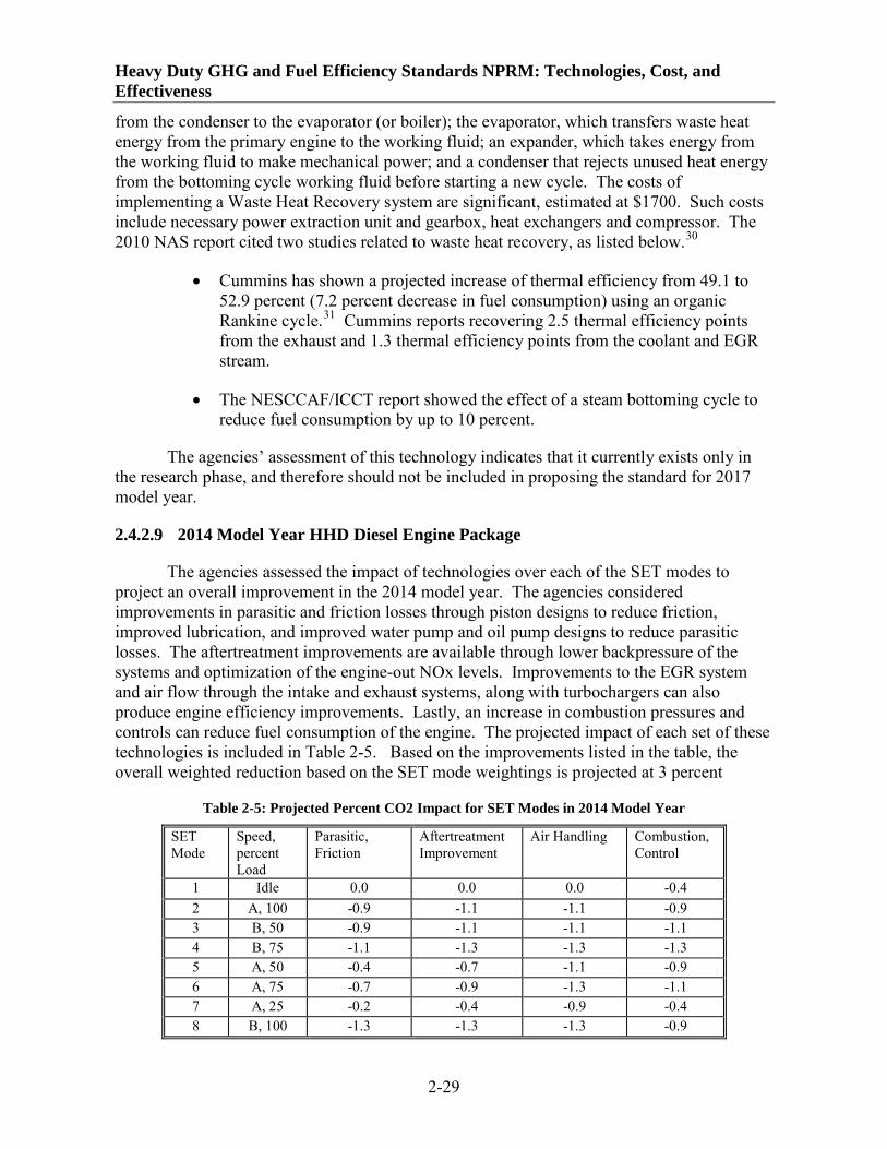
Heavy Duty GHG and Fuel Efficiency Standards NPRM: Technologies, Cost, and Effectiveness
2-29
from the condenser to the evaporator (or boiler); the evaporator, which transfers waste heat energy from the primary engine to the working fluid; an expander, which takes energy from the working fluid to make mechanical power; and a condenser that rejects unused heat energy from the bottoming cycle working fluid before starting a new cycle. The costs of implementing a Waste Heat Recovery system are significant, estimated at $1700. Such costs include necessary power extraction unit and gearbox, heat exchangers and compressor. The 2010 NAS report cited two studies related to waste heat recovery, as listed below.30
• Cummins has shown a projected increase of thermal efficiency from 49.1 to 52.9 percent (7.2 percent decrease in fuel consumption) using an organic Rankine cycle.
31
• The NESCCAF/ICCT report showed the effect of a steam bottoming cycle to reduce fuel consumption by up to 10 percent.
Cummins reports recovering 2.5 thermal efficiency points from the exhaust and 1.3 thermal efficiency points from the coolant and EGR stream.
The agencies’ assessment of this technology indicates that it currently exists only in the research phase, and therefore should not be included in proposing the standard for 2017 model year.
2.4.2.9 2014 Model Year HHD Diesel Engine Package
The agencies assessed the impact of technologies over each of the SET modes to project an overall improvement in the 2014 model year. The agencies considered improvements in parasitic and friction losses through piston designs to reduce friction, improved lubrication, and improved water pump and oil pump designs to reduce parasitic losses. The aftertreatment improvements are available through lower backpressure of the systems and optimization of the engine-out NOx levels. Improvements to the EGR system and air flow through the intake and exhaust systems, along with turbochargers can also produce engine efficiency improvements. Lastly, an increase in combustion pressures and controls can reduce fuel consumption of the engine. The projected impact of each set of these technologies is included in Table 2-5. Based on the improvements listed in the table, the overall weighted reduction based on the SET mode weightings is projected at 3 percent
Table 2-5: Projected Percent CO2 Impact for SET Modes in 2014 Model Year
SET Mode
Speed, percent Load
Parasitic, Friction
Aftertreatment Improvement
Air Handling Combustion, Control
1 Idle 0.0 0.0 0.0 -0.4 2 A, 100 -0.9 -1.1 -1.1 -0.9 3 B, 50 -0.9 -1.1 -1.1 -1.1 4 B, 75 -1.1 -1.3 -1.3 -1.3 5 A, 50 -0.4 -0.7 -1.1 -0.9 6 A, 75 -0.7 -0.9 -1.3 -1.1 7 A, 25 -0.2 -0.4 -0.9 -0.4 8 B, 100 -1.3 -1.3 -1.3 -0.9

Regulatory Impact Analysis
2-30
9 B, 25 -0.7 -0.9 -0.9 -0.4 10 C, 100 -1.7 -1.5 -1.3 -0.9 11 C, 25 -0.9 -0.9 -0.9 -0.2 12 C, 75 -1.3 -1.3 -1.1 -0.4 13 C, 50 -1.1 -1.1 -0.9 -0.7
The agencies derived the HHD diesel engine FTP technology effectiveness for the 2014 model year based on a similar approach. Using the same technologies as discussed for the HHD diesel engine SET above, the agencies project the reductions at 3 percent. It should be pointed out that individual technology improvement is not additive to each other due to the interaction of technology to technology.
The cost estimates for the complete HHD diesel engine packages are shown in Table 2-6.
Table 2-6 Technology and Package Costs for HHD Diesel Engines (2008$)
Technology 2014 2015 2016 2017 Cylinder Head $6 $6 $6 $6 Turbo efficiency $17 $17 $16 $16 EGR cooler $3 $3 $3 $3 Water pump $87 $84 $82 $79 Oil pump $4 $4 $4 $4 Fuel pump $4 $4 $4 $4 Fuel rail $10 $9 $9 $9 Fuel injector $10 $10 $10 $9 Piston $3 $3 $2 $2 Turbo-compounding (engines placed in combination tractors only) $0 $0 $0 $823 HHDD Total (vocational truck engines) $145 $140 $136 $132 HHDD Total (combination tractors) $145 $140 $136 $955
2.4.2.10 2014 Model Year LHD/MHD Diesel Engine Package
The agencies considered the same 2014 model year technology package developed for the HHD diesel engines for the LHD diesel and MHD diesel engines. The package includes parasitic and friction reduction, improved lubrication, aftertreatment improvements, EGR system and air flow improvements, and combustion pressure increase and controls to reduce fuel consumption of the engine. The agencies project that these improvements will produce a 5 percent reduction in fuel consumption and CO2
The cost estimates for the complete MHD diesel engines are shown in
.
Table 2-7. The cost estimates for the complete LHD diesel engines are shown in Table 2-8.

Heavy Duty GHG and Fuel Efficiency Standards NPRM: Technologies, Cost, and Effectiveness
2-31
Table 2-7 Technology and Package Costs for MHD Diesel Engines (2008$)
Technology 2014 2015 2016 2017 Cylinder Head $6 $6 $6 $6 Turbo efficiency $17 $17 $16 $16 EGR cooler $3 $3 $3 $3 Water pump $87 $84 $82 $79 Oil pump $4 $4 $4 $4 Fuel pump $4 $4 $4 $4 Fuel rail $10 $9 $9 $9 Fuel injector $10 $10 $10 $9 Piston $3 $3 $2 $2 Valve train friction reduction $78 $76 $73 $71 Turbo-compounding (engines placed in combination tractors only) $0 $0 $0 $823 MHDD Total (vocational truck engines) $223 $216 $210 $203 MHDD Total (combination tractors) $223 $216 $210 $1,027
Table 2-8 Technology and Package Costs for LHD Diesel Engines (2008$)
Technology 2014 2015 2016 2017 Aftertreatment improvements $111 $108 $104 $101 Cylinder Head $10 $10 $10 $9 Turbo efficiency $17 $17 $16 $16 EGR cooler $3 $3 $3 $3 Water pump $87 $84 $82 $79 Oil pump $4 $4 $4 $4 Fuel pump $4 $4 $4 $4 Fuel rail $11 $11 $11 $10 Fuel injector $14 $13 $13 $13 Piston $3 $3 $2 $2 Valve train friction reduction $104 $101 $98 $95 LHDD Total $369 $358 $348 $337
2.4.2.11 2014 Model Year Diesel Engine Standards
The agencies applied the 5 percent reduction for the LHDD/MHDD engines and the 3 percent reduction for the HHD diesel engines based on the projected technology package improvements in 2014 model year to the 2010 model year baseline performance included in Table 2-4. The results are the proposed 2014 model year standards, as shown in Table 2-9.
Table 2-9: 2014 Model Year Proposed Standards (g CO2
LHDD - FTP
/bhp-hr)
MHDD - FTP HHDD - FTP MHDD_- SET HHDD - SET 600 600 567 502 475

Regulatory Impact Analysis
2-32
2.4.2.12 2017 Model Year HHDD Engine Package
The agencies assessed the impact of technologies over each of the SET modes to project an overall improvement in the 2017 model year. The agencies considered additional improvements in the technologies included in the 2014 model year package in addition to turbocompounding. The projected impact of each set of these technologies is included in Table 2-10. Based on the improvements listed in the table, the overall weighted reduction based on the SET mode weightings is projected at 6 percent.
Costs for 2017 are shown in Table 2-6.
Table 2-10: Projected CO2
SET Mode
Improvements for SET Modes in 2017 Model Year
Speed, Percent Load
Turbo-compounding
Parasitic, Friction
Aftertreatment Improvement
Air handling
Combustion, Control
1 Idle 0.2 0.00 0.00 0.00 -0.50 2 A, 100 -4.50 -1.00 -1.25 -1.25 -1.00 3 B, 50 -2.50 -1.00 -1.25 -1.25 -1.25 4 B, 75 -4.50 -1.25 -1.50 -1.50 -1.50 5 A, 50 -1.50 -0.50 -0.75 -1.25 -1.00 6 A, 75 -4.00 -0.75 -1.00 -1.50 -1.25 7 A, 25 0.20 -0.25 -0.50 -1.00 -0.50 8 B, 100 -5.50 -1.50 -1.50 -1.50 -1.00 9 B, 25 0.30 -0.75 -1.00 -1.00 -0.50
10 C, 100 -5.00 -2.00 -1.75 -1.50 -1.00 11 C, 25 0.50 -1.00 -1.00 -1.00 -0.25 12 C, 75 -3.50 -1.50 -1.50 -1.25 -0.50 13 C, 50 -2.00 -1.25 -1.25 -1.00 -0.75
The agencies derived the HHDD FTP technology package effectiveness for the 2017 model year based on a similar approach. However, the addition of turbocompounding shows a greater effectiveness on the SET cycle than the FTP cycle because of the steady state nature and amount of time spent at higher speeds and loads during the SET. Using the same technologies as discussed for the HHDD SET above, the agencies project the reductions at 5 percent for the FTP. It is noticed that there is a small penalty on CO2 using turbocompounding at low loads from Table 2-5, since no mechanism to disengage turbocompounding and engine crankshaft is proposed in this table. This means that an introduction of a clutch to disengage turbocompound and engine whenever the turbocompounding does not provide positive work will further improve CO2
2.4.2.13 2017 Model Year LHD/MHD Diesel Engine Package
reduction. Similar to Table 2-3, individual technology in Table 2-5 is not additive to each other due to the interaction of technology to technology.
The agencies developed the 2017 model year LHD/MHD diesel engine package based on additional improvements in the technologies included in the 2014 model year package.

Heavy Duty GHG and Fuel Efficiency Standards NPRM: Technologies, Cost, and Effectiveness
2-33
The projected impact of these technologies provides an overall reduction of 9 percent over the 2010 model year baseline.
Costs for the 2017 model year are shown in Table 2-7 (MHD) and Table 2-8 (LHD).
2.4.2.14 2017 Model Year Diesel Engine Standards
The agencies applied the 8.6 percent reduction for the LHD/MHD diesel engines and the 5 percent reduction for the HHD diesel engines using the FTP and a 6.1 percent reduction for HHD diesel engines using the SET based on the projected technology package improvements in 2017 model year to the 2010 model year baseline performance included in Table 2-4. The results are the proposed 2014 model year standards, as shown in Table 2-11.
Table 2-11 2017 Model Year Proposed Standards (g CO2
LHDD - FTP /bhp-hr)
MHDD - FTP HHDD - FTP MHDD - SET HHDD - SET 576 576 555 487 460
2.5 Class 7/8 Day Cabs and Sleeper Cabs
The proposed regulatory category for Class 7 and 8 day and sleeper cabs involves seven regulatory subcategories.
Class 7 Day Cab with Low/Mid Roof
Class 7 Day Cab with High Roof
Class 8 Day Cab with Low/Mid Roof
Class 8 Day Cab with High Roof
Class 8 Sleeper Cab with Low Roof
Class 8 Sleeper Cab with Mid Roof
Class 8 Sleeper Cab with High Roof
The regulatory subcategories are being proposed to differentiate between tractor usages through using characteristics of the truck. The technologies being proposed to reduce fuel consumption and CO2 emissions from tractors can be developed for all seven subcategories. However, the typical usage pattern may limit the penetration rate of the technology. For example, aerodynamic improvements can reduce the fuel consumption and CO2 emissions of a tractor at high speeds. However, this technology could be a detriment to fuel consumption if applied to a tractor travelling at low speeds. The agencies discuss technologies, penetration rates, and costs for each regulatory subcategory in the sections below.

Regulatory Impact Analysis
2-34
2.5.1 Aerodynamics
Up to 25 percent of the fuel consumed by a line-haul truck traveling at highway speeds is used to overcome aerodynamic drag forces, making aerodynamic drag a significant contributor to a Class 7 or 8 tractor’s GHG emissions and fuel consumption.32 Because aerodynamic drag varies by the square of the vehicle speed, small changes in the tractor aerodynamics can have significant impacts on GHG emissions and fuel efficiency of that vehicle. With much of their driving at highway speed, the benefits of reduced aerodynamic drag for Class 7 or 8 tractors are significant.33
The common measure of aerodynamic efficiency is the coefficient of drag (Cd). The aerodynamic drag force (i.e., the force the vehicle must overcome due to air) is a function the Cd, the area presented to the wind (i.e., the projected area perpendicular to the direction of travel or frontal area), and the cube of the vehicle speed. Cds for today’s fleet typically range from greater than 0.80 for a “classic” body tractor to approximately 0.58 for tractors that incorporate a full package of widely, commercially available aerodynamic features.
2.5.1.1 Challenges of Tractor Aerodynamics
The aerodynamic efficiency of heavy-duty vehicles has gained increasing interest in recent years as fuel prices, competitive freight markets, and overall environmental awareness has focused owners and operators on getting as much useful work out of every gallon of diesel fuel as possible. While designers of heavy-duty vehicles and aftermarket products try to aerodynamically streamline heavy-duty vehicles, there are some challenges. Foremost is balancing the need to maximize the amount of freight that can be transported. For a tractor, this often means pulling a trailer that is as tall and as wide as motor safety laws permit, thereby presenting a large, drag-inducing area perpendicular to the wind (i.e., projected frontal area). As a result, the tractor must also present a relatively large projected frontal area to smoothly manage the flow of air along the cab and transition it to trailer. In instances where the height of the cab is not properly matched with that of trailer, aerodynamic drag can be significantly increased by creating large wakes (when the trailer is much shorter than the cab) or presenting a large non-aerodynamic surface (when the trailer is taller than the cab). Aerodynamic design must also meet practical and safety needs such as providing for physical access and visual inspections of vehicle equipment. Because weight added to the vehicle impacts its overall fuel efficiency and GHG emissions and, in some circumstances the amount of freight the vehicle can carry, aerodynamic design and devices will sacrifice some benefit to overcoming their contribution to the vehicle weight. Aerodynamic designs and devices also must balance being as light and streamlined as possible with being durable enough to withstand the rigors a working, freight vehicle encounters while traveling or loading and unloading. Durability can be a significant concern for cabs designed for specialty applications, such as “severe duty” cabs that may operate on unimproved roads. In addition, absent mandatory requirements, aerodynamic features for heavy-duty vehicles must appeal to the owners and operators. Finally, because the behavior of airflow across the cab (and cab and trailer combination) is dependent upon the entire system, it isn’t possible to make inferences about the vehicles aerodynamic performance based upon the performance of individual components. This can make it difficult to assess the benefit of adding (or

Heavy Duty GHG and Fuel Efficiency Standards NPRM: Technologies, Cost, and Effectiveness
2-35
subtracting) individual aerodynamic features and can discourage owners and operators from adopting aerodynamic technologies.
2.5.1.2 Technology to Reduce Aerodynamic Drag
Addressing aerodynamic drag in Class 7 and tractors requires considering the entire vehicle as a system to include the tractor and trailer. The overall shape can be optimized to minimize aerodynamic drag and, in fact, the tractor body must have at least a moderately aerodynamic shape (and its relatively smooth flow) to benefit from add-on aerodynamic components. Whether integrated into the shape of the tractor body or as an add-on component to a generally aerodynamic tractor, there is a wide range of technologies available for Class 7 and 8 tractors. Table 2-12 describes several of these potential aerodynamic features and components.
Table 2-12: Technologies to Address Aerodynamic Drag
LOCATION ON CAB
TECHNOLOGY TYPE
DESIGNED EFFECT
Front Bumper, grill, hood, windshield
Minimize pressure created by front of vehicle moving ambient air to make way for truck
Side Fuel tank fairings Reduce surface area perpendicular to wind, minimize opportunity to trap airflow, and smooth surface
Top Roof fairings (integrated) and wind visors (attached)
Transition air to flow smoothly over trailer and minimize surface area perpendicular to the wind (for tractor and trailer)
Rear Side extending gap reducers
Transition air to flow smoothly over trailer and reduce entrapment of air in gap between tractor and trailer
Undercarriage Underbelly treatment Manage flow of air underneath tractor to reduce eddies and smoothly transition flow to trailer
Accessories Mirrors, signal horns, exhaust
Reducing surface area perpendicular to travel and minimizing complex shapes that may induce drag
General Active air management Manage airflow by actively directing or blowing air into reduce pressure drag
General Advanced, passive air management
Manage airflow through passive aerodynamic shapes or devices that keep flow attached to the vehicle (tractor and trailer)
2.5.1.3 Aerodynamics in the Current Fleet
Aerodynamics in the Class 7 and 8 tractors fleet currently on the road ranges from trucks with few modern aerodynamic features to those that address the major areas of aerodynamic drag to tractors applying more advanced techniques. Because they operate at highway speeds less of the time, Class 7 and 8 tractors configured as day cabs (i.e., dedicated to regional routes) tend to have fewer aerodynamic features than cabs designed for line-haul applications. For tractors, it’s useful to consider aerodynamics in the current fleet as in three packages: the “classic” truck body; the “conventional” truck body; and the “SmartWay” truck body.

Regulatory Impact Analysis
2-36
“Classic” truck body: At the lower end of aerodynamic performance are tractors that have a “classic” truck body. These truck bodies prioritize looks or special duty capabilities (e.g., clearance, durability on unimproved roads, and visual access to key vehicle components) and have remained relatively unchanged since the 1970’s. Typical applications are logging, waste hauling, and some agricultural related uses. These trucks incorporate few, if any, aerodynamic features and several that detract from aerodynamics including equipment such as bug deflectors, custom sunshades, air cleaners, b-pillar exhaust stacks, additional horns, lights and mirrors may constitute a conventional vehicle.
“Conventional” truck body: The conventional, modern truck capitalizes on a generally aerodynamic shape and avoids classic features that increase drag. The conventional, modern truck body has removed extra equipment (e.g., bug deflectors, custom sunshades, additional signal horns, decorative lights), moved essential equipment out of the airflow (e.g., b-pillar exhaust stacks and air cleaners), and streamlined fixed-position, essential equipment (e.g., mirrors, steps, and safety lights).
“SmartWay” truck body: The SmartWay aerodynamic package builds off of the aerodynamic package required for a Class 8 sleeper cab high roof tractor to meet the SmartWay design specifications and represents the top aerodynamic package widely, commercially available. The SmartWay package is a fully aerodynamic truck package which has an overall streamlined shape, removes drag inducing features (i.e., those removed or moved in conventional, modern truck body), and adds components to reduce drag in the most significant areas on the tractor. This includes aerodynamic features at the front to the tractor (e.g., streamlined bumper, grill, and hood), sides (i.e., fuel tank fairings and streamlined mirrors), top (i.e., roof fairings), and rear (i.e., side extending gap reducers). Regional and line-haul applications often employ different approaches, such as removable, rooftop wind visors and fully integrated, enclosed roof fairings, respectively, based upon their intended operation.
More advanced aerodynamic features are possible and are the focus of product development, pilot and testing projects, and, in some cases, product lines that have seen limited fleet adoption. Advanced aerodynamic designs can further optimize the overall shape of the tractor and may add other advanced aerodynamic features (e.g., underbody airflow treatment, down exhaust, and lowered ride height). Some advanced aerodynamic features, including those listed above, show promise but will likely need ongoing refinement as these technologies are tailored to specific applications and payback periods are reduced. Fleets with whose line-haul operations permit are currently testing and using some advanced aerodynamic technologies.
2.5.1.4 Aerodynamic Bins
The agencies have characterized the typical aerodynamic performance (expressed as Cd) and cost for select applications. To do so, it was necessary to represent the wide variety of tractor aerodynamic shapes – which are a collection of the shapes of the multitude of component parts – by developing aerodynamic packages. These are the “classic,” “conventional,” “SmartWay,” “Advanced SmartWay,” and the “Advanced SmartWay II.”

Heavy Duty GHG and Fuel Efficiency Standards NPRM: Technologies, Cost, and Effectiveness
2-37
“Classic” aerodynamic package: As described in section 2.4.1.3, these trucks incorporate few, if any, aerodynamic features and several that detract from aerodynamics including equipment such as bug deflectors, custom sunshades, air cleaners, b-pillar exhaust stacks, additional horns, lights and mirrors may constitute a conventional vehicle. No cost for aerodynamics is assumed for the classic package.
“Conventional” package: As described in section 2.4.1.3, the conventional, modern truck capitalizes on a generally aerodynamic shape and avoids classic features that increase drag. No cost for aerodynamics is assumed for the conventional package since there has been no addition of additional body work and these moderate modifications to the tractor shape would not likely require the redesign of other components.
“SmartWay” package: Based upon the design requirements of EPA’s SmartWay Certified Tractors, this package has an overall streamlined shape, removes drag inducing features, and adds components (i.e., aerodynamic mirrors, side fairings, aerodynamic bumpers, and side extending gap reducers) to reduce drag in the most significant areas on the tractor. The SmartWay aerodynamics package does add some incremental cost above the classic and conventional packages.
“Advanced SmartWay” and “Advanced SmartWay II” packages: These packages include components similar to that found in the SmartWay package but with additional aerodynamic refinement. This can be a combination of more sophisticated shape and increased coverage of drag inducing elements. Where the Advanced SmartWay package represents a tractor using the most advanced aerodynamics available today, the Advanced SmartWay II package is designed to represent aerodynamics expected to be available in the near future. With more attention paid to aerodynamic performance than the conventional package, the Advanced SmartWay package is estimated to be slightly more expensive. As a representation of the future aerodynamics, the Advanced SmartWay II package is estimated as being 50 percent more expensive than the Advanced SmartWay package.
The agencies developed the typical coefficient of drag (Cd) values for the truck categories based on coastdown testing conducted by EPA and from literature surveys. If the Cd values found in literature were described with a frontal area, then they were converted to a Cd value that represents the frontal area being proposed by the agencies for each subcategory. In addition to the absolute values, the agencies used the results of a wind tunnel evaluation of aerodynamic components. SAE 2006-01-3456 evaluated aerodynamic components on a Class 8 high roof tractor and found that side extenders provide a Cd reduction of 0.04 and tank and cab skirts provide a Cd reduction of 0.03. 34

Regulatory Impact Analysis
2-38
Table 2-13: Tractor Cd Values
Truck Expected Bin Source Frontal Area (m2
Cd )
Class 8 Sleeper Cab High Roof International ProStar SmartWay –
Adv. SmartWay
ATDS35 9.8 0.54-0.56
NAS – Improved Tractor Adv. SmartWay
2010 NAS Report unknown 0.55-0.56
SmartWay Tractor SmartWay 2010 NAS Report unknown 0.59-0.60 Best Aero Truck SmartWay DDC Spec Manager 9.8 0.61 Full Aero SmartWay EPA PERE &
MOVES Model 9.8 0.59
Roof Deflector Conventional EPA PERE & MOVES Model
9.8 0.65
International 9200i #1 Conventional TRC 9.8 0.71 International 9200i #2 Conventional NVFEL 9.8 0.70 CE-CERT Conventional EPA PERE &
MOVES Model 9.8 0.74
No Aero Feature Classic DDC Spec Manager 9.8 0.77 Baseline Truck Classic McCallen, 1999 9.8 0.77
Class 8 Day Cab High Roof International ProStar SmartWay ATDS 9.8 0.58 Aero Features SmartWay SAE 2005-01-3512 9.8 0.61 Roof Fairing Only Conventional SAE 2005-01-3512 9.8 0.66
Class 8 Day Cab Low Roof International ProStar Conventional
- SmartWay ATDS 6.0 0.78
Based on the testing and literature information, the agencies developed the Cd value for each aerodynamic bin and tractor subcategory, as shown in Table 2-14.
Table 2-14: Coefficient of Drag Performance of the Aerodynamic Bins
Class 7 Class 8 Day Cab Day Cab Sleeper Cab Low
Roof High Roof
Low Roof High Roof
Low Roof
Mid Roof
High Roof
Aerodynamics (Cd)
Frontal Area (m2 6.0 ) 9.8 6.0 9.8 6.0 7.7 9.8 Classic 0.85 0.75 0.85 0.75 0.85 0.80 0.75 Conventional 0.80 0.68 0.80 0.68 0.80 0.75 0.68 SmartWay 0.75 0.60 0.75 0.60 0.75 0.70 0.60 Advanced SmartWay 0.70 0.55 0.70 0.55 0.70 0.65 0.55 Advanced SmartWay II
0.65 0.50 0.65 0.50 0.65 0.60 0.50
The agencies estimated the cost of the aerodynamic packages based on ICF’s price estimates.36 The agencies applied a 15 percent reduction to the prices to reflect a large

Heavy Duty GHG and Fuel Efficiency Standards NPRM: Technologies, Cost, and Effectiveness
2-39
volume discount which would be applicable to the tractor manufacturers. Although technologies such as roof fairings may already be in widespread use today, the ICF study researched retail prices that a consumer would pay for the purchase of a single item in addition to researching possible discounts based on a large volume sale, therefore this 15 percent discount was applied to reflect bulk purchases on these items. In addition, the agencies removed an RPE of 1.36 to obtain the direct manufacturer cost and then applied a low complexity ICM of 1.14 or a medium complexity ICM of 1.26 (for Advanced SmartWay II) to obtain the overall technology costs included in Table 2-15 and Table 2-16. In Table 2-17 and Table 2-18 the costs are shown including the expected penetration rates which range between 20 percent and 50 percent for most technologies shown.
Table 2-15 Estimated Aerodynamic Technology Costs for Class 7 & 8 Day Cabs for the 2014MY (2008$)
CLASS 7 DAYCAB CLASS 8 DAYCAB Low Roof High Roof Low Roof High Roof Classic $0 $0 $0 $0 Conventional $0 $0 $0 $0 SmartWay $1,079 $1,107 $1,079 $1,107 Advanced SmartWay $2,179 $2,207 $2,179 $2,207 Advanced SmartWay II $3,070 $3,111 $3,070 $3,111
Table 2-16 Estimated Aerodynamic Technology Costs for Class 8 Sleeper Cabs for the 2014My (2008$)
LOW ROOF MID ROOF HIGH ROOF Classic $0 $0 $0 Conventional $0 $0 $0 SmartWay $1,317 $1,345 $1,495 Advanced SmartWay $2,492 $2,492 $2,564 Advanced SmartWay II $3,512 $3,512 $3,613
Table 2-17 Estimated Aerodynamic Technology Costs for Class 7 & 8 Day Cabs for the 2014MY Inclusive of Penetration Rates (2008$)
CLASS 7 DAYCAB CLASS 8 DAYCAB Low Roof High Roof Low Roof High Roof SmartWay $539 $775 $647 $332 Advanced SmartWay $436 $441 $0 $883
Table 2-18 Estimated Aerodynamic Technology Costs for Class 8 Sleeper Cabs for the 2014MY Inclusive of Penetration Rates (2008$)
LOW ROOF MID ROOF HIGH ROOF SmartWay $527 $404 $1,271 Advanced SmartWay $498 $748 $256

Regulatory Impact Analysis
2-40
2.5.2 Tires
Tire rolling resistance is defined as the energy consumed by the tire per unit of distance traveled. Energy is consumed mainly by the deformation of the tires, known as hysteresis, but smaller losses are due to aerodynamic drag and other friction forces between the tire and road surface and tire and wheel rim. About 90 percent of a tire’s rolling resistance comes from hysteresis. Collectively the forces that result in energy loss from the tires are referred to as rolling resistance. The share of truck energy required to overcome rolling resistance is estimated at nearly 13 percent for Class 8 trucks37. Reducing a tire’s rolling resistance will reduce fuel consumption and lower emissions of CO2
To measure a tire’s efficiency the vertical load supported by the tire must be factored because rolling resistance is a function of the load on a tire. EPA uses a tire’s rolling resistance coefficient (RR
and other greenhouse gases. Low rolling resistance tires are commercially available from most tire manufacturers. The EPA SmartWay program identified test methods and established criteria to designate certain tires as “low rolling resistance” for use in the program’s emissions tracking system, verification program, and SmartWay vehicle specifications. Below is a discussion of EPA’s approach to quantifying tire rolling resistance and the emission reductions associated with reduced rolling resistance, and a discussion of single wide tires, retread tires, and replacement tires.
c), which is measured as the rolling resistance force over vertical load (kg/metric ton). The RRc
Beginning in 2007, EPA began designating certain Class 8 sleeper-cab configurations as Certified SmartWay Tractors. In order for a tractor to be designated as Certified SmartWay, the tractor must be equipped with verified low rolling resistance tires (either dual or single wide), among other criteria. In order to be verified as a low rolling resistance tire, a steer tire must have a RR
baseline for today’s fleet is 7.8 kg/metric ton for the steer tire and 8.2 kg/metric ton for the drive tire, based on sales weighting of the top three manufacturers based on market share. These values are based on new tires, since rolling resistance decreases as the tread wears.
c less than 6.6 kg/metric ton and a drive tire must have a RRc
Research indicates the contribution to overall vehicle fuel efficiency by tires is approximately equal to the proportion of the vehicle weight on them
less than 7.0 kg/metric ton. SmartWay-verified low rolling resistance tires are the best performing tires available based on fuel efficiency. The SmartWay program expects to decrease the maximum allowable rolling resistance coefficient by 10 percent between 2010 and 2014. As more low rolling resistance tires are sold, the baseline rolling resistance coefficient value will improve.
38
A tire’s rolling resistance is a factor considered in the design of the tire. It is a result of the tread compound material, the architect of the casing, tread design and the tire manufacturing process. Differences in rolling resistance of up to 50 percent have been
. On a fully loaded typical Class 8 long-haul truck (tractor and trailer), about 12.5 percent of the total tire energy loss attributed to rolling resistance is from the steer tires and about 42.5 percent is from the drive tires. When evaluating just the tractor, the proportionate amount of energy loss would be about 24 percent from the steer tires and 76 percent from the drive tires.

Heavy Duty GHG and Fuel Efficiency Standards NPRM: Technologies, Cost, and Effectiveness
2-41
identified for tires designed to equip the same vehicle39. It is estimated that 35 percent to 50 percent of a tire’s rolling resistance is from the tread and the other 50 to 65 percent is from the casing. Tires with increased RRc
Research and testing have shown a 5 percent reduction of rolling resistance provides a fuel consumption reduction of 1 percent while maintaining similar traction and handling characteristics. Bridgestone found a 5 percent improvement in rolling resistance will produce a 1.3 to 1.7 percent improvement in fuel economy
values are likely designed for treadwear and not fuel efficiency.
. Assuming a truck achieves 6 miles per gallon and is driven 100,000 miles annually, a 1.5 percent improvement in fuel economy results in a fuel consumption reduction of 1.48 percent, which is in line with EPA’s study. According to Bridgestone, use of a fuel-efficient tire will result in approximately a 12 percent improvement in fuel economy compared to a non-fuel efficient tire at 55 mph, and 9 percent improvement in fuel economy at 65 mph.
To further demonstrate the correlation between rolling resistance and fuel economy, Michelin modeled vehicle fuel consumption using two drive cycles and various rolling resistance values. One drive cycle incorporated several instances of stop and start that replicated driving a vehicle on a secondary road; the other drive cycle replicated driving on a highway at nearly uniform speed but with several elevation changes. Simulations were performed using a base case and for rolling resistance reductions of 10 percent and 20 percent for both the secondary roadway and highway drive cycles. The simulation modeling for the secondary road drive cycle predicts a 1.8 percent and a 3.6 percent improvement in fuel economy as a result of the 10 percent and 20 percent reduction in rolling resistance, respectively40. The simulation modeling for the highway drive cycle predicts a 2.6 percent and a 4.9 percent improvement in fuel economy as a result of the 10 percent and 20 percent reduction in rolling resistance, respectively. The modeling demonstrates less of a benefit from reduced rolling resistance when a vehicle is operated on secondary roadways. The modeling predicts an improvement in fuel economy from a reduction in rolling resistance comparable to what Bridgestone demonstrated. A 5 percent reduction in rolling resistance results in a 1 percent improvement in fuel economy.
Proper tire inflation is critical to maintaining proper stress distribution in the tire, which reduces heat loss and rolling resistance. Tires with reduced inflation pressure exhibit more sidewall bending and tread shearing, therefore, have greater rolling resistance than a tire operating at its optimal inflation pressure. Bridgestone tested the effect of inflation pressure and found a 2 percent variation in fuel consumption over a 40 psi range. Generally, a 10 psi reduction in overall tire inflation results in about a 1 percent reduction in fuel economy41
Tire rolling resistance is only one of several performance criteria that affect tire selection. The characteristics of a tire also influence durability, traction control, vehicle handling and comfort. A single performance parameter can easily be enhanced, but an optimal balance of all the criteria must be maintained. Tire design requires balancing performance, since changes in design may change different performance characteristics in opposing direction
. To achieve the intended fuel economy benefits of low rolling resistance tires, it is critical that tires are properly maintained.
42. Truck tires are most often axle-specific in relation to these different

Regulatory Impact Analysis
2-42
performance criteria43
The Center for Transportation Research at Argonne National Laboratory analyzed technology options to support energy use projections. The Center estimated the incremental cost of low rolling resistance tires of $15 - $20 per tire
. The same tire on different axles or used in different applications can a have different rolling resistance value. Any changes to a tire would generally be accompanied with additional changes to suspension tuning and/or suspension design.
. The ICF report estimated the cost of low rolling resistance steer and drive tires to be $20 and $43 per tire, respectively. The NAS panel estimated $30 per tire. EPA and NHTSA project a cost of $65 (2008$) for low rolling resistance steer tires (2 per truck) for both Class 7 and 8 tractors including a low complexity ICM of 1.14. For low rolling resistance drive tires, the agencies estimate truck-based costs of $60 (2008$) and $121(2008$) for Class 7 and 8 tractors, respectively, including a low complexity ICM of 1.14. The higher Class 8 reflects the assumption of one drive axle for Class 7 tractors and two drive axles for Class 8 tractors. All costs are considered valid for the 2014MY and time based learning would be considered appropriate for this technology.
2.5.2.1 Single Wide Tires
Low rolling resistance tires are offered for dual assembly and as single wide tires. They are typically only used on the drive axle of a tractor. A single wide tire is a larger tire with a lower profile. The common single wide sizes include: 385/65R22.5, 425/65R22.5, 445/65R22.5, 435/50R22.5 and 445/50R22.5. Generally, a single wide tire has less sidewall flexing compared to a dual assembly and therefore less hysteresis occurs. Compared to a dual tire assembly, single wide tires also produce less aerodynamic resistance or drag. Single wide tires can contribute to improving a vehicle’s fuel efficiency through design as a low rolling resistance tire and/or through vehicle weight reduction.
The use of fuel efficient single wide tires can reduce rolling resistance by 3.7 to 4.9 percent compared to the most equivalent dual tire44. An EPA study demonstrated an improvement in fuel economy of 6 percent at 55 mph on the highway, 13 percent at 65 mph on the highway and 10 percent on a suburban loop45 using single wide tires on the drive and trailer axles. EPA attributed the fuel economy improvement to the reduction in rolling resistance and vehicle weight reduction from using single wide tires. In 2008 the Department of Energy (DOE) compared the effect of different combinations of tires on the fuel efficiency of Class-8 trucks. The data collected based on field testing indicates that trucks with tractors equipped with single wide tires on the drive axle experience better fuel economy than trucks with tractors equipped with dual tires, independent of the type of tire on the trailer46
There is also a weight savings associated with single wide tires compared to dual tires. Single wide tires can reduce a tractor and trailer’s weight by as much as 1,000 lbs. when combined with aluminum wheels. Bulk haulers of gasoline and other liquids recognize the immediate advantage in carrying capacity provided by the reduction in the weight of tires and have led the transportation industry in retrofitting their tractors and trailers
. This study in particular indicated a 6.2 percent improvement in fuel economy from single wide tires.
47.

Heavy Duty GHG and Fuel Efficiency Standards NPRM: Technologies, Cost, and Effectiveness
2-43
New generation single wide tires, which were first introduced in 2000, are designed to replace a set of dual tires on the drive and/or trailer positions. They are designed to be interchangeable with the dual tires without any change to the vehicle48. If the vehicle does not have hub-piloted wheels, there may be a need to retrofit axle components. In addition to consideration of hub / bearing / axle, other axle-end components may be affected by use of single wide tires. To assure successful operation, suitable components should be fitted as recommended by the vehicle manufacturer49
Current, single wide tires are wider than earlier models and legal in all 50 states for a 5-axle, 80,000 GVW truck
.
. Single wide tires meet the “inch-width” requirements nationwide, but are restricted in certain states up to 17,500 lbs. on a single axle at 500 lbs/inch width limit, and are not allowed on single axle positions on certain double and triple combination vehicles. An inch-width law regulates the maximum load that a tire can carry as a function of the tire width. Typically single wide tires are optimized for highway operation and not city or on/off highway operation. However, newer single wide tires are being designed for better scrub resistance, which will allow an expansion of their use. The current market share of single wide tires in combination tractor applications is 5 percent and the potential market is all combination tractors.. New generation single wide tires represent an estimated 0.5 percent of the 17.5 million tires sold each year in the U.S..
The Center for Transportation Research at Argonne National Laboratory estimated incremental capital cost of single wide tires is $30 - $40 per tire. ICF estimates the incremental price of low rolling resistance tires at $20 for drive tires and $43 for steer tires.50
2.5.2.2 Replacement Tires
With 4 single wide tires replacing 8 dual tires on the drive axle of a tractor, the incremental cost would be between $120 and $160.
Original equipment (OE) tires are designed and marketed for specific applications and vehicles. Their characteristics are optimized for the specific application and vehicle. Because they are not sold as OE, replacement tires are generally designed for a variety of applications and vehicle types that require different handling characteristics. The tires marketed to the replacement tire market tend to place greater emphasis on tread wear, and therefore often have higher rolling resistance than OE tires.
The market for replacement tires is individual vehicle owners and fleet owners and not the vehicle manufacturers. Many fleets report that the cost of fuel as opposed to driver pay is its number one cost. This has resulted in a greater demand for low rolling resistance replacement tires. Both heavy-duty and medium-duty truck fleets are looking for ways to reduce operational costs.
In 2007, EPA’s SmartWay Transport Partnership introduced a means to distinguish tires based on their rolling resistance. Since 2007 the number of low rolling resistance tires available to vehicle owners and vehicle fleets has increased greatly, which is an indicator of an increase in demand. EPA expects this trend to continue. In addition, effective January 1, 2010, California Air Resource Board requires that all tractor-trailers hauling dry van trailers on any California road be equipped with SmartWay verified low rolling resistance tires; other

Regulatory Impact Analysis
2-44
states may adopt this requirement. EPA expects this requirement will drive the demand for low rolling resistance tires even further.
2.5.2.3 Retreaded Tires
The tread life of a tire is a measure of durability and some tires are designed specifically for greater durability. Commercial truck tires are designed to be retreaded, a process in which a new tread compound is adhered to the tire casing. The original tread of a tire will last anywhere from 100,000 miles to over 300,000 miles, depending on vehicle operation, original tread depth, tire axle position, and proper tire maintenance. Retreading can extend the tire’s useful life by 100,000 miles or more.51 In 2005, the Tire Industry Association estimated that approximately 17.6 million retreaded truck tires were sold in North America52
To maintain the quality of the casing and increase the likelihood of retreading, a tire should be retreaded before the tread depth is reduced to its legal limit. At any time, a steer tire must have a tread depth of at least 4/32 of an inch and a drive tire must have a tread depth of at least 2/32 of an inch (49 CFR. § 393.75). To protect the casing, a steer tire is generally retreaded once the tread is worn down to 6/32 of an inch and a drive tire is retreaded once the tread is worn down to 8/32 of an inch.
.
53
Both the casing and the tread contribute to a tire’s rolling resistance. It is estimated that 35 percent to 50 percent of a tire’s rolling resistance is the result of the tread.
Tires used on Class 8 vehicles are retreaded as many as three times.
Differences in drive tire rolling resistance of up to 50 percent for the same casing with various tread compounds have been demonstrated. For example, a fuel efficient tread compound (as defined by the manufacturer) was added to two different casings resulting in an average increase in rolling resistance of 48 percent. When a nonfuel efficient tread compound (also defined by the manufacturer) was added to the same casings, the rolling resistance increased by 125 percent on average. This characterizes the effect of the tread on the rolling resistance of a tire.
Because tires can be retreaded multiple times, changes in the casing due to wear, damage and material aging may impact rolling resistance to a greater degree than would occur in an original tire. Additionally, as evidenced above, if a tread compound different than the original tread is used, a retreaded tire can have higher or lower rolling resistance than the original tire.
There is a cost savings associated with retread tires. A new retread costs between $150 and $200, compared to a new tire which costs typically around $400. Since retreads are not typically used on the steer axle position, this represents a savings of $1,600 to $2,000 per tractor.
2.5.2.4 Tire Rolling Resistance
The agencies are projecting the following tire rolling resistance performance for setting the proposed tractor standards, as shown in Table 2-19.

Heavy Duty GHG and Fuel Efficiency Standards NPRM: Technologies, Cost, and Effectiveness
2-45
Table 2-19 Tire Rolling Resistance
Class 7 Class 8 Day Cab Day Cab Sleeper Cab Low/
Mid Roof
High Roof
Low/Mid Roof
High Roof
Low Roof
Mid Roof
High Roof
Steer Tires (Crr kg/metric ton) Baseline 7.8 7.8 7.8 7.8 7.8 7.8 7.8 SmartWay 6.6 6.6 6.6 6.6 6.6 6.6 6.6 Advanced SmartWay 5.7 5.7 5.7 5.7 5.7 5.7 5.7
Drive Tires (Crr kg/metric ton) Baseline 8.2 8.2 8.2 8.2 8.2 8.2 8.2 SmartWay 7.0 7.0 7.0 7.0 7.0 7.0 7.0 Advanced SmartWay 6.0 6.0 6.0 6.0 6.0 6.0 6.0
2.5.3 Weight Reduction
Mass reduction encompasses a variety of techniques ranging from improved design and better component integration to application of lighter and higher-strength materials. Mass reduction can be further compounded by reductions in engine power and ancillary systems (transmission, steering, brakes, suspension, etc.). Although common on light-duty passenger vehicles for fuel economy and performance increases, mass reduction on heavy-duty vehicles is more complex due to the size and duty cycle of the vehicles.
Reducing a vehicle’s mass decreases fuel consumption and GHG output by reducing the energy demand needed to overcome forces resisting motion, and rolling resistance. Passenger vehicle manufacturers employ a systematic approach to mass reduction, where the net mass reduction is the addition of a direct component or system mass reduction plus the additional mass reduction taken from indirect ancillary systems and components, effectively compounding or obtaining a secondary mass reduction from a primary mass reduction. For example, use of a smaller, lighter engine with lower torque-output subsequently allows the use of a smaller, lighter-weight transmission and drive line components. Likewise, the compounded weight reductions of the body, engine and drivetrain reduce stresses on the suspension components, steering components, wheels, tires and brakes, allowing further reductions in the mass of these subsystems. The reductions in unsprung masses such as brakes, control arms, wheels and tires further reduce stresses in the suspension mounting points. This produces a compounding effect of ripple effect of possible mass reductions.
A fully loaded tractor-trailer combination can weigh up to 80,000 pounds. Reduction in overall vehicle weight could enable an increase in freight delivered on a ton-mile basis. Practically, this enables more freight to be delivered per truck and improves freight transportation efficiency. In certain applications, heavy trucks are weight-limited (i.e. bulk cargo carriers), and reduced tractor and trailer weight allows direct increases in the quantity of material that can be carried.
Mass reduction can be accomplished by proven methods such as:

Regulatory Impact Analysis
2-46
• Smart Design: Computer aided engineering (CAE) tools can be used to better optimize load paths within structures by reducing stresses and bending moments applied to structures. This allows better optimization of the sectional thicknesses of structural components to reduce mass while maintaining or improving the function of the component. Smart designs also integrate separate parts in a manner that reduces mass by combining functions or the reduced use of separate fasteners.
• Material Substitution: Substitution of lower density and/or higher strength materials into a design in a manner that preserves or improves the function of the component. This includes substitution of high-strength steels, aluminum, magnesium or composite materials for components currently fabricated from mild steel. Mass reduction through material substitution is currently broadly applied across in both light and heavy-duty applications in all vehicle subsystems such as aluminum engine block, aluminum transmission housing, high-strength steel body structure, etc.
• Reduced Powertrain Requirements: Reducing vehicle weight sufficiently can allows for the use of a smaller, lighter and more efficient engine while maintaining or increasing work or cargo requirements. The subsequent reduced rotating mass (e.g., transmission, driveshafts/halfshafts, wheels and tires) via weight and/or size reduction of components are made possible by reduced torque output requirements.
Reduced mass in heavy-duty vehicles can benefit fuel efficiency and CO2
Mass reduction can be achieved by making components with lighter materials (high strength steel, aluminum, composites) or by eliminating components from the truck. A common component-elimination example is to use single wide tires and aluminum rims to replace traditional dual tires and rims, eliminating eight steel rims and eight tires. Although many gains have been made to reduce truck mass, many of the features being added to modern trucks to benefit fuel economy, such as additional aerodynamic features or idle reduction systems, have the effect of increasing truck weight causing mass to stay relatively constant. Material and manufacturing technologies can also play a significant role in vehicle safety by reducing vehicle weight, and in the improved performance of vehicle passive and active safety systems. Although new vehicle systems, such as hybrid power trains, fuel cells and auxiliary power will present complex packaging and weight issues, this will further increase the need for reductions in the weight of the body, chassis, and power train components in order to maintain vehicle functionality.
emissions in two ways. If a truck is running at its gross vehicle weight limit with high density freight, more freight can be carried on each trip, increasing the trucks ton-miles per gallon. If the truck is carrying lower density freight and is below the GVW limit, the total vehicle mass is decreased, reducing rolling resistance and the power required to accelerate or climb grades.
EPA’s SmartWay transport web page discusses how the truck fuel consumption increases with the weight of the vehicle. Many truck components are typically made of heavier material, such as steel. Heavier trucks require more fuel to accelerate and to climb hills, and may reduce the amount of cargo that can be carried.54 Every 10 percent drop in truck weight reduces fuel use about 5 percent. Generally, an empty truck makes up about one-third of the total weight of the truck. Using aluminum, metal alloys, metal matrix composites,

Heavy Duty GHG and Fuel Efficiency Standards NPRM: Technologies, Cost, and Effectiveness
2-47
and other lightweight components where appropriate can reduce empty truck weight (known as “tare weight”), improve fuel efficiency, and reduce greenhouse gas emissions. As an example, trimming 3,000 pounds from a heavy truck (about 4 percent of its loaded weight) with lighter-weight components could improve fuel economy by up to 3 percent and trucks that employ more weight saving options would save more. In addition, in weight-sensitive applications, lightweight components can allow more cargo and increased productivity. Another report by the National Commission on Energy Policy estimates that a fuel economy gain of 5.0 percent on certain applications could be achieved by vehicle mass reduction further illustrating the fuel economy gains possible on heavy-duty applications55
In support of the overall goal to cost-effectively enable trucks and other heavy vehicles to be more energy efficient and to use alternative fuels while reducing emissions, the 21st Century Truck Partnership seeks to reduce parasitic energy losses due to the weight of heavy vehicles without reducing vehicle functionality, durability, reliability, or safety, and to do so cost-effectively. Aggressive weight reduction goals vary according to the weight class of the vehicle with targets between 10 and 33 percent. The weight targets for each vehicle class depend on the performance requirements and duty cycle. It is important to note that materials or technologies developed for a particular vehicle class are not necessarily limited to that class. For example, materials developed for lightweight frames for pickup trucks, vans, or SUVs will eventually be used in Class 3-5 vehicles, and materials developed to meet the demanding performance requirements for Class 7 and 8 trucks will find application in smaller vehicles. Weight reduction must not in any way sacrifice the durability, reliability, and performance of the vehicle. Attaining these goals by reducing inertial loading will yield substantial benefits such as increased fuel efficiency with concomitant reductions in emissions, increased available payload capacity for some vehicles, reduced rolling resistance, and optimized safety structures and aerodynamic drag reduction systems.
. A third report, estimated potential reductions in modal GHG emissions are 4.6 percent, however also states current light-weight materials are costly and are application and vehicle specific with further research and development for advanced materials are needed.
A 2009 NESCAFF report evaluated the potential to reduce fuel consumption and CO2
emissions by reducing weight from the baseline weight of 80,000 pounds. For the purpose of this calculation, the weight reduction could come either from carrying lighter freight or from a reduction in the empty weight of the truck. If the vehicle mass is reduced to 65,000 pounds, the fuel economy improves to 5.9 MPG from 5.4 MPG. The fuel savings and CO2
Argonne has also attempted to simulate the effect of mass reduction on the fuel economy of heavy trucks through the National Renewable Energy Laboratory’s Advanced Vehicle Simulator Model, ADVISOR. The Argonne simulations relied on a few driving schedules developed by the West Virginia University (WVU) because there are no established driving schedules for heavy trucks,. While simulating a Class 8 truck on the WVU Intercity Driving Schedule, a fuel economy gain of 0.6 percent was observed for each 1 percent mass reduction from 65,000 lb to 58,000 lb
reduction on the baseline vehicle amount to about 0.5 percent per 1,000 pounds of mass reduction. This result suggests that efforts to reduce the empty vehicle mass will have only a modest benefit on fuel economy, for long haul routes.
56. The maximum speed during the simulation was 61

Regulatory Impact Analysis
2-48
mph, and the average running speed (excluding stops) was 37.5 mph although most intercity Class 8 trucks average a much higher speed than 37.5 mph. Argonne assumed a 0.66 percent increase in fuel economy for each 1 percent weight reduction and total possible estimated fuel economy increases of 5–10 percent. While simulating a Class 6 truck on a WVU Suburban Driving Schedule, a fuel economy gain of 0.48 percent was observed for each 1 percent mass reduction from 22,600 lb to 21,800 lb. The maximum speed during the simulation was 44.8 mph, and the average running speed was 21.5 mph. The potential fuel economy gains for medium trucks, both heavy- and light-, were capped at 5 percent since they are less likely to be weight or volume limited, and so the use of expensive lightweight material would not be cost-effective.
The principal barriers to overcome in reducing the weight of heavy vehicles are associated with the cost of lightweight materials, the difficulties in forming and manufacturing lightweight materials and structures, the cost of tooling for use in the manufacture of relatively low-volume vehicles (when compared to automotive production volumes), and ultimately, the extreme durability requirements of heavy vehicles. While light-duty vehicles may have a life span requirement of several hundred thousand miles, typical heavy-duty commercial vehicles must last over 1 million miles with minimum maintenance, and often are used in secondary applications for many more years. This requires high strength, lightweight materials that provide resistance to fatigue, corrosion, and can be economically repaired. Additionally, because of the limited production volumes and the high levels of customization in the heavy-duty market, tooling and manufacturing technologies that are used by the automotive industry are often uneconomical for heavy vehicle manufacturers. Lightweight materials such as aluminum, titanium and carbon fiber composites provide the opportunity for significant weight reductions, but their material cost and difficult forming and manufacturing requirements make it difficult for them to compete with low-cost steels. In addition, although mass reduction is currently occurring on both vocational and line haul trucks, the addition of other systems for fuel economy, performance or comfort increases the truck mass offsetting the mass reduction that has already occurred, thus is not captured in the overall truck mass measurement.
Most truck manufacturers offer lightweight tractor models that are 1,000 or more pounds lighter than comparable models. Lighter-weight models combine different weight-saving options that may include: 57
• Cast aluminum alloy wheels can save 40 pounds each for total savings of 400 pounds
• Aluminum axle hubs can save over 120 pounds compared to ductile iron or steel • Centrifuse brake drums can save nearly 100 pounds compared to standard brake drums • Aluminum clutch housing can save 50 pounds compared to iron clutch housing • Composite front axle leaf springs can save 70 pounds compared to steel springs • Aluminum cab frames can save hundreds of pounds compared to standard steel frames • Downsizing to a smaller, lighter-weight engine can save over 700 pounds58
2.5.3.1 Derivation of Weight Technology Packages
The agencies see many opportunities for weight reduction in tractors. However, the empty curb weight of tractors varies significantly today. Items as common as fuel tanks can vary between 50 and 300 gallons each for a given truck model. Information provided by truck

Heavy Duty GHG and Fuel Efficiency Standards NPRM: Technologies, Cost, and Effectiveness
2-49
manufacturers indicates that there may be as much as a 5,000 to 17,000 pound difference in curb weight between the lightest and heaviest tractors within a regulatory subcategory (such as Class 8 sleeper cab with a high roof). Because there is such a large variation in the baseline weight among trucks that perform roughly similar functions with roughly similar configurations, there is not an effective way to quantify the exact CO2 and fuel consumption benefit of mass reduction using GEM because of the difficulty in establishing a baseline. However, if the weight reduction is limited to tires and wheels, then both the baseline and weight differentials for these are readily quantifiable and well-understood. Therefore, the agencies are proposing that the mass reduction that would be simulated be limited only to reductions in wheel and tire weight. The agencies still encourage each OEM to reduce tractor curb weight in as many other ways as possible, which would reduce emission and fuel consumption independent of the degree to which such improvements are recognized for fuel consumption and CO2
EPA and NHTSA are proposing to specify the baseline vehicle weight for each regulatory category (including the tires and wheels), but allow manufacturers to quantify weight reductions based on the wheel material selection and single wide versus dual tires per
compliance purposes. In the context of this heavy-duty vehicle program with only changes to tires and wheels, the agencies do not foresee any related impact on safety.
Table 2-20. The agencies assume the baseline wheel and tire configuration contains dual tires with steel wheels. The proposed weight reduction due to the wheels and tires would be reflected in the payload tons by increasing the specified payload by the weight reduction amount discounted by two thirds to recognize that approximately one third of the truck miles are travelled at maximum payload.
Table 2-20: Proposed Weight Reductions
Weight Reduction (lb) Single Wide Tire (per tire) 57 High strength steel dual wheel (per wheel) 8 Aluminum dual wheel (per wheel) 21 Light weight aluminum dual wheel (per wheel) 30 Steel single wide wheel (per wheel) 27 Aluminum single wide wheel (per wheel) 82 Light weight aluminum single wide wheel (per wheel) 90
The agencies have estimated costs for these technologies. Those costs are shown in Table 2-21. The costs shown include a low complexity ICM of 1.14 and time based learning would be considered appropriate for these technologies.
Table 2-21 Estimated Weight Reduction Technology Costs for Class 7 & 8 Tractors for the 2014MY (2008$)
CLASS 7 TRACTORS CLASS 8 TRACTORS Single Wide Tire (per tire) $322 $644 Aluminum Steer Wheel $523 $523 Aluminum Wheels - dual $1,569 $2,615 Aluminum Wheel – Single wide $627 $1,254

Regulatory Impact Analysis
2-50
2.5.4 Extended Idle
Class 8 heavy-duty diesel truck extended engine idling wastes significant amounts of fuel in the United States. Department of Transportation regulations require a certain amount of rest for a corresponding period of driving hours. Extended idle occurs when Class 8 long haul drivers rest in the sleeper/cab compartment during rest periods as drivers find it more convenient and economical to rest in the truck cab itself. In many cases it is the only option available. During this rest period a driver will idle the truck in order to provide heating or cooling or run on-board appliances. During rest periods the truck’s main propulsion engine is running but not engaged in gear and it remains in a stationary position. In some cases the engine can idle in excess of 10 hours. During this period of time, fuel consumption will generally average 0.8 gallons per hour. Average overnight fuel usage would exceed 8 gallons in this example. When multiplied by the number of long haul trucks without idle control technology that operate on national highways on a daily basis the number of gallons consumed by extended idling would exceed 3 million gallons per day. Fortunately, a number of alternatives (idling reduction technologies) are available to alleviate this situation.
2.5.4.1 Idle Control Technologies
Idle reduction technologies in general utilize an alternative energy source in place of operating the main engine. By using these devices the truck driver can obtain needed power for services and appliances without running the engine. A number of these devices attach to the truck providing heat, air conditioning, or electrical power for microwave oven, televisions, etc.
The idle control technologies available today include the following:59
• Auxiliary Power Unit (APU) which powers the truck’s heating, cooling, and electrical system. The fuel use of an APU is typically 0.2 gallons per hour
• Fuel Operated Heater (FOH) provides heating services to the truck through small diesel fired heaters. The fuel use is typically 0.04 gallons per hour.
• Battery Air Conditioning Systems (BAC) provides cooling to the truck.
• Thermal Storage Systems provide cooling to trucks.
Another alternative involves electrified parking spaces (EPS) with or without modification to the truck. An EPS system operates independently of the truck’s engine and allows the truck engine to be turned off as the EPS system supplies heating, cooling, and electrical power. The EPS system provides off-board electrical power to operate either:
1. A single system electrification requires no on-board equipment by providing an independent heating, cooling, and electrical power system, or
Heavy Duty GHG and Fuel Efficiency Standards NPRM: Technologies, Cost, and Effectiveness
2-51
2. A dual system which allows driver to plug in on-board equipment
In the first case power is provided to stationary equipment that is temporarily attached to the truck. In the second, the truck is modified to accept power from the electrical grid to operate on board truck equipment. The retail price of idle reduction systems varies depending on the level of sophistication, for example, on-board technologies such as APUs can retail for over $7,000 while options such as EPS require negligible up-front costs for equipment for the truck itself, but will accrue fees with usage.
2.5.4.2 CO2
CO
g/ton-mile Idle Reduction Benefit
2 emissions during extended idling are a significant contributor to Class 8 sleeper cabs. The federal test procedure does evaluate idle emissions as part of the drive cycle and related emissions measurement. However, long duration extended idle emissions are not fully represented during the prescribed test cycle. Consequently, there is an opportunity to recognize the CO2 reductions attributed to idle control systems by employing a credit mechanism for manufacturers who provide for idle control devices in the original truck/ tractor build or in the case of EPS provide a pre-purchase plan for EPS facility use and install all necessary equipment on the tractor. The credit would allow truck manufacturers additional flexibility in product design and performance capabilities as the CO2
Truck owners can obtain verified idle reduction technologies on a new truck at the time of purchase from the manufacturer or retrofit with verified technology after purchase provided a retrofit agreement is in place prior to introduction into commerce. For a manufacturer to qualify for the reduction, the agencies are proposing that a truck have an automatic engine shut-off system that shuts off the engine after five minutes of idling when it is in a parked position. This approach allows for operational strategies such as electrified parking spaces, team drivers, and overnights spent in hotels to achieve and idle reduction while still being tied back to a verifiable technology (i.e., engine shutoff).
requirements are put in place.
Idle reduction credits would be based on the GHG emission and fuel consumption reduction from the technology when compared to main engine idling, as shown in Table 2-22. The main engine consumes approximately 0.8 gallons per hour during idling.60 Using a factor of 10,180 grams of CO2 per gallon of diesel fuel, the CO2 emissions from the main engine at idle is 8,144 g per hour. The agencies assumed the average Class 8 sleeper cab spends 1,800 hours in extended idle per year to determine the idling emissions per year.61 The agencies then assumed the average Class 8 sleeper cab travels 125,000 miles per year (500 miles per day and 250 days per year) and carries 19 tons of payload (the standardized payload proposed for Class 8 tractors) to calculate the baseline emissions as 6.2 grams of CO2
The engine used to power the APU consumes an approximately 0.2 gallons of diesel fuel per hour.
per ton-mile.
62 The CO2 emissions from the APU equate to 1.5 grams per ton-mile. Therefore, the agencies are proposing an idle reduction credit 5 g CO2 per ton-mile which represents the difference in emissions between the main engine idling and idling with an APU. Credits as proposed are based on the requirement that all Class 8 sleeper cabs shall be

Regulatory Impact Analysis
2-52
equipped with and automatic engine shut-off. The credit reflects a technology’s fuel consumption in conjunction with a shut-off.
Table 2-22: Idle Credit Calculation
2.5.5 Vehicle Speed Limiters
As discussed above, the power required to move a vehicle increases as the vehicle speed increases. Travelling at lower speeds provides additional efficiency to the vehicle performance. Most vehicles today have the ability to electronically control the maximum vehicle speed through the engine controller. This feature is used today by fleets and owners to provide increased safety and fuel economy. Currently, these features are able to be changed by the owner and/or dealer.
The impact of this feature is dependent on the difference between the governed speed and the speed that would have been travelled, which is dependent on road type, state speed limits, traffic congestion, and other factors. EPA will be assessing the benefit of a vehicle speed limiter by reducing the maximum drive cycle speed on the 65 mph Cruise mode of the cycle. The maximum speed of the drive cycle is 65 mph, therefore any vehicle speed limit with a setting greater than this will show no benefit for regulations, but may still show benefit in the real world in states where the interstate truck speed limit is greater than the national average of 65.5 mph.
The benefits of this simple technology are widely recognized. The American Trucking Association (ATA) developed six recommendations to reduce carbon emissions from trucks in the United States. Their first recommendation is to enact a national truck speed limit of 65 mph and require that trucks manufactured after 1992 have speed governors set at not greater than 65 mph.63 The SmartWay program includes speed management as one of their key Clean Freight Strategies and provides information to the public regarding the benefit of lower highway speeds.64
Some countries have enacted regulations to reduce truck speeds. For example, the United Kingdom introduced regulations in 2005 which require new trucks used for goods movement to have a vehicle speed limiter not to exceed 90 kph (56 mph).
65
The Canadian Provinces of Ontario and Quebec developed regulations which took effect in January 2009
Idle Fuel Consumption
(gal/hour)
Idle CO2 emissions per hour
Idle Hours
per Year
Idle CO2 Emission per year (grams)
Miles Per
Year
Payload (tons)
GHG Emissions
due to Idling (g/ton-mile)
GHG Reduction
(g/ton-mile)
Fuel Consumption
Reduction (gal/100 ton-
mile)
Baseline 0.8 8,144 1,800 14,659,200 125,000 19 6.2
Idle Reduction Technology
0.2 2,036 1,800 3,664,800 125,000 19 1.5 5 0.05

Heavy Duty GHG and Fuel Efficiency Standards NPRM: Technologies, Cost, and Effectiveness
2-53
that requires on-highway commercial heavy-duty trucks to have speed limiters which limit the truck’s speed to 105 km/h.66
Many truck fleets consider speed limiter application a good business practice in their operations. A Canadian assessment of heavy-duty truck speed limiters estimated that 60 percent of heavy truck fleets in North America use speed limiters.
67 Con Way Freight, Con Way Truckload, and Wal-Mart currently govern the speeds of their fleets between 62 and 65 mph.68
A potential disbenefit of this technology is the additional time required for goods movement, or loss of productivity. The elasticity between speed reduction and productivity loss has not been well defined in industry. The Canadian assessment of speed limiters found that the fuel savings due to the lower operating speeds outweigh any productivity losses. A general consensus among the OEMs is that a one percent decrease in speed might lower productivity by approximately 0.2 percent.
69
There is no additional capital cost associated with a vehicle speed limiter. There are no hardware requirements for this feature, only software control strategies. Nearly all heavy-duty engines today are electronically controlled and are capable of being programmed for a maximum vehicle speed. The only new requirement for truck manufacturers is to offer a vehicle speed limiter which is protected from tampering and cannot be changed by the fleet or truck owner. This technology is required to be used for the full useful life of the vehicle to obtain the GHG emissions reduction.
The vehicle speed limiter is applicable to all truck classes which operate at high speeds. However, due to the structure of the first phase of the Heavy-Duty truck program, it is only applicable to the Class 7-8 tractors. The benefits of the vehicle speed limiter are assessed through the use of alternate High Speed Cruise cycles. The baseline cycle contains a constant 65 mph cruise.
2.5.6 Automated Manual Transmission
Most heavy-duty trucks use manual transmissions with 8 to 18 ratios available. The most common transmissions for line haul applications have 10 ratios with an overdrive top gear. Torque-converter automatic transmissions, similar to those used in passenger cars, are used in some stop/go truck applications but are more expensive do not have an efficiency advantage in line-haul applications. Automated manual transmissions have been available on the market for over 10 years now and are increasing in market share. Automated manuals have a computer to decide when to shift and use pneumatic or hydraulic mechanisms to actuate the clutch and hidden shift levers. An automated manual can shift as quickly as the best driver, and the shift schedule can be tailored to match the characteristics of the engine and vehicle. This reduces variability of fuel consumption and CO2 emissions between drivers, with all drivers achieving results closer to those of the best drivers. In application, there would be a fuel economy improvement proportional to the number of non-fuel-conscious drivers in a fleet. [Reducing Heavy-Duty Long Haul Combination Truck Fuel Consumption and CO2 Emissions, NESCCAF/ICCT Final Report, October, 2009]

Regulatory Impact Analysis
2-54
2.5.7 Class 7-8 Tractor Baseline Assessment
The agencies developed the baseline tractor for each subcategory to represent an average 2010 model year tractor. The approach taken by the agencies was to define the individual inputs to GEM. For example, the agencies evaluated the industry’s tractor offerings and conclude that the average tractor contains a generally aerodynamic shape (such as roof fairings) and avoid classic features such as exhaust stacks at the b-pillar which increase drag. The agencies consider a baseline truck as having “conventional” aerodynamics. The baseline rolling resistance coefficient for today’s fleet is 7.8 kg/metric ton for the steer tire and 8.2 kg/metric ton for the drive tire, based on sales weighting of the top three manufacturers based on market share.70
Table 2-23 Class 7 and 9 Baseline Attributes
However, today there is a large spread in aerodynamics in the new tractor fleet. Trucks are sold that reflect classic styling, or are sold with conventional or SmartWay aerodynamic packages.
Class 7 Class 8 Day Cab Day Cab Sleeper Cab Low/Mid
Roof High Roof Low/Mid
Roof High Roof Low Roof Mid Roof High Roof
Aerodynamics (Cd)
Frontal Area (m2 6.0 ) 9.8 6.0 9.8 6.0 7.7 9.8 Baseline 0.81 0.69 0.81 0.69 0.81 0.76 0.69
Steer Tires (Crr kg/metric ton) Baseline 7.8 7.8 7.8 7.8 7.8 7.8 7.8
Drive Tires (Crr kg/metric ton) Baseline 8.2 8.2 8.2 8.2 8.2 8.2 8.2
Weight Reduction (lbs.) Baseline 0 0 0 0 0 0 0
Extended Idle Reduction (gram CO2
Baseline /ton-mile reduction)
N/A N/A N/A N/A 0 0 0 Vehicle Speed Limiter
Baseline -- -- -- -- -- -- --
2.5.8 Class 7-8 Tractor Standards Derivation
EPA and NHTSA project that CO2 emissions and fuel consumption reductions can be achieved through the increased penetration of aerodynamic technologies, low rolling resistance tires, weight reduction, extended idle reduction technologies, and vehicle speed limiters. The agencies believe that hybrid powertrains in line haul applications will not be cost effective in the time frame of the rule. The agencies also are proposing to not include drivetrain technologies in the standard setting process, as discussed in Section II, instead are choosing to allow the continuation of the current truck specifying process that is working well today.

Heavy Duty GHG and Fuel Efficiency Standards NPRM: Technologies, Cost, and Effectiveness
2-55
The agencies started with a goal of essentially forcing SmartWay technologies (aerodynamics, tires, and extended idle) into 100 percent of Class 7 and Class 8 tractors. However, as discussed below, the agencies realize that there are some restrictions which prevent 100 percent penetration. Therefore, the agencies took the approach of evaluating each technology and proposing what we deem as the maximum feasible penetration into each tractor regulatory category. The next sections describe the effectiveness of the individual technologies, the costs of the technologies, the proposed penetration rates of the technologies into the regulatory categories, and finally the derivation of the proposed standards.
2.5.8.1 Technology Effectiveness
The agencies’ assessment of the proposed technology effectiveness was developed through the use of the GEM Model in coordination with chassis testing of three SmartWay certified Class 8 sleeper cabs. The agencies are projecting the following tire rolling resistance performance for setting the proposed tractor standards, as shows in Table 2-19. Table 2-24 describes the proposed model inputs for the range of Class 7 and 8 tractor technologies.
Table 2-24: GEM Inputs
Class 7 Class 8 Day Cab Day Cab Sleeper Cab Low Roof High Roof Low Roof High Roof Low Roof Mid Roof High Roof
Aerodynamics (Cd)
Frontal Area (m2 6.0 ) 9.8 6.0 9.8 6.0 7.7 9.8 Classic 0.85 0.75 0.85 0.75 0.85 0.80 0.75 Conventional 0.80 0.68 0.80 0.68 0.80 0.75 0.68 SmartWay 0.75 0.60 0.75 0.60 0.75 0.70 0.60 Advanced SmartWay 0.70 0.55 0.70 0.55 0.70 0.65 0.55 Advanced SmartWay II 0.65 0.50 0.65 0.50 0.65 0.60 0.50
Steer Tires (Crr kg/metric ton) Baseline 7.8 7.8 7.8 7.8 7.8 7.8 7.8 SmartWay 6.6 6.6 6.6 6.6 6.6 6.6 6.6 Advanced SmartWay 5.7 5.7 5.7 5.7 5.7 5.7 5.7
Drive Tires (Crr kg/metric ton) Baseline 8.2 8.2 8.2 8.2 8.2 8.2 8.2 SmartWay 7.0 7.0 7.0 7.0 7.0 7.0 7.0 Advanced SmartWay 6.0 6.0 6.0 6.0 6.0 6.0 6.0
Weight Reduction (lbs.) Control 400 400 400 400 400 400 400
Extended Idle Reduction (gram CO2
Control /ton-mile reduction)
N/A N/A N/A N/A 5 5 5 Vehicle Speed Limiter
Control N/A N/A N/A N/A N/A N/A N/A

Regulatory Impact Analysis
2-56
2.5.8.2 Class 7-8 Tractor Application Rates
Vehicle manufacturers often introduce major product changes together, as a package. In this manner the manufacturers can optimize their available resources, including engineering, development, manufacturing and marketing activities to create a product with multiple new features. In addition, manufacturers recognize that an engine and truck will need to remain competitive over its intended life and meet future regulatory requirements. In some limited cases, manufacturers may implement an individual technology outside of a vehicle’s redesign cycle. In following with these industry practices, the agencies have created a set of vehicle technology packages for each regulatory subcategory.
With respect to the level of technology required to meet the standards, NHTSA and EPA established technology application caps. The first type of cap was established based on the application of common fuel consumption and CO2
The impact of aerodynamics on a truck’s efficiency increases with vehicle speed. Therefore, the usage pattern of the truck will determine the benefit of various aerodynamic technologies. Sleeper cabs are often used in line haul applications and drive the majority of their miles on the highway travelling at speeds greater than 55 mph. The industry has focused aerodynamic technology development, including SmartWay certified tractors, on these types of trucks. Therefore the agencies are proposing the most aggressive aerodynamic technology penetration in this regulatory subcategory. All of the major manufacturers today offer at least one truck model that is SmartWay certified. The National Academy of Sciences report on heavy-duty truck found that manufacturers indicated that aerodynamic improvements which yield 3 to 4 percent fuel consumption reduction or 6 to 8 percent reduction in Cd values, beyond technologies used in today’s SmartWay trucks are achievable.
emission reduction technologies into the different types of tractors. For example, idle reduction technologies are limited to Class 8 sleeper cabs using the assumption that day cabs are not used for overnight hoteling. A second type of constraint was applied to most other technologies and limited their penetration based on factors such as market demands.
71
The aerodynamic penetration for the other tractor regulatory subcategories is less aggressive than for the Class 8 sleeper cab high roof. The agencies acknowledge that there are truck applications which require on/off-road capability and other truck functions which restrict the type of aerodynamic equipment applicable. We also recognize that these types of trucks spend less time at highway speeds where aerodynamics have the greatest benefit. The 2002 Vehicle Inventory and Use Survey (VIUS) data ranks trucks by major use.
EPA and NHTSA are proposing that the aerodynamic penetration rate for Class 8 sleeper cab high roof cabs to consist of 20 percent of advanced SmartWay, 70 percent SmartWay, and 10 percent conventional. The small percentage of conventional truck aerodynamics is for applications such as refuse haulers which spend a portion of their time off-road at the land fill. Features such as chassis skirts are prone to damage in off-road applications; therefore we are not proposing to require that all trucks have chassis skirts.
72 The heavy trucks usage indicates that up to 35 percent of the trucks may be used in on/off-road applications or heavier applications. The uses include construction (16 percent), agriculture (12 percent), waste management (5 percent), and mining (2 percent). Therefore the agencies

Heavy Duty GHG and Fuel Efficiency Standards NPRM: Technologies, Cost, and Effectiveness
2-57
analyzed the technologies to evaluate the potential restrictions that would prevent 100 percent penetration of SmartWay technologies for all of the tractor regulatory subcategories.
Trucks designed for on/off-road application may be restricted in the ability to improve the aerodynamic design of the bumper, chassis skirts, air cleaners, and other aspects of the truck. First, off-road applications may require the use of steel bumpers which tend to be less aerodynamic than plastic designs. Second, ground clearance may be an issue for some off road applications due to poor road surface quality. This may pose a greater likelihood those items such as chassis skirts incur damage in use and therefore would not be a technology desirable in these applications. Third, the trucks used in off-road applications may also experience dust which requires an additional air cleaner to manage the dirt. Fourth, some trucks are used in applications which require heavier load capacity, such as those with gross combined weights of greater than 80,000 pounds, which is today’s federal highway limit. Often these trucks are configured with different axle combinations than those traditionally used on-road. These trucks may contain either a lift axle or spread axle which allows for greater carrying capability. Both of these configurations limit the design and effectiveness of chassis skirts. Lastly, some work trucks require the use of power take off (PTO) operation or access to equipment which may limit the application of side extenders and chassis skirts.
NHTSA and EPA have considered these potential restrictions while developing the proposed maximum penetration rate of each of the aerodynamic bins for the Class 7 and 8 tractors. The high roof applications are designed for more highway driving and pulling box trailers. Therefore, they have the greatest penetration rates. However, truck buyers will typically purchase low roof cabs to handle the on/off-road or heavier applications. Therefore, the penetration rates are lower for these segments.
Tire rolling resistance is only one of several performance criteria that affect tire selection. The characteristics of a tire also influence durability, traction control, vehicle handling and comfort. A single performance parameter can easily be enhanced, but an optimal balance of all the criteria must be maintained. Tire design requires balancing performance, since changes in design may change different performance characteristics in opposing direction. Similar to the discussion regarding lesser aerodynamic technology penetration in tractor segments other than sleeper cab high roof, the agencies believe that low rolling resistance tires should not be applied to 100 percent of all tractor segments. The agencies are proposing application rates that vary by subcategory to reflect the on/off-road application of some tractors which require a different balancing of traction versus rolling resistance.
Weight reductions can be achieved through single wide tires replacing dual tires and lighter weight wheel material. Single wide tires can reduce weight by over 160 pounds per axle. Aluminum wheels used in lieu of steel wheels will reduce weight by over 80 pounds for a dual wheel axle. Light weight aluminum steer wheels and aluminum single wide drive wheels and tires package will provide a 670 pound weight reduction over the baseline steel steer and dual drive wheels. The agencies are proposing 100 percent penetration of a technology package which reduces vehicle weight by 400 pounds.
Regulatory Impact Analysis
2-58
Idle reduction technologies provide significant reductions in fuel consumption and CO2 emissions. There are several different technologies available to reduce idling. Auxiliary power units, diesel fired heaters, and battery powered units. Each of these technologies has a different level of fuel consumption and CO2
Vehicle speed limiters will be used as a technology to meet the standard, but was not used to set the standard. The agencies do not want to create the perception of setting a national speed limit for trucks. While we believe this is a simple, easy to implement, and inexpensive technology, we want to leave the use up to the truck purchaser. Since truck fleets purchase trucks today with this option, we believe the trend will continue. However, we cannot predict the impact of this technology on the resale value of the truck and the decreased productivity, therefore we leave it to the purchasers to optimize the use of speed limiters based on the fuel savings relative to impact on business operations and resale value.
emissions. Therefore, the emissions reduction value varies by technology. Also, our discussions with manufacturers indicate that idle technologies are sometimes installed in the factory, but it is also a common practice to have the units installed after the sale of the truck. Therefore, we would like to continue to incentivize this practice while providing some certainty that the overnight idle operations will be eliminated. Therefore, we are allowing the installation of only an automatic engine shutoff, without override capability, to qualify for idle emission reductions. We are proposing a 100 percent penetration rate for this technology and have estimated that 30 percent of the current fleet already employs this technology meaning that 70 percent are estimated to add this technology.
Table 2-25 provides the proposed application rates for each technology by regulatory subcategory.

Heavy Duty GHG and Fuel Efficiency Standards NPRM: Technologies, Cost, and Effectiveness
2-59
Table 2-25: Proposed Application Rates
Class 7 Class 8 Day Cab Day Cab Sleeper Cab Low/Mid
Roof High Roof Low/Mid
Roof High Roof Low Roof Mid Roof High Roof
Aerodynamics (Cd)
Classic 0% 0% 0% 0% 0% 10% 0%
Conventional 40% 30% 40% 30% 30% 20% 10% SmartWay 50% 60% 50% 60% 60% 60% 70% Advanced SmartWay
10% 10% 10% 10% 10% 10% 20%
Advanced SmartWay II
0% 0% 0% 0% 0% 0% 0%
Steer Tires (Crr kg/metric ton) Baseline 40% 30% 40% 30% 30% 30% 10% SmartWay 50% 60% 50% 60% 60% 60% 70% Advanced SmartWay
10% 10% 10% 10% 10% 10% 20%
Drive Tires (Crr kg/metric ton) Baseline 40% 30% 40% 30% 30% 30% 10% SmartWay 50% 60% 50% 60% 60% 60% 70% Advanced SmartWay
10% 10% 10% 10% 10% 10% 20%
Weight Reduction (lbs.) Control 100% 100% 100% 100% 100% 100% 100%
Extended Idle Reduction (gram CO2
Control /ton-mile reduction)
Not Applicable
Not Applicable
Not Applicable
Not Applicable
100% 100% 100%
Vehicle Speed Limiter Control -- -- -- -- -- -- --
The agencies used the technology inputs and proposed technology application rates in GEM to develop the fuel consumption and CO2
Table 2-24
emissions standards for each subcategory of Class 7/8 combination tractors. The agencies derived a scenario truck for each subcategory by weighting the individual GEM input parameters included in by the application rates in Table 2-25. For example, the Cd value for a Class 8 Sleeper Cab High Roof scenario case was derived as 10 percent times 0.68 plus 70 percent times 0.60 plus 20 percent times 0.55, which is equal to a Cd of 0.60. Similar calculations were done for tire rolling resistance, weight reduction, idle reduction, and vehicle speed limiters. To account for the two proposed engine standards, EPA is proposing the use of a 2014 model year fuel consumption map in GEM to derive the 2014 model year tractor standard and a 2017 model year fuel consumption map to derive the 2017 model year tractor standard.73
Table 2-26 The agencies then ran GEM with a
single set of vehicle inputs, as shown in , to derive the proposed standards for each subcategory. The proposed standards and percent reductions are included in Table 2-27.

Regulatory Impact Analysis
2-60
Table 2-26 Inputs to the GEM model for Class 7/8 Standard Setting
Class 7 Class 8 Day Cab Day Cab Sleeper Cab Low/Mid
Roof High Roof Low/Mid
Roof High Roof Low Roof Mid Roof High Roof
Aerodynamics (Cd) 0.77 0.62 0.77 0.62 0.76 0.72 0.60 Steer Tire CRR (kg/metric ton)
6.99 6.87 6.99 6.87 6.87 6.87 6.54
Drive Tire CRR (kg/metric ton)
7.38 7.26 7.38 7.26 7.26 7.26 6.92
Weight Reduction (lbs.) 400 400 400 400 400 400 400 Extended Idle Reduction (g/ton-mile)
-- -- -- -- 5 5 5
Vehicle Speed Limiter -- -- -- -- -- -- -- 2014 MY Proposed Standard
Engine 2014 MY 11L
2014 MY 11L
2014 MY 15L
2014 MY 15L
2014 MY 15L
2014 MY 15L
2014 MY 15L
2017 MY Proposed Standard Engine 2017 MY
11L 2017 MY
11L 2017 MY
15L 2017 MY
15L 2017 MY
15L 2017 MY
15L 2017 MY
15L
Table 2-27 Proposed Tractor Standards and Percent Reductions
Class 7 Class 8 Day Cab Day Cab Sleeper Cab Low/Mid
Roof High Roof Low/Mid
Roof High Roof Low Roof Mid Roof High Roof
2014 Model Year 2014 MY Voluntary Fuel Consumption Standard (gallon/1000 ton-mile)
10.3 11.6 7.8 8.6 6.3 6.9 7.1
2014 MY CO2 Standard (grams CO2
104 /ton-mile)
118 79 87 65 70 73
Percent Reduction 6% 9% 6% 9% 15% 14% 18% 2017 Model Year
2017 MY Fuel Consumption Standard (gallon/1000 ton-mile)
10.1 11.4 7.7 8.5 6.3 6.8 7.0
2017 MY CO2 Standard (grams CO2
103 /ton-mile)
116 78 86 64 69 71
Percent Reduction 7% 11% 7% 10% 16% 15% 20%
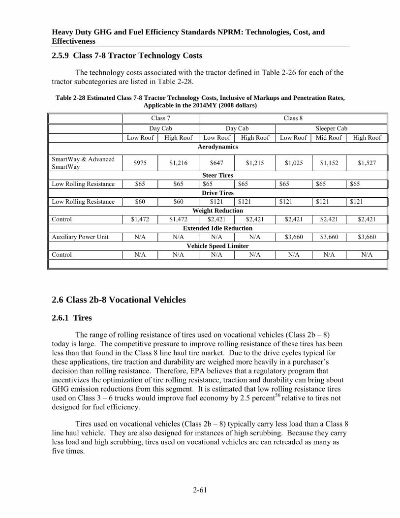
Heavy Duty GHG and Fuel Efficiency Standards NPRM: Technologies, Cost, and Effectiveness
2-61
2.5.9 Class 7-8 Tractor Technology Costs
The technology costs associated with the tractor defined in Table 2-26 for each of the tractor subcategories are listed in Table 2-28.
Table 2-28 Estimated Class 7-8 Tractor Technology Costs, Inclusive of Markups and Penetration Rates, Applicable in the 2014MY (2008 dollars)
Class 7 Class 8 Day Cab Day Cab Sleeper Cab Low Roof High Roof Low Roof High Roof Low Roof Mid Roof High Roof
Aerodynamics
SmartWay & Advanced SmartWay $975 $1,216 $647 $1,215 $1,025 $1,152 $1,527
Steer Tires Low Rolling Resistance $65 $65 $65 $65 $65 $65 $65
Drive Tires Low Rolling Resistance $60 $60 $121 $121 $121 $121 $121
Weight Reduction Control $1,472 $1,472 $2,421 $2,421 $2,421 $2,421 $2,421
Extended Idle Reduction Auxiliary Power Unit N/A N/A N/A N/A $3,660 $3,660 $3,660
Vehicle Speed Limiter Control N/A N/A N/A N/A N/A N/A N/A
2.6 Class 2b-8 Vocational Vehicles
2.6.1 Tires
The range of rolling resistance of tires used on vocational vehicles (Class 2b – 8) today is large. The competitive pressure to improve rolling resistance of these tires has been less than that found in the Class 8 line haul tire market. Due to the drive cycles typical for these applications, tire traction and durability are weighed more heavily in a purchaser’s decision than rolling resistance. Therefore, EPA believes that a regulatory program that incentivizes the optimization of tire rolling resistance, traction and durability can bring about GHG emission reductions from this segment. It is estimated that low rolling resistance tires used on Class 3 – 6 trucks would improve fuel economy by 2.5 percent56
Tires used on vocational vehicles (Class 2b – 8) typically carry less load than a Class 8 line haul vehicle. They are also designed for instances of high scrubbing. Because they carry less load and high scrubbing, tires used on vocational vehicles are can retreaded as many as five times.
relative to tires not designed for fuel efficiency.
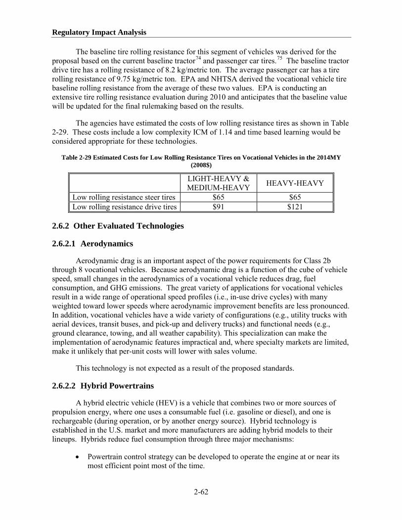
Regulatory Impact Analysis
2-62
The baseline tire rolling resistance for this segment of vehicles was derived for the proposal based on the current baseline tractor74 and passenger car tires.75
The agencies have estimated the costs of low rolling resistance tires as shown in
The baseline tractor drive tire has a rolling resistance of 8.2 kg/metric ton. The average passenger car has a tire rolling resistance of 9.75 kg/metric ton. EPA and NHTSA derived the vocational vehicle tire baseline rolling resistance from the average of these two values. EPA is conducting an extensive tire rolling resistance evaluation during 2010 and anticipates that the baseline value will be updated for the final rulemaking based on the results.
Table 2-29. These costs include a low complexity ICM of 1.14 and time based learning would be considered appropriate for these technologies.
Table 2-29 Estimated Costs for Low Rolling Resistance Tires on Vocational Vehicles in the 2014MY (2008$)
LIGHT-HEAVY & MEDIUM-HEAVY HEAVY-HEAVY
Low rolling resistance steer tires $65 $65 Low rolling resistance drive tires $91 $121
2.6.2 Other Evaluated Technologies
2.6.2.1 Aerodynamics
Aerodynamic drag is an important aspect of the power requirements for Class 2b through 8 vocational vehicles. Because aerodynamic drag is a function of the cube of vehicle speed, small changes in the aerodynamics of a vocational vehicle reduces drag, fuel consumption, and GHG emissions. The great variety of applications for vocational vehicles result in a wide range of operational speed profiles (i.e., in-use drive cycles) with many weighted toward lower speeds where aerodynamic improvement benefits are less pronounced. In addition, vocational vehicles have a wide variety of configurations (e.g., utility trucks with aerial devices, transit buses, and pick-up and delivery trucks) and functional needs (e.g., ground clearance, towing, and all weather capability). This specialization can make the implementation of aerodynamic features impractical and, where specialty markets are limited, make it unlikely that per-unit costs will lower with sales volume.
This technology is not expected as a result of the proposed standards.
2.6.2.2 Hybrid Powertrains
A hybrid electric vehicle (HEV) is a vehicle that combines two or more sources of propulsion energy, where one uses a consumable fuel (i.e. gasoline or diesel), and one is rechargeable (during operation, or by another energy source). Hybrid technology is established in the U.S. market and more manufacturers are adding hybrid models to their lineups. Hybrids reduce fuel consumption through three major mechanisms:
• Powertrain control strategy can be developed to operate the engine at or near its most efficient point most of the time.

Heavy Duty GHG and Fuel Efficiency Standards NPRM: Technologies, Cost, and Effectiveness
2-63
• The internal combustion engine can be optimized through downsizing or modifying the operating cycle. Power loss from engine downsizing can be mitigated by employing power assist from the secondary power source.
• Some of the energy normally lost as heat while braking can be captured and stored in the energy storage system for later use.
• The engine is turned off when it is not needed, such as when the vehicle is coasting or stopped, such as extending idle conditions.
Hybrid vehicles utilize some combination of the three above mechanisms to reduce fuel consumption and CO2
The effectiveness of fuel consumption and CO
emissions. A fourth mechanism to reduce fuel consumption, available only to plug-in hybrids, is by substituting the petroleum fuel energy with energy from another source, such as the electric grid. Plug-in hybrids may be suitable for some applications which travel short distances such as local pickup and delivery.
2
In addition to the purely hybrid technologies, which decreases the proportion of propulsion energy coming from the fuel by increasing the proportion of that energy coming from electricity, there are other steps that can be taken to improve the efficiency of auxiliary functions (e.g., power-assisted steering or air-conditioning) which also reduce CO
reduction depends on the utilization of the above mechanisms and how aggressively they are pursued. One area where this variation is particularly prevalent is in the choice of engine size and its effect on balancing fuel economy and performance. Some manufacturers choose not to downsize the engine when applying hybrid technologies depending on the power from the hybrid system components. In these cases, performance is improved, while fuel efficiency improves significantly less than if the engine was downsized to maintain the same performance as the conventional version. While this approach has been used in passenger cars it is more likely to be used for trucks where towing, hauling and/or cargo capacity is an integral part of their performance requirements. In these cases, if the engine is downsized, the battery can be quickly drained during a long hill climb with a heavy load, leaving only a downsized engine to carry the entire load. Because cargo capability is critical truck attribute, manufacturers are hesitant to offer a truck with downsized engine which can lead to a significantly diminished towing performance with a low battery, and therefore engines are traditionally not significantly downsized for these vehicles.
2
A hybrid drive unit is complex and consists of discrete components such as the electric traction motor, transmission, generator, inverter, controller and cooling devices. Certain types of drive units may work better than others for specific vehicle applications or performance requirements. Several types of motors and generators have been proposed for hybrid-electric drive systems, many of which merit further evaluation and development on specific
emissions and fuel consumption. Optimization of the auxiliary functions, together with the hybrid technologies, is collectively referred to as vehicle or accessory load electrification because they generally use electricity instead of engine power. Fuel efficiency gains achieved only electrification is considered in a separate section although may be combined with the hybrid system.

Regulatory Impact Analysis
2-64
applications. Series HEVs typically have larger motors with higher power ratings because the motor alone propels the vehicle, which may be applicable to Class 3-5 applications. In parallel hybrids, the power plant and the motor combine to propel the vehicle. Motor and engine torque are usually blended through couplings, planetary gear sets and clutch/brake units. The same mechanical components that make parallel heavy-duty hybrid drive units possible can be designed into series hybrid drive units to decrease the size of the electric motor(s) and power electronics.
An electrical energy storage system is needed to capture energy from the generator, to store energy captured during vehicle braking events, and to return energy when the driver demands power. This technology has seen a tremendous amount of improvement over the last decade and recent years. Advanced battery technologies and other types of energy storage are emerging to give the vehicle its needed performance and efficiency gains while still providing a product with long life. The focus on the more promising energy storage technologies such as nickel metal-hydride (NiMH) and lithium technology batteries along with ultra capacitors for the heavy-duty fleet should yield interesting results after further research and applications in the light-duty fleet.
Heavy-duty hybrid vehicles also use regenerative braking for improved fuel economy, emissions, brake heat, and wear. A conventional heavy vehicle relies on friction brakes at the wheels, sometimes combined with an optional engine retarder or driveline retarder to reduce vehicle speed. During normal braking, the vehicle’s kinetic energy is wasted when it is converted to heat by the friction brakes. The conventional brake configuration has large components, heavy brake heat sinks, and high temperatures at the wheels during braking, audible brake squeal, and consumable components requiring maintenance and replacement. Hybrid electric systems recover some of the vehicle’s kinetic energy through regenerative braking, where kinetic energy is captured and directed to the energy storage system. The remaining kinetic energy is dissipated through conventional wheel brakes or in a driveline or transmission retarder. Regenerative braking in a hybrid electric vehicle can require integration with the vehicle’s foundation (friction) braking system to maximize performance and safety. Today’s systems function by simultaneously using the regenerative features and the friction braking system, allowing only some of the kinetic energy to be saved for later use. Optimizing the integration of the regenerative braking system with the foundation brakes will increase the benefits and is a focus for continued work. This type of hybrid regenerative braking system improves fuel economy, GHG emissions, brake heat, and wear.
In addition to electric hybrid systems, EPA is experimenting with a Class 6 hydraulic hybrid that achieves a fuel economy increase superior to that of an electric hybrid.76 In this type of system, deceleration energy is taken from the drivetrain by an inline hydraulic pump/motor unit by pumping hydraulic fluid into high pressure cylinders. The fluid, while not compressible, pushes against a membrane in the cylinder that compresses an inert gas to 5,000 PSI or more when fully charged. Upon acceleration, the energy stored in the pressurized tank pushes hydraulic fluid back into the drivetrain pump/motor unit, allowing it to motor into the drivetrain and assist the vehicle’s engine with the acceleration event. This heavy-duty truck hybrid approach has been demonstrated successfully, producing good results on a number of commercial and military trucks.
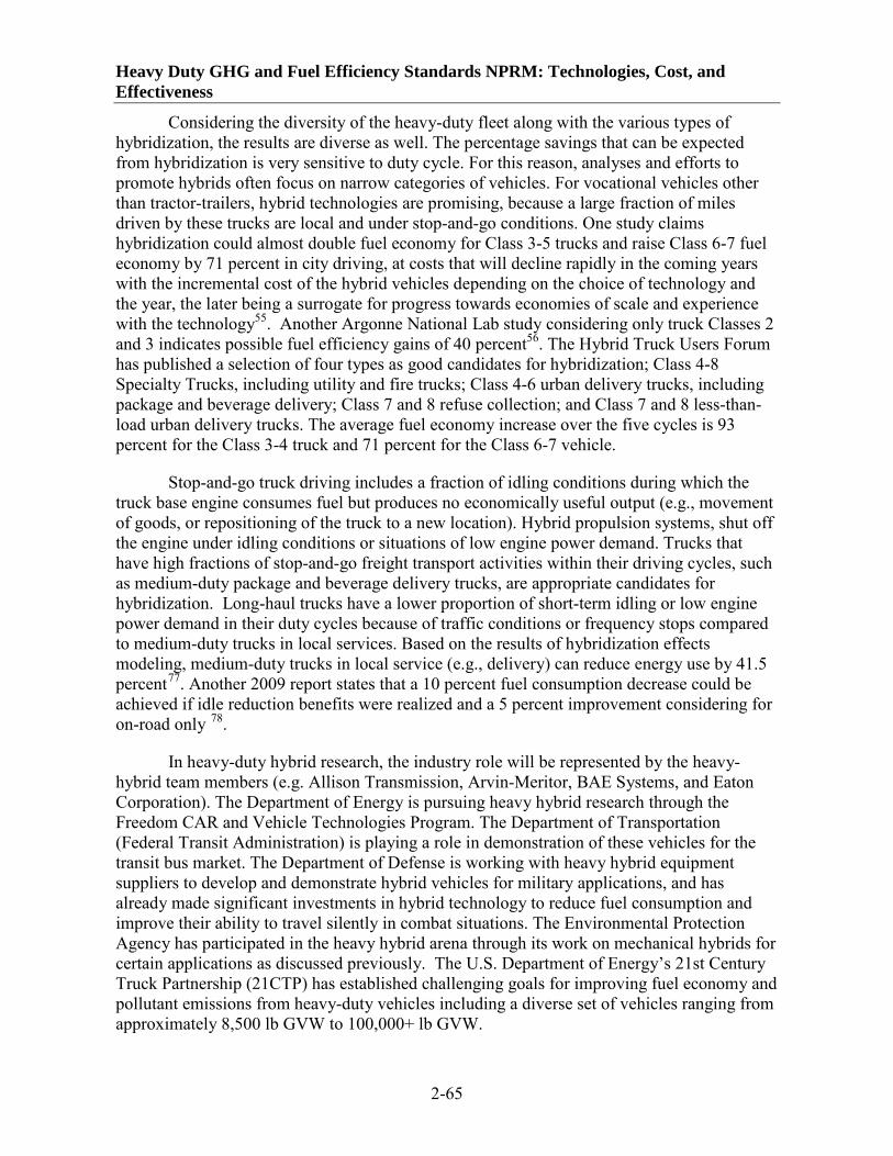
Heavy Duty GHG and Fuel Efficiency Standards NPRM: Technologies, Cost, and Effectiveness
2-65
Considering the diversity of the heavy-duty fleet along with the various types of hybridization, the results are diverse as well. The percentage savings that can be expected from hybridization is very sensitive to duty cycle. For this reason, analyses and efforts to promote hybrids often focus on narrow categories of vehicles. For vocational vehicles other than tractor-trailers, hybrid technologies are promising, because a large fraction of miles driven by these trucks are local and under stop-and-go conditions. One study claims hybridization could almost double fuel economy for Class 3-5 trucks and raise Class 6-7 fuel economy by 71 percent in city driving, at costs that will decline rapidly in the coming years with the incremental cost of the hybrid vehicles depending on the choice of technology and the year, the later being a surrogate for progress towards economies of scale and experience with the technology55. Another Argonne National Lab study considering only truck Classes 2 and 3 indicates possible fuel efficiency gains of 40 percent56. The Hybrid Truck Users Forum has published a selection of four types as good candidates for hybridization; Class 4-8 Specialty Trucks, including utility and fire trucks; Class 4-6 urban delivery trucks, including package and beverage delivery; Class 7 and 8 refuse collection; and Class 7 and 8 less-than-load urban delivery trucks. The average fuel economy increase over the five cycles is 93 percent for the Class 3-4 truck and 71 percent for the Class 6-7 vehicle.
Stop-and-go truck driving includes a fraction of idling conditions during which the truck base engine consumes fuel but produces no economically useful output (e.g., movement of goods, or repositioning of the truck to a new location). Hybrid propulsion systems, shut off the engine under idling conditions or situations of low engine power demand. Trucks that have high fractions of stop-and-go freight transport activities within their driving cycles, such as medium-duty package and beverage delivery trucks, are appropriate candidates for hybridization. Long-haul trucks have a lower proportion of short-term idling or low engine power demand in their duty cycles because of traffic conditions or frequency stops compared to medium-duty trucks in local services. Based on the results of hybridization effects modeling, medium-duty trucks in local service (e.g., delivery) can reduce energy use by 41.5 percent77. Another 2009 report states that a 10 percent fuel consumption decrease could be achieved if idle reduction benefits were realized and a 5 percent improvement considering for on-road only 78
In heavy-duty hybrid research, the industry role will be represented by the heavy-hybrid team members (e.g. Allison Transmission, Arvin-Meritor, BAE Systems, and Eaton Corporation). The Department of Energy is pursuing heavy hybrid research through the Freedom CAR and Vehicle Technologies Program. The Department of Transportation (Federal Transit Administration) is playing a role in demonstration of these vehicles for the transit bus market. The Department of Defense is working with heavy hybrid equipment suppliers to develop and demonstrate hybrid vehicles for military applications, and has already made significant investments in hybrid technology to reduce fuel consumption and improve their ability to travel silently in combat situations. The Environmental Protection Agency has participated in the heavy hybrid arena through its work on mechanical hybrids for certain applications as discussed previously. The U.S. Department of Energy’s 21st Century Truck Partnership (21CTP) has established challenging goals for improving fuel economy and pollutant emissions from heavy-duty vehicles including a diverse set of vehicles ranging from approximately 8,500 lb GVW to 100,000+ lb GVW
.
.

Regulatory Impact Analysis
2-66
In summary, many technologies that apply to cars do not apply to heavy-duty trucks and there is a common perception that investments in passenger car (light-duty vehicle) technology can easily benefit heavy-duty trucks. This group of vehicles is very diverse and includes tractor-trailers, refuse and dump trucks, package delivery vehicles and buses. The life expectancy and duty cycles for heavy-duty vehicles are about ten times more demanding than those for light-duty vehicles, technologies and solutions for the fleet must be more durable and reliable. Although a new generation of components is being developed for commercial and military HEVs, more research and testing are required.
There are no simple solutions applicable for each heavy-duty hybrid application due to the large fleet variation. A choice must be made relative to the requirements and priorities for the application. Challenges in motor subsystems such as gear reductions and cooling systems must be considered when comparing the specific power, power density, and cost of the motor assemblies. High speed motors can significantly reduce weight and size, but they require speed reduction gear sets that can offset some of the weight savings, reduce reliability and add cost and complexity. Air-cooled motors are simpler and generally less expensive than liquid-cooled motors, but they will be larger and heavier, and they require access to ambient air, which can carry dirt, water, and other contaminants. Liquid-cooled motors are generally smaller and lighter for a given power rating, but they may require more complex cooling systems that can be avoided with air-cooled versions. Various coolant options, including water, water-glycol, and oil, are available for liquid-cooled motors but must be further researched for long term durability. Electric motors, power electronics, electrical safety, regenerative braking, and power-plant control optimization have been identified as the most critical technologies requiring further research to enable the development of higher efficiency hybrid electric propulsion systems.
In addition, because manufacturers will incur expenses in bringing hybrids to market, and because buyers do not purchase vehicles on the basis of net lifetime savings, the cost-effectiveness of hybrids may not in itself translate into market success, and measures to promote hybrids are needed until costs come down. Vocational vehicles have diverse duty cycles, and they are used to a far greater extent for local trips. Some of the technologies are much less effective for trucks that generally drive at low speeds and therefore have limited applicability. Conversely, these trucks are the best candidates for hybrid technology, because local trips typically involve a large amount of stop-and-go driving, which permits extensive capture of braking and deceleration energy.
Due to the complexity of the heavy-duty fleet, the variation of hybrid system reported fuel efficiency gains and the growing research and testing – vehicle hybridization is not mandated nor included in the model for calculation of truck fuel efficiency and GHG output. Vehicle hybridization is feasible on both tractor and vocational applications but must be tested on an individual basis to an applicable baseline to realize the system benefits and net fuel usage and GHG reductions.

Heavy Duty GHG and Fuel Efficiency Standards NPRM: Technologies, Cost, and Effectiveness
2-67
2.6.2.3 EPA Testing of a Hybrid Transit Bus
EPA conducted a hybrid transit bus test to gather experience in testing hybrids and evaluate the GHG emissions and fuel consumption benefits. This section provides an overview of the study and its results.
Following coastdown testing, in-use emissions testing was conducted on each bus using portable emissions measurement systems meeting subpart J of 40 CFR 1065. Each bus was operated over two routes, which were meant to simulate normal transit bus operation. The first route was comprised entirely of typical urban stop/go driving, with a number of bus stops along the 4.75 mile route. The second route was comprised of roughly half urban driving and half highway operation, reaching a maximum speed of approximately 60 MPH. This route was approximately 5.75 miles in length.
Fuel economy could be calculated using two methods: through integration of the instantaneous fuel rate broadcast by the ECU (ECU method) or through a carbon balance of the exhaust gases (Carbon Balance Method). Both methods provided repeatable results, however the ECU method tended to consistently yield approximately 5 percent lower fuel consumption on both vehicles. This bias appears to be due to small differences in predicted fuel flow versus measured exhaust carbon, particularly during deceleration where the ECU predicts a complete fuel cut-off. Since the carbon balance method yields more conservative results, all fuel consumption data presented has been calculating using this method.
Figure 2-1 presents a comparison of the fuel economy of both buses over the two test routes. Each vehicle was tested at least 3 times over each route, and in several cases up to 10 repeats of each route were conducted. The error bars represent the standard deviation over the replicates of each route. Over both routes, the hybrid showed a significant fuel economy benefit over the conventional bus. Over route 1 (urban only), this benefit was greatest and approached 37 percent. Over route 2 (mixed urban/highway), fuel economy was still improved by over 25 percent. Much of this benefit is likely attributable to the regenerative braking and launch assist capability of the hybrid system since there is no idle shut-off of the engine. A secondary benefit to the regenerative braking system is a significant increase in brake service intervals, which was highlighted in discussions with a bus fleet operator.

Regulatory Impact Analysis
2-68
Figure 2-1 Hybrid and Conventional Bus Fuel Economy (mpg)
Fuel Economy vs Route
5.525.15
6.957.04
0.0
1.0
2.0
3.0
4.0
5.0
6.0
7.0
8.0
Route 1 Route 2
Fuel
Eco
nom
y (m
pg)
ConventionalHybrid
Figure 2-2 presents the CO2 Figure 2-3
emissions over each route on a work-specific basis. For comparison, , presents CO2 normalized by the mileage travelled. Characterizing the CO2 reduction due to the hybrid system, both methods show significant decreases in emissions. The work-specific basis may provide a more accurate comparison in this case, since environmental effects are better accounted for (i.e. driver aggressiveness, traffic, etc). This is evident when comparing the variation over the course of testing, represented by the standard deviation. The variability on a work-specific basis is nearly half that of using the distance-based metric.

Heavy Duty GHG and Fuel Efficiency Standards NPRM: Technologies, Cost, and Effectiveness
2-69
Figure 2-2 Hybrid and Conventional Bus CO2
CO2 Emissions vs Route
602624
410396
0
100
200
300
400
500
600
700
Route 1 Route 2
CO
2 (g
/bhp
-hr)
ConventionalHybrid
Emission Rates (g/bhp-hr)
Figure 2-3 Hybrid and Conventional Bus CO2
CO2 Emissions vs Route
18591995
14671442
0
500
1000
1500
2000
2500
Route 1 Route 2
CO
2 (g
/mile
)
ConventionalHybrid
Emission Rates (g/mile)
Figure 2-4 (a-d) compares the CO2 emissions rate (in g/s) during typical launch (starting from a stop) events in both buses. Both vehicles showed a spike in CO2 emissions when starting from a stop. However, this spike was much more attenuated with the hybrid bus, which demonstrates the ability of the launch assist system to reduce CO2
Figure 2-4
emissions. The magnitude of this attenuation varied depending on the exact event, however reductions of over 50 percent were not uncommon. Also worth noting is that near the 0.35 mile mark on
-d (lower-right), the CO2 emissions are near zero, suggesting that the vehicle is maintaining a speed of approximately 15 MPH solely on electric power.

Regulatory Impact Analysis
2-70
Figure 2-4 Hybrid and Conventional Bus CO2
0
5
10
15
20
25
30
35
40
45
50
0 0.1 0.2Distance (miles)
Spee
d (M
PH) o
r CO
2 (g
/s)
Conv-MPHHybrid-MPHConv - CO2Hybrid-CO2
Emission Rates (g/s)
0
5
10
15
20
25
30
35
40
45
50
0.1 0.2 0.3Distance (miles)
Spee
d (M
PH) o
r CO
2 (g
/s)
Conv-MPHHybrid-MPHConv - CO2Hybrid-CO2
a b
0
5
10
15
20
25
30
35
40
45
50
0 0.1 0.2Distance (miles)
Spee
d (M
PH) o
r CO
2 (g
/s)
Conv-MPHHybrid-MPHConv - CO2Hybrid-CO2
0
5
10
15
20
25
30
35
40
45
50
0.2 0.3 0.4Distance (miles)
Spee
d (M
PH) o
r CO
2 (g
/s)
Conv-MPHHybrid-MPHConv - CO2Hybrid-CO2
c d
Other observations through this testing suggest significant complexity in the calibration of the hybrid powertrain, presumably with the intent of reducing fuel consumption. One example is the set of engine speed-torque points over a give route (see Figure 2-5). The calibration of the hybrid powertrain (red) shows distinct patterns for where the engine operates. First, the engine is less frequently loaded at, or near idle speed. Second, the engine frequently operates at 1200 RPM, which is the lowest speed at which peak torque is available. Third, when more power is required (beyond 100 percent torque at 1200 RPM), the engine tends to operate along the maximum torque curve as RPM is increased. Keeping engine speed as low as possible reduces frictional losses, thus increasing efficiency. In contrast, the speed-torque points of the conventional bus show a much more random distribution and propensity for operating at lower engine loads.

Heavy Duty GHG and Fuel Efficiency Standards NPRM: Technologies, Cost, and Effectiveness
2-71
Figure 2-5 Hybrid and Conventional Bus Operating Map Comparison
0
20
40
60
80
100
120
500 1000 1500 2000 2500Engine Speed (RPM)
Engi
ne L
oad
(%)
ConventionalHybrid
In summary, the hybrid powertrain has demonstrated significant opportunity for reduction of fuel consumption and CO2 emissions in transit bus applications. Testing over typical bus routes showed up to a 37 percent reduction in both fuel consumption and CO2
Table 2-30
emissions. A summary of these finding is presented in . These reductions can be attributed to three features of the hybrid powertrain. First, electric launch assist facilitated through regenerative braking. Second, calibration of the engine to operate in the most efficient regions of the speed-torque map. Third, electric-only drive at lower speeds was witnessed occasionally.
Table 2-30 Hybrid Powertrain Benefit
Conventional Hybrid Benefit
Avg CoV Avg CoV mpg or g/mile
percent
Route 1 MPG 5.15 8.2% 7.04 5.5% 1.89 37%
CO2 1995 (g/mile) 8.0% 1442 5.5% 553 28%
CO2 624 (g/bhp-hr) 3.7% 396 5.3% 228 37%
Route 2 MPG 5.52 8.0% 6.95 5.3% 1.43 26%
CO2 1859 (g/mile) 7.9% 1467 5.5% 392 21%
CO2 602 (g/bhp-hr) 4.0% 410 1.7% 192 32%

Regulatory Impact Analysis
2-72
2.6.2.4 Transmission and Driveline
This technology is not expected to change as a result of the proposed standards.
2.7 Air Conditioning
Air conditioning (A/C) systems contribute to GHG emissions in two ways – direct emissions through refrigerant leakage and indirect exhaust emissions due to the extra load on the vehicle’s engine to provide power to the air conditioning system. Hydrofluorocarbon (HFC) refrigerants, which are powerful GHG pollutants, can leak from the A/C system. This includes the direct leakage of refrigerant as well as the subsequent leakage associate with maintenance and servicing, and with disposal at the end of the vehicle’s life. No other vehicle system has associated GHG leakage.79 The current refrigerant – R134a, has a high global warming potential (GWP) of 1430. 80 Due to the high GWP of this HFC, a small leakage of the refrigerant has a much greater global warming impact than a similar amount of emissions of CO2
Heavy-duty air conditioning systems today are similar to those used in light-duty applications. However, differences may exist in terms of cooling capacity (such as sleeper cabs have larger cabin volumes than day cabs), system layout (such as the number of evaporators), and the durability requirements due to longer truck life. However, the component technologies and costs to reduce direct HFC emissions are similar between the two types of vehicles.
or other mobile source GHGs.
The quantity of indirect GHG emissions from A/C use in heavy-duty trucks relative to the CO2
2.7.1 Refrigerant Leakage
emissions from driving the vehicle and moving freight is very small. Therefore, a credit approach for improved A/C system efficiency is not appropriate for this segment of vehicles because the value of the credit is too small to provide sufficient incentive to utilize feasible and cost-effective air conditioning leakage improvements. For the same reason, including air conditioning leakage improvements within the main standard would in many instances result in lost control opportunities. Therefore, EPA is proposing that truck manufacturers be required to meet a low leakage requirement for all air conditioning systems installed in 2014 model year and later trucks, with one exception. The agencies are not proposing leakage standards for Class 2b-8 Vocational Vehicles at this time due to the complexity in the build process and the potential for different entities besides the chassis manufacturer to be involved in the air conditioning system production and installation, with consequent difficulties in developing a regulatory system.
Based on measurements from 300 European light-duty vehicles (collected in 2002 and 2003), Schwarz and Harnisch estimate that the average HFC direct leakage rate from modern A/C systems was estimated to be 53 g/yr.81 This corresponds to a leakage rate of 6.9 percent per year. This was estimated by extracting the refrigerant from recruited vehicles and comparing the amount extracted to the amount originally filled (as per the vehicle specifications). The fleet and size of vehicles differs from Europe and the United States, therefore it is conceivable that vehicles in the United States could have a different leakage

Heavy Duty GHG and Fuel Efficiency Standards NPRM: Technologies, Cost, and Effectiveness
2-73
rate. The authors measured the average charge of refrigerant at initial fill to be about 747 grams (it is somewhat higher in the U.S. at 770g), and that the smaller cars (684 gram charge) emitted less than the higher charge vehicles (883 gram charge). Moreover, due to the climate differences, the A/C usage patterns also vary between the two continents, which may influence leakage rates.
Vincent et al., from the California Air Resources Board estimated the in-use refrigerant leakage rate to be 80 g/yr.82
Since the A/C systems are similar in design and operation between light- and heavy-duty vehicles, and emissions due to direct refrigerant leakage are significant in all vehicle types, EPA is proposing a leakage standard which is a “percent refrigerant leakage per year” to assure that high-quality, low-leakage components are used in each air conditioning system design. The agency believes that a single “gram of refrigerant leakage per year” would not fairly address the variety of air conditioning system designs and layouts found in the heavy-duty truck sector. EPA is proposing a standard of 1.50 percent leakage per year for Heavy-Duty Pickup Trucks and Vans and Class 7/8 Tractors. The proposed standard was derived from the vehicles with the largest system refrigerant capacity based on the Minnesota GHG Reporting database.
This is based on consumption of refrigerant in commercial fleets, surveys of vehicle owners and technicians. The study assumed an average A/C charge size of 950 grams and a recharge rate of 1 in 16 years (lifetime). The recharges occurred when the system was 52 percent empty and the fraction recovered at end-of-life was 8.5 percent.
83 Figure 2-6 As shown in , the average percent leakage per year of the 2010 model year vehicles in the upper quartile in terms of refrigerant capacity was 1.60 percent (for reference, in the 2010 Light-Duty GHG rule, the average was estimated to be 2.7 percent, based on a leakage rate of 20.7 g/yr and a system capacity of 770 g).

Regulatory Impact Analysis
2-74
0.0000
0.0200
0.0400
0.0600
0.0800
0.1000
0.1200
0.1400
0.1600
0.00 0.10 0.20 0.30 0.40 0.50 0.60 0.70 0.80 0.90 1.00 1.10 1.20 1.30 1.40 1.50 1.60 1.70 1.80 1.90 2.00 2.10 2.20 2.30 2.40 2.50 2.60 2.70 2.80 2.90 3.00
Freq
uenc
y
Annual Percentage Refrigerant Loss (%/yr)
- Annual Percentage Loss = Yearly Leak Rate / Refrigerant Capacity- 53 vehicles in data set (2010 model year only)- System refrigerant capacity ranges from 810 g (Chevrolet Express)to 1531 g (Ford E-Series w/dual evaporators)
- Yearly % leak rate ranges from 0.78%/yr (Chevrolet Express) to2.77%/yr (Toyota Land Cruiser w/dual evaporator and coolbox)
Median = 1.44 %/yrAverage = 1.60 %/yr
Figure 2-6 Distribution of Percentage Refrigerant Loss Per Year - Vehicles in Upper Quartile of A/C System Refrigerant Capacity (from 2010 Minnesota Reporting Data).
By requiring that all heavy-duty trucks achieve the proposed leakage level of 1.50 percent per year, roughly half of the vehicles in the 2010 data sample would need to reduce their leakage rates, and an emissions reduction roughly comparable to that necessary to generate direct emission credits under the light-duty vehicle program would result. See 75 FR at 25426-247. We believe that a yearly system leakage approach will assure that high-quality, low-leakage, components are used in each A/C system design, and we expect that manufacturers will reduce A/C leakage emissions by utilizing improved, leak-tight components. Some of the improved components available to manufacturers are low-permeation flexible hoses, multiple o-ring or seal washer connections, and multiple-lip compressor shaft seals. The availability of low leakage components is being driven by the air conditioning credit program in the light-duty GHG rule (which applies to 2012 model year and later vehicles). EPA believes that reducing A/C system leakage is both highly cost-effective and technologically feasible. The cooperative industry and government Improved Mobile Air Conditioning (IMAC) program has demonstrated that new-vehicle leakage emissions can be reduced by 50 percent by reducing the number and improving the quality of the components, fittings, seals, and hoses of the A/C system.84
All of these technologies are already in commercial use and exist on some of today’s systems.

Heavy Duty GHG and Fuel Efficiency Standards NPRM: Technologies, Cost, and Effectiveness
2-75
EPA proposes that manufacturers demonstrate improvements in their A/C system designs and components through a design-based method. The proposed method for calculating A/C Leakage is based closely on an industry-consensus leakage scoring method, described below. This leakage scoring method is correlated to experimentally-measured leakage rates from a number of vehicles using the different available A/C components. Under the proposed approach, manufacturers would choose from a menu of A/C equipment and components used in their vehicles in order to establish leakage scores, which would characterize their A/C system leakage performance and calculate the percent leakage per year as this score divided by the system refrigerant capacity.
Consistent with the Light-Duty Vehicle Greenhouse Gas Emissions rulemaking, EPA is proposing that a manufacturer would compare the components of its A/C system with a set of leakage-reduction technologies and actions that is based closely on that being developed through IMAC and the Society of Automotive Engineers (as SAE Surface Vehicle Standard J2727, August 2008 version).85
2.7.2 System Efficiency
See generally 75 FR at 25426. The SAE J2727 approach was developed from laboratory testing of a variety of A/C related components, and EPA believes that the J2727 leakage scoring system generally represents a reasonable correlation with average real-world leakage in new vehicles. Like the IMAC approach, our proposed approach would associate each component with a specific leakage rate in grams per year identical to the values in J2727 and then sum together the component leakage values to develop the total A/C system leakage. However, in the heavy-duty truck program, the total A/C leakage score is then divided the value by the total refrigerant system capacity to develop a percent leakage per year value.
The agencies can also develop a program that includes efficiency improvements. CO2-equivalent emissions are also associated with air conditioner efficiency, since air conditioners create load on the engine. See 74 FR at 49529. However, EPA is not proposing to set air conditioning efficiency standards for heavy-duty trucks, as the CO2 emissions due to air conditioning systems in heavy-duty trucks are minimal (compared to their overall emissions of CO2). For example, EPA conducted modeling of a Class 8 sleeper cab using GEM to evaluate the impact of air conditioning and found that it leads to approximately 1 gram of CO2/ton- mile. Therefore, a projected 24 percent improvement of the air conditioning system (the level projected in the light-duty GHG rulemaking), would only reduce CO2 emissions by less than 0.3 g CO2/ton-mile, or approximately 0.3 percent of the baseline Class 8 sleeper cab CO2
2.8 Trailers and GHG Emission Reduction Opportunities
emissions.
Trailers for use with HD tractors are an important aspect of the GHG emission performance of combination tractors and are estimated to be responsible for 11 to 12 percent of fuel consumed by Class 8 combination tractors. Optimizing the tractor and trailer as a system allows designers to take full advantage of the GHG emission reduction opportunities and, in some cases (e.g., aerodynamic drag reduction), the performance of emission reduction approach is dependent upon the tractor and trailer working in concert. For example, when

Regulatory Impact Analysis
2-76
designing a tractor’s roofline it is important to understand the type and physical characteristics of the trailer for which it is intended for use. If the roofline of the tractor and trailer are mismatched, it can result in a large, post-tractor wake (i.e., the tractors roofline is taller than that of the trailer) or present a large, drag inducing surface (i.e., the trailer front is taller than the top of the tractor). Even though trailers are an integral part of a combination tractor’s ultimate GHG emissions and fuel consumption, trailer design has remained relatively unchanged when compared to the progress made in tractors. The impacts of incorporating improved GHG emission and fuel saving performance into trailers can have long lasting impacts since trailers are often kept in service for longer periods than tractors.
2.8.1 Current Trailer Fleet
There are approximately 5.6 million HD trailers on the roads today86
Table 2-31
. In general, it is common to have roughly 3 trailers for every tractor to facilitate efficiency in loading and
unloading operations. Serving a wide range of needs, this trailer fleet is necessarily comprised of a wide range of trailer types including box van (including refrigerated units), shipping container (e.g., 20 and 40 foot ocean-going container) chassis, flat bed (including
drop deck units), dump, tanker, and specialty (e.g., grain, livestock, auto-carriers). Types of trailers can be further subdivided by their length and height. The vast majority of HD trailers on the road are box van trailers that are 53 feet long. presents the current market
share of major types of trailers.87

Heavy Duty GHG and Fuel Efficiency Standards NPRM: Technologies, Cost, and Effectiveness
2-77
Table 2-31: Composition of Current Heavy-Duty Trailer Fleet
TRAILER TYPE MARKET SHARE1
Box, van (53’)
(PERCENT) 45
Box, van (40 – 52’) 6 Box, van (24 – 39’) 9 Box, van (refrigerated) 5 Container chassis 7 Dump 3 Flatbed 8 Flatbed (drop deck) 2 Grain 2 Tagalong 4 Tagalong (enclosed) 2 Other 9
Diversity in the trailer fleet is not limited to the types of trailers on the road but also extends to the owners and operators of trailers. Trailers are owned and operated by individual fleets, logistics companies that move goods for others, and government entities.
While approximately 10 companies manufacture approximately 80 percent of the trailers sold, the entire trailer market includes a large number of trailer producers. 88
2.8.2 Trailer Technologies to Reduce GHG Emissions
Only 14 manufacturers have an annual sales volume of greater than 3,000 trailers with many specializing in a type of trailer (e.g., grain, dump, tanker).
Technologies for use on trailers that reduce GHG emissions and fuel consumption are commercially available. These include aerodynamic devices, low rolling resistance tires, and weight reduction. Trailer systems that allow a tractor to move more goods such as double trailer configurations (e.g., Rocky Mountain Doubles with 28 or 48 foot trailers) can also be considered as trailer strategies to reduce GHG emissions. Of these technologies, trailer aerodynamics and low rolling resistance tires have gained wide acceptance and are discussed in detail below.
2.8.2.1 Trailer Aerodynamics
Trailer aerodynamic technologies have focused on the box, van trailers – the largest segment of the trailer fleet. This focus on box, van trailers may also be partially attributed to the complexity of the shape of the non-box, van trailers which, in many cases, transport cargo that is in the windstream (e.g., flatbeds that carry heavy equipment, car carriers, and loggers). For non-box, van trailers you could have a different aerodynamic shape with every load.

Regulatory Impact Analysis
2-78
While some technologies exist to address aerodynamic drag for non-box, van trailers, it has been either experimental or not widely commercially available.
Current trailer aerodynamic technologies for box, van trailers are estimated to provide approximately 7 percent GHG emission reductions when used as a package. For box, van trailers, trailer aerodynamic technologies have addressed drag at the front of the trailer (i.e., vortex traps, leading edge fairings), underneath the trailer (i.e., side skirts, wheel fairings) and the trailer rear (i.e., afterbodies). These technologies are commercially available and have seen moderate adoption rates. Table 2-32 shows technologies that have generally been accepted for use on box, van trailers. In general, the performance of these technologies is dependent upon the smooth transition of airflow from the tractor to the trailer. True for both tractor and trailer aerodynamic drag reduction, the overall shape can be optimized to minimize aerodynamic drag and, in fact, the trailer body must have at least a moderately aerodynamic shape (and its relatively smooth flow) to benefit from add-on aerodynamic components.
Table 2-32: Trailer Technologies to Address Aerodynamic Drag
LOCATION ON TRAILER
TECHNOLOGY TYPE DESIGNED EFFECT
Front Vortex trap Reduce drag induced by cross-flow through gap between tractor and trailer
Front Front fairings Smoothly transition air to flow from tractor to the trailer
Rear Afterbody (boat tail and rear fairings)
Reduce pressure drag induced by the trailer wake
Undercarriage Side skirts Manage flow of air underneath tractor to reduce eddies and wake
Undercarriage Underbelly treatment Manage flow of air underneath tractor to reduce eddies and wake
Accessories General Reducing surface area perpendicular to travel and minimizing complex shapes that may induce drag
General Advanced, passive air management
Manage airflow through passive aerodynamic shapes or devices that keep flow attached to the vehicle (tractor and trailer)
Table 2-33 Trailer Technologies Incremental Costs
TECHNOLOGY COST ESTIMATE Trailer Side Skirts $1300 – 1600 Gap Fairing $850 Trailer Aerocone $1000 Boat Tails $1960 Air Tabs $180

Heavy Duty GHG and Fuel Efficiency Standards NPRM: Technologies, Cost, and Effectiveness
2-79
2.8.2.2 Tires – Single Wide and Low Rolling Resistance
Beginning in 2007, EPA began designating certain new dry freight box van trailers for on the road use of 53 feet or greater length Certified SmartWay Trailers. Older or pre-owned trailers could also be certified if properly retrofitted. In order for a trailer to be designated as Certified SmartWay, the trailer must be equipped with verified low rolling resistance trailer tires (either dual or single-wide), among other things.
The RRc baseline for today’s fleet is 6.5 kg/metric ton for the trailer tire, based on sales weighting of the top three manufacturers based on market share. This value is based on new trailer tires, since rolling resistance decreases as the tread wears. To achieve the intended emissions benefit, SmartWay established the maximum allowable RRc
Research indicates the contribution to overall vehicle fuel efficiency by tires is approximately equal to the proportion of the vehicle weight on them
for the trailer tire 15 percent below the baseline or 5.5 kg/metric ton.
. On a fully loaded typical Class 8 long-haul tractor and trailer, 42.5 percent of the total tire energy loss attributed to rolling resistance is from the trailer tires.
The Center for Transportation Research at Argonne National Laboratory analyzed technology options to support energy use projections. EPA agrees with their assumed incremental cost of low rolling resistance tires of $15 - $20 per tire. With 8 tires replaced on a trailer, the incremental cost would be between $120 and $160. Often the steer tire is retreaded and placed on the trailer axle. There is a cost savings associated with retread tires. A new retread costs between $150 and $200, compared to a new tire which costs typically around $400. This represents a savings of $1,200 to $1,600 per trailer.
Single wide tires are also used on trailers. The Center for Transportation Research estimated incremental capital cost of single wide tires is $30 - $40 per tire. With 4 single wide tires replacing 8 dual tires on the trailer, the incremental cost would be between $120 and $160.
Based on the ICF report,89
2.8.2.3 Trailer Weight Reduction
EPA and NHTSA estimate the incremental retail cost for low rolling resistance tires as $78 per tire. The agencies also estimate that the incremental cost to replace a pair of dual tires with a single wide based tire is $216, however, the cost can be reduced when the wheel replacement cost is considered.
Weight reduction opportunities in trailers exist in both the structural components and in the wheels and tires. Material substitution (replacing steel with aluminum) is feasible for components such as roof posts, bows, side posts, cross members, floor joists, and floors. Similar material substitution is feasible for wheels. Weight reduction opportunities also exist through the use of single wide based tires replacing two dual tires.

Regulatory Impact Analysis
2-80
The agencies’ assessment of the ICF report indicates that the expected incremental retail prices of the lightweighted components are as included in Table 2-34 Trailer Lightweighting Incremental Costs.
Table 2-34 Trailer Lightweighting Incremental Costs
COMPONENT COST Roof Posts/Bows $120 Side Posts $525 Cross Members/Floor Joists $400 Floor $1,500 Wheels $1,500
2.8.2.4 Opportunities in Refrigerated Trailers
Refrigeration units are used in van trailers to transport temperature sensitive products. A traditional trailer refrigeration unit (TRU) is powered by a nonroad diesel engine. There are GHG reduction opportunities in refrigerated trailers through the use of electrical trailer refrigeration units and highly reflective trailer coatings.
Highly reflective materials, such as reflective paints or translucent white fiberglass roofs, can reflect the solar radiation and decrease the cooling demands on the trailer’s refrigeration unit. A reflective composite roof can cost approximately $800, the addition of reflective tape to a trailer roof would cost approximately $450.
Hybrid TRUs utilize a diesel engine which drives a generator which in turn powers the compressor and fans. The cost of this unit is approximately $4,000.
All-electric TRUs, needing no diesel engine to power the unit, are being tested in U.S. refrigerated fleets. There is no market price for these units at this time.
2.9 Other Fuel Consumption and GHG Reducing Strategies
There are several other types of strategies available to reduce fuel consumption and GHG emissions from trucks. EPA and NHTSA identify several of these technologies and strategies below, but acknowledge that they are outside the proposed regulatory framework currently identified.
2.9.1 Auxiliaries
The accessories on a truck engine, including the alternator, coolant and oil pumps are traditionally mechanically gear or belt driven by the base engine. In general, the effect of accessory power consumption in trucks is much less than in cars but the mechanical auxiliaries operate whenever base engines are running, which can waste energy when the auxiliaries are not needed. The replacement of mechanical auxiliaries by electrically driven systems can decouple mechanical loads from the base engine and reduce energy use. Since the average engine loads from mechanical auxiliaries are higher than those from a small generator that supplies electricity to electric auxiliaries, base engine fuel can be reduced. A

Heavy Duty GHG and Fuel Efficiency Standards NPRM: Technologies, Cost, and Effectiveness
2-81
reduction in CO2
• Air compressor,
emissions and fuel consumption can be realized by driving them electrically and only when needed (“on-demand”). The heavy and medium trucks have several auxiliary systems:
• Hydraulic pumps, • Coolant pump, • Engine oil and fuel pumps, • Fans, and • Air conditioning compressor.
The systems listed above, although not inclusive, can be optimized by various methods reducing fuel consumption and GHG emissions;
• Electric power steering (EPS) – is an electrically-assisted steering system that has advantages over traditional hydraulic power steering because it replaces a continuously operated hydraulic pump, thereby reducing parasitic losses from the accessory drive.
• Electric water pumps and electric fans - can provide better control of engine cooling.
For example, coolant flow from an electric water pump can be reduced and the radiator fan can be shut off during engine warm-up or cold ambient temperature conditions which will reduce warm-up time, reduce warm-up fuel enrichment, and reduce parasitic losses. Indirect benefit may be obtained by reducing the flow from the water pump electrically during the engine warm-up period, allowing the engine to heat more rapidly and thereby reducing the fuel enrichment needed during cold starting of the engine.
• High efficiency alternators - provide greater electrical power and efficiency at road
speed or at idle than conventional original equipment replacement alternators that typically operate at 55 percent efficiency.
• If electric power is not available - there are still some technologies that can be applied
to reduce the parasitic power consumption of accessories. Increased component efficiency is one approach, and clutches can be used to disengage the alternator and air compressor when they are not required. Many MD/HD engines incorporate clutched cooling fans which can be shut off during engine warm-up thereby not requiring electric cooling fans. Air compressors that are rotating but not creating pressure absorb about half the power of a pumping compressor, and compressors normally only pump a small percentage of the time in long-haul trucks.
Several studies have documented the GHG reductions from electrification and/or optimization of truck auxiliaries. One study, based on a full-scaled test of a prototype truck that used a small generator to produce electricity, full electrification of auxiliaries reduces fuel use by 2 percent including extended idle and estimated potential reductions in modal GHG emissions are 1.4 percent. Another study recently completed by Ricardo discussed the advantages of electrification of engine accessories along with the potential to increase fuel

Regulatory Impact Analysis
2-82
economy citing examples such as variable flow water pumps and oil pumps90
Accurate data providing power consumption values for each discrete accessory over a range of operating conditions was not available due to the variation of the truck fleet. Based on research and industry feedback, a simplified assumption for modeling was made that the average power demand for mechanically driven accessories is 5 kW, and the average power demand for electrically driven accessories is 3 kW. This provides a 2 kW advantage for the electrically driven accessories over the entire drive cycle represent and is estimated to provide a 1.5 percent improvement in efficiency and reduction in CO
. Potential gains may be realized in the range of 1 to 3 percent but are highly dependent on truck type, size and duty cycle. In a NESCAFF study, the accessory power demand of a baseline truck was modeled as a steady state power draw of 5 kW, and 3 kW for more electrical accessories in individual vehicle configurations that included electric turbo compounding. The 2 kW savings versus average engine power of 100 to 200kW over a drive cycle nets roughly 1 to 2 percent savings compared to a baseline vehicle.
2
2.9.2 Driver training
emissions. As a comparison, the average load on a car engine over a drive cycle may be in the 10 to 20 kW range. At this level, a 2 kW reduction in accessory loads of a passenger vehicle makes a significant difference (approximately 10 percent). Given the higher loads experienced by truck engines, accessory demand is a much smaller share of overall fuel consumption. Accessory power demand determined by discrete components will be not be included in the model at this time and a power draw of 5 kW for standard accessories and 3 kW for electrical accessories will be used. There is opportunity for additional research to improve upon this simple modeling approach by using actual measured data to improve the modeling assumptions.
Driver training that targets fuel efficiency can help drivers recognize and change driving habits that waste fuel and increase harmful emissions. Even highly experienced truck drivers can boost their skills and enhance driving performance through driver training programs.91
Driving habits that commonly waste fuel are high speed driving, driving at unnecessarily high rpm, excessive idling, improper shifting, too-rapid acceleration, unnecessarily frequent stops and starts, and poor route planning. Well-trained drivers can reduce fuel consumption by applying simple techniques to address vehicle and engine speed, shifting patterns, acceleration and braking habits, idling, and use of accessories.
92 Some techniques include starting out in a gear that does not require using the throttle when releasing the clutch, progressive shifting (upshifting at the lowest possible rpm), anticipating traffic flow to reduce starts and stops, use of block shifting where possible (e.g., shifting from 2nd to 5th
As discussed elsewhere in this chapter, idling can be eliminated by the use of auxiliary power units or other idle reduction solutions that provide power or heating and cooling to the cab at a much lower rate of energy consumption.
gear), using cruise control as appropriate, and coasting down or using the engine brake to slow the vehicle, instead of gearing down or using the brake pedal.

Heavy Duty GHG and Fuel Efficiency Standards NPRM: Technologies, Cost, and Effectiveness
2-83
Better route planning that reduces unnecessary mileage and the frequency of empty backhauls, and takes into account factors like daily congestion patterns is another facet of a comprehensive driver training program. Such planning can be assisted through the use of logistics companies, which specialize in such efficiencies.
In its report, Technologies and Approaches to Reducing the Fuel Consumption of Medium and Heavy-Duty Vehicles, the National Research Council cited studies that found, on average, a five percent improvement in vehicle fuel efficiency due to driver training.93 EPA’s SmartWay Transport Partnership has documented the success of dozens of trucking companies’ use of driver training programs. One company reported saving an average of 42 gallons per student, or 335,000 gallons of fuel per year; and, saving 837,000 gallons of fuel in the four years it has had its training program in place.94
While EPA and NHTSA recognize the potential opportunity to reduce fuel consumption and greenhouse gas emissions by encouraging fuel-efficient driver habits, mandating driver training for all of the nation’s truck drivers is beyond the scope of this proposed regulation. However, in developing this proposal, the agencies did consider technologies that can provide some of the benefits typically addressed through driver training. Examples include automatic engine shutdown to reduce idling, automated or automated manual transmissions to optimize shifting, and speed limiters to reduce high speed operation. EPA will continue to promote fuel-efficient driving through its SmartWay program. In addition to providing fact sheets on fuel efficient driving,
Trucking fleets can provide additional motivation to reward drivers for improved performance with incentive programs, which may be monetary or provide other forms of benefits and recognition. Sometimes negative measures are employed to urge compliance with company expectations, up to and including termination of employment. Successful programs are those that perform ongoing reviews of driver techniques, and provide assistance to improve and/or retrain drivers.
95
2.9.3 Automatic Tire inflation and Tire Pressure Monitoring System
SmartWay is collaborating with Natural Resources Canada’s FleetSmart program to develop a web-enabled “fuel efficient driver” training course for commercial truck drivers. Once the course is developed, it will complement the agencies regulatory program by making fuel efficient driver training strategies available to any commercial truck driver.
Underinflation of tires has the potential to reduce fuel economy by as much as two to three percent96. Although most truck fleets understand the importance of keeping tires properly inflated, it is likely that a substantial proportion of trucks on the road have one or more underinflated tires. An industry survey conducted in 2002 at two truck stops found that fewer than half of the tires checked were within five pounds of their recommended inflation pressure. Twenty-two percent of the vehicles checked had at least one tire underinflated by at least twenty pounds per square inch (psi), and four percent of the vehicles were running with at least one flat tire, defined as a tire underinflated by fifty psi or more. The survey also found mismatches in tire pressure exceeding five percent for dual tires on axle ends.97
Proper tire inflation pressure can be maintained with a rigorous tire inspection and maintenance program or with the use of tire pressure and inflation systems. These systems

Regulatory Impact Analysis
2-84
monitor tire pressure; some also automatically keep tires inflated to a specific level. However, while the agencies recognize that such devices could have a beneficial effect on fuel economy, their use is not included in the regulatory framework. Notwithstanding the cited survey, the level of underinflation of tires in the American truck fleet is not known,98 which means that neither a baseline value nor an estimate of the fuel savings from the use of automatic tire inflation systems can be quantified with certainty. Through its SmartWay program, however, EPA does provide information on proper tire inflation pressure and on tire inflation and tire inflation pressure monitoring systems.99
2.9.4 Engine Features
Previous sections 2.3.2.2 through 2.3.2.8 describe the technologies that can be tested in an engine test cell for certification purpose and could be potentially implemented in production before the time frame of 2017. Some other technologies that cannot be easily tested in an engine test cell, but can improve engine fuel economy, should be worthwhile mentioning. Examples include these technologies, such as driver rewards, load based speed control, gear down protection, and fan control offered by Cummins’s PowerSpec.
The driver reward developed by Cummins monitors and averages the driver trip fuel economy and trip idle percent time at regular intervals, seeking to modify driver behavior by offering incentives to use less fuel. Desirable driving habits, such as low percentage of idle time, and high MPG, are rewarded with higher limits on the road speed governor, cruise control or both. The load based speed control or other similar programs are designed to improve fuel economy, lower vehicle noise, and improve driver satisfaction by managing engine speed (rpm) based on real time operating conditions. During high power requirements, this type of technology enhances engine performance by providing the driver with an extended operating range. In addition to the fuel economy benefits from operating the engine at lower speeds, vehicle noise is lowered.
Gear down protection offered by Cummins is to promote increased fuel economy by encouraging the vehicle driver to operate as much as effectively possible in top gear where fuel consumption is lower. This can be done by limiting vehicle speed in lower gears. Maximizing time in top gear means the engine runs in a lower rpm range, where fuel economy is best with improved durability and without compromising performance. Difference between top gear and one gear down can be as much as 16 percent in fuel economy. More detailed descriptions of many technologies including those mentioned here can be viewed at Cummins’s website of http://www.powerspec.cummins.com/site/home/index.html.
Although these technologies mentioned in this section are not able to be tested in an engine test cell environment, thus being unable to be directly used for benefits of certification purpose, the agency encourages manufacturers to continue improving the current and developing new technologies, thereby reducing green house gases in a broader way.
2.9.5 Logistics
Logistics encompasses a number of interrelated, mostly operational factors that affect how efficiently the overall freight transport system works. These factors include choice of

Heavy Duty GHG and Fuel Efficiency Standards NPRM: Technologies, Cost, and Effectiveness
2-85
mode, carrier and equipment; packaging type and amount; delivery time; points of origin and destination; route choice, including locations of ports and distribution hubs; and transportation tracking systems. These factors are controlled by the organizations that ship and receive goods. Due to the specialized nature of logistics management, organizations increasingly rely upon internal or outsourced business units to handle this function; many transportation providers offer logistics management services to their freight customers.
Because optimizing logistics is specific to each individual freight move, neither EPA nor NHTSA believed it is feasible to manage logistics through this proposed regulation. However, implementing certain system-wide logistics enhancements on a national level could provide benefits. As described in the National Research Council’s recent report,100 a broader national approach could include enhanced telematics and intelligent transportation systems; changes to existing infrastructure to optimize modal choice; and increased truck capacity through changes to current truck weight and size limits. While such a broad transformation of our freight system is worthwhile to consider, implementing such system-wide changes falls outside the scope of this proposed regulation. As the National Research Council noted,101
2.9.6 Longer Combination Vehicles, Weight Increase
due to its complex nature, logistics management is not readily or effectively addressed through any single approach or regulation; a number of complementary measures and alternatives are needed. Such measures can include initiatives that enable companies to better understand, measure and track the benefits of logistics optimization from an environmental and economic standpoint. The SmartWay program provides uniform tools and methodologies that companies can use to assess and optimize transportation supply chains, and can complement any future regulatory and nonregulatory approaches.
Longer combination vehicles (LCVs) are tractor-trailer combinations that tow more than one trailer, where at least one of the trailers exceeds the “pup” size (typically 24-28 feet). Because LCVs are capable of hauling more freight than a typical tractor-trailer combination, using LCVs reduces the number of truck trips needed to carry the same amount of freight. On a fleetwide basis, this saves fuel, reduces greenhouse gas emissions, and reduces per-fleet shipping costs. A typical non-LCV may tow a single trailer up to 53 feet in length, or tow two pup trailers, or even be a straight truck with a pup trailer connected via a draw bar. In contrast, the typical LCV may consist of a tractor towing two trailers of 45-48 feet, and occasionally 53 feet in length (a “turnpike double”), or one of that size and one pup (a “Rocky Mountain double”), or may tow three pups (a “triple”).
Trucks consisting of a two-axle tractor combined with two one-axle trailers up to 28.5 feet are permitted on all highways in the U.S. National Network, which consists of the interstate highway system and certain other roads. Individual states may permit longer LCVs to operate on roads that are not part of the National Network. They are allowed in 16 western states, but only on turnpikes in the five states east of the Mississippi that allow them; no new states were granted permitting authority for LCVs after 1991.102 Regulations vary among states; some allow LCVs with more than three trailers, but only by permit. Longer length turnpike doubles are typically restricted to tolled turnpikes. Such restrictions are based on considerations of the difficulty of operation and on expected weather conditions. Other

Regulatory Impact Analysis
2-86
regulations on the types of LCVs allowed are seen in other countries; in Australia, “road trains” of up to four trailers, usually with three axles per trailer, are permitted.
Some proponents of liberalized size and weight regulations project substantial benefits, estimating that highway freight productivity could be doubled and costs reduced. Despite the potential benefits of LCVs, as the National Research Council noted in its recent report, there are considerations that may make LCVs less cost effective and less safe. For example, if infrastructure (e.g., bridges with sufficient capacity; roadways with adequate lane width and curb radii for turning to accommodate an LCV safely) are not available without traveling far from a more efficient route, or if there is insufficient opportunity for the LCV to make the most of the available volume in multiple trailers, then LCVs would not be cost effective.
The increased vehicular weight of LCVs is both a safety issue and a road maintenance issue (see discussion below on increasing vehicle weight and legal load limits). The additional weight of extra trailers increases braking and stopping distance, and adds difficulty in maintaining speed in grade situations.
With additional regard to safety, LCVs might have trouble with offtracking (when the truck’s front and rear wheels do not follow the same path, which can result in departing the lane boundaries—a particular problem with longer LCVs), and could increase the challenge of merging with and maneuvering in traffic. Lateral stability is a greater problem in LCVs, and leads to a greater chance of rollover, particularly when the individual trailers are shorter. Also, when a vehicle is passing a LCV on a two-lane road, the period of time spent in the opposing lane (up to 2-3 seconds) poses another safety problem.103
Moves to increase commercial vehicle weight limits concern not only relaxing limitations on the use of LCVs, but also increasing gross vehicle weight limits for single unit trucks and conventional tractor-trailer combinations, as well as increasing axle load limits and trailer lengths. Some analysts cite scenarios in which such relaxations result in increased highway freight productivity, while yielding significant reductions in shipping costs, congestion, and total vehicle miles traveled. Increasing the weight limits allows commercial freight vehicles to carry heavier loads, reducing the number of trucks required to transport freight, potentially resulting in overall emissions reductions.
Such safety considerations impact decisions regarding restrictions on the use of LCVs, even when they may otherwise be a cost effective freight choice.
Federal law limits gross vehicle weight for commercial vehicles operating in the Interstate Highway System to a maximum of 80,000 lbs. (maximum 20,000 lbs. per single axle, 34,000 lbs. per tandem axle), with permits available for certain oversize or overweight loads and exceptions allowing 400 lbs. more for tractors with idle reduction devices. Additional vehicle weight limitations have been set by state and local regulations. These limitations arise from considerations of infrastructure characteristics, traffic densities, economic activities, freight movement, mode options, and approach to transportation design. In some cases, state limits are higher than federal limits.104 While these parameters are changeable, federal weight limits on vehicles have not changed since 1982, and limits set by states have been frozen since 1991.

Heavy Duty GHG and Fuel Efficiency Standards NPRM: Technologies, Cost, and Effectiveness
2-87
In response to input from the freight transportation sector and other interested parties, the Department of Transportation, the Transportation Research Board, the General Accounting Office, and others have conducted studies examining the impacts of proposals related to liberalized weight limits. However, regardless of the potential benefits of such action, the analyses predict premature degradation of infrastructure (e.g., bridges, pavement, grades) as a consequence. Increased costs required to maintain and upgrade the highway system would impose high burdens on already-strained public resources, raising serious questions on the desirability of relaxing weight limits, and on whether such expenditures provide adequate public good to justify them. Safety issues similar to those cited for LCVs enter into this debate, as do concerns with the effect on the efficiency of automotive travel, impacts on and net productivity of other shipping modes (particularly rail), and potential environmental and social costs. The National Research Council in its recent report105
2.9.7 Traffic Congestion Mitigation
recognized the complexities and potential trade-offs involved in increasing vehicle size and weight limits. While is worthy to discuss the potential emission and energy benefits of heavier and longer trucks, the far-reaching policy ramifications extend far beyond the scope of this proposal.
There are a wide range of strategies to reduce traffic congestion. Many of them are aimed at eliminating light-duty vehicle trips such as mass transit improvements, commute trip reduction programs, ridesharing programs, implementation of high occupancy vehicle lanes, parking pricing, and parking management programs. While focused on reducing light-duty vehicle trips, these types of strategies would allow heavy- and medium-duty vehicles to travel on less congested roads and thereby use less fuel and emit less CO2
A second group of strategies would directly impact CO
.
2
Some strategies would be designed to effect trips made by heavy- and medium-duty trucks. These would include programs to shift deliveries in congested areas to off-peak hours. Another example is to modify land use so that common destinations are closer together, which reduces the amount of travel required for goods distribution.
emissions and fuel consumption from all types of vehicles. One example of these strategies is road pricing including increasing the price of driving on certain roads or in certain areas during the most congested periods of the day. A second example is reducing the speed limits on roads and implementing measures to ensure that drivers obey the lower speed limits such as increased enforcement or adding design features that discourage excessive speeds.
These types of congestion relief strategies have been implemented in a number of areas around the country. They are typically implemented either by state or local governments or in some cases strategies to reduce commuting trips and scheduling off-peak deliveries have been implemented by private companies or groups of companies.

Regulatory Impact Analysis
2-88
2.10 Summary of Technology Costs Used in this Analysis
Table 2-35 shows the technology costs used throughout this analysis for heavy-duty engines, vocational vehicles and combination tractors for the years 2014-2020. Table 2-36 shows the technology costs used throughout this analysis for Class 2b and 3 diesel and gasoline trucks for the years 2014-2020. These tables reflect the impact of learning effects on estimated technology costs. Refer to Table 2-1 for details on the ICMs applied to each technology and Table 2-2 for the type of learning applied to each technology. The costs shown in the tables do not include the penetration rates so do not always reflect the technology’s contribution to the resultant package costs. One final note of clarification is that the terms “MHDDcomb” and “HHDDcomb” in the “Class” column refer specifically to engines placed in combination tractors (Class 7 and 8 day cabs and sleeper cabs).

Heavy Duty GHG and Fuel Efficiency Standards NPRM: Technologies, Cost, and Effectiveness
2-89
Table 2-35 Technology Effectiveness and Costs, Inclusive of Markups, by Year for Heavy-duty DieselA
Technology
and Gasoline Engines, Vocational Vehicles, and Combination Tractors (2008$)
Applied to Truck type Class CO2 2014 eq
Effectiveness 2015 2016 2017 2018 2019 2020
Aftertreatment improvements Engine LHDD 1-4% $111 $108 $104 $101 $98 $96 $94
Turbo efficiency improvements Engine LHDD 1-2% $17 $17 $16 $16 $17 $17 $16
Piston improvements Engine
LHDD
0.5-2%
$3 $3 $2 $2 $2 $2 $2
Optimized water pump Engine
LHDD $87 $84 $82 $79 $77 $75 $74
Optimized oil pump Engine
LHDD $4 $4 $4 $4 $4 $4 $4
Optimized fuel pump Engine
LHDD $4 $4 $4 $4 $4 $4 $4
Valve train friction reductions Engine
LHDD $104 $101 $98 $95 $92 $90 $88
Optimized fuel rail Engine
LHDD
2-7%
$11 $11 $11 $10 $10 $10 $10
Optimized fuel injector Engine
LHDD $14 $13 $13 $13 $12 $12 $12
EGR cooler improvements Engine
LHDD $3 $3 $3 $3 $3 $3 $3
Cylinder head improvements Engine LHDD $10 $10 $10 $9 $9 $9 $9
2014 MY LHDD Engine Package Engine LHDD 5% $369 $358 $348
A The costs included in the table represent technology costs. The engineering costs of $6,750,000 per diesel engine manufacturer per year for a five year period are not included in the table.

Regulatory Impact Analysis
2-90
Technology Applied to Truck type Class CO2 2014 eq
Effectiveness 2015 2016 2017 2018 2019 2020
2017 MY LHDD Engine Package Engine LHDD 9% $337 $327 $321 $314
Aftertreatment Improvements Engine MHDD 1-4% In R&D In R&D In R&D In R&D In R&D In R&D In R&D
Turbo efficiency improvements Engine MHDD 1-2% $17 $17 $16 $16 $15 $15 $15
Piston improvements Engine MHDD
0.5-2%
$3 $3 $2 $2 $2 $2 $2 Optimized water pump Engine MHDD $87 $84 $82 $79 $77 $75 $74 Optimized oil pump Engine MHDD $4 $4 $4 $4 $4 $4 $4 Optimized fuel pump Engine MHDD $4 $4 $4 $4 $4 $4 $4 Valve train friction reductions Engine MHDD $78 $76 $73 $71 $69 $68 $66
Optimized fuel rail Engine MHDD
2-7%
$10 $9 $9 $9 $8 $8 $8 Optimized fuel injector Engine MHDD $10 $10 $10 $9 $9 $9 $9 EGR cooler improvements Engine MHDD $3 $3 $3 $3 $3 $3 $3 Cylinder head improvements Engine MHDD $6 $6 $6 $6 $5 $5 $5
2014 MY MHDD Engine Package Engine MHDD 5% $223 $216 $210
2017 MY MHDD Engine Package Engine MHDD 9% $203 $197 $193 $189
Aftertreatment Improvements Engine MHDDcomb 1-4% In R&D In R&D In R&D In R&D In R&D In R&D In R&D
Turbo efficiency improvements Engine MHDDcomb 1-2% $17 $17 $16 $16 $15 $15 $15
Piston improvements Engine MHDDcomb
0.5-2%
$3 $3 $2 $2 $2 $2 $2 Optimized water pump Engine MHDDcomb $87 $84 $82 $79 $77 $75 $74 Optimized oil pump Engine MHDDcomb $4 $4 $4 $4 $4 $4 $4 Optimized fuel pump Engine MHDDcomb $4 $4 $4 $4 $4 $4 $4 Valve train friction reductions Engine MHDDcomb $78 $76 $73 $71 $69 $68 $66
Optimized fuel rail Engine MHDDcomb
2-7%
$10 $9 $9 $9 $8 $8 $8 Optimized fuel injector Engine MHDDcomb $10 $10 $10 $9 $9 $9 $9 EGR cooler improvements Engine MHDDcomb $3 $3 $3 $3 $3 $3 $3 Cylinder head improvements Engine MHDDcomb $6 $6 $6 $6 $5 $5 $5
Turbo mechanical- Engine MHDDcomb 2.5-5% -- -- -- $823 $798 $782 $767

Heavy Duty GHG and Fuel Efficiency Standards NPRM: Technologies, Cost, and Effectiveness
2-91
Technology Applied to Truck type Class CO2 2014 eq
Effectiveness 2015 2016 2017 2018 2019 2020
compounding 2014 MY MHDD Engine Package Engine MHDDcomb 3% $223 $216 $210
2017 MY MHDD Engine Package Engine MHDDcomb 5% $1,027 $996 $976 $956
Aftertreatment Improvements Engine HHDD 1-4% In R&D In R&D In R&D In R&D In R&D In R&D In R&D
Turbo efficiency improvements Engine HHDD 1-2% $17 $17 $16 $16 $15 $15 $15
Piston improvements Engine HHDD
0.5-2%
$3 $3 $2 $2 $2 $2 $2 Optimized water pump Engine HHDD $87 $84 $82 $79 $77 $75 $74 Optimized oil pump Engine HHDD $4 $4 $4 $4 $4 $4 $4 Optimized fuel pump Engine HHDD $4 $4 $4 $4 $4 $4 $4 Optimized fuel rail Engine HHDD
2-7%
$10 $9 $9 $9 $8 $8 $8 Optimized fuel injector Engine HHDD $10 $10 $10 $9 $9 $9 $9 Cylinder head improvements Engine HHDD $6 $6 $6 $6 $5 $5 $5
EGR cooler improvements Engine HHDD $3 $3 $3 $3 $3 $3 $3 2014 MY HHDD Engine Package Engine HHDD 5% $145 $140 $136
2017 MY HHDD Engine Package Engine HHDD 9% $132 $128 $126 $123
Aftertreatment Improvements Engine HHDDcomb 1-4% In R&D In R&D In R&D In R&D In R&D In R&D In R&D
Turbo efficiency improvements Engine HHDDcomb 1-2% $17 $17 $16 $16 $15 $15 $15
Piston improvements Engine HHDDcomb
0.5-2%
$3 $3 $2 $2 $2 $2 $2 Optimized water pump Engine HHDDcomb $87 $84 $82 $79 $77 $75 $74 Optimized oil pump Engine HHDDcomb $4 $4 $4 $4 $4 $4 $4 Optimized fuel pump Engine HHDDcomb $4 $4 $4 $4 $4 $4 $4 Optimized fuel rail Engine HHDDcomb
2-7%
$10 $9 $9 $9 $8 $8 $8 Optimized fuel injector Engine HHDDcomb $10 $10 $10 $9 $9 $9 $9 Cylinder head improvements Engine HHDDcomb $6 $6 $6 $6 $5 $5 $5
EGR cooler improvements Engine HHDD $3 $3 $3 $3 $3 $3 $3 Turbo mechanical-compounding Engine HHDDcomb 2.5-5% -- -- -- $823 $798 $782 $767
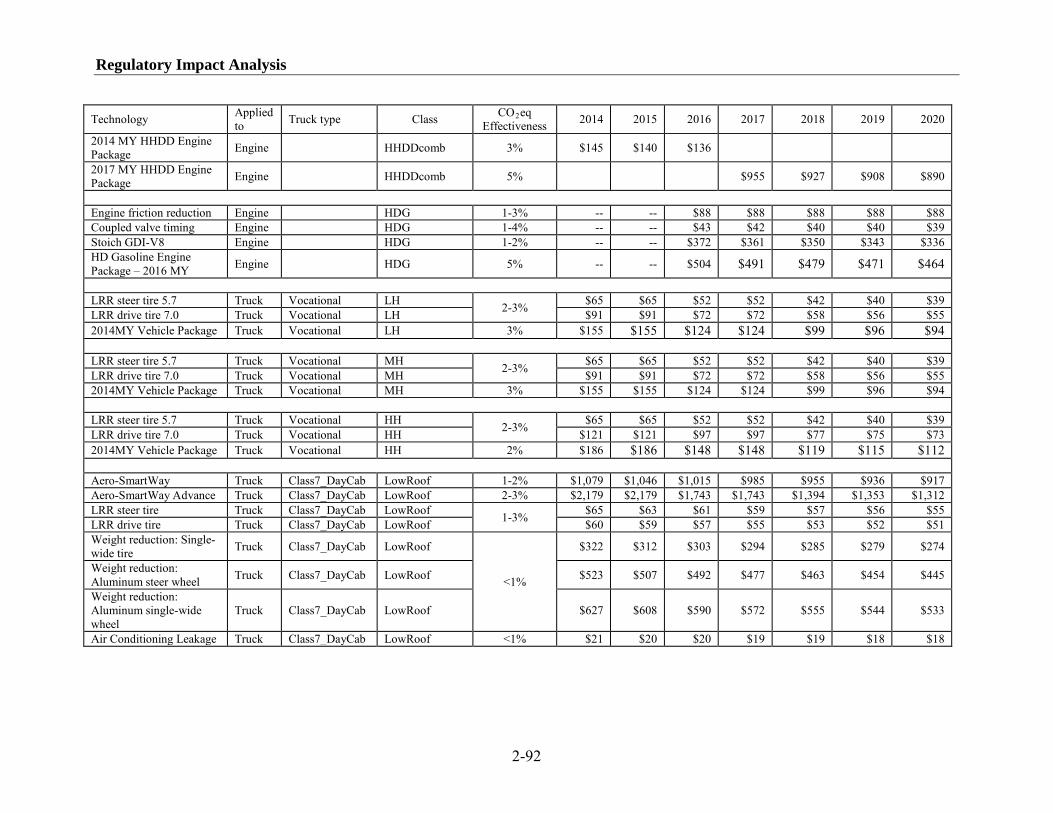
Regulatory Impact Analysis
2-92
Technology Applied to Truck type Class CO2 2014 eq
Effectiveness 2015 2016 2017 2018 2019 2020
2014 MY HHDD Engine Package Engine HHDDcomb 3% $145 $140 $136
2017 MY HHDD Engine Package Engine HHDDcomb 5% $955 $927 $908 $890
Engine friction reduction Engine HDG 1-3% -- -- $88 $88 $88 $88 $88 Coupled valve timing Engine HDG 1-4% -- -- $43 $42 $40 $40 $39 Stoich GDI-V8 Engine HDG 1-2% -- -- $372 $361 $350 $343 $336 HD Gasoline Engine Package – 2016 MY Engine HDG 5% -- -- $504 $491 $479 $471 $464
LRR steer tire 5.7 Truck Vocational LH 2-3% $65 $65 $52 $52 $42 $40 $39 LRR drive tire 7.0 Truck Vocational LH $91 $91 $72 $72 $58 $56 $55 2014MY Vehicle Package Truck Vocational LH 3% $155 $155 $124 $124 $99 $96 $94
LRR steer tire 5.7 Truck Vocational MH 2-3% $65 $65 $52 $52 $42 $40 $39 LRR drive tire 7.0 Truck Vocational MH $91 $91 $72 $72 $58 $56 $55 2014MY Vehicle Package Truck Vocational MH 3% $155 $155 $124 $124 $99 $96 $94
LRR steer tire 5.7 Truck Vocational HH 2-3% $65 $65 $52 $52 $42 $40 $39 LRR drive tire 7.0 Truck Vocational HH $121 $121 $97 $97 $77 $75 $73 2014MY Vehicle Package Truck Vocational HH 2% $186 $186 $148 $148 $119 $115 $112
Aero-SmartWay Truck Class7_DayCab LowRoof 1-2% $1,079 $1,046 $1,015 $985 $955 $936 $917 Aero-SmartWay Advance Truck Class7_DayCab LowRoof 2-3% $2,179 $2,179 $1,743 $1,743 $1,394 $1,353 $1,312 LRR steer tire Truck Class7_DayCab LowRoof 1-3% $65 $63 $61 $59 $57 $56 $55 LRR drive tire Truck Class7_DayCab LowRoof $60 $59 $57 $55 $53 $52 $51 Weight reduction: Single-wide tire Truck Class7_DayCab LowRoof
<1%
$322 $312 $303 $294 $285 $279 $274
Weight reduction: Aluminum steer wheel Truck Class7_DayCab LowRoof $523 $507 $492 $477 $463 $454 $445
Weight reduction: Aluminum single-wide wheel
Truck Class7_DayCab LowRoof $627 $608 $590 $572 $555 $544 $533
Air Conditioning Leakage Truck Class7_DayCab LowRoof <1% $21 $20 $20 $19 $19 $18 $18

Heavy Duty GHG and Fuel Efficiency Standards NPRM: Technologies, Cost, and Effectiveness
2-93
Technology Applied to Truck type Class CO2 2014 eq
Effectiveness 2015 2016 2017 2018 2019 2020
2014MY Vehicle PackageB Truck Class7_DayCab LowRoof 3-4% $2,593 $2,529 $2,379 $2,318 $2,189 $2,142 $2,097
Aero-SmartWay Truck Class7_DayCab HighRoof 2-4% $1,107 $1,074 $1,042 $1,011 $980 $961 $941 Aero-SmartWay Advance Truck Class7_DayCab HighRoof 3-5% $2,207 $2,207 $1,766 $1,766 $1,413 $1,370 $1,329 LRR steer tire Truck Class7_DayCab HighRoof 1-3% $65 $63 $61 $59 $57 $56 $55 LRR drive tire Truck Class7_DayCab HighRoof $60 $59 $57 $55 $53 $52 $51 Weight reduction: Single-wide tire Truck Class7_DayCab HighRoof
<1%
$322 $312 $303 $294 $285 $279 $274
Weight reduction: Aluminum steer wheel Truck Class7_DayCab HighRoof $523 $507 $492 $477 $463 $454 $445
Weight reduction: Aluminum single-wide wheel
Truck Class7_DayCab HighRoof $627 $608 $590 $572 $555 $544 $533
Air Conditioning Leakage Truck Class7_DayCab HighRoof <1% $21 $20 $20 $19 $19 $18 $18 2014MY Vehicle Package Truck Class7_DayCab HighRoof 6-7% $2,835 $2,763 $2,605 $2,537 $2,401 $2,350 $2,301
Aero-SmartWay Truck Class8_DayCab LowRoof 1-2% $1,079 $1,046 $1,015 $985 $955 $936 $917 Aero-SmartWay Advance Truck Class 8_DayCab LowRoof 2-3% $2,179 $2,179 $1,743 $1,743 $1,394 $1,353 $1,312 LRR steer tire Truck Class8_DayCab LowRoof 1-3% $65 $63 $61 $59 $57 $56 $55 LRR drive tire Truck Class8_DayCab LowRoof $121 $117 $114 $110 $107 $105 $103 Weight reduction: Single-wide tire Truck Class8_DayCab LowRoof
<1%
$644 $624 $606 $588 $570 $559 $547
Weight reduction: Aluminum steer wheel Truck Class8_DayCab LowRoof $523 $507 $492 $477 $463 $454 $445
Weight reduction: Aluminum single-wide wheel
Truck Class8_DayCab LowRoof $1,254 $1,216 $1,180 $1,144 $1,110 $1,088 $1,066
Air Conditioning Leakage Truck Class8_DayCab LowRoof <1% $21 $20 $20 $19 $19 $18 $18 2014MY Vehicle Package Truck Class8_DayCab LowRoof 3-4% $3,275 $3,176 $3,081 $2,989 $2,899 $2,841 $2,784
Aero-SmartWay Truck Class8_DayCab HighRoof 2-4% $1,107 $1,074 $1,042 $1,011 $980 $961 $941 Aero-SmartWay Advance Truck Class8_DayCab HighRoof 3-5% $2,207 $2,207 $1,766 $1,766 $1,413 $1,370 $1,329
B All vehicle package costs in the table include the proposed application rates of the individual technologies used to establish the proposed standards.
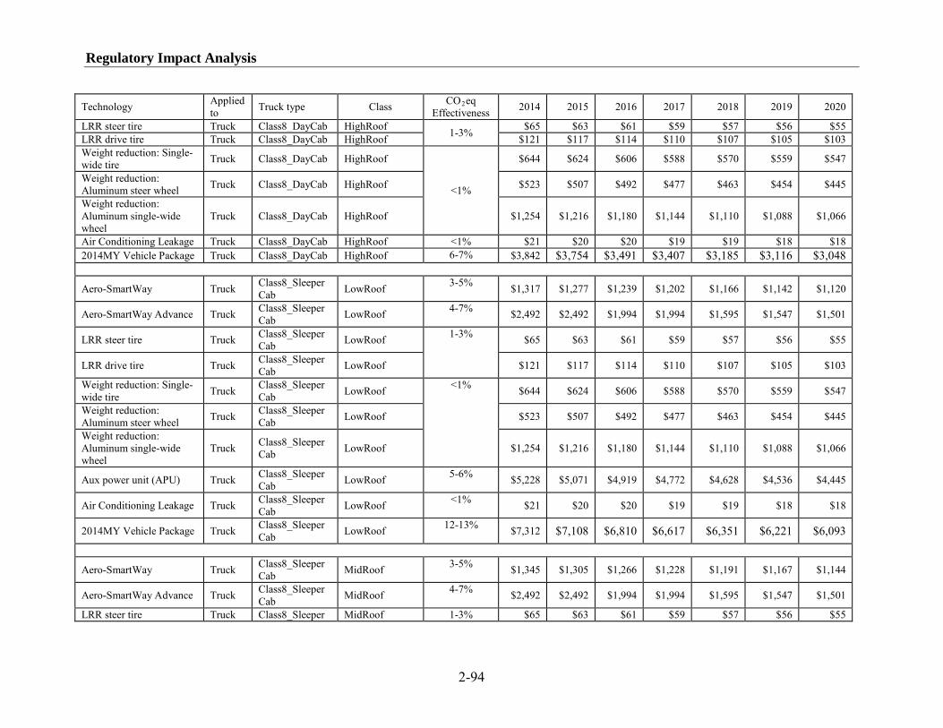
Regulatory Impact Analysis
2-94
Technology Applied to Truck type Class CO2 2014 eq
Effectiveness 2015 2016 2017 2018 2019 2020
LRR steer tire Truck Class8_DayCab HighRoof 1-3% $65 $63 $61 $59 $57 $56 $55 LRR drive tire Truck Class8_DayCab HighRoof $121 $117 $114 $110 $107 $105 $103 Weight reduction: Single-wide tire Truck Class8_DayCab HighRoof
<1%
$644 $624 $606 $588 $570 $559 $547
Weight reduction: Aluminum steer wheel Truck Class8_DayCab HighRoof $523 $507 $492 $477 $463 $454 $445
Weight reduction: Aluminum single-wide wheel
Truck Class8_DayCab HighRoof $1,254 $1,216 $1,180 $1,144 $1,110 $1,088 $1,066
Air Conditioning Leakage Truck Class8_DayCab HighRoof <1% $21 $20 $20 $19 $19 $18 $18 2014MY Vehicle Package Truck Class8_DayCab HighRoof 6-7% $3,842 $3,754 $3,491 $3,407 $3,185 $3,116 $3,048
Aero-SmartWay Truck Class8_SleeperCab LowRoof 3-5% $1,317 $1,277 $1,239 $1,202 $1,166 $1,142 $1,120
Aero-SmartWay Advance Truck Class8_SleeperCab LowRoof 4-7% $2,492 $2,492 $1,994 $1,994 $1,595 $1,547 $1,501
LRR steer tire Truck Class8_SleeperCab LowRoof 1-3% $65 $63 $61 $59 $57 $56 $55
LRR drive tire Truck Class8_SleeperCab LowRoof $121 $117 $114 $110 $107 $105 $103
Weight reduction: Single-wide tire Truck Class8_Sleeper
Cab LowRoof <1% $644 $624 $606 $588 $570 $559 $547
Weight reduction: Aluminum steer wheel Truck Class8_Sleeper
Cab LowRoof $523 $507 $492 $477 $463 $454 $445
Weight reduction: Aluminum single-wide wheel
Truck Class8_SleeperCab LowRoof $1,254 $1,216 $1,180 $1,144 $1,110 $1,088 $1,066
Aux power unit (APU) Truck Class8_SleeperCab LowRoof 5-6% $5,228 $5,071 $4,919 $4,772 $4,628 $4,536 $4,445
Air Conditioning Leakage Truck Class8_SleeperCab LowRoof <1% $21 $20 $20 $19 $19 $18 $18
2014MY Vehicle Package Truck Class8_SleeperCab LowRoof 12-13% $7,312 $7,108 $6,810 $6,617 $6,351 $6,221 $6,093
Aero-SmartWay Truck Class8_SleeperCab MidRoof 3-5% $1,345 $1,305 $1,266 $1,228 $1,191 $1,167 $1,144
Aero-SmartWay Advance Truck Class8_SleeperCab MidRoof 4-7% $2,492 $2,492 $1,994 $1,994 $1,595 $1,547 $1,501
LRR steer tire Truck Class8_Sleeper MidRoof 1-3% $65 $63 $61 $59 $57 $56 $55

Heavy Duty GHG and Fuel Efficiency Standards NPRM: Technologies, Cost, and Effectiveness
2-95
Technology Applied to Truck type Class CO2 2014 eq
Effectiveness 2015 2016 2017 2018 2019 2020
Cab
LRR drive tire Truck Class8_SleeperCab MidRoof $121 $117 $114 $110 $107 $105 $103
Weight reduction: Single-wide tire Truck Class8_Sleeper
Cab MidRoof <1% $644 $624 $606 $588 $570 $559 $547
Weight reduction: Aluminum steer wheel Truck Class8_Sleeper
Cab MidRoof $523 $507 $492 $477 $463 $454 $445
Weight reduction: Aluminum single-wide wheel
Truck Class8_SleeperCab MidRoof $1,254 $1,216 $1,180 $1,144 $1,110 $1,088 $1,066
Aux power unit (APU) Truck Class8_SleeperCab MidRoof 5-6% $5,228 $5,071 $4,919 $4,772 $4,628 $4,536 $4,445
Air Conditioning Leakage Truck Class8_SleeperCab MidRoof <1% $21 $20 $20 $19 $19 $18 $18
2014MY Vehicle Package Truck Class8_SleeperCab MidRoof 11-12% $7,438 $7,238 $6,893 $6,704 $6,402 $6,269 $6,139
Aero-SmartWay Truck Class8_SleeperCab HighRoof 3-5% $1,495 $1,450 $1,406 $1,364 $1,323 $1,297 $1,271
Aero-SmartWay Advance Truck Class8_SleeperCab HighRoof 4-7% $2,564 $2,564 $2,051 $2,051 $1,641 $1,591 $1,544
LRR steer tire Truck Class8_SleeperCab HighRoof 1-3% $65 $63 $61 $59 $57 $56 $55
LRR drive tire Truck Class8_SleeperCab HighRoof $121 $117 $114 $110 $107 $105 $103
Weight reduction: Single-wide tire Truck Class8_Sleeper
Cab HighRoof <1% $644 $624 $606 $588 $570 $559 $547
Weight reduction: Aluminum steer wheel Truck Class8_Sleeper
Cab HighRoof $523 $507 $492 $477 $463 $454 $445
Weight reduction: Aluminum single-wide wheel
Truck Class8_SleeperCab HighRoof $1,254 $1,216 $1,180 $1,144 $1,110 $1,088 $1,066
Aux power unit (APU) Truck Class8_SleeperCab HighRoof 5-6% $5,228 $5,071 $4,919 $4,772 $4,628 $4,536 $4,445
Air Conditioning Leakage Truck Class8_SleeperCab HighRoof <1% $21 $20 $20 $19 $19 $18 $18
2014MY Vehicle Package Truck Class8_SleeperCab HighRoof 15-16% $7,814 $7,587 $7,316 $7,103 $6,855 $6,716 $6,580

Regulatory Impact Analysis
2-96
Table 2-36 Technology Effectiveness and Costs, Inclusive of Markups, by Year for HD Diesel and Gasoline Pickup Trucks & Vans (2008$)
Technology Applied to CO2eq Effectiveness 2014 2015 2016 2017 2018 2019 2020
Low friction lubricants All 0-1% $4 $4 $4 $4 $4 $4 $4
Engine friction reduction
HD Gasoline 1-3% $108 $108 $108 $108 $108 $108 $108
Coupled cam phasing
HD Gasoline 1-4% $46 $44 $43 $43 $43 $43 $43
Cylinder deactivation
HD Gasoline 3-4% $193 $187 $182 $182 $182 $182 $182
Stoich GDI V8 HD Gasoline 1-2% $395 $384 $372 $372 $372 $372 $372
8sp AT (relative to 6sp AT) All 1.7% $231 $224 $218 $218 $218 $218 $218
Low RR Tires All 1-2% $6 $6 $6 $6 $6 $6 $6 Aero1 All 1-2% $54 $53 $51 $51 $51 $51 $51 Electric/Electro-hydraulic Power steering
All 1-2% $108 $104 $101 $101 $101 $101 $101
DSL engine improvements HD Diesel 4-6% $172 $167 $162 $157 $152 $148 $145
DSL aftertreatment improvements
HD Diesel 3-5% $110 $107 $104 $104 $104 $104 $104
Improved accessories HD Diesel 1-2% $88 $85 $82 $82 $82 $82 $82
Mass Reduction (5%)
2b HDGasoline 1.6% $462 $448 $435 $435 $435 $435 $435
Mass Reduction (5%)
2b HDDiesel 1.6% $544 $527 $511 $511 $511 $511 $511
Mass Reduction (5%)
3 HDGasoline 1.6% $513 $498 $483 $483 $483 $483 $483
Mass Reduction (5%) 3 HDDiesel 1.6% $576 $559 $542 $542 $542 $542 $542
Air Conditioning All 2% $21 $20 $20 $19 $19 $18 $18
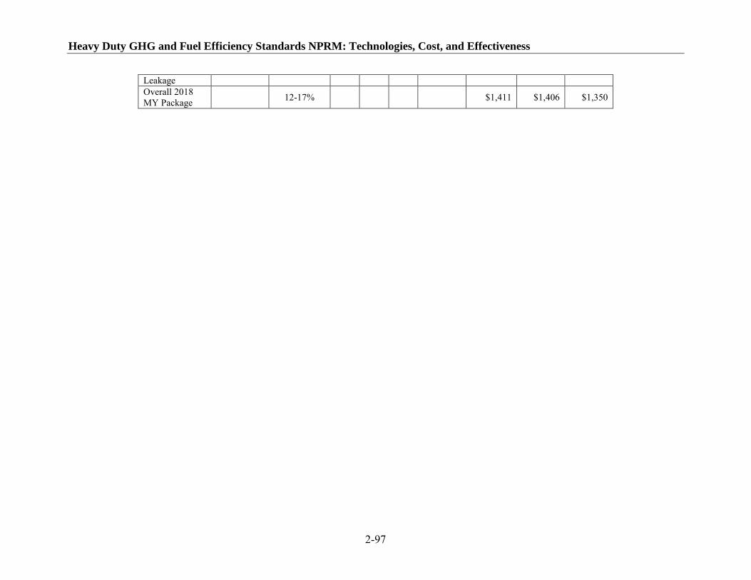
Heavy Duty GHG and Fuel Efficiency Standards NPRM: Technologies, Cost, and Effectiveness
2-97
Leakage Overall 2018 MY Package 12-17% $1,411 $1,406 $1,350

Regulatory Impact Analysis
2-98
References
1 National Academy of Science. Technologies and Approaches to Reducing the Fuel Consumption of Medium- and Heavy-Duty Vehicles. March 2010. 2 TIAX, LLC. Assessment of Fuel Economy Technologies for Medium- and Heavy-Duty Vehicles. November 2009. 3 U.S. EPA. EPA Lumped Parameter Model HD Version 1.0.0.5, 2010. Docket #EPA-HQ-OAR-2010-0162. 4 NESCCAF, ICCT, Southwest Research Institute, and TIAX. Reducing Heavy-Duty Long Haul Combination Truck Fuel Consumption and CO2 Emissions. October 2009. 5 ICF International. Investigation of Costs for Strategies to Reduce Greenhouse Gas Emissions for Heavy-Duty On-Road Vehicles. July 2010. Docket Identification Number EPA-HQ-OAR-2010-0162-0044. 6 Revenue = Direct Costs + Indirect Costs + Net Income 7 RTI International. Heavy Duty Truck Retail Price Equivalent and Indirect Cost Multipliers. July 2010.
8 See “Learning Curves in Manufacturing”, L. Argote and D. Epple, Science, Volume 247; “Toward Cost Buy down Via Learning-by-Doing for Environmental Energy Technologies, R. Williams, Princeton University, Workshop on Learning-by-Doing in Energy Technologies, June 2003; “Industry Learning Environments and the Heterogeneity of Firm Performance, N. Balasubramanian and M. Lieberman, UCLA Anderson School of Management, December 2006, Discussion Papers, Center for Economic Studies, Washington DC.
9 U.S. EPA and NHTSA, “Final Rulemaking to Establish Light-Duty Vehicle Greenhouse Gas Emission Standards and Corporate Average Fuel Economy Standards – Joint Technical Support Document,” 2010. Last viewed on June 3, 2010 at http://www.epa.gov/otaq/climate/regulations/420r10901.pdf 10 Note that throughout the cost estimates for this HD analysis, the agencies have used slightly higher markups than those used in the 2010-2016 light-duty FRM. The new, slightly higher ICMs include return on capital of roughly 6 percent, a factor that was not included in the light-duty analysis. 11 Note that the costs developed for low friction lubes for this analysis reflect the costs associated with any engine changes that would be required as well as any durability testing that may be required. 12 U.S. EPA and NHTSA, “Final Rulemaking to Establish Light-Duty Vehicle Greenhouse Gas Emission Standards and Corporate Average Fuel Economy Standards – Joint Technical Support Document,” 2010. Last viewed on June 3, 2010 at http://www.epa.gov/otaq/climate/regulations/420r10901.pdf 13 Note that throughout the cost estimates for this HD analysis, the agencies have used slightly higher markups than those used in the 2010-2016 light-duty FRM. The new, slightly higher ICMs include return on capital of roughly 6 percent, a factor that was not included in the light-duty analysis. 14 Note that the costs developed for low friction lubes for this analysis reflect the costs associated with any engine changes that would be required as well as any durability testing that may be required. 15 TIAX. Assessment of Fuel Economy Technologies for Medium- and Heavy- Duty Vehicles, Final Report, Nov. 19, 2009, pg 4-15. 16 Stanton, Donald. “Enabling High Efficiency Clean Combustion.” 2009 Semi-Mega Merit Review of the Department of Energy. May 21, 2009. Last accessed on August 25, 2010 at http://www1.eere.energy.gov/vehiclesandfuels/pdfs/merit_review_2009/advanced_combustion/ace_40_stanton.pdf. 17 Stanton, Donald. “Enabling High Efficiency Clean Combustion.” 2009 Semi-Mega Merit Review of the Department of Energy. May 21, 2009. Last accessed on August 25, 2010 at http://www1.eere.energy.gov/vehiclesandfuels/pdfs/merit_review_2009/advanced_combustion/ace_40_stanton.pdf.

Heavy Duty GHG and Fuel Efficiency Standards NPRM: Technologies, Cost, and Effectiveness
2-99
18 “Tires and Passenger Vehicle Fuel Economy,” Transportation Research Board Special Report 286, National Research Council of the National Academies, 2006, Docket EPA-HQ-OAR-2009-0472-0146. 19 U.S. EPA and NHTSA, “Final Rulemaking to Establish Light-Duty Vehicle Greenhouse Gas Emission Standards and Corporate Average Fuel Economy Standards – Joint Technical Support Document,” 2010. Last viewed on June 3, 2010 at http://www.epa.gov/otaq/climate/regulations/420r10901.pdf 20 U.S.EPA, EPA Lumped Parameter Model HD Version 1.0.0.5, 2010. Docket #EPA-HQ-OAR-2010-0162. 21 Stanton, Donald. “Enabling High Efficiency Clean Combustion.” 2009 Semi-Mega Merit Review of the Department of Energy. May 21, 2009. Last accessed on August 25, 2010 at http://www1.eere.energy.gov/vehiclesandfuels/pdfs/merit_review_2009/advanced_combustion/ace_40_stanton.pdf. 22 Zhang, H. Heavy Truck Engine Development & HECC. 2009 DOE Semi-Mega Merit Review, May 21, 2009. Last accessed on August 25, 2010 at http://www1.eere.energy.gov/vehiclesandfuels/pdfs/merit_review_2009/advanced_combustion/ace_42_zhang.pdf
23 NAS Report. 2010. Pages 53-54.
24 NAS Report. 2010. Page 54.
25 TIAX Report. 2009. Page 3-5.
26 NAS Report. 2010. Page 54.
27 Vuk, C. “Electric Turbo Compounding…A Technology Who’s Time Has Come.” 2006 DEER Conference. Last accessed on August 25, 2010 at http://www1.eere.energy.gov/vehiclesandfuels/pdfs/deer_2006/session6/2006_deer_vuk.pdf
28 TIAX, Nov. 19, 2009, page 4-15.
29 Zhang, H. “High Efficiency Clean Combustion for Heavy-Duty Engine.” August 6, 2008 presentation to DEER Conference. Last accessed on August 25, 2010 at http://www1.eere.energy.gov/vehiclesandfuels/pdfs/deer_2008/session5/deer08_zhang.pdf
30 NAS Report. 2010. Page 57.
31 NAS Report. 2010. Page 57. 32 Assumes travel on level road at 65 MPH. (21st Century Truck Partnership Roadmap and Technical White Papers, December 2006. U.S. Department of Energy, Energy Efficiency and Renewable Energy Program. 21CTP-003. p. 36.) 33 Reducing Heavy-Duty Long Haul Combination Truck Fuel Consumption and CO2 Emissions, ICCT, October 2009 34 SAE 2006-01-3456 35 U.S. EPA. Heavy-Duty Coastdown Test Procedure Development. Docket # EPA-HQ-OAR-2010-0162-0144. 36 ICF. Investigation of Costs for Strategies to Reduce Greenhouse Gas Emissions fro Heavy-Duty On-Road Vehicles. July 2010. Docket Identification Number EPA-HQ-OAR-2010-0162-0044. 37 21st Century Truck Partnership, “Roadmap and technical White Papers”, U.S. Department of Energy, Technical paper: 21CTP-0003, December 2006.

Regulatory Impact Analysis
2-100
38 “Tires & Truck Fuel Economy,” A New Perspective. Bridgestone Firestone, North American Tire, LLC, Special Edition Four, 2008. 39 “Michelin’s Green Meters,” Press Kit, October, 30, 2007. http://www.michelin-green-meter.com/main.php?cLang=en (Complete Press File, Viewed March 6, 2010) 40 “Modeling of Fuel Consumption for Heavy-Duty Trucks and the Impact of Tire Rolling Resistance,” Tim J. LaClair, Russell Truemner, SAE International, 2005-01-3550, 2005. 41 “Factors Affecting Truck Fuel Economy,” Goodyear, Radial Truck and Retread Service Manual. Accessed February 16, 2010 at http://www.goodyear.com/truck/pdf/radialretserv/Retread_S9_V.pdf. 42 “Tire Rolling Resistance, Its Impact on Fuel Economy, and Measurement Standards,” Presentation by Tim J. LaClair of Michelin Americas Research & Development Corp. to the California Energy Commission, 2002. 43 “Technology Roadmap for the 21st Century Truck Program. A Government-Industry Partnership,” U.S. Department of Energy, 21CT-001, December 2000. 44 “Energy Efficiency Strategies for Freight Trucking: Potential Impact on Fuel Use and Greenhouse Gas Emissions,” J. Ang-Olson, W. Schroer, Transportation Research Record: Journal of the Transportation Research Board, 2002(1815):11-18. 45 “Effect of Single Wide Tires and Trailer Aerodynamics on Fuel Economy and NOx Emissions of Class 8 Line-Haul Tractor-Trailer,” J. Bachman, A. Erb, C. Bynum, U.S. Environmental Protection Agency, SAE International, Paper Number 05CV-45, 2005. 46 “Class 8 Heavy Truck Duty Cycle Project Final Report,” U.S. Department of Energy, Oak Ridge National Laboratory, ORNL/TM-2008/122, p. 21, December 2008. Accessed January 19, 2010 at http://cta.ornl.gov/cta/Publications/Reports/ORNL_TM_2008-122.pdf. 47 “Are Ultra-Wide, Ultra-Low Aspect Ratio Tires the Next Big Thing?” K. Rohlwing, Today’s Tire Industry, Vol. 1, Issue 1, July/August, July 2003. 48 “New Generation Wide Base Single Tires,” American Trucking Association, White paper presented at the International Workshop on the use of wide tires sponsored by Federal Highway Administration, Turner-Fairbank Highway Research Center, October 25-26, 2007, Revision 9, December 21, 2007, Accessed on February 3, 2010 at http://www.arc.unr.edu/Workshops/Wide_Tires/Wide_Base_Summary-v9-ATA-whitepaper.pdf 49 “Recommended Practice: Guidelines for Outset Wide Base Wheels for Drive, Trailer and Auxiliary Axle Applications (Draft),” Technology and Maintenance Council, Council of American Trucking Associations, circulated September 28, 2009. 50 ICF. Investigation of Costs for Strategies to Reduce Greenhouse Gas Emissions fro Heavy-Duty On-Road Vehicles. July 2010. Docket Identification Number EPA-HQ-OAR-2010-0162-0044. 51 “Buses & Retread Tires,” The Tire Retread & Repair Information Bureau, Pacific Grove, Ca., Accessed on January 27, 2010 at http://www.retread.org/packet/index.cfm/ID/284.htm. 52 “What are Retreaders Doing to Improve Fuel Efficiency?” H. Inman, Tire Review, December 11, 2006, Accessed on February 18, 2010 at http://www.tirereview.com/Article/59777/what_are_retreaders_doing_to_improve_fuel_efficiency.aspx. 53 “Better Fuel Economy? Start with a Strong Tire Program,” H. Inman, Fleet & Tire 2006, Tire Review, December 11, 2006, Accessed on February 18, 2010 at http://www.tirereview.com/Article/59776/better_fuel_economy_start_with_a_strong_tire_program.aspx. 54 “SmartWay Transport Partnership: Innovative Carrier Strategies”, February 2004, EPA420-F-04-005, Accessed on the Internet on January 18, 2010 at: http://www.epa.gov/smartway/transport/what-smartway/carrier-strategies.htm#weight.

Heavy Duty GHG and Fuel Efficiency Standards NPRM: Technologies, Cost, and Effectiveness
2-101
55 “Energy Savings through Increased Fuel Economy for Heavy Duty Trucks”, Therese Langer, American Council for an Energy-Efficient Economy prepared for the National Commission on Energy Policy, February 11, 2004. 56 “The Potential Effect of Future Energy-Efficiency and Emissions-Improving Technologies on Fuel Consumption of Heavy Trucks”, Argonne National Laboratory, Technical Report ANL/ESD/02-4, August 2002. 57 U.S. EPA. http://www.epa.gov/smartway/documents/weightreduction.pdf 58 U.S. EPA. http://www.epa.gov/smartway/documents/weightreduction.pdf 59 Gaines, L. and D. Santini. Argonne National Laboratory, Economic Analysis of Commercial Idling Reduction Technologies 60 Gaines, L., A. Vyas, J. Anderson. Estimation of Fuel Use by Idling Commercial Trucks. 2006. Page 9. 61 Gaines, L., A. Vyas, J. Anderson. Estimation of Fuel Use by Idling Commercial Trucks. 2006. Page 7. 62 NAS Study. 2010. Page 122 says the best in class APU consumes 0.18 gallon per hour. 63 American Trucking Association. Last viewed on January 29, 2010 at http://www.trucksdeliver.org/recommendations/speed-limits.html 64 U.S. EPA SmartWay Transport Partnership. Last viewed on January 28, 2010 at http://www.epa.gov/smartway/transport/documents/tech/reducedspeed.pdf 65 Department for Transport, Vehicle and Operator Services Agency. Last viewed on January 6, 2010 at http://www.dft.gov.uk/vosa/newsandevents/pressreleases/2006pressreleases/28-12-06speedlimiterlegislation.htm 66 Transport Canada. Summary Report – Assessment of a Heavy Truck Speed Limiter Requirement in Canada. Last viewed on January 6, 2010 at http://www.tc.gc.ca/eng/roadsafety/tp-tp14808-menu-370.htm 67 Transport Canada. Summary Report – Assessment of a Heavy-Truck Speed Limiter Requirement in Canada. 68 “Assessment of Fuel Economy Technologies for Medium- and Heavy-Duty Vehicles”, TIAX LLC, November 19, 2009. Page 4-98. 69 “Assessment of Fuel Economy Technologies for Medium- and Heavy-Duty Vehicles”, TIAX LLC, November 19, 2009. Page 4-98. 70 US Environmental Protection Agency's SmartWay Transport Partnership July 2010 e-update accessed July 16, 2010, from http://www.epa.gov/smartwaylogistics/newsroom/documents/e-update-july-10.pdf 71 TIAX. Assessment of Fuel Economy Technologies for Medium- and Heavy-Duty Vehicles. November 2009. Page 4-40. 72 U.S. Department of Energy. Transportation Energy Data Book, Edition 28-2009. Table 5.7.
73 As explained further in Section V below, EPA would use these inputs in GEM even for engines electing to use the alternative engine standard.
74 US Environmental Protection Agency's SmartWay Transport Partnership July 2010 e-update accessed July 16, 2010, from http://www.epa.gov/smartwaylogistics/newsroom/documents/e-update-july-10.pdf 75 Rubber Manufacturers Association. Presentation to California Air Resource Board. June 2009. Last viewed at http://www.rma.org/rma_resources/government_affairs/federal_issues/RMA%20COMMENTS%20APPENDIX%201%20-%20ENVIRON%20Report%20-%20Data%20Analysis.pdf

Regulatory Impact Analysis
2-102
76 Kargul, J. J., 2010, "Clean Automotive Technology. Cost-Effective Solutions for a Petroleum and Carbon Constrained World," Presentation made to National Academy of Sciences, Review of 21st Century Truck Program, September 8, 2010
77 “Best practices Guidebook for Greenhouse Gas Reductions in Freight Transportation”, H. Christopher Fey, Po-Yao Kuo, North Carolina State University prepared for the U.S. Department of Transportation, October 4, 2007. 78 “Reducing Heavy-Duty long haul Combination Truck Fuel Consumption and CO2 Emissions”, NESCCAF, ICCT, SwRI, TIAX LLC, October 2009.
79 The U.S. EPA has reclamation requirements for refrigerants in place under Title VI of the Clean Air Act.
80 The global warming potentials (GWP) used in the NPRM analysis are consistent with Intergovernmental Panel on Climate Change (IPCC) Fourth Assessment Report (AR4). At this time, the IPCC Second Assessment Report (SAR) global warming potential values have been agreed upon as the official U.S. framework for addressing climate change. The IPCC SAR GWP values are used in the official U.S. greenhouse gas inventory submission to the climate change framework. When inventories are recalculated for the final rule, changes in GWP used may lead to adjustments. 81 Schwarz, W., Harnisch, J. 2003. “Establishing Leakage Rates of Mobile Air Conditioners.” Prepared for the European Commission (DG Environment), Doc B4-3040/2002/337136/MAR/C1. 82 Vincent, R., Cleary, K., Ayala, A., Corey, R. 2004. “Emissions of HFC-134a from Light-Duty Vehicles in California.” SAE 2004-01-2256. 83 The Minnesota refrigerant leakage data can be found at http://www.pca.state.mn.us/climatechange/mobileair.html#leakdata. 84 Society of Automotive Engineers, “IMAC Team 1 – Refrigerant Leakage Reduction, Final Report to Sponsors,” 2006. 85 Society of Automotive Engineers Surface Vehicle Standard J2727, issued August 2008, http://www.sae.org. 86 U.S. Department of Transportation, Federal Highway Administration. Federal Highway Statistics. “Trailer and Semitrailer Registrations – 2008” Table MV-11 located at www.fhwa.dot.gov/policyinformation/statistics/2008/mv11.cfm 87 The International Council on Clean Transportation. Heavy Duty Vehicle Market Analysis. May 2009. Table 88Trailer Body Builders. Last viewed on August 18, 2010 at http://trailer-bodybuilders.com/trailer-output/output/2008_trailer_output_table/ 89 ICF. Investigation of Costs for Strategies to Reduce Greenhouse Gas Emissions fro Heavy-Duty On-Road Vehicles. July 2010. Docket Identification Number EPA-HQ-OAR-2010-0162-0044. 90 “Review of Low Carbon Technologies for Heavy Goods Vehicles – Annex 1”, Ricardo prepared for Department of Transport, Technology Paper RD.09/182601.7, Jun 2009 91 U.S. Environmental Protection Agency Office of Transportation and Air Quality SmartWay Transport Partnership, A Glance at Clean Freight Strategies: Drivers Training EPA 420-F-04-008; February 2004. 92 Ibid. 93 National Research Council, Technologies and Approaches to Reducing the Fuel Consumption of Medium- and Heavy-Duty Vehicles, Committee to Assess Fuel Economy Technologies for Medium- and Heavy-Duty Vehicles; Washington, DC, National Academies Press, 2010. 94 Information from US EPA review of 2009 SmartWay Excellence Awards applications.

Heavy Duty GHG and Fuel Efficiency Standards NPRM: Technologies, Cost, and Effectiveness
2-103
95 U.S. Environmental Protection Agency Office of Transportation and Air Quality SmartWay Transport Partnership, A Glance at Clean Freight Strategies: Drivers Training EPA 420-F-04-008; February 2004. 96 National Research Council, Technologies and Approaches to Reducing the Fuel Consumption of Medium- and Heavy-Duty Vehicles, Committee to Assess Fuel Economy Technologies for Medium- and Heavy-Duty Vehicles; Washington, DC, National Academies Press, 2010. 97 Technology and Maintenance Council of the American Trucking Associations, Tire Air Pressure Study, Tire Debris Prevention Task Force S.2 Tire & Wheel Study Group; May 2002. 98 National Research Council, Technologies and Approaches to Reducing the Fuel Consumption of Medium- and Heavy-Duty Vehicles, Committee to Assess Fuel Economy Technologies for Medium- and Heavy-Duty Vehicles; Washington, DC, National Academies Press, 2010. 99 U.S. Environmental Protection Agency Office of Transportation and Air Quality SmartWay Transport Partnership, A Glance at Clean Freight Strategies: Automatic Tire Inflation Systems EPA 420-F-04-0010; February 2004. 100 National Research Council, Technologies and Approaches to Reducing the Fuel Consumption of Medium- and Heavy-Duty Vehicles, Committee to Assess Fuel Economy Technologies for Medium- and Heavy-Duty Vehicles; Washington, DC, National Academies Press, 2010. 101 Ibid. 102 “Comprehensive Truck Weight and Size Study: Summary Report,” U.S. DOT Federal Highway Traffic Administration, August 2000. 103 “Comprehensive Truck Weight and Size Study: Summary Report,” U.S. DOT Federal Highway Traffic Administration, August 2000. 104 “Comprehensive Truck Weight and Size Study: Summary Report,” U.S. DOT Federal Highway Traffic Administration, August 2000. 105 National Research Council, Technologies and Approaches to Reducing the Fuel Consumption of Medium- and Heavy-Duty Vehicles, Committee to Assess Fuel Economy Technologies for Medium- and Heavy-Duty Vehicles; Washington, DC, National Academies Press, 2010.

Heavy-Duty GHG and Fuel Efficiency Standards NPRM: Test Procedures
3-1
Chapter 3: Test Procedures Test procedures are a crucial aspect of the proposed heavy-duty vehicle GHG and fuel
consumption program. The proposed rulemaking is establishing several new test procedures for both engine and vehicle compliance. This chapter will describe the development process for the test procedures being proposed, including the assessment of engines, aerodynamics, rolling resistance, chassis dynamometer testing, and drive cycles.
3.1 Heavy-Duty Engine Test Procedure
The agencies are proposing to control heavy-duty engine fuel consumption and greenhouse gas emissions through the use of engine certification. The proposed program will mirror existing engine regulations for the control of non-GHG pollutants in many aspects. The following sections provide an overview of the proposed test procedures.
3.1.1 Existing Regulation Reference
Heavy-duty engines currently are certified for non-GHG pollutants using test procedures developed by EPA. The Heavy-Duty Federal Test Procedure is a transient test consisting of second-by-second sequences of engine speed and torque pairs with values given in normalized percent of maximum form. The cycle was computer generated from a dataset of 88 heavy-duty trucks in urban operation in New York and Los Angeles. These procedures are well-defined and we believe appropriate also for the assessment of GHG emissions. EPA is concerned that we maintain a regulatory relationship between the non-GHG emissions and GHG emissions, especially for control of CO2 and NOx
For 2007 and later Heavy-Duty engines, Parts 86 – “Control of Emissions from New and In-Use Highway Vehicles and Engines” and 1065 – “Engine Testing Procedures” detail the certification process. Part 86.007-11 defines the standard settings of Oxides of Nitrogen, Non-Methane Hydrocarbons, Carbon Monoxide, and Particulate. The duty cycles are defined in Part 86. The Federal Test Procedure engine test cycle is defined in Part 86 Appendix I. The Supplemental Emissions Test engine cycle is defined in §86.1360-2007(b). All emission measurements and calculations are defined in Part 1065, with exceptions as noted in §86.007-11. The data requirements are defined in § 86.001-23 and 1065.695.
. Therefore, we are proposing to use the same test procedures.
The procedure for CO2 measurement is presented in §1065.250. For measurement of CH4 refer to §1065.260. For measurement of N2O refer to §1065.275. We recommend that you use an analyzer that meets performance specifications shown in Table 1 of §1065.205. Note that your system must meet the linearity verification of §1065.307. To calculate the brake specific mass emissions for CO2, CH4 and N2O refer to §1065.650. For CH4 refer to §1065.660(a) to calculate the contamination correction.

Draft Regulatory Impact Analysis
3-2
3.1.2 Engine Dynamometer Test Procedure Modifications
3.1.2.1 Fuel Consumption Calculation
EPA and NHTSA propose to calculate fuel consumption, as defined as gallons per brake horsepower-hour, from the CO2 measurement. The agencies are proposing that manufacturers use 8,887 gram of CO2 per gallon of gasoline and 10,180 g CO2
3.1.2.2 N
per gallon of diesel fuel.
2
EPA proposes that manufacturers would need to submit measurements of N
O Measurement
2O to be able to apply for a certificate of conformity with the N2O standard. Engine emissions regulations do not currently require testing for N2O, and most test facilities do not have equipment for its measurement. Manufacturers without this capability would need to acquire and install appropriate measurement equipment. For use commencing with MY 2015 engines and vehicles, EPA is proposing four N2
3.1.2.3 CO
O measurement methods, all of which are commercially available today. EPA expects that most manufacturers would use photo-acoustic measurement equipment, which the Agency estimates would result in a one-time cost of about $50,000 for each test cell that would need to be upgraded.
2
EPA and NHTSA evaluated two means to handle the CO
Measurement Variability
2
The agencies are proposing to take an approach where manufacturers are allowed to determine their own compliance margin, but it must be at least two percent to account for the test-to-test variation. The agencies developed the two percent threshold based on CO
and fuel consumption measurement variability. The first is to use an approach similar to the LD GHG and Fuel Economy program where the agencies adopted a compliance factor that is applied to the measured value. The second is an approach where the standard is set as a not to exceed standard. Manufacturers set a design target set sufficiently below the standard to account for production variability and deterioration.
2 measurement variability from several test programs. The programs include internal EPA round-robin testing, ACES1, and the Gaseous MA program.2 Table 3-1 summarizes the results from each of these programs.
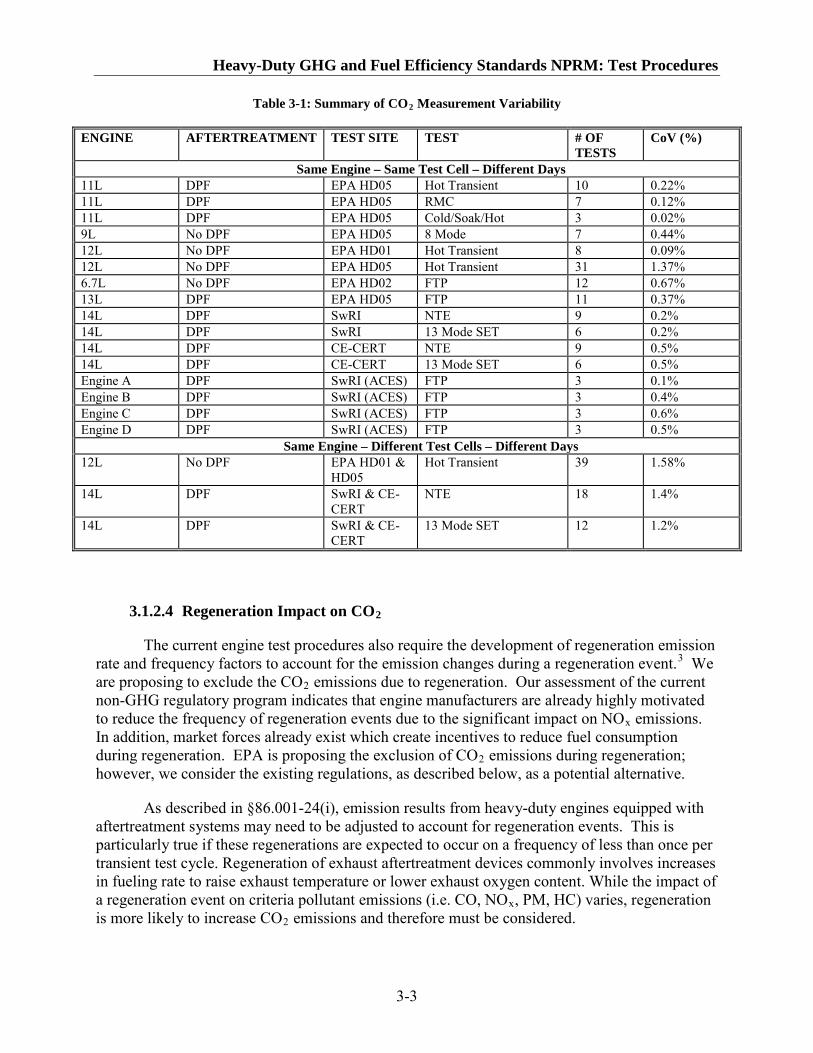
Heavy-Duty GHG and Fuel Efficiency Standards NPRM: Test Procedures
3-3
Table 3-1: Summary of CO2
ENGINE
Measurement Variability
AFTERTREATMENT TEST SITE TEST # OF TESTS
CoV (%)
Same Engine – Same Test Cell – Different Days 11L DPF EPA HD05 Hot Transient 10 0.22% 11L DPF EPA HD05 RMC 7 0.12% 11L DPF EPA HD05 Cold/Soak/Hot 3 0.02% 9L No DPF EPA HD05 8 Mode 7 0.44% 12L No DPF EPA HD01 Hot Transient 8 0.09% 12L No DPF EPA HD05 Hot Transient 31 1.37% 6.7L No DPF EPA HD02 FTP 12 0.67% 13L DPF EPA HD05 FTP 11 0.37% 14L DPF SwRI NTE 9 0.2% 14L DPF SwRI 13 Mode SET 6 0.2% 14L DPF CE-CERT NTE 9 0.5% 14L DPF CE-CERT 13 Mode SET 6 0.5% Engine A DPF SwRI (ACES) FTP 3 0.1% Engine B DPF SwRI (ACES) FTP 3 0.4% Engine C DPF SwRI (ACES) FTP 3 0.6% Engine D DPF SwRI (ACES) FTP 3 0.5%
Same Engine – Different Test Cells – Different Days 12L No DPF EPA HD01 &
HD05 Hot Transient 39 1.58%
14L DPF SwRI & CE-CERT
NTE 18 1.4%
14L DPF SwRI & CE-CERT
13 Mode SET 12 1.2%
3.1.2.4 Regeneration Impact on CO2
The current engine test procedures also require the development of regeneration emission rate and frequency factors to account for the emission changes during a regeneration event.
3 We are proposing to exclude the CO2 emissions due to regeneration. Our assessment of the current non-GHG regulatory program indicates that engine manufacturers are already highly motivated to reduce the frequency of regeneration events due to the significant impact on NOx emissions. In addition, market forces already exist which create incentives to reduce fuel consumption during regeneration. EPA is proposing the exclusion of CO2
As described in §86.001-24(i), emission results from heavy-duty engines equipped with aftertreatment systems may need to be adjusted to account for regeneration events. This is particularly true if these regenerations are expected to occur on a frequency of less than once per transient test cycle. Regeneration of exhaust aftertreatment devices commonly involves increases in fueling rate to raise exhaust temperature or lower exhaust oxygen content. While the impact of a regeneration event on criteria pollutant emissions (i.e. CO, NO
emissions during regeneration; however, we consider the existing regulations, as described below, as a potential alternative.
x, PM, HC) varies, regeneration is more likely to increase CO2 emissions and therefore must be considered.

Draft Regulatory Impact Analysis
3-4
The current regulations outline a method of accounting for changes in emissions due to regeneration events (§86.001-24(i)(1)-(i)(5)). This method involves developing downward and upward adjustment factors (D/UAFs) meant to characterize emissions with and without (respectively) a regeneration event. Combined with a frequency factor (F), characterizing the frequency at which regeneration occurs, these adjustments are applied to the final emission test results. Use of this procedure to account for changes in CO2 emissions during regeneration appears to be a practical, well accepted, and accurate method for certification. Any increases (or decreases) in CO2
3.1.2.5 Fuel Heating Value Correction
due to regeneration would be captured in the adjustment factors and final emission results could be corrected accordingly.
The agencies collected baseline CO2
The existing regulations correct for gasoline fuel properties, as described in Part 86. The same correction can be used for the testing of complete pickup trucks and vans with gasoline fueled engines.
performance of diesel engines from testing which used fuels with similar properties. The agencies are proposing a fuel-specific correction factor for the fuel’s energy content in case this changes in the future. The agencies found the average energy content of the diesel fuel used at EPA’s National Vehicle Fuel and Emissions Laboratory was 21,200 BTU per pound of carbon. This value is determined by dividing the Net Heating Value (BTU per pound) by the carbon weight fraction of the fuel used in testing.
The agencies are not proposing fuel corrections for alcohols because the fuel chemistry is homogeneous. The agencies are proposing a fuel correction for natural gas.
3.1.2.6 Multiple Fuel Maps
Modern heavy-duty engines may have multiple fuel maps, commonly meant to improve performance or fuel economy under certain operating conditions. CO2 emissions can also be different depending on which map is tested, so it is important to specify a procedure to properly deal with engines with multiple fuel maps. Consistent with criteria-pollutant emissions certification, engine manufacturers should submit CO2
3.1.3 Engine Family Definition and Test Engine Selection
data from all fuel maps on a given test engine. This includes fuel map information as well as the conditions under which a given fuel map is used (i.e. transmission gear, vehicle speed, etc).
3.1.3.1 Criteria for Engine Families
The current regulations outline the criteria for grouping engine models into engine families sharing similar emission characteristics. A few of these defining criteria include bore-center dimensions, cylinder block configuration, valve configuration, and combustion cycle; a comprehensive list can be found in §86.096-24(a)(2). While this set of criteria was developed with criteria pollutant emissions in mind, similar effects on CO2 emissions can be expected. For this reason, this methodology should continue to be followed when considering CO2 emissions.

Heavy-Duty GHG and Fuel Efficiency Standards NPRM: Test Procedures
3-5
3.1.3.2 Emissions Test Engine
Manufacturers must select at least one engine per engine family for emission testing. The methodology for selecting the test engine(s) should be consistent with §86.096-24(b)(2) (for heavy-duty Otto cycle engines) and §86.096-24(b)(3) (for heavy-duty diesel engines). An inherent characteristic of these methodologies is selecting the engine with the highest fuel feed per stroke (primarily at the speed of maximum rated torque and secondarily at rated speed) as the test engine, as this is expected to produce the worst-case criteria pollutant emissions. CO2 emissions are expected to scale well with fuel feed in a given engine family and therefore work-based CO2
3.2 Aerodynamic Assessment
measurements are expected to be less sensitive to the specific engine model selected than criteria pollutant emissions. To be consistent however, it is recommended that the same methodology continue to be used for selecting test engines.
The aerodynamics of a Class 7/8 combination tractor is dependent on many factors, including the tractor design, trailer design, gap between the tractor and trailer, vehicle speed, wind speed, and many others. We believe that to fairly assess the aerodynamics of combination tractors certain aspects of the truck need to be defined, including the trailer, location of payload, and tractor-trailer gap.
3.2.1 Standardized Trailer Definition
We are proposing to use a model input reflecting a standardized trailer for each subcategory of the Class 7/8 tractor subcategories based on tractor roof height. High roof tractors are designed to optimally pull box trailers. The height of the roof fairing is designed to minimize the height differential between the tractor and typical trailer to reduce the air flow disruption. Low roof tractors are designed to carry flatbed or low-boy trailers. Mid roof tractors are designed to carry tanker and bulk carrier trailers. High roof tractors are designed to optimally pull box trailers. However, we recognize that during actual operation tractors sometimes pull trailers that do not provide the optimal roof height that matches the tractor. In order to assess how often truck and trailer mismatches are found in operation, EPA conducted a study based on observations of traffic across the U.S.4
Section 1037.510 prescribes the proposed standardized trailer for each tractor subcategory (low, mid, and high roof) including trailer dimensions and tractor-trailer gap.
Data was gathered on over 4,000 tractor-trailer combinations using 33 live traffic cameras in 22 states across the United States. Approximately 95% of trucks were “matched” per our definition (e.g. box trailers were pulled by high roof tractors and flatbed trailers were pulled with low roof tractors). The amount of mismatch varied depending on the type of location. Over 99% of the tractors were observed to be in matched configuration in Indiana at the I-80/I-94/I-65 interchange, which is representative of long-haul operation. On the other hand, only about 90% of the tractors were matched with the appropriate trailer in metro New York City, where all mismatches consisted of a day cab and a tall container trailer. The study also found that approximately 3% of the tractors were traveling without a trailer or with an empty flatbed. The agencies therefore conclude that given this very limited degree of mismatch, we can use a standardized definition which optimizes tractor-trailer matching.

Draft Regulatory Impact Analysis
3-6
3.2.2 Aerodynamic Assessment
The aerodynamic drag of a vehicle is determined by the vehicle’s coefficient of drag (Cd), frontal area, air density and speed. The agencies are proposing to define the input parameters to GEM which represent the frontal area and air density, while the speed of the vehicle would be determined in GEM through the proposed drive cycles. The agencies are proposing that the manufacturer would determine a truck’s Cd, a dimensionless measure of a vehicle’s aerodynamics, through testing which then would be input into the GEM model. Quantifying truck aerodynamics as an input to the GEM presents technical challenges because of the proliferation of truck configurations and the lack of a common industry-standard test method. Class 7/8 tractor aerodynamics are currently developed by manufacturers using coastdown testing, wind tunnel testing and computational fluid dynamics. The agencies are proposing to allow manufacturers to use any of these three aerodynamic evaluation methods.
3.2.2.1 Coastdown Testing
For several decades, light-duty vehicle manufacturers have performed coastdown tests prior to vehicle certification. However, this practice is less common with heavy-duty vehicles, since the current heavy-duty certification process focuses on engine and not vehicle exhaust emissions, i.e., NOx, PM, NMHC, CO. In recent years, growing concerns over energy security, fuel efficiency and carbon footprint have prompted efforts to develop and improve design features or technologies related to the aerodynamic and mechanical components of heavy-duty (HD) vehicles. Lowering tire rolling resistance, aerodynamic drag, and driveline parasitic losses on HD vehicles could translate into significant long-term fuel savings as well as HD greenhouse gas emissions reductions, since vehicles with enhanced aerodynamic or mechanical features encounter lower road load force during transport, and thereby consume less fuel. The road load force can be captured by coasting a vehicle along a flat straightaway under a set of prescribed conditions. Such coastdown tests produce vehicle specific coastdown coefficients describing the road load as a function of vehicle speed.
The coefficients obtained are essential parameters for conducting chassis dynamometer tests as well as for assessing GHG and fuel consumption performance for Class 7/8 combination tractors via modeling. Because the existing coastdown test protocols, i.e., SAE J1263and SAE J2263, were established primarily from the light-duty perspective, the agencies realize that some aspects of this methodology might not be applicable or directly transferable to heavy-duty tractor applications. 5,6
3.2.2.1.1 Overview of SAE J2263
Therefore, it appears that some modifications to existing light-duty vehicle-focused coastdown protocols are necessary. Sections 3.2.2.1.1 and 3.2.2.2.2 describe the existing protocols and our proposed modifications to the protocols, respectively.
The Society of Automotive Engineers (SAE) publishes voluntary reports to advance the technical and engineering sciences. The SAE Technical Standards Board, in the J2263 DEC2008 Surface Vehicle Recommended Practice publication, established a procedure for determination of vehicle road load force using onboard anemometry and coastdown techniques.

Heavy-Duty GHG and Fuel Efficiency Standards NPRM: Test Procedures
3-7
The coastdown runs need to be conducted on a dry and level road, under no rain or fog conditions, at an ambient temperature between 5 to 35oC (41 to 95o
The vehicle and tires should have a preferable break-in of 6500 km (4039 mi) prior to testing, and a minimum of 3500 km (2175 mi). The tire pressure must be set and recorded before moving the vehicle. The vehicle and tires require preconditioning for a minimum of 30 minutes running at 80 km/h (49.7 mi/h). Calibration of the instrumentation can be done during preconditioning.
F), and average wind speed less than 35 km/h (21.7 mi/h) with wind gusts less than 15 km/h (31.3 mi/h) and average cross winds less than 15 km/h (9.3 mi/h).
The vehicle’s windows and vents must be closed and the use of any accessory that can affect the engine speed shall be noted and duplicated during any subsequent dynamometer adjustments.
The recommended relative wind speed and direction measurement location is at the approximate mid-point of the vehicle’s frontal cross section and about 2 meters in front of it.
A minimum of 10 valid runs, 5 in each alternating direction, must be made. For each run the vehicle is accelerated to a speed of 125 km/h (77.7 mi/h) for heavy-duty vehicles, the transmission is shift into neutral gear, and measurements are taken until the vehicle speed reaches 15 km/h (9.3 mi/h). Engage the transmission and accelerate for the next run; try to minimize the time between runs to avoid vehicle and ambient variations.
Lane changes should be avoided, and the run should be voided if a passing vehicle in the same direction comes within 200 meters from the leading or trailing end of the vehicle. Traffic moving in the adjacent lane in opposite direction is fine. For tracks that are too short, “split” coastdown runs are allowed to form a complete run.
Data from the “split” runs should be knitted by taking the information recorded for the coastdown from the 100 km/h (62.2 mi/h) speed to speed X, and the information recorded from speed X to the 15 km/h (9.3 mi/h) speed.
The mass of the vehicle is recorded at the end of the test; including instrumentation, driver and any passengers.
The road load force model is a function of vehicle speed, relative wind speed and yaw angle. The model will calculate road force for vehicle speeds between 100 km/h (62.2 mi/h) and 15 km/h (9.3 mi/h).
The mechanical drag is modeled as a three-term polynomial with respect to speed (V):
Dmech = A + B*V + C*V2
Where A, B, and C coefficients are determined by fitting the data into the polynomial curve.

Draft Regulatory Impact Analysis
3-8
The aerodynamic drag is modeled as a five-term polynomial with respect to the yaw angle (Y) in degrees:
Daero = ½ * ρ * A * Vr2 * (a + b*Y + c*Y2 + d*Y3 + e*Y4
Where ρ is the air density (kg/m
)
3), A is the vehicle’s frontal area (m2), Vr
The test asks for a level surface, but if the track is not level, the force contribution due to gravity is:
is the relative wind velocity (km/h), and a, b, c, d, and e coefficients are determined by fitting the data into the polynomial curve.
Dgrav
Where the plus sign is up and minus is down, M is the mass of the vehicle, g is gravity, and (dh/ds) is the change in elevation per distance along the track.
= + M*g*(dh/ds)
The equation of motion is:
-Me*(dV/dt) = Dmech + Daero +D
Where M
grav
e
The road load force equation used by EPA is:
is the effective vehicle mass, and (dV/dt) is the vehicle velocity as a function of time.
Road Load Force = Amech + Bmech*V+ Ctotl*V
Where A
2
mech, Bmech and Ctotl
3.2.2.1.2 Proposed Modifications to SAE J2263
are values obtained from the analysis of the data done by SAE program and V is the vehicle speed.
The agencies have assessed the feasibility of performing coastdown testing on heavy-duty trucks, primarily on Class 7/8 combination tractors. EPA, through its contractor Southwest Research Institute, conducted coastdown tests using SAE test methods J1263 and J2263 on three SmartWay-certified Class 8 tractor-trailers equipped with sleeper cabs during the period October 2008 through November 2009. Also, other contractors, Transportation Research Center in Ohio and Automotive Testing and Development Inc. in California performed coastdown testing for the agencies on up to two dozen Class 2b-8 truck configurations in 2009-2010. EPA also gained firsthand experience of such testing by performing its own coastdown testing on one Class 6 and multiple Class 8 truck configurations at nearby locations using both SAE test methods. Details regarding these tests can be found in “Heavy-Duty Coastdown Test Procedure Development” Docket Number EPA-HQ-OAR-2010-0162-0144.7
Based on our ongoing experiences with Class 7/8 combination tractor coastdown testing and our consultation with light-duty coastdown expert Peter Janosi, we propose the following for

Heavy-Duty GHG and Fuel Efficiency Standards NPRM: Test Procedures
3-9
a heavy-duty coastdown test procedure; details on how we reached our determination through coastdown data analysis are presented below.
• Vehicle Testing o Conduct SAE J2263 with more runs. EPA recommends that 10 pairs be run for a
total of 20 tests. Since heavy-duty coastdowns involve more uncertainty, more tests are required to achieve and acceptable certainty in the mean of the resulting coefficients. Abide all road and weather restrictions given in the SAE J2263 standard.
o For safety reasons, because EPA was conducting its coastdown on roadways, EPA modified the high speed procedure running at vehicle speeds between 100 km/h (62.2 mi/h) and 15 km/h (9.3 mi/h).
o Calibration runs can be conducted at constant 50 mi/h in each road direction, immediately back-to-back so as to minimize changes in weather/average wind speed
o Split runs can be used, but whole runs are preferred.
o J2263 states that consecutive runs shall be made in opposite directions; however,
to reduce our presence on state and county roads and run more tests during core testing hours, EPA ran two to four consecutive tests (depending on the vehicle class) in the same direction and accounted for this in the analysis; we are proposing this modification to J2263 as an option.
• Data Analysis o Use Equation 2 for yaw angle correction o Use Equation 1 for wind speed correction o Use MM5 for road load mean and uncertainty determination. If E is not
statistically significant, then use MM6. o Correct regression coefficients for ambient temperature and ambient pressure as
per SAE J2263 o Use Equation 12 to determine rolling resistance coefficient
3.2.2.1.3 Mixed Model Analysis with SAS
As al ready m entioned, t he a gencies co nducted s everal co astdown t esting p rograms t o evaluate the feasibility of Class 7/8 combination tractor coastdown testing. T his section details the process which we u ndertook upon ge nerating or receiving coastdown da ta f iles. F irst, w e determined w hich r uns were va lid, ba sed on i nstrument r eadings, weather, a nd ot her c riteria. During travel, air will “pile up” near the front of the tractor. This causes our anemometer wind speed readings to be offset from actual wind speed. T o correct for this, we calculated the ratio between the vehicle speed and measured wind speed at each time interval. We then averaged the ratio by run direction. We then averaged each run direction’s ratio for each date and applied this ratio back to the measured wind speed to estimate actual wind speed.

Draft Regulatory Impact Analysis
3-10
Equation 1 ∑ ∑
=
dir i idirmeasr
idir
diriidirmeasrir V
Vn
VV,,,
,
,,,,,
121
We observed an offset to the anemometer’s wind direction measurements. We corrected this by assuming that at high speeds, wind direction is head-on (zero degrees). For each date, we averaged the first five seconds (25 measurements for 5-hz data) of wind direction for each run direction. We then averaged the two directions’ average. We then subtracted the resulting value from all of the measured wind direction values to get our correct wind direction.
Equation 2 ∑ ∑
−=
=dir iidirmeas
diriimeasi Y
nYY
25
1,,
,,
121
In general, the J2263 analysis method and equations were used as a foundation for this analysis:
Equation 3 dsdhMgYaYaYaYaaDVVCVBA
dtdVM rmmme ±+++++++=− )( 4
43
32
21022
We us ed a m ixed m odel ( through S AS® s oftware) t o d escribe our 5 -hz da ta w ith t he above equation. A mixed model allows us to accurately predict the mean coefficients for each vehicle, while accounting for the scatter within each run and also the run-to-run variability when determining t he s tandard e rror of t he c oefficient e stimates. T his t akes i nto a ccount t hat measurements are not independent within each run, but each run is independent from all other runs.
The e quations be low r epresent t he ve rsions of Equation 3 we m odeled t o d etermine means and significances of each of the variables. As an initial simplification, a1, a3, and a4 were eliminated in a ll ite rations s ince w e d etermined th at yaw a ngle d id n ot v ary enough d uring testing t o warrant s uch a co mplex p olynomial c haracterization. W e also s et a0=1 so th at th e drag coefficient could be characterized by the D term. Since our elevation change was negligible in the stretch of road on which we conducted coastdowns, the grade term was also eliminated for all runs. The following mixed models were run:

Heavy-Duty GHG and Fuel Efficiency Standards NPRM: Test Procedures
3-11
Equation 4
Equation 5
)1( 22
22 YaDVVCVBAdtdVM rmmme ++++=− , rewritten as
2222 YEVDVVCVBAdtdVM rrmmme ++++=− , where D
Ea =2 MM1
Equation 6 22rmmme DVVCVBA
dtdVM +++=− MM2
Equation 7 222 YEVDVVBAdtdVM rrmme +++=− MM3
Equation 8 2rmme DVVBA
dtdVM ++=− MM4
Equation 9 222 YEVDVAdtdVM rrme ++=− MM5
Equation 10 2rme DVA
dtdVM +=− MM6
Based on statistical significance of the various effects, one of the mixed models was chosen as the model to appropriately determine the road load coefficients. For heavy-duty trucks, this was usually MM6.
3.2.2.1.4 Use of the Data for Modeling
In each m ixed m odel ( MM1-MM6), w e f ound t hat t he Bm, Cm
In MM4, t he r esults consistently show that B
, a nd E were n ot consistently significant from zero. As examples, models MM4 and MM6 are described below.
m is not s ignificant f rom z ero. Table 3 -2 summarizes these results. The inclusion of Bm
often causes the estimates and uncertainties of the other terms to vary.

Draft Regulatory Impact Analysis
3-12
Table 3-2 – Mixed Model MM4 Shows No Significant Road Load Linear with Vehicle Speed.
Date Truck configuration (tractor_trailer_payload) Am
% Std err [lb]
Sig from zero?
Bm Std err [lb/mph]
Sig from zero?
D [lb/mph2
% Std err ]
Sig from zero?
5-Aug-09 FL60_N/A_full 153.8 7.75% Yes 0.165 497.00% No 0.143 9.64% Yes
6-Aug-09 FL60_N/A_full 137.7 5.24% Yes 1.105 41.42% Yes 0.127 5.86% Yes
1-Sep-09 Int’l_flatbed_full 490.5 10.94% Yes -2.070 -177.70% No 0.233 25.87% Yes
2-Sep-09 Int’l_flatbed_full 483.3 7.69% Yes -2.065 -122.70% No 0.237 17.99% Yes
3-Sep-09 Int’l_flatbed_full 551.5 7.76% Yes -6.123 -47.40% No 0.291 16.55% Yes
18-Sep-09 Int’l_flatbed_half 372.2 9.72% Yes -1.979 -127.80% No 0.244 17.38% Yes
23-Sep-09 Int’l_flatbed_empty 226.3 9.38% Yes 1.153 119.90% No 0.174 12.27% Yes
24-Sep-09 Int’l_box_full 521.5 6.51% Yes -3.480 -63.15% No 0.248 14.11% Yes
25-Sep-09 Int’l_box_full 495.7 8.47% Yes -1.149 -238.00% No 0.208 21.04% Yes
In MM6, the elimination of Bm shows confident and stable estimates of Am and D, with lower relative standard errors. This indicates that the road load curve is best described by just Am and D.

Heavy-Duty GHG and Fuel Efficiency Standards NPRM: Test Procedures
3-13
Table 3-3 – Mixed Model MM6 Shows the Most Confident Estimates of A and D.
Date Truck configuration
Am A[N] m % Std error [lb] D [N/(m/s)2 D [lb/mph] 2 % Std error ]
5-Aug-09 FL60_N/A_full 693.9 156.0 3.81% 3.24 0.145 2.05%
6-Aug-09 FL60_N/A_full 676.8 152.2 2.63% 3.23 0.145 1.13%
1-Sep-09 Int’l_flatbed_full 2060.3 463.2 4.85% 4.45 0.200 6.08%
2-Sep-09 Int’l_flatbed_full 2030.6 456.5 3.71% 4.51 0.203 4.59%
3-Sep-09 Int’l_flatbed_full 2093.6 470.7 3.89% 4.25 0.191 5.55%
18-Sep-09 Int’l_flatbed_half 1539.8 346.2 3.92% 4.71 0.212 4.09%
23-Sep-09 Int’l_flatbed_empty 1076.2 242.0 4.53% 4.27 0.192 2.39%
24-Sep-09 Int’l_box_full 2119.1 476.4 3.87% 4.32 0.194 4.06%
25-Sep-09 Int’l_box_full 2136.5 480.3 4.12% 4.23 0.190 4.88%
Compared to the MM4, MM6 produces more confident mean coefficient values. Also, for the same configurations, the MM6 shows better day-to-day variability, confirming that the coastdown procedure is repeatable from one day to the next. Often, the MM6 model is used to simplify the road load versus speed curve through rolling resistance and aerodynamic drag coefficients. The EPA MOVES heavy-duty inventory model and the CRC E-55/59 chassis dynamometer emissions test program are two examples of this. In general, the equation implemented during a coastdown is:
Equation 11 2
21 VAcMg
dtdVM De ρµ +=−
Therefore,
Equation 12 MgAm=µ and
ADcD ρ2
= Equation 13
Equation 11 and Equation 12 assume that the rolling resistance coefficient µ is wholly contained in the Am coefficient and the drag coefficient cd is wholly contained in the D coefficient. The equations also imply that any values of Bm and Cm that would be used in the other mixed models are mechanical drag forces, other than rolling resistance, that are dependent on vehicle speed. To check the reasonability of our results and feasibility of using our

Draft Regulatory Impact Analysis
3-14
coefficients to accurately determine µ and Cd
Rolling Resistance Coefficient
, we can compare our results to realistic values of rolling resistance and drag coefficients.
For the International truck, we recorded the tire model and obtained different laboratory results of tire rolling resistance coefficients. These values were determined through the SAE J1269 standard. This standard does not contain a provision that lets a laboratory result be corrected against a reference laboratory result. As a result, each laboratory has its own bias for any given tire. When we weighed the truck, we recorded the weight measured over each axle: steer, drive, and trailer. Since we had no more than one tire model on any one axle, we can weight-average the laboratory rolling resistance coefficients to estimate the truck’s overall rolling resistance coefficient.
Equation 14 ( )trailertrailerdrivedrivesteersteer MMMM
µµµµ ++=1
Figure 3-1 below compares our coastdown rolling resistance results with those from three different tire labs. We are not naming the tire models or the laboratories to protect confidential business information. The dimensionless rolling resistance coefficient is multiplied by 1000 for convenience (resulting “unit” is often referred to as kg/metric ton).
Figure 3-1 – Coastdown-Determined and Independent Lab Rolling Resistance Coefficients Match Reasonably Well.
0
1
2
3
4
5
6
7
8
9
FL60
_N/A
_ful
l
FL60
_N/A
_ful
l
Int'l_
flatb
ed_f
ull
Int'l_
flatb
ed_f
ull
Int'l_
flatb
ed_f
ull
Int'l_
flatb
ed_h
alf
Int'l_
flatb
ed_e
mpt
y
Int'l_
box_
full
Int'l_
box_
full
5-Aug-09 6-Aug-09 1-Sep-09 2-Sep-09 3-Sep-09 18-Sep-09 23-Sep-09 24-Sep-09 25-Sep-09
Rolli
ng re
sist
ance
coe
ffici
ent [
kg/m
etric
ton]
Coastdown RR
Lab A
Lab B
Lab C
3 Lab avg
There are only three different labs, with four unique weightings (flatbed full, flatbed half, flatbed empty, and box full) for each lab. Lab results were only available for the tires used on the International truck. Our coastdown results show reliable day-to-day repeatability for the same truck configuration (Sep 1-3, Sep 24-25). Also, when we reduced the weight on the flatbed

Heavy-Duty GHG and Fuel Efficiency Standards NPRM: Test Procedures
3-15
trailer, we found that our coastdowns produced a higher theoretical tire rolling resistance. This is most likely due to the fact that reducing weight from full payload increases the relative weight over the drive axle. Since the tires on the drive axle have a higher rolling resistance coefficient (inverse relation with grip for a given tire material and surface), the overall rolling resistance coefficient increased. This is confirmed by the lab tests, which showed higher rolling resistance coefficients for the drive and steer axles tire models. Our coastdown results do, however, show a larger increase in coefficient due to complete payload removal compared to the lab results.
The agencies are not proposing to use coastdown testing to determine the tire rolling resistance. The proposed tire test procedures are discussed in Section 3.3.
Drag Coefficient
We estimated frontal area of the International truck to be 99 ft2 (9.2 m2
Equation 13
) by measuring the various dimensions of the tractor cab and other equipment such as exterior mirrors and tires. We used this value as a placeholder estimate for the FL60 vehicle also. Using these frontal area estimates and , Figure 3-2 shows our coastdown-estimated drag coefficients for each date and truck configuration.
Figure 3-2 – Drag Coefficient Calculated from D from Mixed Model
0.0
0.2
0.4
0.6
0.8
1.0
1.2
FL60
_N/A
_ful
l
FL60
_N/A
_ful
l
Int'l
_fla
tbed
_ful
l
Int'l
_fla
tbed
_ful
l
Int'l
_fla
tbed
_ful
l
Int'l
_fla
tbed
_hal
f
Int'l
_fla
tbed
_em
pty
Int'l
_box
_ful
l
Int'l
_box
_ful
l
5-Aug-09 6-Aug-09 1-Sep-09 2-Sep-09 3-Sep-09 18-Sep-09 23-Sep-09 24-Sep-09 25-Sep-09
Unlike rolling resistance, we do not expect our drag coefficient to change with payload removal because the physical configuration of the tractor-trailer is not significantly altered, which is reflected in Figure 3-2. Also, while we are using a frontal area of 9.2 m2 specific to the International tractor, a uniform frontal area, such as an average box trailer frontal area or typical tractor frontal area, may be used for all trucks of a certain class when determining drag coefficient as an input to the compliance model.

Draft Regulatory Impact Analysis
3-16
3.2.2.2 Wind Tunnel Testing
A wind tunnel provides a stable environment yielding a more repeatable test than coastdown. This allows the manufacturer to run multiple baseline vehicle tests and explore configuration modifications for nearly the same effort (e.g., time and cost) as conducting the coastdown procedure. In addition, wind tunnels provide testers with the ability to yaw the vehicle at positive and negative angles relative to the original centerline of the vehicle to accurately capture the influence of non-uniform wind direction on the Cd (e.g., wind averaged Cd).
However, there are challenges with the use of wind tunnels in a regulatory program that would need to be addressed in order for manufacturers to use this method. There are several different configurations and types of wind tunnels. There are wind tunnels that use forced air (fan upstream pushing air through the wind tunnel) versus suction (fan downstream and pulling air through the wind tunnel). There are wind tunnels with open or semi-open jet, closed jet, and slotted or adaptive wall test sections. There are wind tunnels with static floors versus moving floors or suction that compensate for the boundary layer of air that builds up at the ground level. Finally, there are full scale wind tunnels (e.g., dimensions as large as 80 feet times 120 feet in the test section) that can accommodate a full-size vehicle or clay model versus reduced scale wind tunnels (e.g., dimensions as small as 3 feet by 4.5 feet) that require the vehicle to be scaled down in model form. In addition, regardless of wind tunnel type there are several factors that would need to be minimized or addressed by applying correction factors to maintain flow quality including but not limited to ground boundary layer thickness and location; flow uniformity, angularity and fluctuation; turbulence and wall interference, and environmental conditions (e.g., temperature, humidity, air/fluid density) in the tunnel.
As a result of the wind tunnel testing issues and configuration complexities, it would be difficult to develop a new, uniform wind tunnel testing standard for this rulemaking. Therefore, the agencies propose to use the established SAE standards for wind tunnel testing (such as SAE J1252) and recommended practices, with some modifications and exceptions, for aerodynamic assessment.
3.2.2.3 Computational Fluid Dynamics
Computational Fluid Dynamics, or CFD, capitalizes on today’s computing power by modeling a full size vehicle and simulating the flows around this model to examine the fluid dynamic properties, in a virtual environment. CFD tools are used to solve either the Navier-Stokes equations that relate the physical law of conservation of momentum to the flow relationship around a body in motion or a static body with fluid in motion around it, or the Boltzman equation that examines fluid mechanics and determines the characteristics of discreet, individual particles within a fluid and relates this behavior to the overall dynamics and behavior of the fluid. CFD analysis involves several steps: defining the model structure or geometry based on provided specifications to define the basic model shape; applying a closed surface around the structure to define the external model shape (wrapping or surface meshing); dividing the control volume, including the model and the surrounding environment, up into smaller, discreet shapes (gridding); defining the flow conditions in and out of the control volume and the

Heavy-Duty GHG and Fuel Efficiency Standards NPRM: Test Procedures
3-17
flow relationships within the grid (including eddies and turbulence); and solving the flow equations based on the prescribed flow conditions and relationships.
This approach can be beneficial to manufacturers since they can rapidly prototype (e.g., design, research, and model) an entire vehicle without investing in material costs; they can modify and investigate changes easily; and the data files can be re-used and shared within the company or with corporate partners.
As with the two aerodynamic assessment methods mentioned above, CFD has challenges that must be addressed. Although it can save on material cost, it can be time consuming (manpower cost) and requires significant computing power depending on the model detail (information technology costs). As described above, a considerable amount of time goes into defining the shape, meshing or gridding the shape and the environment, and solving all of the associated flow equations. Meshes/grids in CFD can contain anywhere from 1 million to 100 million individual cells depending on the modeler’s criteria. Consequently, run times needed to solve all of the flow relationships can be extremely long.
The accuracy of the outputs from CFD analysis can be highly dependent on the inputs. The CFD modeler decides what method to use for wrapping, how fine the mesh cell and grid size should be, and the physical and flow relationships within the environment. A balance must be achieved between the number of cells, which defines how fine the mesh is, and the computational times for a result (i.e., solution-time-efficiency). All of these decisions affect the results of the CFD aerodynamic assessment.
In addition, CFD software tools have difficulty solving for complex turbulent flows and the spatial interaction that occurs in real-world aerodynamics. This source can lead to large errors between the actual and predicted aerodynamic characteristics. Therefore, care must be taken to ensure that the various turbulent flows and ground/wall interference affects are accounted for.
As with any software tool, the CFD software marketplace is vast and ever-evolving at an astonishing pace. There are commercially-available CFD software tools and publicly-available customized CFD software tools used by academia and government agencies. Any attempt to require one particular CFD software tool in a rulemaking would nearly guarantee its obsolescence by the time the rule was published. In addition, no two CFD software tools are alike and there are currently no established SAE standards or recommended practices, that we are aware of, governing the use of CFD. As a result, it is difficult propose a particular CFD software tool or approach in a regulatory arena.
Much of the recent research has examined the correlation of CFD to experimental results and to determine the sensitivity of the results to certain aspects of CFD (e.g., varying cell size and shape, grid size and meshing technique). This research can aid in defining boundaries for the use of CFD in aerodynamic assessment. In addition, the available research has demonstrated correlation of CFD predictions within one to five percent of experimental results. 8 Thus, CFD does have some ability to accurately model aerodynamic assessments, if conditions for performing the analysis are appropriately defined.

Draft Regulatory Impact Analysis
3-18
To address these considerations, the agencies propose a minimum set of criteria applicable to using CFD for aerodynamic assessment (should a manufacturer choose to use this means of aerodynamic assessment). This will allow the use of CFD and the design freedom that it offers while ensuring that, regardless of the decisions made during the process, the CFD aerodynamic assessment accurately simulates real-world aerodynamics.
3.2.2.4 Aerodynamic Assessment Proposal
The agencies are proposing that the coefficient of drag assessment be a product of test data and modeling using good engineering judgment. This is a similar approach that EPA has provided as an option in testing light-duty vehicles where the manufacturers supply representative road load forces for the vehicle.9
The agencies are also interested in developing an acceptance demonstration process for aerodynamic testing in the final rulemaking. As part of the process, the manufacturer would have to demonstrate that the methodology used for aerodynamic assessment is acceptable prior to using it for aerodynamic assessment. In addition to the acceptance demonstration, alternative methods would also require correlation testing to the coastdown procedure using a reference vehicle. This process would provide confidence in the use of the alternative method once this rule is implemented. We are requesting comment on the proposed requirements for each allowed method, standards and practices that should be used and any unique criteria that we are proposing.
In addition, EPA and NHTSA recognize that wind conditions have a greater impact on real world CO2 emissions and fuel consumption of heavy-duty trucks than occur with light-duty vehicles. As stated in the NAS report10
NHTSA and EPA are proposing that manufacturers take the aerodynamic test result from a truck and determine the appropriate bin (e.g., Classic, Conventional, SmartWay, etc.), as defined in
, the wind average drag coefficient is about 15 percent higher than the zero degree coefficient of drag (Cd). The large ratio of the side area of a combination tractor and trailer to the frontal area illustrates that winds will have a significant impact on the drag. One disadvantage of the agencies’ proposed approach to aerodynamic assessment is that the test methods have varying degrees of ability to assess wind conditions. Wind tunnels are currently the only demonstrated tool to accurately assess the influence of wind speed and direction on a truck’s aerodynamic performance. Both the coastdown tests and computational fluid dynamics modeling have limited ability in assessing yaw conditions. To address this issue, the agencies are proposing to use coefficient of drag values which represent zero yaw (i.e., representing wind from directly in front of the vehicle, not from the side). The agencies recognize that the results of using the zero yaw approach will produce fuel consumption results in the regulatory program which are slightly lower than in-use but we believe this approach is appropriate since not all manufacturers will use wind tunnels for the aerodynamic assessment.
Table 3-4. The agencies are proposing aerodynamic technology categories which divide the wide spectrum of tractor aerodynamics into five categories. The first category, “Classic,” represents tractor bodies which prioritize appearance or special duty capabilities over aerodynamics. The Classic trucks incorporate few, if any, aerodynamic features and may have several which detract from aerodynamics, such as bug deflectors, custom sunshades, b-pillar

Heavy-Duty GHG and Fuel Efficiency Standards NPRM: Test Procedures
3-19
exhaust stacks, and others. The second category for aerodynamics is the “Conventional” tractor body. The agencies consider Conventional tractors to be the average new tractor today which capitalizes on a generally aerodynamic shape and avoids classic features which increase drag. Tractors within the “SmartWay” category build on Conventional tractors with added components to reduce drag in the most significant areas on the tractor, such as fully enclosed roof fairings, side extending gap reducers, fuel tank fairings, and streamlined grill/hood/mirrors/bumpers. The “Advanced SmartWay” aerodynamic category builds upon the SmartWay tractor body with additional aerodynamic treatments such as underbody airflow treatment, down exhaust, and lowered ride height. “Advanced SmartWay II” tractors incorporate advanced technologies which are currently in the prototype stage of development, such as advanced gap reduction, rearview cameras to replace mirrors, wheel system streamlining, and advanced body designs.
Under this proposal, the manufacturer would then input into GEM the Cd value specified for each bin as also defined in Table 3-4. For example, if a manufacturer tests a Class 8 sleeper cab high roof tractor with features which are similar to a SmartWay tractor and the test produces a Cd value of 0.59, then the manufacturer would assign this tractor to the Class 8 Sleeper Cab High Roof SmartWay bin. The manufacturer would then use the Cd value of 0.60 as the input to GEM. The agencies are proposing the aerodynamic bin approach to address the variability in the proposed testing methods.
Table 3-4: Aerodynamic Input Definitions to GEM
Class 7 Class 8 Day Cab Day Cab Sleeper Cab Low/Mid
Roof High Roof
Low/Mid Roof
High Roof
Low Roof
Mid Roof
High Roof
Aerodynamics Test Results (Cd) Classic ≥0.83 ≥0.73 ≥0.83 ≥0.73 ≥0.83 ≥0.78 ≥0.73 Conventional 0.78-0.82 0.63-
0.72 0.78-0.82 0.63-
0.72 0.78-0.82
0.73-0.77
0.63-0.72
SmartWay 0.73-0.77 0.58-0.62
0.73-0.77 0.58-0.62
0.73-0.77
0.68-0.72
0.58-0.62
Advanced SmartWay 0.68-0.72 0.53-0.57
0.68-0.72 0.53-0.57
0.68-0.72
0.63-0.67
0.53-0.57
Advanced SmartWay II
≤0.67 ≤0.52 ≤0.67 ≤0.52 ≤0.67 ≤0.62 ≤0.52
Aerodynamic Input to GEM (Cd) Frontal Area (m2 6.0 ) 9.8 6.0 9.8 6.0 7.7 9.8 Classic 0.85 0.75 0.85 0.75 0.85 0.80 0.75 Conventional 0.80 0.65 0.80 0.65 0.80 0.75 0.68 SmartWay 0.75 0.60 0.75 0.60 0.75 0.70 0.60 Advanced SmartWay 0.70 0.55 0.70 0.55 0.70 0.65 0.55 Advanced SmartWay II
0.65 0.50 0.65 0.50 0.65 0.60 0.50

Draft Regulatory Impact Analysis
3-20
Coefficient of drag (Cd
Table 3-4
) and frontal area of the tractor-trailer combination go hand-in-hand to determine the force required to overcome aerodynamic drag. As explained above, the agencies are proposing that the Cd value is one of the GEM inputs which will be derived by the manufacturer. However, the agencies are proposing to specify the truck’s frontal area for each regulatory subcategory (i.e. each of the seven subcategories which are proposed). The frontal area of a high roof tractor pulling a box trailer will be determined primarily by the box trailer’s dimensions and the ground clearance of the tractor. The frontal area of low and mid roof tractors will be determined by the tractor itself. An alternate approach to the proposed frontal area specification is to create the aerodynamic input table (as discussed in ) with values that represent the Cd multiplied by the frontal area. This approach will provide the same aerodynamic load, but it will not allow the comparison of aerodynamic efficiency across regulatory subcategories that can be done with the Cd
The agencies recognize that wind conditions have a greater impact on real world GHG emissions from heavy-duty trucks than occur with light-duty vehicles. The ratio of the side area of a combination tractor and trailer to the frontal area illustrates that winds will have a significant impact on the drag. A disadvantage of the proposed approach to aerodynamic assessment is that the test methods have varying degrees of ability to assess wind conditions. Wind tunnels are currently the only tool which has demonstrated the ability to accurately assess the influence of wind speed and direction on a truck’s aerodynamic performance. Therefore, we are proposing to use coefficient of drag values which represent zero yaw.
values alone.
3.3 Tire Rolling Resistance
EPA is proposing that the ISO 28580 test method be used to determine rolling resistance and the coefficient of rolling resistance. A copy of the test method can be obtained through the American National Standards Institute (http://webstore.ansi.org/RecordDetail.aspx?sku=ISO+28580%3a2009).
3.3.1 Reason for Using ISO 28580
The EPA SmartWay Partnership Program started to identify equipment and feature requirements for SmartWay-designated Class 8 over-the-road tractors and trailers in 2006. In order to develop a tire rolling resistance specification for SmartWay-designated commercial trucks, EPA researched different test methods used to evaluate tire rolling resistance, reviewing data and information from tire manufacturers, testing laboratories, the State of California, the Department of Transportation, truck manufacturers, and various technical organizations. After assessing this information, EPA determined that its SmartWay program would use the SAE J126911 tire rolling resistance method until the ISO 2858012
During this same time period, the National Highway Traffic Safety Administration (NHTSA) conducted an evaluation of passenger vehicle tire rolling resistance test methods and their variability
method (at that time under development) was finalized, at which time the Agency would consider moving to this method for its SmartWay program.
13. Five different laboratory test methods at two separate labs were evaluated. The NHTSA study focused on passenger tires; however, three of the four test methods evaluated can be used for medium-duty and heavy-duty truck tires. The methods evaluated were SAE

Heavy-Duty GHG and Fuel Efficiency Standards NPRM: Test Procedures
3-21
J1269, SAE J245214 (not applicable for medium-duty or heavy-duty truck tires), ISO 1816415
The reason that ISO 28580 is preferred is that the test involves a laboratory alignment is between a “reference laboratory” and a “candidate laboratory.” The ISO technical committee involved in developing this test method also has the responsibility for determining the laboratory that will serve as the reference laboratory. The reference laboratory will make available an alignment tire that can be purchased by candidate laboratories. The candidate laboratory shall identify its reference machine. However, at this time, the reference laboratory and alignment tires have not been identified.
and ISO 28580. The NHTSA study showed significant lab to lab variability between the labs used. The variability was not consistent between tests or types of tire within the same test. The study concluded that a method to account for this variability is necessary if the rolling resistance value of tires is to be compared (NHTSA, 2009). Because of laboratory variability, NHTSA recommended that the use of ISO 28580 is preferred over the other test methods referenced.
3.3.2 Measurement Method and Results
The ISO 28580 test method includes a specific methodology for “light truck, commercial truck and bus” tires, and it has 4 measurement methods, force, torque, deceleration, and power, all of which appear to be suitable for use.
The results of the ISO 28580 test are intended for use in vehicle simulation modeling, such as the model used to assess the effects of various technology options for national greenhouse gas and fuel economy requirements for commercial trucks (see chapter 4). The results are usually expressed as a rolling resistance coefficient and measured as kilogram per metric ton (kg/metric ton) or as dimensionless units. (1 kg/metric ton is the same as the dimensionless unit 0.001) The results are corrected for ambient temperature drum surface and drum diameter as specified in the test method.
3.3.3 Sample Size
The rolling resistance of tires within the same model and construction are expected to be relatively uniform. In the study conducted by NHTSA, only one individual tire had a rolling resistance value that was significantly different from the other tires of the same model. This means that only one tire within a model needs to be tested to obtain a representative value of rolling resistance for the model. The effect of test-to-test variability can be further reduced by conducting three replicate tests and using the average as the value for the rolling resistance coefficient. Tire models available in multiple diameters may have different values of rolling resistance for each diameter because larger diameter tires produce lower rolling resistance than smaller diameters under the same load and inflation conditions. If the size range within a tire model becomes large enough that a given tire size is no longer “substantially similar” in rolling resistance performance to all other tire sizes of that model, then good engineering judgment should be exercised as to whether the differently-sized tire shall be treated, for testing and vehicle simulation purposes, as a distinct tire model. For Class 8 tractors that typically use tires that fit on 22.5” or 24.5” wheels, this situation might occur with 17.5” tires, more commonly used on moving vans and other applications that require a low floor.

Draft Regulatory Impact Analysis
3-22
3.4 Drive Cycle
Drive cycles have a significant impact on the GHG emissions from a truck and how technologies are assessed. Every truck has a different drive cycle in-use. Therefore, it is very challenging to develop a uniform drive cycle which accurately assesses GHG improvements from technologies relative to their performance in the real world.
The drive cycle attributes that impact a vehicle’s performance include average speed, maximum speed, acceleration rates, deceleration rates, number of stops, road grade, and idling time. Average and maximum speeds are the attributes which have the greatest impact on aerodynamic technologies. Vehicle speed also impacts the effect of low rolling resistance tires. The effectiveness of extended idle reduction measures is determined by the amount of time spent idling. Lastly, hybrid technologies demonstrate the greatest improvement on cycles which include a significant amount of stop-and-go driving due to the opportunities to recover braking energy. In addition, the amount of power take-off operation will impact the effectiveness of some vocational hybrid applications.
The ideal drive cycle for a line-haul truck would account for significant amount of time spent cruising at high speeds. A pickup and delivery truck would contain a combination of urban driving, some number of stops, and limited highway driving. If EPA proposes an ill-suited drive cycle for a regulatory subcategory, it may drive technologies where they may not see the in-use benefits. For example, requiring all trucks to use a constant speed highway drive cycle will drive significant aerodynamic improvements. However, in the real world a pickup and delivery truck may spend too little time on the highway to realize the benefits of aerodynamic enhancements. In addition, the extra weight of the aerodynamic fairings will actually penalize the GHG performance of that truck in urban driving and may reduce its freight carrying capability.
3.4.1 Drive Cycles Considered
The agencies carefully considered which drive cycles are appropriate for the different proposed regulatory subcategories. We considered several drive cycles in the development of the proposal including EPA’s MOVES model; the Light-Duty FTP75 and HWFEC; Heavy-Duty UDDS; World Wide Transient Vehicle Cycle (WTVC); Highway Line Haul; Hybrid Truck User Forum (HTUF) cycles; and California ARB’s Heavy-Heavy-Duty Truck 5 Mode Cycle.
MOVES Medium-Duty and Heavy-Duty schedules were developed based on three studies. Eastern Research Group (ERG) instrumented 150 medium and heavy-duty vehicles, Battelle instrumented 120 vehicles instrumented with GPS, and Faucett instrumented 30 trucks to characterize their in-use operation.16 ERG then segregated the driving into freeway and non-freeway driving for medium and heavy-duty vehicles, and then further stratified vehicles trips according the predefined ranges of average speed covering the range of vehicle operation. Driving schedules were then developed for each speed bin by creating combinations of idle-to-idle “microtrips” until the representative target metrics were achieved. The schedules developed by ERG are not contiguous schedules which would be run on a chassis dynamometer, but are made up of non-continguous “snippets” of driving meant to represent target distributions. This gives MOVES the versatility to handle smaller scale inventories, such as intersections or sections of interstate highway, independently.

Heavy-Duty GHG and Fuel Efficiency Standards NPRM: Test Procedures
3-23
The FTP75 and HWFEC drive cycles are used extensively for Light-Duty emissions and CAFE programs. Our assessment is that these cycles are not appropriate for HD trucks for two primary reasons. First, the FTP has 24 accelerations during the cycle which are too steep for a Class 8 combination tractor to follow. Second, the maximum speed is 60 mph during the HWFEC, while the national average truck highway speed is 65 mph.
The Heavy-Duty Urban Dynamometer Driving Cycle was developed to determine the Heavy-Duty Engine FTP cycle. The cycle was developed from CAPE-21 survey data which included information from 44 trucks and 3 buses in Los Angeles and 44 trucks and 4 buses in New York in 1977. The cycle was computer generated and weighted to represent New York non-freeway (254 sec), Los Angeles non-freeway (285 sec), Los Angeles freeway (267 sec), New York non-freeway (254 sec) to produce a nearly 50/50 weighting of highway cruise and urban transient. We believe this cycle is not appropriate for our program for several reasons. The maximum speed on the UDDS is 58 mph which is low relative to the truck speed limits in effect today. The 50/50 weighting of cruise to transient is too low for combination tractors and too high for vocational vehicles and the single cycle does not provide flexibility to change the weightings. Lastly, the acceleration rates are low for today’s higher power trucks.
The World Harmonized WTVC was developed by the UN ECE GRPE group. It represents urban, rural, and motorway operation. The cycle was developed based on data from 20 straight trucks, 18 combination tractors, and 11 buses total from Australia, Europe, Japan, and US. EPA has a desire to harmonize internationally, however, we believe this single cycle does not optimally cover the different types of truck operation in the United States and does not provide the flexibility to vary the weightings of a single cycle.
The Highway Line Haul schedule was created by Southwest Research Institute, using input from a group of stakeholders, including EPA, Northeastern States for Coordinated Air Use Management (NESCAUM), several truck and engine manufacturers, state organizations, and others, for a NESCAUM heavy truck fuel efficiency modeling and simulation project. The cycle is 103 miles long and incorporates grade and altitude. This cycle is a good representation of line haul operation. However, the grade and altitude changes cannot be incorporated into a chassis dynamometer or track test. The cycle is also too long for a typical chassis dynamometer test.
The Calstart-Weststart Hybrid Truck Users Forum is developing cycles to match the characteristics of trucks applications which are expected to be first to market for hybrids. The cycles include the Manhattan Bus Cycle, Orange County Bus Cycle, Class 4 Parcel Delivery, Class 6 Parcel Delivery, Combined International Local and Commuter Cycle (CILCC), Neighborhood Refuse, Utility Service, and Intermodal Drayage cycles. The cycles are very application-specific and appropriately evaluate each vocation. However, the use of these type of application specific cycles in a regulatory scheme will lead to a proliferation of cycles for every application, an outcome that is not desirable.
The ARB 5 Mode cycle was developed from data gathered by the University of California Riverside in collaboration with California ARB from 270 1993 through 2001 MY trucks and over 1 million miles of activity. The cycles were developed to reflect typical in-use behavior as demonstrated from the data collected. The four modes (idle, creep, transient, and cruise) were determined as distinct operating patterns, which then led to the four drive schedules. The cycle

Draft Regulatory Impact Analysis
3-24
is well accepted in the heavy-duty industry. It was used in the CRC E55/59 Study which is the largest HD chassis dynamometer study to date and used in MOVES and EMFAC to determine emission rate inputs; the EPA biodiesel study which used engine dynamometer schedules created from ARB cruise cycle; the HEI ACES Study: WVU developed engine cycles from ARB 4-mode chassis cycles; CE/CERT test; and by WVU to predict fuel efficiency performance on any drive cycle from ARB 5 mode results. The modal approach to the cycles provides flexibility in cycle weightings to accommodate a variety of truck applications. A downside of the cycle is that it was developed from truck activity in California only.
3.4.2 Proposed Drive Cycles
The drive cycle we are proposing is a modified version of the California Air Resource Board (CARB) Heavy Heavy-Duty Truck 5 Mode Cycle. We are proposing the use of the Transient mode, as defined by CARB. The cycle is 668 seconds long and travels 2.84 miles. The cycle contains 5 stops and contains 112 seconds idling. The maximum speed of the cycle is 47.5 mph with an average speed of 15.3 mph.
We are also proposing to alter the High Speed Cruise and Low Speed Cruise modes to reflect only constant speed cycles at 65 mph and 55 mph respectively. Based on input from trucking fleets and truck manufacturers, we believe the latter is representative of in-use operation, wherein truck drivers use cruise control whenever the possible during periods of sustained higher speed driving.
3.4.3 Weightings of Each Cycle per Regulatory Subcategory
As mentioned above, the advantage of using a modal approach to drive cycles is that the standardized modes can be weighted differently to reflect the difference in operating conditions of various truck applications.
The development of the Class 8 sleeper cab cycle weightings is based on studies developed to characterize the operation of line haul trucks. The EPA MOVES model, a study conducted by University of California Riverside, an estimation of commercial truck idling conducted by Argonne National Lab, and a tire test on line haul trucks conducted by Oak Ridge National Lab were used in the weighting analysis.
The distribution of vehicle miles travelled (VMT) among different speed bins was developed for the EPA MOVES model from analysis of the Federal Highway Administration data. The data is based on highway vehicle monitoring data from FHWA used to develop the distribution of VMT among road types from 1999. The information on speed distributions on the different type of roads at different times of day came from traffic modeling of urban locations and chase car data in rural California. This data was used to characterize the fraction of VMT spent in high speed cruise versus transient operation.
The University of California Riverside and California Air Resource Board evaluated engine control module data from 270 trucks which travelled over one million miles to develop the heavy-duty diesel truck activity report in 2006.17 The study found that line haul trucks spend approximately 50% of the time cruising at speeds greater than 45 mph, 10% of time in transient stop-and-go driving, and 40% in extended idle operation. After removing the idle portion to

Heavy-Duty GHG and Fuel Efficiency Standards NPRM: Test Procedures
3-25
establish weightings of only the motive operation, the breakdown looks like 82% of the time cruising at speeds greater than 45 mph and 18% in transient operation.
Argonne National Lab estimated the percentage of fuel consumed while idling for various combinations of trucks, such as sleeper cabs.18
Oak Ridge National Laboratory evaluated the fuel efficiency effect of tires on Class 8 heavy trucks.
The estimation is based on FHWA’s Highway Statistics and the Census Bureau’s Vehicle In-Use Survey (VIUS). The study found that Class 8 sleeper cabs use an average of 6.8% of their fuel idling.
19 The study collected fleet data related to real-world highway environments over a period of two years. The fleet consisted of six trucks which operate widely across the United States. In the Transportation Energy Data Book (2009)20
Table 3-5: Combination Tractor Drive Cycle Weighting
Table 5.11 was analyzed and found on average that the line haul trucks spent 5% of the miles at speeds less than 50 mph, 17% between 50 and 60 mph, and 78% of the time at speeds greater than 60 mph.
and Table 3-6: Vocational Vehicle Drive Cycle Weighting summarize the studies and the agencies’ proposal for drive cycle weightings.
Table 3-5: Combination Tractor Drive Cycle Weighting
MOVES UCR Proposal
All Restricted Access
Short Haul
Long Haul
Sleeper Cab Proposal
Day Cab Proposal
> 60 mph 64% 86% 47%
> 45 mph
81%
> 45 mph
86% 65 mph Cruise
64% 65 mph Cruise
50-60 mph 17% 9% 9% 55 mph Cruise
17% 55 mph Cruise
< 50 mph 19% 5% 53% 5% 5% Transient
19% Transient
Table 3-6: Vocational Vehicle Drive Cycle Weighting
MOVES Single Unit
UCR Medium-Duty
Proposal
> 60 mph 37% 16%
> 45 mph
37% 65 mph Cruise
50-60 mph 21% 21% 55 mph Cruise
< 50 mph 42% 84% 42% Transient

Draft Regulatory Impact Analysis
3-26
The proposed drive cycle weightings for each regulatory category are included in Table 3-7: Drive Cycle Mode Weightings.
Table 3-7: Drive Cycle Mode Weightings
VOCATIONAL VEHICLES
DAY CABS SLEEPER CABS
Transient 42% 19% 5% 55 mph Cruise 21% 17% 9% 65 mph Cruise 37% 64% 86%
3.5 Tare Weights and Payload
The total weight of a truck is the combination of the truck’s tare weight, a trailer’s tare weight (if applicable), and the payload. The total weight of a truck is important because it in part determines the impact of technologies, such as rolling resistance, on GHG emissions and fuel consumptions. As the HD program is proposed, it is important that the agencies define weights which are representative of the fleet while recognizing that the proposed weights are not representative of a specific vehicle. The sections below describe the agencies’ approach to defining each of these weights.
3.5.1 Truck Tare Weights
The tare weight of a truck will vary depending on many factors, including the choices made by the manufacturer in designing the truck (such as the use of lightweight materials, the cab configuration (such as day or sleeper cab), whether it has aerodynamic fairing (such as a roof fairing), and the specific options on the truck.
The proposed Class 8 combination tractor tare weights were developed based on the weights of actual tractors tested in the EPA coastdown program. The empty weight of the Class 8 sleeper cabs with a high roof tested ranged between 19,000 and 20,260 pounds. The empty weight of the Class 8 day cab with a high roof tested was 17,840 pounds. The agencies derived the tare weight of the Class 7 day cabs based on the guidance of truck manufacturer. The agencies then assumed that a roof fairing weighs approximately 500 pounds. Based on this, the agencies are proposing the tractor tare weights as shown in Table 3-8.

Heavy-Duty GHG and Fuel Efficiency Standards NPRM: Test Procedures
3-27
Table 3-8: Tractor Tare Weights
MODEL TYPE CLASS 8 CLASS 8 CLASS 8 CLASS 8 CLASS 8 CLASS 7 CLASS 7 Regulatory
Subcategory Sleeper Cab High Roof
Sleeper Cab Mid Roof
Sleeper Cab Low Roof
Day Cab High Roof
Day Cab Low Roof
Day Cab High Roof
Day Cab Low Roof
Tractor Tare Weight (lbs) 19,000 18,750 18,500 17,500 17,000 11,500 11,000
The agencies developed the empty tare weights of the vocational vehicles based on the EDF report21
• Light Heavy (Class 2b-5) = 10,300 pounds
on GHG management for Medium-Duty Fleets. The EDF report found that the average tare weight of a Class 4 truck is 10,343 pounds, of a Class 6 trucks is 13,942 pounds, and a Class 8 as 28,979 pounds. The agencies are proposing the following tare weights:
• Medium Heavy (Class 6-7) = 13,950 pounds
• Heavy Heavy (Class 8) = 29,000 pounds
3.5.2 Trailer Tare Weights
The proposed trailer tare weights are based on measurements conducted during EPA’s coastdown testing and information gathered by ICF in the cost report to EPA.22
A typical 53 foot box (or van) trailer has an empty weight ranging between 13,500 and 14,000 pounds per ICF’s findings. The box trailer tested by EPA in the coastdown testing weighed 13,660 pounds. Therefore, the agencies are proposing to define the empty box trailer weight as 13,500 pounds.
A typical flatbed trailer weighs between 9,760 and 10,760 per the survey conducted by ICF. EPA’s coastdown work utilized a flatbed trailer which weighed 10,480 pounds. Based on this, the agencies are proposing a defined flatbed trailer weight of 10,500 pounds.
Lastly, a tanker trailer weight typically ranges between 9,010 and 10,500 pounds based on ICF findings. The tanker trailer used in the coastdown testing weighed 9,840 pounds. The agencies are proposing an empty tanker trailer weight of 10,000 pounds.
3.5.3 Payload
The amount of payload by weight that a tractor can carry depends on the class (or GVWR) of the vehicle. For example, a typical Class 7 tractor can carry fewer tons of payload than a Class 8 tractor. Payload impacts both the overall test weight of the truck and is used to assess the “per ton-mile” fuel consumption and GHG emissions. The “tons” represent the payload measured in tons.
M.J. Bradley analyzed the Truck Inventory and Use Survey and found that approximately 9 percent of combination tractor miles travelled empty, 61 percent are “cubed-out” (the trailer is

Draft Regulatory Impact Analysis
3-28
full before the weight limit is reached), and 30 percent are “weighed out” (operating weight equal 80,000 pounds which is the gross vehicle weight limit on the Federal Interstate Highway System or greater than 80,000 pounds for vehicles traveling on roads outside of the interstate system).23
Table 3-9
The Federal Highway Administration developed Truck Payload Equivalent Factors to inform the development of highway system strategies using Vehicle Inventory and Use Survey (VIUS) and Vehicle Travel Information System (VTRIS) data. Their results, as shown in
, found that the average payload of a Class 8 truck ranged from 29,628 to 40,243 pounds, depending on the average distance travelled per day.24
Table 3-9: National Average Payload (lbs.) per Distance Travelled and Gross Vehicle Weight Group (VIUS)
The same results found that Class 7 trucks carried between 18,674 and 34,210 pounds of payload also depending on average distance travelled per day.
25
CLASS 3 CLASS 4 CLASS 5 CLASS 6 CLASS 7 CLASS 8
< 50 miles 3,706 4,550 8,023 10,310 18,674 29,628
51 to100 miles 3,585 4,913 6,436 10,628 23,270 36,247
101 to 200 miles 4,189 6,628 8,491 12,747 30,180 39,743
201 to 500 miles 4,273 7,029 6,360 10,301 25,379 40,243
> 500 mile 3,216 8,052 6,545 12,031 34,210 40,089
Average 3,794 6,234 7,171 11,203 26,343 37,190
The agencies are proposing to prescribe a fixed payload of 25,000 pounds for Class 7 tractors and 38,000 pounds for Class 8 tractors for their respective test procedures. These payload values represent a heavily loaded trailer, but not maximum GVWR, since as described above the majority of tractors "cube-out" rather than "weigh-out.”
NHTSA and EPA are also proposing payload requirements for each regulatory subcategory in the vocational vehicle category. The payloads were developed from Federal Highway statistics based on the averaging the payloads for the weight classes of represented within each vehicle category.26
Table 3-9 The proposed payload requirement is 5,700 pounds for the Light
Heavy trucks based on the average payload of Class 3, 4, and 5 trucks from . The proposed payload for Medium Heavy trucks is 11,200 pounds per the average payload of Class 6 trucks as shown in Table 3-9. Lastly the agencies are proposing 38,000 pounds payload for the Heavy Heavy trucks based on the average Class 8 payload in Table 3-9.
3.5.4 Total Weight
In summary, the total weights of the combination tractors are shown in Table 3-10.
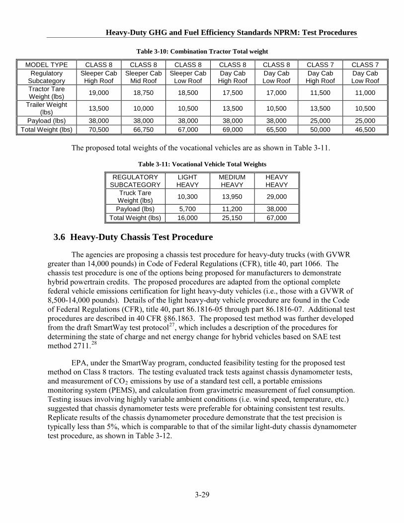
Heavy-Duty GHG and Fuel Efficiency Standards NPRM: Test Procedures
3-29
Table 3-10: Combination Tractor Total weight
MODEL TYPE CLASS 8 CLASS 8 CLASS 8 CLASS 8 CLASS 8 CLASS 7 CLASS 7 Regulatory
Subcategory Sleeper Cab High Roof
Sleeper Cab Mid Roof
Sleeper Cab Low Roof
Day Cab High Roof
Day Cab Low Roof
Day Cab High Roof
Day Cab Low Roof
Tractor Tare Weight (lbs) 19,000 18,750 18,500 17,500 17,000 11,500 11,000
Trailer Weight (lbs) 13,500 10,000 10,500 13,500 10,500 13,500 10,500
Payload (lbs) 38,000 38,000 38,000 38,000 38,000 25,000 25,000 Total Weight (lbs) 70,500 66,750 67,000 69,000 65,500 50,000 46,500
The proposed total weights of the vocational vehicles are as shown in Table 3-11.
Table 3-11: Vocational Vehicle Total Weights
REGULATORY SUBCATEGORY
LIGHT HEAVY
MEDIUM HEAVY
HEAVY HEAVY
Truck Tare Weight (lbs) 10,300 13,950 29,000
Payload (lbs) 5,700 11,200 38,000 Total Weight (lbs) 16,000 25,150 67,000
3.6 Heavy-Duty Chassis Test Procedure
The agencies are proposing a chassis test procedure for heavy-duty trucks (with GVWR greater than 14,000 pounds) in Code of Federal Regulations (CFR), title 40, part 1066. The chassis test procedure is one of the options being proposed for manufacturers to demonstrate hybrid powertrain credits. The proposed procedures are adapted from the optional complete federal vehicle emissions certification for light heavy-duty vehicles (i.e., those with a GVWR of 8,500-14,000 pounds). Details of the light heavy-duty vehicle procedure are found in the Code of Federal Regulations (CFR), title 40, part 86.1816-05 through part 86.1816-07. Additional test procedures are described in 40 CFR §86.1863. The proposed test method was further developed from the draft SmartWay test protocol27, which includes a description of the procedures for determining the state of charge and net energy change for hybrid vehicles based on SAE test method 2711.28
EPA, under the SmartWay program, conducted feasibility testing for the proposed test method on Class 8 tractors. The testing evaluated track tests against chassis dynamometer tests, and measurement of CO
2
Table 3-12
emissions by use of a standard test cell, a portable emissions monitoring system (PEMS), and calculation from gravimetric measurement of fuel consumption. Testing issues involving highly variable ambient conditions (i.e. wind speed, temperature, etc.) suggested that chassis dynamometer tests were preferable for obtaining consistent test results. Replicate results of the chassis dynamometer procedure demonstrate that the test precision is typically less than 5%, which is comparable to that of the similar light-duty chassis dynamometer test procedure, as shown in .

Draft Regulatory Impact Analysis
3-30
Table 3-12 Coefficients of Variation Reported for Chassis Dynamometer Tests Conducted Using the SmartWay Test Procedure.
METHOD OF EMISSIONS MEASUREMENT
TEST CELL PEMS GRAVIMETRIC
Truck number 29 555 598 29 555 598 29 555 598 UCT 12.7% 6.2% 1.6% 1.8% 0.8% 2.2% 3.9% 2.2% 2.0% LSC 2.0% 3.9% 1.4% 1.2% 0.3% 0.7% 2.1% 3.7% 0.7% HSC 1.3% 4.5% 1.0% 0.6% 0.5% 0.5% 1.7% 0.6% 1.2% Coefficient of variation is the standard deviation of the test replicates divided by the mean of the test replicates. UCT – Urban Creep and Transient duty cycle LSC -- Low Speed Cruise duty cycle HSC -- High Speed Cruise duty cycle
The number of heavy-duty chassis dynamometers in the United States is limited. EPA’s investigation found 11 chassis dynamometer sites in North America, including the following:
• Air Resources Board Heavy-Duty Emissions Testing Laboratory in Los Angeles, California
• California Truck Testing Services in Richmond, California • Colorado School of Mines, Colorado Institute for Fuels and Research in Golden,
Colorado • Environment Canada in Ottawa, Ontario, Canada • Southwest Research Institute in San Antonio, Texas • West Virginia University Transportable Heavy-Duty Vehicle Emissions Testing
Laboratory • National Renewable Energy Lab in Golden, Colorado • University of Houston in Houston, Texas • US EPA in Research Triangle Park (not in operation yet) • Argonne National Lab (up to 14,000 lb.) • National Vehicle Fuel and Emissions Lab in Ann Arbor, Michigan (up to 14,000 lb.)
3.7 Hybrid Powertrain Test Procedures
As discussed in Section II, the agencies see an opportunity to create incentives for use of hybrid powertrains in this proposal, to help drive the technology’s advancement. EPA and NHTSA are proposing two methods to demonstrate benefits of a hybrid powertrain – chassis and engine testing, and thereby generate credits through the use of such technology. The reduction in CO2 emissions and fuel consumption demonstrated would be available to use as credits in any vehicle or engine subcategory. That is, unlike ABT credits, credits generated by use of this technology would be available for use anywhere in the heavy-duty vehicle and engine sector. We are proposing the greater portability for these credits in order to create incentives to use this promising technology and thereby further its acceptance in the heavy-duty sector, with attendant GHG and fuel consumption reduction benefits.

Heavy-Duty GHG and Fuel Efficiency Standards NPRM: Test Procedures
3-31
The purpose of this testing provision is to allow for evaluation of greenhouse gas and fuel consumption reducing technologies that are available, but may lack broad market penetration beyond niche sectors. To effectively incentivize the introduction of this technology, as well as to accurately characterize its effectiveness, it is important to develop a standardized protocol as a basis for comparison. As described in the preamble for this rulemaking, the benefit of the hybridized version of the will be assessed based on a comparison to the conventional version. The basic methods considered for evaluation include full vehicle chassis testing of the hybrid system and powertrain evaluation in a configuration that does not include the full vehicle. The powertrain or “powerpack” testing may be undertaken in one of two ways. A powertrain test cell capable of accommodating the engine, complete hybrid system (including motor, power electronics, battery(ies), electronic control system, etc.), and the transmission may be used to evaluate post-transmission power pack systems. Engine dynamometer test cells may be used to assess the performance of the engine and hybrid power system with the control volume extending to just prior to the transmission. The distinction largely being the type of operation the engine – hybrid system can accommodate. When considering performance of any hybrid system, the durability of various emissions related system components will need to be included over the full regulatory useful life. While the industry and component manufacturers may be in the process of addressing battery technology and lifetime performance, any benefit associated with the hybrid system will be based on how this performance changes over the life of the hybrid system and vehicle.
Vehicle Chassis Dynamometer Testing
As a straightforward basis for addressing performance of hybrid systems for greenhouse gas emissions / fuel consumption reduction potential, the vehicle chassis dynamometer involves exercising the complete powertrain system within the vehicle for both conventional and hybrid systems. In this way, actual vehicle performance may be measured using prescribed duty cycles that have a real-world basis. The certification duty cycles considered for conventional heavy-duty vehicle certification may be applied to the hybrid vehicle system based on the proposed chassis testing protocols. The A to B testing would be conducted as described in Figure 3-3 Example of A to B Testing for Chassis or Powertrain Dynamometers below.
Figure 3-3 Example of A to B Testing for Chassis or Powertrain Dynamometers
Conventional Vehicle Hybrid Vehicle
Curb wt: 21k lbs
Payload: 1k lbs
Test wt: 22k lbs
Coastdown Wt: 22k lbs
GVWR: 33k lbs
Curb wt: 22k lbs
Payload: 1k lbs
Test wt: 23k lbs
Coastdown Wt: 23k lbs
GVWR: 33k lbs
A Test B Test

Draft Regulatory Impact Analysis
3-32
This approach is meant to account for the differences in vehicle weight expected for vehicles equipped with hybrid power systems. In so doing, the capability (e.g. payload, etc.) is not diminished for testing purposes. The expectation is that the benefit associated with the use of hybrid system may be characterized by the tractive operation duty cycles and / or the Power-Take Off duty cycle meant to better reflect the idle work and emissions saved through the use of a hybrid energy system. Chassis dynamometer testing for hybrid vehicles will be conducted using standard test protocols as described in SAE J1711 and 2711. To address the use of the power-take off and the GHG emissions related improvements associated with hybrid power systems, a separate duty as described in Table 3-14is provided. To address improvements for the purposes of credit generation, a weighted composite emission level will be used.
Powertrain / Powerpack Evaluation
To address hybrid power system performance for pre-vehicle testing configurations, this may be accomplished in a powertrain test cell or converted engine dynamometer test cell. There are various hardware-in-the-loop simulations being contemplated and implemented today, however the focus of this discussion will be on basic powertrain / powerpack evaluation. Any pre-vehicle testing provision that incorporates the benefits of hybrid power systems, would need to address several factors including durability of those components, kinetic energy recovery, design variety that could be captured using a chassis dynamometer test, and the drive cycle to appropriately characterize the vehicle activity. The testing methodologies for pre-vehicle hybrid evaluation currently consist of two equally viable strategies with different implications with respect to how emissions improvements are characterized. The first system to be discussed is the pre-transmission powerpack evaluation which incorporates all of the hybrid system components that exist prior to the transmission in the vehicle. The control volume is drawn so as to include the battery, battery support and control systems, power electronics, the engine, and motor generator and hybrid control module. The performance of this system is largely an engine based evaluation in which emission rates are determined on a brake-specific work basis. As such, the duty cycles being considered to assess this system performance are engine speed and torque command cycles. The emissions results associated with the system performance for GHG pollutants may be measured on brake-specific basis as an absolute test result. This differs from the approach used for post-transmission testing methods which may be conducted in a powertrain test cell or using a chassis dynamometer. As this rulemaking does not contemplate changes to criteria pollutant standards, the duty cycles and measurement methods may be similar to the criteria pollutants, however the emission results for GHG may be based on this full system consideration, which is not the case for criteria pollutants. Engine certification for criteria pollutant standards remain unchanged. It is expected that pre-transmission, parallel hybrids would be the most likely choice for engine-based hybrid certification.
For powertrain testing to determine hybrid benefit, the components mentioned for powerpack testing would be included for powertrain testing, as well as the transmission integrated with the hybrid power system. It is expected that testing could be conducted in a powertrain test cell which would differ from the traditional engine test cell in that it would need to accommodate the additional rotational inertia and speeds associated with inclusion of the vehicle / hybrid transmission with an electric, alternating current dynamometer. Additionally,

Heavy-Duty GHG and Fuel Efficiency Standards NPRM: Test Procedures
3-33
test cell control systems will need to address all relevant control factors including ways to integrate vehicle command data into the control strategy for the engine and hybrid transmission system. This could eventually include the need for vehicle and driver model inclusions into the control schema for test cell and test article.
Emissions testing for vehicles and hybrid powertrains will require A to B testing to determine the improvement factor as described in Preamble Section IV using the GEM result for the base vehicle model as the basis for assessing the CO2 performance improvement versus the appropriate vocational vehicle standard. Engine performance which includes the pre-transmission approach for hybrid certification will generate grams per brake-horsepower hour emissions result that should demonstrate improvement versus the base standard.
3.7.1 Chassis Dynamometer Evaluation
We are proposing that heavy-duty hybrid vehicles be certified using an A to B test method using a chassis dynamometer for testing vehicles. This concept allows the hybrid manufacturer to directly quantify the benefit associated with use of their hybrid system on an application specific basis. The concept would entail exercising the conventional vehicle, identified as “A”, tested over the defined cycles. The “B” vehicle would be the hybrid version of vehicle “A”. To be considered an appropriate “B” vehicle it must be the same exact vehicle model as the “A” vehicle. As an alternative, if no specific “A” vehicle exists for the hybrid vehicle that is the exact vehicle model, the most similar vehicle model must be used for certification. The most similar vehicle is defined as a vehicle with the same footprint, same payload, same intended service class, and the same coefficient of drag.
To determine the benefit associated with the hybrid system for greenhouse gas (GHG) performance, the weighted CO2
1. (CO
emissions results from the chassis test of each vehicle would define the benefit as described below:
2_A – CO2_B)/ (CO2_A2. Improvement Factor x Applicable Standard = ___ (g/ton mile benefit)
) = ______ (Improvement Factor)
Similarly, the benefit associated with the hybrid system for fuel consumption would be determined from the weighted fuel consumption results from the chassis tests of each vehicle as described below:
3. (Fuel C onsumptionA – Fuel C onsumptionB)/ ( Fuel ConsumptionA
4. Improvement Factor x F uel C onsumption S tandard = ___ (gallon/ton m ile benefit)
)= ______ (Improvement Factor)
3.7.1.1 Chassis Dynamometer Drive Cycles
The agencies are proposing two sets of duty cycles to evaluate the benefit depending on the vehicle application (such as delivery truck, bucket truck, or refuse truck). The key difference between these two sets of vehicles is that one does not operate a power take-off (PTO) unit while the other does.
Draft Regulatory Impact Analysis
3-34
A power take off (PTO) is a system on a vehicle that allows energy to be drawn from the vehicle’s drive system and used to power an attachment or a separate machine. Typically in a heavy-duty truck, a shaft runs from the transmission of the truck and operates a hydraulic pump. The operator of the truck can select to engage the PTO shaft in order for it to do work, or disengage the PTO shaft when the PTO is not required to do work. The pressure and flow from this hydraulic fluid can be used to do work in implements attached to the truck. Common examples of this are utility trucks that have a lift boom on them, refuse trucks that pick up and compact trash, and cement trucks that have a rotating barrel. In each case the auxiliary implement is typically powered by a PTO that uses energy from the truck’s primary drive engine.
In most PTO equipped trucks, it is necessary to run the primary drive engine at all times when the PTO might be needed. This is less efficient than an optimal system. Typical PTO systems require no more than 19 kW at any time, which is far below the optimal operation range of the primary drive engine of most trucks. Furthermore, in intermittent operations, the primary drive engine is kept running at all times in order to ensure that the PTO can operate instantaneously. This results in excess GHG emissions and fuel consumption due to idle time. Additionally, idling a truck engine for prolonged periods while operating auxiliary equipment like a PTO could cause the engine to cycle into a higher idle speed, wasting even more fuel. It would be possible to hybridize or change the operation of a conventional PTO equipped truck to lower the GHG emissions and fuel consumption in the real world. However, there is currently no method for an equipment manufacturer to demonstrate fuel consumption and GHG emissions reductions due to the application of advanced PTO technology. The proposed drive cycles do not allow for PTO operation to be included in the test protocol. We are proposing to add a new optional PTO test to the standard set of test cycles in order for manufacturers of advanced PTO systems to demonstrate in the laboratory environment fuel consumption and GHG reductions that would be realized from their systems in the real world. For this reason, the EPA contracted Southwest Research Institute (SwRI) to study PTO systems on heavy-duty trucks with a goal of determining an appropriate test cycle.
We worked with SwRI to review the heavy-duty truck market to determine what types of trucks used PTO’s and if the manufacturers thought that there was any possibility of commercial hybrid PTO applications. In some segments, manufacturers did not think a hybrid PTO was feasible. On the other hand, there are already utility and refuse trucks in existence that feature hybrid PTO units. We chose to study the behavior of conventional versions of these trucks in order to understand their typical operation.
We categorized the trucks based on the PTO opportunity. Trucks where limited PTO operation makes them infeasible due to low rates of return include dump trucks. Trucks where PTO operation is infeasible due to high power requirements include blower trucks, fire/emergency trucks, and concrete mixer trucks. Trucks where there is the possibility of PTO operation but there was no commercial interest include tow trucks, grapple trucks, and snowplow trucks.
We selected one utility truck that was in a rental fleet. Over the course of several weeks this truck was rented to two different customers and used in two different environments. The first time the truck was rented it was used in a rural setting outside of San Antonio, Texas. The following week the truck was used in a more urban setting in Fort Worth, Texas. Data was taken

Heavy-Duty GHG and Fuel Efficiency Standards NPRM: Test Procedures
3-35
from the truck as follows: - Engine Speed, Engine Fuel Rate, Vehicle Speed, PTO Pressure, and PTO Flow Rate.
From this data we were able to determine how often the truck’s engine was running, how often the PTO was engaged, and how often the boom of the utility truck was being manipulated by the user. The field data showed that when the truck was operated in the rural setting it had a much lower rate of utilization that when it was operated in the urban setting. Table 3-13 shows a breakdown of the operation of the truck in each setting.
Table 3-13 Utility Truck PTO Operation
RURAL SETTING URBAN SETTING % Time PTO at “Idle” 90% 50% % Time PTO working 10% 50%
In order to better understand the field operation of refuse trucks, EPA commissioned SwRI to study the operation of a refuse hauling truck. SwRI worked with Waste Management in Conroe Texas to instrument a typical PTO equipped neighborhood pickup refuse hauler. The truck that we instrumented was equipped with a side-load-arm (SLA). Southwest’s research revealed that approximately 20 percent of the trucks in the industry include an SLA, and the percentage of trucks with an SLA is increasing. Also, a truck with an SLA is able to service more homes per day than a standard truck, so as more SLA equipped trucks are added to the fleet, the total number of trucks will decrease.
The refuse truck was driven on its various routes over the course of a week and the data recorded. Though the truck operated on different streets and areas within the city of Conroe each day, the operation characteristics of the truck were uniform day-to-day.
Once the data was collected, definitions of power take-off (PTO) operations were identified as (1) pump “on” and idle (utility truck), and (2) compactor only, loader only, both compactor and loader, and idle (refuse truck). Steady-state pressure modes were identified by a statistical disjoint cluster analysis. Statistical frequency analyses of the in-field data were used to determine the relative proportion of time allocated to each steady-state mode. The loader and compactor pressure data from the refuse truck demonstrated cyclical behavior, therefore, a discrete Fourier transform using the fast Fourier transform (FFT) algorithm was performed on the loader and compactor data independently. The results of the FFT were used to determine the frequency of the modes in the test cycle. Information collected on population usage was used to weight different portions of the composite duty cycle (utility and refuse truck cycles) to reflect actual field PTO operations.
Based upon the results of the data collection, we decided that a representative duty cycle for PTO operation would not begin until the engine was fully warmed up. In all cases the trucks were warmed up before driving, then driven some distance to a location where the PTO was engaged. Thus, the traction engine was always fully warm before PTO operation commenced.
Based upon the data collection we believe that a representative PTO cycle should test a PTO that is at operating temperature. In the case of the utility truck, most of the operation is in an urban environment and about one-half of the operation time is loaded. Thus, the PTO would

Draft Regulatory Impact Analysis
3-36
only operate in a “cold” state for less than 2% of a typical day. The refuse truck showed similar operation, the PTO was run continuously throughout the eight hour work day resulting in cold operation of the PTO for less than 2% of the typical day.
EPA and NHTSA are proposing that truck manufacturers be able to test their PTO system and compare it to a baseline system to generate GHG emissions and fuel consumption credits. The manufacturer will need to test their system in an emissions cell capable of measuring GHG emissions. The PTO would be exercised by an auxiliary test bench and commanded to follow a prescribed cycle. The cycle will be determined by the type of PTO system that is under consideration. At this time, PTO cycles have been developed for utility trucks and refuse hauling trucks.
The agencies are proposing a composite PTO cycle to allow PTO manufacturers to earn credits for GHG emissions. The cycle we are proposing has been weighted based on the utility truck and refuse truck data in the SwRI report. It was determined that utility truck usage was approximately 20 percent rural and 80 percent urban. Furthermore, based on the field data obtained from the test trucks, the utility trucks are expected to use the PTO when performing boom operations 10 percent of the time in rural settings and 50 percent of the time in urban settings. The data from the refuse truck in the SwRI report was used to complete the refuse portion of the cycle. Because the refuse truck used in the data collection had two hydraulic circuits, one for the load arm and one for the compactor, there are two pressure traces, one for each circuit. Thus, the PTO test cycle described in Table 3-14 reflects this.

Heavy-Duty GHG and Fuel Efficiency Standards NPRM: Test Procedures
3-37
Table 3-14: Proposed PTO Cycle
Cycle Simulation
Mode Time Normalized Pressure, Circuit 1 (%)
Normalized Pressure, Circuit 2 (%)
Utility 0 0 0.0 0.0 Utility 1 33 80.5 0.0 Utility 2 40 0.0 0.0 Utility 3 145 83.5 0.0 Utility 4 289 0.0 0.0 Refuse 5 361 0.0 13.0 Refuse 6 363 0.0 38.0 Refuse 7 373 0.0 53.0 Refuse 8 384 0.0 73.0 Refuse 9 388 0.0 0.0 Refuse 10 401 0.0 13.0 Refuse 11 403 0.0 38.0 Refuse 12 413 0.0 53.0 Refuse 13 424 0.0 73.0 Refuse 14 442 11.2 0.0 Refuse 15 468 29.3 0.0 Refuse 16 473 0.0 0.0 Refuse 17 486 11.2 0.0 Refuse 18 512 29.3 0.0 Refuse 19 517 0.0 0.0 Refuse 20 530 12.8 11.1 Refuse 21 532 12.8 38.2 Refuse 22 541 12.8 53.4 Refuse 23 550 12.8 73.5 Refuse 24 553 0.0 0.0 Refuse 25 566 12.8 11.1 Refuse 26 568 12.8 38.2 Refuse 27 577 12.8 53.4 Refuse 28 586 12.8 73.5 Refuse 29 589 0.0 0.0 Refuse 30 600 0.0 0.0
The protocol for testing the PTO system will be similar to chassis testing. The vehicle will be positioned such that the exhaust system can be attached to exhaust emission analyzers. This can be done using, but does not necessarily require, a chassis dynamometer. The PTO system will be disconnected from the truck’s work absorbing apparatus and connected to a bench

Draft Regulatory Impact Analysis
3-38
that will provide energy absorption to the PTO system. For trucks with one hydraulic circuit in the PTO system, they will be hooked up to the utility/compactor side of the PTO bench. Trucks with two hydraulic circuits will be hooked up to both circuits on the PTO bench. A schematic of this bench can be seen in Appendix I. The vehicle will be pre-conditioned at ambient conditions and then the engine will be run until it is at operating temperature. The PTO will then be exercised until the working fluid and or driving mechanism of the PTO is up to operating temperature. The fully warmed up operating temperature may be defined by the manufacturer or may be assumed to be 150°C. The test will then commence. We believe that a “hot-start” test is appropriate because our data analysis found that trucks equipped with PTO’s are nearly always warmed up before the PTO is used, and that cold PTO operation makes up less than 2% of a PTO’s typical daily usage.
The PTO would be manipulated by the operator to the prescribed duty cycle. GHG emissions and fuel consumption will be measured as well as criteria pollutants. GHG emissions and fuel consumption would be reported to determine credits; criteria pollutants will simply be reported.
In order to gain credits the manufacturer would have to demonstrate how a truck with a conventional PTO system would perform over the same duty cycle. Both sets of data will need to be measured and reported to EPA and NHTSA in order to claim GHG emission and fuel consumption credits.
The first set of proposed duty cycles would apply to the hybrid powertrains used to improve the motive performance of the vehicle (such as pickup and delivery trucks). The typical operation of these vehicles is very similar to the proposed drive cycles. Therefore, the agencies are proposing to use the vocational vehicle weightings for these vehicles, as shown in Table 3-12. We are using the proposed regulatory vocational vehicle classifications for the ABT vocational vehicle classification. Hybrid vehicles used in applications such as utility and refuse trucks tend to have additional benefit associated with use of stored energy, which avoids main engine operation and related CO2 emissions and fuel consumption. To appropriately address these alternative sources for benefits, exercising the conventional and hybrid vehicles using their PTO would help to quantify the benefit to GHG emissions and fuel consumption reductions. The duty cycle proposed to quantify the hybrid CO2
Table 3-15
and fuel consumption impact over this broader set of operation would be the three primary cycles plus a PTO duty cycle. The proposed weighting for the cycle is based on data gathered during the SwRI study. Based on fleet owner information, the agencies estimate that the utility trucks are used 20 percent of the time in rural operations and 80 percent of the time in urban operations. The SwRI study found that utility trucks spent 5.5 percent of the time operating the PTO in rural settings and 34.4 percent of the time on in urban settings. This produces an overall percent PTO on time for utility trucks of 28.6 percent. The study found that the refuse trucks have the PTO on 26.7 percent of the time. The agencies weighted each truck type’s percent on time based on 40 percent refuse trucks and 60 percent utility trucks to establish an overall 28 percent on-time. Therefore, the agencies are proposing that the PTO cycle be weighted at 28 percent and weight the other three cycles for the remaining 72 percent. The proposed weightings for the hybrids with and without PTO are included in .

Heavy-Duty GHG and Fuel Efficiency Standards NPRM: Test Procedures
3-39
Table 3-15: Proposed Drive Cycle Weightings for Hybrid Vehicles
Transient 55 mph 65 mph PTO Vocational Vehicles without PTO 42% 21% 37% 0% Vocational Vehicles with PTO 30% 15% 27% 28%
3.7.2 Engine Dynamometer Evaluation
The engine test procedure we are proposing for hybrid evaluation involves exercising the conventional engine and hybrid-engine system based on an engine testing strategy. The basis for the system control volume, which serves to determine the valid test article, will need to be the most accurate representation of real world functionality. An engine test methodology would be considered valid to the extent the test is performed on a test article that does not mischaracterize criteria pollutant performance or actual system performance. Energy inputs should not be based on simulation data which is not an accurate reflection of actual real world operation. It is clearly important to be sure credits are generated based on known physical systems. This includes testing using recovered vehicle kinetic energy. Additionally, the duty cycle over which this engine-hybrid system will be exercised must reflect the use of the application, while not promoting a proliferation of duty cycles which prevent a standardized basis for comparing hybrid system performance. The agencies are proposing the use of the Heavy-Duty Engine FTP cycle for evaluation of hybrid vehicles, which is the same test cycle proposed for engines used in vocational vehicles. It is important that introduction of clean technology be incentivized without compromising the program intent of real world improvements in GHG and fuel consumption performance.
Pre-transmission power-pack testing would involve the power system components included in the engine test cell up to the transmission (pre-gearbox) as the valid test article. The engine power would serve as the basis for assessing brake specific emissions performance for criteria pollutants as the agencies are not proposing changes to the criteria pollutant standards. For GHG pollutant performance, the entire power system pre-gearbox can serve as the basis for the brake-specific emissions performance as seen in
Pre-Transmission Power-Pack Testing
Figure 3-4 Pre-Transmission Parallel Hybrid Power Pack Test Configuration. Testing using this method, as described previously, could utilize existing engine certification duty cycles. The applicability to the broader set of applications could be based largely on the approach taken with today’s engine certification. Changes to how the engine certification would be conducted to address energy capture and idle operation will need to be evaluated as a complete protocol is developed. In conducting hybrid testing it is important for the RESS to have a state of charge at the end of the certification test to have a net change in the state of charge of less than 1%. It has been suggested to the agencies that energy capture for pre-transmission, parallel hybrid, power-pack testing could be based on one of the following three approaches: allow capture up to capability of system, place upper limit on energy captured over cycle based on available brake energy in real world cycles, or calculate second-by-second available regeneration torque based on FTP29.

Draft Regulatory Impact Analysis
3-40
Figure 3-4 Pre-Transmission Parallel Hybrid Power Pack Test Configuration
Source: Cummins Incorporated’s White Paper: Regulation of emissions from commercial hybrid vehicles, August 9, 2010
Post-transmission power-pack testing would involve the power system components included in the engine test cell up to and including the transmission (potentially still pre-gearbox) as the valid test article. The inclusion of the transmission in the hybrid system for certification potentially introduced a new entity to the certification and a new aspect to of test article control. With the additional components, the traditional FTP is not viable, in its current form for exercising a more complete powertrain. A vehicle-like duty cycle which provides the appropriate speeds and torques to more appropriately match field operation would be needed. The test article anticipated for this configuration, would more closely match complete hardware in the loop evaluation methods contemplated in other testing regimes. The ability to obtain actual performance results versus simulations of actual results in a test environment largely center on evaluating components with native intelligence rather than simulating their control system.
Post-Transmission Power-Pack Testing
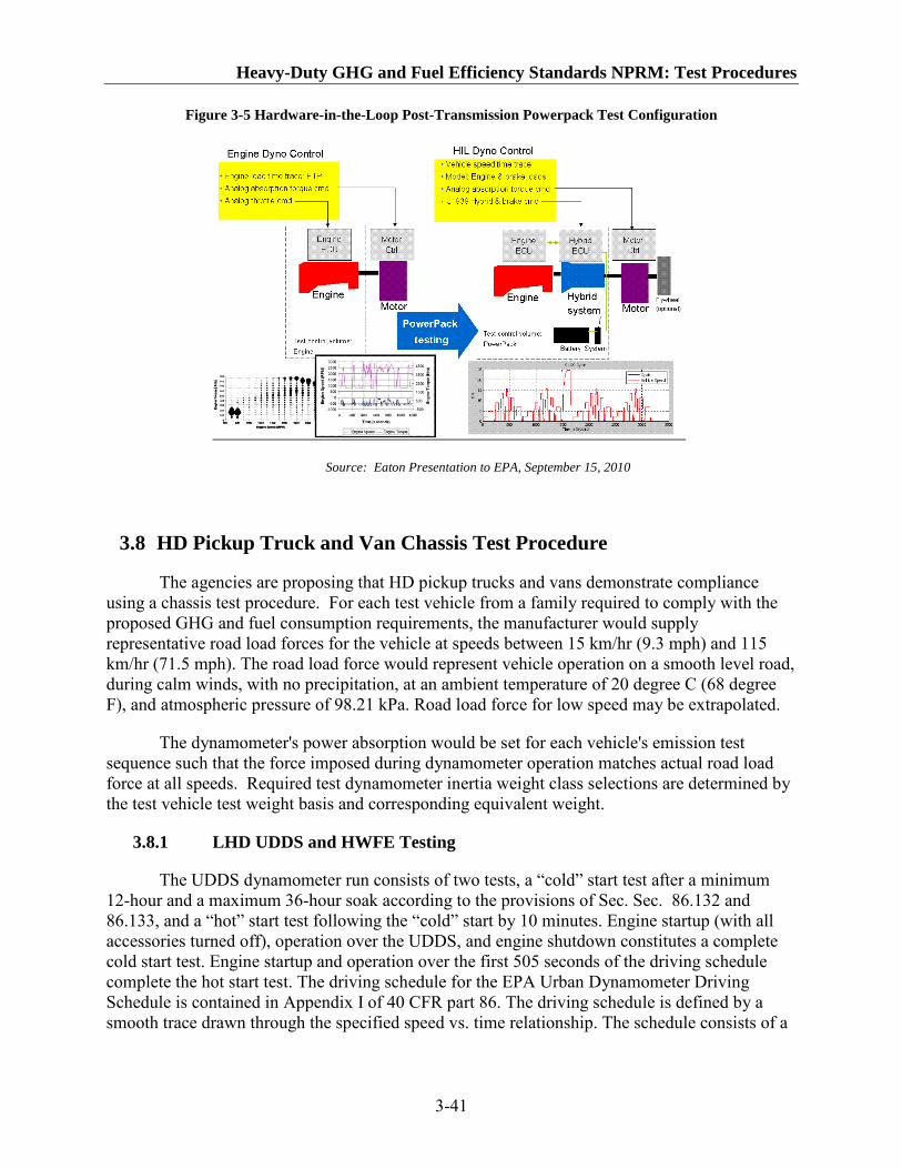
Heavy-Duty GHG and Fuel Efficiency Standards NPRM: Test Procedures
3-41
Figure 3-5 Hardware-in-the-Loop Post-Transmission Powerpack Test Configuration
Source: Eaton Presentation to EPA, September 15, 2010
3.8 HD Pickup Truck and Van Chassis Test Procedure
The agencies are proposing that HD pickup trucks and vans demonstrate compliance using a chassis test procedure. For each test vehicle from a family required to comply with the proposed GHG and fuel consumption requirements, the manufacturer would supply representative road load forces for the vehicle at speeds between 15 km/hr (9.3 mph) and 115 km/hr (71.5 mph). The road load force would represent vehicle operation on a smooth level road, during calm winds, with no precipitation, at an ambient temperature of 20 degree C (68 degree F), and atmospheric pressure of 98.21 kPa. Road load force for low speed may be extrapolated.
The dynamometer's power absorption would be set for each vehicle's emission test sequence such that the force imposed during dynamometer operation matches actual road load force at all speeds. Required test dynamometer inertia weight class selections are determined by the test vehicle test weight basis and corresponding equivalent weight.
3.8.1 LHD UDDS and HWFE Testing
The UDDS dynamometer run consists of two tests, a “cold” start test after a minimum 12-hour and a maximum 36-hour soak according to the provisions of Sec. Sec. 86.132 and 86.133, and a “hot” start test following the “cold” start by 10 minutes. Engine startup (with all accessories turned off), operation over the UDDS, and engine shutdown constitutes a complete cold start test. Engine startup and operation over the first 505 seconds of the driving schedule complete the hot start test. The driving schedule for the EPA Urban Dynamometer Driving Schedule is contained in Appendix I of 40 CFR part 86. The driving schedule is defined by a smooth trace drawn through the specified speed vs. time relationship. The schedule consists of a

Draft Regulatory Impact Analysis
3-42
distinct non-repetitive series of idle, acceleration, cruise, and deceleration modes of various time sequences and rates.
The Highway Fuel Economy Dynamometer Procedure (HFET) consists of preconditioning highway driving sequence and a measured highway driving sequence. The HFET is designated to simulate non-metropolitan driving with an average speed of 48.6 mph and a maximum speed of 60 mph. The cycle is 10.2 miles long with 0.2 stop per mile and consists of warmed-up vehicle operation on a chassis dynamometer through a specified driving cycle. The Highway Fuel Economy Driving Schedule is set forth in Appendix I of 40 CFR Part 600. The driving schedule is defined by a smooth trace drawn through the specified speed versus time relationships.
Practice runs over the prescribed driving schedules may be performed at test point, provided an emission sample is not taken, for the purpose of finding the appropriate throttle action to maintain the proper speed-time relationship, or to permit sampling system adjustment. Both smoothing of speed variations and excessive accelerator pedal perturbations are to be avoided. The driver should attempt to follow the target schedule as closely as possible. The speed tolerance at any given time on the dynamometer driving schedules specified in Appendix I of parts 40 and 600 is defined by upper and lower limits. The upper limit is 2 mph higher than the highest point on trace within 1 second of the given time. The lower limit is 2 mph lower than the lowest point on the trace within 1 second of the given time. Speed variations greater than the tolerances (such as may occur during gear changes) are acceptable provided they occur for less than 2 seconds on any occasion. Speeds lower than those prescribed are acceptable provided the vehicle is operated at maximum available power during such occurrences.
3.8.2 LHD UDDS and HWFE Hybrid Testing
Since LHD chassis certified vehicles share test schedules and test equipment with much of Light-Duty Vehicle testing, EPA believes it is appropriate to reference SAE J1711 “Recommended Practice for Measuring the Exhaust Emissions and Fuel Economy of Hybrid-Electric Vehicles, Including Plug-in Hybrid Vehicles” instead of SAEJ2711 “Recommended Practice for Measuring Fuel Economy and Emissions of Hybrid-Electric and Conventional Heavy-Duty Vehicles”.
3.8.2.1 Charge Depleting Operation – FTP or “City” Test and HFET or “Highway” Test
The EPA would like comment on incorporating by reference SAE J1711 chapters 3 and 4, as published June 2010, testing procedures for Light-Heavy-Duty chassis certified vehicles with the following exceptions and clarifications:
Test cycles will continue until the end of the phase in which charge sustain operation is confirmed. Charge sustain operation is confirmed when one or more phases or cycles satisfy the Net Energy Change requirements below. Optionally, a manufacturer may terminate charge deplete testing before charge sustain operation is confirmed provided that the Rechargeable Energy Storage System (RESS) has a higher State of Charge (SOC) at charge deplete testing
Heavy-Duty GHG and Fuel Efficiency Standards NPRM: Test Procedures
3-43
termination than in charge sustain operation. In the case of Plug In Hybrid Electric Vehicles (PHEV) with an all electric range, engine start time will be recorded but the test does not necessarily terminate with engine start. PHEVs with all electric operation follow the same test termination criteria as blended mode PHEVs. Testing can only be terminated at the end of a test cycle. The Administrator may approve alternate end of test criteria.
For the purposes of charge depleting CO2
End of test recharging procedure is intended to return the RESS to a full charge equivalent to pre test conditions. The recharge AC watt hours must be recorded throughout the charge time and soak time. Vehicle soak conditions must not be violated. The AC watt hours must include the charger efficiency. The measured AC watt hours are intended to reflect all applicable electricity consumption including charger losses, battery and vehicle conditioning during the recharge and soak, and the electricity consumption during the drive cycles.
and fuel efficiency testing, manufacturers may elect to report one measurement per phase (one bag per UDDS). Exhaust emissions need not be reported or measured in phases the engine does not operate.
Net Energy Change Tolerance (NEC), is to be applied to the RESS to confirm charge sustaining operation. The EPA intends to adopt the 1% of fuel energy NEC state of charge criteria as expressed in SAE J1711. The Administrator may approve alternate NEC tolerances and state of charge correction factors.
3.8.2.2 Hybrid Charge Sustaining Operation – FTP or “City” Test and HFET or “Highway” Test
The EPA proposes to incorporate by reference SAE J1711 chapters 3 and 4 for definitions and test procedures, respectively, where appropriate, with the following exceptions and clarifications.
The EPA proposes to adopt the 1% of fuel energy NEC state of charge criteria as expressed in SAEJ1711. The Administrator may approve alternate NEC tolerances and state of charge correction factors.
Preconditioning special procedures are optional for traditional “warm” test cycles that are now required to test starting at full RESS charge due to charge depleting range testing. If the vehicle is equipped with a charge sustain switch, the preconditioning cycle may be conducted per 600.111 provided that the RESS is not charged. Exhaust emissions are not taken in preconditioning drives. Alternate vehicle warm up strategies may be approved by the Administrator.
State of Charge tolerance correction factors may be approved by the Administrator. RESS state of charge tolerances beyond the 1% of fuel energy may be approved by the Administrator.
The EPA is seeking comment on modifying the minimum and maximum allowable test vehicle accumulated mileage for both EVs and PHEVs. Due to the nature of PHEV and EV operation, testing may require many more vehicle miles than conventional vehicles. Furthermore, EVs and PHEVs either do not have engines or may use the engine for only a fraction of the miles driven.

Draft Regulatory Impact Analysis
3-44
Electric Vehicles and PHEVs are to be recharged using the supplied manufacturer method provided that the methods are available to consumers. This method could include the electricity service requirements such as service amperage, voltage, and phase. Manufacturers may employ the use of voltage regulators in order to reduce test to test variability with prior Administrator approval.

Heavy-Duty GHG and Fuel Efficiency Standards NPRM: Test Procedures
3-45
1 Coordinating Research Council, Inc. Phase 1 of the Advanced Collaborative Emissions Study. June 2009.
References
2 Fiest, M., C. Sharp, R. Mason, J. Buckingham. Determination of PEMS Measurement Allowances for Gaseous Emissions Regulated Under the Heavy-Duty Diesel Engine In-Use Testing Program.2007. Table 122 and 123. 3 § 86.004-28 4 U.S. EPA. Truck and Trailer Roof Height Match Analysis Memorandum from Amy Kopin to the Docket, August 9, 2010. Docket Identification Number EPA-HQ-OAR-2010-0162-0045. 5 SAE Recommended Practice 1263, Road Load Measurement and Dynamometer Simulation Using Coastdown Techniques, January 2009 6 SAE Recommended Practice J2263. Road Load Measurement Using Onboard Anemometry and Coastdown Techniques. December 2008. 7 “Heavy-Duty Coastdown Test Procedure Development,” Docket Number EPA-HQ-OAR-2010-0162-0144. 8 "Lecture Notes in Applied and Computational Mechanics, The Aerodynamics of Heavy Vehicles II: Trucks, Buses, and Trains; DOI: 10.1007/978-3-540-85070-0_33; “Applicability of Commercial CFD tools for assessment of heavy vehicle aerodynamic characteristics” as created by the University of Chicago as Operator of Argonne National Laboratory (“Argonne”) under contract No. W-31-109-ENG-38 with the U.S. Department of Energy." 9 For more information, see CFR Title 40, Part 86.129-00 (e)(1). 10 2010 NAS Report. Finding 2-4 on page 39. 11 SAE International, 2006, Rolling Resistance measurement Procedure for Passenger Car, Light Truck, and Highway Truck and Bus Tires, SAE J1269, 2006-09 12 ISO, 2009, Passenger Car, Truck, and Bus Tyres – Methods of Measuring Rolling Resistance – Single Point Test and Correlation of Measurement Results: ISO 28580:2009(E), First Edition, 2009-07-01 13 NHTSA, 2009. “NHTSA Tire Fuel Efficiency Consumer Information Program Development: Phase 1 – Evaluation of Laboratory Test Protocols.” DOT HS 811 119. June. (www.regulations.gov, Docket ID: NHTSA-2008-0121-0019). 14 SAE International, 1999, Stepwise Coastdown Methodology for Measuring Tire Rolling Resistance,. SAE J2452, 1999-06 15 ISO, 2005, Passenger Car, Truck, Bus, and Motorcycle Tyres – Methods of Measuring Rolling Resistance, ISO 18164:2005(E) 16 Based on MOVES analysis. 17 University of California Riverside. Analysis of Heavy Duty Diesel Truck Activity and Emissions Data. 2006. 18 Gaines, L. “Estimation of Fuel Use by Idling Commercial Trucks”, Paper 06-2567. 2006. 19 Franzese, O., H. Knee, L. Slezak. Effect of Tires on Class-8 Heavy Truck Fuel Efficiency. July 2009. Last viewed on May 1, 2010 at http://info.ornl.gov/sites/publications/files/Pub20686.pdf 20 U.S. Department of Energy. “Transportation Energy Data Book. Edition 28 – 2009. Table 5.11. Last viewed on Mary 1, 2010 at http://cta.ornl.gov/data/tedb28/Edition28_Chapter05.pdf 21 Environmental Defense Fund. “Greenhouse Gas Management for Medium-Duty Truck Fleets.” Viewed at http://edf.org/documents/10860_fleets-med-ghg-management.pdf. Page 6. 22 ICF International. Investigation of Costs for Strategies to Reduce Greenhouse Gas Emissions for Heavy-Duty On-Road Vehicles. July 2010. Pages 4-16. Docket Identification Number EPA-HQ-OAR-2010-0162-0044.

Draft Regulatory Impact Analysis
3-46
23 M.J. Bradley & Associates. Setting the Stage for Regulation of Heavy-Duty Vehicle Fuel Economy and GHG Emissions: Issues and Opportunities. February 2009. Page 35. Analysis based on 1992 Truck Inventory and Use Survey data, where the survey data allowed developing the distribution of loads instead of merely the average loads. 24 The U.S. Federal Highway Administration. Development of Truck Payload Equivalent Factor. Table 11. Last viewed on March 9, 2010 at http://ops.fhwa.dot.gov/freight/freight_analysis/faf/faf2_reports/reports9/s510_11_12_tables.htm 25 Excerpted from The U.S. Federal Highway Administration. Development of Truck Payload Equivalent Factor. Table 11. Last viewed on March 9, 2010 at http://ops.fhwa.dot.gov/freight/freight_analysis/faf/faf2_reports/reports9/s510_11_12_tables.htm 26 The U.S. Federal Highway Administration. Development of Truck Payload Equivalent Factor. Table 11. Last viewed on March 9, 2010 at http://ops.fhwa.dot.gov/freight/freight_analysis/faf/faf2_reports/reports9/s510_11_12_tables.htm 27 U.S. Environmental Protection Agency, SmartWay Fuel Efficiency Test Protocol for Medium and Heavy Duty Vehicles – Working Draft, EPA420-P-07-003, November 2007, http://www.epa.gov/smartway/transport/documents/tech/420p07003.pdf, site accessed September 16, 2009. 28 SAE Recommended Practice for Measuring Fuel Economy and Emissions of Hybrid Electric and Heavy-Duty Vehicles, September 1, 2002 29 Cummins Incorporated, Regulation of Emissions from Commercial Hybrid Vehicles, August 2010

Heavy-Duty GHG and Fuel Efficiency Standards NPRM: Vehicle Simulation Model
4-1
Chapter 4: Vehicle Simulation Model 4.1 Purpose and Scope
4.1.1 Methods to Assess a Truck’s Greenhouse Gas Emissions
An important aspect of a regulatory program is to determine the environmental benefits of heavy-duty truck technologies through testing and analysis. There are several methods available today to assess greenhouse gas emissions from trucks. Truck fleets today often use SAE J1321 test procedures to evaluate criteria pollutant emissions changes based on paired truck testing.1 Light-duty trucks are assessed using chassis dynamometer test procedures.2 Heavy-duty engines are evaluated with engine dynamometer test procedures.3
4.1.2 Proposal to Use Simulation Model to Certify Vocational Trucks and Combination Tractors
Most large truck manufacturers employ various computer simulation methods to estimate truck efficiency. Each method has advantages and disadvantages. This section will focus on the use of truck simulation modeling for assessing tailpipe GHG emissions and fuel consumption.
The agencies are proposing to use a simulation model as the primary tool to certify vocational and combination tractor heavy-duty vehicles (Class 2b through Class 8 heavy-duty, vehicles that are not heavy-duty pickups or vans). The advantages of modeling for these vehicles include:
• The simulation tool can model a wide range of vehicle types.
• The vehicle components can be easily changed to match the features of a given vehicle.
• The entire configuration of the vehicle can also be changed, so the same program can model a Class 4 pickup and delivery truck and a Class 7 or 8 combination truck with appropriate input parameter changes. This allows the agencies to use the same program to develop and certify all of the heavy-duty vehicles.
• The modeling tool also accommodates different drive cycles.
• It can significantly reduce truck manufacturer’s burden to conduct heavy-duty chassis dynamometer tests.
4.1.3 Chapter Overview
The scope of this chapter will discuss truck simulation models and their feasibility, the truck simulation tool, and application of models to develop certification options.

Draft Regulatory Impact Analysis
4-2
4.2 Model Code Description
4.2.1 Engineering Foundations of Model
A number of commercially available heavy-duty vehicle simulation tools are based on MATLAB/Simulink-based programs that can model a wide variety of vehicles, from medium-duty to Class 8 trucks.4,5 Generally, each vehicle component is depicted by a generic Simulink model that can be modified using an initialization file.6
EPA has developed a forward-looking MATLAB/Simulink-based model termed Greenhouse gas Emissions Model (GEM) for Class 2b-8 vehicle compliance. GEM uses the same physical principles as many other existing vehicle simulation models to derive governing equations which describe driveline components, engine, and vehicle. These equations are then integrated in time to calculate transient speed and torque.
The user can utilize pre-determined initialization files for a given component, or modify them to reflect their particular situation. The following section describes the system required to model a heavy-duty non-hybrid truck. Once the vehicle has been specified, the user selects a drive cycle (which they can also modify) and runs the program.
4.2.2 Vehicle Model Architecture
Table 4-1 outlines the Class 2b-8 vehicle compliance model architecture, which is comprised of six systems: Ambient, Driver, Electric, Engine, Transmission, and Vehicle. With the exception of “Ambient” and “Driver,” each system consists of two to four component models. The function of each system and their respective component models, wherever applicable, is discussed in this section.
Table 4-1: Vehicle Model Architecture
System Component Models Ambient none Driver none Electric Starter; Electrical Energy System; Alternator; Accessory (electrical) Engine Cylinder; Accessory (mechanical) Transmission Clutch; Gearbox Vehicle Chassis; Final Drive
Ambient – This system defines ambient conditions such as pressure, temperature, and road gradient, where vehicle operations are simulated.
Driver – GEM is a forward-looking driving model. Rather than constantly matching the exact drive cycle, the driver model considers the current speed and the desired future speed to try to predict the necessary power required to close the gap and follow the driving trace. If the driver misses the target, a different power request is sent to the engine and/or brakes are applied. This search for the proper vehicle speed occurs at every simulation time step. The feedback loop uses a PID controller.
The “Electric” system consists of four components: Starter, Electrical Energy System, Alternator, and Electrical Accessory

Heavy-Duty GHG and Fuel Efficiency Standards NPRM: Vehicle Simulation Model
4-3
Starter – This models the starter for the engine, which is identical for most vehicles.
Electrical Energy System – GEM simulates a standard 12 or 24 volt lead-acid battery, which provides currents to the starter and electrical systems for engine starting, lighting, and vehicle controls. This module estimates State-of-Charge (SOC), internal ohmic resistance and open circuit voltage, voltage and current of electrical energy storage system.
Alternator – This models the alternator that generates electricity for the battery and electrical system. The model calculates voltage and current of the AC alternator based on alternator performance maps and charge control strategy.
Electrical Accessory – All vehicles have a number of electrical loads, some of which are necessary to operate the vehicle. The engine control unit (ECU), fuel injectors and fuel pump for instance are electrical loads that are constantly on the battery, and these are already taken into account in the fuel map.
The “Engine” system consists of two components: Cylinder and Mechanical Accessory
Cylinder – The cylinder model is based on a fuel map and torque curves at wide open throttle (full load) and closed throttle (no load). The engine fuel map features three sets of data: engine speed, torque, and fueling rate at pre-specified engine speed and torque intervals. It is not a physics-based model and does not attempt to model in-cylinder combustion process. The engine torque and speed are used to select a fuel rate based on the fuel map. This map is adjusted automatically by taking into account three different driving types: acceleration, braking, and coasting. The fuel map, torque curves, and the different driving types are pre-programmed into GEM for several different default engines.
Mechanical Accessory – Most vehicles run a number of accessories that are driven via mechanical power from the engine. Some of these accessories are necessary for the vehicle to run, like the coolant pump, while others are only used occasionally and at the operator’s discretion such as the air conditioning compressor. Some heavy-duty vehicles also use Power Take Off (PTO) to operate auxiliary equipment, like booms, and these would also be modeled as a mechanical accessory.
The manual “Transmission” system consists of two components: a Clutch and a Gearbox
Clutch – This component model simulates the clutch for a manual transmission.
Gearbox – A simple gearbox model is used for a manual transmission, and the number of gears and gear ratios is predefined in GEM. This component model consists of a map using gearbox speed and torque as inputs to model the efficiency of each gear.
The “Vehicle” system consists of two components: Chassis and Final Drive
Chassis – This portion models the shell of the vehicle including the tires. The drag coefficient, mass of the vehicle, frontal area and other parameters are housed in this component. For tire simulation, the user specifies the configuration of each axle on the vehicle, including the tire diameter and the rolling resistance.

Draft Regulatory Impact Analysis
4-4
Final Drive – The gear ratio for the differential can be specified directly by the user. The efficiency is defined by a map based on the transmission output speed and torque.
4.2.3 Capability, Features, and Computer Resources
The EPA/NHTSA vehicle compliance tool is a flexible simulation platform that can model a wide variety of vehicles from Class 2b to Class 8 trucks. The key to this flexibility is the MATLAB component files that can be modified or adjusted to accommodate vehicle-specific information. Parameters such as vehicle weight, fuel map settings, and tire radius, for instance, can all be changed in this fashion. However, since the proposed rule specifies applicable drive cycles (the Transient mode, as defined by ARB in the HHDDT cycle, a constant speed cycle at 65 mph and a 55 mph constant speed mode), manufacturers cannot select alternative drive cycles (although the model is capable of incorporating other drive cycles should the agencies decide after considering public comment that additional or different drive cycles are necessary). Similarly, manufacturers cannot alter any default settings which are established by the agencies.
After running the simulation, GEM tracks information about each component and about the system as a whole. Information like CO2
The system requirements for the MATLAB version of GEM include a minimum RAM of 1 GB, MATLAB, Simulink and Stateflow (version 2009b or later), and approximately 250 MB of disk storage.
emissions, fuel consumption, and fidelity to the drive cycle are immediately available on the results screen. The output from each run can be saved as a comma-separated values (CSV) file or an Excel file.
7,8,9
4.3 Feasibility of Using a Model to Simulate Testing
The simulation takes between 10 and 20 seconds per drive cycle, depending on the cycle duration. No separate license is required to run the program other than for MATLAB, Simulink, and Stateflow. Although the source code is available to users, all of the component initialization files, control strategies and the underlying MATLAB/Simulink/Stateflow-based models should remain fixed and should not be manipulated by the users when assessing their compliance. For these reasons, a stand-alone executable model independent of MATLAB/Simulink/Stateflow licenses has been created. Only the executable can be used when producing official truck certification results. The agencies are proposing that the manufacturers submit both the input parameters and the modeling results.
4.3.1 Procedure for Model Validation
The agencies have assessed the predictive utility of the GEM model by comparing its prediction with actual test data. The agencies plan to continue this effort between proposal and final rule, and also plan to continue the supplemental validation effort where GEM predictions are compared with those of a widely-used commercial model. Validation is considered successful when the differences between the simulation and the test data are within the error limits of the test data. Before the model is validated, a quality assurance check for the input data needs to be made, which includes the following steps.
• Alignment of data from different sources such as dynamometer, emissions benches, portable emissions measurement systems, or engine control units;

Heavy-Duty GHG and Fuel Efficiency Standards NPRM: Vehicle Simulation Model
4-5
• Ensuring that the vehicle and engine powertrain parameters, such as vehicle weight, transmission, driveline, tire, and inertia for various rotational parts etc., represent the actual vehicle being modeled;
• Selection of the proper sensor when the same parameter is recorded by different sources and calibration of the sensors to the same reference value;
• Quantification of the uncertainty of each sensor.
After the operating conditions of the vehicle components have been successfully reproduced by the model, the final results of the vehicle simulation are compared with results of a representative vehicle test. If the difference is within the test error, the model can be considered validated and can be used for vehicle simulations.
In the past two years, the agencies have been striving to gather as much test data as possible from vocational trucks and combination tractors. Although it would be optimal if the primary source of data for validating the GEM simulation tool comes from chassis dynamometer testing or real world driving of these vehicles, the process involved in data acquisition for the wide ranging heavy-duty vocational truck and combination tractor categories, which includes vehicle identification, procurement, coastdowns for generating dynamometer coefficients, emissions sampling, etc., has necessarily been tedious and time-consuming.10,11 Although the agencies are endeavoring to obtain test data for all categories of vocational trucks and combination tractors, the agencies are also using additional approaches to make as robust a validation effort as possible. One of these additional approaches is to compare GEM results with those of another well known industrial-standard simulation model. The agencies have selected the GT-Drive model developed by Gamma Technologies for this purpose.12
4.3.2 Validation of EPA and NHTSA Vehicle Compliance Model
At this point, the agencies have GHG and fuel consumption test data from a high-roof Class 8 sleeper combination tractor, designated as “555” that was run on the drive cycles proposed for certification, i.e., transient cycle and steady-state cycles with 65 and 55 mph cruise speeds. The testing was conducted for EPA by Southwest Research Institute (SwRI) in which emissions, fuel consumption, and engine operating parameters were measured in a heavy-duty chassis dynamometer test cell.13 The Class 8 combination tractor is a 2008 International Prostar equipped with a 2007 Cummins ISX engine, and this tractor was chassis tested using dynamometer set coefficients derived from onroad coastdown testing results obtained by SwRI on this same tractor combined with a 53 feet long box trailer, thus the resulting data reflect a high-roof sleeper tractor combined with a box trailer configuration. Table 4-2 provides further details on the combination tractor and the engine which were tested at SwRI and the parameters which were modeled in both GEM and GT-Drive.

Draft Regulatory Impact Analysis
4-6
Table 4-2: Truck 555 Tractor and Engine Specifications
Tractor / Model International Prostar Year Model 2008 Type High Roof Sleeper Engine OEM Cummins ISX Engine Family 7CEXHO912XAK Displacement 15 liters Horsepower Rating 408 @ 1,800 RPM Final Drive 2.64 Transmission Model Fuller FR15210B Transmission Type 10 speed manual Steer Axle Tires Michelin XZA3 Tire Size 275 / 80 / 22.5 Front Rims / make Accuride DOT T Drive Axle Tires Michelin XDA Energy Tire Size 275 / 80 / 22.5 Drive Rims / Make Accuride DOT T
Table 4-3 compares the chassis test data with results from GEM obtained using the methodology proposed.13
Table 4-3: Fuel Economy (mpg) Comparison between Test Data and GEM Simulation Results
As shown in Table 4-3, reasonably good comparisons are obtained. The predicted results are within the same range of variability as run-to-run variability exhibited in chassis dynamometer testing (± 5 percent for Truck Number 555; see DRIA section 3.6).
Cycles ProStar @ SwRI (Chassis Test ) GEM Difference
Transient 3.51 3.51 0.0% 65 mph 6.98 6.82 2.3% 55 mph 8.35 8.05 3.6%
The agencies also compared the results from GEM with the results obtained from modeling the same tractor configuration using GT-Drive. As shown in Table 4-4, a very good agreement between these two models is obtained. This comparison essentially demonstrates that both models produce very similar or even identical results. The agencies thus regard comparison of GEM results and GT-Drive results as a useful supplement to direct validation efforts. It should be noted, however, that the GT-Drive model is not suitable for regulatory purposes since (among other things) its code is proprietary so that the necessary degree of public transparency is not possible.
Table 4-4: Fuel Economy (mpg) Comparison between GT-Drive and GEM Simulation Results
Cycles GT-Drive GEM Difference Transient 3.51 3.51 0.0% 65 mph 6.82 6.82 0.0% 55 mph 8.13 8.05 1.0%
The agencies thus view the results from the two comparisons as a (admittedly still partial) validation of the GEM simulation tool.

Heavy-Duty GHG and Fuel Efficiency Standards NPRM: Vehicle Simulation Model
4-7
4.4 EPA and NHTSA Vehicle Compliance Model
Although several existing heavy-duty vehicle simulation models are widely accepted by the research community and industry, one drawback is that their codes are not designed for the proposed regulatory program. For heavy-duty vehicles to be manufactured beginning in the 2014 MY timeframe, the proposed compliance approach is done through simulation based on a few user input parameters, including rolling resistance, aerodynamic drag coefficient, and vehicle weight. The comprehensive input structures of many commercially available models are more complicated than necessary for purposes of the proposed rule and may present an unnecessarily steep learning curve to the users. Therefore, EPA and NHTSA have sought to develop a forward-looking, compliance-focused vehicle model internally which includes only those technical features required for compliance purposes. The model structure and input are straightforward. The proposed model has not yet been peer reviewed but is expected to be before any final rule is issued. The following section describes this proposed compliance model which is to undergo a peer review process in the coming months.
4.4.1 Vehicle Model for 2014 MY Time Frame
After the agencies established the list of required input parameters from vehicle manufacturers for tractor and vocational truck certification, EPA proceeded with the development of a heavy-duty truck simulation package which produces GHG output comparable to many sophisticated forward-looking models, but eliminates the multitude of features that are needed for research and development, but that are overly complicated and not required for certification purposes.
Certification-geared truck models have been created in MATLAB/Simulink environment for vehicles with both manual and automatic transmissions. MATLAB scripts are also created, which control pre- and post-processing of truck simulations. The function of the MATLAB pre-processing scripts is to gather all the necessary component model parameters, including agency-defined fuel maps as well as manufacturer inputs (e.g., Cd, Crr, etc.). Once all the parameters are downloaded into the MATLAB workspace, the MATLAB/Simulink/Stateflow model is run to generate GHG emissions and fuel consumption for each of the three drive cycles after which the post-processing MATLAB scripts perform the calculation of individual cycle and cycle weighted fuel economy, fuel consumption and CO2 emissions as per the EPA/NHTSA regulatory scheme in mile/gallon, gallon/ton-mile, gram CO2/ton-mile and generate graphs displaying how the certifying vehicle follows the three drive cycle simulations. Based on the general truck usage pattern, EPA and NHTSA have defined three sets of cycle weighting factors for use in the twelve regulatory classes or ten model categories. Table 4-5 shows that these weightings are specific to sleeper cab (long distance, typically >500 miles cruising), day cab (<~100 miles cruising), and vocational trucks (stop and go operation).

Draft Regulatory Impact Analysis
4-8
Table 4-5: Drive Cycle Weightings
DRIVE CYCLES & WEIGHTINGS: SLEEPER CAB DAY CAB VOCATIONAL
TRUCK Transient 5% 19% 42%
55 mph Cruise 9% 17% 21% 65 mph Cruise 86% 64% 37%
Linking the pre- and post-processing functions to the MATLAB/Simulink/Stateflow-based vehicle compliance model, a MATLAB-based Graphical User Interface (GUI) has also been constructed. This GUI allows the user to select truck type, input required parameters and look up the MATLAB/Simulink/Stateflow source models and script files. However, to ensure the compliance model is not inadvertently modified during truck certification, EPA also compiled a C-code based model and subsequently generated a stand-alone GUI-based executable code which can be run with no MATLAB/Simulink/Stateflow licensing requirement. Upon providing all the information requested by this C-code based model and stand-alone GUI, the manufacturer then clicks “RUN” after which all their selections and entries are fed into the EPA/NHTSA compliance model without the user ever directly interacting with the underlying model source codes, built-in parameters, engine maps, etc. Figure 4-1 shows the GUI with ten model categories. It is flexible and easy to use for certification of heavy-duty vehicles in any of the twelve regulatory classes.
Figure 4-1: Graphical User Interface (GUI)

Heavy-Duty GHG and Fuel Efficiency Standards NPRM: Vehicle Simulation Model
4-9
4.4.2 Standardized Model with Same Default Input Parameters for Each Truck Subcategory
With respect to combination tractors, as discussed in Chapter 2 of this DRIA, EPA and NHTSA have identified many possible technologies which can achieve GHG emissions and fuel consumption benefits for Class 7/8 combination tractors. However, as noted in the preamble to the proposed rule, some technologies may not be suited for some combination trucks’ usage patterns. Others may be too complex to model. For example, it may be difficult to accurately model those improvements which are based on each manufacturer’s proprietary control strategies. In developing a certification regime for the MY 2014-2017 period using GEM, EPA and NHTSA are proposing three input parameters plus up to three adjustments to be used in the combination truck simulation models (see section 4.5.1). Potential improvements which are not proposed as part of the GEM model may be evaluated as a potential off-cycle credit opportunity.
For Class 2b to Class 8 vocational vehicles, the myriad vehicle types on the road today make it challenging to group them into manageable categories for compliance purposes. For reasons explained in Sections II and III of the preamble to the proposed rule, the agencies are proposing standards which reflect use of improved tire rolling resistance, along with improved engine performance. The only input to GEM would be tire rolling resistance (see section 4.4.4 below). Most of these trucks operate predominantly in an urban setting with transient (stop-and-go) rather than steady state operation. Improvements in vocational vehicle aerodynamic features are likely to generate little GHG emissions and fuel consumption benefits compared to those for combination tractors whose operation are often at high and continuous cruising speeds. On the other hand, advanced technologies such as hybrid systems are likely to result in greater fuel economy benefits for these vocational truck classes as these technologies have been shown to improve fuel efficiency for stop and go operations.14
4.4.3 List of Required Truck-Specific Input Parameters for Class 7/8 Combination Tractor Models
Therefore, the agencies’ proposed rule seeks to encourage the production of hybrid systems for these vocational vehicles by means of credit opportunities, where vehicle performance for GHG emissions and fuel consumption would be assessed using test procedures outlined in Chapter 3 of this DRIA. For non-hybrid conventional vocational trucks, EPA and NHTSA have grouped vocational trucks into three separate classes based on their shared attributes: light-heavy (LH), medium-heavy (MH), and heavy-heavy (HH), reflecting Classes 2b, 3, 4, or 5, Classes 6 or 7, and Class 8, respectively.
The Class 7/8 combination tractor models developed by the agencies assume each Class 7/8 tractor is combined with a specific type of trailer that best matches the certifying tractor roof height. Combination tractors belonging to any of the nine regulatory classes are to be certified under seven model categories, i.e., two Class 7 day cab, three Class 8 sleeper cab, and two Class 8 day cab truck models. Manufacturers are required to provide EPA and NHTSA with the following input parameters for certification:
1. Aerodynamic drag coefficient (Cd) per the assigned aerodynamic bin
2. Steer tire rolling resistance coefficient (Crr, steer tires)

Draft Regulatory Impact Analysis
4-10
3. Drive tire rolling resistance coefficient (Crr, drive tires)
4. Weight reductions through lower weight wheels and tires
5. Governed vehicle speed, if less than 65 mph
6. Idle reduction technology, if any, for Class 8 sleeper tractors only
The manufacturers would be required to conduct appropriate testing to develop these inputs using the procedures described in Chapter 3 and Preamble Section 2 for Cd and Crr for both steer and drive tires.
4.4.4 List of Required Truck-Specific Input Parameters for Class 2b-8 Vocational Vehicle Models
For Class 2b to 8 vocational vehicles, the manufacturers would be required to provide EPA and NHTSA with the same set of parameters as those required for combination tractors except items #1, # 4, #5 and #6 for certification. Items #2 and #3 are required for certification. (As noted in section 4.4.6, the agencies also plan to use predefined, standardized Cd for the three vocational truck types (Vocational Light-Heavy (VLH), Vocational Medium-Heavy (VMH), and Vocational Heavy-Heavy (VHH).)
4.4.5 List of Default Input Parameters for Class 7/8 Combination Truck Models
Though many technologies can potentially achieve GHG emission and fuel consumption reductions, EPA and NHTSA realize that for the proposed timeframe, some may be too complex to model (e.g., hybrid control) while others require standardization. For example, the calculation of GHG and fuel consumption benefits due to aerodynamic improvements is coupled with truck frontal area. To better capture the GHG emission and fuel consumption benefits in the simulation model as well as to avoid unintended consequences in the real world, the agencies have identified a set of parameters that are consistent across various manufacturers for this rulemaking period and are proposing that these parameters be used as default inputs to the model. EPA and NHTSA propose to standardize the truck frontal area, truck total and payload weight, gear box and its efficiency, final drive ratio, engine/transmission/wheel inertia, accessory load, axle base, tire radius, trailer tire coefficient of rolling resistance (Crr, trailer tires), and engine fuel map. The agencies are proposing to use these standardized input parameters in the simulation model for all seven model categories of combination trucks. Table 4-6 lists the specific values of these parameters, which were developed using EPA test data, manufacturer supplied information, and/or literature search.
10,13

Heavy-Duty GHG and Fuel Efficiency Standards NPRM: Vehicle Simulation Model
4-11
Table 4-6: Combination Truck Modeling Input Parameters
MODEL TYPE CLASS 8 CLASS 8 CLASS 8 CLASS 8 CLASS 8 CLASS 7 CLASS 7 Regulatory
Subcategory Sleeper Cab High Roof
Sleeper Cab Mid Roof
Sleeper Cab Low Roof
Day Cab High Roof
Day Cab Low/Mid Roof
Day Cab High Roof
Day Cab Low/Mid Roof
Fuel Map 15L - 455 HP 11L - 350 HP
Gearbox 10 speed Manual
10 speed Manual
10 speed Manual
10 speed Manual
10 speed Manual
10 speed Manual
10 speed Manual
Gearbox Ratio 14.8, 10.95, 8.09, 5.97, 4.46, 3.32, 2.45, 1.81, 1.35, 1 11.06, 8.19, 6.05, 4.46, 3.34, 2.48, 1.83, 1.36, 1,
0.75 Gearbox Efficiency 0.96 0.96 0.96 0.96 0.98 0.98 0.98 0.98 0.98 0.98 0.96 0.96 0.96 0.96 0.98
0.98 0.98 0.98 0.98 0.98 Engine Inertia
(kg-m2 4.17 ) 4.17 4.17 4.17 4.17 3.36 3.36
Transmission Inertia (kg-m2 0.2 ) 0.2 0.2 0.2 0.2 0.2 0.2
All Axle Inertia (kg-m2 300 ) 300 300 300 300 240 240
Loaded Tire Radius (m) 0.4892 0.4892 0.4892 0.4892 0.4892 0.4892 0.4892
Body Mass (kg) 14742 13041 13154 14061 12474 11340 9752
Cargo Mass (kg) 17236 17236 17236 17236 17236 11340 11340
Total weight (kg) 31978 30277 30391 31298 29710 22680 21092
Total weight (lbs) 70500 66750 67000 69000 65500 50000 46500
Frontal Area (m2 9.8 ) 7.7 6 9.8 6 9.8 6
Drag Coefficient OEM Input OEM Input OEM Input OEM Input OEM Input OEM Input OEM Input
Axle Base 5 5 5 5 5 4 4 Electrical
Accessory Power (W)
360 360 360 360 360 360 360
Mechanical Accessory Power
(W) 1000 1000 1000 1000 1000 1000 1000
Final Drive Ratio 2.64 2.64 2.64 2.64 2.64 3.73 3.73
Tire CRR (kg/ton) = 0.425 × Trailer CRR + 0.425 × Drive CRR + 0.15 × Steer CRR
Trailer Tire CRR (kg/ton) 6 6 6 6 6 6 6
Steer Tire CRR OEM Input OEM Input OEM Input OEM Input OEM Input OEM Input OEM Input
Drive Tire CRR OEM Input OEM Input OEM Input OEM Input OEM Input OEM Input OEM Input Vehicle Speed
Limiter OEM Input OEM Input OEM Input OEM Input OEM Input OEM Input OEM Input
Draft Regulatory Impact Analysis
4-12
Frontal Area – For Class 8 sleeper cabs, the frontal areas for high-, mid-, and low-roof tractors were estimated to be 9.8, 7.7 and 6 square meters, respectively. For either a Class 7 or Class 8 day cab, the frontal areas are assumed to be 9.8 and 6 square meters for high- and low/mid-roof tractors, respectively. These values were developed from actual frontal area measurements conducted for EPA by Automotive Testing and Development Services, Inc. based in California.
Truck Weight – It is assumed that the empty weight will vary by cab configuration and a standard weight for each category has been developed. For Class 8 trucks, the total weight ranges from 65,500 to 70,500 lbs, and for Class 7 trucks, 46,500 to 50,000 lbs. The payload capacity is assumed to be 19 and 12.5 tons for Class 8 and Class 7 trucks, respectively. The development of the truck weights are discussed in DRIA Chapter 3.5.
10
Gear Box and Efficiency – The typical Class 8 and Class 7 combination tractors have 10 speed manual transmissions. The respective gear ratios for Class 8 and Class 7 combination tractors are: 14.8, 10.95, 8.09, 5.97, 4.46, 3.32, 2.45, 1.81, 1.35, 1 and 11.06, 8.19, 6.05, 4.46, 3.34, 2.48, 1.83, 1.36, 1, 0.75. The agencies based the gear ratios on the actual tractors tested at Southwest Research Institute.13
Final Drive Ratio – As above, a typical configuration is a 10 speed manual transmission with a final drive ratio of approximately 2.64 and 3.73 for Class 8 and Class 7 tractors, respectively. The agencies based the final drive ratios on the actual tractors tested at Southwest Research Institute.
The same set of efficiencies is utilized for each of these models, ranging from 0.96 to 0.98. The efficiencies were based on an engineering judgment of the agencies.
Inertia – The agencies are proposing that the engine inertia for Class 7 and Class 8 tractors are taken to be 3.36 and 4.17 kg-m
13
2, respectively based on the agencies’ engineering judgment. The transmission inertia for all combination tractors is 0.2 kg-m2 and the axle inertia for Class 8 and Class 7 tractors are 300 and 240 kg-m2, respectively. The axle inertia values are based on agencies’ engineering judgment of the actual rotational inertia measured for a Class 8 sleeper cab at SwRI.15
Accessory Load – It is assumed that all combination tractors carry an electrical load of 360 watts and a mechanical load of 1,000 watts.
Axle Base – Typical Class 8 tractors have 1 steer and 2 drive axles, while typical Class 7 tractors have 1 steer and 1 drive axle. The trailer used for both Class 7 and Class 8 cabs in simulation modeling has 2 axles.
Tire Radius – The static loaded tire radius for all combination trucks would be 489 mm (or 515 mm, unloaded). The value is based on the actual tires used during the Southwest Research Institute testing.
10,13
Trailer Tire Coefficient of Rolling Resistance (Crr, trailer tires) – The agencies assume 6.0 kg/ton for all trailer tires. This value was developed through the SmartWay tire testing.
13
16

Heavy-Duty GHG and Fuel Efficiency Standards NPRM: Vehicle Simulation Model
4-13
Engine Fuel Map – The agencies developed two sets of representative engine maps which are to be used by manufacturers for modeling combination and vocational truck GHG emissions and fuel consumption. The first set would be used for 2014-16 model years and represents engines which meet the proposed main 2014 MY engine standard (not the proposed alternative standard). The second set would be used by truck manufacturers for 2017 model year and later compliance where the fuel maps represent engines which meet the proposed 2017 model year engine standard. Each set consists of two separate maps, a 455 hp @ 1800 rpm (15 liter engine) and 350 hp @ 1800 rpm (11 liter engine), which would be used for certification of Class 8 and Class 7 combination tractors. The process for engine fuel map development is described as follows.
Each of these projected maps is created by merging 2007-2009 model year heavy-duty engine data supplied by the heavy-duty manufacturers with those collected at the EPA test site via engine dynamometer testing, as per 40 CFR Part 1065.17 The process of map generation is iterative and many factors are considered during data aggregation to ensure that the resulting, pre-2010 model year engine maps are consistent with those of the respective heavy-duty engine ratings sold in today’s market. These pre-2010 maps are subsequently adjusted to represent 2010 model year engine maps by using predefined technologies including SCR and other advanced systems that are being used in current 2010 production. These 2010 engine maps are further transformed into 2014 engine maps by considering many potential technologies that could be used in the 2014 timeframe. These include, but not limited to, further reductions in parasitic and friction losses, more advanced combustion, and progressively higher efficient air/EGR handling and aftertreatment systems – the technology package on which the proposed 2014 MY engine standards is premised.. Lastly, the 2017 model year fuel maps are developed with a similar method used for generating 2014 model year maps, but with more aggressive improvements using the technology package on which the proposed MY 2017 standards are premised (i.e. addition of turbocompounding to the MY 2014 technology package). Details of the evaluation process by which the technologies can reduce engine CO2
A typical engine fuel map consists of three columns – engine speed, torque, and fueling rate in gram per second. Table 4-7 shows a small subset of a representative engine map in such a format. Essentially, the fueling rate is a function of engine speeds and loads. Displayed in Figure 4-2 is an example of the fueling rate contour as function of engine torque and speed for a Class 8 combination tractor with 455 hp rating. This map can be further processed to obtain other key engine performance information, such as brake specific fuel consumption (BSFC), as shown in Figure 4-3.
emissions or fuel consumption are discussed in Chapter 2 of this DRIA.

Draft Regulatory Impact Analysis
4-14
Table 4-7: A Small Subset of Fuel Map Input
SET MODE
SPEED (RPM)
TORQUE (NM)
FUEL RATE (g/s)
Idle 600 0 0.04 A100 1233 2100 14.77 B50 1514 1040 9.36 B75 1514 1559 13.72 A50 1233 1050 7.43 A75 1233 1575 10.78 A25 1233 525 4.26
B100 1514 2079 18.38 B25 1514 520 5.68
C100 1796 1805 19.71 C25 1796 451 6.94 C75 1796 1354 14.86 C50 1796 903 10.48
Figure 4-2: Fueling Rate (g/s) as a Function of Engine Torque and Speed for a Combination Tractor
2
2 2
2
2
2
4
4
4
4
4
4
6
6
6
6
6
6
8
8
8
8
8
8
10
10
10 10
10
12
12
12 12
1214
14
14
14
16
16
1618
18
455 HP / 15 L : 2010 Baseline Fuel Rate (g/s)
Engine Speed (RPM)
Torq
ue (N
m)
600 800 1000 1200 1400 1600 1800 20000
200
400
600
800
1000
1200
1400
1600
1800
2000
2200

Heavy-Duty GHG and Fuel Efficiency Standards NPRM: Vehicle Simulation Model
4-15
Figure 4-3: Class 8 Engine BSFC Map
4.4.6 List of Default Input Parameters for Class 2b-8 Vocational Vehicle Models
Likewise, EPA and NHTSA propose to standardize a set of parameters for the three Class 2b-8 vocational vehicle types, which the agencies refer to as Vocational Light-Heavy (VLH), Vocational Medium-Heavy (VMH), and Vocational Heavy-Heavy (VHH). These default parameters include the coefficient of aerodynamic drag, truck frontal area, truck total and payload weight, the gear box and its efficiency, final drive ratio, engine/transmission/wheel inertia, accessory load, axle base, tire radius, and the engine fuel map. Standardized input parameters to be used in the simulation model for all three vocational trucks have been developed using a combination of EPA test data, manufacturer supplied information, and/or literature search. The specific values of these parameters are listed in Table 4-8.
Coefficient of Aerodynamic Drag (Cd) – A Cd of 0.6 for both VLH and VMH models and 0.7 for VHH, is adopted.
Frontal Area – For both VLH and VMH truck models, the frontal area is assumed to be 9 square meters, and for the VHH model 9.8 square meters based on the agencies’ estimates from the combination tractor frontal area measurements.
Truck Weight – The total weight is established at 16,000, 25,150, and 67,000 lbs for VLH, VMH, and VHH models and the payload is 2.85, 5.6 and 19 tons, respectively, for VLH, VMH and VHH truck models.
10
18
191
191
191
191
19
194
194
194
194
194194
194
1
200
200
200
200
200
200
205 205
205
205
205
205
210
210
210
210
210
210
220
220
220
220
220
250
250
250
25
400
400400 4
800 800800
191
191
200
455 HP / 15 L : 2010 Baseline BSFC (g/kW-hr)
Engine Speed (RPM)
Torq
ue (N
m)
600 800 1000 1200 1400 1600 1800 20000
200
400
600
800
1000
1200
1400
1600
1800
2000
2200

Draft Regulatory Impact Analysis
4-16
Gear Box and Efficiency – A 10 speed manual transmission is adopted in the VHH truck model with gear ratios at: 14.8, 10.95, 8.09, 5.97, 4.46, 3.32, 2.45, 1.81, 1.35, 1. A six speed manual transmission is utilized for both VLH and VMH truck models with respective gear ratios of: 9.01, 5.27, 3.22, 2.04, 1.36, 1. Gear efficiencies of the 6 speed manual transmission range from 0.92 to 0.95.
Final Drive Ratio – The final drive ratios are 3.25, 3.36, and 2.64 (the actual final drive ratio for Truck 555) for the VLH, VMH, and VHH truck models, respectively. The VLH and VMH final drive ratios are selected based on using powertrain selection tool19
Inertia – For VHH, it is assumed the same engine and transmission inertia values as those used for a Class 8 combination tractor, while the axle inertia is 168 kg-m
and agencies’ engineering judgment.
2. For both the VLH and VMH truck models, the engine, transmission and axle inertia values are 2.79, 0.1 and 90 kg-m2, respectively.
Accessory Load – It is estimated that all vocational trucks carry an electrical load of 360 watts and a mechanical load of 1,000 watts.
15
Axle Base – It is assumed that both the VLH and VMH models have 1 steer and 1 drive axle, while the VHH trucks have 1 steer and 2 drive axles based on typical configurations found in use.
Tire Radius – The static loaded tire radii for VLH, VMH, and VHH trucks are 381, 395, and 489 mm, respectively.
Engine Fuel Map – In addition to the two sets of Class 7 and Class 8 combination tractor engine maps, two sets of engine maps have been created which would be used by manufacturers for modeling LH and MH vocational truck GHG emissions. The map created for use in Class 8 combination truck models (455 hp @ 1800 rpm) would also be used for the Vocational Heavy-Heavy truck model. Two sets of LH and MH engine maps, a 200 hp @ 2000 rpm (7 liter engine) and 270 hp @ 2200 rpm (also 7 liter engine), would be used by manufacturers for certification of LH and MH vocational trucks in 2014-16 and in 2017, respectively.
The same methodology used for generating representative 2014 and 2017 Class 7 and Class 8 engine maps was also used for vocational truck engine map development. Figure 4-4 shows an example of the fueling rate contour as a function of engine torque and speed for a vocational truck with 270 hp rating.

Heavy-Duty GHG and Fuel Efficiency Standards NPRM: Vehicle Simulation Model
4-17
Table 4-8: Vocational Truck Modeling Input Parameters
Model Type Heavy Heavy-Duty Medium Heavy-Duty Light Heavy-Duty
Regulatory Subcategory
Vocation Truck (Class 8)
Vocation Truck (Class 6-7)
Vocation Truck (Class 2b-5)
Fuel Map 15L - 455 HP 7L - 270 HP 7L - 200 HP
Gearbox 10 speed Manual 6 speed Manual 6 speed Manual
Gearbox Ratio 14.8, 10.95, 8.09, 5.97, 4.46, 3.32, 2.45, 1.81, 1.35, 1
9.01, 5.27, 3.22, 2.04, 1.36, 1
9.01, 5.27, 3.22, 2.04, 1.36, 1
Gearbox Efficiency 0.96 0.96 0.96 0.96 0.98 0.98 0.98 0.98 0.98 0.98
0.92 0.92 0.93 0.95 0.95 0.95
0.92 0.92 0.93 0.95 0.95 0.95
Engine Inertia (kg-m2 4.17 ) 2.79 2.79
Transmission Inertia (kg-m2
0.2 )
0.1 0.1
All Axle Inertia (kg-m2 168 ) 90 90
Loaded Tire Radius (m) 0.4892 0.395 0.381
Body Mass (kg) 13154 6328 4672
Cargo Mass (kg) 17236 5080 2585
Total weight (kg) 30391 11408 7257
Total weight (lbs) 67000 25150 16000
Frontal Area (m2 9.8 ) 9 9
Drag Coefficient 0.7 0.6 0.6
Axle Base 3 2 2
Electrical Accessory Power (W)
360 360 360
Mechanical Accessory Power (W)
1000 1000 1000
Final Drive Ratio 2.64 3.36 3.25
Tire CRR (kg/ton)
= 0.5 × Drive CRR + 0.5 × Steer CRR
Trailer Tire CRR
(kg/ton) Not applicable Not applicable Not applicable
Steer Tire CRR OEM Input OEM Input OEM Input
Drive Tire CRR OEM Input OEM Input OEM Input

Draft Regulatory Impact Analysis
4-18
Figure 4-4: Fueling Rate (g/s) as a Function of Engine Torque and Speed for a Vocational Truck
4.5 Application of Model for Certification
The agencies are proposing that vehicle manufacturers demonstrate truck compliance using GEM for the following vehicle types.
• Class 7/8 Combination Tractors: Manufacturers use one of seven predefined combination truck models to generate GHG emissions and fuel consumption.
• Class 2b-8 Vocational Vehicles: Manufacturers use one of three predefined vocational vehicle models to generate GHG emissions and fuel consumption.
4.5.1 Class 7/8 Combination Tractors – Use One of Seven Applicable Combination Truck Models
As mentioned previously, EPA and NHTSA have defined three required input parameters and up to three allowable adjustments, the adjustments reflecting additional use of weight reduction, use of vehicle speed limiters, and/or use of idle reduction technologies. These parameters would be input to the simulation model to generate cycle-weighted GHG emissions
2
2 2
22
2
2
2
2
4
4
4
4
4
4 4
46
6
6
6
6 6
68
8
8
88
810
10
10
1012
12
270 HP / 7 L : 2010 Baseline Fuel Rate (g/s)
Engine Speed (RPM)
Torq
ue (N
m)
800 1000 1200 1400 1600 1800 2000 2200 2400 26000
100
200
300
400
500
600
700
800
900

Heavy-Duty GHG and Fuel Efficiency Standards NPRM: Vehicle Simulation Model
4-19
and fuel consumption for certification. For Class 7/8 combination tractor certification, the manufacturer would provide this information to the agencies in the graphical user interface.
For example, if the manufacturer plans to produce a Class 7 or 8 combination tractor in 2014 to 2017, appropriate testing would be conducted by the manufacturer to assess the vehicle aerodynamics and rolling features as per test procedures described in Chapter 3 of this DRIA and Preamble Section 2. For steer and drive tire rolling friction assessment, the manufacturer would either conduct its own testing or obtain applicable test results from the tire manufacturer. The vehicle manufacturer needs to document the source of these test data for Cd and Crr (steer and drive tires) as part of the certification process.
If applicable, the vehicle manufacturer would further input specific values reflecting use of: (1) restricting the top speed of the vehicle to below 65 mph (2) reducing the tire weight to be less than the EPA-default body mass, and (3) installing special features on the vehicle to reduce extended idle (applicable to sleeper cabs only).
The quantification procedure to certify truck GHG emissions and fuel consumption using these adjustments are the following:
Vehicle Speed Limiter (VSL) – If the manufacturer limits the vehicle in-use top speed to below 65 mph with a Vehicle Speed Limiter device, a cycle reflecting the vehicle top speed shall be substituted for the 65 mph drive cycle for quantifying GHG emissions and fuel consumption over the high speed cruising cycle.
Weight Reduction – If the manufacturer uses alternate material for wheels and/or installs single wide tires in lieu of duals, it is very likely that the empty weight of the certifying Class 7/8 tractor body mass is less than that listed in Table 4-5. Therefore, the manufacturer would be allowed to apply adjustments to the vehicle GHG emissions and fuel consumption calculation by reporting the difference between the EPA/NHTSA-defined tractor mass and the actual body mass. This adjustment is applied during the post-processing GHG emissions and fuel consumption calculation, in which one third of the mass reduction is added to the defined payload. This would essentially increase the denominator, i.e., payload, for all three cycle outputs, resulting in less overall gram CO2
Extended Idle Reduction Technology (applicable only to Class 8 sleeper cabs) – If the combination tractor is equipped with an extended idle reduction technology and an Automatic Engine Shutoff system, then the manufacturer would be allowed to select idle reduction in GEM which provides a 5 grams/ton-mile GHG emissions reduction (and equivalent fuel consumption reduction) from the cycle-weighted GHG emissions and fuel consumption. Table 4-9 lists some examples of these extended idle reduction technologies.
/ton-mile emissions or gallon/ton-mile fuel consumption.

Draft Regulatory Impact Analysis
4-20
Table 4-9: Examples of Extended Idle Reduction Technologies
Automatic Engine Shutoff Only Auxiliary Power Unit + Shutoff
Fuel Operated Heater + Shutoff Thermal Storage Unit + Shutoff
Battery Air Conditioner + Shutoff Truck Stop Electrification + Shutoff
4.5.2 Class 2b-8 Vocational Vehicles – Use One of Three Applicable Vocational Truck Models
For Class 2b-8 vocational vehicle certification in the 2014-2017 MY timeframe, the manufacturer would conduct appropriate testing to assess the tire rolling features as per test procedures described in Chapter 3 and Preamble Section 2. The process for tire rolling friction assessment is identical to that required for combination tractors, i.e. the manufacturer shall either conduct its own testing or obtain appropriate test results from the tire manufacturer. The vehicle manufacturer needs to document the source of these test data, i.e., Crr as part of the certification process.
The adjustments available to Class 7/8 combination tractors for reducing GHG emissions and fuel consumption are not applicable to any of the vocational truck classes so that any further improvements in performance would be considered (potentially) as an off-cycle credit or advanced technology credit and would not be evaluated using the GEM model.

Heavy-Duty GHG and Fuel Efficiency Standards NPRM: Vehicle Simulation Model
4-21
1 SAE International, Joint TMC/SAE Fuel consumption test procedure – Type II, SAE Surface Vehicle Recommended practice J1321, 1986
References
2 Title 40 United States Code of Federal Regulations, Part 86 Subpart B, § 86.127 Test Procedures; Overview, 2010.
3 Title 40 United States Code of Federal Regulations, Part 86 Subpart N, § 86.1327 Engine Dynamometer Test Procedures; Overview, 2010.
4 http://www.transportation.anl.gov/modeling_simulation/PSAT/tech_info.html.
5 http://www.carsim.com/products/trucksim/index.php.
6 “Simulink® 7 Simulation and Model-Based Design,” 9320v06_Simulink7_v7.pdf, The MathWorks, September 2007.
7 http://www.mathworks.com/products/matlab © 1994-2010 The MathWorks, Inc.
8 http://www.mathworks.com/products/simulink © 1994-2010 The MathWorks, Inc.
9 http://www.mathworks.com/products/stateflow © 1994-2010 The MathWorks, Inc.
10 US EPA. Heavy-Duty Coastdown Test Procedure Development. Docket # EPA-HQ-OAR-2010-0162-0144.
11 US EPA. Heavy-Duty Greenhouse Gas and Fuel Consumption Test Program Summary. Docket # EPA-HQ-OAR-2010-0162.
12 http://gtisoft.com/applications/a_Vehicle_driveline.php.
13 Southwest Research Institute Final Report (in preparation) for EPA Contract BPA 08-01 Task Order 1103.
14 Christenson, M. and Greuel, J., Evaluation of the Proposed SmartWay Fuel Efficiency Test Protocol for Medium- and Heavy-duty Vehicles, Report A: Conventional and Hybrid Utility Trucks, ERMS Report No. 08-38, 2009.
15 “Rotational Inertia Measurement and Estimation of Heavy-Duty Vehicle Wheel Sets,” Southwest Research Institute Report (in preparation) for EPA Contract BPA 08-01 Task Order 1103.
16 United States Environmental Protection Agency. SmartWay Transport Partnership July 2010 e-update accessed July 16, 2010, from http://www.epa.gov/smartwaylogistics/newsroom/documents/e-update-july-10.pdf
17 Title 40 United States Code of Federal Regulations, Part 1065 Subpart F, §1065.510 Engine Mapping, 2010.
18 “Greenhouse Gas Management for Medium-Duty Truck Fleets, A Framework for Improving Efficiency and Reducing Emissions,” 10860-fleets-med-ghg-management.pdf, http://phharval.com.
19 http://www.powerspec.cummins.com/site/home/index.html

Heavy-Duty GHG and Fuel Efficiency Standards NPRM: Emissions Inventory
5-1
CHAPTER: 5 Emissions Impacts 5.1 Executive Summary
Climate change is widely viewed as the most significant long-term threat to the global environment. According to the Intergovernmental Panel on Climate Change, anthropogenic emissions of greenhouse gases (GHG) are very likely (90 to 99 percent probability) the cause of most of the observed global warming over the last 50 years. The primary GHGs of concern are carbon dioxide (CO2), methane, nitrous oxide, hydrofluorocarbons, perfluorocarbons, and sulfur hexafluoride.1 Mobile sources emitted 31 percent of all U.S. GHG in 2007 (transportation sources, which do not include certain off-highway sources, account for 28 percent) and have been the fastest-growing source of U.S. GHG since 1990.2 Mobile sources addressed in the recent endangerment finding under CAA section 202(a)--light-duty vehicles, heavy-duty trucks, buses, and motorcycles--accounted for 23 percent of all U.S. GHG in 2007.3 Heavy-duty vehicles emit CO2, methane, nitrous oxide, and hydrofluorocarbons and are responsible for nearly 19 percent of all mobile source GHGs (nearly 6% of all U.S. GHGs) and about 25 percent of Section 202(a) mobile source GHGs. For heavy-duty vehicles in 2007, CO2 emissions represented more than 99 percent of all GHG emissions (including HFCs).
This proposal estimates anticipated impacts from the EPA vehicle CO2 emission standards. The emissions from the GHGs carbon dioxide (CO2), methane (CH4), nitrous oxide (N2O) and hydrofluorocarbons (HFCs) were quantified. In addition to reducing the emissions of greenhouse gases, this proposal would also influence the emissions of “criteria” air pollutants, including carbon monoxide (CO), fine particulate matter (PM2.5) and sulfur dioxide (SOX) and the ozone precursors hydrocarbons (VOC) and oxides of nitrogen (NOX
Downstream (tailpipe) emission impacts were developed using EPA’s Motor Vehicle Emission Simulator (MOVES2010). Upstream (fuel production and distribution) emission changes resulting from the decreased fuel consumption predicted by the downstream models were calculated using a spreadsheet model based on emission factors from GREET.
); and several air toxics (including benzene, 1,3-butadiene, formaldehyde, acetaldehyde, and acrolein).
4 Based on these analyses, this proposal would lead to 72 million metric tons (MMT) of CO2 equivalent (CO2
EQ) of annual GHG reduction and 5.8 billion gallons of fuel savings in the year 2030.
The non-GHG impacts the proposal are driven by the increased use of auxiliary power units (APUs) and reduced emissions from upstream fuel production and distribution. Emissions of certain pollutants are further reduced through improved aerodynamics and tire rolling resistance. To a much smaller extent, rebound of vehicle miles traveled (VMT) increases emissions of all pollutants proportional to the VMT rebound amount. Table 5-1 summarizes these non-GHG emissions impacts.

Draft Regulatory Impact Analysis
5-2
Table 5-1 Impacts of Program on Non-GHG Emissions (Short Tons per year)
POLLUTANT
CALENDAR YEAR 2030
CHANGE VS. 2030
BASELINE Δ 1,3-Butadiene -1 -0.1% Δ Acetaldehyde -1,903 -37.8% Δ Acrolein -262 -37.7% Δ Benzene -358 -13.0% Δ Carbon Monoxide -56,923 -2.1% Δ Formaldehyde -6,252 -44.0% Δ Oxides of Nitrogen -241,254 -19.6% Δ Particulate Matter (below 2.5 micrometers) 363 0.98% Δ Oxides of Sulfur -6.650 -9.3% Δ Volatile Organic Compounds -29,540 -14.8%
5.2 Introduction
5.2.1 Scope of Analysis
The proposed standards affect both diesel- and gasoline-fueled heavy-duty vehicles. This analysis accounts for the direct downstream/tailpipe reduction of GHG as well upstream (fuel production and distribution) reductions of GHGs and non-GHGs. Total GHG impacts will also be determined by any VMT rebound effects, changes in fleet turnover, and changes in fuel consumption globally due to reduced petroleum prices. See Chapter 9 for a further discussion of these aspects of the analysis. The agencies also expect this proposal to impact downstream and upstream emissions of non-GHG air pollutants.
Emissions estimates for the four greenhouse gases carbon dioxide (CO2), methane (CH4), nitrous oxide (N2O), and hydrofluorocarbons (HFC) are presented herein. Inventories for the non-GHG pollutants 1,3-butadiene, acetaldehyde, acrolein, benzene, carbon monoxide (CO), formaldehyde, oxides of nitrogen (NOX), particulate matter below 2.5 micrometers (PM2.5), oxides of sulfur (SOX
5.2.2 Downstream Contributions
), and volatile organic compounds (VOC) are also presented.
The largest source of GHG and other air pollutant reductions from this proposal is from tailpipe emissions produced during vehicle operation. Absolute reductions from tailpipe emissions are projected to grow over time as the fleet turns over to vehicles affected by the standards, meaning the benefit of the program will continue to grow as long as the older vehicles in the fleet are replaced by newer, lower CO2-emitting vehicles.

Heavy-Duty GHG and Fuel Efficiency Standards NPRM: Emissions Inventory
5-3
As described herein, the downstream reductions in emissions due to the program are anticipated to be achieved through improvements in engine efficiency, road load reduction, and APU use during extended idling.
Changes in downstream GHG and other emissions at the fleet level will be affected by whether the regulations affect the timing of fleet turnover and total VMT, as discussed in Section 8 of the preamble. If the regulations spur firms to increase their purchase of new vehicles before efficiency standards are in place (“pre-buy”) or to delay their purchases once the standards are in place to avoid higher costs, then there will be a delay in achieving the full GHG and other emission reductions from improved fuel economy across the fleet. If the lower per-mile costs associated with higher fuel economy lead to an increase in VMT (the “rebound effect”), then total emission reductions will also be reduced. Chapter 9 of this draft RIA provides more detail on how the rebound effect is calculated in EPA’s analysis. The analysis discussed in this chapter incorporates the rebound effect into the estimates, though fleet turnover impacts are not estimated.
In addition, EPA also recognizes that this proposed regulation would lower the world price of oil (the “monopsony” effect, further discussed in Chapter 9 of the draft RIA). Lowering oil prices could lead to an uptick in oil consumption globally, resulting in a corresponding increase in GHG emissions in other countries. This global increase in emissions could slightly offset some of the emission reductions achieved domestically as a result of the regulation. EPA does not provide quantitative estimates of the impact of the proposed regulation on global petroleum consumption and GHG emissions in this draft RIA.
5.2.3 Upstream Contributions
In addition to downstream emission reductions, reductions are expected in the emissions associated with the processes involved in getting fuel to the pump, including the extraction and transportation of crude oil, the production, and the distribution of finished gasoline and diesel. Changes are anticipated in upstream emissions due to the expected reduction in the volume of fuel consumed. Less fuel consumed means less fuel transported, less fuel refined, and less crude oil extracted and transported to refineries. Thus, there should be reductions in the emissions associated with each of these steps in the fuel production and distribution process. Any changes in downstream reductions associated with changes in fleet turnover, VMT, and global petroleum consumption should be reflected in a corresponding change in upstream emissions associated with petroleum processing and distribution.
5.2.4 Global Warming Potentials
Throughout this document, in order to refer to the four inventoried greenhouse gases on an equivalent basis, Global Warming Potentials (GWPs) are used. In simple terms, GWPs provide a common basis with which to combine several gases with different heat trapping abilities into a single inventory (Table 5-2). When expressed in CO2 EQ terms, each gas is weighted by its heat trapping ability relative to that of carbon dioxide. The GWPs used in this chapter are drawn from publications by the Intergovernmental Panel on Climate Change (IPCC).5

Draft Regulatory Impact Analysis
5-4
The global warming potentials (GWP) used in this analysis are consistent with the 2007 Intergovernmental Panel on Climate Change (IPCC) Fourth Assessment Report (AR4). At this time, the 1996 IPCC Second Assessment Report (SAR) global warming potential values have been agreed upon as the official U.S. framework for addressing climate change and are used in the official U.S. greenhouse gas inventory submission to the United Nations climate change framework. This is consistent with the use of the SAR global warming potential values in current international agreements.
Table 5-2 Global Warming Potentials for the Inventory GHGs
GAS GLOBAL WARMING POTENTIAL
(CO2CO
Equivalent) 1 2
CH 25 4 N2 298 O HFC 1,430
5.3 Program Analysis and Modeling Methods
5.3.1 Models Used
The Motor Vehicle Emissions Simulator, more commonly called MOVES, EPA’s official mobile source emission inventory model, was the primary tool used to calculate downstream emissions inventories.6
This proposal affects heavy-duty vehicles. In MOVES, which categorizes vehicle types by their use, these vehicle types are represented by combination tractors, single unit tractors, refuse trucks, motor homes, transit buses, intercity buses, school buses, and light commercial trucks. Changes made to the default MOVES data for the baseline and the control case are described below in Section
The 2009-December-21 version of MOVES was used along with the 2010-May-15 default database. Some post-processing was done to MOVES output to ensure proper calculation of emissions inventories for each alternative.
5.3.2. All the input data and MOVES run spec files can be found in the docket.7
Upstream emissions were calculated using the same tools as were used for the Renewable Fuel Standard 2 (RFS2) rule analysis, but for the current analysis it was assumed that all impacts are related to changes in volume of gasoline and diesel produced and consumed, with no changes in volumes of ethanol or other renewable fuels such as biodiesel.
8 This assumption is reasonable because EISA mandates that a certain volume of renewable fuels be blended into the fuel supply, regardless of the quantity of conventional liquid fuels consumed. The estimate of emissions associated with production of gasoline and diesel from crude oil is based on emission factors in the “Greenhouse Gases, Regulated Emissions, and Energy Use in Transportation” model (GREET) developed by DOE's Argonne National Lab, and are consistent with those used for the Light-Duty Greenhouse Gas rulemaking.4,9 The actual calculation of the emission inventory impacts of the decreased gasoline production is done in EPA's spreadsheet model for upstream

Heavy-Duty GHG and Fuel Efficiency Standards NPRM: Emissions Inventory
5-5
emission impacts. This model uses the decreased volumes of the crude based fuels and the various crude production and transport emission factors from GREET to estimate the net emissions impact of fuel use changes. As just noted, the analysis for this rulemaking assumes that all changes in volumes of fuel used affect only gasoline and diesel, with no effects on use of ethanol, or other renewable fuels.
5.3.2 Calculation of Downstream Emissions
5.3.2.1 Baseline (reference case)
The baseline, or reference case, assumes no action. Since MOVES2010 vehicle sales and VMT inputs were developed from AEO2006, EPA first updated these data using sales and activity estimates from AEO2010.10 EPA also updated the fuel supply information in MOVES to reflect a 100% E10 “gasoline” fuel supply to reflect the Renewable Fuels Standard.11 The tables that were modified and included as user input tables for the baseline run were fuelsupply, fuelformulation, sourcetypeyear, and hpmsvtypeyear. For HD pickups and vans, the agency updated sales projections for model years 2011 through 2018 using forecasts purchased from CSM Worldwide for the light-duty greenhouse gas rule.12
For extended idling emission inventories, MOVES defaults were post-processed to account for increased use of auxiliary power units (APUs) for model year 2010 and later, which is not assumed in default MOVES. For all alternatives, the agencies assumed that about 30 percent of all combination long-haul tractors between model years 2010 through 2013 use an APU during extended idling. For alternatives where combination long-haul tractors are regulated, the agencies assumed that 100 percent of those trucks model year 2014 and later use APUs during extended idling. This assumption is based on the expectation that manufacturers will use APUs to meet the vehicle GHG standard for combination long-haul tractors. For alternatives where combination long-haul tractors are not regulated, the agencies assumed that 30 percent of those trucks model year 2014 and later use APUs during extended idling. A diesel fuel consumption rate of 0.2 gallons per hour for APUs and a factor 10.180 kg CO
This update was done through modifying the base population, along with the sales growth factors for model years 2011 through 2018, in the sourcetypeyear table. The sales growth factors for the other model years were updated from AEO2010, as mentioned above. MOVES2010 defaults, including all emission rates, were used for all other parameters to estimate the baseline emissions inventories. For aerodynamic drag and tire rolling resistance coefficients, the default MOVES values represent a fleet-wide average rolling resistance and aerodynamic drag (for each MOVES source/vehicle type), which assumes only a low level of adoption, if any, of low rolling resistance tires and advanced aerodynamic features. It also assumes that these fleet-wide coefficients do not change with future model years or by age.
2
Table 5-3
per gallon diesel were assumed. EPA also considered that diesel APUs are regulated as non-road small engines for criteria (non-GHG) pollutants. Assuming that these APUs emit criteria pollutants at the EPA standard, shows the emission rate of APUs, given an extended idle load demand of 4.5 kW (6 hp).13 For SO2, which is not regulated through engines, but rather through fuel, the agency assumed a diesel fuel sulfur level of 15 ppm and a diesel fuel density of 6.9 lb/gal. Total extended idle emissions were calculated by multiplying by the number of extended idle hours by the emission rates in Table 5-3.

Draft Regulatory Impact Analysis
5-6
Table 5-3 Estimated Emission Rates of non-GHG Pollutants from APUs
POLLUTANT EMISSION RATE [g/hr]
CO 36 NOX 33.6 + NMHC PM
a 1.8
SO 0.0188 2
Note: aNOX rate was estimated to be 80% (26.88 g/hr), and NMHC (6.72 g/hr) was estimated to be 20% of the total NOX+NMHC rate, based on the 2004 model year heavy-duty engine standard.14
VOC was estimated to be equal to NMHC for this analysis.
5.3.2.2 Control Case/Proposal
This case represents the proposed rules. The fuel supply and sales updates implemented in the baseline were also used in all the alternatives, including the control case, since this fuel supply and sales projections are those for all future scenarios and are not affected by this proposal. To account for improvements of engine and vehicle efficiency, EPA developed several user inputs to run the alternatives in MOVES. Since MOVES does not calculate emissions based on engine Federal Test Procedure (FTP) cycle results, EPA used the percent reduction in engine CO2
emissions expected from the proposal to develop energy inputs for the control case runs. Also, EPA used the percent reduction in aerodynamic drag coefficient and tire rolling resistance coefficient expected from each alternative to develop road load inputs. Runs were post-processed to calculate air toxics inventories for diesel vehicles and emissions and fuel consumption from APUs.
5.3.2.2.1 Emission Rate and Road Load Inputs
Table 5-4 and Table 5-5 describe the estimated expected changes in engine emissions and vehicle technologies from this proposal, which were input into MOVES for estimating control case emissions inventories.

Heavy-Duty GHG and Fuel Efficiency Standards NPRM: Emissions Inventory
5-7
Table 5-4 Estimated Reductions in Engine CO2
GVWR CLASS
Emission Rates from this Proposal
FUEL MODEL YEARS
CO2
HHD (8a-8b)
REDUCTION FROM BASELINE
Diesel 2014-2016 3% 2017+ 6%
MHD (6-7) and LHD 4-5 Diesel 2014-2016 5% 2017+ 9%
Gasoline 2016+ 5%
Table 5-5 Estimated Reductions in Rolling Resistance and Aerodynamic Drag Coefficients from Reference Case for Alternative 6 (Model Years 2014 and Later)
TRUCK TYPE REDUCTION IN TIRE ROLLING RESISTANCE COEFFICIENT FROM BASELINE
REDUCTION IN AERODYNAMIC DRAG COEFFICIENT FROM BASELINE
Combination long-haul 8.4% 7.2% Combination short-haul 7.0% 5.3% Straight trucks, refuse trucks, motor homes, transit buses, and other vocational vehicles
10.0% 0%
Since nearly all HD pickup trucks and vans will be certified on a chassis dynamometer, the CO2 reductions for these vehicles will not be represented as engine and road load reduction components, but total vehicle CO2Table 5-6
reductions. These estimated reductions are described in .
Table 5-6 Estimated Total Vehicle CO2
GVWR CLASS
Reductions for HD Pickup Trucks and Vans
FUEL MODEL YEARS
CO2
LHD 2b-3
REDUCTION FROM BASELINE
Gasoline 2014 1.5%
2015 2% 2016 4% 2017 6% 2018+ 10%
Diesel 2014 2.3% 2015 3% 2016 6% 2017 9% 2018+ 15%

Draft Regulatory Impact Analysis
5-8
Engine CO2 Table 5-4 reductions ( ) and HD pickup/van total vehicle CO2Table 5-6
reductions ( ) were modified in the emissionrate table in MOVES. The percentage reductions were applied to the default energy rates. The improvements in tire rolling resistance and drag coefficient were modified in the sourceusetype table. The percentage reductions were applied to the road load coefficients. It was assumed that 100 percent of Class 7/8 combination long-haul tractors model year 2014 and later use APUs during extended idling. Emissions from APUs in the control case were calculated in the same way as the baseline (see Table 5-3)
5.3.2.2.2 VMT Inputs
The HPMSVtype table was modified to reflect VMT rebound. This table contains VMT growth factors from one calendar year to the next, starting from an absolute VMT estimate for calendar year 1999. For the control case, we increased the HD pickup/van absolute VMT by 1.01%, the vocational vehicle absolute VMT by 0.68%, and the combination tractor absolute VMT by 0.71% from baseline levels, based on the analysis in RIA Section 9.2. Since VMT growth is by calendar year and not model year, to ensure that only model years affected by the proposal experienced VMT rebound, the results from the baseline run were used in the control case inventories for model years prior to the proposed rules’ implementation.
5.3.2.2.3 Diesel Air Toxics Calculations
The composition of VOCs for heavy-duty diesel engines without model year 2007 and later emission controls versus those engines with such controls vary significantly. Thus, EPA developed one set of toxic to VOC ratios for pre-2007 diesel engines and another set for 2007 and later engines. Since light-duty diesels comprise a very small portion of the fleet, the same ratios were applied to all diesel vehicle classes to streamline modeling.
EPA relied on a database compiled for the Coordinating Research Council (CRC E-75) and National Renewable Energy Laboratory (NREL) to develop toxic to VOC ratios for pre-2007 model year engines.15
Toxic-to-VOC ratios for benzene, 1,3-butadiene, formaldehyde, acetaldehyde, and acrolein were developed by EPA from the CRC E-75 database. EPA relied on United States data from heavy-duty diesel engines running on conventional diesel fuels, collected on test cycles representative of real world operation. Some studies measured emissions over distance, while other studies measure emissions relative to engine work. For studies which measured emissions relative to distance, we calculated mean emissions per mile for toxics and VOC, then calculated a ratio of toxics to VOC. For studies which measured emissions relative to engine work, we calculated mean emissions per brake horsepower hour for toxics and VOC, then calculated a
This database was developed from a literature survey and included data from 13 different studies. The studies included in this database were conducted in a number of different countries, included heavy-duty and light-duty engines, a variety of diesel and biodiesel fuels, and a number of different operating modes and cycles. The methodology they used to develop ratios is described in detail in their technical report. Data from tests using non-conventional diesel fuel (Fischer-Tropsch, bioDiesel, ethanol-Diesel blends, emulsified fuel, European blends, and other obvious research fuels) were excluded, as were data from non-heavy-duty engines.

Heavy-Duty GHG and Fuel Efficiency Standards NPRM: Emissions Inventory
5-9
second ratio of toxics to VOC. We then calculated a composite ratio using sample size to weight the two ratios. The resulting ratios are provided in Table 5-7.
For model year 2007 and later heavy-duty diesels, advanced emission controls change the composition of VOCs. For these engines, we relied on speciated emissions data from the Advanced Collaborative Emissions Study (ACES), directed by the Health Effects Institute and Coordinating Research Council, with participation from a range of government and private sector sponsors.16
Table 5-7
Detailed emissions data from the study were provided to EPA at the request of the Coordinating Research Council. The data were collected on four engines on several test cycles with low sulfur diesel fuel. EPA used data from a 16-hour transient cycle. Toxic to VOC ratios obtained from the ACES data are provided in . Because diesel VOC estimates had not been updated in MOVES for model year 2007 and later heavy-duty diesel trucks, these data were also used to determine a VOC-to-total hydrocarbon (THC) ratio for those trucks. This ratio of 0.5327 was used in conjunction with the MOVES results for THC to estimate VOC emissions from model year 2007 and later heavy-duty diesel trucks.
All model year APUs were treated like pre-2007 engines with respect to toxics calculations because APUs are not equipped with the emission controls technology of model year 2007 and later engines.
Table 5-7 Air Toxics Ratios Post-Processed Against Hydrocarbon Results from MOVES
MODEL YEARS POLLUTANT RATIO to VOC
Pre-2007 engines and all model year APUs
Benzene 0.0078
1,3-butadiene 0.0029 Formaldehyde 0.0782 Acetaldehyde 0.0356 Acrolein 0.0066
2007 and later engines
Benzene 0.0129 1,3-butadiene 0.0008 Formaldehyde 0.2174 Acetaldehyde 0.0693 Acrolein 0.0100
5.3.3 Calculation of Upstream Emissions
The term "upstream emissions" refers to air pollutant emissions generated from all crude oil extraction, transport, refining, and finished fuel transport, storage, and distribution; this includes all stages prior to the final filling of vehicle fuel tanks at retail service stations. The details of the assumptions, data sources, and calculations that were used to estimate the emission impacts presented here can be found in the Technical Support Document and the docket memo, “Calculation of Upstream Emissions for the GHG Vehicle Rule”, initially created for use in the

Draft Regulatory Impact Analysis
5-10
Light-Duty Greenhouse Gas rulemaking.17 Table 5-10 The results of this analysis are shown in and Table 5-12.
5.3.4 Calculation of HFC EmissionsA
EPA is proposing to set air conditioning (AC) leakage standards for HD pickup trucks and vans and combination tractors to reduce HFC emissions. The Vintaging Model, developed by the EPA Office of Atmospheric programs, produces HFC inventories for several categories of stationary and mobiles sources. However, it does not include air conditioning systems in medium and heavy duty trucks within its inventory calculations. For this proposal, we conducted a new analysis based on the inputs to the Vintaging Model and the inputs to the MOVES analysis discussed in Chapter 5.3.2.1 above.
The general equation for calculating HFC emissions follows:
HFC emissionsYear x = AC SystemsYear x
We determined the number of functioning AC systems in each year based on the projected sales of vehicles, the fraction of vehicles with AC systems, and the average lifetime of an air conditioning system. Sales were drawn from the MOVES analysis and we assumed that every vehicle had a functioning AC system when sold based on feedback received from truck manufacturers. The Vintaging Model assumes that all light duty passenger vehicle AC systems (in the U.S.) last exactly 12 years.
x Average Charge Size x HFC loss rate
18
The charge size was determined using the Minnesota refrigerant leakage database.
For lack of better information, we assumed that heavy duty vehicles AC systems last for the same period of time as light duty vehicles. Light, medium and heavy duty vehicles use largely the same components in their air conditioning systems, which would indicate similar periods of durability.
19
Due to the similarity in system design, we assumed that the light-duty vehicle emission rate in the Vintaging Model was applicable to the current analysis, as shown in
EPA sorted the data based on AC charge size and evaluated only the largest 25 percent of AC systems. The average charge size is 1,025 grams of refrigerant.
Table 5-8. The Vintaging Model assumes that losses occur from three events: leak, service, and disposal. Although vehicle AC systems are serviced during discrete events and not usually every year, emissions from those events are averaged over the lifetime of the AC system in the Vintaging model. Leak and service emissions are considered “annual losses” and are applied every year; disposal is considered an “end of life loss” and is applied only once for each vintage of vehicles.B
A The U.S. has submitted a proposal to the Montreal Protocol which, if adopted, would phase-out production and consumption of HFCs.
B The U.S. EPA has reclamation requirements for refrigerants in place under Title VI of the Clean Air Act.

Heavy-Duty GHG and Fuel Efficiency Standards NPRM: Emissions Inventory
5-11
Table 5-8 Annual In-use Vehicle HFC134a Emission Rate from Vintaging Model
Kind of Loss Loss Fraction
Leakage 8% Maintenance /Servicing 10% End of Life 43%
Of note, the Vintaging Model assumes that charge loss is replaced every year; i.e., assuming an 18 percent rate of charge loss, a vehicle with a charge of 1,000 grams would lose a constant rate of 180 grams per year. While this loss rate is not accurate for any single vehicle, it is assumed accurate for the fleet as a whole. While other emissions, such as fugitive emissions at a production facility, leaks from cylinders in storage, etc., are not explicitly modeled, such emissions are accounted for within the average annual loss rate.
EPA’s analysis of the MN database of MY 2010 vehicles suggests that many of the modeled vehicles likely contain some of the technology required to meet the leakage standard, and as a consequence are leaking less. We assume that these improvements are independent of EPA regulation, rather than a preemptive response to regulation. Consequently, this rulemaking does not take credit for these emission reductions. EPA welcomes better information on HFC leakage rates in modern vehicles, with a particular emphasis on in-use vehicles.
Based on the MN 2010 database, we determined that it is possible to reduce the HFC emissions from these vehicles on average by 13 percent. EPA calculated this based on the assumption that vehicles currently in the fleet which meet the proposed 2014MY standard would not make any additional improvements to reduce leakage. We also assumed that the systems which currently have leakage rates above the proposed standard will reduce their leakage to the proposed standard level. We then applied the 13 percent reduction to the baseline 18 percent leakage rate to develop a 15.6 percent leakage rate for 2014 MY and later vehicles to determine the reduction in emission rate which should be credited to this proposal.20
We calculated our emission reductions based on the difference between the baseline case of 2010 vehicle technology (discussed above) and the control scenario where the loss prevention technology has been applied to 100 percent of the new HD pickup trucks and vans and Class 7/8 tractor starting in 2014 model year, as required by the proposed standards.
Total HFC reductions are 249 metric tons over the MY 2010 baseline AC system in 2030 and 292 metric tons in 2050. This is equivalent to a reduction of 118,885 metric tons of CO2e in 2018; 355,576 metric tons of CO2eq emissions in 2030; and 417,584 metric tons CO2e in 2050.21
5.4 Greenhouse Gas Emission Impacts
After all the MOVES runs and post-processing was completed, baseline and control case inventories were totaled for all vehicle types and emission processes to estimate total

Draft Regulatory Impact Analysis
5-12
downstream GHG impacts of the proposal. Table 5-9 summarizes these downstream GHG impacts and fuel savings from baseline to control case for calendar year 2030. All emissions impacts reflect the heavy-duty sector only, and do not include emissions from light-duty vehicles or any other vehicle sector.
Table 5-9 Downstream GHG Impacts in 2030
POLLUTANT
CALENDAR YEAR 2030
% CHANGE vs. 2030
BASELINE Δ CO2 -58,232,974 (metric tons) -9.32% Δ CH4 (metric tons CO2EQ) 279 0.34% Δ N2O (metric tons CO2 2,478 EQ) 0.36% Δ HFC (metric tons CO2 -355,576 EQ) -13% Δ Total CO2 -58,585,784 EQ (metric tons) -9.37% Δ Gasoline Fuel (billion gallons) -0.373 -6.5% Δ Diesel Fuel (billion gallons) -5.79 -9.6%
Table 5-10 summarizes the upstream GHG impacts in 2030. The reductions in GHGs are proportional to the amount of fuel saved.
Table 5-10 Upstream GHG Impacts in 2030
POLLUTANT
CALENDAR YEAR 2030
% CHANGE vs. 2030
BASELINE CO2 -11,794,584 (metric tons) -9.3% CH4 (metric tons CO2EQ) -1,818,733 -9.3% N2O (metric tons CO2 -56,940 EQ) -9.3% Total CO2 -13,670,257 EQ (metric tons) -9.3%
5.5 Non-Greenhouse Gas Emission Impacts
After all the MOVES runs and post-processing was completed, baseline and control case inventories were aggregated for all vehicle types and emission processes to estimate total downstream non-GHG impacts of the proposal. Table 5-11 summarizes these downstream non-GHG impacts for calendar year 2030. The non-GHG impacts of the proposal are driven by the increased use of APUs and, for certain pollutants, improved aerodynamics and tire rolling resistance. Use of APUs increases PM2.5 downstream inventories compared to the baseline case because APUs are not required to be equipped with diesel particulate filters, like the on-road engines are for model year 2007 and later. To a much smaller extent, VMT rebound increases emissions of all pollutants proportional to the VMT rebound amount.

Heavy-Duty GHG and Fuel Efficiency Standards NPRM: Emissions Inventory
5-13
Table 5-11 Downstream impacts for key non-GHG pollutants (Short tons)
POLLUTANT
CALENDAR YEAR 2030
% CHANGE vs. 2030
BASELINE Δ 1,3-Butadiene 0.5 0.1% Δ Acetaldehyde -1,899 -38.0% Δ Acrolein -261 -37.9% Δ Benzene -339 -13.5% Δ Carbon Monoxide -53709 -2.0% Δ Formaldehyde -6,227 -44.5% Δ Oxides of Nitrogen -231631 -20.6% Δ Particulate Matter (below 2.5 micrometers) 1,694 7.4%
Δ Oxides of Sulfur -480 -9.5% Δ Volatile Organic Compounds -25,121 -17.7%
Non-GHG fuel production and distribution emission impacts of the program were estimated in conjunction with the development of life cycle GHG emission impacts, and the GHG emission inventories discussed above. The basic calculation is a function of fuel volumes in the analysis year and the emission factors associated with each process or subprocess. In general this life cycle analysis uses the same methodology as the Renewable Fuel Standard (RFS2) rule. It relies partially on the GREET model, developed by the Department of Energy’s Argonne National Laboratory (ANL), but takes advantage of additional information and models to significantly strengthen and expand on the GREET analysis.
Updates and enhancements to the GREET model assumptions include updated crude oil and gasoline transport emission factors that account for recent EPA emission standards and modeling, such as the Tier 4 diesel truck standards published in 2001 and the locomotive and commercial marine standards finalized in 200822
Results of these emission inventory impact calculations relative to the baseline for 2030 are shown in
. In addition, GREET does not include air toxics. Thus emission factors for the following air toxics were added: benzene, 1,3-butadiene, formaldehyde, acetaldehyde, and acrolein. These upstream toxics emission factors were calculated from the 2002 National Emissions Inventory (NEI), a risk and technology review for petroleum refineries, speciated emission profiles in EPA's SPECIATE database, or the Mobile Source Air Toxics rule (MSAT) inventory for benzene; these pollutant tons were divided by refinery energy use or gasoline distribution quantities published by the DOE Energy Information Administration (EIA) to get emission factors in terms of grams per million BTU of finished gasoline and diesel.
Table 5-12 for the criteria pollutants and individual air toxic pollutants.
The program is projected to provide reductions in all pollutants associated with gasoline production and distribution as the projected fuel savings reduce the quantity of gasoline needed.

Draft Regulatory Impact Analysis
5-14
Table 5-12 Upstream Impacts for Key non-GHG Pollutants (Short Tons)
POLLUTANT
CALENDAR YEAR 2030
% CHANGE vs. 2030
BASELINE Δ 1,3-Butadiene -1 -12.5% Δ Acetaldehyde -4 -11.1% Δ Acrolein -1 -20% Δ Benzene -19 -8.6% Δ Carbon Monoxide -3214 -9.3% Δ Formaldehyde -25 -9.3% Δ Oxides of Nitrogen -9623 -9.3% Δ Particulate Matter (below 2.5 micrometers) -1331 -9.3% Δ Oxides of Sulfur -6170 -9.3% Δ Volatile Organic Compounds -4419 -7.7%

Heavy-Duty GHG and Fuel Efficiency Standards NPRM: Emissions Inventory
5-15
1 Intergovernmental Panel on Climate Change Working Group I. 2007. Climate Change 2007 - The Physical Science Basis. Contribution of Working Group I to the Fourth Assessment Report of the Intergovernmental Panel on Climate Change.
References
2 U.S. Environmental Protection Agency. 2009. Inventory of U.S. Greenhouse Gas Emissions and Sinks: 1990-2007. EPA 430-R-09-004. Available at http://epa.gov/climatechange/emissions/downloads09/GHG2007entire_report-508.pdf
3 U.S. EPA. 2009 Technical Support Document for Endangerment and Cause or Contribute Findings for Greenhouse Gases under Section 202(a) of the Clean Air Act. Washington, DC. pp. 180-194. Available at http://epa.gov/climatechange/endangerment/downloads/Endangerment%20TSD.pdf
4 Argonne National Laboratory. The Greenhouse Gases, Regulated Emissions, and Energy Use in Transportation (GREET) Model versions 1.7 and 1.8. http://www.transportation.anl.gov/modeling_simulation/GREET/. Docket ID: EPA-HQ-OAR-2009-0472-0215 5 Intergovernmental Panel on Climate Change. Chapter 2. Changes in Atmospheric Constituents and in Radiative Forcing. September 2007. http://www.ipcc.ch/pdf/assessment-report/ar4/wg1/ar4-wg1-chapter2.pdf . Docket ID: EPA-HQ-OAR-2009-0472-0117 6 http://www.epa.gov/otaq/models/moves/index.htm
7 Memorandum to the Docket “Moves Inputs” Docket Number EPA-HQ-OAR-2010-0162 Docket Identification Number EPA-HQ-OAR-2010-0162-0153
8 U.S. EPA. Draft Regulatory Impact Analysis: Changes to Renewable Fuel Standard Program. Chapters 2 and 3.May 26, 2009. Docket ID: EPA-HQ-OAR-2009-0472-0119 9 U.S. EPA. 2008. RFS2 Modified version of GREET1.7 Upstream Emissions Spreadsheet, October 31, 2008. Docket ID: EPA-HQ-OAR-2009-0472-0191
10 Annual Energy Outlook 2010. http://www.eia.doe.gov/oiaf/aeo/
11 http://www.epa.gov/otaq/fuels/renewablefuels/index.htm
12 Final Rulemaking to Establish Light-Duty Vehicle Greenhouse Gas Emission Standards and Corporate Average Fuel Economy Standards, Joint Technical Support Document. EPA-420-R-10-901, April 2010. http://www.epa.gov/otaq/climate/regulations/420r10901.pdf
13 Tier 4, less than 8 kW nonroad compression-ignition engine exhaust emissions standards assumed for APUs: http://www.epa.gov/otaq/standards/nonroad/nonroadci.htm
14 Heavy-duty highway compression ignition engine exhaust emission standards. For MY 2004, HD standard is 2.5 g/bhp-hr NOx+NMHC, with a limit of 0.5 g/bhp-hr NMHC. http://www.epa.gov/otaq/standards/heavy-duty/hdci-exhaust.htm For MY 2004, HD standard is 2.5 g/bhp-hr NOx+NMHC, with a limit of 0.5 g/bhp-hr NMHC.
15 Hsu ,Y., and Mullen, M. 2007. Compilation of Diesel Emissions Speciation Data. Prepared by E. H. Pechan and Associates for the Coordinating Research Council. CRC Contract No. E-75, October, 2007. Available at www.crcao.org.

Draft Regulatory Impact Analysis
5-16
16Khalek, I., Bougher, T., and Merritt, P. M. 2009. Phase 1 of the Advanced Collaborative Emissions Study. Prepared by Southwest Research Institute for the Coordinating Research Council and the Health Effects Institute, June 2009. Available at www.crcao.org. 17 Craig Harvey, EPA, “Calculation of Upstream Emissions for the GHG Vehicle Rule.” 2009. Docket ID: EPA-HQ-OAR-2009-0472-0216
18 This is in agreement with the IPCC report IPCC/TEAP 2005 Safeguarding the Ozone Layer and the Global Climate System – Issues Related to Hydrofluorocarbons and Perfluorocarbons, which indicates lifetimes (worldwide) of 9 to 12 years.
19 The Minnesota refrigerant leakage data can be found at http://www.pca.state.mn.us/climatechange/mobileair.html#leakdata
20 Using 18% as the base emission rate may overstate the net emission reductions. However, (a) the net impact is very small, (b) these numbers have significant uncertainty, (c) it is unclear what the appropriate modification would be.
21 Using a Global Warming Potential of 1,430 for HFC-134a.
22 http://www.epa.gov/otaq/marine.htm, http://www.epa.gov/otaq/locomotives.htm

Heavy-Duty GHG and Fuel Efficiency Standards NPRM: Results of Proposed and Alternative Standards
6-1
Chapter 6: Results of Proposed and Alternative Standards The heavy-duty truck segment is very complex. The sector consists of a diverse group of
impacted parties, including engine manufacturers, chassis manufacturers, truck manufacturers, trailer manufacturers, truck fleet owners and the air breathing public. The proposal the agencies have laid out today is largely shaped to maximize the environmental and fuel savings benefits of the program respecting the unique and varied nature of the regulated industries. In developing this proposal, we considered a number of alternatives that could have resulted in fewer or potentially greater GHG and fuel consumption reductions than the program we are proposing. This section summarizes the alternatives we considered and presents assessments of technology costs, CO2
6.1 What Are the Alternatives that the Agencies Considered?
reductions, and fuel savings associated with each alternative. The agencies request comments on all of these alternatives, including whether a specific alternative could achieve greater net benefits than the preferred alternative, either for all regulatory categories, or for any individual regulatory category. The agencies also request comments on whether any specific additional analyses could provide information that could further inform the selection among alternatives for the final rule.
In developing alternatives, NHTSA must consider EISA's requirement for the MD/HD fuel efficiency program noted above. 49 U.S.C. 32902(k)(2) and (3) contain the following three requirements specific to the MD/HD vehicle fuel efficiency improvement program: (1) The program must be “designed to achieve the maximum feasible improvement”; (2) the various required aspects of the program must be appropriate, cost-effective, and technologically feasible for MD/HD vehicles; and (3) the standards adopted under the program must provide not less than four model years of lead time and three model years of regulatory stability. In considering these various requirements, NHTSA will also account for relevant environmental and safety considerations.
Each of the alternatives proposed by NHTSA and EPA represents, in part, a different way the agencies could establish a HD program pursuant to EISA and the CAA. The agencies are proposing Alternative 6. The alternatives below represent a broad range of approaches under consideration for setting proposed HD vehicle fuel efficiency and GHG emissions standards. The alternatives that the agencies are proposing, in order of increasing fuel efficiency and GHG emissions reductions, are:
6.1.1 Alternative 1: No Action
A “no action” alternative assumes that the agencies would not issue a rule regarding a MD/HD fuel efficiency improvement program, and is considered to comply with National Environmental Policy Act (NEPA) and to provide an analytical baseline against which to compare environmental impacts of the other regulatory alternatives.1 The agencies refer to this as the “No Action Alternative” or as a “no increase” or “baseline” alternative.

Draft Regulatory Impact Analysis
6-2
Table 6-1 Estimated Fleet-Wide Fuel Efficiency by Model Year for Alternative 1 (Baseline) [gallons/100 miles]
MY 2010-2013 MY 2014 MY 2015 MY 2016 MY 2017 MY 2018
HD Pickups and Vans - gasoline 6.7 6.6 6.6 6.6 6.6 6.6
HD Pickups and Vans- diesel 6.9 6.9 6.9 6.9 6.9 6.9
Vocational –gasoline 11.4 11.3 11.3 11.3 11.3 11.3
Vocational – diesel 10.2 10.2 10.2 10.2 10.2 10.2
Comb. tractors 20.2 20.2 20.2 20.2 20.2 20.2
As described in Chapter 5, this no-action alternative is considered the reference case.
6.1.2 Alternative 2: Engine Only
The EPA currently regulates heavy-duty engines, i.e., engine manufacturers, rather than the vehicle as a whole, in order to control criteria emissions.2
For this scenario, we assumed the following CO
Under Alternative 2, the agencies would similarly set engine performance standards for each vehicle class, Class 2b through Class 8, and would specify an engine cell test procedure, as EPA currently does for criteria pollutants. HD engine manufacturers would be responsible for ensuring that each engine could meet the applicable vehicle class engine performance standard when tested in accordance with the specified engine cell test procedure. Engine manufacturers could improve HD engines by applying the combinations of fuel efficiency improvements and GHG emissions reduction technologies to the engine that they deem best achieve that result.
2 Table 6-2 reductions stated in .
Table 6-2 Estimated Possible Reductions in Engine CO2
GVWR CLASS
Emission Rates in Alternative 2
FUEL MODEL YEARS CO2
HHD (8a-8b)
REDUCTION FROM REFERENCE CASE
Diesel 2014-2016 3%
2017+ 6%
MHD (6-7) and LHD 4-5 Diesel 2014-2016 5%
2017+ 9%
Gasoline 2016+ 5%
LHD 2b-3 Gasoline 2016+ 5%
Diesel 2016+ 9%

Heavy-Duty GHG and Fuel Efficiency Standards NPRM: Results of Proposed and Alternative Standards
6-3
Table 6-3 Estimated Fleet-Wide Fuel Efficiency by Model Year for Alternative 2 [gallons/100 miles]
MY 2010-2013 MY 2014 MY 2015 MY 2016 MY 2017 MY 2018
HD Pickups and Vans - gasoline
6.7 6.6 6.6 6.3 6.3 6.3
HD Pickups and Vans- diesel
6.9 6.9 6.9 6.3 6.3 6.3
Vocational –gasoline 11.4 11.3 11.3 10.8 10.8 10.8
Vocational – diesel 10.2 9.9 9.9 9.9 9.7 9.7
Comb. tractors 20.2 19.6 19.6 19.6 19.0 19.0
6.1.3 Alternative 3: Class 8 Combination Tractors
Combination tractors consume the largest fraction of fuel within the medium- and heavy-duty truck segment. Tractors also offer significant potential for fuel savings due to the high annual mileage and high vehicle speed of typical trucks within this segment, as compared to annual mileage and average speeds/duty cycles of other vehicle classes. This alternative would set performance standards for both the engine of Class 8 vehicles and the overall vehicle efficiency performance for the Class 8 combination tractor segment. Under Alternative 3, the agencies would set an engine performance standard, as discussed under Alternative 2, for Class 8 tractors. In addition, Class 8 combination tractor manufacturers would be required to meet an overall vehicle performance standard by making various non-engine fuel saving technology improvements. These non-engine fuel efficiency and GHG emissions improvements could be accomplished, for example, by a combination of improvements to aerodynamics, lowering tire rolling resistance, decreasing vehicle mass (weight), reducing fuel use at idle, or by adding intelligent vehicle technologies.3 Compliance with the overall vehicle standard could be determined using a computer model that would simulate overall vehicle fuel efficiency given a set of vehicle component inputs. Using this compliance approach, the Class 8 vehicle manufacturer would supply certain vehicle characteristics (relating to the categories of technologies noted immediately above) that would serve as model inputs. The agencies would supply a standard Class 8 vehicle engine's contribution to overall vehicle efficiency, making the engine component a constant for purposes of compliance with the overall vehicle performance standard, such that compliance with the overall vehicle standard could only be achieved via efficiency improvements to non-engine vehicle components. Thus, vehicle manufacturers could use any combination of improvements of the non-engine technologies that they believe would best achieve the Class 8 overall vehicle performance standard. This alternative in NHTSA’s scoping notice involves regulating Class 8 combination tractors only. For this scenario, we assumed the following CO2 Table 6-4 reductions stated in and road load improvements stated in Table 6-5.

Draft Regulatory Impact Analysis
6-4
Table 6-4 Estimated Possible Reductions in Class 8 Engine CO2
GVWR CLASS
Emission Rates in Alternative 3
FUEL MODEL YEARS CO2
HHD (8a-8b)
REDUCTION FROM REFERENCE CASE
Diesel 2014-2016 3%
2017+ 6%
Table 6-5 Estimated Reductions in Rolling Resistance and Aerodynamic Drag Coefficients for Model Years 2014 and Later in Alternative 3
TRUCK TYPE REDUCTION IN TIRE ROLLING RESISTANCE COEFFICIENT FROM 2010 MY
REDUCTION IN AERODYNAMIC DRAG COEFFICIENT FROM 2010 MY
Combination long-haul 8.4% 7.2% Combination short-haul 7.0% 5.3%
To run MOVES for this alternative, the “samplevehiclepopulation” table was altered such that only the Class 8 tractors would be output in the combination long-haul and combination short-haul source types. These source types normally include Class 7 trucks also. Since MOVES outputs results by source/vehicle type and not engine class, two runs were performed for combination tractors. The first run included the database with the above changes and with the Class 7 population set to zero. The second run did not include the above changes but with the Class 8 population set to zero. The results from these two runs gave Class 8 combination tractors affected by this alternative and Class 7 combination tractors not affected by this alternative. The two runs were combined, preserving the total Class 7/8 combination tractor population, while applying the changes only to the Class 8 combination tractors.
For the purpose of this analysis, it was assumed that 100 percent of Class 8 combination long-haul tractors model year 2014 and later use APUs during extended idling. This assumption is based on the expectation that manufacturers will use APUs to meet the vehicle GHG standard for Class 8 combination long-haul tractors.

Heavy-Duty GHG and Fuel Efficiency Standards NPRM: Results of Proposed and Alternative Standards
6-5
Table 6-6 Estimated Fleet-Wide Fuel Efficiency by Model Year for Alternative 3 [gallons/100 miles]
MY 2010-2013 MY 2014 MY 2015 MY 2016 MY 2017 MY 2018
HD Pickups and Vans - gasoline
6.7 6.6 6.6 6.6 6.6 6.6
HD Pickups and Vans- diesel
6.9 6.9 6.9 6.9 6.9 6.9
Vocational –gasoline 11.4 11.3 11.3 11.3 11.3 11.3
Vocational – diesel 10.2 10.2 10.2 10.2 10.2 10.2
Comb. tractors 20.2 18.7 18.7 18.7 18.2 18.2
6.1.4 Alternative 4: Engines and Class 7 and 8 Tractors
This alternative combines Alternative 2 with Alternative 3, and additionally would set an overall vehicle efficiency performance standard for Class 7 tractors. This alternative would, thus, set standards for all HD engines and would set overall vehicle performance standards for Class 7 and 8 tractors, as described for Class 8 combination tractors under Alternative 3. Class 7 tractors make up a small percent of the tractor market, approximately 9 percent.4 Though the segment is currently small, the agencies believe the inclusion of this class of vehicles would help prevent a potential class shifting, as noted in the NAS panel report.5
The engine CO
2 Table 6-2 reductions are described in , and the road load reductions are described in Table 6-7. A separate MOVES run was not performed for this scenario since it can be taken from Alternative 2 and Alternative 6 (described below). The pre-2014 model year inventories were taken from the baseline run results. The MY2014+ Class 7/8 combination tractor inventories were taken from the Alternative 6 run results, and the MY2014+ numbers for the remainder of the heavy-duty vehicles were taken from the Alternative 2 results. It was assumed that 100 percent of Class 7/8 combination long-haul tractors model year 2014 and later use APUs during extended idling. This assumption is based on the expectation that manufacturers will use APUs to meet the vehicle GHG standard for combination long-haul tractors.

Draft Regulatory Impact Analysis
6-6
Table 6-7 Estimated Fleet-Wide Fuel Efficiency by Model Year for Alternative 4 [gallons/100 miles]
MY 2010-2013 MY 2014 MY 2015 MY 2016 MY 2017 MY 2018
HD Pickups and Vans - gasoline
6.7 6.6 6.6 6.3 6.3 6.3
HD Pickups and Vans- diesel
6.9 6.9 6.9 6.3 6.3 6.3
Vocational –gasoline 11.4 11.3 11.3 10.8 10.8 10.8
Vocational – diesel 10.2 9.9 9.9 9.9 9.7 9.7
Comb. tractors 20.2 18.5 18.5 18.5 17.9 17.9
6.1.5 Alternative 5: Engines, Class 7 and 8 Tractors, and HD Pickup Trucks and Vans
This alternative builds on Alternative 4 through the addition of an overall vehicle efficiency performance standard for HD Pickup Trucks and Vans (or work trucks). Therefore, under this alternative, the agencies would set engine performance standards for each HD vehicle class, and would also set overall vehicle performance standards for Class 7 and 8 tractors, as well as for HD Pickup Trucks and Vans. Compliance for the HD pickup trucks and vans would be determined through a fleet averaging process similar to determining passenger car and light truck compliance with CAFE standards.
This is a combination of Alternative 4 with the addition of HD pickup trucks and vans. As with Alterative 4, a separate MOVES run was not performed. The pre-2014 model year inventories were taken from the baseline run results. The MY2014+ Class 7/8 combination tractor and HD pickup truck and van inventories were taken from the Alternative 6 run results, and the MY2014+ numbers for the remainder of the heavy-duty vehicles were taken from the Alternative 2 results. It was assumed that 100 percent of Class 7/8 combination long-haul tractors model year 2014 and later use APUs during extended idling.

Heavy-Duty GHG and Fuel Efficiency Standards NPRM: Results of Proposed and Alternative Standards
6-7
Table 6-8 Estimated Fleet-Wide Fuel Efficiency by Model Year for Alternative 5 [gallons/100 miles]
MY 2010-2013 MY 2014 MY 2015 MY 2016 MY 2017 MY 2018
HD Pickups and Vans - gasoline
6.7 6.5 6.5 6.4 6.2 6.0
HD Pickups and Vans- diesel
6.9 6.8 6.7 6.5 6.3 5.9
Vocational –gasoline 11.4 11.3 11.3 10.8 10.8 10.8
Vocational – diesel 10.2 9.9 9.9 9.9 9.7 9.7
Comb. tractors 20.2 18.5 18.5 18.5 17.9 17.9
6.1.6 Alternative 6: Engines, Tractors, and Class 2b through 8 Trucks.
Alternative 6 represents the agencies’ preferred approach. This alternative would set engine efficiency standards, engine GHG emissions standards, overall vehicle fuel efficiency standards, and overall vehicle GHG emissions standards for HD pickup trucks and vans and the remaining Class 2b through Class 8 trucks and the engines installed in them. This alternative essentially sets fuel efficiency and GHG emissions performance standards for both the engines and the overall vehicles in the entire heavy-duty truck sector. Compliance with each vehicle class's engine performance standard would be determined as discussed in the description of Alternative 2. Compliance with the tractor and vocational vehicle classes' overall vehicle performance standard (Class 3 through 8 trucks) would be determined as discussed in the description of Alternative 3. Compliance for the Class 2b and 3 pickup trucks and vans would be determined as described in Alternative 5.
This is the proposed rule. Details regarding this alternative are included in Chapter 5.
Table 6-9 Estimated Fleet-Wide Fuel Efficiency by Model Year for Alternative 6 [gallons/100 miles]
MY 2010-2013 MY 2014 MY 2015 MY 2016 MY 2017 MY 2018
HD Pickups and Vans - gasoline
6.7 6.5 6.5 6.4 6.2 6.0
HD Pickups and Vans- diesel
6.9 6.8 6.7 6.5 6.3 5.9
Vocational –gasoline 11.4 11.3 11.3 10.7 10.7 10.7
Vocational – diesel 10.2 9.7 9.7 9.7 9.3 9.3
Comb. tractors 20.2 18.5 18.5 18.5 17.9 17.9

Draft Regulatory Impact Analysis
6-8
The agencies also evaluated two scenarios related to Alternative 6 but with stringency levels which are 15 percent less stringent and 20 percent more stringent. These alternatives are referred to as Alternatives 6a and 6b.
6.1.6.1 Alternative 6a: Engines, Tractors, and Class 2b through 8 Trucks
Alternative 6a represents an alternative stringency level to the agencies’ preferred approach. Like Alternative 6, this alternative would set GHG emissions and fuel efficiency standards for HD pickup trucks and vans and for Class 2b through 8 vocational vehicles and combination tractors and the engines installed in them. The difference between Alternative 6 and 6a is the level of stringency for each of the proposed standards. Alternative 6a represents a stringency level which is approximately 15 percent less stringent than the preferred approach. The agencies calculated the stringency level in order to meet two goals. First, we desired to create an alternative that was closely related to the proposal (within 10-20 percent of the preferred alternative). Second we wanted an alternative that reflected removal of the last technology we believed manufacturers would add in order to meet the preferred alternative. In other words, we wanted an alternative that as closely as possible reflected the last increment in stringency prior to reaching our preferred alternative. In general, this could be thought of as removing the least cost effective (final) step. Please see Table 2.35 in RIA Chapter 2 for a list of all of the technologies, their cost and relative effectiveness. The resulting Alternative 6a is based on the same technologies used in Alternative 6 except as follows:
• The combination tractor standard would be based removal of the Advanced SmartWay aerodynamic package and weight reduction technologies which reduces the average combination tractor savings by approximately 1 percent. The road load impacts of this alternative are listed in Table 6-10.
• The HD pickup truck and van standard would be based on removal of aerodynamics which reduces the average truck savings by approximately 2 percent. The estimated total vehicle CO2
Table 6-11 reductions for this alternative are listed
in .
• The vocational vehicle standard would be based on removal of low rolling resistant tires which reduces the average vehicle savings by approximately 2 percent.

Heavy-Duty GHG and Fuel Efficiency Standards NPRM: Results of Proposed and Alternative Standards
6-9
Table 6-10 Estimated Reductions in Rolling Resistance and Aerodynamic Drag Coefficients from Reference Case for Alternative 6a (Model Years 2014 and Later)
TRUCK TYPE REDUCTION IN TIRE ROLLING RESISTANCE COEFFICIENT FROM 2010 MY
REDUCTION IN AERODYNAMIC DRAG COEFFICIENT FROM 2010 MY
Combination long-haul 8.4% 6.1% Combination short-haul 7.0% 4.6%
Table 6-11 Estimated Total Vehicle CO2
GVWR CLASS
Reductions for HD Pickup Trucks and Vans
FUEL MODEL YEARS
CO2
LHD 2b-3
REDUCTION FROM BASELINE
Gasoline 2014 1.2%
2015 1.6% 2016 3.2% 2017 4.8% 2018+ 8.0%
Diesel 2014 1.99% 2015 2.6% 2016 5.2% 2017 7.8% 2018+ 13.0%
The estimated fleet-wide fuel efficiency for Alternative 6a is listed in Table 6-12.
Table 6-12 Estimated Fleet-Wide Fuel Efficiency by Model Year for Alternative 6a [gallons/100 miles]
MY 2010-2013 MY 2014 MY 2015 MY 2016 MY 2017 MY 2018
HD Pickups and Vans - gasoline
6.7 6.6 6.5 6.4 6.3 6.1
HD Pickups and Vans- diesel
6.9 6.8 6.7 6.6 6.4 6.0
Vocational –gasoline
11.4 11.3 11.3 10.8 10.8 10.8
Vocational – diesel
10.2 9.9 9.9 9.9 9.7 9.7
Comb. tractors 20.2 18.5 18.5 18.5 17.9 17.9

Draft Regulatory Impact Analysis
6-10
6.1.6.2 Alternative 6b: Engines, Tractors, and Class 2b through 8 Trucks
Alternative 6b represents an alternative stringency level to the agencies’ preferred approach. Like Alternative 6, this alternative would set GHG emissions and fuel efficiency standards for HD pickup trucks and vans and for Class 2b through 8 vocational vehicles and combination tractors and the engines installed in them. The difference between Alternative 6 and 6b is the level of stringency for each of the proposed standards. Alternative 6b represents a stringency level which is 20 percent more stringent than the preferred approach. The agencies calculated the stringency level based on similar goals as for Alternative 6a. Specifically, we wanted an alternative that would reflect an incremental improvement over the preferred alternative based on the technologies we thought most likely to be applied by manufacturers if a more stringent standard were set. In general, this could be thought of as adding the next most cost effective technology in each of the categories. However, as discussed in the feasibility discussion in Section III, we are not proposing this level of stringency because we do not believe that these technologies can be developed and introduced in the timeframe of this rulemaking. Reflecting that given unlimited resources it might be possible to introduce these technologies in this timeframe, but our inability to estimate what those real costs might be (e.g. to build new factories in only one to two years), we have denoted the cost for this alternative with a +c. The +c is intended to make clear that the cost estimates we are showing do not include additional costs related to pulling ahead the development and expanding manufacturing base for these technologies.. The resulting Alternative 6b is based on the same technologies used in Alternative 6 except as follows:
• The combination tractor standard would be based on the addition of rankine waste heat recovery to the HD engines installed in combination tractors with sleeper cabs. The agencies assumed a 12 kWh waste heat recovery system would reduce CO2 emissions by 6 percent at a cost of $8,400 per truck.6
Table 6-13
The agencies applied waste heat recovery systems to 80 percent of sleeper cabs. The estimated reduction for this alternative is included in .
• HD pickup truck and van standard would be based on the addition of a 10 percent mass reduction which would increase the average truck savings by approximately 2 percent over Alternative 6. The estimated total vehicle CO2
Table 6-14 reductions for this
alternative are listed in .
• Vocational vehicle standard would be based on the addition hybrid powertrains to 8 percent of the vehicles. The agencies assumed a 25 percent per vehicle GHG emissions and fuel consumption savings due to the hybrid with a cost of $30,000 per vehicle.7
Table 6-15 The agencies project the hybrid penetration for this alternative, as
described in .

Heavy-Duty GHG and Fuel Efficiency Standards NPRM: Results of Proposed and Alternative Standards
6-11
Table 6-13 Estimated Reductions in Engine CO2
GVWR CLASS
Emission Rates from this Alternative 6b
FUEL MODEL YEARS CO2
HHD (8a-8b) – Combination tractors only
REDUCTION FROM REFERENCE CASE
Diesel 2014-2016 5%
2017+ 8%
Table 6-14 Estimated Total Vehicle CO2
GVWR CLASS
Reductions for HD Pickup Trucks and Vans for Alternative 6b
FUEL MODEL YEARS
CO2
LHD 2b-3
REDUCTION FROM BASELINE
Gasoline 2014 1.8%
2015 2.4% 2016 4.8% 2017 7.2% 2018+ 12.0%
Diesel 2014 2.61% 2015 3.4% 2016 6.8% 2017 10.2% 2018+ 17.0%
Table 6-15 Hybrid Penetration for Vocational Vehicles for Alternative 6b
MY 2014 MY 2017
Vocational Vehicles 0% 8%
The estimated fleet-wide fuel efficiency for Alternative 6b is listed in Table 6-16.

Draft Regulatory Impact Analysis
6-12
Table 6-16 Estimated Fleet-Wide Fuel Efficiency by Model Year for Alternative 6b [gallons/100 miles]
MY 2010-2013 MY 2014 MY 2015 MY 2016 MY 2017 MY 2018
HD Pickups and Vans - gasoline
6.7 6.5 6.5 6.3 6.2 5.8
HD Pickups and Vans- diesel
6.9 6.7 6.7 6.4 6.2 5.7
Vocational –gasoline
11.4 11.3 11.3 10.7 10.7 10.7
Vocational – diesel
10.2 9.7 9.7 9.7 9.1 9.1
Comb. tractors 20.2 18.1 18.1 18.1 17.6 17.6
6.1.7 Alternative 7: Engines, Tractors, Trucks, and Trailers.
This alternative builds on Alternative 6 by adding a performance standard for fuel efficiency and GHG emissions of commercial trailers. Therefore, this alternative would include fuel efficiency performance standards and GHG emissions standards for Class 2b and 3 work truck and Class 3 through Class 8 vocational vehicle engines, and the performance standards for the overall fuel efficiency and GHG emissions of those vehicles, as described above.
This is Alternative 6 with the addition of a regulation of trailers on combination tractors. All assumptions are the same as Alternative 6 except for road load. This alternative would result in further reductions in drag coefficient and rolling resistance coefficient from the MY 2010 baseline. Table 6-17 describes the road load reductions.
Table 6-17 Estimated Reductions in Rolling Resistance and Aerodynamic Drag Coefficients from Reference Case for Alternative 7 (Model Years 2014 and Later)
TRUCK TYPE REDUCTION IN TIRE ROLLING RESISTANCE COEFFICIENT FROM 2010 MY
REDUCTION IN AERODYNAMIC DRAG COEFFICIENT FROM 2010 MY
Combination long-haul 10.7% 9.2% Combination short-haul 10.0% 10.6% Straight trucks, refuse trucks, motor homes, transit buses, and other vocational vehicles
10.0% 0%
Since the only difference between Alternatives 6 and 7 was the inclusion of trailers, a MOVES run involving only combination tractors with the above changes was performed. For all other heavy-duty vehicles, the results from Alternative 6 were used for Alternative 7. The fuel economy results for Alternative 7 are summarized in Table 6-18.

Heavy-Duty GHG and Fuel Efficiency Standards NPRM: Results of Proposed and Alternative Standards
6-13
The costs for the trailer program of Alternative 7 were derived based on the assumption that trailer aerodynamic improvements would cost $2,150 per trailer. This cost assumes side fairings and gap reducers and is based on the ICF cost estimate. The agencies applied the aerodynamic improvement to only box trailers, which represent approximately 60 percent of the trailer sales. The agencies used $624 per trailer for low rolling resistance based on the agencies’ estimate of $78 per tire in the tractor program. Lastly, the agencies assumed the trailer volume is equal to three times the tractor volume based on the 3:1 ratio of trailers to tractors in the market today.
Table 6-18 Estimated Fleet-Wide Fuel Efficiency by Model Year for Alternative 7 [gallons/100 miles]
MY 2010-2013 MY 2014 MY 2015 MY 2016 MY 2017 MY 2018
HD Pickups and Vans - gasoline
6.7 6.5 6.5 6.4 6.2 6.0
HD Pickups and Vans- diesel
6.9 6.8 6.7 6.5 6.3 5.9
Vocational –gasoline 11.4 11.3 11.3 10.7 10.7 10.7
Vocational – diesel 10.2 9.7 9.7 9.7 9.3 9.3
Comb. tractors 20.2 18.2 18.2 18.2 17.7 17.7
6.1.8 Alternative 8: Engines, Tractors, Trucks, and Trailers with Hybrid Powertrains
Alternative 8 includes all elements of Alternative 7, plus the application of hybrid powertrains to the pickup trucks, vans, vocational vehicles, and tractors by the 2014 and the 2017 MY. The agencies set the hybrid penetration for each class, as described in Table 6-19. The agencies do not believe that it is possible to achieve hybrid technology penetration rates at or even near these levels in the timeframe of this rulemaking. However, we believe it is useful to consider what a future standard based on the use of such advanced technologies could achieve. As with Alternative 6b, we include a +c in our cost estimates for this alternative to reflect additional costs not estimated by the agencies. The agencies assumed a 25 percent reduction to CO2 emissions and fuel consumption, based on the findings of the NAS report.8 The agencies also project a cost of $30,000 per vehicle for the vocational vehicles and combination tractors, which is the median value described in the NAS report for the vocational vehicles and tractors. The agencies are projecting a cost of $9,000 per vehicle for the HD pickup trucks and vans, again based on the NAS report.9

Draft Regulatory Impact Analysis
6-14
Table 6-19: Hybrid Penetration by Vehicle Class
MY 2014 MY 2017
HD Pickup Trucks & Vans 10,000 units 50% Vocational Vehicles 10,000 units 50% Combination tractors 0% 0%
Since the only difference between Alternatives 7 and 8 was the penetration of hybrid technology in the vocational vehicle and HD pickup and van categories, a MOVES run involving only vocational vehicles and HD pickups and vans was performed. In vocational vehicles, EPA assumed that hybrid technology would be applied only in diesel-fueled trucks. In HD pickups and vans, EPA assumed that hybrid technology would be evenly divided between diesel and gasoline vehicles. The fuel economy results for Alternative 8 are summarized in Table 6-20.
Table 6-20 Estimated Fleet-Wide Fuel Efficiency by Model Year for Alternative 8 [gallons/100 miles]
MY 2010-2013 MY 2014 MY 2015 MY 2016 MY 2017 MY 2018
HD Pickups and Vans - gasoline
6.7 6.5 6.5 6.4 5.5 5.2
HD Pickups and Vans- diesel
6.9 6.8 6.7 6.5 5.5 5.1
Vocational –gasoline 11.4 11.3 11.3 10.7 10.7 10.7
Vocational – diesel 10.2 9.6 9.6 9.6 8.0 8.0
Comb. tractors 20.2 18.2 18.2 18.2 17.7 17.7
6.2 How Do These Alternatives Compare in Overall GHG Emissions Reductions and Fuel Efficiency and Cost?
The agencies analyzed all ten alternatives through MOVES to evaluate the impact of each proposed alternative, as shown in Table 6-21. The table contains the annual CO2 and fuel savings in 2030 and 2050 for each alternative (relative to the reference scenario of Alternative 1), presenting both the total savings across all regulatory categories, and for each regulatory category. Table 6-22 presents the annual technology costs associated with each alternative (relative to the reference scenario of Alternative 1) in 2030 and 2050 for each regulatory category. Finally, the total annual downstream impacts of NOx, CO, PM, and VOC emissions in 2030 for each of the alternatives are included in Table 6-23. The agencies request comment on whether any of these alternatives could achieve greater new benefits than the preferred alternative, either for all regulatory categories, or for any individual regulatory category.

Heavy-Duty GHG and Fuel Efficiency Standards NPRM: Results of Proposed and Alternative Standards
6-15
Table 6-21: Annual CO2
and Oil Savings in 2030 and 2050
DOWNSTREAM CO2 OIL SAVINGS (BILLION GALLONS)
SAVINGS (MMT)
2030 2050 2030 2050 Alt. 1 0 0 0 0 Alt. 2 - Total 29 46 2.9 4.6
Tractors 19 27 1.8 2.6 HD Pickup Trucks 4 7 0.4 0.7
Vocational Vehicles 6 13 0.6 1.2 Alt. 3 – Total 35 50 3.4 4.9
Tractors 35 50 3.4 4.9 HD Pickup Trucks 0 0 0 0
Vocational Vehicles 0 0 0 0 Alt. 4 – Total 50 76 5.0 7.5
Tractors 40 57 3.9 5.6 HD Pickup Trucks 4 7 0.4 0.7
Vocational Vehicles 6 13 0.6 1.2 Alt. 5 – Total 54 82 5.4 8.2
Tractors 40 57 3.9 5.6 HD Pickup Trucks 8 13 0.8 1.3
Vocational Vehicles 6 13 0.6 1.2 Alt. 6a – Total 52 79 5.1 7.8
Tractors 39 56 3.8 5.5 HD Pickup Trucks 7 11 0.7 1.1
Vocational Vehicles 6 13 0.6 1.2 Preferred – Total 58 91 5.8 9.0
Tractors 40 57 3.9 5.6 HD Pickup Trucks 8 13 0.8 1.3
Vocational Vehicles 10 21 1.0 2.1 Alt. 6b – Total 68 107 6.7 10.6
Tractors 46 65 4.5 6.4 HD Pickup Trucks 9 15 1.0 1.6
Vocational Vehicles 13 27 1.3 2.6 Alt. 7 - Total 62 96 6.1 9.5
Tractors 40 57 3.9 5.6

Draft Regulatory Impact Analysis
6-16
HD Pickup Trucks 8 13 0.8 1.3 Vocational Vehicles 10 21 1.0 2.1
Trailers 4 5 0.4 0.5
Alt. 8 - Total 86 142 8.4 14.2 Tractors 40 57 3.9 5.6
HD Pickup Trucks 16 25 1.6 2.7 Vocational Vehicles 26 55 2.5 5.4
Trailers 4 5 0.4 0.5
Table 6-22: Technology Cost Projections for the Alternatives
a
TECHNOLOGY COSTS (2008$ MILLIONS)
2030 2050 Alt. 1 $0 $0 Alt. 2 - Total $532 $749
Tractors $119 $157 HD Pickup Trucks $235 $273
Vocational Vehicles $178 $319 Alt. 3 – Total $708 $938
Tractors $708 $938 HD Pickup Trucks $0 $0
Vocational Vehicles $0 $0 Alt. 4 – Total $1,155 $1,574
Tractors $742 $982 HD Pickup Trucks $235 $273
Vocational Vehicles $178 $319 Alt. 5 – Total $1,882 $2,420
Tractors $742 $982 HD Pickup Trucks $962 $1,119
Vocational Vehicles $178 $319 Alt. 6a – Total $1,592 $2,041
Tractors $487 $645 HD Pickup Trucks $927 $1,078
Vocational Vehicles $178 $319 Preferred – Total $1,945 $2,537
Tractors $742 $982

Heavy-Duty GHG and Fuel Efficiency Standards NPRM: Results of Proposed and Alternative Standards
6-17
HD Pickup Trucks $962 $1,119 Vocational Vehicles $241 $436
Alt. 6b – Total $4,984+c $7,575+c
Tractors $1,375+c $1,819+c HD Pickup Trucks $1,301+c $1,514+c
Vocational Vehicles $2,307+c $4,241+c Alt. 7 - Total $2,885 $3,740
Tractors $742 $982 HD Pickup Trucks $962 $1,119
Vocational Vehicles $241 $436 Trailers $910 $1,203
Alt. 8 - Total $35,477 +c $59,000+c
Tractors $742 $982 HD Pickup Trucks $7,760 +c $8,809+c
Vocational Vehicles $26,065+c $48,006+c Trailers $910 $1,203
a
The +c is intended to make clear that the cost estimates we are showing do not include additional costs related to pulling ahead the development and expanding manufacturing base for these technologies.
Table 6-23 Downstream Impacts Relative to Alternative 1 of Key Non-GHGs for Each Alterative in 2030
NOX CO PM2.5 VOC Alt. 1 0% 0% 0% 0% Alt. 2 0.60% 0.32% 0.47% -0.26% Alt. 3 -20.2% -2.3% 6.8% -17.1% Alt. 4 -20.5% -2.0% 7.4% -17.5% Alt. 5 -20.5% -2.0% 7.4% -17.6% Alt. 6a -20.5% -2.0% 7.4% -17.5% Preferred -20.6% -2.0% 7.4% -17.7% Alt. 6b -20.8% -2.0% 7.4% -17.9% Alt. 7 -20.9% -2.0% 7.3% -17.8% Alt. 8 -20.9% -2.0% 7.3% -17.8%

Draft Regulatory Impact Analysis
6-18
1 NEPA requires agencies to consider a “no action” alternative in their NEPA analyses and to compare the effects of not taking action with the effects of the reasonable action alternatives to demonstrate the different environmental effects of the action alternatives. See 40 CFR 1502.2(e), 1502.14(d).CEQ has explained that “[T]he regulations require the analysis of the no action alternative even if the agency is under a court order or legislative command to act. This analysis provides a benchmark, enabling decision makers to compare the magnitude of environmental effects of the action alternatives. It is also an example of a reasonable alternative outside the jurisdiction of the agency which must be analyzed. [See 40 CFR 1502.14(c).] * * * Inclusion of such an analysis in the EIS is necessary to inform Congress, the public, and the President as intended by NEPA. [See 40 CFR 1500.1(a).]'' Forty Most Asked Questions Concerning CEQ's National Environmental Policy Act Regulations, 46 FR 18026 (1981) (emphasis added).
References
2 There are several reasons for this approach. In many cases the engine and chassis are produced by different manufacturers and it is more efficient to hold a single entity responsible. Also, testing an engine cell is more accurate and repeatable than testing a whole vehicle. 3 See the MD/HD NAS Report for discussions of the potential fuel efficiency improvement technologies that can be applied to each of these vehicle components. MD/HD NAS Report, supra note 9, Chapter 5. 4 MJ Bradley. Heavy Duty Market Analysis. 2009. 5 NAS. Page 152. 6 TIAX. 2009. Page 4-20. 7 NAS Report. Page 146. 8 NAS Report. Page 146. 9 NAS Report. Page 146.

Heavy-Duty GHG and Fuel Efficiency Standards NPRM: Vehicle Cost per Ton
7-1
Chapter 7: Truck Costs and Costs per Ton of GHG
7.1 Costs Associated with the Proposed Program
In this section, the agencies present our estimate of the costs associated with the proposed program. The presentation here summarizes the costs associated with new technology expected to be added to meet the proposed GHG and fuel consumption standards, including hardware costs to comply with the air conditioning (A/C) leakage program. The analysis summarized here provides our estimate of incremental costs on a per truck basis and on an annual total basis.
The presentation here summarizes the best estimate by EPA and NHTSA staff as to the technology mix expected to be employed for compliance. For details behind the cost estimates associated with individual technologies, the reader is directed to Section III of the preamble and to Chapter 2 of the draft RIA.
With respect to the cost estimates presented here, the agencies note that, because these estimates relate to technologies which are in most cases already available, these cost estimates are technically robust.
7.1.1 Technology Costs per Truck
For the HD pickup trucks and vans, the agencies have used a methodology consistent with that used for our recent light-duty joint rulemaking since most of the technologies expected for HD pickup trucks and vans is consistent with that expected for the larger light-duty trucks. The cost estimates presented in the recent light-duty joint rulemaking were then scaled upward to account for the larger weight, towing capacity, and work demands of the trucks in these heavier classes. For details on that scaling process and the resultant costs for individual technologies, the reader is directed to Section III of the preamble and to Chapter 2 of the draft RIA. Note also that all cost estimates have been updated to 2008 dollars for this analysis while the recent light-duty joint rulemaking was presented in 2007 dollars.1
For the loose heavy-duty gasoline engines, we have used engine-related costs from the HD pickup truck and van estimates since the loose heavy-duty gasoline engines are essentially the same engines as those sold into the HD pickup truck and van market.
For heavy-duty diesel engines, the agencies have estimated costs using a different methodology than that employed in the recent light-duty joint rulemaking. In the recent light-duty joint rulemaking, the fixed costs were included in the hardware costs via an indirect cost multiplier. As such, the hardware costs presented in that analysis, and in the cost estimates for HD pickup trucks and vans and HD gasoline engines, included both the actual hardware and the associated fixed costs. For this analysis, some of the fixed costs are estimated separately for HD diesel engines and are presented separately from the technology costs. These fixed costs are referred to as “Other Engineering Costs” as shown in Table 7-2 and described in the text surrounding that table. Importantly, once totaled both methodologies account for all the costs associated with the proposal. As noted above, all costs are presented in 2008 dollars.

Draft Regulatory Impact Analysis
7-2
The estimates of vehicle compliance costs cover the years leading up to – 2012 and 2013 – and including implementation of the program – 2014 through 2018. Also presented are costs for the years following implementation to shed light on the long term (2022 and later) cost impacts of the program. The year 2022 was chosen here consistent with the recent light-duty joint rulemaking. That year was considered long term in that analysis because the short-term and long-term markup factors described shortly below are applied in five year increments with the 2012 through 2016 implementation span and the 2017 through 2021 span both representing the short-term. Since many of the costs used in this analysis are based on costs in the recent light-duty joint rulemaking analysis, consistency with that analysis seems appropriate.
Individual technology cost estimates are presented in Chapter 2 of this draft RIA, and account for both the direct and indirect costs incurred. As described fully in Chapter 2 of this draft RIA, the agencies have also considered the impacts of manufacturer learning on the technology cost estimates.
The technology cost estimates discussed in Section III of the preamble and detailed in Chapter 2 of the draft RIA are used to build up technology package cost estimates. For each engine and truck category, a single package for each was developed capable of complying with the proposed standards and the costs for each package was generated. The technology packages and package costs are discussed in more detail in Chapter 2 of the draft RIA. The compliance cost estimates take into account all credits and trading programs and include costs associated with air conditioning controls.
Table 7-1 presents the average incremental costs per truck for this proposal. For HD pickups and vans, costs increase as the standards become more stringent in 2014 through 2018. Following 2018, costs then decrease going forward as learning effects result in decreased costs for individual technologies. By 2022, the long term ICMs take effect and costs decrease yet again. For vocational vehicles, cost trends are more difficult to discern as diesel engines begin adding technology in 2014, gasoline engines begin adding technology in 2016, and the trucks themselves begin adding technology in 2014. With learning effects the costs, in general, decrease each year except for the heavy-duty gasoline engine changes in 2016. Long term ICMs take effect in 2022 to provide more cost reductions. For combination tractors, costs generally decrease each year due to learning effects with the exception of 2017 when the engines placed in sleeper cab tractors add turbo compounding. Following that, learning impacts result in cost reductions and the long term ICMs take effect in 2022 for further cost reductions. By 2030 and later, cost per truck estimates remain constant for all categories. Regarding the long term ICMs taking effect in 2022, the agencies consider this the point at which some indirect costs decrease or are no longer considered attributable to the program (e.g., warranty costs go down). Costs per truck remain essentially constant thereafter.
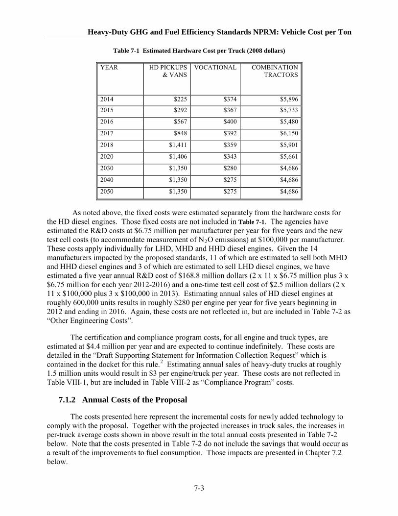
Heavy-Duty GHG and Fuel Efficiency Standards NPRM: Vehicle Cost per Ton
7-3
Table 7-1 Estimated Hardware Cost per Truck (2008 dollars)
YEAR HD PICKUPS & VANS
VOCATIONAL COMBINATION TRACTORS
2014 $225 $374 $5,896
2015 $292 $367 $5,733
2016 $567 $400 $5,480
2017 $848 $392 $6,150
2018 $1,411 $359 $5,901
2020 $1,406 $343 $5,661
2030 $1,350 $280 $4,686
2040 $1,350 $275 $4,686
2050 $1,350 $275 $4,686
As noted above, the fixed costs were estimated separately from the hardware costs for the HD diesel engines. Those fixed costs are not included in Table 7-1. The agencies have estimated the R&D costs at $6.75 million per manufacturer per year for five years and the new test cell costs (to accommodate measurement of N2
Table 7-2
O emissions) at $100,000 per manufacturer. These costs apply individually for LHD, MHD and HHD diesel engines. Given the 14 manufacturers impacted by the proposed standards, 11 of which are estimated to sell both MHD and HHD diesel engines and 3 of which are estimated to sell LHD diesel engines, we have estimated a five year annual R&D cost of $168.8 million dollars (2 x 11 x $6.75 million plus 3 x $6.75 million for each year 2012-2016) and a one-time test cell cost of $2.5 million dollars (2 x 11 x $100,000 plus 3 x $100,000 in 2013). Estimating annual sales of HD diesel engines at roughly 600,000 units results in roughly $280 per engine per year for five years beginning in 2012 and ending in 2016. Again, these costs are not reflected in, but are included in as “Other Engineering Costs”.
The certification and compliance program costs, for all engine and truck types, are estimated at $4.4 million per year and are expected to continue indefinitely. These costs are detailed in the “Draft Supporting Statement for Information Collection Request” which is contained in the docket for this rule.2
7.1.2 Annual Costs of the Proposal
Estimating annual sales of heavy-duty trucks at roughly 1.5 million units would result in $3 per engine/truck per year. These costs are not reflected in Table VIII-1, but are included in Table VIII-2 as “Compliance Program” costs.
The costs presented here represent the incremental costs for newly added technology to comply with the proposal. Together with the projected increases in truck sales, the increases in per-truck average costs shown in above result in the total annual costs presented in Table 7-2 below. Note that the costs presented in Table 7-2 do not include the savings that would occur as a result of the improvements to fuel consumption. Those impacts are presented in Chapter 7.2 below.
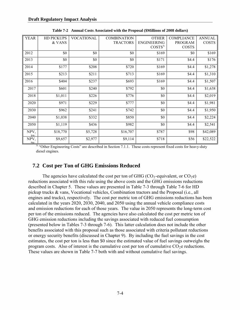
Draft Regulatory Impact Analysis
7-4
Table 7-2 Annual Costs Associated with the Proposal ($Millions of 2008 dollars)
YEAR HD PICKUPS & VANS
VOCATIONAL COMBINATION TRACTORS
OTHER ENGINEERING
COSTS
COMPLIANCE PROGRAM
COSTS A
ANNUAL COSTS
2012 $0 $0 $0 $169 $0 $169
2013 $0 $0 $0 $171 $4.4 $176
2014 $177 $208 $720 $169 $4.4 $1,278
2015 $213 $211 $713 $169 $4.4 $1,310
2016 $404 $237 $693 $169 $4.4 $1,507
2017 $601 $240 $792 $0 $4.4 $1,638
2018 $1,011 $226 $776 $0 $4.4 $2,019
2020 $971 $229 $777 $0 $4.4 $1,981
2030 $962 $241 $742 $0 $4.4 $1,950
2040 $1,038 $332 $850 $0 $4.4 $2,224
2050 $1,119 $436 $982 $0 $4.4 $2,541
NPV, 3%
$18,770 $5,728 $16,707 $787 $98 $42,089
NPV, 7%
$9,657 $2,977 $9,114 $718 $56 $22,522 A 7.1.1 “Other Engineering Costs” are described in Section . These costs represent fixed costs for heavy-duty
diesel engines.
7.2 Cost per Ton of GHG Emissions Reduced
The agencies have calculated the cost per ton of GHG (CO2-equivalent, or CO2
Table 7-3
e) reductions associated with this rule using the above costs and the GHG emissions reductions described in Chapter 5. These values are presented in through Table 7-6 for HD pickup trucks & vans, Vocational vehicles, Combination tractors and the Proposal (i.e., all engines and trucks), respectively. The cost per metric ton of GHG emissions reductions has been calculated in the years 2020, 2030, 2040, and 2050 using the annual vehicle compliance costs and emission reductions for each of those years. The value in 2050 represents the long-term cost per ton of the emissions reduced. The agencies have also calculated the cost per metric ton of GHG emission reductions including the savings associated with reduced fuel consumption (presented below in Tables 7-3 through 7-6). This latter calculation does not include the other benefits associated with this proposal such as those associated with criteria pollutant reductions or energy security benefits (discussed in Chapter 9). By including the fuel savings in the cost estimates, the cost per ton is less than $0 since the estimated value of fuel savings outweighs the program costs. Also of interest is the cumulative cost per ton of cumulative CO2
Table 7-7e reductions.
These values are shown in both with and without cumulative fuel savings.

Heavy-Duty GHG and Fuel Efficiency Standards NPRM: Vehicle Cost per Ton
7-5
Table 7-3 Annual Cost per Metric Ton of CO2
YEAR
e Reduced – HD Pickup Trucks & Vans (2008 dollars)
PROGRAM COST
FUEL SAVINGS
(POST-TAX)
CO2 COST PER TON
(WITHOUT FUEL
SAVINGS)
E REDUCED
COST PER TON (WITH
FUEL SAVINGS)
2020 $1,000 $1,000 4 $270 $0 2030 $1,000 $3,000 10 $100 -$200 2040 $1,000 $4,600 13 $70 -$270 2050 $1,100 $5,800 16 $70 -$290
Table 7-4 Annual Cost per Metric Ton of CO2
YEAR
e Reduced – Vocational Vehicles (2008 dollars)
PROGRAM COST
FUEL SAVINGS
(POST-TAX)
CO2 COST PER TON
(WITHOUT FUEL
SAVINGS)
E REDUCED
COST PER TON (WITH
FUEL SAVINGS)
2020 $200 $1,500 6 $30 -$220 2030 $200 $3,700 13 $20 -$280 2040 $300 $6,400 19 $20 -$320 2050 $400 $8,900 26 $20 -$330
Table 7-5 Annual Cost per Metric Ton of CO2
YEAR
e Reduced – Combination Tractors (2008 dollars)
PROGRAM COST
FUEL SAVINGS
(POST-TAX)
CO2 COST PER TON
(WITHOUT FUEL
SAVINGS)
E REDUCED
COST PER TON (WITH
FUEL SAVINGS)
2020 $800 $6,700 26 $30 -$230 2030 $700 $14,500 48 $10 -$280 2040 $800 $19,800 59 $10 -$320 2050 $1,000 $23,700 67 $10 -$340
Table 7-6 Annual Cost per Metric Ton of CO2
YEAR
e Reduced – Proposal (2008 dollars)
PROGRAM COST
FUEL SAVINGS
(POST-TAX)
CO2 COST PER TON
(WITHOUT FUEL
SAVINGS)
E REDUCED
COST PER TON (WITH
FUEL SAVINGS)
2020 $2,000 $9,300 35 $50 -$210 2030 $1,900 $21,200 71 $30 -$270 2040 $2,200 $30,800 91 $20 -$310 2050 $2,500 $38,400 109 $20 -$330

Draft Regulatory Impact Analysis
7-6
Table 7-7 Cumulative Cost per Cumulative Metric Ton of CO2
YEAR
e Reduced (2008 dollars)
PROGRAM COST
FUEL SAVINGS (POST-TAX)
CO2 COST PER TON (WITHOUT
FUEL SAVINGS)
E REDUCED
COST PER TON (WITH
FUEL SAVINGS)
2020 $12,100 $32,200 133 $90 -$150 2030 $31,300 $197,100 700 $40 -$240 2040 $52,300 $462,100 1,525 $30 -$270 2050 $76,200 $811,100 2,536 $30 -$290
7.3 Impacts of Reduction in Fuel Consumption
7.3.1 Gallons Reduced under the Proposal
The new CO2 standards will result in significant improvements in the fuel efficiency of affected trucks. Drivers of those trucks will see corresponding savings associated with reduced fuel expenditures. The agencies have estimated the impacts on fuel consumption for the tailpipe CO2 standards. To do this, fuel consumption is calculated using both current CO2 emission levels and the new CO2 standards. The difference between these estimates represents the net savings from the CO2
The expected impacts on fuel consumption are shown in
standards. Note that the total number of miles that vehicles are driven each year is different under each of the control case scenarios than in the reference case due to the “rebound effect,” which is discussed in Chapter 9. EPA also notes that drivers who drive more than our average estimates for vehicle miles traveled (VMT) will experience more fuel savings; drivers who drive less than our average VMT estimates will experience less fuel savings.
Table 7-8. The gallons shown in this table reflect impacts from the new CO2
Table 7-8 Fuel Consumption Reductions of the Proposal (Million gallons)
standards and include increased consumption resulting from the rebound effect.
GASOLINE DIESEL YEAR HD
PICKUPS & VANS
VOC COMB TOTAL HD
PICKUPS & VANS
VOC COMB TOTAL
2012 0.0 0.0 0.0 0.0 0.0 0.0 0.0 0.0 2013 0.0 0.0 0.0 0.0 0.0 0.0 0.0 0.0 2014 1.8 0.0 0.0 1.8 5.0 48 264 316 2015 5.2 0.0 0.0 5.2 12 93 519 624 2016 15 5.5 0.0 20 30 136 765 931 2017 31 11 0.0 42 57 221 1,115 1,393 2018 60 16 0.0 76 106 301 1,454 1,861 2020 114 26 0.0 140 199 445 2,079 2,723 2030 310 63 0.0 373 529 953 3,930 5,412 2040 421 75 0.0 496 715 1,483 4,805 7,004 2050 507 96 0.0 603 862 2,008 5,583 8,453

Heavy-Duty GHG and Fuel Efficiency Standards NPRM: Vehicle Cost per Ton
7-7
7.3.2 Monetized Fuel Savings
Using the fuel consumption estimates presented above, the agencies can calculate the monetized fuel savings associated with the proposed standards. To do this, reduced fuel consumption is multiplied in each year by the corresponding estimated average fuel price in that year, using the reference case taken from the AEO 2010. These estimates do not account for the significant uncertainty in future fuel prices; the monetized fuel savings will be understated if actual fuel prices are higher (or overstated if fuel prices are lower) than estimated. The Annual Energy Outlook (AEO) is a standard reference used by NHTSA and EPA and many other government agencies to estimate the projected price of fuel. This has been done using both the pre-tax and post-tax fuel prices. Since the post-tax fuel prices are the prices paid at fuel pumps, the fuel savings calculated using these prices represent the savings consumers would see. The pre-tax fuel savings are those savings that society would see. These results are shown in Table 7-9. Note that in Chapter 9, the overall benefits and costs of the rule are presented and, for that reason, only the pre-tax fuel savings are presented there.
Table 7-9 Estimated Monetized Fuel Savings ($Millions of 2008 dollars)
YEAR FUEL SAVINGS (PRE-TAX) FUEL SAVINGS (POST-TAX) 2014 $700 $800 2015 $1,400 $1,700 2016 $2,200 $2,700 2017 $3,600 $4,200 2018 $5,100 $5,900 2020 $8,100 $9,300 2030 $19,000 $21,200 2040 $28,100 $30,800 2050 $35,400 $38,400 NPV, 3% $352,300 $391,200 NPV, 7% $152,600 $170,600
7.4 Key Parameters Used in the Estimation of Costs and Fuel Savings
This section briefly presents some of the parameters used in generating costs and fuel savings associated with the proposal. Table 7-10 presents estimated sales of complying vehicles by calendar year. Table 7-11 presents VMT by age for both the reference and control cases where the control case includes rebound VMT. Table 7-12 presents AEO 2010 reference case fuel prices.
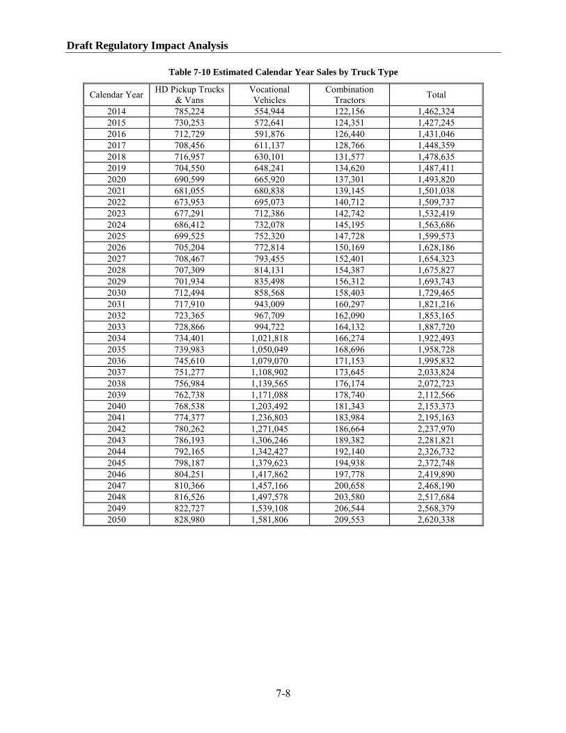
Draft Regulatory Impact Analysis
7-8
Table 7-10 Estimated Calendar Year Sales by Truck Type
Calendar Year HD Pickup Trucks & Vans
Vocational Vehicles
Combination Tractors Total
2014 785,224 554,944 122,156 1,462,324 2015 730,253 572,641 124,351 1,427,245 2016 712,729 591,876 126,440 1,431,046 2017 708,456 611,137 128,766 1,448,359 2018 716,957 630,101 131,577 1,478,635 2019 704,550 648,241 134,620 1,487,411 2020 690,599 665,920 137,301 1,493,820 2021 681,055 680,838 139,145 1,501,038 2022 673,953 695,073 140,712 1,509,737 2023 677,291 712,386 142,742 1,532,419 2024 686,412 732,078 145,195 1,563,686 2025 699,525 752,320 147,728 1,599,573 2026 705,204 772,814 150,169 1,628,186 2027 708,467 793,455 152,401 1,654,323 2028 707,309 814,131 154,387 1,675,827 2029 701,934 835,498 156,312 1,693,743 2030 712,494 858,568 158,403 1,729,465 2031 717,910 943,009 160,297 1,821,216 2032 723,365 967,709 162,090 1,853,165 2033 728,866 994,722 164,132 1,887,720 2034 734,401 1,021,818 166,274 1,922,493 2035 739,983 1,050,049 168,696 1,958,728 2036 745,610 1,079,070 171,153 1,995,832 2037 751,277 1,108,902 173,645 2,033,824 2038 756,984 1,139,565 176,174 2,072,723 2039 762,738 1,171,088 178,740 2,112,566 2040 768,538 1,203,492 181,343 2,153,373 2041 774,377 1,236,803 183,984 2,195,163 2042 780,262 1,271,045 186,664 2,237,970 2043 786,193 1,306,246 189,382 2,281,821 2044 792,165 1,342,427 192,140 2,326,732 2045 798,187 1,379,623 194,938 2,372,748 2046 804,251 1,417,862 197,778 2,419,890 2047 810,366 1,457,166 200,658 2,468,190 2048 816,526 1,497,578 203,580 2,517,684 2049 822,727 1,539,108 206,544 2,568,379 2050 828,980 1,581,806 209,553 2,620,338

Heavy-Duty GHG and Fuel Efficiency Standards NPRM: Vehicle Cost per Ton
7-9
Table 7-11 Annual Vehicle Miles Traveled by Age for the Reference and Control Cases
Vehicle Age
Reference Control
HD Pickup Trucks & Vans
Vocational Vehicles
Combination Tractors
HD Pickup Trucks & Vans
Vocational Vehicles
Combination Tractors
0 13,518 20,762 137,756 13,655 20,892 138,734 1 13,412 19,092 127,350 13,547 19,212 128,254 2 13,263 17,552 117,323 13,397 17,661 118,157 3 13,072 16,118 107,887 13,204 16,218 108,653 4 12,838 14,804 99,347 12,967 14,896 100,052 5 12,569 13,586 91,299 12,696 13,670 91,947 6 12,270 12,472 83,394 12,394 12,549 83,986 7 11,945 11,428 75,595 12,066 11,499 76,132 8 11,593 10,489 68,476 11,711 10,554 68,962 9 11,216 9,650 62,087 11,330 9,710 62,528
10 10,817 8,936 56,300 10,926 8,991 56,700 11 10,405 8,263 51,145 10,510 8,313 51,508 12 9,986 7,659 46,367 10,086 7,705 46,697 13 9,566 7,126 41,939 9,663 7,170 42,237 14 9,152 6,626 37,762 9,244 6,667 38,030 15 8,747 6,168 34,079 8,835 6,205 34,321 16 8,355 5,747 30,738 8,439 5,782 30,956 17 8,037 5,368 27,800 8,118 5,401 27,998 18 7,741 5,050 25,019 7,820 5,080 25,197 19 7,470 4,741 22,587 7,546 4,769 22,748 20 7,227 4,436 20,369 7,300 4,463 20,514 21 7,020 4,202 18,486 7,090 4,227 18,618 22 6,853 3,972 16,700 6,922 3,995 16,818 23 6,733 3,773 15,078 6,801 3,795 15,185 24 6,669 3,581 13,619 6,736 3,603 13,716 25 6,661 3,397 12,294 6,728 3,417 12,381 26 6,707 3,239 11,101 6,775 3,258 11,179 27 6,765 3,118 10,044 6,833 3,136 10,116 28 6,824 2,967 9,089 6,893 2,984 9,153 29 6,884 2,853 8,202 6,954 2,869 8,260 30 6,946 2,766 7,417 7,016 2,782 7,470

Draft Regulatory Impact Analysis
7-10
Table 7-12 AEO 2010 Reference Case Fuel Prices (2008 dollars/gallon)
Pre-Tax Post-Tax Vehicle Age Gasoline Diesel Gasoline Diesel
2014 $2.61 $2.61 $3.02 $3.05 2015 $2.67 $2.71 $3.07 $3.14 2016 $2.74 $2.82 $3.14 $3.24 2017 $2.81 $2.90 $3.20 $3.32 2018 $2.86 $2.99 $3.25 $3.41 2019 $2.90 $3.05 $3.29 $3.47 2020 $2.95 $3.09 $3.34 $3.51 2021 $2.98 $3.12 $3.37 $3.53 2022 $3.03 $3.17 $3.41 $3.58 2023 $3.06 $3.20 $3.44 $3.60 2024 $3.08 $3.21 $3.45 $3.61 2025 $3.12 $3.25 $3.49 $3.65 2026 $3.16 $3.29 $3.53 $3.68 2027 $3.20 $3.33 $3.57 $3.71 2028 $3.25 $3.37 $3.62 $3.76 2029 $3.30 $3.43 $3.66 $3.81 2030 $3.32 $3.46 $3.68 $3.83 2031 $3.36 $3.52 $3.72 $3.89 2032 $3.41 $3.58 $3.77 $3.94 2033 $3.45 $3.62 $3.80 $3.99 2034 $3.49 $3.68 $3.85 $4.04 2035 $3.56 $3.75 $3.91 $4.11 2036 $3.59 $3.76 $3.94 $4.12 2037 $3.62 $3.78 $3.97 $4.13 2038 $3.65 $3.79 $3.99 $4.14 2039 $3.68 $3.81 $4.02 $4.15 2040 $3.71 $3.82 $4.05 $4.17 2041 $3.74 $3.83 $4.08 $4.18 2042 $3.77 $3.85 $4.11 $4.19 2043 $3.80 $3.86 $4.13 $4.20 2044 $3.83 $3.88 $4.16 $4.21 2045 $3.86 $3.89 $4.19 $4.23 2046 $3.89 $3.91 $4.22 $4.24 2047 $3.92 $3.92 $4.25 $4.25 2048 $3.95 $3.94 $4.28 $4.26 2049 $3.98 $3.95 $4.31 $4.28 2050 $4.01 $3.97 $4.34 $4.29

Heavy-Duty GHG and Fuel Efficiency Standards NPRM: Vehicle Cost per Ton
7-11
1 Light-Duty Vehicle Greenhouse Gas Emission Standards and Corporate Average Fuel Economy Standards; Final Rule 75 Fed. Reg. 25323 (May 7, 2010).
References
2 “Draft Supporting Statement for Information Collection Request,” Control of Greenhouse Gas Emissions from New Motor Vehicles: Proposed Heavy-Duty Engine and Vehicle Standards, EPA ICR Tracking Number 2394.01.

Heavy-Duty GHG and Fuel Efficiency Standards NPRM: Environmental and Health Impacts
8-1
Chapter 8: Health and Environmental Impacts 8.1 Health and Environmental Effects of Non-GHG Pollutants
8.1.1 Health Effects Associated with Exposure to Non-GHG Pollutants
In this section we will discuss the health effects associated with non-GHG pollutants, specifically: particulate matter, ozone, nitrogen oxides (NOX), sulfur oxides (SOX
8.1.1.1 Background on Particulate Matter
), carbon monoxide and air toxics. These pollutants would not be directly regulated by the standards, but the standards would affect emissions of these pollutants and precursors. Reductions in these pollutants would be co-benefits of the final rulemaking (that is, benefits in addition to the benefits of reduced GHGs).
Particulate matter (PM) is a generic term for a broad class of chemically and physically diverse substances. It can be principally characterized as discrete particles that exist in the condensed (liquid or solid) phase spanning several orders of magnitude in size. Since 1987, EPA has delineated that subset of inhalable particles small enough to penetrate to the thoracic region (including the tracheobronchial and alveolar regions) of the respiratory tract (referred to as thoracic particles). Current National Ambient Air Quality Standards (NAAQS) use PM2.5 as the indicator for fine particles (with PM2.5 referring to particles with a nominal mean aerodynamic diameter less than or equal to 2.5 µm), and use PM10 as the indicator for purposes of regulating the coarse fraction of PM10 (referred to as thoracic coarse particles or coarse-fraction particles; generally including particles with a nominal mean aerodynamic diameter greater than 2.5 µm and less than or equal to 10 µm, or PM10-2.5
Particles span many sizes and shapes and consist of numerous different chemicals. Particles originate from sources and are also formed through atmospheric chemical reactions; the former are often referred to as “primary” particles, and the latter as “secondary” particles. In addition, there are also physical, non-chemical reaction mechanisms that contribute to secondary particles. Particle pollution also varies by time of year and location and is affected by several weather-related factors, such as temperature, clouds, humidity, and wind. A further layer of complexity comes from a particle’s ability to shift between solid/liquid and gaseous phases, which is influenced by concentration, meteorology, and temperature.
). Ultrafine particles (UFPs) are a subset of fine particles, generally less than 100 nanometers (0.1 μm) in aerodynamic diameter.
Fine particles are produced primarily by combustion processes and by transformations of gaseous emissions (e.g., SOX, NOX and volatile organic compounds (VOCs)) in the atmosphere. The chemical and physical properties of PM2.5 may vary greatly with time, region, meteorology and source category. Thus, PM2.5 may include a complex mixture of different chemicals including sulfates, nitrates, organic compounds, elemental carbon and metal compounds. These particles can remain in the atmosphere for days to weeks and travel through the atmosphere hundreds to thousands of kilometers.1

Draft Regulatory Impact Analysis
8-2
8.1.1.2 Particulate Matter Health Effects
This section provides a summary of the health effects associated with exposure to ambient concentrations of PM.A The information in this section is based on the information and conclusions in the Integrated Science Assessment (ISA) for Particulate Matter (December 2009) prepared by EPA’s Office of Research and Development (ORD).B
The ISA concludes that ambient concentrations of PM are associated with a number of adverse health effects.
C The ISA characterizes the weight of evidence for different health effects associated with three PM size ranges: PM2.5, PM10-2.5
8.1.1.2.1 Effects Associated with Short-term Exposure to PM
, and UFPs. The discussion below highlights the ISA’s conclusions pertaining to these three size fractions of PM, considering variations in both short-term and long-term exposure periods.
The ISA concludes that cardiovascular effects and all-cause cardiovascular- and respiratory-related mortality are causally associated with short-term exposure to PM
2.5
2.5.2 It also concludes that respiratory effects are likely to be causally associated with short-term exposure to PM2.5
8.1.1.2.2 Effects Associated with Long-term Exposure to PM
, including respiratory emergency department (ED) visits and hospital admissions for chronic obstructive pulmonary disease (COPD), respiratory infections, and asthma; and exacerbation of respiratory symptoms in asthmatic children.
The ISA concludes that there are causal associations between long-term exposure to PM
2.5
2.5 and cardiovascular effects, such as the development/progression of cardiovascular disease (CVD), and premature mortality, particularly from cardiopulmonary causes.3 It also concludes that long-term exposure to PM2.5 is likely to be causally associated with respiratory effects, such as reduced lung function growth, increased respiratory symptoms, and asthma development. The ISA characterizes the evidence as suggestive of a causal relationship for associations between long-term PM2.5 exposure and reproductive and developmental outcomes, such as low birth weight and infant mortality. It also characterizes the evidence as suggestive of a causal relationship between PM2.5
8.1.1.2.3 Effects Associated with PM
and cancer incidence, mutagenicity, and genotoxicity.
The ISA summarizes evidence related to short-term exposure to PM
10-2.5
10-2.5. PM10-2.5 is the fraction of PM10 particles that is larger than PM2.5.4
A Personal exposure includes contributions from many different types of particles, from many sources, and in many different environments. Total personal exposure to PM includes both ambient and nonambient components; and both components may contribute to adverse health effects.
The ISA concludes that available evidence
B The ISA is available at http://cfpub.epa.gov/ncea/cfm/recordisplay.cfm?deid=216546 C The ISA evaluates the health evidence associated with different health effects, assigning one of five “weight of evidence” determinations: causal relationship, likely to be a causal relationship, suggestive of a causal relationship, inadequate to infer a causal relationship, and not likely to be a causal relationship. For definitions of these levels of evidence, please refer to Section 1.5 of the ISA.

Heavy-Duty GHG and Fuel Efficiency Standards NPRM: Environmental and Health Impacts
8-3
is suggestive of a causal relationship between short-term exposures to PM10-2.5 and cardiovascular effects, such as hospitalizations for ischemic heart disease. It also concludes that the available evidence is suggestive of a causal relationship between short-term exposures to PM10-2.5 and respiratory effects, including respiratory-related ED visits and hospitalizations and pulmonary inflammation. The ISA also concludes that the available literature suggests a causal relationship between short-term exposures to PM10-2.5 and mortality. Data are inadequate to draw conclusions regarding health effects associated with long-term exposure to PM10-2.5.5
8.1.1.2.4 Effects Associated with Ultrafine Particles
The ISA concludes that the evidence is suggestive of a causal relationship between short-term exposures to UFPs and cardiovascular effects, including changes in heart rhythm and vasomotor function (the ability of blood vessels to expand and contract).6
The ISA also concludes that there is suggestive evidence of a causal relationship between short-term UFP exposure and respiratory effects. The types of respiratory effects examined in epidemiologic studies include respiratory symptoms and asthma hospital admissions, the results of which are not entirely consistent. There is evidence from toxicological and controlled human exposure studies that exposure to UFPs may increase lung inflammation and produce small asymptomatic changes in lung function. Data are inadequate to draw conclusions regarding health effects associated with long-term exposure to UFPs.
7
8.1.1.3 Background on Ozone
Ground-level ozone pollution is typically formed by the reaction of VOCs and NOX
The science of ozone formation, transport, and accumulation is complex. Ground-level ozone is produced and destroyed in a cyclical set of chemical reactions, many of which are sensitive to temperature and sunlight. When ambient temperatures and sunlight levels remain high for several days and the air is relatively stagnant, ozone and its precursors can build up and result in more ozone than typically occurs on a single high-temperature day. Ozone can be transported hundreds of miles downwind of precursor emissions, resulting in elevated ozone levels even in areas with low VOC or NO
in the lower atmosphere in the presence of sunlight. These pollutants, often referred to as ozone precursors, are emitted by many types of pollution sources such as highway and nonroad motor vehicles and engines, power plants, chemical plants, refineries, makers of consumer and commercial products, industrial facilities, and smaller area sources.
X
The highest levels of ozone are produced when both VOC and NO
emissions.
X emissions are present in significant quantities on clear summer days. Relatively small amounts of NOX enable ozone to form rapidly when VOC levels are relatively high, but ozone production is quickly limited by removal of the NOX. Under these conditions NOX reductions are highly effective in reducing ozone while VOC reductions have little effect. Such conditions are called “NOX-limited.” Because the contribution of VOC emissions from biogenic (natural) sources to local ambient ozone concentrations can be significant, even some areas where man-made VOC emissions are relatively low can be NOX-limited.
Draft Regulatory Impact Analysis
8-4
Ozone concentrations in an area also can be lowered by the reaction of nitric oxide (NO) with ozone, forming nitrogen dioxide (NO2); as the air moves downwind and the cycle continues, the NO2 forms additional ozone. The importance of this reaction depends, in part, on the relative concentrations of NOX, VOC, and ozone, all of which change with time and location. When NOX levels are relatively high and VOC levels relatively low, NOX forms inorganic nitrates (i.e., particles) but relatively little ozone. Such conditions are called “VOC-limited.” Under these conditions, VOC reductions are effective in reducing ozone, but NOX reductions can actually increase local ozone under certain circumstances. Even in VOC-limited urban areas, NOX reductions are not expected to increase ozone levels if the NOX reductions are sufficiently large. Rural areas are usually NOX-limited, due to the relatively large amounts of biogenic VOC emissions in such areas. Urban areas can be either VOC- or NOX
8.1.1.4 Ozone Health Effects
-limited, or a mixture of both, in which ozone levels exhibit moderate sensitivity to changes in either pollutant.
Exposure to ambient ozone contributes to a wide range of adverse health effects.D These health effects are well documented and are critically assessed in the EPA ozone air quality criteria document (ozone AQCD) and EPA staff paper.8,9
Ozone-related health effects include lung function decrements, respiratory symptoms, aggravation of asthma, increased hospital and emergency room visits, increased asthma medication usage, and a variety of other respiratory effects. Cellular-level effects, such as inflammation of lungs, have been documented as well. In addition, there is suggestive evidence of a contribution of ozone to cardiovascular-related morbidity and highly suggestive evidence that short-term ozone exposure directly or indirectly contributes to non-accidental and cardiopulmonary-related mortality, but additional research is needed to clarify the underlying mechanisms causing these effects. In a recent report on the estimation of ozone-related premature mortality published by the National Research Council (NRC), a panel of experts and reviewers concluded that short-term exposure to ambient ozone is likely to contribute to premature deaths and that ozone-related mortality should be included in estimates of the health benefits of reducing ozone exposure.
We are relying on the data and conclusions in the ozone AQCD and staff paper, regarding the health effects associated with ozone exposure.
10
Based on a large number of scientific studies, EPA has identified several key health effects associated with exposure to levels of ozone found today in many areas of the country.
People who appear to be more susceptible to effects associated with exposure to ozone include children, asthmatics and the elderly. Those with greater exposures to ozone, for instance due to time spent outdoors (e.g., children and outdoor workers), are also of concern.
D Human exposure to ozone varies over time due to changes in ambient ozone concentration and because people move between locations which have notable different ozone concentrations. Also, the amount of ozone delivered to the lung is not only influenced by the ambient concentrations but also by the individuals breathing route and rate.

Heavy-Duty GHG and Fuel Efficiency Standards NPRM: Environmental and Health Impacts
8-5
Short-term (1 to 3 hours) and prolonged exposures (6 to 8 hours) to ambient ozone concentrations have been linked to lung function decrements, respiratory symptoms, increased hospital admissions and emergency room visits for respiratory problems.11, 12, 13, 14, 15, 16 Repeated exposure to ozone can increase susceptibility to respiratory infection and lung inflammation and can aggravate preexisting respiratory diseases, such as asthma.17, 18, 19, 20, 21 Repeated exposure to sufficient concentrations of ozone can also cause inflammation of the lung, impairment of lung defense mechanisms, and possibly irreversible changes in lung structure, which over time could affect premature aging of the lungs and/or the development of chronic respiratory illnesses, such as emphysema and chronic bronchitis.22, 23, 24, 25
Children and adults who are outdoors and active during the summer months, such as construction workers, are among those most at risk of elevated ozone exposures.
26 Children and outdoor workers tend to have higher ozone exposure because they typically are active outside, working, playing and exercising, during times of day and seasons (e.g., the summer) when ozone levels are highest.27 For example, summer camp studies in the Eastern United States and Southeastern Canada have reported statistically significant reductions in lung function in children who are active outdoors.28, 29, 30, 31, 32, 33, 34, 35 Further, children are more at risk of experiencing health effects from ozone exposure than adults because their respiratory systems are still developing. These individuals (as well as people with respiratory illnesses, such as asthma, especially asthmatic children) can experience reduced lung function and increased respiratory symptoms, such as chest pain and cough, when exposed to relatively low ozone levels during prolonged periods of moderate exertion.36, 37, 38, 39
8.1.1.5 Background on Nitrogen Oxides and Sulfur Oxides
Sulfur dioxide (SO2), a member of the sulfur oxide (SOX) family of gases, is formed from burning fuels containing sulfur (e.g., coal or oil), extracting gasoline from oil, or extracting metals from ore. Nitrogen dioxide (NO2) is a member of the nitrogen oxide (NOX) family of gases. Most NO2 is formed in the air through the oxidation of nitric oxide (NO) emitted when fuel is burned at a high temperature. SO2 and NO2
8.1.1.2
can dissolve in water droplets and further oxidize to form sulfuric and nitric acid which react with ammonia to form sulfates and nitrates, both of which are important components of ambient PM. The health effects of ambient PM are discussed in Section . NOX
8.1.1.4 along with non-methane hydrocarbons (NMHC) are the two
major precursors of ozone. The health effects of ozone are covered in Section .
8.1.1.6 Health Effects of SO
This section provides an overview of the health effects associated with SO
2
2. Additional information on the health effects of SO2 can be found in the EPA Integrated Science Assessment for Sulfur Oxides.40 Following an extensive evaluation of health evidence from epidemiologic and laboratory studies, the U.S. EPA has concluded that there is a causal relationship between respiratory health effects and short-term exposure to SO2. The immediate effect of SO2 on the respiratory system in humans is bronchoconstriction. Asthmatics are more sensitive to the effects of SO2 likely resulting from preexisting inflammation associated with this disease. In laboratory studies involving controlled human exposures to SO2, respiratory effects have consistently been observed following 5-10 min exposures at SO2 concentrations ≥ 0.4 ppm in asthmatics engaged in moderate to heavy levels of exercise, with more limited evidence of respiratory effects among

Draft Regulatory Impact Analysis
8-6
exercising asthmatics exposed to concentrations as low as 0.2-0.3 ppm. A clear concentration-response relationship has been demonstrated in these studies following exposures to SO2
In epidemiologic studies, respiratory effects have been observed in areas where the mean 24-hour SO
at concentrations between 0.2 and 1.0 ppm, both in terms of increasing severity of respiratory symptoms and decrements in lung function, as well as the percentage of asthmatics adversely affected.
2 levels range from 1 to 30 ppb, with maximum 1 to 24-hour average SO2 values ranging from 12 to 75 ppb. Important new multicity studies and several other studies have found an association between 24-hour average ambient SO2 concentrations and respiratory symptoms in children, particularly those with asthma. Generally consistent associations also have been observed between ambient SO2 concentrations and emergency department visits and hospitalizations for all respiratory causes, particularly among children and older adults (≥ 65 years), and for asthma. A limited subset of epidemiologic studies have examined potential confounding by copollutants using multipollutant regression models. These analyses indicate that although copollutant adjustment has varying degrees of influence on the SO2 effect estimates, the effect of SO2 on respiratory health outcomes appears to be generally robust and independent of the effects of gaseous and particulate copollutants, suggesting that the observed effects of SO2
Consistent associations between short-term exposure to SO
on respiratory endpoints occur independent of the effects of other ambient air pollutants.
2 and mortality have been observed in epidemiologic studies, with larger effect estimates reported for respiratory mortality than for cardiovascular mortality. While this finding is consistent with the demonstrated effects of SO2 on respiratory morbidity, uncertainty remains with respect to the interpretation of these associations due to potential confounding by various copollutants. The U.S. EPA has therefore concluded that the overall evidence is suggestive of a causal relationship between short-term exposure to SO2 and mortality. Significant associations between short-term exposure to SO2 and emergency department visits and hospital admissions for cardiovascular diseases have also been reported. However, these findings have been inconsistent across studies and do not provide adequate evidence to infer a causal relationship between SO2
8.1.1.7 Health Effects of NO
exposure and cardiovascular morbidity.
Information on the health effects of NO
2
2 can be found in the EPA Integrated Science Assessment (ISA) for Nitrogen Oxides.41 The EPA has concluded that the findings of epidemiologic, controlled human exposure, and animal toxicological studies provide evidence that is sufficient to infer a likely causal relationship between respiratory effects and short-term NO2 exposure. The ISA concludes that the strongest evidence for such a relationship comes from epidemiologic studies of respiratory effects including symptoms, emergency department visits, and hospital admissions. The ISA also draws two broad conclusions regarding airway responsiveness following NO2 exposure. First, the ISA concludes that NO2 exposure may enhance the sensitivity to allergen-induced decrements in lung function and increase the allergen-induced airway inflammatory response following 30-minute exposures of asthmatics to NO2 concentrations as low as 0.26 ppm. In addition, small but significant increases in non-specific airway hyperresponsiveness were reported following 1-hour exposures of asthmatics to

Heavy-Duty GHG and Fuel Efficiency Standards NPRM: Environmental and Health Impacts
8-7
0.1 ppm NO2. Second, exposure to NO2 has been found to enhance the inherent responsiveness of the airway to subsequent nonspecific challenges in controlled human exposure studies of asthmatic subjects. Enhanced airway responsiveness could have important clinical implications for asthmatics since transient increases in airway responsiveness following NO2 exposure have the potential to increase symptoms and worsen asthma control. Together, the epidemiologic and experimental data sets form a plausible, consistent, and coherent description of a relationship between NO2
Although the weight of evidence supporting a causal relationship is somewhat less certain than that associated with respiratory morbidity, NO
exposures and an array of adverse health effects that range from the onset of respiratory symptoms to hospital admission.
2
8.1.1.8 Health Effects of Carbon Monoxide
has also been linked to other health endpoints. These include all-cause (nonaccidental) mortality, hospital admissions or emergency department visits for cardiovascular disease, and decrements in lung function growth associated with chronic exposure.
Information on the health effects of carbon monoxide (CO) can be found in the EPA Integrated Science Assessment (ISA) for Carbon Monoxide.42 The ISA concludes that ambient concentrations of CO are associated with a number of adverse health effects.E This section provides a summary of the health effects associated with exposure to ambient concentrations of CO.F
Human clinical studies of subjects with coronary artery disease show a decrease in the time to onset of exercise-induced angina (chest pain) and electrocardiogram changes following CO exposure. In addition, epidemiologic studies show associations between short-term CO exposure and cardiovascular morbidity, particularly increased emergency room visits and hospital admissions for coronary heart disease (including ischemic heart disease, myocardial infarction, and angina). Some epidemiologic evidence is also available for increased hospital admissions and emergency room visits for congestive heart failure and cardiovascular disease as a whole. The ISA concludes that a causal relationship is likely to exist between short-term exposures to CO and cardiovascular morbidity. It also concludes that available data are inadequate to conclude that a causal relationship exists between long-term exposures to CO and cardiovascular morbidity.
Animal studies show various neurological effects with in-utero CO exposure. Controlled human exposure studies report inconsistent neural and behavioral effects following low-level CO
E The ISA evaluates the health evidence associated with different health effects, assigning one of five “weight of evidence” determinations: causal relationship, likely to be a causal relationship, suggestive of a causal relationship, inadequate to infer a causal relationship, and not likely to be a causal relationship. For definitions of these levels of evidence, please refer to Section 1.6 of the ISA. F Personal exposure includes contributions from many sources, and in many different environments. Total personal exposure to CO includes both ambient and nonambient components; and both components may contribute to adverse health effects.

Draft Regulatory Impact Analysis
8-8
exposures. The ISA concludes the evidence is suggestive of a causal relationship with both short- and long-term exposure to CO and central nervous system effects.
A number of epidemiologic and animal toxicological studies cited in the ISA have evaluated associations between CO exposure and birth outcomes such as preterm birth or cardiac birth defects. The epidemiologic studies provide limited evidence of a CO-induced effect on preterm births and birth defects, with weak evidence for a decrease in birth weight. Animal toxicological studies have found associations between perinatal CO exposure and decrements in birth weight, as well as other developmental outcomes. The ISA concludes these studies are suggestive of a causal relationship between long-term exposures to CO and developmental effects and birth outcomes.
Epidemiologic studies provide evidence of effects on respiratory morbidity such as changes in pulmonary function, respiratory symptoms, and hospital admissions associated with ambient CO concentrations. A limited number of epidemiologic studies considered copollutants such as ozone, SO2
Finally, the ISA concludes that the epidemiologic evidence is suggestive of a causal relationship between short-term exposures to CO and mortality. Epidemiologic studies provide evidence of an association between short-term exposure to CO and mortality, but limited evidence is available to evaluate cause-specific mortality outcomes associated with CO exposure. In addition, the attenuation of CO risk estimates which was often observed in copollutant models contributes to the uncertainty as to whether CO is acting alone or as an indicator for other combustion-related pollutants. The ISA also concludes that there is not likely to be a causal relationship between relevant long-term exposures to CO and mortality.
, and PM in two-pollutant models and found that CO risk estimates were generally robust, although this limited evidence makes it difficult to disentangle effects attributed to CO itself from those of the larger complex air pollution mixture. Controlled human exposure studies have not extensively evaluated the effect of CO on respiratory morbidity. Animal studies at levels of 50-100 ppm CO show preliminary evidence of altered pulmonary vascular remodeling and oxidative injury. The ISA concludes that the evidence is suggestive of a causal relationship between short-term CO exposure and respiratory morbidity, and inadequate to conclude that a causal relationship exists between long-term exposure and respiratory morbidity.
8.1.1.9 Health Effects of Air Toxics
Motor vehicle emissions contribute to ambient levels of air toxics known or suspected as human or animal carcinogens, or that have noncancer health effects. The population experiences an elevated risk of cancer and other noncancer health effects from exposure to air toxics.43 These compounds include, but are not limited to, benzene, 1,3-butadiene, formaldehyde, acetaldehyde, acrolein, diesel particulate matter and exhaust organic gases, polycyclic organic matter (POM), and naphthalene. These compounds were identified as national or regional risk drivers in past National-scale Air Toxics Assessments (NATA) and have significant inventory contributions from mobile sources. Although the 2002 NATA did not quantify cancer risks associated with exposure to diesel exhaust, EPA has concluded that diesel exhaust ranks with the other emissions that the 2002 NATA suggests pose the greatest relative risk. According to NATA for 2002, mobile sources were responsible for 47 percent of outdoor toxic emissions, over 50 percent of the cancer risk, and over 80 percent of the noncancer hazard. Data from the 2002

Heavy-Duty GHG and Fuel Efficiency Standards NPRM: Environmental and Health Impacts
8-9
National Emissions Inventory (NEI), which is the basis for NATA, show that thirty percent of national diesel PM emissions are attributable to heavy-duty vehicles.44
Noncancer health effects can result from chronic,
G subchronic,H or acuteI inhalation exposures to air toxics, and include neurological, cardiovascular, liver, kidney, and respiratory effects as well as effects on the immune and reproductive systems. According to the 2002 NATA, nearly the entire U.S. population was exposed to an average concentration of air toxics that has the potential for adverse noncancer respiratory health effects. This will continue to be the case in 2030, even though toxics concentrations will be lower.45
The NATA modeling framework has a number of limitations which prevent its use as the sole basis for setting regulatory standards. These limitations and uncertainties are discussed on the 2002 NATA website.
46
8.1.1.9.1 Diesel Exhaust PM
Even so, this modeling framework is very useful in identifying air toxic pollutants and sources of greatest concern, setting regulatory priorities, and informing the decision making process.
Heavy-duty diesel engines emit diesel exhaust (DE), a complex mixture comprised of carbon dioxide, oxygen, nitrogen, water vapor, carbon monoxide, nitrogen compounds, sulfur compounds and numerous low-molecular-weight hydrocarbons. A number of these gaseous hydrocarbon components are individually known to be toxic including aldehydes, benzene and 1,3-butadiene. The diesel particulate matter (DPM) present in diesel exhaust consists of fine particles (< 2.5µm), including a subgroup with a large number of ultrafine particles (< 0.1 µm). These particles have large surface areas which make them an excellent medium for adsorbing organics, and their small size makes them highly respirable and able to deposit deep in the lung. Diesel PM contains small quantities of numerous mutagenic and carcinogenic compounds associated with the particles (and also organic gases). In addition, while toxic trace metals emitted by heavy-duty diesel engines represent a very small portion of the national emissions of metals (less than one percent) and are a small portion of diesel PM (generally much less than one percent of diesel PM), we note that several trace metals of potential toxicological significance and persistence in the environment are emitted by diesel engines. These trace metals include chromium, manganese, mercury and nickel. In addition, small amounts of dioxins have been measured in highway engine diesel exhaust, some of which may partition into the particulate phase. Dioxins are a major health concern but diesel engines are a minor contributor to overall dioxin emissions.
G Chronic exposure is defined in the glossary of the Integrated Risk Information (IRIS) database (http://www.epa.gov/iris) as repeated exposure by the oral, dermal, or inhalation route for more than approximately 10% of the life span in humans (more than approximately 90 days to 2 years in typically used laboratory animal species). H Defined in the IRIS database as exposure to a substance spanning approximately 10% of the lifetime of an organism. I Defined in the IRIS database as exposure by the oral, dermal, or inhalation route for 24 hours or less.

Draft Regulatory Impact Analysis
8-10
Diesel exhaust varies significantly in chemical composition and particle sizes between different engine types (heavy-duty, light-duty), engine operating conditions (idle, accelerate, decelerate), and fuel formulations (high/low sulfur fuel). 47
A number of health studies have been conducted regarding diesel exhaust. These include epidemiologic studies of lung cancer in groups of workers and animal studies focusing on non-cancer effects specific to diesel exhaust exposure. Diesel exhaust PM (including the associated organic compounds which are generally high molecular weight hydrocarbon types but not the more volatile gaseous hydrocarbon compounds) is generally used as a surrogate measure for diesel exhaust.
Also, there are emission differences between on-road and nonroad engines because the nonroad engines are generally of older technology. After being emitted, diesel exhaust undergoes dilution as well as chemical and physical changes in the atmosphere. The lifetime for some of the compounds present in diesel exhaust ranges from hours to days.
8.1.1.9.1.1 Potential Cancer Effects of Exposure to Diesel Exhaust
Exposure to diesel exhaust is of specific concern because it has been judged by EPA to pose a lung cancer hazard for humans at environmental levels of exposure.
EPA’s 2002 final “Health Assessment Document for Diesel Engine Exhaust” (the EPA Diesel HAD) classified exposure to diesel exhaust as likely to be carcinogenic to humans by inhalation at environmental exposures, in accordance with the revised draft 1996/1999 EPA cancer guidelines.48,49 In accordance with earlier EPA guidelines, exposure to diesel exhaust would similarly be classified as probably carcinogenic to humans (Group B1).50,51 A number of other agencies (National Institute for Occupational Safety and Health, the International Agency for Research on Cancer, the World Health Organization, California EPA, and the U.S. Department of Health and Human Services) have made similar classifications.52, 53,54,55,56 The Health Effects Institute has prepared numerous studies and reports on the potential carcinogenicity of exposure to diesel exhaust.57,58,59
More specifically, the EPA Diesel HAD states that the conclusions of the document apply to diesel exhaust in use today including both on-road and nonroad engines. The EPA Diesel HAD acknowledges that the studies were done on engines with generally older technologies and that “there have been changes in the physical and chemical composition of some DE [diesel exhaust] emissions (onroad vehicle emissions) over time, though there is no definitive information to show that the emission changes portend significant toxicological changes.”
For the Diesel HAD, EPA reviewed 22 epidemiologic studies on the subject of the carcinogenicity of exposure to diesel exhaust in various occupations, finding increased lung cancer risk, although not always statistically significant, in 8 out of 10 cohort studies and 10 out of 12 case-control studies which covered several industries. Relative risk for lung cancer, associated with exposure, ranged from 1.2 to 1.5, although a few studies show relative risks as high as 2.6. Additionally, the Diesel HAD also relied on two independent meta-analyses, which examined 23 and 30 occupational studies respectively, and found statistically significant increases of 1.33 to 1.47 in smoking-adjusted relative lung cancer risk associated with diesel exhaust. These meta-analyses demonstrate the effect of pooling many studies and in this case

Heavy-Duty GHG and Fuel Efficiency Standards NPRM: Environmental and Health Impacts
8-11
show the positive relationship between diesel exhaust exposure and lung cancer across a variety of diesel exhaust-exposed occupations.60,61,62
EPA generally derives cancer unit risk estimates to calculate population risk more precisely from exposure to carcinogens. In the simplest terms, the cancer unit risk is the increased risk associated with average lifetime exposure of 1 µg/m
3
In the absence of a cancer unit risk, the Diesel HAD sought to provide additional insight into the significance of the diesel exhaust-cancer hazard by estimating possible ranges of risk that might be present in the population. An exploratory analysis was used to characterize a possible risk range by comparing a typical environmental exposure level for highway diesel sources to a selected range of occupational exposure levels. The occupationally observed risks were then proportionally scaled according to the exposure ratios to obtain an estimate of the possible environmental risk. If the occupational and environmental exposures are similar, the environmental risk would approach the risk seen in the occupational studies whereas a much higher occupational exposure indicates that the environmental risk is lower than the occupational risk. A comparison of environmental and occupational exposures showed that for certain occupations the exposures are similar to environmental exposures while, for others, they differ by a factor of about 200 or more.
. EPA concluded in the Diesel HAD that it is not currently possible to calculate a cancer unit risk for diesel exhaust due to a variety of factors that limit the current studies, such as a lack of standard exposure metric for diesel exhaust and the absence of quantitative exposure characterization in retrospective studies.
A number of calculations are involved in the exploratory analysis of a possible risk range, and these can be seen in the EPA Diesel HAD. The outcome was that environmental risks from diesel exhaust exposure could range from a low of 10-4 to 10-5 to as high as 10-3, reflecting the range of occupational exposures that could be associated with the relative and absolute risk levels observed in the occupational studies. Because of uncertainties, the analysis acknowledged that the risks could be lower than 10-4 or 10-5
As mentioned in Section
, and a zero risk from diesel exhaust exposure was not ruled out.
8.1.1.9, EPA recently assessed air toxic emissions and their associated risk (the National-Scale Air Toxics Assessment or NATA for 2002), and we concluded that diesel exhaust ranks with other emissions that the national-scale assessment suggests pose the greatest relative risk.63
In summary, even though EPA does not have a specific carcinogenic potency with which to accurately estimate the carcinogenic impact of exposure to diesel exhaust, the likely hazard to humans together with the potential for significant environmental risks leads us to conclude that diesel exhaust emissions from heavy-duty diesel engines present public health issues of concern to this proposal.
This national assessment estimates average population inhalation exposures to DPM for nonroad as well as on-highway sources. These are the sum of ambient levels in various locations weighted by the amount of time people spend in each of the locations.

Draft Regulatory Impact Analysis
8-12
8.1.1.9.1.2 Other Health Effects of Exposure to Diesel Exhaust
Noncancer health effects of acute and chronic exposure to diesel exhaust emissions are also of concern to the EPA. The Diesel HAD established an inhalation Reference Concentration (RfC) specifically based on animal studies of diesel exhaust exposure. An RfC is defined by EPA as “an estimate of a continuous inhalation exposure to the human population, including sensitive subgroups, with uncertainty spanning perhaps an order of magnitude, which is likely to be without appreciable risks of deleterious noncancer effects during a lifetime.” EPA derived the RfC from consideration of four well-conducted chronic rat inhalation studies showing adverse pulmonary effects.64,65,66,67 The diesel RfC is based on a “no observable adverse effect” level of 144 µg/m3 that is further reduced by applying uncertainty factors of 3 for interspecies extrapolation and 10 for human variations in sensitivity. The resulting RfC derived in the Diesel HAD is 5 µg/m3
While there have been relatively few human studies associated specifically with the noncancer impact of exposure to DPM alone, DPM is a component of the ambient particles studied in numerous epidemiologic studies. The conclusion that health effects associated with ambient PM in general are relevant to DPM is supported by studies that specifically associate observable human noncancer health effects with exposure to DPM. As described in the Diesel HAD, these studies identified some of the same health effects reported for ambient PM, such as respiratory symptoms (cough, labored breathing, chest tightness, wheezing), and chronic respiratory disease (cough, phlegm, chronic bronchitis and suggestive evidence for decreases in pulmonary function). Symptoms of immunological effects such as wheezing and increased allergenicity are also seen. Studies in rodents, especially rats, show the potential for human inflammatory effects in the lung and consequential lung tissue damage from chronic diesel exhaust inhalation exposure. The Diesel HAD concludes “that acute exposure to DE [diesel exhaust] has been associated with irritation of the eye, nose, and throat, respiratory symptoms (cough and phlegm), and neurophysiological symptoms such as headache, lightheadedness, nausea, vomiting, and numbness or tingling of the extremities.”
for diesel exhaust as measured by DPM. This RfC does not consider allergenic effects such as those associated with asthma or immunologic effects. There is growing evidence that exposure to diesel exhaust can exacerbate these effects, but the exposure-response data is presently lacking to derive an RfC. The EPA Diesel HAD states, “With DPM [diesel particulate matter] being a ubiquitous component of ambient PM, there is an uncertainty about the adequacy of the existing DE [diesel exhaust] noncancer database to identify all of the pertinent DE-caused noncancer health hazards.”
68 There is also evidence for an immunologic effect such as the exacerbation of allergenic responses to known allergens and asthma-like symptoms.69,70,71
The Diesel HAD briefly summarizes health effects associated with ambient PM and discusses the PM
2.5 NAAQS. There is a much more extensive body of human data, which is also mentioned earlier in the health effects discussion for PM2.5 8.1.1.2 (Section of this RIA), showing a wide spectrum of adverse health effects associated with exposure to ambient PM, of which diesel exhaust is an important component. The PM2.5 NAAQS is designed to provide protection from the non-cancer and premature mortality effects of PM2.5 as a whole.

Heavy-Duty GHG and Fuel Efficiency Standards NPRM: Environmental and Health Impacts
8-13
8.1.1.9.1.3 Ambient Levels of Diesel Exhaust PM
Because DPM is part of overall ambient PM and cannot be easily distinguished from overall PM, we do not have direct measurements of DPM in the ambient air. DPM concentrations are estimated using ambient air quality modeling based on DPM emission inventories. DPM concentrations were recently estimated as part of the 2002 NATA.72
Concentrations of DPM were calculated at the census tract level in the 2002 NATA. Figure 8-1 below summarizes the distribution of ambient DPM concentrations at the national scale. The median DPM concentration calculated nationwide is 0.89 μg/m
Ambient impacts of mobile source emissions were predicted using the Assessment System for Population Exposure Nationwide (ASPEN) dispersion model.
3
Figure 8-1
. Over 30% of the DPM and diesel exhaust organic gases can be attributed to onroad diesels. A map of ambient diesel PM concentrations is provided in . Areas with high median concentrations are clustered in the Northeast, Great Lake States, California, and the Gulf Coast States, and are also distributed throughout the rest of the U.S.
Figure 8-1 Estimated County Ambient Concentration of Diesel Particulate Matter

Draft Regulatory Impact Analysis
8-14
Table 8-1 Distribution of Census Tract Ambient Concentrations of DPM at the National Scale in 2002 NATA
a
Nationwide (μg/m3
5)
th 0.21 Percentile 25th 0.54 Percentile Median 0.89 75th 1.34 Percentile 95th Percentile 2.63 Onroad
Contribution to Mean 31%
Note: a
8.1.1.9.1.4 Exposure to Diesel Exhaust PM
This table is generated from data contained in the diesel particulate matter Microsoft Access database file found in the Tract-Level Ambient Concentration Summaries section of the 2002 NATA webpage (http://www.epa.gov/ttn/atw/nata2002/tables.html).
Exposure of people to diesel exhaust depends on their various activities, the time spent in those activities, the locations where these activities occur, and the levels of diesel exhaust pollutants in those locations. The major difference between ambient levels of diesel particulate and exposure levels for diesel particulate is that exposure levels account for a person moving from location to location, the proximity to the emission source, and whether the exposure occurs in an enclosed environment.
8.1.1.9.1.4.1 Occupational Exposures
Occupational exposures to diesel exhaust from mobile sources can be several orders of magnitude greater than typical exposures in the non-occupationally exposed population.
Over the years, diesel particulate exposures have been measured for a number of occupational groups resulting in a wide range of exposures from 2 to 1280 µg/m3
8.1.1.9.1.4.2 Elevated Concentrations and Ambient Exposures in Mobile Source Impacted Areas
for a variety of occupations. As discussed in the Diesel HAD, the National Institute of Occupational Safety and Health (NIOSH) has estimated a total of 1,400,000 workers are occupationally exposed to diesel exhaust from on-road and nonroad vehicles.
Regions immediately downwind of highways or truck stops may experience elevated ambient concentrations of directly-emitted PM2.5 from diesel engines. Due to the unique nature of highways and truck stops, emissions from a large number of diesel engines are concentrated in a small area. Studies near roadways with high truck traffic indicate higher concentrations of components of diesel PM than other locations.73,74,75 High ambient particle concentrations have also been reported near trucking terminals, truck stops, and bus garages.76,77,78
8.1.1.10
Additional discussion of exposure and health effects associated with traffic is included below in Section
.

Heavy-Duty GHG and Fuel Efficiency Standards NPRM: Environmental and Health Impacts
8-15
8.1.1.9.2 Benzene
The EPA’s IRIS database lists benzene as a known human carcinogen (causing leukemia) by all routes of exposure, and concludes that exposure is associated with additional health effects, including genetic changes in both humans and animals and increased proliferation of bone marrow cells in mice.79,80,81 EPA states in its IRIS database that data indicate a causal relationship between benzene exposure and acute lymphocytic leukemia and suggest a relationship between benzene exposure and chronic non-lymphocytic leukemia and chronic lymphocytic leukemia. The International Agency for Research on Carcinogens (IARC) has determined that benzene is a human carcinogen and the U.S. Department of Health and Human Services (DHHS) has characterized benzene as a known human carcinogen.82,83
A number of adverse noncancer health effects including blood disorders, such as preleukemia and aplastic anemia, have also been associated with long-term exposure to benzene.
84,85 The most sensitive noncancer effect observed in humans, based on current data, is the depression of the absolute lymphocyte count in blood.86,87 In addition, recent work, including studies sponsored by the Health Effects Institute (HEI), provides evidence that biochemical responses are occurring at lower levels of benzene exposure than previously known.88,89,90,91
8.1.1.9.3 1,3-Butadiene
EPA’s IRIS program has not yet evaluated these new data.
EPA has characterized 1,3-butadiene as carcinogenic to humans by inhalation.92,93 The IARC has determined that 1,3-butadiene is a human carcinogen and the U.S. DHHS has characterized 1,3-butadiene as a known human carcinogen.94,9596 There are numerous studies consistently demonstrating that 1,3-butadiene is metabolized into genotoxic metabolites by experimental animals and humans. The specific mechanisms of 1,3-butadiene-induced carcinogenesis are unknown; however, the scientific evidence strongly suggests that the carcinogenic effects are mediated by genotoxic metabolites. Animal data suggest that females may be more sensitive than males for cancer effects associated with 1,3-butadiene exposure; there are insufficient data in humans from which to draw conclusions about sensitive subpopulations. 1,3-butadiene also causes a variety of reproductive and developmental effects in mice; no human data on these effects are available. The most sensitive effect was ovarian atrophy observed in a lifetime bioassay of female mice.97
8.1.1.9.4 Formaldehyde
Since 1987, EPA has classified formaldehyde as a probable human carcinogen based on evidence in humans and in rats, mice, hamsters, and monkeys.98 EPA is currently reviewing recently published epidemiological data. For instance, research conducted by the National Cancer Institute (NCI) found an increased risk of nasopharyngeal cancer and lymphohematopoietic malignancies such as leukemia among workers exposed to formaldehyde.99,100 In an analysis of the lymphohematopoietic cancer mortality from an extended follow-up of these workers, NCI confirmed an association between lymphohematopoietic cancer risk and peak exposures.101 A recent NIOSH study of garment workers also found increased risk of death due to leukemia among workers exposed to formaldehyde.102 Extended follow-up of a cohort of British chemical workers did not find

Draft Regulatory Impact Analysis
8-16
evidence of an increase in nasopharyngeal or lymphohematopoietic cancers, but a continuing statistically significant excess in lung cancers was reported.103
In the past 15 years there has been substantial research on the inhalation dosimetry for formaldehyde in rodents and primates by the CIIT Centers for Health Research (formerly the Chemical Industry Institute of Toxicology), with a focus on use of rodent data for refinement of the quantitative cancer dose-response assessment.
104,105,106 CIIT’s risk assessment of formaldehyde incorporated mechanistic and dosimetric information on formaldehyde. However, it should be noted that recent research published by EPA indicates that when two-stage modeling assumptions are varied, resulting dose-response estimates can vary by several orders of magnitude.107,108,109,110 These findings are not supportive of interpreting the CIIT model results as providing a conservative (health protective) estimate of human risk.111 EPA research also examined the contribution of the two-stage modeling for formaldehyde towards characterizing the relative weights of key events in the mode-of-action of a carcinogen. For example, the model-based inference in the published CIIT study that formaldehyde’s direct mutagenic action is not relevant to the compound’s tumorigenicity was found not to hold under variations of modeling assumptions.112
Based on the developments of the last decade, in 2004, the working group of the IARC concluded that formaldehyde is carcinogenic to humans (Group 1), on the basis of sufficient evidence in humans and sufficient evidence in experimental animals - a higher classification than previous IARC evaluations. After reviewing the currently available epidemiological evidence, the IARC (2006) characterized the human evidence for formaldehyde carcinogenicity as “sufficient,” based upon the data on nasopharyngeal cancers; the epidemiologic evidence on leukemia was characterized as “strong.”
113
Formaldehyde exposure also causes a range of noncancer health effects, including irritation of the eyes (burning and watering of the eyes), nose and throat. Effects from repeated exposure in humans include respiratory tract irritation, chronic bronchitis and nasal epithelial lesions such as metaplasia and loss of cilia. Animal studies suggest that formaldehyde may also cause airway inflammation – including eosinophil infiltration into the airways. There are several studies that suggest that formaldehyde may increase the risk of asthma – particularly in the young.
EPA is reviewing the recent work cited above from the NCI and NIOSH, as well as the analysis by the CIIT Centers for Health Research and other studies, as part of a reassessment of the human hazard and dose-response associated with formaldehyde.
114,115
8.1.1.9.5 Acetaldehyde
Acetaldehyde is classified in EPA’s IRIS database as a probable human carcinogen, based on nasal tumors in rats, and is considered toxic by the inhalation, oral, and intravenous routes.116 Acetaldehyde is reasonably anticipated to be a human carcinogen by the U.S. DHHS in the 11th Report on Carcinogens and is classified as possibly carcinogenic to humans (Group 2B) by the IARC.117,118 EPA is currently conducting a reassessment of cancer risk from inhalation exposure to acetaldehyde.

Heavy-Duty GHG and Fuel Efficiency Standards NPRM: Environmental and Health Impacts
8-17
The primary noncancer effects of exposure to acetaldehyde vapors include irritation of the eyes, skin, and respiratory tract.119 In short-term (4 week) rat studies, degeneration of olfactory epithelium was observed at various concentration levels of acetaldehyde exposure.120,121 Data from these studies were used by EPA to develop an inhalation reference concentration. Some asthmatics have been shown to be a sensitive subpopulation to decrements in functional expiratory volume (FEV1 test) and bronchoconstriction upon acetaldehyde inhalation.122
8.1.1.9.6 Acrolein
The agency is currently conducting a reassessment of the health hazards from inhalation exposure to acetaldehyde.
Acrolein is extremely acrid and irritating to humans when inhaled, with acute exposure resulting in upper respiratory tract irritation, mucus hypersecretion and congestion. The intense irritancy of this carbonyl has been demonstrated during controlled tests in human subjects, who suffer intolerable eye and nasal mucosal sensory reactions within minutes of exposure.123 These data and additional studies regarding acute effects of human exposure to acrolein are summarized in EPA’s 2003 IRIS Human Health Assessment for acrolein.124 Evidence available from studies in humans indicate that levels as low as 0.09 ppm (0.21 mg/m3) for five minutes may elicit subjective complaints of eye irritation with increasing concentrations leading to more extensive eye, nose and respiratory symptoms.125 Lesions to the lungs and upper respiratory tract of rats, rabbits, and hamsters have been observed after subchronic exposure to acrolein.126 Acute exposure effects in animal studies report bronchial hyper-responsiveness.127 In a recent study, the acute respiratory irritant effects of exposure to 1.1 ppm acrolein were more pronounced in mice with allergic airway disease by comparison to non-diseased mice which also showed decreases in respiratory rate.128
EPA determined in 2003 that the human carcinogenic potential of acrolein could not be determined because the available data were inadequate. No information was available on the carcinogenic effects of acrolein in humans and the animal data provided inadequate evidence of carcinogenicity.
Based on these animal data and demonstration of similar effects in humans (e.g., reduction in respiratory rate), individuals with compromised respiratory function (e.g., emphysema, asthma) are expected to be at increased risk of developing adverse responses to strong respiratory irritants such as acrolein.
129 The IARC determined in 1995 that acrolein was not classifiable as to its carcinogenicity in humans.130
8.1.1.9.7 Polycyclic Organic Matter (POM)
POM is generally defined as a large class of organic compounds which have multiple benzene rings and a boiling point greater than 100 degrees Celsius. Many of the compounds included in the class of compounds known as POM are classified by EPA as probable human carcinogens based on animal data. One of these compounds, naphthalene, is discussed separately below. Polycyclic aromatic hydrocarbons (PAHs) are a subset of POM that contain only hydrogen and carbon atoms. A number of PAHs are known or suspected carcinogens. Recent studies have found that maternal exposures to PAHs (a subclass of POM) in a population of pregnant women were associated with several adverse birth outcomes, including low birth weight and reduced length at birth, as well as impaired cognitive development at age three.131,132 EPA has not yet evaluated these recent studies.

Draft Regulatory Impact Analysis
8-18
8.1.1.9.8 Naphthalene
Naphthalene is found in small quantities in gasoline and diesel fuels. Naphthalene emissions have been measured in larger quantities in both gasoline and diesel exhaust compared with evaporative emissions from mobile sources, indicating it is primarily a product of combustion. EPA released an external review draft of a reassessment of the inhalation carcinogenicity of naphthalene based on a number of recent animal carcinogenicity studies.133 The draft reassessment completed external peer review.134 Based on external peer review comments received, additional analyses are being undertaken. This external review draft does not represent official agency opinion and was released solely for the purposes of external peer review and public comment. The National Toxicology Program listed naphthalene as "reasonably anticipated to be a human carcinogen" in 2004 on the basis of bioassays reporting clear evidence of carcinogenicity in rats and some evidence of carcinogenicity in mice.135 California EPA has released a new risk assessment for naphthalene, and the IARC has reevaluated naphthalene and re-classified it as Group 2B: possibly carcinogenic to humans.136 Naphthalene also causes a number of chronic non-cancer effects in animals, including abnormal cell changes and growth in respiratory and nasal tissues.137
8.1.1.9.9 Other Air Toxics
In addition to the compounds described above, other compounds in gaseous hydrocarbon and PM emissions from vehicles would be affected by today’s proposed action. Mobile source air toxic compounds that would potentially be impacted include ethylbenzene, propionaldehyde, toluene, and xylene. Information regarding the health effects of these compounds can be found in EPA’s IRIS database.J
8.1.1.10 Exposure and Health Effects Associated with Traffic
Populations who live, work, or attend school near major roads experience elevated exposure concentrations to a wide range of air pollutants, as well as higher risks for a number of adverse health effects. While the previous sections of this RIA have focused on the health effects associated with individual criteria pollutants or air toxics, this section discusses the mixture of different exposures near major roadways, rather than the effects of any single pollutant. As such, this section emphasizes traffic-related air pollution, in general, as the relevant indicator of exposure rather than any particular pollutant.
Concentrations of many traffic-generated air pollutants are elevated for up to 300-500 meters downwind of roads with high traffic volumes.138
J U.S. EPA Integrated Risk Information System (IRIS) database is available at: www.epa.gov/iris
Numerous sources on roads contribute to elevated roadside concentrations, including exhaust and evaporative emissions, and resuspension of road dust and tire and brake wear. Concentrations of several criteria and hazardous air pollutants are elevated near major roads. Furthermore, different semi-volatile

Heavy-Duty GHG and Fuel Efficiency Standards NPRM: Environmental and Health Impacts
8-19
organic compounds and chemical components of particulate matter, including elemental carbon, organic material, and trace metals, have been reported at higher concentrations near major roads.
Populations near major roads experience greater risk of certain adverse health effects. The Health Effects Institute published a report on the health effects of traffic-related air pollution.139 It concluded that evidence is “sufficient to infer the presence of a causal association” between traffic exposure and exacerbation of childhood asthma symptoms. The HEI report also concludes that the evidence is either “sufficient” or “suggestive but not sufficient” for a causal association between traffic exposure and new childhood asthma cases. A review of asthma studies by Salam et al. (2008) reaches similar conclusions.140 The HEI report also concludes that there is “suggestive” evidence for pulmonary function deficits associated with traffic exposure, but concluded that there is “inadequate and insufficient” evidence for causal associations with respiratory health care utilization, adult-onset asthma, COPD symptoms, and allergy. A review by Holguin (2008) notes that the effects of traffic on asthma may be modified by nutrition status, medication use, and genetic factors.141
The HEI report also concludes that evidence is “suggestive” of a causal association between traffic exposure and all-cause and cardiovascular mortality. There is also evidence of an association between traffic-related air pollutants and cardiovascular effects such as changes in heart rhythm, heart attack, and cardiovascular disease. The HEI report characterizes this evidence as “suggestive” of a causal association, and an independent epidemiological literature review by Adar and Kaufman (2007) concludes that there is “consistent evidence” linking traffic-related pollution and adverse cardiovascular health outcomes.
142
Some studies have reported associations between traffic exposure and other health effects, such as birth outcomes (e.g., low birth weight) and childhood cancer. The HEI report concludes that there is currently “inadequate and insufficient” evidence for a causal association between these effects and traffic exposure. A review by Raaschou-Nielsen and Reynolds (2006) concluded that evidence of an association between childhood cancer and traffic-related air pollutants is weak, but noted the inability to draw firm conclusions based on limited evidence.
143
There is a large population in the U.S. living in close proximity of major roads. According to the Census Bureau’s American Housing Survey for 2007, approximately 20 million residences in the U.S., 15.6% of all homes, are located within 300 feet (91 m) of a highway with 4+ lanes, a railroad, or an airport.
144
People living near roads are often socioeconomically disadvantaged. According to the 2007 American Housing Survey, a renter-occupied property is over twice as likely as an owner-occupied property to be located near a highway with 4+ lanes, railroad or airport. In the same survey, the median household income of rental housing occupants was less than half that of
Therefore, at current population of approximately 309 million, assuming that population and housing are similarly distributed, there are over 48 million people in the U.S. living near such sources. The HEI report also notes that in two North American cities, Los Angeles and Toronto, over 40% of each city’s population live within 500 meters of a highway or 100 meters of a major road. It also notes that about 33% of each city’s population resides within 50 meters of major roads. Together, the evidence suggests that a large U.S. population lives in areas with elevated traffic-related air pollution.

Draft Regulatory Impact Analysis
8-20
owner-occupants ($28,921/$59,886). Numerous studies in individual urban areas report higher levels of traffic-related air pollutants in areas with high minority or poor populations.145,146,147
Students may also be exposed in situations where schools are located near major roads. In a study of nine metropolitan areas across the U.S., Appatova et al. (2008) found that on average greater than 33% of schools were located within 400 m of an Interstate, US, or state highway, while 12% were located within 100 m.
148
Demographic studies of students in schools near major roadways suggest that this population is more likely than the general student population to be of non-white race or Hispanic ethnicity, and more often live in low socioeconomic status locations.
The study also found that among the metropolitan areas studied, schools in the Eastern U.S. were more often sited near major roadways than schools in the Western U.S.
149,150,151
8.1.2 Environmental Effects Associated with Exposure to Non-GHG Pollutants
There is some inconsistency in the evidence, which may be due to different local development patterns and measures of traffic and geographic scale used in the studies.
In this section we will discuss the environmental effects associated with non-GHG pollutants, specifically: particulate matter, ozone, NOX, SOX
8.1.2.1 Visibility Degradation
and air toxics.
Emissions from heavy-duty vehicles contribute to poor visibility in the U.S. through their emissions of primary PM2.5 and secondary PM2.5 precursors such as NOX
EPA is pursuing a two-part strategy to address visibility. First, EPA has concluded that PM
. Airborne particles degrade visibility by scattering and absorbing light. Good visibility increases the quality of life where individuals live and work, and where they engage in recreational activities.
2.5 causes adverse effects on visibility in various locations, depending on PM concentrations and factors such as chemical composition and average relative humidity, and has set secondary PM2.5 standards.K The secondary PM2.5 standards act in conjunction with the regional haze program. EPA’s regional haze rule (64 FR 35714) was put in place in July 1999 to protect the visibility in Mandatory Class I Dederal areas. There are 156 national parks, forests and wilderness areas categorized as Mandatory Class I Federal areas (62 FR 38680-81, July 18, 1997).L Visibility can be said to be impaired in both PM2.5
Figure 8-2 nonattainment areas and mandatory
class I federal areas. shows the location of the 156 Mandatory Class I Federal areas.
K The existing annual primary and secondary PM2.5 standards have been remanded and are being addressed in the currently ongoing PM NAAQS review. L These areas are defined in CAA section 162 as those national parks exceeding 6,000 acres, wilderness areas and memorial parks exceeding 5,000 acres, and all international parks which were in existence on August 7, 1977.

Heavy-Duty GHG and Fuel Efficiency Standards NPRM: Environmental and Health Impacts
8-21
Figure 8-2
8.1.2.1.1 Visibility Monitoring
Mandatory Class I Federal Areas in the U.S.
In conjunction with the U.S. National Park Service, the U.S. Forest Service, other Federal land managers, and State organizations in the U.S., the U.S. EPA has supported visibility monitoring in national parks and wilderness areas since 1988. The monitoring network was originally established at 20 sites, but it has now been expanded to 110 sites that represent all but one of the 156 Mandatory Federal Class I areas across the country (see Figure 8-2). This long-term visibility monitoring network is known as IMPROVE (Interagency Monitoring of Protected Visual Environments).
IMPROVE provides direct measurement of fine particles that contribute to visibility impairment. The IMPROVE network employs aerosol measurements at all sites, and optical and scene measurements at some of the sites. Aerosol measurements are taken for PM10 and PM2.5
mass, and for key constituents of PM2.5, such as sulfate, nitrate, organic and elemental carbon, soil dust, and several other elements. Measurements for specific aerosol constituents are used to calculate "reconstructed" aerosol light extinction by multiplying the mass for each constituent by its empirically-derived scattering and/or absorption efficiency, with adjustment for the relative humidity. Knowledge of the main constituents of a site's light extinction "budget" is critical for source apportionment and control strategy development. In addition to this indirect method of assessing light extinction, there are optical measurements which directly measure light extinction or its components. Such measurements are taken principally with either a transmissometer,

Draft Regulatory Impact Analysis
8-22
which measures total light extinction, or by combining the PM light scattering measured by integrating nephelometers with the PM light absorption measured by an aethalometer. Scene characteristics are typically recorded three times daily with 35 millimeter photography and are used to determine the quality of visibility conditions (such as effects on color and contrast) associated with specific levels of light extinction as measured under both direct and aerosol-related methods. Directly measured light extinction is used under the IMPROVE protocol to cross check that the aerosol-derived light extinction levels are reasonable in establishing current visibility conditions. Aerosol-derived light extinction is used to document spatial and temporal trends and to determine how proposed changes in atmospheric constituents would affect future visibility conditions.
Annual average visibility conditions (reflecting light extinction due to both anthropogenic and non-anthropogenic sources) vary regionally across the U.S. Visibility is typically worse in the summer months and the rural East generally has higher levels of impairment than remote sites in the West. Figures 9-9 through 9-11 in the PM ISA detail the percent contributions to particulate light extinction for ammonium nitrate and sulfate, EC and OC, and coarse mass and fine soil, by season.152
8.1.2.2 Plant and Ecosystem Effects of Ozone
There are a number of environmental or public welfare effects associated with the presence of ozone in the ambient air.153
The Air Quality Criteria Document for Ozone and related Photochemical Oxidants notes that, “ozone affects vegetation throughout the United States, impairing crops, native vegetation, and ecosystems more than any other air pollutant.”
In this section we discuss the impact of ozone on plants, including trees, agronomic crops and urban ornamentals.
154 Like carbon dioxide (CO2) and other gaseous substances, ozone enters plant tissues primarily through apertures (stomata) in leaves in a process called “uptake.”155 Once sufficient levels of ozone (a highly reactive substance), or its reaction products, reaches the interior of plant cells, it can inhibit or damage essential cellular components and functions, including enzyme activities, lipids, and cellular membranes, disrupting the plant's osmotic (i.e., water) balance and energy utilization patterns.156,157 If enough tissue becomes damaged from these effects, a plant’s capacity to fix carbon to form carbohydrates, which are the primary form of energy used by plants is reduced,158 while plant respiration increases. With fewer resources available, the plant reallocates existing resources away from root growth and storage, above ground growth or yield, and reproductive processes, toward leaf repair and maintenance, leading to reduced growth and/or reproduction. Studies have shown that plants stressed in these ways may exhibit a general loss of vigor, which can lead to secondary impacts that modify plants' responses to other environmental factors. Specifically, plants may become more sensitive to other air pollutants, more susceptible to disease, insect attack, harsh weather (e.g., drought, frost) and other environmental stresses. Furthermore, there is evidence that ozone can interfere with the formation of mycorrhiza, essential symbiotic fungi associated with the roots of most terrestrial plants, by reducing the amount of carbon available for transfer from the host to the symbiont.159,160
This ozone damage may or may not be accompanied by visible injury on leaves, and likewise, visible foliar injury may or may not be a symptom of the other types of plant damage

Heavy-Duty GHG and Fuel Efficiency Standards NPRM: Environmental and Health Impacts
8-23
described above. When visible injury is present, it is commonly manifested as chlorotic or necrotic spots, and/or increased leaf senescence (accelerated leaf aging). Because ozone damage can consist of visible injury to leaves, it can also reduce the aesthetic value of ornamental vegetation and trees in urban landscapes, and negatively affects scenic vistas in protected natural areas.
Ozone can produce both acute and chronic injury in sensitive species depending on the concentration level and the duration of the exposure. Ozone effects also tend to accumulate over the growing season of the plant, so that even lower concentrations experienced for a longer duration have the potential to create chronic stress on sensitive vegetation. Not all plants, however, are equally sensitive to ozone. Much of the variation in sensitivity between individual plants or whole species is related to the plant’s ability to regulate the extent of gas exchange via leaf stomata (e.g., avoidance of ozone uptake through closure of stomata)161,162,163 Other resistance mechanisms may involve the intercellular production of detoxifying substances. Several biochemical substances capable of detoxifying ozone have been reported to occur in plants, including the antioxidants ascorbate and glutathione. After injuries have occurred, plants may be capable of repairing the damage to a limited extent.164
Because of the differing sensitivities among plants to ozone, ozone pollution can also exert a selective pressure that leads to changes in plant community composition. Given the range of plant sensitivities and the fact that numerous other environmental factors modify plant uptake and response to ozone, it is not possible to identify threshold values above which ozone is consistently toxic for all plants. The next few paragraphs present additional information on ozone damage to trees, ecosystems, agronomic crops and urban ornamentals.
Ozone also has been conclusively shown to cause discernible injury to forest trees.165,166 In terms of forest productivity and ecosystem diversity, ozone may be the pollutant with the greatest potential for regional-scale forest impacts. Studies have demonstrated repeatedly that ozone concentrations commonly observed in polluted areas can have substantial impacts on plant function.167,168
Because plants are at the base of the food web in many ecosystems, changes to the plant community can affect associated organisms and ecosystems (including the suitability of habitats that support threatened or endangered species and below ground organisms living in the root zone). Ozone impacts at the community and ecosystem level vary widely depending upon numerous factors, including concentration and temporal variation of tropospheric ozone, species composition, soil properties and climatic factors.
169 In most instances, responses to chronic or recurrent exposure in forested ecosystems are subtle and not observable for many years. These injuries can cause stand-level forest decline in sensitive ecosystems.170,171,172
Laboratory and field experiments have also shown reductions in yields for agronomic crops exposed to ozone, including vegetables (e.g., lettuce) and field crops (e.g., cotton and wheat). The most extensive field experiments, conducted under the National Crop Loss Assessment Network (NCLAN) examined 15 species and numerous cultivars. The NCLAN
It is not yet possible to predict ecosystem responses to ozone with much certainty; however, considerable knowledge of potential ecosystem responses has been acquired through long-term observations in highly damaged forests in the United States.

Draft Regulatory Impact Analysis
8-24
results show that “several economically important crop species are sensitive to ozone levels typical of those found in the United States.”173 In addition, economic studies have shown reduced economic benefits as a result of predicted reductions in crop yields associated with observed ozone levels.174,175,176
Urban ornamentals represent an additional vegetation category likely to experience some degree of negative effects associated with exposure to ambient ozone levels. It is estimated that more than $20 billion (1990 dollars) are spent annually on landscaping using ornamentals, both by private property owners/tenants and by governmental units responsible for public areas.
177
Air pollution can have noteworthy cumulative impacts on forested ecosystems by affecting regeneration, productivity, and species composition.
This is therefore a potentially costly environmental effect. However, in the absence of adequate exposure-response functions and economic damage functions for the potential range of effects relevant to these types of vegetation, no direct quantitative analysis has been conducted.
178 In the U.S., ozone in the lower atmosphere is one of the pollutants of primary concern. Ozone injury to forest plants can be diagnosed by examination of plant leaves. Foliar injury is usually the first visible sign of injury to plants from ozone exposure and indicates impaired physiological processes in the leaves.179
In the U.S. this indicator is based on data from the U.S. Department of Agriculture (USDA) Forest Service Forest Inventory and Analysis (FIA) program. As part of its Phase 3 program, formerly known as Forest Health Monitoring, FIA examines ozone injury to ozone-sensitive plant species at ground monitoring sites in forest land across the country. For this indicator, forest land does not include woodlots and urban trees. Sites are selected using a systematic sampling grid, based on a global sampling design.
180,181
8.1.2.2.1 Recent Ozone Data for the U.S.
At each site that has at least 30 individual plants of at least three ozone-sensitive species and enough open space to ensure that sensitive plants are not protected from ozone exposure by the forest canopy, FIA looks for damage on the foliage of ozone-sensitive forest plant species. Monitoring of ozone injury to plants by the USDA Forest Service has expanded over the last 10 years from monitoring sites in 10 states in 1994 to nearly 1,000 monitoring sites in 41 states in 2002.
There is considerable regional variation in ozone-related visible foliar injury to sensitive plants in the U.S. The U.S. EPA has developed an environmental indicator based on data from the USDA FIA program which examines ozone injury to ozone-sensitive plant species at ground monitoring sites in forest land across the country (This indicator does not include woodlots and urban trees). Sites are selected using a systematic sampling grid, based on a global sampling design.182, 183
Because ozone injury is cumulative over the course of the growing season, examinations are conducted in July and August, when ozone injury is typically highest. The data underlying the indicator in
Figure 8-3 are based on averages of all observations collected in 2002, the latest year for which data are publicly available at the time the study was conducted, and are broken down by U.S. EPA Region. Ozone damage to forest plants is classified using a subjective five-category biosite index based on expert opinion, but designed to be equivalent from site to site. Ranges of biosite values translate to no injury, low or moderate foliar injury (visible foliar injury to highly

Heavy-Duty GHG and Fuel Efficiency Standards NPRM: Environmental and Health Impacts
8-25
sensitive or moderately sensitive plants, respectively), and high or severe foliar injury, which would be expected to result in tree-level or ecosystem-level responses, respectively.184,185
The highest percentages of observed high and severe foliar injury, those which are most likely to be associated with tree or ecosystem-level responses, are primarily found in the Mid-Atlantic and Southeast regions. In EPA Region 3 (which comprises the States of Pennsylvania, West Virginia, Virginia, Delaware, Maryland and Washington D.C.), 12% of ozone-sensitive plants showed signs of high or severe foliar damage, and in Regions 2 (States of New York, New Jersey), and 4 (States of North Carolina, South Carolina, Kentucky, Tennessee, Georgia, Florida, Alabama, and Mississippi) the values were 10% and 7%, respectively. The sum of high and severe ozone injury ranged from 2% to 4% in EPA Region 1 (the six New England States), Region 7 (States of Missouri, Iowa, Nebraska and Kansas), and Region 9 (States of California, Nevada, Hawaii and Arizona). The percentage of sites showing some ozone damage was about 45% in each of these EPA Regions.

Draft Regulatory Impact Analysis
8-26
Figure 8-3 Ozone Injury to Forest Plants in U.S. by EPA Regions, 2002
ab
8.1.2.2.1.1 Indicator Limitations
Field and laboratory studies were reviewed to identify the forest plant species in each region that are highly sensitive to ozone air pollution. Other forest plant species, or even genetic

Heavy-Duty GHG and Fuel Efficiency Standards NPRM: Environmental and Health Impacts
8-27
variants of the same species, may not be harmed at ozone levels that cause effects on the selected ozone-sensitive species.
Because species distributions vary regionally, different ozone-sensitive plant species were examined in different parts of the country. These target species could vary with respect to ozone sensitivity, which might account for some of the apparent differences in ozone injury among regions of the U.S.
Ozone damage to foliage is considerably reduced under conditions of low soil moisture, but most of the variability in the index (70%) was explained by ozone concentration.186 Ozone may have other adverse impacts on plants (e.g., reduced productivity) that do not show signs of visible foliar injury.187
Though FIA has extensive spatial coverage based on a robust sample design, not all forested areas in the U.S. are monitored for ozone injury. Even though the biosite data have been collected over multiple years, most biosites were not monitored over the entire period, so these data cannot provide more than a baseline for future trends.
8.1.2.3 Ozone Impacts on Forest Health
Air pollution can impact the environment and affect ecological systems, leading to changes in the biological community (both in the diversity of species and the health and vigor of individual species). As an example, many studies have shown that ground-level ozone reduces the health of plants including many commercial and ecologically important forest tree species throughout the United States.188
When ozone is present in the air, it can enter the leaves of plants, where it can cause significant cellular damage. Since photosynthesis occurs in cells within leaves, the ability of the plant to produce energy by photosynthesis can be compromised if enough damage occurs to these cells. If enough tissue becomes damaged it can reduce carbon fixation and increase plant respiration, leading to reduced growth and/or reproduction in young and mature trees. Ozone stress also increases the susceptibility of plants to disease, insects, fungus, and other environmental stressors (e.g., harsh weather). Because ozone damage can consist of visible injury to leaves, it also reduces the aesthetic value of ornamental vegetation and trees in urban landscapes, and negatively affects scenic vistas in protected natural areas.
Assessing the impact of ground-level ozone on forests in the eastern United States involves understanding the risks to sensitive tree species from ambient ozone concentrations and accounting for the prevalence of those species within the forest. As a way to quantify the risks to particular plants from ground-level ozone, scientists have developed ozone-exposure/tree-response functions by exposing tree seedlings to different ozone levels and measuring reductions in growth as “biomass loss.” Typically, seedlings are used because they are easy to manipulate and measure their growth loss from ozone pollution. The mechanisms of susceptibility to ozone within the leaves of seedlings and mature trees are identical, though the magnitude of the effect may be higher or lower depending on the tree species. 189

Draft Regulatory Impact Analysis
8-28
Some of the common tree species in the United States that are sensitive to ozone are black cherry (Prunus serotina), tulip-poplar (Liriodendron tulipifera), eastern white pine (Pinus strobus). Ozone-exposure/tree-response functions have been developed for each of these tree species, as well as for aspen (Populus tremuliodes), and ponderosa pine (Pinus ponderosa). Other common tree species, such as oak (Quercus spp.) and hickory (Carya spp.), are not nearly as sensitive to ozone. Consequently, with knowledge of the distribution of sensitive species and the level of ozone at particular locations, it is possible to estimate a “biomass loss” for each species across their range.
8.1.2.4 Particulate Matter Deposition
Particulate matter contributes to adverse effects on vegetation and ecosystems, and to soiling and materials damage. These welfare effects result predominately from exposure to excess amounts of specific chemical species, regardless of their source or predominant form (particle, gas or liquid). The following characterizations of the nature of these environmental effects are based on information contained in the 2009 PM ISA and the 2005 PM Staff Paper as well as the Integrated Science Assessment for Oxides of Nitrogen and Sulfur- Ecological Criteria.190,191,192
8.1.2.4.1 Deposition of Nitrogen and Sulfur
Nitrogen and sulfur interactions in the environment are highly complex. Both are essential, and sometimes limiting, nutrients needed for growth and productivity. Excesses of nitrogen or sulfur can lead to acidification, nutrient enrichment, and eutrophication of aquatic ecosystems.193
The process of acidification affects both freshwater aquatic and terrestrial ecosystems. Acid deposition causes acidification of sensitive surface waters. The effects of acid deposition on aquatic systems depend largely upon the ability of the ecosystem to neutralize the additional acid. As acidity increases, aluminum leached from soils and sediments, flows into lakes and streams and can be toxic to both terrestrial and aquatic biota. The lower pH concentrations and higher aluminum levels resulting from acidification make it difficult for some fish and other aquatic organisms to survive, grow, and reproduce. Research on effects of acid deposition on forest ecosystems has come to focus increasingly on the biogeochemical processes that affect uptake, retention, and cycling of nutrients within these ecosystems. Decreases in available base cations from soils are at least partly attributable to acid deposition. Base cation depletion is a cause for concern because of the role these ions play in acid neutralization, and because calcium, magnesium and potassium are essential nutrients for plant growth and physiology. Changes in the relative proportions of these nutrients, especially in comparison with aluminum concentrations, have been associated with declining forest health.
At current ambient levels, risks to vegetation from short-term exposures to dry deposited particulate nitrate or sulfate are low. However, when found in acid or acidifying deposition, such particles do have the potential to cause direct leaf injury. Specifically, the responses of forest trees to acid precipitation (rain, snow) include accelerated weathering of leaf cuticular surfaces, increased permeability of leaf surfaces to toxic materials, water, and disease agents; increased leaching of nutrients from foliage; and altered reproductive processes—all which serve to

Heavy-Duty GHG and Fuel Efficiency Standards NPRM: Environmental and Health Impacts
8-29
weaken trees so that they are more susceptible to other stresses (e.g., extreme weather, pests, pathogens). Acid deposition with levels of acidity associated with the leaf effects described above are currently found in some locations in the eastern U.S.194 Even higher concentrations of acidity can be present in occult depositions (e.g., fog, mist or clouds) which more frequently impacts higher elevations. Thus, the risk of leaf injury occurring from acid deposition in some areas of the eastern U.S. is high. Nitrogen deposition has also been shown to impact ecosystems in the western U.S. A study conducted in the Columbia River Gorge National Scenic Area (CRGNSA), located along a portion of the Oregon/Washington border, indicates that lichen communities in the CRGNSA have shifted to a higher proportion of nitrophilous species and the nitrogen content of lichen tissue is elevated.195
Some of the most significant detrimental effects associated with excess nitrogen deposition are those associated with a condition known as nitrogen saturation. Nitrogen saturation is the condition in which nitrogen inputs from atmospheric deposition and other sources exceed the biological requirements of the ecosystem. The effects associated with nitrogen saturation include: (1) decreased productivity, increased mortality, and/or shifts in plant community composition, often leading to decreased biodiversity in many natural habitats wherever atmospheric reactive nitrogen deposition increases significantly above background and critical thresholds are exceeded; (2) leaching of excess nitrate and associated base cations from soils into streams, lakes, and rivers, and mobilization of soil aluminum; and (3) fluctuation of ecosystem processes such as nutrient and energy cycles through changes in the functioning and species composition of beneficial soil organisms.
Lichens are sensitive indicators of nitrogen deposition effects to terrestrial ecosystems and the lichen studies in the Columbia River Gorge clearly show that ecological effects from air pollution are occurring.
196
In the U.S. numerous forests now show severe symptoms of nitrogen saturation. These forests include: the northern hardwoods and mixed conifer forests in the Adirondack and Catskill Mountains of New York; the red spruce forests at Whitetop Mountain, Virginia, and Great Smoky Mountains National Park, North Carolina; mixed hardwood watersheds at Fernow Experimental Forest in West Virginia; American beech forests in Great Smoky Mountains National Park, Tennessee; mixed conifer forests and chaparral watersheds in southern California and the southwestern Sierra Nevada in Central California; the alpine tundra/subalpine conifer forests of the Colorado Front Range; and red alder forests in the Cascade Mountains in Washington.
Excess nutrient inputs into aquatic ecosystems (i.e. streams, rivers, lakes, estuaries or oceans) either from direct atmospheric deposition, surface runoff, or leaching from nitrogen saturated soils into ground or surface waters can contribute to conditions of severe water oxygen depletion; eutrophication and algae blooms; altered fish distributions, catches, and physiological states; loss of biodiversity; habitat degradation; and increases in the incidence of disease.
Atmospheric deposition of nitrogen is a significant source of total nitrogen to many estuaries in the United States. The amount of nitrogen entering estuaries that is ultimately attributable to atmospheric deposition is not well-defined. On an annual basis, atmospheric nitrogen deposition may contribute significantly to the total nitrogen load, depending on the size and location of the watershed. In addition, episodic nitrogen inputs, which may be ecologically important, may play a more important role than indicated by the annual average concentrations.

Draft Regulatory Impact Analysis
8-30
Estuaries in the U.S. that suffer from nitrogen enrichment often experience a condition known as eutrophication. Symptoms of eutrophication include changes in the dominant species of phytoplankton, low levels of oxygen in the water column, fish and shellfish kills, outbreaks of toxic alga, and other population changes which can cascade throughout the food web. In addition, increased phytoplankton growth in the water column and on surfaces can attenuate light causing declines in submerged aquatic vegetation, which serves as an important habitat for many estuarine fish and shellfish species.
Severe and persistent eutrophication often directly impacts human activities. For example, losses in the nation’s fishery resources may be directly caused by fish kills associated with low dissolved oxygen and toxic blooms. Declines in tourism occur when low dissolved oxygen causes noxious smells and floating mats of algal blooms create unfavorable aesthetic conditions. Risks to human health increase when the toxins from algal blooms accumulate in edible fish and shellfish, and when toxins become airborne, causing respiratory problems due to inhalation. According to a NOAA report, more than half of the nation’s estuaries have moderate to high expressions of at least one of these symptoms – an indication that eutrophication is well developed in more than half of U.S. estuaries.197
8.1.2.4.2 Deposition of Heavy Metals
Heavy metals, including cadmium, copper, lead, chromium, mercury, nickel and zinc, have the greatest potential for impacting forest growth.198 Investigation of trace metals near roadways and industrial facilities indicate that a substantial load of heavy metals can accumulate on vegetative surfaces. Copper, zinc, and nickel have been documented to cause direct toxicity to vegetation under field conditions. Little research has been conducted on the effects associated with mixtures of contaminants found in ambient PM. While metals typically exhibit low solubility, limiting their bioavailability and direct toxicity, chemical transformations of metal compounds occur in the environment, particularly in the presence of acidic or other oxidizing species. These chemical changes influence the mobility and toxicity of metals in the environment. Once taken up into plant tissue, a metal compound can undergo chemical changes, exert toxic effects on the plant itself, accumulate and be passed along to herbivores or can re-enter the soil and further cycle in the environment. Although there has been no direct evidence of a physiological association between tree injury and heavy metal exposures, heavy metals have been implicated because of similarities between metal deposition patterns and forest decline. This hypothesized relationship/correlation was further explored in high elevation forests in the northeastern U.S. These studies measured levels of a group of intracellular compounds found in plants that bind with metals and are produced by plants as a response to sublethal concentrations of heavy metals. These studies indicated a systematic and significant increase in concentrations of these compounds associated with the extent of tree injury. These data strongly imply that metal stress causes tree injury and contributes to forest decline in the northeastern United States.199 Contamination of plant leaves by heavy metals can lead to elevated soil levels. Trace metals absorbed into the plant frequently bind to the leaf tissue, and then are lost when the leaf drops. As the fallen leaves decompose, the heavy metals are transferred into the soil.200,201 Upon entering the soil environment, PM pollutants can alter ecological processes of energy flow and nutrient cycling, inhibit nutrient uptake, change ecosystem structure, and affect ecosystem biodiversity. Many of the most important effects occur in the soil. The soil environment is one of the most dynamic sites of biological interaction in nature. It is inhabited by microbial

Heavy-Duty GHG and Fuel Efficiency Standards NPRM: Environmental and Health Impacts
8-31
communities of bacteria, fungi, and actinomycetes. These organisms are essential participants in the nutrient cycles that make elements available for plant uptake. Changes in the soil environment that influence the role of the bacteria and fungi in nutrient cycling determine plant and ultimately ecosystem response.202
The environmental sources and cycling of mercury are currently of particular concern due to the bioaccumulation and biomagnification of this metal in aquatic ecosystems and the potent toxic nature of mercury in the forms in which is it ingested by people and other animals. Mercury is unusual compared with other metals in that it largely partitions into the gas phase (in elemental form), and therefore has a longer residence time in the atmosphere than a metal found predominantly in the particle phase. This property enables mercury to travel far from the primary source before being deposited and accumulating in the aquatic ecosystem. The major source of mercury in the Great Lakes is from atmospheric deposition, accounting for approximately eighty percent of the mercury in Lake Michigan.
203,204 Over fifty percent of the mercury in the Chesapeake Bay has been attributed to atmospheric deposition.205 Overall, the National Science and Technology Council identifies atmospheric deposition as the primary source of mercury to aquatic systems.206
Elevated levels of zinc and lead have been identified in streambed sediments, and these elevated levels have been correlated with population density and motor vehicle use.
Forty-four states have issued health advisories for the consumption of fish contaminated by mercury; however, most of these advisories are issued in areas without a mercury point source.
207,208 Zinc and nickel have also been identified in urban water and soils. In addition, platinum, palladium, and rhodium, metals found in the catalysts of modern motor vehicles, have been measured at elevated levels along roadsides.209
8.1.2.4.3 Deposition of Polycyclic Organic Matter
Plant uptake of platinum has been observed at these locations.
Polycyclic organic matter (POM) is a byproduct of incomplete combustion and consists of organic compounds with more than one benzene ring and a boiling point greater than or equal to 100 degrees centigrade.210
Major sources of PAHs include mobile sources. PAHs in the environment may be present as a gas or adsorbed onto airborne particulate matter. Since the majority of PAHs are adsorbed onto particles less than 1.0 µm in diameter, long range transport is possible. However, studies have shown that PAH compounds adsorbed onto diesel exhaust particulate and exposed to ozone have half lives of 0.5 to 1.0 hours.
Polycyclic aromatic hydrocarbons (PAHs) are a class of POM that contains compounds which are known or suspected carcinogens.
211
Since PAHs are insoluble, the compounds generally are particle reactive and accumulate in sediments. Atmospheric deposition of particles is believed to be the major source of PAHs to the sediments of Lake Michigan.
212,213 Analyses of PAH deposition in Chesapeake and Galveston Bay indicate that dry deposition and gas exchange from the atmosphere to the surface water predominate.214,215 Sediment concentrations of PAHs are high enough in some segments of Tampa Bay to pose an environmental health threat. EPA funded a study to better characterize the sources and loading rates for PAHs into Tampa Bay.216 PAHs that enter a water body

Draft Regulatory Impact Analysis
8-32
through gas exchange likely partition into organic rich particles and can be biologically recycled, while dry deposition of aerosols containing PAHs tend to be more resistant to biological recycling.217
Trends in PAH deposition levels are difficult to discern because of highly variable ambient air concentrations, lack of consistency in monitoring methods, and the significant influence of local sources on deposition levels.
Thus, dry deposition is likely the main pathway for PAH concentrations in sediments while gas/water exchange at the surface may lead to PAH distribution into the food web, leading to increased health risk concerns.
218 Van Metre et al. noted PAH concentrations in urban reservoir sediments have increased by 200-300% over the last forty years and correlate with increases in automobile use.219
Cousins et al. estimate that more than ninety percent of semi-volatile organic compound (SVOC) emissions in the United Kingdom deposit on soil.
220 An analysis of PAH concentrations near a Czechoslovakian roadway indicated that concentrations were thirty times greater than background.221
8.1.2.4.4 Materials Damage and Soiling
The effects of the deposition of atmospheric pollution, including ambient PM, on materials are related to both physical damage and impaired aesthetic qualities. The deposition of PM (especially sulfates and nitrates) can physically affect materials, adding to the effects of natural weathering processes, by potentially promoting or accelerating the corrosion of metals, by degrading paints, and by deteriorating building materials such as concrete and limestone. Only chemically active fine particles or hygroscopic coarse particles contribute to these physical effects. In addition, the deposition of ambient PM can reduce the aesthetic appeal of buildings and culturally important articles through soiling. Particles consisting primarily of carbonaceous compounds cause soiling of commonly used building materials and culturally important items such as statues and works of art.
8.1.2.5 Environmental Effects of Air Toxics
Emissions from producing, transporting and combusting fuel contribute to ambient levels of pollutants that contribute to adverse effects on vegetation. Volatile organic compounds (VOCs), some of which are considered air toxics, have long been suspected to play a role in vegetation damage.222 In laboratory experiments, a wide range of tolerance to VOCs has been observed.223 Decreases in harvested seed pod weight have been reported for the more sensitive plants, and some studies have reported effects on seed germination, flowering and fruit ripening. Effects of individual VOCs or their role in conjunction with other stressors (e.g., acidification, drought, temperature extremes) have not been well studied. In a recent study of a mixture of VOCs including ethanol and toluene on herbaceous plants, significant effects on seed production, leaf water content and photosynthetic efficiency were reported for some plant species.224
Research suggests an adverse impact of vehicle exhaust on plants, which has in some cases been attributed to aromatic compounds and in other cases to nitrogen oxides.
225,226,227 The impacts of VOCs on plant reproduction may have long-term implications for biodiversity and survival of native species near major roadways. Most of the studies of the impacts of VOCs on

Heavy-Duty GHG and Fuel Efficiency Standards NPRM: Environmental and Health Impacts
8-33
vegetation have focused on short-term exposure and few studies have focused on long-term effects of VOCs on vegetation and the potential for metabolites of these compounds to affect herbivores or insects.
8.2 Air Quality Impacts of Non-GHG Pollutants
8.2.1 Introduction
Chapter 6 of this draft RIA presents the projected emissions changes due to the proposal. Once the emissions changes are projected the next step is to look at how the ambient air quality would be impacted by those emissions changes. Although the purpose of this proposal is to address greenhouse gas emissions, this proposal would also impact emissions of criteria and hazardous air pollutants. Section 8.2.2 describes current ambient levels of PM, ozone, and some air toxics without the standards being proposed. No air quality modeling was done for this draft RIA to project the impacts of the proposal. Air quality modeling will be done for the final rulemaking, however, and those plans are discussed in Section 8.2.3.
8.2.2 Current Levels of Pollutants
8.2.2.1 Particulate Matter
As described in Section 8.1.1.1, PM causes adverse health effects, and the EPA has set national standards to provide requisite protection against those health effects. There are two National Ambient Air Quality Standards (NAAQS) for PM2.5: an annual standard (15 μg/m3) and a 24-hour standard (35 μg/m3). The most recent revisions to these standards were in 1997 and 2006. In 2005 the U.S. EPA designated nonattainment areas for the 1997 PM2.5 NAAQS (70 FR 19844, April 14, 2005).M As of January 6, 2010, approximately 88 million people live in the 39 areas that are designated as nonattainment for the 1997 PM2.5 NAAQS. These PM2.5 nonattainment areas are comprised of 208 full or partial counties. On October 8, 2009, the EPA issued final nonattainment area designations for the 2006 24-hour PM2.5 NAAQS (74 FR 58688, November 13, 2009). These designations include 31 areas composed of 120 full or partial counties with a population of over 70 million. In total, there are 54 PM2.5
States with PM
nonattainment areas composed of 245 counties with a population of 101 million people.
2.5 nonattainment areas will be required to take action to bring those areas into compliance in the future. Most 1997 PM2.5 nonattainment areas are required to attain the 1997 PM2.5 NAAQS in the 2010 to 2015 time frame and then required to maintain the 1997 PM2.5 NAAQS thereafter.228 The 2006 24-hour PM2.5 nonattainment areas will be required to attain the 2006 24-hour PM2.5 NAAQS in the 2014 to 2019 time frame and then be required to maintain the 2006 24-hour PM2.5 NAAQS thereafter.229
M A nonattainment area is defined in the Clean Air Act (CAA) as an area that is violating an ambient standard or is contributing to a nearby area that is violating the standard.
The heavy-duty vehicle standards proposed here first apply to model year 2014 vehicles.

Draft Regulatory Impact Analysis
8-34
8.2.2.2 Ozone
As described in Section 8.1.1.3, ozone causes adverse health effects, and the EPA has set national standards to protect against those health effects. The primary and secondary NAAQS for ozone are 8-hour standards set at 0.075 ppm. The most recent revision to the ozone standards was in 2008; the previous 8-hour ozone standards, set in 1997, had been set at 0.08 ppm. In 2004, the U.S. EPA designated nonattainment areas for the 1997 8-hour ozone NAAQS (69 FR 23858, April 30, 2004). As of January 6, 2010, there are 51 8-hour ozone nonattainment
If EPA promulgates new ozone standards in 2010, EPA intends to accelerate the designations process for the primary standard so that the designations would be effective in August 2011. EPA is considering two alternative schedules for designating areas for a new seasonal secondary standard, an accelerated schedule or a 2-year schedule.
areas for the 1997 ozone NAAQS composed of 266 full or partial counties with a total population of over 122 million. On January 6, 2010, EPA proposed to reconsider the 2008 ozone NAAQS to ensure that they are requisite to protect public health with an ample margin of safety, and requisite to protect public welfare. EPA intends to complete the reconsideration by August 31, 2010. If, as a result of the reconsideration, EPA promulgates different ozone standards, the new 2010 ozone standards would replace the 2008 ozone standards and the requirement to designate areas for the replaced 2008 standards would no longer apply. Because of the significant uncertainty the reconsideration proposal creates regarding the continued applicability of the 2008 ozone NAAQS, EPA has extended the deadline for designating areas for the 2008 NAAQS by one year. This will allow EPA to complete its reconsideration of the 2008 ozone NAAQS before determining whether designations for those standards are necessary.
States with ozone nonattainment areas are required to take action to bring those areas into compliance in the future. The attainment date assigned to an ozone nonattainment area is based on the area’s classification. Most ozone nonattainment areas are required to attain the 1997 8-hour ozone NAAQS in the 2007 to 2013 time frame and then be required to maintain it thereafter.N
N The Los Angeles South Coast Air Basin 8-hour ozone nonattainment area is designated as severe and will have to attain before June 15, 2021. The South Coast Air Basin has requested to be reclassified as an extreme nonattainment area which will make their attainment date June 15, 2024. The San Joaquin Valley Air Basin 8-hour ozone nonattainment area is designated as serious and will have to attain before June 15, 2013. The San Joaquin Valley Air Basin has requested to be reclassified as an extreme nonattainment area which will make their attainment date June 15, 2024.
In addition, there will be attainment dates associated with the designation of nonattainment areas as a result of the reconsideration of the 2008 ozone NAAQS. If the ozone NAAQS reconsideration action is completed on the proposed schedule, the primary NAAQS attainment dates would be in the 2014-2031 time frame. The heavy-duty vehicle standards proposed here first apply to model year 2014 vehicles.
Heavy-Duty GHG and Fuel Efficiency Standards NPRM: Environmental and Health Impacts
8-35
8.2.2.3 Air Toxics
The majority of Americans continue to be exposed to ambient concentrations of air toxics at levels which have the potential to cause adverse health effects.230 The levels of air toxics to which people are exposed vary depending on where people live and work and the kinds of activities in which they engage, as discussed in detail in U.S. EPA’s most recent Mobile Source Air Toxics (MSAT) Rule.231 According to the National Air Toxics Assessment (NATA) for 2002, mobile sources were responsible for 47 percent of outdoor toxic emissions and over 50 percent of the cancer risk.232 Nearly the entire U.S. population was exposed to an average concentration of air toxics that has the potential for adverse noncancer respiratory health effects. EPA recently finalized vehicle and fuel controls to reduce mobile source air toxics.233 In addition, over the years, EPA has implemented a number of mobile source and fuel controls resulting in VOC reductions, which also reduce air toxic emissions. Modeling from the recent MSAT rule suggests that the mobile source contribution to ambient benzene concentrations is projected to decrease over 40% by 2015, with a decrease in ambient benzene concentration from all sources of about 25%. Although benzene is used as an example, the downward trend is projected for other air toxics as well. See the RIA for the final MSAT rule for more information on ambient air toxics projections.234
8.2.3 Impacts of Future Air Quality
Air quality models use mathematical and numerical techniques to simulate the physical and chemical processes that affect air pollutants as they disperse and react in the atmosphere. Based on inputs of meteorological data and source information, these models are designed to characterize primary pollutants that are emitted directly into the atmosphere and secondary pollutants that are formed as a result of complex chemical reactions within the atmosphere. Photochemical air quality models have become widely recognized and routinely utilized tools for regulatory analysis by assessing the effectiveness of control strategies. These models are applied at multiple spatial scales from local, regional, national, and global.
Full-scale photochemical air quality modeling is necessary to accurately project levels of criteria and air toxic pollutants. For the final rulemaking, a national-scale air quality modeling analysis will be performed to analyze the impacts of the standards on PM2.5
Section VII of the preamble presents projections of the changes in criteria pollutant and air toxics emissions due to the proposed standards; the basis for those estimates is set out in Chapter 6 of the draft RIA. The atmospheric chemistry related to ambient concentrations of PM
, ozone, and selected air toxics (i.e., benzene, formaldehyde, acetaldehyde, acrolein and 1,3-butadiene). The length of time needed to prepare the necessary emissions inventories, in addition to the processing time associated with the modeling itself, has precluded us from performing air quality modeling for this proposal.
2.5, ozone and air toxics is very complex, and making predictions based solely on emissions changes is extremely difficult. However, based on the magnitude of the emissions changes predicted to result from the proposed standards, we expect that there will be a relatively small change in ambient air quality, pending a more comprehensive analysis for the final rulemaking.

Draft Regulatory Impact Analysis
8-36
For the final rulemaking, EPA intends to use a 2005-based Community Multi-scale Air Quality (CMAQ) modeling platform as the tool for the air quality modeling. The CMAQ modeling system is a comprehensive three-dimensional grid-based Eulerian air quality model designed to estimate the formation and fate of oxidant precursors, primary and secondary PM concentrations and deposition, and air toxics, over regional and urban spatial scales (e.g., over the contiguous U.S.).235,236,237 ,238 The CMAQ model is a well-known and well-established tool and is commonly used by EPA for regulatory analyses, for instance the recent ozone NAAQS proposal, and by States in developing attainment demonstrations for their State Implementation Plans.239 The CMAQ model version 4.7 was most recently peer-reviewed in February of 2009 for the U.S. EPA.240
CMAQ includes many science modules that simulate the emission, production, decay, deposition and transport of organic and inorganic gas-phase and particle-phase pollutants in the atmosphere. EPA intends to use the most recent version of CMAQ which reflects updates to version 4.7 to improve the underlying science. These include aqueous chemistry mass conservation improvements, improved vertical convective mixing and lowered CB05 mechanism unit yields for acrolein from 1,3-butadiene tracer reactions which were updated to be consistent with laboratory measurements.
The CMAQ modeling domain will encompass all of the lower 48 States and portions of Canada and Mexico. The modeling domain will include a large continental U.S. 36 km grid and two 12 km grids (an Eastern U.S. and a Western U.S. domain), as shown in Figure 8-4. The modeling domain will contain 14 vertical layers with the top of the modeling domain at about 16,200 meters, or 100 millibars (mb).

Heavy-Duty GHG and Fuel Efficiency Standards NPRM: Environmental and Health Impacts
8-37
Figure 8-4 CMAQ 12-km Eastern and Western US Modeling Domains
The key inputs to the CMAQ model include emissions from anthropogenic and biogenic sources, meteorological data, and initial and boundary conditions. The CMAQ meteorological input files will be derived from simulations of the Pennsylvania State University / National Center for Atmospheric Research Mesoscale Model241 for the entire year of 2005. This model, commonly referred to as MM5, is a limited-area, nonhydrostatic, terrain-following system that solves for the full set of physical and thermodynamic equations which govern atmospheric motions.242
The lateral boundary and initial species concentrations will be provided by a three-dimensional global atmospheric chemistry model, the GEOS-CHEM model.
The meteorology for the national 36 km grid and the 12 km Eastern and Western U.S. grids will be developed by EPA and described in more detail within the final RIA and the technical support document for the final rulemaking air quality modeling.
243 The global GEOS-CHEM model simulates atmospheric chemical and physical processes driven by assimilated meteorological observations from the NASA’s Goddard Earth Observing System (GEOS). This model will be run for 2005 with a grid resolution of 2 degree x 2.5 degree (latitude-longitude) and 20 vertical layers. The predictions will be used to provide one-way dynamic boundary conditions at three-hour intervals and an initial concentration field for the 36 km CMAQ simulations. The future base conditions from the 36 km coarse grid modeling will be used as the initial/boundary state for all subsequent 12 km finer grid modeling.

Draft Regulatory Impact Analysis
8-38
8.3 Quantified and Monetized Non-GHG Health and Environmental Impacts
This section discusses the non-GHG health and environmental impacts that can be expected to occur as a result of the proposed heavy-duty vehicle GHG rule. GHG emissions are predominantly the byproduct of fossil fuel combustion processes that also produce criteria and hazardous air pollutants. The vehicles that are subject to the proposed standards are also significant sources of mobile source air pollution such as direct PM, NOx, VOCs and air toxics. The proposed standards would affect exhaust emissions of these pollutants from vehicles. They would also affect emissions from upstream sources related to changes in fuel consumption. Changes in ambient ozone, PM2.5
It is important to quantify the health and environmental impacts associated with the proposed standard because a failure to adequately consider these ancillary co-pollutant impacts could lead to an incorrect assessment of their net costs and benefits. Moreover, co-pollutant impacts tend to accrue in the near term, while any effects from reduced climate change mostly accrue over a time frame of several decades or longer.
, and air toxics that would result from the proposed standards are expected to affect human health in the form of premature deaths and other serious human health effects, as well as other important public health and welfare effects.
EPA typically quantifies and monetizes the health and environmental impacts related to both PM and ozone in its regulatory impact analyses (RIAs), when possible. However, EPA was unable to do so in time for this proposal. EPA attempts to make emissions and air quality modeling decisions early in the analytical process so that we can complete the photochemical air quality modeling and use that data to inform the health and environmental impacts analysis. Resource and time constraints precluded the Agency from completing this work in time for the proposal. Instead, we provide a characterization of the health and environmental impacts that will be quantified and monetized for the final rulemaking.
EPA bases its analyses on peer-reviewed studies of air quality and health and welfare effects and peer-reviewed studies of the monetary values of public health and welfare improvements, and is generally consistent with benefits analyses performed for the analysis of the final Ozone National Ambient Air Quality Standard (NAAQS) and the final PM NAAQS analysis, as well as the proposed Portland Cement National Emissions Standards for Hazardous Air Pollutants (NESHAP) RIA, and final NO2 NAAQS.244,245, 246,247
8.3.1 Human Health and Environmental Impacts
To model the ozone and PM air quality benefits of the final rule, EPA will use the Community Multiscale Air Quality (CMAQ) model (see Section 8.2.3 for a description of the CMAQ model). The modeled ambient air quality data will serve as an input to the Environmental Benefits Mapping and Analysis Program (BenMAP).248 BenMAP is a computer program developed by EPA that integrates a number of the modeling elements used in previous RIAs (e.g., interpolation functions, population projections, health impact functions, valuation functions, analysis and pooling methods) to translate modeled air concentration estimates into health effects incidence estimates and monetized benefits estimates.

Heavy-Duty GHG and Fuel Efficiency Standards NPRM: Environmental and Health Impacts
8-39
Table 8-2 lists the co-pollutant health effect exposure-response functions we will use to quantify the co-pollutant incidence impacts associated with the final heavy-duty vehicles standard.
(Table 8-2 starts on the following page)

Draft Regulatory Impact Analysis
8-40
Table 8-2: Health Impact Functions Used in BenMAP to Estimate Impacts of PM2.5
ENDPOINT
and Ozone Reductions
POLLUTANT STUDY STUDY POPULATION
Premature Mortality Premature mortality – daily time series
O3 Bell et al (2004) (NMMAPS study)Multi-city
249
Huang et al (2005)
– Non-accidental
250
Schwartz (2005) - Cardiopulmonary
251 – Non-accidental
Bell et al (2005)Meta-analyses:
252
Ito et al (2005) – All cause
253
Levy et al (2005) – Non-accidental 254
All ages
– All cause Premature mortality —cohort study, all-cause
PM2.5 Pope et al. (2002)255 Laden et al. (2006)256
>29 years >25 years
Premature mortality, total exposures
PM2.5 Expert Elicitation (IEc, 2006)257 >24 years
Premature mortality — all-cause
PM2.5 Woodruff et al. (1997)258 Infant (<1 year)
Chronic Illness Chronic bronchitis PM2.5 Abbey et al. (1995)259 >26 years Nonfatal heart attacks PM2.5 Peters et al. (2001)260 Adults (>18 years)
Hospital Admissions Respiratory
O3
Pooled estimate: Schwartz (1995) - ICD 460-519 (all resp)261
Schwartz (1994a; 1994b) - ICD 480-486 (pneumonia)
262,263
Moolgavkar et al. (1997) - ICD 480-487 (pneumonia)
264
Schwartz (1994b) - ICD 491-492, 494-496 (COPD)
Moolgavkar et al. (1997) – ICD 490-496 (COPD)
>64 years
Burnett et al. (2001)265 <2 years PM2.5 Pooled estimate:
Moolgavkar (2003)—ICD 490-496 (COPD)266 Ito (2003)—ICD 490-496 (COPD)267
>64 years
PM2.5 Moolgavkar (2000)—ICD 490-496 (COPD)268 20–64 years PM Ito (2003)—ICD 480-486 (pneumonia) 2.5 >64 years PM2.5 Sheppard (2003)—ICD 493 (asthma)269 <65 years
Cardiovascular PM Pooled estimate: Moolgavkar (2003)—ICD 390-429 (all cardiovascular) Ito (2003)—ICD 410-414, 427-428 (ischemic heart disease, dysrhythmia, heart failure)
2.5 >64 years
PM Moolgavkar (2000)—ICD 390-429 (all cardiovascular)
2.5 20–64 years

Heavy-Duty GHG and Fuel Efficiency Standards NPRM: Environmental and Health Impacts
8-41
ENDPOINT POLLUTANT STUDY STUDY POPULATION
Asthma-related ER visits
O3 Peel et al (2005)Pooled estimate:
270
Wilson et al (2005) 271
All ages All ages
Asthma-related ER visits (con’t)
PM2.5 Norris et al. (1999)272 0–18 years
Other Health Endpoints Acute bronchitis PM2.5 Dockery et al. (1996)273 8–12 years Upper respiratory symptoms
PM2.5 Pope et al. (1991)274 Asthmatics, 9–11 years
Lower respiratory symptoms
PM2.5 Schwartz and Neas (2000)275 7–14 years
Asthma exacerbations PM Pooled estimate: 2.5 Ostro et al. (2001)276 (cough, wheeze and shortness of breath) Vedal et al. (1998)277
6–18 years
(cough) Work loss days
a
PM2.5 Ostro (1987)278 18–65 years School absence days
O3 Gilliland et al. (2001)Pooled estimate:
279
Chen et al. (2000)
280
5–17 years
Minor Restricted Activity Days (MRADs)
b
O3 Ostro and Rothschild (1989)281 18–65 years PM Ostro and Rothschild (1989) 2.5 18–65 years
Notes: a The original study populations were 8 to 13 for the Ostro et al. (2001) study and 6 to 13 for the Vedal et al. (1998) study. Based on advice from the Science Advisory Board Health Effects Subcommittee (SAB-HES), we extended the applied population to 6 to 18, reflecting the common biological basis for the effect in children in the broader age group. See: U.S. Science Advisory Board. 2004. Advisory Plans for Health Effects Analysis in the Analytical Plan for EPA’s Second Prospective Analysis –Benefits and Costs of the Clean Air Act, 1990—2020. EPA-SAB-COUNCIL-ADV-04-004. See also National Research Council (NRC). 2002. Estimating the Public Health Benefits of Proposed Air Pollution Regulations. Washington, DC: The National Academies Press. b
8.3.2 Monetized Impacts
Gilliland et al. (2001) studied children aged 9 and 10. Chen et al. (2000) studied children 6 to 11. Based on recent advice from the National Research Council and the EPA SAB-HES, we have calculated reductions in school absences for all school-aged children based on the biological similarity between children aged 5 to 17.
Table 8-3presents the monetary values we will apply to changes in the incidence of health and welfare effects associated with reductions in non-GHG pollutants that will occur when these GHG control strategies are finalized.

Draft Regulatory Impact Analysis
8-42
Table 8-3: Valuation Metrics Used in BenMAP to Estimate Monetary Co-Benefits
Endpoint Valuation Method Valuation
(2000$) Premature mortality Assumed Mean VSL $6,300,000 Chronic Illness Chronic Bronchitis WTP: Average Severity $340,482 Myocardial Infarctions, Nonfatal Medical Costs Over 5 Years. Varies by
age and discount rate. Russell (1998)282
---
Medical Costs Over 5 Years. Varies by
age and discount rate. Wittels (1990)283
---
Hospital Admissions Respiratory, Age 65+ COI: Medical Costs + Wage Lost $18,353 Respiratory, Ages 0-2 COI: Medical Costs $7,741 Chronic Lung Disease (less Asthma)
COI: Medical Costs + Wage Lost $12,378
Pneumonia COI: Medical Costs + Wage Lost $14,693 Asthma COI: Medical Costs + Wage Lost $6,634 Cardiovascular COI: Medical Costs + Wage Lost (20-
64) $22,778
COI: Medical Costs + Wage Lost (65-99)
$21,191
ER Visits, Asthma COI: Smith et al. (1997)284 $312 COI: Standford et al. (1999)285 $261 Other Health Endpoints Acute Bronchitis WTP: 6 Day Illness, CV Studies $356 Upper Respiratory Symptoms WTP: 1 Day, CV Studies $25 Lower Respiratory Symptoms WTP: 1 Day, CV Studies $16 Asthma Exacerbation WTP: Bad Asthma Day, Rowe and
Chestnut (1986) 286$43
Work Loss Days Median Daily Wage, County-Specific --- Minor Restricted Activity Days WTP: 1 Day, CV Studies $51 School Absence Days Median Daily Wage, Women 25+ $75 Worker Productivity Median Daily Wage, Outdoor
Workers, County-Specific ---
Environmental Endpoints Recreational Visibility WTP: 86 Class I Areas --- Source: Dollar amounts for each valuation method were extracted from BenMAP version 3.0.
8.3.3 Other Unquantified Health and Environmental Impacts
In addition to the co-pollutant health and environmental impacts we will quantify for the analysis of the heavy-duty vehicle GHG standard, there are a number of other health and human welfare endpoints that we will not be able to quantify because of current limitations in the methods or available data. These impacts are associated with emissions of air toxics (including benzene, 1,3-butadiene, formaldehyde, acetaldehyde, and acrolein), ambient ozone, and ambient PM2.5 exposures. For example, we have not quantified a number of known or suspected health effects linked with ozone and PM for which appropriate health impact functions are not available or which do not provide easily interpretable outcomes (e.g., changes in heart rate variability). In addition, we are currently unable to quantify a number of known welfare effects, including

Heavy-Duty GHG and Fuel Efficiency Standards NPRM: Environmental and Health Impacts
8-43
reduced acid and particulate deposition damage to cultural monuments and other materials, and environmental benefits due to reductions of impacts of eutrophication in coastal areas. Table 8-4 lists these unquantified health and environmental impacts.
Table 8-4: Unquantified and Non-Monetized Potential Effects
POLLUTANT/EFFECTS EFFECTS NOT INCLUDED IN ANALYSIS - CHANGES IN: Ozone Healtha Chronic respiratory damage
Premature aging of the lungs Non-asthma respiratory emergency room visits Exposure to UVb (+/-)d
Ozone Welfare Yields for -commercial forests -some fruits and vegetables -non-commercial crops Damage to urban ornamental plants Impacts on recreational demand from damaged forest aesthetics Ecosystem functions Exposure to UVb (+/-)
PM Healthb Premature mortality - short term exposuresc Low birth weight Pulmonary function Chronic respiratory diseases other than chronic bronchitis Non-asthma respiratory emergency room visits Exposure to UVb (+/-)
PM Welfare Residential and recreational visibility in non-Class I areas Soiling and materials damage Damage to ecosystem functions Exposure to UVb (+/-)
Nitrogen and Sulfate Deposition Welfare
Commercial forests due to acidic sulfate and nitrate deposition Commercial freshwater fishing due to acidic deposition Recreation in terrestrial ecosystems due to acidic deposition Existence values for currently healthy ecosystems Commercial fishing, agriculture, and forests due to nitrogen deposition Recreation in estuarine ecosystems due to nitrogen deposition Ecosystem functions Passive fertilization
CO Health Behavioral effects Hydrocarbon (HC)/Toxics Healthe
Cancer (benzene, 1,3-butadiene, formaldehyde, acetaldehyde) Anemia (benzene) Disruption of production of blood components (benzene) Reduction in the number of blood platelets (benzene) Excessive bone marrow formation (benzene) Depression of lymphocyte counts (benzene) Reproductive and developmental effects (1,3-butadiene) Irritation of eyes and mucus membranes (formaldehyde) Respiratory irritation (formaldehyde) Asthma attacks in asthmatics (formaldehyde) Asthma-like symptoms in non-asthmatics (formaldehyde) Irritation of the eyes, skin, and respiratory tract (acetaldehyde) Upper respiratory tract irritation and congestion (acrolein)

Draft Regulatory Impact Analysis
8-44
HC/Toxics Welfaref Direct toxic effects to animals Bioaccumulation in the food chain Damage to ecosystem function Odor
Notes: a In addition to primary economic endpoints, there are a number of biological responses that have been associated with ozone health effects including increased airway responsiveness to stimuli, inflammation in the lung, acute inflammation and respiratory cell damage, and increased susceptibility to respiratory infection. The public health impact of these biological responses may be partly represented by our quantified endpoints. b In addition to primary economic endpoints, there are a number of biological responses that have been associated with PM health effects including morphological changes and altered host defense mechanisms. The public health impact of these biological responses may be partly represented by our quantified endpoints. c While some of the effects of short-term exposures are likely to be captured in the estimates, there may be premature mortality due to short-term exposure to PM not captured in the cohort studies used in this analysis. However, the PM mortality results derived from the expert elicitation do take into account premature mortality effects of short term exposures. d May result in benefits or disbenefits. e Many of the key hydrocarbons related to this rule are also hazardous air pollutants listed in the Clean Air Act. Please refer to Chapter 8.1.1 for additional information on the health effects of air toxics. f
Please refer to Chapter 8.1.2 for additional information on the welfare effects of air toxics.
While there will be impacts associated with air toxic pollutant emission changes that result from the final standard, we will not attempt to monetize those impacts. This is primarily because currently available tools and methods to assess air toxics risk from mobile sources at the national scale are not adequate for extrapolation to incidence estimations or benefits assessment. The best suite of tools and methods currently available for assessment at the national scale are those used in the National-Scale Air Toxics Assessment (NATA). The EPA Science Advisory Board specifically commented in their review of the 1996 NATA that these tools were not yet ready for use in a national-scale benefits analysis, because they did not consider the full distribution of exposure and risk, or address sub-chronic health effects.287 While EPA has since improved the tools, there remain critical limitations for estimating incidence and assessing benefits of reducing mobile source air toxics. EPA continues to work to address these limitations; however, we do not anticipate having methods and tools available for national-scale application in time for the analysis of the final rules.288
8.4 Changes in Atmospheric CO
2
8.4.1 Introduction
Concentrations, Global Mean Temperature, Sea Level Rise, and Ocean pH Associated with the Proposal’s GHG Emissions Reductions
Based on modeling analysis performed by the EPA, reductions in CO2 and other GHG emissions associated with this proposal will affect climate change projections. Since GHGs are well-mixed in the atmosphere and have long atmospheric lifetimes, changes in GHG emissions will affect atmospheric concentrations of greenhouse gases and future climate for decades to centuries and even millennia. This section provides estimates of the projected change in atmospheric CO2 concentrations based on the emission reductions estimated for this proposal

Heavy-Duty GHG and Fuel Efficiency Standards NPRM: Environmental and Health Impacts
8-45
(preferred approach). In addition, this section analyzes the following climate-related variables: global mean temperature, sea level rise, and ocean pH. Provided here are projected estimates for the response in atmospheric CO2
8.4.2 Estimated Projected Change in Atmospheric CO
concentrations, global mean temperature, sea level rise, and ocean pH to the estimated net global GHG emissions reductions associated with the preferred approach of this proposal (see Chapter 5 for the estimated net reductions in global emissions over time by GHG).
2
To assess the impact of the emissions reductions from the proposed standards, EPA estimated changes in projected atmospheric CO
Concentrations, Global Mean Surface Temperatures and Sea Level Rise
2 concentrations, global mean surface temperature and sea-level rise to 2100 using the GCAM (Global Change Assessment Model, formerly MiniCAM), integrated assessment modelO,289 coupled with the MAGICC (Model for the Assessment of Greenhouse-gas Induced Climate Change) simple climate model.P,290,291
8.4.2.2 Methodology
GCAM was used to create the globally and temporally consistent set of climate relevant variables required for running MAGICC. MAGICC was then used to estimate the projected change in these variables over time. Given the magnitude of the estimated emissions reductions associated with the rule, a simple climate model such as MAGICC is reasonable for estimating the atmospheric and climate response.
An emissions scenario for the proposal was developed by applying the estimated emissions reductions from the proposal’s primary alternative to the GCAM reference (no climate policy or baseline) scenario (used as the basis for the Representative Concentration Pathway RCP4.5).292 Specifically, the annual CO2, N2O, and CH4
O GCAM is a long-term, global integrated assessment model of energy, economy, agriculture and land use that considers the sources of emissions of a suite of greenhouse gases (GHG's), emitted in 14 globally disaggregated regions, the fate of emissions to the atmosphere, and the consequences of changing concentrations of greenhouse related gases for climate change. GCAM begins with a representation of demographic and economic developments in each region and combines these with assumptions about technology development to describe an internally consistent representation of energy, agriculture, land-use, and economic developments that in turn shape global emissions.
emissions reductions from Chapter 5 were applied as net reductions to the GCAM global baseline net emissions for each GHG. All emissions reductions were assumed to begin in 2014, with zero emissions change in 2013 and linearly increasing to equal the value supplied (in Chapter 5) for 2018, 2030, and 2050 (CO,
P MAGICC consists of a suite of coupled gas-cycle, climate and ice-melt models integrated into a single framework. The framework allows the user to determine changes in greenhouse-gas concentrations, global-mean surface air temperature and sea-level resulting from anthropogenic emissions of carbon dioxide (CO2), methane (CH4), nitrous oxide (N2O), reactive gases (CO, NOx, VOCs), the halocarbons (e.g. HCFCs, HFCs, PFCs) and sulfur dioxide (SO2). MAGICC emulates the global-mean temperature responses of more sophisticated coupled Atmosphere/Ocean General Circulation Models (AOGCMs) with high accuracy.

Draft Regulatory Impact Analysis
8-46
SO2, VOCs, and NOx emissions reductions were only provided for these years). EPA linearly scaled emissions reductions between the 0 input value in 2013 and the value supplied for 2018 to produce the reductions between 2014 and 2018. A similar scaling was used for 2019-2029 and 2031-2050. The emissions reductions past 2050 were scaled with total U.S. road transportation fuel consumption from the GCAM reference scenario. This was chosen as a simple scale factor given that both direct and upstream emissions changes are included in the emissions reduction scenario provided. Road transport fuel consumption past 2050 does not change significantly and thus emissions reductions remain relatively constant from 2050 through 2100.
The GCAM reference scenario293 depicts a world in which global population reaches a maximum of more than 9 billion in 2065 and then declines to 8.7 billion in 2100 while global GDP grows by an order of magnitude and global energy consumption triples. The reference scenario includes no explicit policies to limit carbon emissions, and therefore fossil fuels continue to dominate global energy consumption, despite substantial growth in nuclear and renewable energy. Atmospheric CO2 concentrations rise throughout the century and reach 792 ppmv by 2100, with total radiative forcing approaching 7 Watts per square meter (W/m2
The GCAM reference scenario uses non-CO2 and pollutant emissions implemented as described in Smith and Wigley (2006); land-use change emissions as described in Wise et al. (2009); and updated base-year estimates of global GHG emissions. This scenario was created as part of the Climate Change Science Program (CCSP) effort to develop a set of long-term global emissions scenarios that incorporate an update of economic and technology data and utilize improved scenario development tools compared to the IPCC Special Report on Emissions Scenarios (SRES) (IPCC 2000).
) Forest land declines in the reference scenario to accommodate increases in land use for food and bioenergy crops. Even with the assumed agricultural productivity increases, the amount of land devoted to crops increases in the first half of the century due to increases in population and income (higher income drives increases in land-intensive meat consumption). After 2050 the rate of growth in food demand slows, in part due to declining population. As a result the amount of cropland and also land use change (LUC) emissions decline as agricultural crop productivity continues to increase.
Using MAGICC 5.3 v2,294 the change in atmospheric CO2 concentrations, global mean temperature, and sea level were projected at five-year time steps to 2100 for both the reference (no climate policy) scenario and the emissions reduction scenario specific to the preferred approach of this proposal. To capture some of the uncertainty in the climate system, the changes in projected atmospheric CO2 concentrations, global mean temperature and sea level were estimated across the most current Intergovernmental Panel on Climate Change (IPCC) range of climate sensitivities, 1.5°C to 6.0°C.Q
Q In IPCC reports, equilibrium climate sensitivity refers to the equilibrium change in the annual mean global surface temperature following a doubling of the atmospheric equivalent carbon dioxide concentration. The IPCC states that climate sensitivity is “likely” to be in the range of 2°C to 4.5°C, “very unlikely” to be less than 1.5°C, and “values substantially higher than 4.5°C cannot be excluded.” IPCC
The range as illustrated in Chapter 10, Box 10.2, Figure 2

Heavy-Duty GHG and Fuel Efficiency Standards NPRM: Environmental and Health Impacts
8-47
of the IPCC’s Working Group I is approximately consistent with the 10-90% probability distribution of the individual cumulative distributions of climate sensitivity.295
The integrated impact of the following pollutant and greenhouse gas emissions changes are considered: CO
2, CH4, N2O, VOC, NOx, CO, and SO2. For CO, SO2, and NOx, emissions reductions were estimated for 2018, 2030, and 2050. For CO2, CH4, and N2
MAGICC is a global model and is primarily concerned with climate, therefore the impact of short-lived climate forcing agents (e.g., O
O an annual time-series of (upstream + downstream) emissions reductions estimated from the proposal were input directly. The GHG emissions reductions, from Chapter 5, were applied as net reductions to a global reference case (or baseline) emissions scenario in GCAM to generate an emissions scenario specific to this proposal. EPA linearly scaled emissions reductions between a zero input value in 2013 and the value supplied for 2018 to produce the reductions for 2014-2018. A similar scaling was used for 2019-2029 and 2031-2050. The emissions reductions past 2050 were scaled with total U.S. road transportation fuel consumption from the GCAM reference scenario. Road transport fuel consumption past 2050 does not change significantly and thus emissions reductions remain relatively constant from 2050 through 2100. Specific details about the reference case scenario and how the emissions reductions were applied to generate the scenario can be found in the proposal’s RIA, Chapter 8.4.
3) are not explicitly simulated as in regional air quality models. While many precursors to short-lived climate forcers such as ozone are considered, MAGICC simulates the longer term effect on climate from long-lived GHGs. The impacts to ground-level ozone and other non-GHGs are discussed in Section VII of this proposal and the draft RIA, Chapter 8.2. Some aerosols, such as black carbon, cause a positive forcing or warming effect by absorbing incoming solar radiation. There remain some significant scientific uncertainties about black carbon’s total climate effect,R
as well as concerns about how to treat the short-lived black carbon emissions alongside the long-lived, well-mixed greenhouse gases in a common framework (e.g., what are the appropriate metrics to compare the warming and/or climate effects of the different substances, given that, unlike greenhouse gases, the magnitude of aerosol effects can vary immensely with location and season of emissions). Further, estimates of the direct radiative forcing of individual species are less certain than the total direct aerosol radiative forcing.
There is no single accepted methodology for transforming black carbon emissions into temperature change or CO2-equivalent emissions. The interaction of black carbon (and other co-emitted aerosol species) with clouds is especially poorly quantified, and this factor is key to any
WGI, 2007, Climate Change 2007 - The Physical Science Basis, Contribution of Working Group I to the Fourth Assessment Report of the IPCC, http://www.ipcc.ch/.
R The range of uncertainty in the current magnitude of black carbon’s climate forcing effect is evidenced by the ranges presented by the IPCC Fourth Assessment Report (2007) and the more recent study by Ramanathan, V. and Carmichael, G. (2008) Global and regional climate changes due to black carbon. Nature Geoscience, 1(4): 221–227.

Draft Regulatory Impact Analysis
8-48
attempt to estimate the net climate impacts of black carbon. While black carbon is likely to be an important contributor to climate change, it would be premature to include quantification of black carbon climate impacts in an analysis of the proposed standards at this time.
To compute the reductions in atmospheric CO2 concentration, global mean temperature, and sea level rise specifically attributable to the impacts of the proposed standards, the output from the proposal’s primary emissions scenario was subtracted from the reference case (base case) emissions scenario. As a result of the proposal’s specified emissions reductions from the primary alternative, the concentration of atmospheric CO2 is projected to be reduced by approximately 0.693 to 0.784 parts per million by volume (ppmv), the global mean temperature is projected to be reduced by approximately 0.002-0.004°C by 2100 and global mean sea level rise is projected to be reduced by approximately 0.012-0.48 cm by 2100. The reference (no policy) and the specified emission reductions scenarios were subtracted from global emissions for the years 2000-2100. The difference between these two results is the impact of the preferred approach of this proposal on global CO2
Figure 8-5
concentrations and other key climate variables.
provides the results over time for the estimated reductions in atmospheric CO2Figure 8-6
concentration associated with the proposal. provides the estimated change in projected global mean temperatures associated with the proposal. Figure 8-7 provides the estimated reductions in global mean sea level rise associated with the proposal. The range of reductions in global mean temperature and sea level rise is larger because CO2 concentrations are not tightly coupled to climate sensitivity, whereas the magnitude of temperature change response to CO2
changes (and therefore sea level rise) is tightly coupled to climate sensitivity in the MAGICC model.
Change in CO2 Concentration (Primary Alternative - Reference)
-0.9-0.8-0.7-0.6-0.5-0.4-0.3-0.2-0.1
0
2000 2020 2040 2060 2080 2100
ppm
v
CS 1.5
CS 2.0
CS 2.5
CS 3.0
CS 4.5
CS 6.0
Figure 8-5 Estimated Projected Reductions in Atmospheric CO2 Concentrations (parts per million by volume) from Baseline for the Proposed Heavy-Duty Rule (climate sensitivity (CS) cases ranging from 1.5-
6°C)

Heavy-Duty GHG and Fuel Efficiency Standards NPRM: Environmental and Health Impacts
8-49
Change in Global Mean Temperature(Primary Alternative - Reference)
-0.005
-0.004
-0.003
-0.002
-0.001
0.000
2000 2020 2040 2060 2080 2100
degr
ee C CS 1.5
CS 2.0
CS 2.5
CS 3.0
CS 4.5
CS 6.0
Figure 8-6 Estimated Projected Reductions in Global Mean Surface Temperatures from Baseline for the Proposed Heavy-Duty Rule (climate sensitivity (CS) cases ranging from 1.5-6°C)
Change in Global Mean Sea Level Rise(Primary Alternative - Reference)
-0.06
-0.05
-0.04
-0.03
-0.02
-0.01
0
2000 2020 2040 2060 2080 2100
cm
CS 1.5
CS 2.0
CS 2.5
CS 3.0
CS 4.5
CS 6.0
Figure 8-7 Estimated Projected Reductions in Global Mean Sea Level Rise from Baseline for the Final Proposed Heavy-Duty Rule (climate sensitivity (CS) cases ranging from 1.5-6°C)
The results in Figure 8-6 and Figure 8-7 show a relatively small reduction in the projected global mean temperature and sea level respectively, across all climate sensitivities. The projected reductions are small relative to the IPCC’s 2100 “best estimates” for global mean

Draft Regulatory Impact Analysis
8-50
temperature increases (1.1 – 6.4ºC) and sea level rise (0.18-0.59 cm) for all global GHG emissions sources for a range of emissions scenarios.S,296
8.4.3 Estimated Projected Change in Ocean pH
However, this is to be expected given the magnitude of reductions from the proposal in the context of global emissions.
For this proposal, EPA analyzes another key climate-related variable and calculates projected change in ocean pH for tropical waters. For this analysis, changes in ocean pH are related to the change in the atmospheric concentration of carbon dioxide (CO2) resulting from the preferred approach of this proposal. EPA used the program developed for CO2 System Calculations (CO2SYS) CO2SYS,297 version 1.05, a program which performs calculations relating parameters of the carbon dioxide (CO2
The program uses two of the four measurable parameters of the CO
) system in seawater. The program was developed by Ernie Lewis at Brookhaven National Laboratory and Doug Wallace at the Insitut fuer Meereskunde in Germany, supported by the U.S. Department of Energy, Office of Biological and Environmental Research, under Contract No. DE-ACO2-76CH00016.
2 system [total alkalinity (TA), total inorganic CO2 (TC), pH, and either fugacity (fCO2) or partial pressure of CO2 (pCO2)] to calculate the other two parameters given a specific set of input conditions (temperature and pressure) and output conditions chosen by the user. EPA utilized the DOS version (Lewis and Wallace, 1998)298
1) A reference case scenario which was based on the change in atmospheric CO
of the program to compute pH under two emissions scenarios as follows:
2
2) An emissions reduction scenario based on the proposal’s preferred alternative which reduces atmospheric CO
concentrations (also known as partial pressure) in 2100 in parts per million by volume (ppmv) from reference scenario developed for the MAGICC modeling [modeling was performed across a range of climate sensitivities 1.5-6.0°C].
2
In order to determine the change in pH resulting from the emissions reduction, EPA subtracted the reference scenario pH from the emission reduction scenario pH for each climate sensitivity case. The analysis indicates that the emissions reductions in 2100 result in a slight increase in ocean pH of 0.0003 by the year 2100. The values for pH under the two scenarios varied according to the climate sensitivity being evaluated. Using the set of seawater parameters detailed below and the climate sensitivity case of 3.0, the reference scenario pH was 7.7888 and the emissions reduction scenario was 7.7891 resulting in a difference of 0.0003.
concentrations in 2100 by 0.693 to 0.784 ppmv [MAGICC modeling was performed across a range of climate sensitivities 1.5-6.0°C].
The CO2SYS program required the input of a number of variables and constants for each scenario for calculated the result for both the reference case and the proposal’s emissions
S IPCC WGI, 2007. The IPCC “best estimates” include only emissions uncertainty, and not any climate parameter uncertainty. The sea level rise estimates exclude any possible future dynamical changes in ice flow from ice sheets. The baseline temperature increases by 2100 from our MiniCAM-MAGICC runs are 1.8°C to 4.5°C.

Heavy-Duty GHG and Fuel Efficiency Standards NPRM: Environmental and Health Impacts
8-51
reduction case. EPA used the following inputs, with justification and references for these inputs provided in brackets:
1) Input mode: Single-input [This simply means that the program calculates pH for one set of input variables at a time, instead of a batch of variables. The choice has no affect on results].
2) Choice of constants: Mehrbach et al. (1973)299, refit by Dickson and Millero (1987)300
3) Choice of fCO
2 or pCO2: pCO2 [pCO2
4) Choice of KSO4: Dickson (1990)
is the partial pressure of CO2 and can be converted to fugacity (fCO2) if desired]
301 [Lewis and Wallace (1998)302 recommend using the equation of Dickson (1990) for this dissociation constant. The model also allows the use of the equation of Khoo et al. (1977).303
5) Choice of pH scale: Total scale [The model allows pH outputs to be provided on the total scale, the seawater scale, the free scale, and the National Bureau of Standards (NBS) scale. The various pH scales can be interrelated using equations provided by Lewis and Wallace (1998)].
Switching this parameter to Khoo et al. (1977) instead of Dickson (1990) had no effect on the calculated result].
The program provides several choices of constants for saltwater that are needed for the calculations. EPA calculated pH values using all choices and found that in all cases the choice had an indistinguishable effect on the results. Additional inputs are required and EPA ran the model using a variety of input values to test whether the model was sensitive to these inputs. EPA found the model was not sensitive to these inputs in terms of the incremental change in pH calculated for each climate sensitivity case. The input values are derived from certified reference materials of sterilized natural sea water (Dickson, 2003, 2005, and 2009).304 Based on the projected atmospheric CO2 concentration reductions that would result from this proposal (0.731 ppmv for a climate sensitivity of 3.0), the modeling program calculates an increase in ocean pH of approximately 0.0003 pH units in 2100. Thus, this analysis indicates the projected decrease in atmospheric CO2
Table 8-5 concentrations from the preferred approach of this proposal yields an increase
in ocean pH. contains the projected change results in ocean pH based the change in atmospheric CO2
Table 8-5: Impact of Proposal’s GHG Emissions Reductions On Ocean pH
concentrations.
CLIMATE SENSITIVITY
DIFFERENCE IN CO2
YEAR a
PROJECTED CHANGE
3.0 -0.731 2100 0.0003
a represents the change in atmospheric CO2
8.4.4 Summary of Climate Analyses
concentrations in 2100 based on the difference from the proposal’s preferred alternative from the GCAM reference scenario used in the MAGICC modeling.
EPA’s analysis of the impact of the proposal’s preferred approach on global climate conditions is intended to quantify these potential reductions using the best available science. While EPA’s modeling results of the impact of the preferred approach alone show small differences in climate effects (CO2 concentration, global mean temperature, sea level rise, and

Draft Regulatory Impact Analysis
8-52
ocean pH), when expressed in terms of global climate endpoints and global GHG emissions, they yield results that are repeatable and consistent within the modeling frameworks used. The results are summarized in Table 8-6, Impact of GHG Emissions Reductions On Projected Changes in Global Climate Associated with the Proposal.
These projected reductions are proportionally representative of changes to U.S. GHG emissions in the transportation sector. While not formally estimated for this proposal, a reduction in projected global mean temperature and sea level rise implies a reduction in the risks associated with climate change. The figures for these variables illustrate that the distribution across a range of climate sensitivities for projected global mean temperature and sea level rise shifts down. The benefits of GHG emissions reductions can be characterized both qualitatively and quantitatively, some of which can be monetized (see Chapter 8.5). There are substantial uncertainties in modeling the global risks of climate change, which complicates quantification and cost-benefits assessments. Changes in climate variables are a meaningful proxy for changes in the risk of all potential impacts--including those that can be monetized, and those that have not been monetized but can be quantified in physical terms (e.g., water availability), as well as those that have not yet been quantified or are extremely difficult to quantify (e.g., forest disturbance and catastrophic events such as collapse of large ice sheets and subsequent sea level rise).
Table 8-6 Impact of GHG Emissions Reductions On Projected Changes in Global Climate Associated with the Proposal (based on a range of climate sensitivities from 1.5-6°C)
VARIABLE UNITS YEAR PROJECTED CHANGE
Atmospheric CO2 ppmv Concentration 2100 -0.693 to -0.784
Global Mean Surface Temperature º C 2100 -0.002 to -0.004
Sea Level Rise cm 2100 -0.012 to -0.048 Ocean pH pH units 2100 0.0003b
b
8.5 Monetized CO
The value for projected change in ocean pH is based on a climate sensitivity of 3.0.
2
We assigned a dollar value to reductions in carbon dioxide (CO
Impacts
2) emissions using recent estimates of the “social cost of carbon” (SCC). The SCC is an estimate of the monetized damages associated with an incremental increase in carbon emissions in a given year. It is intended to include (but is not limited to) changes in net agricultural productivity, human health, property damages from increased flood risk, and the value of ecosystem services due to climate change. The SCC estimates used in this analysis were developed through an interagency process that included EPA, DOT/NHTSA, and other executive branch entities, and concluded in February 2010. We first used these SCC estimates in the benefits analysis for the final joint EPA/DOT Rulemaking to establish Light-Duty Vehicle Greenhouse Gas Emission Standards and Corporate Average Fuel Economy Standards; see the rule’s preamble for discussion about
Heavy-Duty GHG and Fuel Efficiency Standards NPRM: Environmental and Health Impacts
8-53
application of the SCC (75 FR 25324; 5/7/10). The SCC Technical Support Document (SCC TSD) provides a complete discussion of the methods used to develop these SCC estimates.T
The interagency group selected four SCC values for use in regulatory analyses, which we have applied in this analysis: $5, $22, $36, and $66 per metric ton of CO
2 emissions in 2010, in 2008 dollars.U ,V
The SCC increases over time because future emissions are expected to produce larger incremental damages as physical and economic systems become more stressed in response to greater climatic change. Note that the interagency group estimated the growth rate of the SCC directly using the three integrated assessment models rather than assuming a constant annual growth rate. This helps to ensure that the estimates are internally consistent with other modeling assumptions. Table VIII.G.1-1 presents the SCC estimates used in this analysis.
The first three values are based on the average SCC from three integrated assessment models, at discount rates of 5, 3, and 2.5 percent, respectively. SCCs at several discount rates are included because the literature shows that the SCC is quite sensitive to assumptions about the discount rate, and because no consensus exists on the appropriate rate to use in an intergenerational context. The fourth value is the 95th percentile of the SCC from all three models at a 3 percent discount rate. It is included to represent higher-than-expected impacts from temperature change further out in the tails of the SCC distribution. Low probability, high impact events are incorporated into all of the SCC values through explicit consideration of their effects in two of the three models as well as the use of a probability density function for equilibrium climate sensitivity. Treating climate sensitivity probabilistically results in more high temperature outcomes, which in turn lead to higher projections of damages.
When attempting to assess the incremental economic impacts of carbon dioxide emissions, the analyst faces a number of serious challenges. A recent report from the National Academies of Science (NRC 2009) points out that any assessment will suffer from uncertainty, speculation, and lack of information about (1) future emissions of greenhouse gases, (2) the effects of past and future emissions on the climate system, (3) the impact of changes in climate
T Docket ID EPA-HQ-OAR-2009-0472-114577, Technical Support Document: Social Cost of Carbon for Regulatory Impact Analysis Under Executive Order 12866, Interagency Working Group on Social Cost of Carbon, with participation by Council of Economic Advisers, Council on Environmental Quality, Department of Agriculture, Department of Commerce, Department of Energy, Department of Transportation, Environmental Protection Agency, National Economic Council, Office of Energy and Climate Change, Office of Management and Budget, Office of Science and Technology Policy, and Department of Treasury (February 2010). Also available at http://epa.gov/otaq/climate/regulations.htm
U The interagency group decided that these estimates apply only to CO2 emissions. Given that warming profiles and impacts other than temperature change (e.g. ocean acidification) vary across GHGs, the group concluded “transforming gases into CO2-equivalents using GWP, and then multiplying the carbon-equivalents by the SCC, would not result in accurate estimates of the social costs of non-CO2 gases” (SCC TSD, pg 13).
V The SCC estimates were converted from 2007 dollars to 2008 dollars using a GDP price deflator (1.021) obtained from the Bureau of Economic Analysis, National Income and Product Accounts Table 1.1.4, Prices Indexes for Gross Domestic Product.

Draft Regulatory Impact Analysis
8-54
on the physical and biological environment, and (4) the translation of these environmental impacts into economic damages.305
The interagency group noted a number of limitations to the SCC analysis, including the incomplete way in which the integrated assessment models capture catastrophic and non-catastrophic impacts, their incomplete treatment of adaptation and technological change, uncertainty in the extrapolation of damages to high temperatures, and assumptions regarding risk aversion. The limited amount of research linking climate impacts to economic damages makes the interagency modeling exercise even more difficult. The interagency group hopes that over time researchers and modelers will work to fill these gaps and that the SCC estimates used for regulatory analysis by the Federal government will continue to evolve with improvements in modeling. Additional details on these limitations are discussed in the SCC TSD.
As a result, any effort to quantify and monetize the harms associated with climate change will raise serious questions of science, economics, and ethics and should be viewed as provisional.
In light of these limitations, the interagency group has committed to updating the current estimates as the science and economic understanding of climate change and its impacts on society improves over time. Specifically, the interagency group has set a preliminary goal of revisiting the SCC values in the next few years or at such time as substantially updated models become available, and to continue to support research in this area.
Applying the global SCC estimates, shown in Table 8-7, to the estimated reductions in domestic CO2 emissions for the proposed rule, we estimate the dollar value of the climate related benefits for each analysis year. For internal consistency, the annual benefits are discounted back to net present value terms using the same discount rate as each SCC estimate (i.e. 5%, 3%, and 2.5%) rather than 3% and 7%.W The SCC estimates are presented in and the associated CO2
Table 8-8
benefit estimates for each calendar year are shown in .
W It is possible that other benefits or costs of proposed regulations unrelated to CO2 emissions will be discounted at rates that differ from those used to develop the SCC estimates.

Heavy-Duty GHG and Fuel Efficiency Standards NPRM: Environmental and Health Impacts
8-55
Table 8-7 Social Cost of CO2, 2010 – 2050a
Year
(in 2008 dollars)
Discount Rate and Statistic
5% Average 3% Average 2.5% Average 3% 95th
2010 percentile
$4.80 $21.85 $35.84 $66.26 2015 $5.87 $24.35 $39.21 $74.33 2020 $6.94 $26.85 $42.58 $82.39 2025 $8.45 $30.15 $46.84 $92.25 2030 $9.95 $33.44 $51.10 $102.10 2035 $11.46 $36.73 $55.36 $111.95 2040 $12.97 $40.02 $59.63 $121.81 2045 $14.50 $42.93 $63.00 $130.43 2050 $16.03 $45.84 $66.37 $139.06
a
Table 8-8 Upstream and Downstream CO
The SCC values are dollar-year and emissions-year specific.
2 Benefits for the Given SCC Value, Calendar Year Analysisa (Millions of 2008 dollars)
YEAR
5% (AVERAGE SCC =
$5 IN 2010)
3% (AVERAGE SCC =
$22 IN 2010)
2.5% (AVERAGE SCC =
$36 IN 2010)
3% (95TH PERCENTILE =
$66 IN 2010) 2012 $0 $0 $0 $0 2013 $0 $0 $0 $0 2014 $23 $97 $156 $294 2015 $47 $196 $315 $597 2016 $74 $301 $483 $919 2017 $112 $452 $722 $1,381 2018 $154 $612 $976 $1,875 2019 $195 $766 $1,217 $2,347 2020 $237 $916 $1,452 $2,810 2021 $280 $1,064 $1,680 $3,264 2022 $324 $1,208 $1,899 $3,703 2023 $368 $1,352 $2,117 $4,143 2024 $414 $1,497 $2,335 $4,584 2025 $460 $1,641 $2,550 $5,022 2026 $506 $1,782 $2,759 $5,451 2027 $552 $1,919 $2,961 $5,868 2028 $598 $2,052 $3,156 $6,272 2029 $643 $2,183 $3,346 $6,668 2030 $689 $2,313 $3,535 $7,063 2031 $733 $2,436 $3,712 $7,435 2032 $776 $2,556 $3,883 $7,798 2033 $821 $2,677 $4,056 $8,165 2034 $866 $2,798 $4,229 $8,532 2035 $912 $2,922 $4,405 $8,908 2036 $959 $3,047 $4,582 $9,286 2037 $1,006 $3,173 $4,760 $9,666 2038 $1,054 $3,301 $4,939 $10,051 2039 $1,103 $3,429 $5,120 $10,440 2040 $1,153 $3,559 $5,302 $10,832 2041 $1,203 $3,682 $5,467 $11,201

Draft Regulatory Impact Analysis
8-56
2042 $1,255 $3,806 $5,635 $11,575 2043 $1,307 $3,933 $5,805 $11,957 2044 $1,361 $4,063 $5,979 $12,347 2045 $1,416 $4,193 $6,153 $12,740 2046 $1,472 $4,327 $6,331 $13,141 2047 $1,529 $4,463 $6,513 $13,551 2048 $1,588 $4,602 $6,697 $13,968 2049 $1,648 $4,743 $6,884 $14,392 2050 $1,709 $4,888 $7,076 $14,826 NPVb $8,605 $43,991 $74,572 $134,077
a The SCC values are dollar-year and emissions-year specific. b Note that net present value of reduced GHG emissions is calculated differently than other benefits. The same discount rate used to discount the value of damages from future emissions (SCC at 5, 3, 2.5 percent) is used to calculate net present value of SCC for internal consistency. Refer to SCC TSD for more detail.
We also conducted a separate analysis of the CO2 benefits over the model year lifetimes of the 2014 through 2018 model year vehicles. In contrast to the calendar year analysis, the model year lifetime analysis shows the lifetime impacts of the program on each of these MY fleets over the course of its lifetime. Full details of the inputs to this analysis can be found in RIA chapter 5. The CO2
Table 8-9 benefits of the full life of each of the five model years from 2014
through 2018 are shown in through Table 8-12 for each of the four different social cost of carbon values. The CO2 benefits are shown for each year in the model year life and in net present value. The same discount rate used to discount the value of damages from future emissions (SCC at 5, 3, 2.5 percent) is used to calculate net present value of SCC for internal consistency.

Heavy-Duty GHG and Fuel Efficiency Standards NPRM: Environmental and Health Impacts
8-57
Table 8-9 Upstream and Downstream CO2
YEAR
Benefits for the 5% (Average SCC) Value, Model Year Analysisa (Millions of 2008 dollars)
MY 2014 MY 2015 MY 2016 MY 2017 MY 2018 SUM
2012 $0 $0 $0 $0 $0 $0 2013 $0 $0 $0 $0 $0 $0 2014 $18 $0 $0 $0 $0 $18 2015 $17 $19 $0 $0 $0 $37 2016 $16 $19 $22 $0 $0 $57 2017 $16 $18 $21 $35 $0 $90 2018 $15 $17 $20 $33 $40 $125 2019 $14 $16 $19 $32 $38 $119 2020 $13 $15 $18 $30 $36 $112 2021 $12 $14 $17 $29 $35 $106 2022 $11 $13 $16 $27 $33 $99 2023 $10 $12 $15 $25 $31 $92 2024 $9 $11 $14 $23 $29 $85 2025 $8 $10 $13 $21 $27 $78 2026 $7 $9 $11 $19 $25 $72 2027 $7 $8 $10 $18 $23 $65 2028 $6 $7 $9 $16 $20 $59 2029 $5 $6 $8 $14 $19 $53 2030 $5 $6 $7 $13 $17 $47 2031 $4 $5 $7 $11 $15 $42 2032 $4 $4 $6 $10 $13 $37 2033 $3 $4 $5 $9 $12 $33 2034 $3 $3 $4 $8 $10 $29 2035 $2 $3 $4 $7 $9 $25 2036 $2 $2 $3 $6 $8 $22 2037 $2 $2 $3 $5 $7 $19 2038 $1 $2 $2 $4 $6 $16 2039 $1 $2 $2 $4 $5 $14 2040 $1 $1 $2 $3 $5 $12 2041 $1 $1 $2 $3 $4 $10 2042 $1 $1 $1 $2 $3 $9 2043 $1 $1 $1 $2 $3 $8 2044 $1 $1 $1 $2 $3 $7 2045 $0 $1 $1 $2 $2 $5 2046 $0 $0 $1 $1 $2 $4 2047 $0 $0 $0 $2 $2 $3 2048 $0 $0 $0 $0 $2 $2 2049 $0 $0 $0 $0 $0 $0 2050 $0 $0 $0 $0 $0 $0 NPV, 5%
$200 $200 $200 $300 $300 $1,100
a The SCC values are dollar-year and emissions-year specific.

Draft Regulatory Impact Analysis
8-58
Table 8-10 Upstream and Downstream CO2
YEAR
Benefits for the 3% (Average SCC) SCC Value, Model Year Analysisa (Millions of 2008 dollars)
MY 2014 MY 2015 MY 2016 MY 2017 MY 2018 SUM
2012 $0 $0 $0 $0 $0 $0 2013 $0 $0 $0 $0 $0 $0 2014 $75 $0 $0 $0 $0 $75 2015 $71 $81 $0 $0 $0 $152 2016 $67 $76 $91 $0 $0 $234 2017 $63 $72 $86 $140 $0 $361 2018 $59 $68 $81 $132 $157 $497 2019 $54 $63 $76 $125 $148 $466 2020 $50 $58 $71 $117 $140 $435 2021 $45 $53 $65 $108 $131 $403 2022 $41 $48 $60 $99 $122 $369 2023 $37 $43 $54 $91 $112 $338 2024 $33 $39 $49 $83 $104 $308 2025 $30 $35 $45 $76 $95 $280 2026 $26 $32 $40 $69 $86 $253 2027 $23 $28 $36 $61 $78 $227 2028 $20 $25 $32 $55 $70 $202 2029 $18 $22 $28 $49 $63 $180 2030 $16 $19 $25 $43 $56 $159 2031 $13 $16 $22 $38 $50 $140 2032 $12 $14 $19 $33 $44 $122 2033 $10 $12 $17 $29 $39 $107 2034 $8 $11 $14 $25 $34 $92 2035 $7 $9 $12 $22 $29 $80 2036 $6 $8 $11 $19 $26 $69 2037 $5 $7 $9 $16 $22 $59 2038 $4 $6 $8 $14 $19 $51 2039 $4 $5 $7 $12 $16 $43 2040 $3 $4 $6 $10 $14 $37 2041 $3 $3 $5 $9 $12 $32 2042 $2 $3 $4 $7 $10 $27 2043 $2 $2 $3 $6 $9 $23 2044 $2 $2 $3 $5 $7 $20 2045 $0 $2 $2 $5 $6 $16 2046 $0 $0 $3 $4 $5 $12 2047 $0 $0 $0 $5 $5 $9 2048 $0 $0 $0 $0 $6 $6 2049 $0 $0 $0 $0 $0 $0 2050 $0 $0 $0 $0 $0 $0 NPV, 3%
$600 $600 $700 $1,000 $1,200 $4,200
a The SCC values are dollar-year and emissions-year specific.

Heavy-Duty GHG and Fuel Efficiency Standards NPRM: Environmental and Health Impacts
8-59
Table 8-11 Upstream and Downstream CO2
YEAR
Benefits for the from 2.5% (Average SCC) SCC Value, Model Year Analysisa (Millions of 2008 dollars)
MY 2014 MY 2015 MY 2016 MY 2017 MY 2018 SUM
2012 $0 $0 $0 $0 $0 $0 2013 $0 $0 $0 $0 $0 $0 2014 $121 $0 $0 $0 $0 $121 2015 $115 $130 $0 $0 $0 $245 2016 $108 $122 $146 $0 $0 $376 2017 $101 $115 $137 $224 $0 $577 2018 $94 $108 $129 $211 $250 $792 2019 $86 $100 $121 $198 $236 $741 2020 $79 $92 $112 $185 $221 $689 2021 $71 $83 $103 $171 $207 $635 2022 $64 $75 $94 $156 $192 $581 2023 $58 $68 $85 $143 $176 $529 2024 $51 $61 $77 $129 $162 $481 2025 $46 $55 $70 $117 $147 $435 2026 $41 $49 $62 $106 $134 $392 2027 $36 $43 $56 $95 $121 $350 2028 $31 $38 $49 $85 $108 $311 2029 $27 $33 $43 $75 $97 $275 2030 $24 $29 $38 $66 $86 $243 2031 $21 $25 $33 $58 $76 $213 2032 $18 $22 $29 $51 $67 $186 2033 $15 $19 $25 $44 $58 $161 2034 $13 $16 $22 $38 $51 $140 2035 $11 $14 $19 $33 $44 $121 2036 $9 $12 $16 $28 $38 $104 2037 $8 $10 $14 $24 $33 $89 2038 $7 $8 $12 $21 $28 $76 2039 $6 $7 $10 $18 $24 $65 2040 $5 $6 $8 $15 $21 $55 2041 $4 $5 $7 $13 $18 $47 2042 $3 $4 $6 $11 $15 $40 2043 $3 $4 $5 $9 $13 $34 2044 $3 $3 $4 $8 $11 $29 2045 $0 $3 $4 $7 $9 $23 2046 $0 $0 $4 $6 $8 $18 2047 $0 $0 $0 $7 $7 $14 2048 $0 $0 $0 $0 $8 $8 2049 $0 $0 $0 $0 $0 $0 2050 $0 $0 $0 $0 $0 $0 NPV, 2.5%
$1,000 $1,000 $1,100 $1,600 $1,800 $6,500
a The SCC values are dollar-year and emissions-year specific.

Draft Regulatory Impact Analysis
8-60
Table 8-12 Upstream and Downstream CO2
YEAR
Benefits for the 3% (95th Percentile) SCC Value, Model Year Analysisa (Millions of 2008 dollars)
MY 2014 MY 2015 MY 2016 MY 2017 MY 2018 SUM
2012 $0 $0 $0 $0 $0 $0 2013 $0 $0 $0 $0 $0 $0 2014 $229 $0 $0 $0 $0 $229 2015 $217 $247 $0 $0 $0 $464 2016 $205 $233 $277 $0 $0 $715 2017 $193 $220 $262 $429 $0 $1,104 2018 $180 $207 $248 $405 $481 $1,521 2019 $166 $193 $234 $382 $455 $1,429 2020 $152 $177 $217 $358 $428 $1,333 2021 $138 $162 $200 $332 $402 $1,234 2022 $125 $146 $183 $305 $374 $1,132 2023 $113 $133 $166 $279 $345 $1,036 2024 $101 $120 $151 $254 $318 $944 2025 $91 $108 $137 $231 $290 $857 2026 $80 $96 $123 $210 $264 $774 2027 $71 $85 $110 $188 $240 $694 2028 $62 $75 $98 $168 $215 $619 2029 $55 $66 $87 $149 $193 $549 2030 $47 $58 $76 $132 $171 $485 2031 $41 $50 $67 $116 $152 $427 2032 $35 $44 $58 $102 $134 $373 2033 $30 $38 $51 $89 $118 $325 2034 $26 $32 $44 $77 $103 $282 2035 $22 $28 $38 $67 $90 $244 2036 $19 $24 $32 $57 $78 $210 2037 $16 $20 $28 $49 $67 $180 2038 $14 $17 $24 $43 $58 $155 2039 $11 $14 $20 $36 $50 $132 2040 $10 $12 $17 $31 $43 $113 2041 $8 $10 $15 $27 $36 $96 2042 $7 $9 $12 $22 $31 $81 2043 $6 $7 $11 $19 $27 $69 2044 $7 $6 $9 $16 $23 $61 2045 $0 $7 $8 $14 $20 $48 2046 $0 $0 $9 $12 $17 $37 2047 $0 $0 $0 $14 $14 $28 2048 $0 $0 $0 $0 $17 $17 2049 $0 $0 $0 $0 $0 $0 2050 $0 $0 $0 $0 $0 $0 NPV, 3%
$1,900 $2,000 $2,200 $3,200 $3,500 $13,000
a The SCC values are dollar-year and emissions-year specific.
Heavy-Duty GHG and Fuel Efficiency Standards NPRM: Environmental and Health Impacts
8-61
1 U.S. EPA (2009). Integrated Science Assessment for Particulate Matter (Final Report). U.S. Environmental Protection Agency, Washington, DC, EPA/600/R-08/139F, 2009. Docket EPA-HQ-OAR-2010-0162.
References
2 U.S. EPA (2009). Integrated Science Assessment for Particulate Matter (Final Report). U.S. Environmental Protection Agency, Washington, DC, EPA/600/R-08/139F, 2009. Section 2.3.1.1. Docket EPA-HQ-OAR-2010-0162. 3 U.S. EPA (2009). Integrated Science Assessment for Particulate Matter (Final Report). U.S. Environmental Protection Agency, Washington, DC, EPA/600/R-08/139F, 2009. Section 2.3.1.2. Docket EPA-HQ-OAR-2010-0162. 4 U.S. EPA (2009). Integrated Science Assessment for Particulate Matter (Final Report). U.S. Environmental Protection Agency, Washington, DC, EPA/600/R-08/139F, 2009. Section 2.3.4. Docket EPA-HQ-OAR-2010-0162. 5 U.S. EPA (2009). Integrated Science Assessment for Particulate Matter (Final Report). U.S. Environmental Protection Agency, Washington, DC, EPA/600/R-08/139F, 2009. Table 2-6. Docket EPA-HQ-OAR-2010-0162. 6 U.S. EPA (2009). Integrated Science Assessment for Particulate Matter (Final Report). U.S. Environmental Protection Agency, Washington, DC, EPA/600/R-08/139F, 2009. Section 2.3.5.1. Docket EPA-HQ-OAR-2010-0162. 7 U.S. EPA (2009). Integrated Science Assessment for Particulate Matter (Final Report). U.S. Environmental Protection Agency, Washington, DC, EPA/600/R-08/139F, 2009. Table 2-6. Docket EPA-HQ-OAR-2010-0162. 8 U.S. EPA. (2006). Air Quality Criteria for Ozone and Related Photochemical Oxidants (Final). EPA/600/R-05/004aF-cF. Washington, DC: U.S. EPA. Docket EPA-HQ-OAR-2010-0162. 9 U.S. EPA. (2007). Review of the National Ambient Air Quality Standards for Ozone: Policy Assessment of Scientific and Technical Information, OAQPS Staff Paper. EPA-452/R-07-003. Washington, DC, U.S. EPA. Docket EPA-HQ-OAR-2010-0162 10 National Research Council (NRC), 2008. Estimating Mortality Risk Reduction and Economic Benefits from Controlling Ozone Air Pollution. The National Academies Press: Washington, D.C. Docket EPA-HQ-OAR-2010-0162. 11 Bates, D.V., Baker-Anderson, M., Sizto, R. (1990). Asthma attack periodicity: a study of hospital emergency visits in Vancouver. Environ. Res., 51,51-70. Docket EPA-HQ-OAR-2010-0162. 12 Thurston, G.D., Ito, K., Kinney, P.L., Lippmann, M. (1992). A multi-year study of air pollution and respiratory hospital admissions in three New York State metropolitan areas: results for 1988 and 1989 summers. J. Exposure Anal. Environ. Epidemiol, 2,429-450. Docket EPA-HQ-OAR-2010-0162. 13 Thurston, G.D., Ito, K., Hayes, C.G., Bates, D.V., Lippmann, M. (1994) Respiratory hospital admissions and summertime haze air pollution in Toronto, Ontario: consideration of the role of acid aerosols. Environ. Res., 65, 271-290. Docket EPA-HQ-OAR-2010-0162. 14 Lipfert, F.W., Hammerstrom, T. (1992). Temporal patterns in air pollution and hospital admissions. Environ. Res., 59,374-399. Docket EPA-HQ-OAR-2010-0162. 15 Burnett, R.T., Dales, R.E., Raizenne, M.E., Krewski, D., Summers, P.W., Roberts, G.R., Raad-Young, M., Dann,T., Brook, J. (1994). Effects of low ambient levels of ozone and sulfates on the frequency of respiratory admissions to Ontario hospitals. Environ. Res., 65, 172-194. Docket EPA-HQ-OAR-2010-0162. 16 U.S. EPA. (2006). Air Quality Criteria for Ozone and Related Photochemical Oxidants (Final). EPA/600/R-05/004aF-cF. Washington, DC: U.S. EPA. Docket EPA-HQ-OAR-2010-0162 17 U.S. EPA. (2006). Air Quality Criteria for Ozone and Related Photochemical Oxidants (Final). EPA/600/R-05/004aF-cF. Washington, DC: U.S. EPA. Docket EPA-HQ-OAR-2010-0162.

Draft Regulatory Impact Analysis
8-62
18 Devlin, R. B., McDonnell, W. F., Mann, R., Becker, S., House, D. E., Schreinemachers, D., Koren, H. S. (1991). Exposure of humans to ambient levels of ozone for 6.6 hours causes cellular and biochemical changes in the lung. Am. J. Respir. Cell Mol. Biol., 4, 72-81. 19 Koren, H. S., Devlin, R. B., Becker, S., Perez, R., McDonnell, W. F. (1991). Time-dependent changes of markers associated with inflammation in the lungs of humans exposed to ambient levels of ozone. Toxicol. Pathol., 19, 406-411. Docket EPA-HQ-OAR-2010-0162. 20 Koren, H. S., Devlin, R. B., Graham, D. E., Mann, R., McGee, M. P., Horstman, D. H., Kozumbo, W. J., Becker, S., House, D. E., McDonnell, W. F., Bromberg, P. A. (1989). Ozone-induced inflammation in the lower airways of human subjects. Am. Rev. Respir. Dis., 39, 407-415. Docket EPA-HQ-OAR-2010-0162. 21 Schelegle, E.S., Siefkin, A.D., McDonald, R.J. (1991). Time course of ozone-induced neutrophilia in normal humans. Am. Rev. Respir. Dis., 143,1353-1358. Docket EPA-HQ-OAR-2010-0162. 22 U.S. EPA. (1996). Air Quality Criteria for Ozone and Related Photochemical Oxidants. EPA600-P-93-004aF. Washington. D.C.: U.S. EPA. Docket EPA-HQ-OAR-2010-0162. 23 Hodgkin, J.E., Abbey, D.E., Euler, G.L., Magie, A.R. (1984). COPD prevalence in nonsmokers in high and low photochemical air pollution areas. Chest, 86, 830-838. Docket EPA-HQ-OAR-2010-0162. 24 Euler, G.L., Abbey, D.E., Hodgkin, J.E., Magie, A.R. (1988). Chronic obstructive pulmonary disease symptom effects of long-term cumulative exposure to ambient levels of total oxidants and nitrogen dioxide in California Seventh-day Adventist residents. Arch. Environ. Health, 43, 279-285. Docket EPA-HQ-OAR-2010-0162. 25 Abbey, D.E., Petersen, F., Mills, P.K., Beeson, W.L. (1993). Long-term ambient concentrations of total suspended particulates, ozone, and sulfur dioxide and respiratory symptoms in a nonsmoking population. Arch. Environ. Health, 48, 33-46. Docket EPA-HQ-OAR-2010-0162. 26 U.S. EPA. (2007). Review of the National Ambient Air Quality Standards for Ozone: Policy Assessment of Scientific and Technical Information, OAQPS Staff Paper. EPA-452/R-07-003. Washington, DC, U.S. EPA.. Docket EPA-HQ-OAR-2010-0162. 27 U.S. EPA. (2006). Air Quality Criteria for Ozone and Related Photochemical Oxidants (Final). EPA/600/R-05/004aF-cF. Washington, DC: U.S. EPA. Docket EPA-HQ-OAR-2010-0162. 28 U.S. EPA. (2006). Air Quality Criteria for Ozone and Related Photochemical Oxidants (Final). EPA/600/R-05/004aF-cF. Washington, DC: U.S. EPA. Docket EPA-HQ-OAR-2010-0162. 29 Avol, E.L., Trim, S. C., Little, D.E., Spier, C.E., Smith, M. N., Peng, R.-C., Linn, W.S., Hackney, J.D., Gross, K.B., D'Arcy, J.B., Gibbons, D., Higgins, I.T.T. (1990 June). Ozone exposure and lung function in children attending a southern California summer camp. Paper no. 90-150.3. Paper presented at the 83rd annual meeting and exhibition of the Air & Waste Management Association, Pittsburgh, PA. Docket EPA-HQ-OAR-2010-0162. 30 Higgins, I. T.T., D'Arcy, J. B., Gibbons, D. I., Avol, E. L., Gross, K.B. (1990). Effect of exposures to ambient ozone on ventilatory lung function in children. Am. Rev. Respir. Dis., 141, 1136-1146. Docket EPA-HQ-OAR-2010-0162. 31 Raizenne, M.E., Burnett, R.T., Stern, B., Franklin, C.A., Spengler, J.D. (1989) Acute lung function responses to ambient acid aerosol exposures in children. Environ. Health Perspect., 79,179-185. Docket EPA-HQ-OAR-2010-0162. 32 Raizenne, M.; Stern, B.; Burnett, R.; Spengler, J. (1987 June) Acute respiratory function and transported air pollutants: observational studies. Paper no. 87-32.6. Paper presented at the 80th annual meeting of the Air Pollution Control Association, New York, NY. Docket EPA-HQ-OAR-2010-0162. 33 Spektor, D. M., Lippmann, M. (1991). Health effects of ambient ozone on healthy children at a summer camp. In: Berglund, R. L.; Lawson, D. R.; McKee, D. J., eds. Tropospheric ozone and the environment: papers from an international conference; March 1990; Los Angeles, CA. Pittsburgh, PA: Air & Waste Management Association; pp. 83-89. (A&WMA transaction series no. TR-19). Docket EPA-HQ-OAR-2010-0162.

Heavy-Duty GHG and Fuel Efficiency Standards NPRM: Environmental and Health Impacts
8-63
34 Spektor, D. M., Thurston, G.D., Mao, J., He, D., Hayes, C., Lippmann, M. (1991). Effects of single- and multiday ozone exposures on respiratory function in active normal children. Environ. Res, 55,107-122. Docket EPA-HQ-OAR-2010-0162. 35 Spektor, D. M., Lippman, M., Lioy, P. J., Thurston, G. D., Citak, K., James, D. J., Bock, N., Speizer, F. E., Hayes, C. (1988). Effects of ambient ozone on respiratory function in active, normal children. Am. Rev. Respir. Dis., 137, 313-320. Docket EPA-HQ-OAR-2010-0162. 36 U.S. EPA. (2006). Air Quality Criteria for Ozone and Related Photochemical Oxidants (Final). EPA/600/R-05/004aF-cF. Washington, DC: U.S. EPA. Docket EPA-HQ-OAR-2010-0162. 37 Hazucha, M. J., Folinsbee, L. J., Seal, E., Jr. (1992). Effects of steady-state and variable ozone concentration profiles on pulmonary function. Am. Rev. Respir. Dis., 146, 1487-1493. Docket EPA-HQ-OAR-2010-0162. 38 Horstman, D.H., Ball, B.A., Folinsbee, L.J., Brown, J., Gerrity, T. (1995) Comparison of pulmonary responses of asthmatic and nonasthmatic subjects performing light exercise while exposed to a low level of ozone. Toxicol. Ind. Health., 11(4), 369-85. 39 Horstman, D.H.,; Folinsbee, L.J., Ives, P.J., Abdul-Salaam, S., McDonnell, W.F. (1990). Ozone concentration and pulmonary response relationships for 6.6-hour exposures with five hours of moderate exercise to 0.08, 0.10, and 0.12 ppm. Am. Rev. Respir. Dis., 142, 1158-1163. Docket EPA-HQ-OAR-2010-0162. 40 U.S. EPA (2008). Integrated Science Assessment (ISA) for Sulfur Oxides – Health Criteria (Final Report). EPA/600/R-08/047F. Washington, DC,: U.S.EPA. Retrieved on March 19, 2009 from http://cfpub.epa.gov/ncea/cfm/recordisplay.cfm?deid=198843. Docket EPA-HQ-OAR-2010-0162. 41 U.S. EPA (2008). Integrated Science Assessment for Oxides of Nitrogen – Health Criteria (Final Report). EPA/600/R-08/071. Washington, DC,: U.S.EPA. Retrieved on March 19, 2009 from http://cfpub.epa.gov/ncea/cfm/recordisplay.cfm?deid=194645. Docket EPA-HQ-OAR-2010-0162. 42 U.S. EPA, 2010. Integrated Science Assessment for Carbon Monoxide (Final Report). U.S. Environmental Protection Agency, Washington, DC, EPA/600/R-09/019F, 2010. http://cfpub.epa.gov/ncea/cfm/recordisplay.cfm?deid=218686. Docket EPA-HQ-OAR-2010-0162. 43 U.S. EPA. (2009) Summary of Results for the 2002 National-Scale Assessment. http://www.epa.gov/ttn/atw/nata1999/risksum.html. Docket EPA-HQ-OAR-2010-0162.
44 U.S. EPA. (2002) National Emissions Inventory Data and Documentation. http://www.epa.gov/ttn/chief/net/2002inventory.html. Docket EPA-HQ-OAR-2010-0162.
45 U.S. EPA (2010). Final Rulemaking to Establish Light-Duty Vehicle Greenhouse Gas Emission Standards and Corporate Average Fuel Economy Standards: Regulatory Impact Analysis. Chapter 7, section 7.2.2.3.2. This material is available electronically at http://www.epa.gov/oms/climate/regulations/420r10009.pdf. Docket EPA-HQ-OAR-2010-0162. 46 U.S. EPA (2009) 2002 National-Scale Air Toxics Assessment. http://www.epa.gov/ttn/atw/nata2002. Docket EPA-HQ-OAR-2010-0162. 47 U.S. EPA (2002) Health Assessment Document for Diesel Engine Exhaust. EPA/600/8-90/057F Office of Research and Development, Washington DC. Pp1-1 1-2. This document is available electronically at http://cfpub.epa.gov/ncea/cfm/recordisplay.cfm?deid=29060.
48 U.S. EPA (2002). Health Assessment Document for Diesel Engine Exhaust. EPA/600/8-90/057F Office of Research and Development, Washington DC. Retrieved on March 17, 2009 from http://cfpub.epa.gov/ncea/cfm/recordisplay.cfm?deid=29060. pp. 1-1 1-2.
49 U.S. EPA. (1999). Guidelines for Carcinogen Risk Assessment. Review Draft. NCEA-F-0644, July. Washington, DC: U.S. EPA. Retrieved on March 19, 2009 from http://cfpub.epa.gov/ncea/cfm/recordisplay.cfm?deid=54932.

Draft Regulatory Impact Analysis
8-64
50 U.S. EPA. (1986).Guidelines for carcinogen risk assessment. EPA/630/R-00/004. Washington, DC: U.S. EPA. Retrieved on March 19, 2009 from http://cfpub.epa.gov/ncea/cfm/recordisplay.cfm?deid=54933. 51 National Institute for Occupational Safety and Health (NIOSH). (1988). Carcinogenic effects of exposure to diesel exhaust. NIOSH Current Intelligence Bulletin 50. DHHS (NIOSH) Publication No. 88-116. Atlanta, GA: Centers for Disease Control. Retrieved March 19, 2009 from http://www.cdc.gov/niosh/88116_50.html. 52 International Agency for Research on Cancer - IARC. (1997). Silica, some silicates, coal dust and para-aramid fibrils. In Monographs on the evaluation of carcinogenic risks to humans. Vol. 68. Lyon, France: IARC, pp. 362-375. 53 National Institute for Occupational Safety and Health (NIOSH). (1988). Carcinogenic effects of exposure to diesel exhaust. NIOSH Current Intelligence Bulletin 50. DHHS (NIOSH) Publication No. 88-116. Atlanta, GA: Centers for Disease Control. Retrieved March 19, 2009 from http://www.cdc.gov/niosh/88116_50.html. 54 World Health Organization International Program on Chemical Safety (1996). Diesel fuel and exhaust emissions. In Environmental Health Criteria Vol. 171. Geneva: World Health Organization. Retrieved March 19, 2009 from http://www.inchem.org/documents/ehc/ehc/ehc171.htm. pp.172-176. 55 California Environmental Protection Agency (Cal EPA, OEHHA). (1998). Health risk assessment for diesel exhaust. Public and Scientific Review Draft. Sacramento, CA: Cal EPA. Retrieved March 19, 2009 ftp://ftp.arb.ca.gov/carbis/regact/diesltac/partb.pdf 56 National Toxicology Program (NTP). (2000). 9th Report on Carcinogens. Research Triangle Park, NC: Public Health Service, U.S. Department of Health and Human Services. Available from: http://ntp-server.niehs.nih.gov. 57 Health Effects Institute (HEI). (1995). Diesel exhaust: a critical analysis of emissions, exposure, and health effects. A Special Report of the Institute's Diesel Working Group. Cambridge, MA: Health Effects Institute. 58 Health Effects Institute (HEI). (1999). Diesel emissions and lung cancer: epidemiology and quantitative risk assessment. A special report of the Institute's Diesel Epidemiology Expert Panel. Cambridge, MA: Health Effects Institute (HEI). 59 Health Effects Institute (HEI). (2002). Research directions to improve estimates of human exposure and risk assessment. A special report of the Institute's Diesel Epidemiology Working Group. Cambridge, MA: Health Effects Institute. 60 U.S. EPA (2002). Health Assessment Document for Diesel Engine Exhaust. EPA/600/8-90/057F Office of Research and Development, Washington DC. Retrieved on March 17, 2009 from http://cfpub.epa.gov/ncea/cfm/recordisplay.cfm?deid=29060. pp. 9-11.
61 Bhatia, R., Lopipero, P., Smith, A. (1998). Diesel exhaust exposure and lung cancer. Epidemiology, 9(1), 84-91. 62 Lipsett, M. Campleman, S. (1999). Occupational exposure to diesel exhaust and lung cancer: a meta-analysis. Am J Public Health, 80(7), 1009-1017.
63 U.S. EPA (2009) 2002 National-Scale Air Toxics Assessment. http://www.epa.gov/ttn/atw/nata2002. Docket EPA-HQ-OAR-2010-0162. 64 Ishinishi, N. Kuwabara, N. Takaki, Y., et al. (1988). Long-term inhalation experiments on diesel exhaust. In: Diesel exhaust and health risks. Results of the HERP studies. Ibaraki, Japan: Research Committee for HERP Studies; pp.11-84. 65 Heinrich, U., Fuhst, R., Rittinghausen, S., et al. (1995). Chronic inhalation exposure of Wistar rats and two different strains of mice to diesel engine exhaust, carbon black, and titanium dioxide. Inhal Toxicol, 7, 553-556. 66 Mauderly, J.L., Jones, R.K., Griffith, W.C., et al. (1987). Diesel exhaust is a pulmonary carcinogen in rats exposed chronically by inhalation. Fundam. Appl. Toxicol., 9, 208-221.
67 Nikula, K.J., Snipes, M.B., Barr, E.B., et al. (1995). Comparative pulmonary toxicities and carcinogenicities of chronically inhaled diesel exhaust and carbon black in F344 rats. Fundam. Appl. Toxicol, 25,80-94.

Heavy-Duty GHG and Fuel Efficiency Standards NPRM: Environmental and Health Impacts
8-65
68 U.S. EPA (2002). Health Assessment Document for Diesel Engine Exhaust. EPA/600/8-90/057F Office of Research and Development, Washington DC. Retrieved on March 17, 2009 from http://cfpub.epa.gov/ncea/cfm/recordisplay.cfm?deid=29060. p. 9-9.
69 Reger, R., Hancock, J., Hankinson, J., et al. (1982). Coal miners exposed to diesel exhaust emissions. Ann Occup Hyg, 26, 799-815. 70 Attfield, MD. (1978). The effect of exposure to silica and diesel exhaust in underground metal and nonmetal miners. In Kelley, W.D., (ed.), Industrial hygiene for mining and tunneling: proceedings of a topical symposium; Cincinnati, OH: The American Conference of Governmental Industrial Hygienists, Inc. 71 Wade, J.F., III, Newman, L.S. (1993) Diesel asthma: reactive airways disease following overexposure to locomotive exhaust. J Occup Med, 35, 149-154.
72 U.S. EPA (2009) 2002 National-Scale Air Toxics Assessment. http://www.epa.gov/ttn/atw/nata2002. Docket EPA-HQ-OAR-2010-0162.
73 Zhu, Y.; Hinds, W.C.; Kim, S.; Shen, S.; Sioutas, C. (2002) Study of ultrafine particles near a major highway with heavy-duty diesel traffic. Atmospheric Environment 36: 4323-4335.
74 Lena, T.S; Ochieng, V.; Holguín-Veras, J.; Kinney, P.L. (2002) Elemental carbon and PM2.5 levels in an urban community heavily impacted by truck traffic. Environ Health Perspect 110: 1009-1015.
75 Soliman, A.S.M.; Jacko, J.B.; Palmer, G.M. (2006) Development of an empirical model to estimate real-world fine particulate matter emission factors: the Traffic Air Quality model. J Air & Waste Manage Assoc 56: 1540-1549.
76 Davis, M.E.; Smith, T.J.; Laden, F.; Hart, J.E.; Ryan, L.M.; Garshick, E. (2006) Modeling particle exposure in U.S. trucking terminals. Environ Sci Techol 40: 4226-4232.
77 Miller, T.L.; Fu, J.S.; Hromis, B.; Storey, J.M. (2007) Diesel truck idling emissions – measurements at a PM2.5 hot spot. Proceedings of the Annual Conference of the Transportation Research Board, paper no. 07-2609.
78 Ramachandran, G.; Paulsen, D.; Watts, W.; Kittelson, D. (2005) Mass, surface area, and number metrics in diesel occupational exposure assessment. J Environ Monit 7: 728-735.
79 U.S. EPA. 2000. Integrated Risk Information System File for Benzene. This material is available electronically at: http://www.epa.gov/iris/subst/0276.htm. Docket EPA-HQ-OAR-2010-0162. 80 International Agency for Research on Cancer, IARC monographs on the evaluation of carcinogenic risk of chemicals to humans, Volume 29, Some industrial chemicals and dyestuffs, International Agency for Research on Cancer, World Health Organization, Lyon, France 1982. Docket EPA-HQ-OAR-2010-0162. 81 Irons, R.D.; Stillman, W.S.; Colagiovanni, D.B.; Henry, V.A. (1992) Synergistic action of the benzene metabolite hydroquinone on myelopoietic stimulating activity of granulocyte/macrophage colony-stimulating factor in vitro, Proc. Natl. Acad. Sci. 89:3691-3695. Docket EPA-HQ-OAR-2010-0162. 82 International Agency for Research on Cancer (IARC). 1987. Monographs on the evaluation of carcinogenic risk of chemicals to humans, Volume 29, Supplement 7, Some industrial chemicals and dyestuffs, World Health Organization, Lyon, France. Docket EPA-HQ-OAR-2010-0162. 83 U.S. Department of Health and Human Services National Toxicology Program 11th Report on Carcinogens available at: http://ntp.niehs.nih.gov/go/16183. 84 Aksoy, M. (1989). Hematotoxicity and carcinogenicity of benzene. Environ. Health Perspect. 82: 193-197. EPA-HQ-OAR-2010-0162

Draft Regulatory Impact Analysis
8-66
85 Goldstein, B.D. (1988). Benzene toxicity. Occupational medicine. State of the Art Reviews. 3: 541-554. Docket EPA-HQ-OAR-2010-0162. 86 Rothman, N., G.L. Li, M. Dosemeci, W.E. Bechtold, G.E. Marti, Y.Z. Wang, M. Linet, L.Q. Xi, W. Lu, M.T. Smith, N. Titenko-Holland, L.P. Zhang, W. Blot, S.N. Yin, and R.B. Hayes (1996) Hematotoxicity among Chinese workers heavily exposed to benzene. Am. J. Ind. Med. 29: 236-246. Docket EPA-HQ-OAR-2010-0162. 87 U.S. EPA 2002 Toxicological Review of Benzene (Noncancer Effects). Environmental Protection Agency, Integrated Risk Information System (IRIS), Research and Development, National Center for Environmental Assessment, Washington DC. This material is available electronically at http://www.epa.gov/iris/subst/0276.htm. Docket EPA-HQ-OAR-2010-0162. 88 Qu, O.; Shore, R.; Li, G.; Jin, X.; Chen, C.L.; Cohen, B.; Melikian, A.; Eastmond, D.; Rappaport, S.; Li, H.; Rupa, D.; Suramaya, R.; Songnian, W.; Huifant, Y.; Meng, M.; Winnik, M.; Kwok, E.; Li, Y.; Mu, R.; Xu, B.; Zhang, X.; Li, K. (2003). HEI Report 115, Validation & Evaluation of Biomarkers in Workers Exposed to Benzene in China. Docket EPA-HQ-OAR-2010-0162. 89 Qu, Q., R. Shore, G. Li, X. Jin, L.C. Chen, B. Cohen, et al. (2002). Hematological changes among Chinese workers with a broad range of benzene exposures. Am. J. Industr. Med. 42: 275-285. Docket EPA-HQ-OAR-2010-0162. 90 Lan, Qing, Zhang, L., Li, G., Vermeulen, R., et al. (2004). Hematotoxically in Workers Exposed to Low Levels of Benzene. Science 306: 1774-1776. Docket EPA-HQ-OAR-2010-0162. 91 Turtletaub, K.W. and Mani, C. (2003). Benzene metabolism in rodents at doses relevant to human exposure from Urban Air. Research Reports Health Effect Inst. Report No.113. Docket EPA-HQ-OAR-2010-0162. 92 U.S. EPA. 2002. Health Assessment of 1,3-Butadiene. Office of Research and Development, National Center for Environmental Assessment, Washington Office, Washington, DC. Report No. EPA600-P-98-001F. This document is available electronically at http://www.epa.gov/iris/supdocs/buta-sup.pdf. Docket EPA-HQ-OAR-2010-0162. 93 U.S. EPA. 2002 “Full IRIS Summary for 1,3-butadiene (CASRN 106-99-0)” Environmental Protection Agency, Integrated Risk Information System (IRIS), Research and Development, National Center for Environmental Assessment, Washington, DC http://www.epa.gov/iris/subst/0139.htm. Docket EPA-HQ-OAR-2010-0162. 94 International Agency for Research on Cancer (IARC) (1999) Monographs on the evaluation of carcinogenic risk of chemicals to humans, Volume 71, Re-evaluation of some organic chemicals, hydrazine and hydrogen peroxide and Volume 97 (in preparation), World Health Organization, Lyon, France. Docket EPA-HQ-OAR-2010-0162. 95 International Agency for Research on Cancer (IARC) (2008) Monographs on the evaluation of carcinogenic risk of chemicals to humans, 1,3-Butadiene, Ethylene Oxide and Vinyl Halides (Vinyl Fluoride, Vinyl Chloride and Vinyl Bromide) Volume 97, World Health Organization, Lyon, France. Docket EPA-HQ-OAR-2010-0162. 96 U.S. Department of Health and Human Services National Toxicology Program 11th Report on Carcinogens available at: http://ntp.niehs.nih.gov/go/16183. 97 Bevan, C.; Stadler, J.C.; Elliot, G.S.; et al. (1996) Subchronic toxicity of 4-vinylcyclohexene in rats and mice by inhalation. Fundam. Appl. Toxicol. 32:1-10. Docket EPA-HQ-OAR-2010-0162. 98 U.S. EPA. 1987. Assessment of Health Risks to Garment Workers and Certain Home Residents from Exposure to Formaldehyde, Office of Pesticides and Toxic Substances, April 1987. Docket EPA-HQ-OAR-2010-0162. 99 Hauptmann, M..; Lubin, J. H.; Stewart, P. A.; Hayes, R. B.; Blair, A. 2003. Mortality from lymphohematopoetic malignancies among workers in formaldehyde industries. Journal of the National Cancer Institute 95: 1615-1623. Docket EPA-HQ-OAR-2010-0162. 100 Hauptmann, M..; Lubin, J. H.; Stewart, P. A.; Hayes, R. B.; Blair, A. 2004. Mortality from solid cancers among workers in formaldehyde industries. American Journal of Epidemiology 159: 1117-1130. Docket EPA-HQ-OAR-2010-0162.

Heavy-Duty GHG and Fuel Efficiency Standards NPRM: Environmental and Health Impacts
8-67
101 Beane Freeman, L. E.; Blair, A.; Lubin, J. H.; Stewart, P. A.; Hayes, R. B.; Hoover, R. N.; Hauptmann, M. 2009. Mortality from lymphohematopoietic malignancies among workers in formaldehyde industries: The National Cancer Institute cohort. J. National Cancer Inst. 101: 751-761. Docket EPA-HQ-OAR-2010-0162. 102 Pinkerton, L. E. 2004. Mortality among a cohort of garment workers exposed to formaldehyde: an update. Occup. Environ. Med. 61: 193-200. Docket EPA-HQ-OAR-2010-0162. 103 Coggon, D, EC Harris, J Poole, KT Palmer. 2003. Extended follow-up of a cohort of British chemical workers exposed to formaldehyde. J National Cancer Inst. 95:1608-1615. Docket EPA-HQ-OAR-2010-0162. 104 Conolly, RB, JS Kimbell, D Janszen, PM Schlosser, D Kalisak, J Preston, and FJ Miller. 2003. Biologically motivated computational modeling of formaldehyde carcinogenicity in the F344 rat. Tox Sci 75: 432-447. Docket EPA-HQ-OAR-2010-0162. 105 Conolly, RB, JS Kimbell, D Janszen, PM Schlosser, D Kalisak, J Preston, and FJ Miller. 2004. Human respiratory tract cancer risks of inhaled formaldehyde: Dose-response predictions derived from biologically-motivated computational modeling of a combined rodent and human dataset. Tox Sci 82: 279-296. Docket EPA-HQ-OAR-2010-0162. 106 Chemical Industry Institute of Toxicology (CIIT).1999. Formaldehyde: Hazard characterization and dose-response assessment for carcinogenicity by the route of inhalation. CIIT, September 28, 1999. Research Triangle Park, NC. Docket EPA-HQ-OAR-2010-0162. 107 U.S. EPA. Analysis of the Sensitivity and Uncertainty in 2-Stage Clonal Growth Models for Formaldehyde with Relevance to Other Biologically-Based Dose Response (BBDR) Models. U.S. Environmental Protection Agency, Washington, D.C., EPA/600/R-08/103, 2008. Docket EPA-HQ-OAR-2010-0162. 108 Subramaniam, R; Chen, C; Crump, K; .et .al. (2008) Uncertainties in biologically-based modeling of formaldehyde-induced cancer risk: identification of key issues. Risk Anal 28(4):907-923. Docket EPA-HQ-OAR-2010-0162. 109 Subramaniam, R; Chen, C; Crump, K; .et .al. (2007). Uncertainties in the CIIT 2-stage model for formaldehyde-induced nasal cancer in the F344 rat: a limited sensitivity analysis-I. Risk Anal 27:1237. Docket EPA-HQ-OAR-2010-0162. 110 Crump, K; Chen, C; Fox, J; .et .al. (2008) Sensitivity analysis of biologically motivated model for formaldehyde-induced respiratory cancer in humans. Ann Occup Hyg 52:481-495. Docket EPA-HQ-OAR-2010-0162. 111 Crump, K; Chen, C; Fox, J; .et .al. (2008) Sensitivity analysis of biologically motivated model for formaldehyde-induced respiratory cancer in humans. Ann Occup Hyg 52:481-495. Docket EPA-HQ-OAR-2010-0162. 112 Subramaniam, R; Chen, C; Crump, K; .et .al. (2007). Uncertainties in the CIIT 2-stage model for formaldehyde-induced nasal cancer in the F344 rat: a limited sensitivity analysis-I. Risk Anal 27:1237. Docket EPA-HQ-OAR-2010-0162. 113 International Agency for Research on Cancer (2006) Formaldehyde, 2-Butoxyethanol and 1-tert-Butoxypropan-2-ol. Monographs Volume 88. World Health Organization, Lyon, France. Docket EPA-HQ-OAR-2010-0162. 114 Agency for Toxic Substances and Disease Registry (ATSDR). 1999. Toxicological profile for Formaldehyde. Atlanta, GA: U.S. Department of Health and Human Services, Public Health Service. http://www.atsdr.cdc.gov/toxprofiles/tp111.html. Docket EPA-HQ-OAR-2010-0162. 115 WHO (2002) Concise International Chemical Assessment Document 40: Formaldehyde. Published under the joint sponsorship of the United Nations Environment Programme, the International Labour Organization, and the World Health Organization, and produced within the framework of the Inter-Organization Programme for the Sound Management of Chemicals. Geneva. Docket EPA-HQ-OAR-2010-0162. 116 U.S. EPA (1988). Integrated Risk Information System File of Acetaldehyde. Research and Development, National Center for Environmental Assessment, Washington, DC. This material is available electronically at http://www.epa.gov/iris/subst/0290.htm. Docket EPA-HQ-OAR-2010-0162.

Draft Regulatory Impact Analysis
8-68
117 U.S. Department of Health and Human Services National Toxicology Program 11th Report on Carcinogens available at: http://ntp.niehs.nih.gov/go/16183. 118 International Agency for Research on Cancer (IARC). 1999. Re-evaluation of some organic chemicals, hydrazine, and hydrogen peroxide. IARC Monographs on the Evaluation of Carcinogenic Risk of Chemical to Humans, Vol 71. Lyon, France. 119 U.S. EPA (1988). Integrated Risk Information System File of Acetaldehyde. This material is available electronically at http://www.epa.gov/iris/subst/0290.htm. Docket EPA-HQ-OAR-2010-0162. 120 U.S. EPA. (2003). Integrated Risk Information System File of Acrolein. Research and Development, National Center for Environmental Assessment, Washington, DC. This material is available electronically at http://www.epa.gov/iris/subst/0364.htm. Docket EPA-HQ-OAR-2010-0162. 121 Appleman, L.M., R.A. Woutersen, and V.J. Feron. (1982). Inhalation toxicity of acetaldehyde in rats. I. Acute and subacute studies. Toxicology. 23: 293-297. Docket EPA-HQ-OAR-2010-0162. 122 Myou, S.; Fujimura, M.; Nishi K.; Ohka, T.; and Matsuda, T. (1993) Aerosolized acetaldehyde induces histamine-mediated bronchoconstriction in asthmatics. Am. Rev. Respir.Dis.148(4 Pt 1): 940-943. Docket EPA-HQ-OAR-2010-0162. 123 U.S. EPA. (2003) Toxicological review of acrolein in support of summary information on Integrated Risk Information System (IRIS) National Center for Environmental Assessment, Washington, DC. EPA/635/R-03/003. p. 10. Available online at: http://www.epa.gov/ncea/iris/toxreviews/0364tr.pdf. Docket EPA-HQ-OAR-2010-0162. 124 U.S. EPA. (2003) Toxicological review of acrolein in support of summary information on Integrated Risk Information System (IRIS) National Center for Environmental Assessment, Washington, DC. EPA/635/R-03/003. Available online at: http://www.epa.gov/ncea/iris/toxreviews/0364tr.pdf. Docket EPA-HQ-OAR-2010-0162. 125 U.S. EPA. (2003) Toxicological review of acrolein in support of summary information on Integrated Risk Information System (IRIS) National Center for Environmental Assessment, Washington, DC. EPA/635/R-03/003. p. 11. Available online at: http://www.epa.gov/ncea/iris/toxreviews/0364tr.pdf. Docket EPA-HQ-OAR-2010-0162. 126 U.S. EPA. (2003). Integrated Risk Information System File of Acrolein. Office of Research and Development, National Center for Environmental Assessment, Washington, DC. This material is available at http://www.epa.gov/iris/subst/0364.htm. Docket EPA-HQ-OAR-2010-0162. 127 U.S. EPA. (2003) Toxicological review of acrolein in support of summary information on Integrated Risk Information System (IRIS) National Center for Environmental Assessment, Washington, DC. EPA/635/R-03/003. p. 15. Available online at: http://www.epa.gov/ncea/iris/toxreviews/0364tr.pdf. Docket EPA-HQ-OAR-2010-0162. 128 Morris JB, Symanowicz PT, Olsen JE, et al. 2003. Immediate sensory nerve-mediated respiratory responses to irritants in healthy and allergic airway-diseased mice. J Appl Physiol 94(4):1563-1571. Docket EPA-HQ-OAR-2010-0162. 129 U.S. EPA. (2003). Integrated Risk Information System File of Acrolein. Research and Development, National Center for Environmental Assessment, Washington, DC. This material is available at http://www.epa.gov/iris/subst/0364.htm. Docket EPA-HQ-OAR-2010-0162. 130 International Agency for Research on Cancer (IARC). 1995. Monographs on the evaluation of carcinogenic risk of chemicals to humans, Volume 63. Dry cleaning, some chlorinated solvents and other industrial chemicals, World Health Organization, Lyon, France. Docket EPA-HQ-OAR-2010-0162. 131 Perera, F.P.; Rauh, V.; Tsai, W-Y.; et al. (2002) Effect of transplacental exposure to environmental pollutants on birth outcomes in a multiethnic population. Environ Health Perspect. 111: 201-205. Docket EPA-HQ-OAR-2010-0162. 132 Perera, F.P.; Rauh, V.; Whyatt, R.M.; Tsai, W.Y.; Tang, D.; Diaz, D.; Hoepner, L.; Barr, D.; Tu, Y.H.; Camann, D.; Kinney, P. (2006) Effect of prenatal exposure to airborne polycyclic aromatic hydrocarbons on neurodevelopment in the first 3 years of life among inner-city children. Environ Health Perspect 114: 1287-1292. Docket EPA-HQ-OAR-2010-0162. 133 U. S. EPA. 1998. Toxicological Review of Naphthalene (Reassessment of the Inhalation Cancer Risk), Environmental Protection Agency, Integrated Risk Information System, Research and Development, National
Heavy-Duty GHG and Fuel Efficiency Standards NPRM: Environmental and Health Impacts
8-69
Center for Environmental Assessment, Washington, DC. This material is available electronically at http://www.epa.gov/iris/subst/0436.htm. Docket EPA-HQ-OAR-2010-0162. 134 Oak Ridge Institute for Science and Education. (2004). External Peer Review for the IRIS Reassessment of the Inhalation Carcinogenicity of Naphthalene. August 2004. http://cfpub.epa.gov/ncea/cfm/recordisplay.cfm?deid=84403. Docket EPA-HQ-OAR-2010-0162. 135 National Toxicology Program (NTP). (2004). 11th Report on Carcinogens. Public Health Service, U.S. Department of Health and Human Services, Research Triangle Park, NC. Available from: http://ntp-server.niehs.nih.gov. 136 International Agency for Research on Cancer (IARC). (2002). Monographs on the Evaluation of the Carcinogenic Risk of Chemicals for Humans. Vol. 82. Lyon, France. Docket EPA-HQ-OAR-2010-0162. 137 U. S. EPA. 1998. Toxicological Review of Naphthalene, Environmental Protection Agency, Integrated Risk Information System, Research and Development, National Center for Environmental Assessment, Washington, DC. This material is available electronically at http://www.epa.gov/iris/subst/0436.htm 138 Zhou, Y.; Levy, J.I. (2007) Factors influencing the spatial extent of mobile source air pollution impacts: a meta-analysis. BMC Public Health 7: 89. doi:10.1186/1471-2458-7-89. Docket EPA-HQ-OAR-2010-0162. 139 HEI Panel on the Health Effects of Air Pollution. (2010) Traffic-related air pollution: a critical review of the literature on emissions, exposure, and health effects. [Online at www.healtheffects.org]. Docket EPA-HQ-OAR-2010-0162. 140 Salam, M.T.; Islam, T.; Gilliland, F.D. (2008) Recent evidence for adverse effects of residential proximity to traffic sources on asthma. Current Opin Pulm Med 14: 3-8. Docket EPA-HQ-OAR-2010-0162. 141 Holguin, F. (2008) Traffic, outdoor air pollution, and asthma. Immunol Allergy Clinics North Am 28: 577-588. 142 Adar, S.D.; Kaufman, J.D. (2007) Cardiovascular disease and air pollutants: evaluating and improving epidemiological data implicating traffic exposure. Inhal Toxicol 19: 135-149. Docket EPA-HQ-OAR-2010-0162. 143 Raaschou-Nielsen, O.; Reynolds, P. (2006) Air pollution and childhood cancer: a review of the epidemiological literature. Int J Cancer 118: 2920-2929. Docket EPA-HQ-OAR-2010-0162. 144 U.S. Census Bureau (2008) American Housing Survey for the United States in 2007. Series H-150 (National Data), Table 1A-6. [Accessed at http://www.census.gov/hhes/www/housing/ahs/ahs07/ahs07.html on January 22, 2009] 145 Lena, T.S.; Ochieng, V.; Carter, M.; Holguín-Veras, J.; Kinney, P.L. (2002) Elemental carbon and PM2.5 levels in an urban community heavily impacted by truck traffic. Environ Health Perspect 110: 1009-1015. Docket EPA-HQ-OAR-2010-0162. 146 Wier, M.; Sciammas, C.; Seto, E.; Bhatia, R.; Rivard, T. (2009) Health, traffic, and environmental justice: collaborative research and community action in San Francisco, California. Am J Public Health 99: S499-S504. Docket EPA-HQ-OAR-2010-0162. 147 Forkenbrock, D.J. and L.A. Schweitzer, Environmental Justice and Transportation Investment Policy. Iowa City: University of Iowa, 1997. 148 Appatova, A.S.; Ryan, P.H.; LeMasters, G.K.; Grinshpun, S.A. (2008) Proximal exposure of public schools and students to major roadways: a nationwide US survey. J Environ Plan Mgmt. Docket EPA-HQ-OAR-2010-0162. 149 Green, R.S.; Smorodinsky, S.; Kim, J.J.; McLaughlin, R.; Ostro, B. (2004) Proximity of California public schools to busy roads. Environ Health Perspect 112: 61-66. Docket EPA-HQ-OAR-2010-0162. 150 Houston, D.; Ong, P.; Wu, J.; Winer, A. (2006) Proximity of licensed child care facilities to near-roadway vehicle pollution. Am J Public Health 96: 1611-1617. Docket EPA-HQ-OAR-2010-0162. 151 Wu, Y.; Batterman, S. (2006) Proximity of schools in Detroit, Michigan to automobile and truck traffic. J Exposure Sci Environ Epidemiol 16: 457-470. Docket EPA-HQ-OAR-2010-0162.

Draft Regulatory Impact Analysis
8-70
152 U.S. EPA (2009). Integrated Science Assessment for Particulate Matter (Final Report). U.S. Environmental Protection Agency, Washington, DC, EPA/600/R-08/139F, 2009. pg 9-19 through 9-23. Docket EPA-HQ-OAR-2010-0162- XXXX. 153 U.S. EPA. 1999. The Benefits and Costs of the Clean Air Act, 1990-2010. Prepared for U.S. Congress by U.S. EPA, Office of Air and Radiation, Office of Policy Analysis and Review, Washington, DC, November; EPA report no. EPA410-R-99-001. Docket EPA-HQ-OAR-2010-0162. 154 U.S. EPA (2006). Air Quality Criteria for Ozone and Related Photochemical Oxidants (Final). U.S. EPA, Washington, DC, EPA/600/R-05/004aF-cF, 2006. Docket EPA-HQ-OAR-2010-0162. 155 Winner, W.E., and C.J. Atkinson. 1986. “Absorption of air pollution by plants, and consequences for growth.” Trends in Ecology and Evolution 1:15-18. Docket EPA-HQ-OAR-2010-0162. 156 U.S. EPA (2006). Air Quality Criteria for Ozone and Related Photochemical Oxidants (Final). U.S. EPA, Washington, DC, EPA/600/R-05/004aF-cF, 2006. Docket EPA-HQ-OAR-2010-0162. 157 Tingey, D.T., and Taylor, G.E. (1982) Variation in plant response to ozone: a conceptual model of physiological events. In M.H. Unsworth & D.P. Omrod (Eds.), Effects of Gaseous Air Pollution in Agriculture and Horticulture. (pp.113-138). London, UK: Butterworth Scientific. Docket EPA-HQ-OAR-2010-0162. 158 U.S. EPA (2006). Air Quality Criteria for Ozone and Related Photochemical Oxidants (Final). U.S. EPA, Washington, DC, EPA/600/R-05/004aF-cF, 2006. Docket EPA-HQ-OAR-2010-0162. 159 U.S. EPA (2006). Air Quality Criteria for Ozone and Related Photochemical Oxidants (Final). U.S. EPA, Washington, DC, EPA/600/R-05/004aF-cF, 2006. Docket EPA-HQ-OAR-2010-0162. 160 U.S. EPA (2006). Air Quality Criteria for Ozone and Related Photochemical Oxidants (Final). U.S. EPA, Washington, DC, EPA/600/R-05/004aF-cF, 2006. Docket EPA-HQ-OAR-2010-0162. 161 U.S. EPA (2006). Air Quality Criteria for Ozone and Related Photochemical Oxidants (Final). U.S. EPA, Washington, DC, EPA/600/R-05/004aF-cF, 2006. Docket EPA-HQ-OAR-2010-0162. 162 Ollinger, S.V., Aber, J.D., Reich, P.B. (1997). Simulating ozone effects on forest productivity: interactions between leaf canopy and stand level processes. Ecological Applications, 7, 1237-1251. Docket EPA-HQ-OAR-2010-0162. 163 Winner, W.E. (1994). Mechanistic analysis of plant responses to air pollution. Ecological Applications, 4(4), 651-661. Docket EPA-HQ-OAR-2010-0162. 164 U.S. EPA (2006). Air Quality Criteria for Ozone and Related Photochemical Oxidants (Final). U.S. EPA, Washington, DC, EPA/600/R-05/004aF-cF, 2006. Docket EPA-HQ-OAR-2010-0162. 165 U.S. EPA (2006). Air Quality Criteria for Ozone and Related Photochemical Oxidants (Final). U.S. EPA, Washington, DC, EPA/600/R-05/004aF-cF, 2006. Docket EPA-HQ-OAR-2010-0162. 166 Fox, S., Mickler, R. A. (Eds.). (1996). Impact of Air Pollutants on Southern Pine Forests, Ecological Studies. (Vol. 118, 513 pp.) New York: Springer-Verlag. 167 De Steiguer, J., Pye, J., Love, C. (1990). Air Pollution Damage to U.S. Forests. Journal of Forestry, 88(8), 17-22. Docket EPA-HQ-OAR-2010-0162. 168 Pye, J.M. (1988). Impact of ozone on the growth and yield of trees: A review. Journal of Environmental Quality, 17, 347-360. Docket EPA-HQ-OAR-2010-0162. 169 U.S. EPA (2006). Air Quality Criteria for Ozone and Related Photochemical Oxidants (Final). U.S. EPA, Washington, DC, EPA/600/R-05/004aF-cF, 2006. Docket EPA-HQ-OAR-2010-0162. 170 U.S. EPA (2006). Air Quality Criteria for Ozone and Related Photochemical Oxidants (Final). U.S. EPA, Washington, DC, EPA/600/R-05/004aF-cF, 2006. Docket EPA-HQ-OAR-2010-0162.
Heavy-Duty GHG and Fuel Efficiency Standards NPRM: Environmental and Health Impacts
8-71
171 McBride, J.R., Miller, P.R., Laven, R.D. (1985). Effects of oxidant air pollutants on forest succession in the mixed conifer forest type of southern California. In: Air Pollutants Effects On Forest Ecosystems, Symposium Proceedings, St. P, 1985, p. 157-167. Docket EPA-HQ-OAR-2010-0162. 172 Miller, P.R., O.C. Taylor, R.G. Wilhour. 1982. Oxidant air pollution effects on a western coniferous forest ecosystem. Corvallis, OR: U.S. Environmental Protection Agency, Environmental Research Laboratory (EPA600-D-82-276). Docket EPA-HQ-OAR-2010-0162. 173 U.S. EPA (2006). Air Quality Criteria for Ozone and Related Photochemical Oxidants (Final). U.S. EPA, Washington, DC, EPA/600/R-05/004aF-cF, 2006. Docket EPA-HQ-OAR-2010-0162. 174 Kopp, R. J., Vaughn, W. J., Hazilla, M., Carson, R. (1985). Implications of environmental policy for U.S. agriculture: the case of ambient ozone standards. Journal of Environmental Management, 20, 321-331. Docket EPA-HQ-OAR-2010-0162. 175 Adams, R. M., Hamilton, S. A., McCarl, B. A. (1986). The benefits of pollution control: the case of ozone and U.S. agriculture. American Journal of Agricultural Economics, 34, 3-19. Docket EPA-HQ-OAR-2010-0162. 176 Adams, R. M., Glyer, J. D., Johnson, S. L., McCarl, B. A. (1989). A reassessment of the economic effects of ozone on U.S. agriculture. Journal of the Air Pollution Control Association, 39, 960-968. Docket EPA-HQ-OAR-2010-0162. 177 Abt Associates, Inc. 1995. Urban ornamental plants: sensitivity to ozone and potential economic losses. U.S. EPA, Office of Air Quality Planning and Standards, Research Triangle Park. Under contract to RADIAN Corporation, contract no. 68-D3-0033, WA no. 6. pp. 9-10. Docket EPA-HQ-OAR-2010-0162. 178 U.S. EPA (2006). Air Quality Criteria for Ozone and Related Photochemical Oxidants (Final). U.S. EPA, Washington, DC, EPA/600/R-05/004aF-cF, 2006. Docket EPA-HQ-OAR-2010-0162. 179 Grulke, N.E. (2003). The physiological basis of ozone injury assessment attributes in Sierran conifers. In A. Bytnerowicz, M.J. Arbaugh, & R. Alonso (Eds.), Ozone air pollution in the Sierra Nevada: Distribution and effects on forests. (pp. 55-81). New York, NY: Elsevier Science, Ltd. Docket EPA-HQ-OAR-2010-0162. 180 White, D., Kimerling, A.J., Overton, W.S. (1992). Cartographic and geometric component of a global sampling design for environmental monitoring. Cartography and Geographic Information Systems, 19, 5-22. Docket EPA-HQ-OAR-2010-0162. 181 Smith, G., Coulston, J., Jepsen, E., Prichard, T. (2003). A national ozone biomonitoring program—results from field surveys of ozone sensitive plants in Northeastern forests (1994-2000). Environmental Monitoring and Assessment, 87, 271-291. Docket EPA-HQ-OAR-2010-0162. 182 White, D., Kimerling, A.J., Overton, W.S. (1992). Cartographic and geometric component of a global sampling design for environmental monitoring. Cartography and Geographic Information Systems, 19, 5-22. Docket EPA-HQ-OAR-2010-0162. 183 Smith, G., Coulston, J., Jepsen, E., Prichard, T. (2003). A national ozone biomonitoring program—results from field surveys of ozone sensitive plants in Northeastern forests (1994-2000). Environmental Monitoring and Assessment, 87, 271-291. Docket EPA-HQ-OAR-2010-0162. 184 Coulston, J.W., Riitters, K.H., Smith, G.C. (2004). A preliminary assessment of the Montréal process indicators of air pollution for the United States. Environmental Monitoring and Assessment, 95, 57-74. Docket EPA-HQ-OAR-2010-0162. 185 U.S. EPA. (2006). Air Quality Criteria for Ozone and Related Photochemical Oxidants. EPA/600/R-05/004aF-cF. Docket EPA-HQ-OAR-2010-0162. 186 Smith, G., Coulston, J., Jepsen, E., Prichard, T. (2003). A national ozone biomonitoring program—results from field surveys of ozone sensitive plants in Northeastern forests (1994-2000). Environmental Monitoring and Assessment, 87, 271-291. Docket EPA-HQ-OAR-2010-0162.
Draft Regulatory Impact Analysis
8-72
187 U.S. EPA (2006). Air Quality Criteria for Ozone and Related Photochemical Oxidants. EPA/600/R-05/004aF-cF. Docket EPA-HQ-OAR-2010-0162. 188 US EPA. (2007) Review of the National Ambient Air Quality Standards for Ozone: Policy assessment of scientific and technical information. Office of Air Quality Planning and Standards staff paper. EPA-452/R-07-003. Docket EPA-HQ-OAR-2010-0162. 189 Chappelka, A.H., Samuelson, L.J. (1998). Ambient ozone effects on forest trees of the eastern United States: a review. New Phytologist, 139, 91-108. Docket EPA-HQ-OAR-2010-0162 190 U.S. EPA (2009). Integrated Science Assessment for Particulate Matter (Final Report). U.S. Environmental Protection Agency, Washington, DC, EPA/600/R-08/139F, 2009. Docket EPA-HQ-OAR-2010-0162. 191 U.S. EPA (2005) Review of the National Ambient Air Quality Standard for Particulate Matter: Policy Assessment of Scientific and Technical Information, OAQPS Staff Paper. EPA-452/R-05-005. Docket EPA-HQ-OAR-2010-0162.
192 U.S. EPA, 2008. Integrated Science Assessment for Oxides of Nitrogen and Sulfur- Ecological Criteria (Final). U.S. EPA, Washington D.C., EPA/600/R-08/082F. Docket EPA-HQ-OAR-2010-0162.
193 U.S. EPA, 2008. Integrated Science Assessment for Oxides of Nitrogen and Sulfur- Ecological Criteria (Final). U.S. EPA, Washington D.C., EPA/600/R-08/082F. Docket EPA-HQ-OAR-2010-0162. 194 Environmental Protection Agency (2003). Response Of Surface Water Chemistry to the Clean Air Act Amendments of 1990. National Health and Environmental Effects Research Laboratory, Office of Research and Development, U.S. Environmental Protection Agency. Research Triangle Park, NC. EPA 620/R–03/001. Docket EPA-HQ-OAR-2010-0162. 195 Fenn, M.E. and Blubaugh, T.J. (2005) Winter Deposition of Nitrogen and Sulfur in the Eastern Columbia River Gorge National Scenic Area, USDA Forest Service. Docket EPA-HQ-OAR-2010-0162. 196 Galloway, J. N.; Cowling, E. B. (2002). Reactive nitrogen and the world: 200 years of change. Ambio 31: 64–71. Docket EPA-HQ-OAR-2010-0162. 197 Bricker, Suzanne B., et al., National Estuarine Eutrophication Assessment, Effects of Nutrient Enrichment in the Nation’s Estuaries, National Ocean Service, National Oceanic and Atmospheric Administration, September, 1999. Docket EPA-HQ-OAR-2010-0162. 198 Smith, W.H. 1991. “Air pollution and Forest Damage.” Chemical Engineering News, 69(45): 30-43. Docket EPA-HQ-OAR-2010-0162. 199 Gawel, J.E.; Ahner, B.A.; Friedland, A.J.; and Morel, F.M.M. 1996. “Role for heavy metals in forest decline indicated by phytochelatin measurements.” Nature, 381: 64-65. Docket EPA-HQ-OAR-2010-0162. 200 Cotrufo, M.F.; DeSanto, A.V.; Alfani, A.; et al. 1995. “Effects of urban heavy metal pollution on organic matter decomposition in Quercus ilix L. woods.” Environmental Pollution, 89: 81-87. Docket EPA-HQ-OAR-2010-0162. 201 Niklinska, M.; Laskowski, R.; Maryanski, M. 1998. “Effect of heavy metals and storage time on two types of forest litter: basal respiration rate and exchangeable metals.” Ecotoxicological Environmental Safety, 41: 8-18. Docket EPA-HQ-OAR-2010-0162. 202 U.S. EPA (2009). Integrated Science Assessment for Particulate Matter (Final Report). U.S. Environmental Protection Agency, Washington, DC, EPA/600/R-08/139F, 2009. Section 9.4.5.2. Docket EPA-HQ-OAR-2010-0162 203 Mason, R.P. and Sullivan, K.A. 1997. “Mercury in Lake Michigan.” Environmental Science & Technology, 31: 942-947. (from Delta Report “Atmospheric deposition of toxics to the Great Lakes”). Docket EPA-HQ-OAR-2010-0162.

Heavy-Duty GHG and Fuel Efficiency Standards NPRM: Environmental and Health Impacts
8-73
204 Landis, M.S. and Keeler, G.J. 2002. “Atmospheric mercury deposition to Lake Michigan during the Lake Michigan Mass Balance Study.” Environmental Science & Technology, 21: 4518-24. Docket EPA-HQ-OAR-2010-0162. 205 U.S. EPA. 2000. EPA453/R-00-005, “Deposition of Air Pollutants to the Great Waters: Third Report to Congress,” Office of Air Quality Planning and Standards, Research Triangle Park, North Carolina. Docket EPA-HQ-OAR-2010-0162. 206 National Science and Technology Council (NSTC) 1999. “The Role of Monitoring Networks in the Management of the Nation’s Air Quality.” Docket EPA-HQ-OAR-2010-0162. 207 Callender, E. and Rice, K.C. 2000. “The Urban Environmental Gradient: Anthropogenic Influences on the Spatial and Temporal Distributions of Lead and Zinc in Sediments.” Environmental Science & Technology, 34: 232-238. Docket EPA-HQ-OAR-2010-0162. 208 Rice, K.C. 1999. “Trace Element Concentrations in Streambed Sediment Across the Conterminous United States.” Environmental Science & Technology, 33: 2499-2504. Docket EPA-HQ-OAR-2010-0162. 209 Ely, JC; Neal, CR; Kulpa, CF; et al. 2001. “Implications of Platinum-Group Element Accumulation along U.S. Roads from Catalytic-Converter Attrition.” Environ. Sci. Technol. 35: 3816-3822. Docket EPA-HQ-OAR-2010-0162. 210 U.S. EPA. 1998. EPA454/R-98-014, “Locating and Estimating Air Emissions from Sources of Polycyclic Organic Matter,” Office of Air Quality Planning and Standards, Research Triangle Park, North Carolina. Docket EPA-HQ-OAR-2010-0162. 211 U.S. EPA. 1998. EPA454/R-98-014, “Locating and Estimating Air Emissions from Sources of Polycyclic Organic Matter,” Office of Air Quality Planning and Standards, Research Triangle Park, North Carolina. Docket EPA-HQ-OAR-2010-0162. 212 Simcik, M.F.; Eisenreich, S.J.; Golden, K.A.; et al. 1996. “Atmospheric Loading of Polycyclic Aromatic Hydrocarbons to Lake Michigan as Recorded in the Sediments.” Environmental Science and Technology, 30: 3039-3046. Docket EPA-HQ-OAR-2010-0162. 213 Simcik, M.F.; Eisenreich, S.J.; and Lioy, P.J. 1999. “Source apportionment and source/sink relationship of PAHs in the coastal atmosphere of Chicago and Lake Michigan.” Atmospheric Environment, 33: 5071-5079. Docket EPA-HQ-OAR-2010-0162. 214 Arzayus, K.M.; Dickhut, R.M.; and Canuel, E.A. 2001. “Fate of Atmospherically Deposited Polycyclic Aromatic Hydrocarbons (PAHs) in Chesapeake Bay.” Environmental Science & Technology, 35, 2178-2183. Docket EPA-HQ-OAR-2010-0162. 215 Park, J.S.; Wade, T.L.; and Sweet, S. 2001. “Atmospheric distribution of polycyclic aromatic hydrocarbons and deposition to Galveston Bay, Texas, USA.” Atmospheric Environment, 35: 3241-3249. Docket EPA-HQ-OAR-2010-0162. 216 Poor, N.; Tremblay, R.; Kay, H.; et al. 2002. “Atmospheric concentrations and dry deposition rates of polycyclic aromatic hydrocarbons (PAHs) for Tampa Bay, Florida, USA.” Atmospheric Environment 38: 6005-6015. Docket EPA-HQ-OAR-2010-0162. 217 Arzayus, K.M.; Dickhut, R.M.; and Canuel, E.A. 2001. “Fate of Atmospherically Deposited Polycyclic Aromatic Hydrocarbons (PAHs) in Chesapeake Bay.” Environmental Science & Technology, 35, 2178-2183. Docket EPA-HQ-OAR-2010-0162. 218 U.S. EPA. 2000. EPA453/R-00-005, “Deposition of Air Pollutants to the Great Waters: Third Report to Congress,” Office of Air Quality Planning and Standards, Research Triangle Park, North Carolina. Docket EPA-HQ-OAR-2010-0162. 219 Van Metre, P.C.; Mahler, B.J.; and Furlong, E.T. 2000. “Urban Sprawl Leaves its PAH Signature.” Environmental Science & Technology, 34: 4064-4070. Docket EPA-HQ-OAR-2010-0162.

Draft Regulatory Impact Analysis
8-74
220 Cousins, I.T.; Beck, A.J.; and Jones, K.C. 1999. “A review of the processes involved in the exchange of semi-volatile organic compounds across the air-soil interface.” The Science of the Total Environment, 228: 5-24. Docket EPA-HQ-OAR-2010-0162. 221 Tuhackova, J. et al. (2001) Hydrocarbon deposition and soil microflora as affected by highway traffic. Environmental Pollution, 113: 255-262. Docket EPA-HQ-OAR-2010-0162. 222 U.S. EPA. 1991. Effects of organic chemicals in the atmosphere on terrestrial plants. EPA/600/3-91/001. Docket EPA-HQ-OAR-2010-0162. 223 Cape JN, ID Leith, J Binnie, J Content, M Donkin, M Skewes, DN Price AR Brown, AD Sharpe. 2003. Effects of VOCs on herbaceous plants in an open-top chamber experiment. Environ. Pollut. 124:341-343. Docket EPA-HQ-OAR-2010-0162. 224 Cape JN, ID Leith, J Binnie, J Content, M Donkin, M Skewes, DN Price AR Brown, AD Sharpe. 2003. Effects of VOCs on herbaceous plants in an open-top chamber experiment. Environ. Pollut. 124:341-343. Docket EPA-HQ-OAR-2010-0162. 225 Viskari E-L. 2000. Epicuticular wax of Norway spruce needles as indicator of traffic pollutant deposition. Water, Air, and Soil Pollut. 121:327-337. Docket EPA-HQ-OAR-2010-0162. 226 Ugrekhelidze D, F Korte, G Kvesitadze. 1997. Uptake and transformation of benzene and toluene by plant leaves. Ecotox. Environ. Safety 37:24-29. Docket EPA-HQ-OAR-2010-0162. 227 Kammerbauer H, H Selinger, R Rommelt, A Ziegler-Jons, D Knoppik, B Hock. 1987. Toxic components of motor vehicle emissions for the spruce Picea abies. Environ. Pollut. 48:235-243. Docket EPA-HQ-OAR-2010-0162.
228 U.S. EPA. (2007). PM2.5 National Ambient Air Quality Standard Implementation Rule (Final). Washington, DC: U.S. EPA. 72 FR 20586, April 25, 2007.
229 PM Standards Revision – 2006: Timeline. Docket EPA-HQ-OAR-2010-0162. http://www.epa.gov/PM/naaqsrev2006.html#timeline
230 U. S. Environmental Protection Agency (2007). Control of Hazardous Air Pollutants from Mobile Sources; Final Rule. 72 FR 8434, February 26, 2007.
231 U. S. Environmental Protection Agency (2007). Control of Hazardous Air Pollutants from Mobile Sources; Final Rule. 72 FR 8434, February 26, 2007.
232 U.S. EPA. (2009) Summary of Results for the 2002 National-Scale Assessment. http://www.epa.gov/ttn/atw/nata1999/risksum.html. Docket EPA-HQ-OAR-2010-0162.
233 U. S. Environmental Protection Agency (2007). Control of Hazardous Air Pollutants from Mobile Sources; Final Rule. 72 FR 8434, February 26, 2007.
234 US EPA (2007) Control of Hazardous Air Pollutants from Mobile Sources Regulatory Impact Analysis. EPA document number 420-R-07-002, February 2007. Docket EPA-HQ-OAR-2010-0162.
235 U.S. Environmental Protection Agency, Byun, D.W., and Ching, J.K.S., Eds, 1999. Science algorithms of EPA Models-3 Community Multiscale Air Quality (CMAQ modeling system, EPA/600/R-99/030, Office of Research and Development). Docket EPA-HQ-OAR-2010-0162.
236 Byun, D.W., and Schere, K.L., 2006. Review of the Governing Equations, Computational Algorithms, and Other Components of the Models-3 Community Multiscale Air Quality (CMAQ) Modeling System, J. Applied Mechanics Reviews, 59 (2), 51-77. Docket EPA-HQ-OAR-2010-0162.

Heavy-Duty GHG and Fuel Efficiency Standards NPRM: Environmental and Health Impacts
8-75
237 Dennis, R.L., Byun, D.W., Novak, J.H., Galluppi, K.J., Coats, C.J., and Vouk, M.A., 1996. The next generation of integrated air quality modeling: EPA’s Models-3, Atmospheric Environment, 30, 1925-1938. Docket EPA-HQ-OAR-2010-0162.
238 Carlton, A., Bhave, P., Napelnok, S., Edney, E., Sarwar, G., Pinder, R., Pouliot, G., and Houyoux, M. Model Representation of Secondary Organic Aerosol in CMAQv4.7. Ahead of Print in Environmental Science and Technology. Accessed at: http://pubs.acs.org/doi/abs/10.1021/es100636q?prevSearch=CMAQ&searchHistoryKey Docket EPA-HQ-OAR-2010-0162.
239 US EPA (2007). Regulatory Impact Analysis of the Proposed Revisions to the National Ambient Air Quality Standards for Ground-Level Ozone. EPA document number 442/R-07-008, July 2007. Docket EPA-HQ-OAR-2010-0162.
240 Allen, D. et al (2009). Report on the Peer Review of the Atmospheric Modeling and Analysis Division, National Exposure Research Laboratory, Office of Research and Development, U.S.EPA. http://www.epa.gov/asmdnerl/peer/reviewdocs.html
241 Grell, G., Dudhia, J., Stauffer, D. (1994). A Description of the Fifth-Generation Penn State/NCAR Mesoscale Model (MM5), NCAR/TN-398+STR., 138 pp, National Center for Atmospheric Research, Boulder CO. Docket EPA-HQ-OAR-2010-0162.
242 Grell, G., Dudhia, J., Stauffer, D. (1994). A Description of the Fifth-Generation Penn State/NCAR Mesoscale Model (MM5), NCAR/TN-398+STR., 138 pp, National Center for Atmospheric Research, Boulder CO. Docket EPA-HQ-OAR-2010-0162.
243 Le Sager, P. Yantosca, B., Carouge, C. (2008). GEOS-CHEM v8-01-02 User’s Guide, Atmospheric Chemistry Modeling Group, Harvard University, Cambridge, MA, December 18, 2008.Docket EPA-HQ-OAR-2010-0162
244 U.S. Environmental Protection Agency. (2008). Final Ozone NAAQS Regulatory Impact Analysis. Prepared by: Office of Air and Radiation, Office of Air Quality Planning and Standards. March.
245 U.S. Environmental Protection Agency. October 2006. Final Regulatory Impact Analysis (RIA) for the Proposed National Ambient Air Quality Standards for Particulate Matter. Prepared by: Office of Air and Radiation.
246 U.S. Environmental Protection Agency (U.S. EPA). 2009. Regulatory Impact Analysis: National Emission Standards for Hazardous Air Pollutants from the Portland Cement Manufacturing Industry. Office of Air Quality Planning and Standards, Research Triangle Park, NC. April. Available on the Internet at <http://www.epa.gov/ttn/ecas/regdata/RIAs/portlandcementria_4-20-09.pdf>. EPA-HQ-OAR-2009-0472-0241
247 U.S. Environmental Protection Agency (U.S. EPA). 2010. Final NO2 NAAQS Regulatory Impact Analysis (RIA). Office of Air Quality Planning and Standards, Research Triangle Park, NC. April. Available on the Internet at http://www.epa.gov/ttn/ecas/regdata/RIAs/FinalNO2RIAfulldocument.pdf. Accessed March 15. EPA-HQ-OAR-2009-0472-0237
248 Information on BenMAP, including downloads of the software, can be found at http://www.epa.gov/ttn/ecas/ benmodels.html.
249 Bell, M.L., et al. (2004). Ozone and short-term mortality in 95 US urban communities, 1987-2000. JAMA, 2004. 292(19): p. 2372-8. 250 Huang, Y.; Dominici, F.; Bell, M. L. (2005) Bayesian hierarchical distributed lag models for summer ozone exposure and cardio-respiratory mortality. Environmetrics. 16: 547-562.

Draft Regulatory Impact Analysis
8-76
251 Schwartz, J. (2005) How sensitive is the association between ozone and daily deaths to control for temperature? Am. J. Respir. Crit. Care Med. 171: 627-631. 252 Bell, M.L., F. Dominici, and J.M. Samet. (2005). A meta-analysis of time-series studies of ozone and mortality with comparison to the national morbidity, mortality, and air pollution study. Epidemiology. 16(4): p. 436-45. 253 Ito, K., S.F. De Leon, and M. Lippmann (2005). Associations between ozone and daily mortality: analysis and meta-analysis. Epidemiology. 16(4): p. 446-57. 254 Levy, J.I., S.M. Chemerynski, and J.A. Sarnat. (2005). Ozone exposure and mortality: an empiric bayes metaregression analysis. Epidemiology. 16(4): p. 458-68. 255 Pope, C.A., III, R.T. Burnett, M.J. Thun, E.E. Calle, D. Krewski, K. Ito, and G.D. Thurston. (2002). “Lung Cancer, Cardiopulmonary Mortality, and Long-term Exposure to Fine Particulate Air Pollution.” Journal of the American Medical Association 287:1132-1141. 256 Laden, F., J. Schwartz, F.E. Speizer, and D.W. Dockery. (2006). Reduction in Fine Particulate Air Pollution and Mortality. American Journal of Respiratory and Critical Care Medicine. 173: 667-672. 257 Industrial Economics, Incorporated (IEc). (2006). Expanded Expert Judgment Assessment of the Concentration-Response Relationship Between PM2.5 Exposure and Mortality. Peer Review Draft. Prepared for: Office of Air Quality Planning and Standards, U.S. Environmental Protection Agency, Research Triangle Park, NC. August. 258 Woodruff, T.J., J. Grillo, and K.C. Schoendorf. (1997). The Relationship Between Selected Causes of Postneonatal Infant Mortality and Particulate Air Pollution in the United States. Environmental Health Perspectives. 105(6):608-612. 259 Abbey, D.E., B.L. Hwang, R.J. Burchette, T. Vancuren, and P.K. Mills. (1995). Estimated Long-Term Ambient Concentrations of PM(10) and Development of Respiratory Symptoms in a Nonsmoking Population. Archives of Environmental Health. 50(2): 139-152. 260 Peters, A., D.W. Dockery, J.E. Muller, and M.A. Mittleman. (2001). Increased Particulate Air Pollution and the Triggering of Myocardial Infarction. Circulation. 103:2810-2815. 261 Schwartz J. (1995). Short term fluctuations in air pollution and hospital admissions of the elderly for respiratory disease. Thorax. 50(5):531-538. 262 Schwartz J. (1994a). PM(10) Ozone, and Hospital Admissions For the Elderly in Minneapolis St Paul, Minnesota. Arch Environ Health. 49(5):366-374. 263 Schwartz J. (1994b). Air Pollution and Hospital Admissions For the Elderly in Detroit, Michigan. Am J Respir Crit Care Med. 150(3):648-655. 264 Moolgavkar SH, Luebeck EG, Anderson EL. (1997). Air pollution and hospital admissions for respiratory causes in Minneapolis St. Paul and Birmingham. Epidemiology. 8(4):364-370. 265 Burnett RT, Smith-Doiron M, Stieb D, Raizenne ME, Brook JR, Dales RE, et al. (2001). Association between ozone and hospitalization for acute respiratory diseases in children less than 2 years of age. Am J Epidemiol. 153(5):444-452. 266 Moolgavkar, S.H. (2003). “Air Pollution and Daily Deaths and Hospital Admissions in Los Angeles and Cook Counties.” In Revised Analyses of Time-Series Studies of Air Pollution and Health. Special Report. Boston, MA: Health Effects Institute. 267 Ito, K. (2003). “Associations of Particulate Matter Components with Daily Mortality and Morbidity in Detroit, Michigan.” In Revised Analyses of Time-Series Studies of Air Pollution and Health. Special Report. Health Effects Institute, Boston, MA. 268 Moolgavkar, S.H. (2000). Air Pollution and Hospital Admissions for Diseases of the Circulatory System in Three U.S. Metropolitan Areas. Journal of the Air and Waste Management Association 50:1199-1206.

Heavy-Duty GHG and Fuel Efficiency Standards NPRM: Environmental and Health Impacts
8-77
269 Sheppard, L. (2003). Ambient Air Pollution and Nonelderly Asthma Hospital Admissions in Seattle, Washington, 1987-1994. In Revised Analyses of Time-Series Studies of Air Pollution and Health. Special Report. Boston, MA: Health Effects Institute. 270 Peel, J. L., P. E. Tolbert, M. Klein, et al. (2005). Ambient air pollution and respiratory emergency department visits. Epidemiology. Vol. 16 (2): 164-74. 271 Wilson, A. M., C. P. Wake, T. Kelly, et al. (2005). Air pollution, weather, and respiratory emergency room visits in two northern New England cities: an ecological time-series study. Environ Res. Vol. 97 (3): 312-21. 272 Norris, G., S.N. YoungPong, J.Q. Koenig, T.V. Larson, L. Sheppard, and J.W. Stout. (1999). An Association between Fine Particles and Asthma Emergency Department Visits for Children in Seattle. Environmental Health Perspectives 107(6):489-493. 273 Dockery, D.W., J. Cunningham, A.I. Damokosh, L.M. Neas, J.D. Spengler, P. Koutrakis, J.H. Ware, M. Raizenne, and F.E. Speizer. (1996). Health Effects of Acid Aerosols On North American Children-Respiratory Symptoms. Environmental Health Perspectives 104(5):500-505. 274 Pope, C.A., III, D.W. Dockery, J.D. Spengler, and M.E. Raizenne. (1991). Respiratory Health and PM10 Pollution: A Daily Time Series Analysis. American Review of Respiratory Diseases 144:668-674. 275 Schwartz, J., and L.M. Neas. (2000). Fine Particles are More Strongly Associated than Coarse Particles with Acute Respiratory Health Effects in Schoolchildren. Epidemiology 11:6-10. 276 Ostro, B., M. Lipsett, J. Mann, H. Braxton-Owens, and M. White. (2001). Air Pollution and Exacerbation of Asthma in African-American Children in Los Angeles. Epidemiology 12(2):200-208. 277 Vedal, S., J. Petkau, R. White, and J. Blair. (1998). Acute Effects of Ambient Inhalable Particles in Asthmatic and Nonasthmatic Children. American Journal of Respiratory and Critical Care Medicine 157(4):1034-1043. 278 Ostro, B.D. (1987). Air Pollution and Morbidity Revisited: A Specification Test. Journal of Environmental Economics Management 14:87-98. 279 Gilliland FD, Berhane K, Rappaport EB, Thomas DC, Avol E, Gauderman WJ, et al. (2001). The effects of ambient air pollution on school absenteeism due to respiratory illnesses. Epidemiology 12(1):43-54. 280 Chen L, Jennison BL, Yang W, Omaye ST. (2000). Elementary school absenteeism and air pollution. Inhal Toxicol 12(11):997-1016. 281 Ostro, B.D. and S. Rothschild. (1989). Air Pollution and Acute Respiratory Morbidity: An Observational Study of Multiple Pollutants. Environmental Research 50:238-247. 282 Russell, M.W., D.M. Huse, S. Drowns, E.C. Hamel, and S.C. Hartz. (1998). Direct Medical Costs of Coronary Artery Disease in the United States. American Journal of Cardiology 81(9):1110-1115. 283 Wittels, E.H., J.W. Hay, and A.M. Gotto, Jr. (1990). Medical Costs of Coronary Artery Disease in the United States. American Journal of Cardiology 65(7):432-440. 284 Smith, D.H., D.C. Malone, K.A. Lawson, L.J. Okamoto, C. Battista, and W.B. Saunders. (1997). A National Estimate of the Economic Costs of Asthma. American Journal of Respiratory and Critical Care Medicine 156(3 Pt 1):787-793. 285 Stanford, R., T. McLaughlin, and L.J. Okamoto. (1999). The Cost of Asthma in the Emergency Department and Hospital. American Journal of Respiratory and Critical Care Medicine 160(1):211-215. 286 Rowe, R.D., and L.G. Chestnut. (1986). Oxidants and Asthmatics in Los Angeles: A Benefits Analysis—Executive Summary. Prepared by Energy and Resource Consultants, Inc. Report to the U.S. Environmental Protection Agency, Office of Policy Analysis. EPA-230-09-86-018. Washington, DC.
287 Science Advisory Board. 2001. NATA – Evaluating the National-Scale Air Toxics Assessment for 1996 – an SAB Advisory. http://www.epa.gov/ttn/atw/sab/sabrev.html.

Draft Regulatory Impact Analysis
8-78
288 In April, 2009, EPA hosted a workshop on estimating the benefits or reducing hazardous air pollutants. This workshop built upon the work accomplished in the June 2000 Science Advisory Board/EPA Workshop on the Benefits of Reductions in Exposure to Hazardous Air Pollutants, which generated thoughtful discussion on approaches to estimating human health benefits from reductions in air toxics exposure, but no consensus was reached on methods that could be implemented in the near term for a broad selection of air toxics. Please visit http://epa.gov/air/toxicair/2009workshop.html for more information about the workshop and its associated materials.
289 Brenkert A, S. Smith, S. Kim, and H. Pitcher, 2003: Model Documentation for the MiniCAM. PNNL-14337, Pacific Northwest National Laboratory, Richland, Washington.
290 Wigley, T.M.L. and Raper, S.C.B. 1992. Implications for Climate And Sea-Level of Revised IPCC Emissions Scenarios Nature 357, 293-300. Raper, S.C.B., Wigley T.M.L. and Warrick R.A. 1996. in Sea-Level Rise and Coastal Subsidence: Causes, Consequences and Strategies J.D. Milliman, B.U. Haq, Eds., Kluwer Academic Publishers, Dordrecht, The Netherlands, pp. 11-45.
291 Wigley, T.M.L. and Raper, S.C.B. 2002. Reasons for larger warming projections in the IPCC Third Assessment Report J. Climate 15, 2945-2952.
292 Thompson AM, KV Calvin, SJ Smith, GP Kyle, A Volke, P Patel, S Delgado-Arias, B Bond-Lamberty, MA Wise, LE Clarke and JA Edmonds. 2010. “RCP4.5: A Pathway for Stabilization of Radiative Forcing by 2100.” Climatic Change (in review)
293 Clarke, L., J. Edmonds, H. Jacoby, H. Pitcher, J. Reilly, R. Richels, (2007) Scenarios of Greenhouse Gas Emissions and Atmospheric Concentrations. Sub-report 2.1A of Synthesis and Assessment Product 2.1 by the U.S. Climate Change Science Program and the Subcommittee on Global Change Research (Department of Energy, Office of Biological & Environmental Research, Washington, DC., USA, 154 pp.). 294 Wigley, T.M.L. 2008. MAGICC 5.3.v2 User Manual. UCAR – Climate and Global Dynamics Division, Boulder, Colorado. http://www.cgd.ucar.edu/cas/wigley/magicc/ 295 Meehl, G.A. et al. (2007) Global Climate Projections. In: Climate Change 2007: The Physical Science Basis. Contribution of Working Group I to the Fourth Assessment Report of the Intergovernmental Panel on Climate Change [Solomon, S., D. Qin, M. Manning, Z. Chen, M. Marquis, K.B. Averyt, M. Tignor and H.L. Miller (eds.)]. Cambridge University Press, Cambridge, United Kingdom and New York, NY, USA.
296 Meehl, G.A. et al. (2007) Global Climate Projections. In: Climate Change 2007: The Physical Science Basis. Contribution of Working Group I to the Fourth Assessment Report of the Intergovernmental Panel on Climate Change [Solomon, S., D. Qin, M. Manning, Z. Chen, M. Marquis, K.B. Averyt, M. Tignor and H.L. Miller (eds.)]. Cambridge University Press, Cambridge, United Kingdom and New York, NY, USA.
297 Lewis, E., and D. W. R. Wallace. 1998. Program Developed for CO2 System Calculations. ORNL/CDIAC-105. Carbon Dioxide Information Analysis Center, Oak Ridge National Laboratory, U.S. Department of Energy, Oak Ridge, Tennessee.
298 Lewis, E., and D. W. R. Wallace. 1998. Program Developed for CO2 System Calculations. ORNL/CDIAC-105. Carbon Dioxide Information Analysis Center, Oak Ridge National Laboratory, U.S. Department of Energy, Oak Ridge, Tennessee.
299 Mehrbach, C., C. H. Culberson, J. E. Hawley, and R. N. Pytkowicz. 1973. Measurement of the apparent dissociation constants of carbonic acid in seawater at atmospheric pressure. Limnology and Oceanography 18:897-907.

Heavy-Duty GHG and Fuel Efficiency Standards NPRM: Environmental and Health Impacts
8-79
300 Dickson, A. G. and F. J. Millero. 1987. A comparison of the equilibrium constants for the dissociation of carbonic acid in seawater media. Deep-Sea Res. 34, 1733-1743. (Corrigenda. Deep-Sea Res. 36, 983).
301 A. G. Dickson. 1990. Thermodynamics of the dissociation of boric acid in synthetic sea water from 273.15 to 318.15 K. Deep-Sea Res. 37, 755-766.
302 Lewis, E., and D. W. R. Wallace. 1998. Program Developed for CO2 System Calculations. ORNL/CDIAC-105. Carbon Dioxide Information Analysis Center, Oak Ridge National Laboratory, U.S. Department of Energy, Oak Ridge, Tennessee.
303 Khoo, K.H., R.W. Ramette, C.H. Culberson, and R. G. Bates. 1977. Determination of hydrogen ion concentrations in seawater from 5 to 40°C: Standard potentials at salinities from 20 to 45‰. Analytical Chemistry 49(1): 29-34.
304 Dickson, A. G. 2003. Certificate of Analysis – Reference material for oceanic CO2 measurements (Batch #62, bottled on August 21, 2003). Certified by Andrew Dickson, Scripps Institution of Oceanography. November 21, 2003.
Dickson, A. G. 2005. Certificate of Analysis – Reference material for oceanic CO2 measurements (Batch #69, bottled on January 4, 2005). Certified by Andrew Dickson, Scripps Institution of Oceanography. July 12, 2005.
Dickson, A. G. 2009. Certificate of Analysis – Reference material for oceanic CO2 measurements (Batch #100, bottled on November 13, 2009). Certified by Andrew Dickson, Scripps Institution of Oceanography. February 10, 2010.
305 National Research Council (2009). Hidden Costs of Energy: Unpriced Consequences of Energy Production and Use. National Academies Press. See docket ID EPA-HQ-OAR-2009-0472-11486.

Chapter 9: Other Economic and Social Impacts
9-1
Chapter 9. Economic and Social Impacts 9.1 Framework for Benefits and Costs
The net benefits of the proposed National Program consist of the effects of the program on:
• the engine and truck program costs,
• fuel savings associated with reduced fuel usage resulting from the program,
• greenhouse gas emissions,
• other air pollutants,
• noise, congestion, accidents resulting from truck use,
• refueling savings,
• energy security impacts,
• increased driving due to the “rebound” effect.
At this time some impacts, such as the effects of the rule on public health, are not included in this analysis. We plan to address as many of these omitted impacts as possible for the final rule.
As discussed in preamble Section VIII.A, this proposal identifies technologies that reduce fuel costs enough to pay for themselves over short periods of time. Assuming full information, perfect foresight, perfect competition, and financially rational vehicle producers and buyers, standard economic theory suggests that, under normal market operations, interactions between the buyers and producers would lead to incorporation into the vehicles of all cost-effective technology without government intervention. Unlike in the light-duty vehicle market, the vast majority of vehicles in the medium- and heavy-duty truck market are purchased and operated by businesses; for them, fuel costs may represent substantial operating expenses. Even in the presence of uncertainty and imperfect information – conditions that hold to some degree in every market – we generally expect firms to be cost-minimizing to survive in a competitive marketplace and to make decisions that are therefore in the best interest of the company and its owners and/or shareholders. In this case, the benefits of the rule would be due to external benefits. The analysis in Chapter 7 of this draft RIA nevertheless is based on the observation that fuel savings that appear to be cost-effective in our analysis have not been generally adopted.
As discussed in preamble Section VIII.A., several explanations have been offered for why there appear to be cost-effective fuel-saving technologies that are not generally adopted. In the original sales market, there appears to be poor information available about the effectiveness of fuel-saving technologies for new vehicles. The SmartWay program has helped to improve the reliability of information, but the technological diffusion process appears to be gradual even when information is well demonstrated. Similar issues arise in the resale market, where lack of trust in information about the effectiveness of fuel-saving technology may lead to lack of

Draft Regulatory Impact Analysis
9-2
willingness to pay for fuel-saving technology. This inability to recover some of the value of fuel-saving technology in the resale market may contribute to the observed very short payback periods that original equipment buyers expect. It also appears that market coordination is incomplete. Different agents in the market, such as those who buy trucks and those who pay for operating costs, may not coordinate their activities; those who buy trucks may not fully consider the effects of their activities on those who incur fuel expenses. Finally, future fuel savings are uncertain due, among other factors, to fluctuating fuel prices, while technology costs are immediate and certain; risk-averse or loss-averse truck purchasers may put more emphasis on the immediate costs than the uncertain future benefits when deciding what vehicles to purchase.
Several of these explanations, including imperfect information and split incentives, imply problems in the markets for trucks. Uncertainty and loss aversion reflect buyers’ preferences; requiring them to buy additional fuel-saving technology may affect the utility they receive from purchasing trucks. These factors could also influence the extent of any increases in VMT due to the “rebound effect” (discussed below), as well as any impacts on fleet turnover.
Preamble Section VIII.A. discusses these explanations in more detail. We seek comment on these and other explanations for why our analysis shows cost-effective fuel-saving technologies that truck purchasers have not adopted.
The costs estimates include the costs of holding other vehicle attributes, such as performance, constant. The 2010 light-duty GHG/CAFE rule, discussed that if other vehicle attributes are not held constant, then the cost estimates do not capture the impacts of these changes.1
9.2 Rebound Effect
The light duty rule also discussed other potential issues that could affect the calculation of the welfare impacts of these types of changes, such as behavioral issues affecting the demand for technology investments and investment horizon uncertainty. The agencies seek comments, including supporting data and quantitative analyses, if possible, of any additional impacts of the proposed standards on vehicle attributes and performance, and other potential aspects that could positively or negatively affect the welfare implications of this proposed rulemaking, not addressed in this analysis.
The VMT rebound effect refers to the fraction of fuel savings expected to result from an increase in fuel efficiency that is offset by additional vehicle use. If truck shipping costs decrease as a result of lower fuel costs, an increase in truck VMT may occur. Unlike the light-duty rebound effect, the medium-duty and heavy-duty rebound effect has not been extensively studied. Because the factors influencing the medium- and heavy-duty rebound effect are generally different from those affecting the light-duty rebound effect, much of the research on the light-duty is not likely to apply to the medium- and heavy- duty sectors. One of the major differences between the medium- and heavy-duty rebound effect and the light-duty rebound effect is that heavy-duty trucks are used primarily for commercial and business purposes. Since these businesses are profit driven, decision makers are highly likely to be aware of the costs and benefits of different operating and shipping decisions, both in the near-term and long-term. Therefore, both truck operators and shippers are likely to take into account changes in the overall operating costs per mile when making operating and shipping decisions that affect truck usage.

Chapter 9: Other Economic and Social Impacts
9-3
Another difference from the light-duty case is that, as discussed in the recent NAS Report, when calculating the change in trucking costs that causes the rebound effect, all components of truck operating costs should be considered. The cost of labor and fuel generally constitute the two largest shares of truck operating costs, depending on the price of petroleum, distance traveled, type of truck, and commodity (see Figure 9-1).23
When calculating the net change in operating costs, both the increase in new vehicle costs and the decrease in fuel costs per mile should be taken into consideration. The higher the net cost savings, the higher the expected rebound effect. Conversely, if the upfront vehicle costs outweighed future cost savings and total costs increased, shipping costs would rise, which would likely result in a decrease in truck VMT. In theory, other cost changes resulting from any requirement to achieve higher fuel economy, such as changes in maintenance costs or insurance rates, should also be taken into account, although information on potential changes in these elements of truck operating costs is extremely limited.
In addition, the equipment depreciation costs associated with the purchase or leasing of the truck is also a significant component of total operating costs. Even though vehicle purchases are lump-sum costs, they are likely to be considered as operating costs by trucking firms, and these costs are, in many cases, expected to be passed onto the final consumers of shipping services. By partially offsetting the reduction in fuel costs resulting from higher fuel efficiency, higher vehicle purchase or lease prices could thus help temper the magnitude of the fuel economy rebound effect relative to that for light-duty vehicles, in which vehicle depreciation costs may not be considered as operating costs by vehicle owners.

Draft Regulatory Impact Analysis
9-4
Figure 9-1 Average Truck Operating Costs
The following sections describe the factors affecting the rebound effect, different methodologies for estimating the rebound effect, and examples of different estimates of the rebound effect to date. According to the NAS study, it is “not possible to provide a confident measure of the rebound effect,” yet NAS concluded that a rebound effect likely exists and that “estimates of fuel savings from regulatory standards will be somewhat misestimated if the rebound effect is not considered.” While we believe the medium- and heavy- duty rebound effect needs to be studied in more detail, we have attempted to capture the potential impact of the rebound effect in our analysis. For this proposal, we have used a rebound effect for single unit trucks of 15%, a rebound effect for medium-duty (2b and 3) trucks of 10%, and a rebound effect for combination tractors of 5%. These VMT impacts are reflected in the estimates of total GHG and other air pollution reductions presented in Chapter 5 of the draft RIA.
9.2.1 Factors Affecting the Magnitude of the Rebound Effect
The heavy-duty vehicle rebound effect is driven by the interaction of several different factors. In the short-run, decreasing the fuel cost per mile of operating trucks could lead to a decrease in delivered prices for products shipped by truck. Lower delivered prices could

Chapter 9: Other Economic and Social Impacts
9-5
stimulate additional demand for those products, which would then result in an increase in truck usage and VMT. In the long- run, shippers could reorganize their logistics and distribution networks to take advantage of lower truck shipping costs. For example, shippers may shift away from other modes of shipping such as rail, barge, or air. In addition, shippers may also choose to reduce the number of warehouses, reduce load rates, and make smaller, more frequent shipments, all of which could also lead to an increase in heavy-duty VMT. Finally, the benefits of the fuel savings could ripple through the economy which could in turn increase overall demand for goods and services shipped by trucks, and therefore increase truck VMT.
Conversely, if a fuel economy regulation leads to net increases in the cost of trucking because fuel savings do not fully offset the increase in upfront vehicle costs, then the price of trucking services could rise, spurring a decrease in heavy-duty VMT and shift to rail shipping. These effects would also ripple through the economy.
As discussed in Section 8 of the preamble, the magnitude of the rebound effect is likely to be determined by the extent of market failures that affect demand for fuel economy in medium- and heavy-duty fleets, such as split incentives and imperfect information, as well as rational firm responses to the tradeoff between higher certain upfront vehicle costs and lower but uncertain future expenditures on fuel.
9.2.2 Options for Quantifying the Rebound Effect
As described in the previous section, the fuel economy rebound effect for heavy-duty trucks has not been studied as extensively as the rebound effect for light-duty vehicles, and virtually no research has been conducted on the medium-duty truck rebound effect. In this proposal, we discuss four options for quantifying the rebound effect.
9.2.2.1 Aggregate Estimates
The aggregate approximation approach quantifies the overall change in truck VMT as a result of a percentage change in truck shipping prices. This approach relies on estimates of aggregate price elasticity of demand for trucking services, given a percentage change in trucking prices, which is generally referred to as an “own price elasticity.” Estimates of trucking own-price elasticities vary widely, and there is no general consensus on the most appropriate values to use. A 2004 literature survey cited in the recent NAS report found aggregate elasticity estimates in the range of -0.5 to -1.5.4 In other words, given an own price elasticity of -1.5, a 10% decrease in trucking prices leads to a 15% increase in demand for truck shipping demand. However, this survey does not differentiate between studies that quantify change in tons shipped or ton-miles. In addition, most of the studies find that these elasticity estimates vary substantially based on the length of the trip and the type of cargo. For example, one study estimated an own-price elasticity of -0.1 for the lumber sector and -2.3 for the chemical sector.5
The increase in overall truck VMT resulting from the rebound effect implicitly includes some component of mode shifting. Since there are differences in GHG emissions per ton of
freight moved by different modes (e.g., rail, barge, air) compared to truck, any potential shifting of freight from one mode to the other could have GHG impacts. Although the total demand for
freight transport is generally determined by economic activity, there is often the choice of

Draft Regulatory Impact Analysis
9-6
shipping by either truck or other modes when freight is transported. This is because the United States has both an extensive highway network and extensive rail, waterway and air transport
networks; these networks often closely parallel each other and are often viable choices for freight transport for many origin and destination pairs within the continent. If rates go down for one
mode, there will be an increase in demand for that mode and some demand will be shifted from other modes. This “cross-price elasticity” is a measure of the percentage change in demand for
shipping by another mode (e.g., rail) given a percentage change in the price of trucking. Aggregate estimates of cross-price elasticities also vary widely, and there is no general
consensus on the most appropriate value to use for analytical purposes. The NAS report cites values ranging from 0.35 to 0.59.6 Other reports provide significantly different cross-price
elasticities, ranging from 0.17 Figure 9-2 to 2.0. See .8

Chapter 9: Other Economic and Social Impacts
9-7
Figure 9-2 Examples of Road Elasticity and Cross Elasticity Estimates
When considering intermodal shift, one of the most relevant kinds of shipments are those that are competitive between rail and truck modes. These trips include long-haul shipments greater than 500 miles, which weigh between 50,000 and 80,000 pounds (the legal road limit in many states). Special kinds of cargo like coal and short-haul deliveries are of less interest because they are generally not economically transferable between truck and rail modes, and they would not be expected to shift modes except under an extreme price change. However, the total volume of ton-miles that could potentially be subject to mode shifting has also not been studied extensively.
9.2.2.2 Sector-Specific Estimates
Given the limited data available regarding the medium- and heavy- duty rebound effect, the aggregate approach greatly simplifies many of the assumptions associated with calculations of the rebound effect. In reality, however, responses to changes in fuel efficiency and new vehicle costs will vary significantly based on the commodities affected. A detailed, sector specific approach, would be expected to more accurately reflect changes in the trucking market given these standards. For example, input-output tables could be used to determine the trucking cost share of the total delivered price of a product or sector. Using the change in trucking prices
Draft Regulatory Impact Analysis
9-8
described in the aggregate approach, the product-specific demand elasticities could be used to calculate the change in sales and shipments for each product. The change in shipment increases could then be weighted by the share of the trucking industry total, and then summed to get the total increase in trucking output. A simplifying assumption could then be made that the increase in output results in an increase in VMT. This type of detailed data has not yet been collected, therefore we do not have any calculations available for the proposal. While we hope to have this data available for the final rulemaking, gathering high quality data may take a longer time frame. We invite the submission of comments or data that could be used as part of this methodology.
9.2.2.3 Econometric Estimates
Similar to the methodology used to estimate the light-duty rebound effect, the heavy-duty rebound effect could be modeled econometrically by estimating truck demand as a function of economic activity (e.g., GDP) and different input prices (e.g., vehicle prices, driver wages, and fuel costs per mile). This type of econometric model could be estimated for either truck VMT or ton-miles as a measure of demand. The resulting elasticity estimates could then be used to determine the change in trucking demand, given the change in fuel cost and truck prices per mile from these standards.
9.2.2.4 Other Modeling Approaches
Regulation of the heavy-duty vehicle industry has been studied in more detail in Europe, as the European Commission (EC) has considered allowing longer and heavier trucks for freight transport. Part of the analysis considered by the EC relies on country-specific modeling of changes in the freight sector that would result from changes in regulations.9 This approach attempts to explicitly calculate modal shift decisions and impacts on GHG emissions. Although similar types of analysis have not been conducted extensively in the U.S., research is currently underway that explores the potential for intermodal shifting in the U.S. For example, Winebrake and Corbett have developed the Geospatial Intermodal Freight Transportation (GIFT) model, which evaluates the potential for GHG emissions reductions based on mode shifting, given existing limitations of infrastructure and other route characteristics in the U.S.10 This model connects multiple road, rail, and waterway transportation networks and embeds activity-based calculations in the model. Within this intermodal network, the model assigns various economic, time-of-delivery, energy, and environmental attributes to real-world goods movement routes. The model can then calculate different network optimization scenarios, based on changes in prices and policies.11
9.2.3 Estimates of the Rebound Effect
However, more work is needed in this area to determine whether this type of methodology is appropriate for the purposes of capturing the rebound effect. We invite comment on this approach, as well as suggestions on alternative modeling frameworks that could be used to assess mode shifting, fuel consumption, and the GHG emission implications of these proposed regulations.
The aggregate methodology was used by Cambridge Systematics, Inc. (CSI) to show several examples of the magnitude of the rebound effect.12 In their paper commissioned by the NAS in support of the recent medium- and heavy-duty report, CSI calculated an effective rebound effect for two different technology cost and fuel savings scenarios associated with an

Chapter 9: Other Economic and Social Impacts
9-9
example Class 8 combination tractor. Scenario 1 increased average fuel economy from 5.59 mpg to 6.8 mpg, with an additional cost of $22,930. Scenario 2 increased the average fuel economy to 9.1 mpg, at an incremental cost of $71,630 per vehicle. Both of these scenarios were based on the technologies and targets from a recent Northeast States Center for a Clean Air Future (NESCCAF) and International Council on Clean Transportation (ICCT) report.13
For CSI’s calculations, all costs except fuel costs and vehicle costs were taken from the 2008 ATRI study. It is not clear from the report how the new vehicle costs were incorporated into the per mile operating costs calculations. For example, in both the ATRI report and the CSI report, assumptions about depreciation, useful life, and the opportunity cost of capital are not explicitly discussed.
The CSI examples provided estimates using a range of own price elasticities (-0.5 to -1.5) and cross-price elasticities (0.35 to 0.59) from the literature. For these calculations, CSI assumed 142,706 million miles of truck VMT and 1,852 billion ton-miles were affected. The truck VMT was based on the Bureau of Transportation Statistics (BTS) highway miles for combination tractors in 2006, and the rail ton-miles were based on the 2006 BTS total railroad miles. This assumption may overstate the potential rebound effect, since not all highway miles and rail ton miles are in direct competition. However, this assumption appears to be reasonable in the absence of more detailed information on the percentage of total miles and ton-miles that are subject to potential mode shifting.
Based on these two scenarios, CSI found a rebound effect of 11-31% for Scenario 1 and 5-16% for Scenario 2 when the fuel savings from rail were not taken into account (“First rebound effect”). When the fuel savings from reduced rail usage were included in the calculations, the overall rebound effect was between 9-13% for Scenario 1 and 3-15% for Scenario 2 (“Second Rebound Effect”). See Table 9-1.
CSI included a number of caveats associated with these calculations. Namely, the elasticity estimates derived from the literature are “heavily reliant on factors including the type of demand measures analyzed (vehicle-miles of travel, ton-miles, or tons), geography, trip lengths, markets served, and commodities transported.” Furthermore, the CSI example only focused on Class 8 trucks and did not attempt to quantify the potential rebound effect for any other truck classes. Finally, these scenarios were characterized as “sketches” and were not included in the final NAS report. In fact, the NAS report asserted that it is “not possible to provide a confident measure of the rebound effect”, yet concluded that a rebound effect likely exists and that “estimates of fuel savings from regulatory standards will be somewhat misestimated if the rebound effect is not considered.”

Draft Regulatory Impact Analysis
9-10
Table 9-1 Range of Rebound Effect Estimates from Cambridge Systematics Aggregate Assessment
Scenario 1 (6.8 mpg, $22,930)
Scenario 2 (9.1 mpg, $71,630)
“First Rebound Effect” (increase in truck VMT resulting from decrease in operating costs)
11-31% 5-16%
“Second Rebound Effect” (net fuel savings when decreases from rail are taken into account)
9-13 % 3-15%
As an alternative, using the econometric approach, NHTSA has estimated the rebound effect in the short-run and long run for single unit (Class 4-7) and combination (Class 8) trucks. As shown in Table 9-2, the estimates for the long-run rebound effect are larger than the estimates in the short run, which is consistent with the theory that shippers have more flexibility to change their behavior (e.g., restructure contracts or logistics) when they are given more time. In addition, the estimates derived from the national data also showed larger rebound effects compared to the state data. A
One possible explanation for the difference in the estimates is that the national rebound estimates are capturing some of the impacts of changes in economic activity. Historically, large increases in fuel prices are highly correlated with economic downturns, and there may not be enough variation in the national data to differentiate the impact of fuel price changes from changes in economic activity. In contrast, some states may see an increase in output when energy prices increase (e.g., large oil producing states such as Texas and Alaska), therefore the state data may be more accurately isolating the impact of fuel price changes from that of changes in economic activity. It is important to note that these estimates of the rebound effect reflect the partial effects of fuel prices and fuel economy changes on truck usage, but not the effect of truck prices. Therefore, these estimates do not take into account the partially offsetting impacts of increases in new vehicle costs that are likely to result from regulations requiring higher fuel economy. For example, if the increase in new vehicle prices associated with increased fuel economy offset half of the resulting savings in fuel costs, then the effective rebound effect would be half of the value shown in Table 9-2.
A NHTSA’s estimates of the rebound effect are derived from econometric analysis of national and state VMT data reported in Federal Highway Administration, Highway Statistics, various editions, Tables VM-1 and VM-4. Specifically, the estimates of the rebound effect reported in Table 9-2 are ranges of the estimated short-run and long-run elasticities of annual VMT by single-unit and combination trucks with respect to fuel cost per mile driven. (Fuel cost per mile driven during each year is equal to average fuel price per gallon during that year divided by average fuel economy of the truck fleet during that same year.) These estimates are derived from time-series regression of annual national aggregate VMT for the period 1970-2008 on measures of nationwide economic activity , including aggregate GDP, the value of durable and nondurable goods production, and the volume of U.S. exports and imports of goods, and variables affecting the price of trucking services (driver wage rates, truck purchase prices, and fuel costs), and from regression of VMT for each individual state over the period 1994-2008 on similar variables measured at the state level.

Chapter 9: Other Economic and Social Impacts
9-11
Table 9-2 Range of Rebound Effect Estimates from NHTSA Econometric Analysis
Truck Type National Data State Data Short Run Long Run Short Run Long Run
Single Unit 13-22% 28-45% 3-8% 12-21% Combination N/A 12-14% N/A 4-5%
As discussed throughout this section, there are multiple methodologies for quantifying the rebound effect, and these different methodologies produce a large range of potential values of the rebound effect. However, for the purposes of quantifying the rebound effect for this rulemaking, we have used a rebound effect with respect to changes in fuel costs per mile on the lower range of the long-run estimates. Given the fact that the long-run state econometric estimates are generally more consistent with the aggregate estimates, for this proposal we have chosen a rebound effect for vocational vehicles of 15% that is within the range of estimates from both methodologies. Similarly, we have chosen a rebound effect for combination tractors of 5%.
To date, no estimates of the HD pickup truck and van (Class 2b and 3) rebound effect have been cited in the literature. Since these vehicles are used for very different purposes than heavy-duty vehicles, it does not necessarily seem appropriate to apply one of the heavy-duty estimates to the HD pickup trucks and vans. These vehicles are more similar in use to large light-duty vehicles, so for the purposes of our analysis, we have chosen to apply the light-duty rebound effect of 10% to this class of vehicles.
9.2.4 Application of the Rebound Effect to VMT Estimates
It should be noted that the NHTSA econometric analysis attempts to isolate the rebound effect with respect to changes in the fuel cost per mile driven. As described previously, the rebound effect should be a measure of the change in VMT with respect to the change in overall operating costs. Therefore, NHTSA’s rebound estimates with respect to fuel costs per mile must be “scaled” to apply to total operating costs. For example, we assumed the elasticity of Class 8 truck use with respect to fuel cost per mile driven is -0.05 (which corresponds to a 5% fuel economy rebound effect), and that fuel costs average 43% of total truck operating costs; therefore, the elasticity of truck use with respect to total operating costs is -0.05/0.43 = -0.116. This calculation would correspond to an “overall” rebound effect value – that is, a rebound effect with respect to total truck operating costs – of -11.6%. In other words, cutting fuel costs per mile by 10% would correspond to only a 4.3% decline in total truck operating costs, so the elasticity of truck use with respect to total operating costs would have to be 2.3 times (100%/43%) larger than the elasticity of truck use with respect to fuel cost alone, in order to produce the same response in truck VMT (4%* -0.116 = 10%*-0.05). We conducted similar calculations for 2b/3 trucks assuming fuel costs are on average 25% of total operating costs, and for vocational vehicles assuming fuel costs are on average 21% of total operating costs.
Draft Regulatory Impact Analysis
9-12
Furthermore, we assumed an “average” incremental technology cost of $9,500 for Class 8 combination tractors, $2,000 for Class 2b and 3 trucks, and $300 for vocational vehicles.B
For the purposes of this proposal, we made several additional simplifying assumptions when applying the overall rebound effect to each class of truck. For example, we assumed that per mile vehicle costs were based on the new vehicle cost (e.g., $100,000 for the reference case Class 8 combination tractor) divided by the total lifetime number of expected vehicle miles (e.g., 1.26 million miles for a Class 8 combination tractor, 288,000 miles for 2b/3 trucks, and 334,000 miles for vocational vehicles). We recognize that this calculation implicitly assumes that truck depreciation is strictly a function of usage, and that it does not take into account the opportunity cost of alternative uses of capital. As a result, the new vehicle cost per mile assumptions used in these calculations represent a smaller percentage of total operating costs compared to the ATRI and CSI examples. We expect to refine this assumption between the proposal and final rulemakings, and invite submission of data on how truck owners and operators incorporate new vehicle costs into their operating cost per mile calculations.
In the costs and benefits summarized in Chapter 9.5, we have not taken into account any potential fuel savings or GHG emission reductions from the rail, air or water-borne shipping sectors due to mode shifting. However, we have provided CSI’s example calculations in Table 9-1 and request comment on these values. The rebound effect values used in the cost and benefit analysis fall within the range of the “second rebound effect” identified in the CSI analysis, which does account for offsetting savings from reduced rail shipping.
In addition, we have not attempted to capture how current market failures might impact the rebound effect. The direction and magnitude of the rebound effect in the medium- and heavy-duty truck market are expected to vary depending on the existence and types of market failures affecting the fuel economy of the trucking fleet. If firms are already accurately accounting for the costs and benefits of these technologies and fuel savings, then these regulations would increase their net costs, because trucks would already include all cost-effective fuel saving technologies. As a result, the rebound effect would actually be negative and truck VMT would decrease as a result of these proposed regulations.
However, if firms are not optimizing their behavior today due to factors such as lack of reliable information (see preamble Section VIII.A. for further discussion), it is more likely that truck VMT would increase. If firms recognize their lower net costs as a result of these regulations and pass those costs along to their customers, then the rebound effect would increase truck VMT. This response assumes that trucking rates include both truck purchase costs and fuel costs, and that the truck purchase costs included in the rates spread those costs over the full expected lifetime of the trucks. If those costs are spread over a shorter period, as the expected
B These cost estimates include indirect costs. Due to timing constraints, preliminary estimates were used to calculate the rebound effect, which differ slightly from the costs presented in Chapter 7. In addition, the same "overall" VMT rebound effect values were used for Alternatives 2 through 8 as analyzed in Chapter 6, despite the fact that each alternative results in a different change in incremental technology costs and operating costs. For the final rulemaking, we plan to estimate the overall VMT rebound effect values for each alternative.

Chapter 9: Other Economic and Social Impacts
9-13
short payback period implies, then those purchase costs will inhibit reduction of freight rates, and to the extent that they do so the rebound effect will be proportionally smaller.
As discussed in more detail in preamble Section VIII.A, if there are market failures such as split incentives, estimating the rebound effect may depend on the nature of the failures. For example, if the original purchaser cannot fully recoup the higher upfront costs through fuel savings before selling the vehicle nor pass those costs onto the resale buyer, the firm would be expected to raise shipping rates. A firm purchasing the truck second-hand might lower shipping rates if the firm recognizes the cost savings after operating the vehicle, leading to an increase in VMT. Similarly, if there are split incentives and the vehicle buyer isn’t the same entity that purchases the fuel, than there would theoretically be a positive rebound effect. In this scenario, fuel savings would lower the net costs to the fuel purchaser, which would result in a larger increase in truck VMT.
If all of these scenarios occur in the marketplace, their consequences for the rebound effect will depend on the extent and magnitude of their relative effects, which are also likely to vary across truck classes (for instance, split incentives may be a much larger problem for Class 7 and 8 combination tractor than they are for heavy-duty pickup trucks).
9.3 Other Economic Impacts
9.3.1 Noise, Congestion, and Accidents
Section 9.2 discusses the likely sign of the rebound effect. If net operating costs of the vehicle decline, then we expect a positive rebound effect. Increased vehicle use associated with a positive rebound effect also contributes to increased traffic congestion, motor vehicle accidents, and highway noise. Depending on how the additional travel is distributed throughout the day and on where it takes place, additional vehicle use can contribute to traffic congestion and delays by increasing traffic volumes on facilities that are already heavily traveled during peak periods. These added delays impose higher costs on drivers and other vehicle occupants in the form of increased travel time and operating expenses. Because drivers do not take these added costs into account in deciding when and where to travel, they must be accounted for separately as a cost of the added driving associated with the rebound effect.
Increased vehicle use due to a positive rebound effect may also increase the costs associated with traffic accidents. Drivers may take account of the potential costs they (and their passengers) face from the possibility of being involved in an accident when they decide to make additional trips. However, they probably do not consider all of the potential costs they impose on occupants of other vehicles and on pedestrians when accidents occur, so any increase in these “external” accident costs must be considered as another cost of additional rebound-effect driving. Like increased delay costs, any increase in external accident costs caused by added driving is likely to depend on the traffic conditions under which it takes place, since accidents are more frequent in heavier traffic (although their severity may be reduced by the slower speeds at which heavier traffic typically moves).
Finally, added vehicle use associated with a positive rebound effect may also increase traffic noise. Noise generated by vehicles causes inconvenience, irritation, and potentially even

Draft Regulatory Impact Analysis
9-14
discomfort to occupants of other vehicles, to pedestrians and other bystanders, and to residents or occupants of surrounding property. Because these effects are unlikely to be taken into account by the drivers whose vehicles contribute to traffic noise, they represent additional externalities associated with motor vehicle use. Although there is considerable uncertainty in measuring their value, any increase in the economic costs of traffic noise resulting from added vehicle use should be included together with other increased external costs from the rebound effect.
EPA and NHTSA rely on estimates of congestion, accident, and noise costs caused by pickup trucks and vans, single unit trucks, buses, and combination tractors developed by the Federal Highway Administration to estimate the increased external costs caused by added driving due to the rebound effect.14
FHWA’s congestion cost estimates for trucks, which are weighted averages based on the estimated fractions of peak and off-peak freeway travel for each class of trucks, already account for the fact that trucks make up a smaller fraction of peak period traffic on congested roads because they try to avoid peak periods when possible. FHWA’s congestion cost estimates focus on freeways because non-freeway effects are less serious due to lower traffic volumes and opportunities to re-route around the congestion. The agencies, however, applied the congestion cost to the overall VMT increase, though the fraction of VMT on each road type used in MOVES range from 27 to 29 percent of the vehicle miles on freeways for vocational vehicles and 53 percent for combination tractors. The results of this analysis potentially overestimate the congestions costs associated with increased truck use, and thus lead to a conservative estimate of benefits.
The FHWA estimates are intended to measure the increases in costs from added congestion, property damages and injuries in traffic accidents, and noise levels caused by various classes of trucks that are borne by persons other than their drivers (or “marginal” external costs). EPA and NHTSA employed estimates from this source previously in the analysis accompanying the Light-Duty GHG final rule. The agencies continue to find them appropriate for this analysis after reviewing the procedures used by FHWA to develop them and considering other available estimates of these values.
EPA and NHTSA estimated the costs of additional vocational vehicle travel using a weighted average of 15 percent of the FHWA estimate for bus costs and 85 percent of the FHWA estimate for single unit truck costs to reflect the make-up of this segment. The low, mid, and high cost estimates from FHWA updated to 2008 dollars are included in Table 9-3.

Chapter 9: Other Economic and Social Impacts
9-15
Table 9-3 Low-Mid-High Cost Estimates ($/mile)
Noise High Middle Low Pickup Truck, Van $0.002 $0.001 $0.000 Vocational Vehicle $0.024 $0.009 $0.003 Combination Tractor $0.052 $0.020 $0.006
Accidents High Middle Low Pickup Truck, Van $0.082 $0.026 $0.014 Vocational Vehicle $0.058 $0.019 $0.010 Combination Tractor $0.069 $0.022 $0.010
Congestion High Middle Low Pickup Truck, Van $0.144 $0.049 $0.013 Vocational Vehicle $0.324 $0.110 $0.029 Combination Tractor $0.316 $0.107 $0.028
The agencies are proposing to use FHWA’s “Middle” estimates for marginal congestion, accident, and noise costs caused by increased travel from trucks.15
EPA and NHTSA use the aggregate per mile costs, as shown in Table 9-4. Table 9-5 presents total monetized estimates of external costs associated with noise, accidents, and congestion.
This approach is consistent with the current methodology used in the Light-Duty GHG rulemaking analysis. These costs are multiplied by the annual increases in vehicle miles travelled from the rebound effect to yield the estimated increases in congestion, accident, and noise externality costs during each future year.
Table 9-4 Combined Costs of Congestion, Accidents and Noise (2008$ per mile)
Pickup Truck, Van $0.076 Vocational Vehicle $0.138 Combination Tractor $0.149

Draft Regulatory Impact Analysis
9-16
Table 9-5: Annual External Costs Associated with the Heavy-Duty Vehicle Proposal (Millions of 2008 dollars)
YEAR Class 2b&3 Vocational Combination Total
2012 $0 $0 $0 $0 2013 $0 $0 $0 $0 2014 $8 $10 $18 $36 2015 $16 $19 $35 $70 2016 $23 $30 $52 $104 2017 $30 $39 $68 $137 2018 $37 $48 $83 $168 2019 $44 $56 $98 $198 2020 $50 $64 $111 $225 2021 $55 $71 $123 $249 2022 $60 $78 $133 $271 2023 $65 $84 $143 $292 2024 $70 $90 $153 $312 2025 $74 $96 $161 $331 2026 $77 $101 $169 $348 2027 $81 $107 $176 $364 2028 $84 $112 $182 $378 2029 $86 $117 $188 $391 2030 $89 $122 $193 $404 2031 $91 $128 $198 $417 2032 $94 $134 $202 $430 2033 $96 $141 $206 $443 2034 $98 $147 $210 $455 2035 $101 $153 $214 $467 2036 $103 $159 $218 $480 2037 $105 $164 $222 $491 2038 $107 $170 $226 $503 2039 $109 $176 $230 $515 2040 $112 $182 $233 $527 2041 $114 $188 $237 $539 2042 $116 $194 $241 $551 2043 $118 $200 $245 $562 2044 $120 $206 $248 $575 2045 $122 $212 $252 $586 2046 $124 $219 $256 $598 2047 $126 $225 $259 $610 2048 $128 $231 $263 $623 2049 $131 $238 $267 $635 2050 $133 $245 $271 $648
NPV, 3% $1,606 $2,407 $3,439 $7,452 NPV, 7% $746 $1,070 $1,614 $3,429
9.3.2 Savings due to Reduced Refueling Time
Reducing the fuel consumption of heavy-duty trucks will either increase their driving range before they require refueling, or lead truck manufacturers to offer, and truck purchasers to

Chapter 9: Other Economic and Social Impacts
9-17
buy, smaller fuel tanks. Keeping the fuel tank the same size will allow truck operators to reduce the frequency with which drivers typically refuel their vehicles, by extending the upper limit on the distance they can travel before requiring refueling. Alternatively, if truck purchasers and manufacturers respond to improved fuel economy by reducing the size of fuel tanks, the smaller tank will require less time to fill during each refueling stop.
Because refueling time represents a time cost of truck operation, these time savings should be incorporated into truck purchasers’ decisions about how much fuel-saving technology they purchase as part of their choices of new vehicles. The savings calculated here thus raise the same questions discussed in preamble VIII.A and draft RIA Section 9.1: does the apparent existence of these savings reflect failures in the market for fuel economy, or does it reflect costs that are not addressed in this analysis? The response to these questions could vary across truck segment. See those sections for further analysis of this question.
No direct estimates of the value of extended vehicle range or reduced fuel tank size are readily available. Instead, this analysis calculates the reduction in the annual amount of time a driver of each type of truck will spend filling its fuel tank; this reduced time could result either from fewer refueling events, if new trucks’ fuel tanks stay the same size, or from less time spent filling the tank during each refueling stop, if new trucks’ fuels tank are made proportionately smaller. As discussed in Section 9.2 in this draft RIA, the average number of miles each type of truck is driven annually will increase under the proposed regulation, as truck operators respond to lower fuel costs (the “rebound effect”). The estimates of refueling time with the regulation in effect allow for this increase in truck use. However, EPA’s estimate of the rebound effect does not account for any reduction in net operating costs from lower refueling time. Because the rebound effect should measure the change in VMT with respect to the net change in overall operating costs, refueling time costs would ideally factor into this calculation. The effect of this omission is expected to be minor because refueling time savings are small relative to the value of reduced fuel expenditures.
The savings in refueling time are calculated as the total amount of time the driver of a typical truck in each class will save each year as a consequence of pumping less fuel into the vehicle’s tank. The calculation does not include any reduction in time spent searching for a fueling station or other time spent at the station; it is assumed that time savings occur only when truck operators are actually refueling their vehicles.
The calculation uses the reduced number of gallons consumed by truck type and divides that value by the fuel dispense rate (shown in Table 9-6) to determine the number of house saved in a given year. The calculation then applies DOT-recommended values of travel time savings to convert the resulting time savings to their economic value. The DOT-recommended value of travel time per vehicle-hour for truck drivers is $22.15 in 2008$ (converted from $18.10 in 2000$).16 Table 9-6 The inputs used in the analysis are included . The savings associated with reduced refueling time for trucks of each type throughout it lifetime are shown in Table 9-7. The aggregate savings associated with reduced refueling time are shown in Table 9-8 for vehicles sold in 2014 through 2050.

Draft Regulatory Impact Analysis
9-18
Table 9-6: Inputs to Calculate Refueling Time Savings
HD PICKUP TRUCK AND VAN
VOCATIONAL VEHICLE TRACTOR
Fuel Economy Baseline (mpg) 15.3 9.7 5.0
Fuel Economy Scenario (mpg) 17.4 10.5 5.6
Fuel Dispensing Rate (gallon/minute)17 10 10 20
Table 9-7: Lifetime Refueling Savings for a 2018MY Truck of Each Type (2008$)
PICKUP TRUCKS AND
VANS
VOCATIONAL VEHICLES TRACTORS
3% Discount Rate $64 $220 $294 7% Discount Rate $50 $176 $235
The aggregate savings of the vehicles sold in 2014 through 2050 are listed in Table 9-8.
Table 9-8 Annual Refueling Savings (dollar values in Millions of 2008 dollars)
CLASS 2B&3 VOCATIONAL COMBINATION Year Hours Saved Savings Hours Saved Savings Hours Saved Savings Total Savings 2012 0 $0 0 $0 0 $0 $0 2013 0 $0 0 $0 0 $0 $0 2014 11,462 $0 79,190 $1.8 219,593 $4.9 $6.9 2015 28,880 $0.6 154,810 $3.4 432,794 $10 $14 2016 73,842 $1.6 236,421 $5.2 637,785 $14 $21 2017 146,255 $3.2 386,323 $8.6 929,379 $21 $32 2018 276,082 $6.1 527,777 $12 1,211,476 $27 $45 2020 521,325 $12 785,283 $17 1,732,760 $38 $67 2030 1,397,977 $31 1,693,263 $38 3,275,326 $73 $141 2040 1,892,106 $42 2,597,856 $58 4,004,536 $89 $188 2050 2,281,344 $51 3,506,131 $78 4,652,762 $103 $231 NPV, 3% $532 $730 $1,267 $2,529 NPV, 7% $229 $316 $584 $1,129
9.4 The Effect of Safety Standards and Voluntary Safety Improvements on Vehicle Weight
Safety regulations developed by NHTSA in previous regulations may make compliance with the proposed standards more difficult or may reduce the projected benefits of the program.

Chapter 9: Other Economic and Social Impacts
9-19
The primary way that safety regulations can impact fuel efficiency and GHG emissions is through increased vehicle weight, which reduces the fuel efficiency of the vehicle. Using MY 2010 as a baseline, this section discusses the effects of other government regulations on model year (MY) 2014-2016 medium and heavy-duty vehicle fuel efficiency. At this time, no known safety standards will affect new models in MY 2017 or 2018. The agency’s estimates are based on cost and weight tear-down studies of a few vehicles and cannot possibly cover all the variations in the manufacturers’ fleets. National Highway Traffic Safety Administration (NHTSA) requested, and various manufacturers provided, confidential estimates of increases in weight resulting from safety improvements. Those increases are shown in subsequent tables.
We have broken down our analysis of the impact of safety standards that might affect the MY 2014-16 fleets into three parts: 1) those NHTSA final rules with known effective dates, 2) proposed rules or soon to be proposed rules by NHTSA with or without final effective dates, and 3) currently voluntary safety improvements planned by the manufacturers.
9.4.1 Weight Impacts of Required Safety Standards
NHTSA has undertaken several rulemakings in which several standards would become effective for medium- and heavy-duty (MD/HD) vehicles between MY 2014 and MY 2016. We will examine the potential impact on MD/HD vehicle weights for MY 2014-2016 using MY 2010 as a baseline.
1. FMVSS 119, Heavy Truck Tires Endurance and High Speed Tests 2. FMVSS 121, Air Brake Systems Stopping Distance 3. FMVSS 214, Motor Coach Lap/Shoulder Belts 4. MD/HD Vehicle Electronic Stability Control Systems
9.4.1.1 FMVSS 119, Heavy Truck Tires Endurance and High Speed Tests
The data in the large truck crash causation study (LTCCS) and the agency’s test results indicate that J and L load range tires are more likely to fail the proposed requirements among the targeted F, G, H, J and L load range tires.C
9.4.1.2 FMVSS No. 121, Airbrake Systems Stopping Distance
As such the J and L load range tires specifically need to be addressed to meet the proposed requirements since the other load range tires are likely to pass the requirements. Rubber material improvements such as improving rubber compounds would be a countermeasure that reduces heat retention and improve the durability of the tires. Using high tensile strength steel chords in tire bead, carcass and belt would enable a weight reduction in construction with no strength penalties. The rubber material improvements and using high tensile strength steel would not add any additional weight to the current production heavy truck tires. Thus there may not be an incremental weight per vehicle for the period of MY 2014-2016 compared to the MY 2010 baseline. This proposal could become a final rule with an effective date of MY2016.
C “Preliminary Regulatory Impact Analysis, FMVSS No. 119, New Pneumatic Tires for Motor Vehicles with a GVWR of More Than 4,536 kg (10,000 pounds), June 2010.
Draft Regulatory Impact Analysis
9-20
The most recent major final rule was published on July 27, 2009 and became effective on November 24, 2009 (MY2009) with different compliance dates. The final rule requires the vast majority of new heavy truck tractors (approximately 99 percent of the fleet) to achieve a 30 percent reduction in stopping distance compared to currently required levels. Three-axel tractors with a gross vehicle weight rating (GVWR) of 59,600 pounds or less must meet the reduced stopping distance requirements by August 1, 2011 (MY2011). Two-axle tractors and tractors with a GVWR above 59,600 pounds must meet the reduced stopping distance requirements by August 1, 2013 (MY2013). There are several brake systems that can meet the requirements in the final rule. Those systems include installation of larger S-cam drum brakes or disc brake systems at all positions, or hybrid disc and larger rear S-cam drum brake systems.
According to the data provided by a manufacturer (Bendix), the heaviest drum brakes weigh more than the lightest disc brakes while the heaviest disc brakes weigh more than the lightest drum brakes. For a three-axle tractor equipped with all disc brakes, the total weight could increase by 212 pounds or could decrease by 134 pounds compared to an all drum braked tractor depending on which disc or drum brakes are used for comparison. The improved brakes may add a small amount of weight to the affected vehicle for MY2014-2016 resulting in a slight increase in fuel consumption.
9.4.1.3 FMVSS No. 208, Motor coach Lap/Shoulder Belts
Based on preliminary results from the agency’s cost/weight teardown studies of motor coach seats, D
9.4.2 Electronic Stability Control Systems (ESC) for Medium- and Heavy-Duty (MD/HD) Vehicles
it is estimated that the weight added by 3-point lap/shoulder belts ranges from 5.96 to 9.95 pounds per 2-person seat. This is the weight only of the seat belt assembly itself and does not include changing the design of the seat, reinforcing the floor, walls or other areas of the motor coach. Few current production motor coaches have been installed with lap/shoulder belts on their seats, and the number could be negligible. Assuming a 54 passenger motor coach, the added weight for the 3-point lap/shoulder belt assembly is in the range of 161 to 269 pounds (27 * (5.96 to 9.95)) per vehicle. This proposal could become a final rule with an effective date of MY2016.
The ESC is not currently required in MD/HD vehicles and could be proposed to be required in the vehicles by NHTSA. FMVSS No. 105, Hydraulic and electric brake systems, requires multipurpose passenger vehicles, trucks and buses with a GVWR greater than 4,536 kg (10,000 pounds) to be equipped with an antilock brake system (ABS). All MD/HD vehicles have a GVWR of more than 10,000 pounds, and these vehicles are required to be installed with an ABS by the same standard.
The ESC incorporates yaw rate control into the ABS, and yaw is a rotation around the vertical axis. The ESC system uses several sensors in addition to the sensors used in the ABS,
D Cost and Weight Analysis of Two Motorcoach Seating Systems: One With and One Without Three-Point Lap/Shoulder Belt Restraints, Ludkes and Associates, July 2010.

Chapter 9: Other Economic and Social Impacts
9-21
which is required in MD/HD vehicles. Those additional sensors could include steering wheel angle sensor, yaw rate sensor, lateral acceleration sensor and wheel speed sensor. According to the data provided by Meritor WABCO, the weight of the ESC for the model 4S4M tractor is estimated to be around 55.494 pounds, and the weight of the ABS only is estimated to be 45.54 pounds. Then the added weight for the ESC for the vehicle is estimated to be 9.954 (55.494 – 45.54) pounds.
9.4.3 Summary – Overview of Anticipated Weight Increases
Table 9-9 summarizes estimates made by the agency regarding the weight added by the above discussed standards or likely rulemakings. The agency estimates that weight additions required by final rules and likely NHTSA regulations effective in MY 2016 compared to the MY 2010 fleet will increase motor coach vehicle weight by 171-279 pounds and will increase other heavy-duty truck weights by a minor 10 pounds.
Table 9-9 Weight Additions Due to Final Rules or Likely NHTSA Regulations: Comparing MY 2016 to the MY 2010 Baseline Fleet
Standard Number Added Weight in pounds MD/HD Vehicle
Added Weight in kilograms MD/HD Vehicle
119 0 0 121 0 (?) 0 (?) 208 Motor coaches only
161-269 73-122
MD/HD Vehicle Electronic Stability Control Systems
10 4.5
Total Motor coaches
171- 279 77.5-126.5
Total All other MD/HD vehicles
10 4.5
9.4.4 Effects of Vehicle Mass Reduction on Safety
NHTSA and EPA have been considering the effect of vehicle weight on vehicle safety for the past several years in the context of our joint rulemaking for light-duty vehicle CAFE and GHG standards, consistent with NHTSA’s long-standing consideration of safety effects in setting CAFE standards. Combining all modes of impact, the latest analysis by NHTSA for the MYs 2012-2016 final ruleE
E “Final Regulatory Impact Analysis, Corporate Average Fuel Economy for MY 2012 - MY 2016 Passenger Cars and Light Trucks”, NHTSA, March 2010, (Docket No. NHTSA-2009-0059-0344.1).
found that reducing the weight of the heavier light trucks (LT > 3,870) had a positive overall effect on safety, reducing societal fatalities.

Draft Regulatory Impact Analysis
9-22
In the context of the current rulemaking for HD fuel consumption and GHG standards, one would expect that reducing the weight of medium-duty trucks similarly would, if anything, have a positive impact on safety. However, given the large difference in weight between light-duty vehicles and medium-duty trucks, and even larger difference between light-duty vehicles and heavy-duty vehicles with loads, the agencies believe that the impact of weight reductions of medium- and heavy-duty trucks would not have a noticeable impact on safety for any of these classes of vehicles.
However, the agencies recognize that it is important to conduct further study and research into the interaction of mass, size and safety to assist future rulemakings, and we expect that the collaborative interagency work currently on-going to address this issue for the light-duty vehicle context may also be able to inform our evaluation of safety effects for the final HD vehicle rule. We seek comment regarding potential safety effects due to weight reduction in the HD vehicle context, with particular emphasis on commenters providing supporting data and research for HD vehicle weight reduction.
9.5 Petroleum and energy security impacts
9.5.1 Impact on U.S. Petroleum Imports
In 2008, U.S. petroleum import expenditures represented 21 percent of total U.S. imports of all goods and services.18 In 2008, the United States imported 66 percent of the petroleum it consumed, and the transportation sector accounted for 70 percent of total U.S. petroleum consumption. This compares roughly to 37 percent of petroleum from imports and 55 percent consumption of petroleum in the transportation sector in 1975.19
9.5.2 Background on U.S. Energy Security
It is clear that petroleum imports have a significant impact on the U.S. economy. Requiring lower GHG-emitting heavy-duty vehicles and improved fuel economy in the U.S. is expected to lower U.S. petroleum imports.
U.S. energy security is broadly defined as protecting the U.S. economy against circumstances that result in significant short- and long-term increases in energy costs. Most discussion of U.S. energy security revolves around the topic of the economic costs of U.S. dependence on oil imports. The U.S.’s energy security problem is that the U.S. relies on imported oil from potentially unstable sources. In addition, oil exporters have the ability to raise the price of oil by exerting monopoly power through the formation of a cartel, the Organization of Petroleum Exporting Countries (OPEC). Finally, these factors contribute to the vulnerability of the U.S. economy to episodic oil supply shocks and price spikes. In 2008, U.S. net expenditures for imports of crude oil and petroleum products were $336 billion (in 2008$, see Figure 9-3).

Chapter 9: Other Economic and Social Impacts
9-23
U.S. Expenditures on Crude Oil
0
100
200
300
400
500
600
700
1970 1975 1980 1985 1990 1995 2000 2005
Year
(200
7$ B
illio
ns)
DomesticImported
Figure 9-3: U.S. Expenditures on Crude Oil from 1970 through 2008F
One effect of the EPA/NHTSA joint heavy-duty vehicle rule is that it promotes more efficient use of transportation fuels in the U.S. The result is that it reduces U.S. oil imports, which reduces both financial and strategic risks associated with a potential disruption in supply or a spike in the cost of a particular energy source. This reduction in risks is a measure of improved U.S. energy security. For this rule, an “oil premium” approach is utilized to identify those energy security related impacts which are not reflected in the market price of oil, and which are expected to change in response to an incremental change in the level of U.S. oil imports.
9.5.2.1 Methodology Used to Estimate U.S. Energy Security Benefits
In order to understand the energy security implications of reducing U.S. oil imports, EPA has worked with Oak Ridge National Laboratory (ORNL), which has developed approaches for evaluating the social costs and energy security implications of oil use. The energy security estimates provided below are based upon a methodology developed in a peer-reviewed study entitled, “The Energy Security Benefits of Reduced Oil Use, 2006-2015,” completed in March 2008. This recent study is included as part of the docket for this rulemaking.20
F For historical data through 2006: EIA Annual Energy Review, various editions.
This ORNL study is an update version of the approach used for estimating the energy security benefits of U.S. oil import reductions developed in an ORNL 1997 Report by Leiby, Paul N., Donald W.
For data 2006-2008: EIA Annual Energy Outlook (AEO) 2009 (Update Reference (Stimulus) Base Case). See file "aeostimtab_11.xls" available at http://www.eia.doe.gov/oiaf/servicerpt/stimulus/aeostim.html

Draft Regulatory Impact Analysis
9-24
Jones, T. Randall Curlee, and Russell Lee, entitled “Oil Imports: An Assessment of Benefits and Costs.” 21
When conducting this recent analysis, ORNL considered the full cost of importing petroleum into the U.S. The full economic cost is defined to include two components in addition to the purchase price of petroleum itself. These are: (1) the higher costs for oil imports resulting from the effect of U.S. import demand on the world oil price and on OPEC market power (i.e., the “demand” or “monopsony” costs); and (2) the risk of reductions in U.S. economic output and disruption to the U.S. economy caused by sudden disruptions in the supply of imported oil to the U.S. (i.e., macroeconomic disruption/adjustment costs). Maintaining a U.S. military presence to help secure stable oil supply from potentially vulnerable regions of the world was not included in this analysis because its attribution to particular missions or activities is difficult (as discussed further below).
The literature on the energy security for the last two decades has routinely combined the monopsony and the macroeconomic disruption components when calculating the total value of the energy security premium. However, in the context of using a global value for the Social Cost of Carbon (SCC) the question arises: How should the energy security premium be used when some benefits from the rule, such as the benefits of reducing greenhouse gas emissions, are calculated using a global value? Monopsony benefits represent avoided payments by the U.S. to oil producers in foreign countries that result from a decrease in the world oil price as the U.S. decreases its consumption of imported oil. Although there is clearly a benefit to the U.S. when considered from the domestic perspective, the decrease in price due to decreased demand in the U.S. also represents a loss of income to oil-producing countries. Given the redistributive nature of this effect, do the negative effects on other countries ‘‘net out’’ the positive impacts to the U.S.? If this is the case, then the monopsony portion of the energy security premium should be excluded from the net benefits calculation for the rule. OMB’s Circular A–4 gives guidance in this regard. Domestic pecuniary benefits (or transfers between buyers and sellers) generally should not be included because they do not represent real resource costs, though A– 4 notes that transfers to the U.S. from other countries may be counted as benefits as long as the analysis is conducted from a U.S. perspective. Energy security is broadly defined as protecting the U.S. economy against circumstances that threaten significant short- and long-term increases in energy costs. Energy security is inherently a domestic benefit. Accordingly, it is possible to argue that the use of the domestic monopsony benefit may not necessarily be in conflict with the use of the global SCC, because the global SCC represents the benefits against which the costs of our (i.e., the U.S.’s) domestic mitigation efforts should be judged. In the final analysis, the Agency has determined that using only the macroeconomic disruption component of the energy security benefit is the appropriate metric for this rule.
Section VIII.I of the preamble contains more discussion of how the monopsony and macroeconomic disruption/adjustment components are treated for this analysis.
As part of the process for developing the ORNL energy security estimates, EPA sponsored an independent, expert peer review of the 2008 ORNL study. A report compiling the peer reviewers’ comments is provided in the docket.22 In addition, EPA has worked with ORNL to address comments raised in the peer review and to develop estimates of the energy security

Chapter 9: Other Economic and Social Impacts
9-25
benefits associated with a reduction in U.S. oil imports for this heavy-duty vehicle rule. In response to peer reviewer comments, ORNL modified its model by changing several key parameters involving OPEC supply behavior, the responsiveness of oil demand and supply to a change in the world oil price, and the responsiveness of U.S. economic output to a change in the world oil price.
For this rule, ORNL further updated the energy security premium by incorporating the most recent oil price forecast and energy market trends in AEO 2010 into its model. In order for the energy security premium to be used in EPA’s MOVES model, ORNL developed energy security premium estimates for a number of different years; i.e., 2020, 2030, and 2040.
For 2020, ORNL has estimated that the total energy security premium associated with a reduction of imported oil is $19.66/barrel. On a dollar per gallon basis, energy security benefits for 2020 are $0.47/gallon. Table 9-10 provides estimates for energy security premium for the years 2020, 2030 and 2040,G
Table 9-10 Energy Security Premium in 2020, 2030 and 2040
as well as a breakdown of the components of the energy security premium for each year. The components of the energy security premium and their values are discussed below.
(2008$/Barrel)
YEAR
MONOPSONY (RANGE)
MACROECONOMIC DISRUPTION/ADJUSTMENT
COSTS (RANGE)
TOTAL MID-POINT (RANGE)
2020 $12.28 ($4.16 - $23.74)
$7.39 ($3.39 – $11.92)
$19.66 ($10.27 - $30.90)
2030 $12.69 ($4.43 – 23.80)
$8.54 ($4.10 – $13.60)
$21.23 ($11.30 - $32.88)
2040 $12.68 ($4.41 – $23.41)
$8.99 ($4.48 – $14.08)
$21.67 ($11.54 - $31.10)
9.5.2.2 Effect of Oil Use on Long-Run Oil Price, U.S. Import Costs, and Economic Output
The first component of the full economic costs of importing petroleum into the U.S. follows from the effect of U.S. import demand on the world oil price over the long-run. Because the U.S. is a sufficiently large purchaser of foreign oil supplies, its purchases can affect the world oil price. This monopsony power means that increases in U.S. petroleum demand can cause the world price of crude oil to rise, and conversely, that reduced U.S. petroleum demand can reduce
G AEO 2010 forecasts energy market trends and values only to 2035. The energy security premia post-2035 are assumed to be the 2035 estimate.

Draft Regulatory Impact Analysis
9-26
the world price of crude oil. Thus, one benefit of decreasing U.S. oil purchases, due to the increased availability and use of other transportation fuels, is the potential decrease in the crude oil price paid for all crude oil purchased.
The demand or monopsony effect can be readily illustrated with an example. If the U.S. imports 10 million barrels per day at a world oil price of $50 per barrel, its total daily bill for oil imports is $500 million. If a decrease in U.S. imports to 9 million barrels per day causes the world oil price to drop to $49 per barrel, the daily U.S. oil import bill drops to $441 million (9 million barrels times $49 per barrel). While the world oil price only declines $1, the resulting decrease in oil purchase payments of $59 million per day ($500 million minus $441 million) is equivalent to an incremental benefit of $59 per barrel of oil imports reduced, or $10 more than the newly-decreased world price of $49 per barrel. This additional $10 per barrel “import cost premium” represents the incremental external benefits to the U.S. for avoided import costs beyond the price paid oil purchases. This additional benefit arises only to the extent that reduction in U.S. oil imports affects the world oil price. ORNL estimates this component of the energy security benefit in 2020 to be $12.28/barrel, with a range of $4.16/barrel to $23.74/barrel of imported oil reduced.
It is important to note that the decrease in global petroleum prices resulting from the proposed rule could spur increased consumption of petroleum in other sectors and countries, leading to a small uptick in GHG emissions outside of the United States. This global fuel consumption increase could offset some portion of the GHG reduction benefits associated with the rule. EPA has not quantified this increase in global GHG emissions in the draft RIA and requests comment on whether to do so for the final RIA.
9.5.2.3 Short-Run Disruption Premium from Expected Costs of Sudden Supply Disruptions
The second component of the oil import premium, “macroeconomic disruption/adjustment costs,” arises from the effect of oil imports on the expected cost of disruptions. A sudden increase in oil prices triggered by a disruption in world oil supplies has two main effects: (1) it increases the costs of oil imports in the short run and (2) it can lead to macroeconomic contraction, dislocation and Gross Domestic Product (GDP) losses. ORNL estimates the composite estimate of these two factors that comprise the macroeconomic disruption/adjustment costs premium to be $7.39/barrel in 2020, with a range of $3.39/barrel to $11.92/barrel of imported oil reduced.
9.5.2.3.1 Macroeconomic Disruption Adjustment Costs
There are two main effects of macroeconomic disruption/adjustment costs. The first is the short-run price increases with an oil shock. The oil price shock results in a combination of real resource shortages, costly short-run shifts in energy supply, behavioral and demand adjustments by energy users, and other response costs. Unlike pure transfers, the root cause of the disruption price increase is a real resource supply reduction due, for example, to disaster or war. Regions where supplies are disrupted, such as the U.S., suffer very high costs. Businesses’ and households’ emergency responses to supply disruptions and rapid price increases consume real economic resources.

Chapter 9: Other Economic and Social Impacts
9-27
While households and businesses can reduce their petroleum consumption, invest in fuel switching technologies, or use futures markets to insulate themselves in advance against the potential costs of rapid increases in oil prices, when deciding how extensively to do so, they are unlikely to account for the effect of their petroleum consumption on the magnitude of costs that supply interruptions and accompanying price shocks impose on others. As a consequence, the U.S. economy as a whole will not make sufficient use of these mechanisms to insulate itself from the real costs of rapid increases in energy prices and outlays that usually accompany oil supply interruptions. Therefore, the ORNL estimate of macroeconomic disruption and adjustment costs that the EPA uses to value energy security benefits includes the increased oil import costs stemming from oil price shocks that are unanticipated and not internalized by advance actions of U.S. consumers.
The second main effect of macroeconomic disruption/adjustment costs is the macroeconomic losses during price shocks that reflect both aggregate output losses and “allocative” losses. The former are a reduction in the level of output that the U.S. economy can produce fully using its available resources; and the latter stem from temporary dislocation and underutilization of available resources due to the shock, such as labor unemployment and idle plant capacity. The aggregate output effect, a reduction in “potential” economic output, will last so long as the price is elevated. It depends on the extent and duration of any disruption in the world supply of oil, since these factors determine the magnitude of the resulting increase in prices for petroleum products, as well as whether and how rapidly these prices return to their pre-disruption levels.
In addition to the aggregate contraction, there are “allocative” or “adjustment” costs associated with dislocated energy markets. Because supply disruptions and resulting price increases occur suddenly, empirical evidence shows they also impose additional costs on businesses and households which must adjust their use of petroleum and other productive factors more rapidly than if the same price increase had occurred gradually. Dislocational effects include the unemployment of workers and other resources during the time needed for their intersectoral or interregional reallocation, and pauses in capital investment due to uncertainty. These adjustments temporarily reduce the level of economic output that can be achieved even below the “potential” output level that would ultimately be reached once the economy’s adaptation to higher petroleum prices is complete. The additional costs imposed on businesses and households for making these adjustments reflect their limited ability to adjust prices, output levels, and their use of energy, labor and other inputs quickly and smoothly in response to rapid changes in prices for petroleum products.
Since future disruptions in foreign oil supplies are an uncertain prospect, each of the disruption cost components must be weighted by the probability that the supply of petroleum to the U.S. will actually be disrupted. Thus, the “expected value” of these costs – the product of the probability that a supply disruption will occur and the sum of costs from reduced economic output and the economy’s abrupt adjustment to sharply higher petroleum prices – is the relevant measure of their magnitude. Further, when assessing the energy security value of a policy to reduce oil use, it is only the change in the expected costs of disruption that results from the policy that is relevant. The expected costs of disruption may change from lowering the normal (i.e., pre-disruption) level of domestic petroleum use and imports, from any induced alteration in

Draft Regulatory Impact Analysis
9-28
the likelihood or size of disruption, or from altering the short-run flexibility (e.g., elasticity) of petroleum use.
In summary, the steps needed to calculate the disruption or security premium are: 1) determine the likelihood of an oil supply disruption in the future; 2) assess the likely impacts of a potential oil supply disruption on the world oil price; 3) assess the impact of the oil price shock on the U.S. economy (in terms of import costs and macroeconomic losses); and 4) determine how these costs change with oil imports. The value of price spike costs avoided by reducing oil imports becomes the oil security portion of the premium.
9.5.2.3.2 Cost of Existing U.S. Energy Security Policies
The last often-identified component of the full economic costs of U.S. oil imports are the costs to the U.S. taxpayers of existing U.S. energy security policies. The two primary examples are maintaining the Strategic Petroleum Reserve (SPR) and maintaining a military presence to help secure a stable oil supply from potentially vulnerable regions of the world. The SPR is the largest stockpile of government-owned emergency crude oil in the world. Established in the aftermath of the 1973-74 oil embargo, the SPR provides the U.S. with a response option should a disruption in commercial oil supplies threaten the U.S. economy. It also allows the U.S. to meet part of its International Energy Agency obligation to maintain emergency oil stocks, and it provides a national defense fuel reserve. While the costs for building and maintaining the SPR are more clearly related to U.S. oil use and imports, historically these costs have not varied in response to changes in U.S. oil import levels. Thus, while SPR is factored into the ORNL analysis, the cost of maintaining the SPR is excluded.
U.S. military costs are excluded from the analysis performed by ORNL because their attribution to particular missions or activities is difficult. Most military forces serve a broad range of security and foreign policy objectives. Attempts to attribute some share of U.S. military costs to oil imports are further challenged by the need to estimate how those costs might vary with incremental variations in U.S. oil imports.
9.5.2.4 Modifications to Analysis Based Upon Peer Reviewer Comments
As part of the peer review process, the EPA commissioned ORNL to conduct a number of sensitivity analyses to address the comments of the peer reviewers. Based upon the peer reviewer comments, key parameters that influence the “oil import” premium were assessed. Since not all the comments were in agreement with each other, several ranges of different parameters were developed for the analyses. These sensitivities used the most recent price forecasts and energy market trends available at the time the peer review was being conducted and completed, the AEO 2007 Reference Case. Thus, the results presented below are suggestive of how the energy security premium is influenced by alternative assumptions of key parameters that influence world oil markets but are not directly comparable to the oil security premiums used for the heavy-duty vehicle rule. A summary of the results of the sensitivity analyses conducted for the peer review process are shown in Table 9-7.
Three key parameters were varied in order to assess their impacts on the oil import premium: (1) the response of OPEC supply, (2) the combined response of non-U.S., non-OPEC

Chapter 9: Other Economic and Social Impacts
9-29
demand and supply and (3) the GDP response to a change in the world oil as a result of reduced U.S. oil imports. The cases used updated supply/demand elasticities for non-U.S./non-OPEC region after considering more recent estimates than those used in 1997 study. As a result, the total market responsiveness is greater than previous ORNL estimates. Only relatively small changes to the world oil price are anticipated from a substantial reduction in U.S. demand, on average, about $0.70/barrel for every million barrels per day reduction in demand. In the ORNL framework, OPEC-behavior is treated parametrically, with a wide range of possible responses represented by a range of supply elasticities. Case One in below refers to the AEO 2007 estimates of energy market trends and uses the elasticity parameters from the original 1997 ORNL study. In Case Two, the OPEC supply elasticities range from 0.25 to 6.0 with a mean elasticity of 1.76. Case Three alters the distribution of the OPEC supply elasticities so that the mean elasticity is 2.2 instead of 1.76. With the more elastic OPEC oil supply in Case Three, the oil premium is lower. Alternatively, a candidate rule for OPEC strategic response behavior, adapted from a lead article on what behavior maximizes OPEC’s long run net revenue in a robust way,23
The second key parameter that was varied based upon peer reviewer comments was non-OPEC, non-U.S. demand and supply responsiveness to a change in the U.S. oil import demand and, hence, the world oil price. In Case Four, the mean non-U.S./non-OPEC demand and supply elasticities are taken to each be 0.3 in absolute value terms. When combined together, the net elasticity of import demand from the non-U.S./non-OPEC region is approximately 1.6. Case Five takes the Case Four assumptions of a more elastic OPEC supply behavior and combines those assumptions with the 1.6 net elasticity of import demand for the non-U.S./non-OPEC region. Case Six looks at the consequences of a yet higher net elasticity of import demand — 2.28 — for the non-U.S./non-OPEC region. The impact on the oil import premium is relatively modest.
would have OPEC responding to preserve its worldwide oil market share. This is presented as Case Seven. Application of this rule instead of the range of OPEC supply responses used leads to an estimate of the oil import premium that is between Case Two and Case Three.
Cases Eight and Nine consider a reduced GDP elasticity, the parameter which summarizes the sensitivity of GDP to oil price shocks. Several reviewers suggested a lower estimate for this parameter. In response to their comments, a couple of cases were examined where the GDP elasticity was lowered to 0.032 in comparison to the original ORNL estimate of 0.0495. As anticipated, this change lowered the oil import premium modestly. For example, compared with Case Four where OPEC supply is more elastic, lowering the GDP elasticity with respect to the world oil price reduced the oil import premium by roughly $0.40/barrel. This is because the GDP-dislocation component is only about one-quarter of the total premium, and there are offsetting changes in other components. The last case examined, Case Nine, looks at the consequences for the oil import premium with a reduced elasticity of GDP if OPEC attempts to maintain its share of the world oil market.
Clearly there is an unavoidable degree of uncertainty about the magnitude of marginal economic costs from the U.S. importation of petroleum, and the size of the oil import premium. ORNL sought to reflect this with probabilistic risk analysis over key input factors, guided by the available literature and the best judgment of oil market experts. Cases shown in Table 9-7 explore some reasonable variations in the ranges of input assumptions and the mean oil premium estimates vary in a fairly moderate range between roughly $11 and $15/barrel of imported oil.
Draft Regulatory Impact Analysis
9-30
On balance, Case Eight suggested a reasonable and cautious assessment of the premium value to ORNL, and is ORNL’s recommended case. This is based on a review of important driving factors, the numerical evaluations and simulations over major uncertainties, and taking into consideration the many comments and suggestion from the reviewers, the EPA and other Agencies. This recommended case, and the premium range resulting from 90 percent of the simulated outcomes, encompasses a wide array of perspectives and potential market outcomes in response to a reduction of U.S. imports.
As mentioned previously, this recommended case relied on the most recent available projections of the U.S. and world oil market for the next ten years based upon the AEO 2007 Reference Case. OPEC behavior was treated parametrically, with a wide range of possible responses represented by a wide range of supply elasticities, from small to quite large. This recommended case recognized that the OPEC response is the most uncertain single element of this analysis. It could vary between inelastic defense of output levels, or market share, or could be highly elastic in defense of price, probably at the expense of longer run cartel power and discounted net profits. The balance between possible elastic and inelastic OPEC response was essentially even over a fairly wide range of elasticities. ORNL concluded that this is the best way to estimate OPEC behavior until greater progress can be made in synthesizing what insights are available from the evolving strategic game-theoretic and empirical research on OPEC behavior, and advancing that research. An alternative would have been to use OPEC strategic response behavior to maximize long-run net revenue, which may well correspond to market-share preservation behavior (e.g., Case Seven), and a somewhat higher premium value.
Finally, ORNL’s recommended case used a GDP elasticity range, the parameter which summarizes the sensitivity of GDP to oil price shocks, which is reduced compared to earlier estimates, and compared to the full range of historically-based estimates. This helped address the concerns of those who either question the conclusions of past empirical estimates or expect that the impacts of oil shocks may well be declining.

Chapter 9: Other Economic and Social Impacts
9-31
Table 9-11 Summary Results – Oil Import Premium Under Various Cases
($2007/BBL)
Com
pone
ntS
tatis
tic
1) A
EO
2007
B
ase
Out
look
, 19
97 S
tudy
E
last
iciti
es
2) A
EO
2007
B
ase
Out
look
, W
ider
Ran
ge o
f O
PE
C S
uppl
y E
last
iciti
es
3) C
ase
2 w
ith
Rev
ised
Wid
er
Ran
ge o
f OP
EC
S
uppl
y E
last
iciti
es
4) C
ase
2 w
ith
Upd
ated
Non
-O
PE
C
Sup
ply/
Dem
and
Ela
stic
ities
5) C
ase
4 pl
us
Rev
ised
Wid
er
Ran
ge o
f OP
EC
S
uppl
y E
last
iciti
es
6) C
ase
4 V
aria
nt w
ith
Wid
er, H
ighe
r R
ange
of N
on-
U.S
./Non
-OP
EC
S
uppl
y/D
eman
d E
last
iciti
es
7) C
ase
6 w
ith
App
lied
Str
ateg
ic
OP
EC
Beh
avio
ral
Rul
e: M
aint
ain
Mar
ket S
hare
8) C
ase
4 w
ith
Red
uced
GD
P
Ela
stic
ity
9) C
ase
7 w
ith
Red
uced
GD
P
Ela
stic
ity
Mea
n$5
.57
$10.
26$8
.16
$7.7
7$6
.52
$6.4
4$9
.36
$7.8
6$9
.42
Ran
ge($
3.60
- $
8.19
)($
3.10
- $
21.2
2)($
3.12
- $
19.3
0)($
2.94
- $
13.7
5)($
2.90
- $
13.0
6)($
2.69
- $
11.3
3)($
6.69
- $
12.4
2)($
2.94
- $
13.8
9)($
6.72
- $
12.5
4M
ean
$2.3
6$2
.33
$2.3
4$1
.92
$1.9
4$1
.93
$1.8
9$2
.20
$2.1
6R
ange
($0.
51 -
$4.
66)
($0.
58 -
$4.
57)
($0.
66 -
$4.
61)
($0.
39 -
$3.
75)
($0.
38 -
$3.
84)
($0.
42 -
$3.
70)
($0.
44 -
$3.
66)
($0.
63 -
$4.
07)
($0.
62 -
$3.
96M
ean
$3.8
3$3
.70
$3.7
6$3
.42
$3.4
5$3
.47
$3.4
1$2
.67
$2.6
4R
ange
($1.
06 -
$6.
69)
($1.
04 -
$6.
57)
($1.
06 -
$6.
74)
($0.
92 -
$6.
23)
($0.
94 -
$6.
10)
($0.
92 -
$6.
13)
($0.
87 -
$6.
26)
($0.
90 -
$4.
84)
($0.
87 -
$4.
87M
ean
$6.1
9$6
.03
$6.1
0$5
.34
$5.3
9$5
.40
$5.3
0$4
.87
$4.8
1R
ange
($2.
94 -
$10
.01)
($2.
94 -
$9.
75)
($2.
91 -
$9.
85)
($2.
53 -
$8.
69)
($2.
60 -
$8.
62)
($2.
58 -
$8.
92)
($2.
54 -
$8.
74)
($2.
23 -
$7.
85)
($2.
25 -
$7.
77M
ean
$11.
75$1
6.29
$14.
27$1
3.11
$11.
90$1
1.86
$14.
65$1
2.71
$14.
23R
ange
($8.
04 -
$15
.96)
($8.
10 -
$27
.42)
($7.
90 -
$25
.49)
($7.
26 -
$19
.59)
($6.
96 -
$18
.62)
($6.
79 -
$17
.23)
($11
.03
- $1
8.61
)($
7.07
- $
19.0
2)($
10.7
6 -
$18.
2T
otal
Pre
miu
m, i
n $/
Gal
lon
Mea
n$0
.28
$0.3
9$0
.34
$0.3
1$0
.28
$0.2
8$0
.35
$0.3
0$0
.34
Pric
e R
educ
tion
($/M
MB
D)
Mea
n$0
.52
$1.0
4$0
.81
$0.7
5$0
.61
$0.6
0$0
.90
$0.7
5$0
.90
Cas
es
7) A
pplie
d S
trat
egic
OP
EC
Beh
avio
ral R
ule
to C
ase
6: M
aint
ain
Mar
ket S
hare
(G
atel
y 20
04 p
aper
bes
t str
ateg
y).
Thi
s ru
le im
plie
s th
at O
PE
C S
uppl
y el
astic
ity m
atch
es th
at o
f all
non-
OP
EC
sup
ply.
As
a re
sult
non-
U.S
. ela
stic
ity o
f im
port
dem
and
rang
es fr
om
8) V
aria
nt o
n ve
rsio
n C
ase
4, c
onsi
dere
d re
duce
d G
DP
ela
stic
ity fo
r fu
ture
dis
rupt
ions
(ra
nge
-0.0
1 to
-0.
054;
mid
case
val
ue -
0.03
2; m
ean
valu
e is
-0.
032,
red
uced
from
mea
n va
lue
of -
0.04
95).
OP
EC
-be
havi
or tr
eate
d pa
ram
etric
ally
.
9) R
evis
e C
ase
7 (w
hich
app
lied
Str
ateg
ic O
PE
C B
ehav
iora
l Rul
e to
Cas
e 6:
Mai
ntai
n M
arke
t Sha
re (
Gat
ely
2004
pap
er b
est s
trat
egy)
) w
ith r
educ
ed G
DP
ela
stic
ity fo
r fu
ture
dis
rupt
ions
(ra
nge
-0.0
1 to
-
3) R
evis
e C
ase
2, w
ith O
PE
C b
ehav
ior
dist
ribut
ed o
ver
elas
ticiti
es 0
to 6
, so
that
25%
of r
espo
nse
is in
elas
tic (
< 1.
0), m
ode
elas
ticity
is 2
.0 (
mea
n el
astic
ity is
2.2
rat
her
than
1.7
6)
4) U
pdat
ed C
ase
2 su
pply
/dem
and
elas
ticiti
es fo
r no
n-O
PE
C r
egio
n w
ith m
ore
rece
nt e
stim
ates
. E
last
icity
of n
on-U
.S. d
eman
d -0
.2 to
-0.
4, w
ith m
ean
and
mod
e -0
.3, n
on-U
.S. S
uppl
y =
0.2
to 0
.4, w
ith
mea
n an
d m
ode
0.3,
impl
ying
(m
ode)
net
ela
stic
ity o
f im
po
5) R
evis
e C
ase
4, w
ith O
PE
C b
ehav
ior
dist
ribut
ed o
ver
elas
ticiti
es 0
to 6
, so
that
25%
of r
espo
nse
is in
elas
tic (
< 1.
0), m
ode
elas
ticity
is 2
.0 (
mea
n el
astic
ity is
2.2
rat
her
than
1.7
6).
Net
ela
stic
ity o
f im
port
de
man
d is
-1.
6 fo
r th
e no
n-U
.S./n
on-O
PE
C r
6) A
ltern
ativ
e to
Cas
e 4
with
exp
ande
d (a
nd h
ighe
r) r
ange
of n
on-U
.S. s
uppl
y/de
man
d el
astic
ities
. E
last
icity
of n
on-U
.S. d
eman
d =
-0.3
to -
0.7,
tria
ngul
ar d
istr
ibut
ion
with
mod
e -0
.4 m
ean
-0.4
67, e
last
icity
non-
U.S
. sup
ply
= 0.
2 to
0.6
, mod
e 0.
3 an
d m
Eco
nom
ic D
isru
ptio
n/A
djus
tmen
t C
osts
Tot
al M
id-P
oint
1) B
ased
on
AE
O20
07.
Upd
ated
oil
mar
ket o
utlo
ok fr
om A
EO
1994
Bas
e C
ase
to A
EO
2007
Bas
e C
ase.
Am
ong
othe
r th
ings
, thi
s m
eans
ave
rage
cru
de p
rice
rises
from
$20
.33
to $
48.3
4. A
ll el
astic
ities
m
atch
199
7 va
lues
. N
on-U
.S. e
last
icity
of i
mpo
rt d
eman
d =
-0.
2) A
EO
2007
Bas
e O
utlo
ok, w
ith w
ider
ran
ge o
f OP
EC
sup
ply
elas
ticiti
es, 0
.25
to 6
.0 a
nd a
mea
n el
astic
ity o
f 1.7
6.
Tab
le 4
.B.1
0.2.
3-1:
Sum
mar
y R
esul
ts -
Oil
Impo
rt P
rem
ium
Und
er V
ario
us C
ases
($2
007/
BB
L)
Mon
opso
ny C
ompo
nent
Dis
rupt
ion
Impo
rt C
osts
Dis
rupt
ion
Dis
loca
tion
Cos
ts
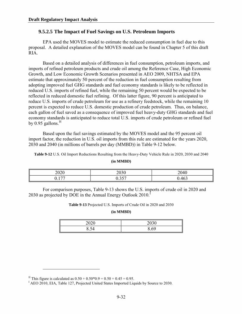
Draft Regulatory Impact Analysis
9-32
9.5.2.5 The Impact of Fuel Savings on U.S. Petroleum Imports
EPA used the MOVES model to estimate the reduced consumption in fuel due to this proposal. A detailed explanation of the MOVES model can be found in Chapter 5 of this draft RIA.
Based on a detailed analysis of differences in fuel consumption, petroleum imports, and imports of refined petroleum products and crude oil among the Reference Case, High Economic Growth, and Low Economic Growth Scenarios presented in AEO 2009, NHTSA and EPA estimate that approximately 50 percent of the reduction in fuel consumption resulting from adopting improved fuel GHG standards and fuel economy standards is likely to be reflected in reduced U.S. imports of refined fuel, while the remaining 50 percent would be expected to be reflected in reduced domestic fuel refining. Of this latter figure, 90 percent is anticipated to reduce U.S. imports of crude petroleum for use as a refinery feedstock, while the remaining 10 percent is expected to reduce U.S. domestic production of crude petroleum. Thus, on balance, each gallon of fuel saved as a consequence of improved fuel heavy-duty GHG standards and fuel economy standards is anticipated to reduce total U.S. imports of crude petroleum or refined fuel by 0.95 gallons.H
Based upon the fuel savings estimated by the MOVES model and the 95 percent oil import factor, the reduction in U.S. oil imports from this rule are estimated for the years 2020, 2030 and 2040 (in millions of barrels per day (MMBD)) in
Table 9-12 below.
Table 9-12 U.S. Oil Import Reductions Resulting from the Heavy-Duty Vehicle Rule in 2020, 2030 and 2040
(in MMBD)
2020 2030 2040 0.177 0.357 0.463
For comparison purposes, Table 9-13 shows the U.S. imports of crude oil in 2020 and 2030 as projected by DOE in the Annual Energy Outlook 2010.I
Table 9-13 Projected U.S. Imports of Crude Oil in 2020 and 2030
(in MMBD)
2020 2030 8.54 8.69
H This figure is calculated as 0.50 + 0.50*0.9 = 0.50 + 0.45 = 0.95. I AEO 2010, EIA, Table 127, Projected United States Imported Liquids by Source to 2030.

Chapter 9: Other Economic and Social Impacts
9-33
9.5.2.6 Energy Security Benefits of this Proposed Program
Using the same methodology as the peer reviewed model, but updating the analysis using AEO 2010 world oil price values and the estimated fuel savings from the rule using the MOVES model, EPA has calculated the energy security benefits of the rule for the years 2020, 2030 and 2040. Since the Agency is taking a global perspective with respect to valuing greenhouse gas benefits from the rule, only the macroeconomic adjustment/disruption portion of the energy security premium is used in the energy security benefits estimates present below. These results are shown below in Table 9-14.
Table 9-14 U.S. Energy Security Benefits of the Heavy-Duty Vehicle Rulemaking in 2020, 2030 and 2040
(in millions of $2008)
2020 2030 2040 $479 $1,117 $1,526
9.6 Summary of Benefits and Costs
In this section, the agencies present a summary of costs, benefits, and net benefits of the proposal. Table 9-15 shows the estimated annual monetized costs of the proposed program for the indicated calendar years. The table also shows the net present values of those costs for the calendar years 2012-2050 using both 3 percent and 7 percent discount rates.J
Table 9-15 Estimated Monetized Costs of the Proposed Program (Millions of 2008 dollars)
In this table, the aggregate value of fuel savings is calculated using pre-tax fuel prices since savings in fuel taxes do not represent a reduction in the value of economic resources utilized in producing and consuming fuel. Note that fuel savings shown here result from reductions in fleet-wide fuel use. Thus, they grow over time as an increasing fraction of the fleet meets the 2018 standards.
a
2020 2030 2040 2050 NPV, YEARS 2012-
2050, 3% DISCOUNT RATE
NPV, YEARS 2012-2050, 7% DISCOUNT
RATE Truck/Tractor Costs $2,000 $1,900 $2,200 $2,500 $42,100 $22,500
Fuel Savings (pre-tax)
-$8,100
-$19,000
-$28,100
-$35,400 -$352,300 -$152,600
Quantified Annual Costs
-$6,100
-$17,100
-$25,900
-$32,900 -$310,200 -$130,100
a Technology costs and fuel savings for separate truck segments can be found in Chapter 7.
Table 9-16 presents estimated annual monetized benefits for the indicated calendar years. The table also shows the net present values of those benefits for the calendar years 2012-2050
J For the estimation of the stream of costs and benefits, we assume that after implementation of the proposed MY 2014-2017 standards, the 2017 standards apply to each year out to 2050.

Draft Regulatory Impact Analysis
9-34
using both 3 percent and 7 percent discount rates. The table shows the benefits of reduced CO2
In addition, these monetized GHG benefits exclude the value of reductions in non-CO
emissions—and consequently the annual quantified benefits (i.e., total benefits)—for each of four SCC values estimated by the interagency working group. As discussed in Section 8.5, there are some limitations to the SCC analysis, including the incomplete way in which the integrated assessment models capture catastrophic and non-catastrophic impacts, their incomplete treatment of adaptation and technological change, uncertainty in the extrapolation of damages to high temperatures, and assumptions regarding risk aversion.
2 GHG emissions (CH4, N2O, HFC) expected under this proposal. Although EPA has not monetized the benefits of reductions in non-CO2 GHGs, the value of these reductions should not be interpreted as zero. Rather, the net reductions in non-CO2
Table 9-16 Monetized Benefits Associated with the Proposed Program (Millions of 2008 dollars)
GHGs will contribute to this rule’s climate benefits, as explained in Section III.F of the preamble.
2020 2030 2040 2050 NPV, YEARS 2012-2050, 3% DISCOUNT RATEA
NPV, YEARS 2012-2050, 3% DISCOUNT RATEA
Reduced CO2 Emissions at each assumed SCC valueb
5% (avg SCC) $200 $700 $1,200 $1,700 $8,600 $8,600 3% (avg SCC) $900 $2,300 $3,600 $4,900 $44,000 $44,000 2.5% (avg SCC) $1,500 $3,500 $5,300 $7,100 $74,600 $74,600 3% (95th percentile) $2,800 $7,100 $10,800 $14,800 $134,100 $134,100 Energy Security Impacts (price shock) $500 $1,100 $1,500 $1,800 $19,800 $8,700
Accidents, Noise, Congestion -$200 -$400 -$500 -$600 -$7,500 -$3,400
Refueling Savings $100 $100 $200 $200 $2,500 $1,100 Non-CO2
Non-GHG Impacts c,d
GHG Impacts and n/a n/a n/a n/a n/a n/a
Total Annual Benefits at each assumed SCC valueb
5% (avg SCC) $600 $1,500 $2,400 $3,100 $23,400 $15,000 3% (avg SCC) $1,300 $3,100 $4,800 $6,300 $58,800 $50,400 2.5% (avg SCC) $1,900 $4,300 $6,500 $8,500 $89,400 $81,000 3% (95th percentile) $3,200 $7,900 $12,000 $16,200 $148,900 $140,500
a Note that net present value of reduced CO2
b Section 8.5 of the RIA notes that SCC increases over time. Corresponding to the years in this table, the SCC estimates range as follows: for Average SCC at 5%: $5-$16; for Average SCC at 3%: $22-$46; for Average SCC at 2.5%: $36-$66; and for 95th percentile SCC at 3%: $66-$139. Section VIII.F also presents these SCC estimates.
emissions is calculated differently than other benefits. The same discount rate used to discount the value of damages from future emissions (SCC at 5, 3, 2.5 percent) is used to calculate net present value of SCC for internal consistency. Refer to the SCC TSD for more detail.
c The monetized GHG benefits presented in this analysis exclude the value of changes in non-CO2 GHG emissions expected under this proposal (see RIA Chapter 5). Although EPA has not monetized changes in non-CO2
d Non-GHG-related health and welfare impacts (related to PM
GHGs, the value of any increases or reductions should not be interpreted as zero.
2.5
and ozone exposure) were not estimated for this proposal, but will be included in the analysis of the final rulemaking.
Table 9-17 presents estimated annual net benefits for the indicated calendar years. The table also shows the net present values of those net benefits for the calendar years 2012-2050 using both 3 percent and 7 percent discount rates. The table includes the benefits of reduced

Chapter 9: Other Economic and Social Impacts
9-35
CO2
Table 9-17 Monetized Net Benefits Associated with the Proposed Program (Millions of 2008 dollars)
emissions (and consequently the annual net benefits) for each of four SCC values considered by EPA.
2020 2030 2040 2050 NPV, 3% NPV, 7% Annual Costsa -$6,100 -$17,100 -$25,900 -$32,900 -$310,200 -$130,100
Monetized Annual Benefits at each assumed SCC value 5% (avg SCC) $600 $1,500 $2,400 $3,100 $23,400 $15,000 3% (avg SCC) $1,300 $3,100 $4,800 $6,300 $58,800 $50,400 2.5% (avg SCC) $1,900 $4,300 $6,500 $8,500 $89,400 $81,000 3% (95th percentile) $3,200 $7,900 $12,000 $16,200 $148,900 $140,500
Monetized Net Benefits at each assumed SCC value 5% (avg SCC) $6,700 $18,600 $28,300 $36,000 $333,600 $145,100 3% (avg SCC) $7,400 $20,200 $30,700 $39,200 $369,000 $180,500 2.5% (avg SCC) $8,000 $21,400 $32,400 $41,400 $399,600 $211,100 3% (95th percentile) $9,300 $25,000 $37,900 $49,100 $459,100 $270,600
a Note that negative costs represent savings rather than costs.
EPA also conducted a separate analysis of the total benefits over the model year lifetimes of the 2014 through 2018 model year trucks/tractors. In contrast to the calendar year analysis presented in Table 9-15 through Table 9-17, the model year lifetime analysis shows the impacts of the proposed program on vehicles produced during each of the model years 2014 through 2018 over the course of their expected lifetimes. The net societal benefits over the full lifetimes of vehicles produced during each of the five model years from 2014 through 2018 are shown in Table 9-18 and Table 9-19 at both 3 percent and 7 percent discount rates, respectively.
Table 9-18 Monetized Costs, Benefits, and Net Benefits Associated with the Lifetimes of 2014-2018 Model Year Trucks (Millions of 2008 dollars; 3% Discount Rate)
2014MY 2015MY 2016MY 2017MY 2018MY SUM Monetized Costs
Technology Costs -$1,300 -$1,300 -$1,500 -$1,600 -$2,000 -$7,700 Monetized Benefits at each assumed SCC value
Pre-tax Fuel Savings $6,100 $6,400 $7,200 $10,700 $11,900 $42,300 Energy Security $400 $400 $400 $600 $700 $2,500 Accidents, Noise, Congestion -$300 -$300 -$300 -$300 -$300 -$1,400 Refueling Savings $200 $200 $200 $200 $200 $1,100 Non-CO2Non-GHG Impacts a,b
GHG Impacts and n/a n/a n/a n/a n/a n/a
Reduced CO2 emissions at each assumed SCC value 5% (avg SCC) $200 $200 $200 $300 $300 $1,200 3% (avg SCC) $600 $600 $700 $1,000 $1,200 $4,100 2.5% (avg SCC) $1,000 $1,000 $1,100 $1,600 $1,800 $6,500 3% (95th percentile) $1,900 $2,000 $2,200 $3,200 $3,500 $12,800
Monetized Net Benefits at each assumed SCC value 5% (avg SCC) $5,300 $5,600 $6,200 $9,900 $10,800 $38,000 3% (avg SCC) $5,700 $6,000 $6,700 $10,600 $11,700 $40,900 2.5% (avg SCC) $6,100 $6,400 $7,100 $11,200 $12,300 $43,300 3% (95th percentile) $7,000 $7,400 $8,200 $12,800 $14,000 $49,600

Draft Regulatory Impact Analysis
9-36
a The monetized GHG benefits presented in this analysis exclude the value of changes in non-CO2 GHG emissions expected under this proposal (see RIA Chapter 5). Although EPA has not monetized changes in non-CO2
b Non-GHG-related health and welfare impacts (related to PM
GHGs, the value of any increases or reductions should not be interpreted as zero.
2.5
and ozone exposure) were not estimated for this proposal, but will be included in the analysis of the final rulemaking.
Table 9-19 Monetized Costs, Benefits, and Net Benefits Associated with the Lifetimes of 2014-2018 Model Year Trucks (Millions of 2008 dollars; 7% Discount Rate)
2014MY 2015MY 2016MY 2017MY 2018MY SUM Monetized Costs
Technology Costs -$1,300 -$1,300 -$1,500 -$1,600 -$2,000 -$7,700 Monetized Benefits at each assumed SCC value
Pre-tax Fuel Savings $4,500 $4,500 $4,900 $7,000 $7,500 $28,400 Energy Security $300 $300 $300 $400 $400 $1,700 Accidents, Noise, Congestion -$200 -$200 -$200 -$200 -$200 -$900 Refueling Savings $200 $200 $200 $200 $200 $900 Non-CO2Non-GHG Impacts a,b
GHG Impacts and n/a n/a n/a n/a n/a n/a
Reduced CO2 emissions at each assumed SCC value 5% (avg SCC) $200 $200 $200 $300 $300 $1,200 3% (avg SCC) $600 $600 $700 $1,000 $1,200 $4,100 2.5% (avg SCC) $1,000 $1,000 $1,100 $1,600 $1,800 $6,500 3% (95th percentile) $1,900 $2,000 $2,200 $3,200 $3,500 $12,800
Monetized Net Benefits at each assumed SCC value 5% (avg SCC) $3,700 $3,700 $3,900 $6,100 $6,200 $23,600 3% (avg SCC) $4,100 $4,100 $4,400 $6,800 $7,100 $26,500 2.5% (avg SCC) $4,500 $4,500 $4,800 $7,400 $7,700 $28,900 3% (95th percentile) $5,400 $5,500 $5,900 $9,000 $9,400 $35,200
a The monetized GHG benefits presented in this analysis exclude the value of changes in non-CO2 GHG emissions expected under this proposal (see RIA Chapter 5). Although EPA has not monetized changes in non-CO2
b Non-GHG-related health and welfare impacts (related to PM
GHGs, the value of any increases or reductions should not be interpreted as zero.
2.5
and ozone exposure) were not estimated for this proposal, but will be included in the analysis of the final rulemaking.

Chapter 9: Other Economic and Social Impacts
9-37
Reference
1 Environmental Protection Agency and Department of Transportation, “Light-Duty Vehicle Greenhouse Gas Emissions Standards and Corporate Average Fuel Economy Standards; Final Rule,” Federal Register 75(88) (May 7, 2010). See especially sections III.H.1 (pp. 25510-25513) and IV.G.6 (pp. 25651-25657).
2 American Transportation Research Institute, An Analysis of the Operational Costs of Trucking, December 2008 (Docket ID: EPA-HQ-OAR-2010-0162-0007).
3 Transport Canada, Operating Cost of Trucks, 2005. See http://www.tc.gc.ca/eng/policy/report-acg-operatingcost2005-2005-e-2-1727.htm, accessed on July 16, 2010 (Docket ID: EPA-HQ-OAR-2010-0162-0006).
4 Graham and Glaister, “Road Traffic Demand Elasticity Estimates: A Review,” Transport Reviews Volume 24, 3, pp. 261-274, 2004 (Docket ID: EPA-HQ-OAR-2010-0162-0005).
5 Winston, C. (1981). The welfare effects of ICC rate regulation revisited. The Bell Journal of Economics, 12, 232-244 (Docket ID: EPA-HQ-OAR-2010-0162-0021).
6 Committee to Assess Fuel Economy Technologies for Medium- and Heavy-Duty Vehicles; National Research Council; Transportation Research Board (2010). Technologies and Approaches to Reducing the Fuel Consumption of Medium- and Heavy-Duty Vehicles. ("The NAS Report") Washington, D.C., The National Academies Press. Available electronically from the National Academy Press Website at http://www.nap.edu/catalog. See also 2009 Cambridge Systematics, Inc., Draft Final Paper commissioned by the NAS in support of the medium-duty and heavy-duty report. Assessment of Fuel Economy Technologies for Medium and Heavy Duty Vehicles: Commissioned Paper on Indirect Costs and Alternative Approaches (Docket ID: EPA-HQ-OAR-2010-0162-0009).
7 Friedlaender, A. and Spady, R. (1980) A derived demand function for freight transportation, Review of Economics and Statistics, 62, pp. 432–441 (Docket ID: EPA-HQ-OAR-2010-0162-0004).
8 Christidis and Leduc, “Longer and Heavier Vehicles for freight transport,” European Commission Joint Research Center’s Institute for Prospective Technology Studies, 2009 (Docket ID: EPA-HQ-OAR-2010-0162-0010).
9 Christidis and Leduc, 2009.
10 Winebrake, James and James J. Corbett (2010). “Improving the Energy Efficiency and Environmental Performance of Goods Movement,” in Sperling, Daniel and James S. Cannon (2010) Climate and Transportation Solutions: Findings from the 2009 Asilomar Conference on Transportation and Energy Policy. See http://www.its.ucdavis.edu/events/2009book/Chapter13.pdf (Docket ID: EPA-HQ-OAR-2010-0162-0011)
11 Winebrake, J. J.; Corbett, J. J.; Falzarano, A.; Hawker, J. S.; Korfmacher, K.; Ketha, S.; Zilora, S., Assessing Energy, Environmental, and Economic Tradeoffs in Intermodal Freight Transportation, Journal of the Air & Waste Management Association, 58(8), 2008 (Docket ID: EPA-HQ-OAR-2010-0162-0008).
12 Cambridge Systematics, Inc.. 2009.
13 Northeast States Center for a Clean Air Future, Southeast Research Institute, TIAX, LLC., and International Council on Clean Transportation, Reducing Heavy-Duty Long Haul Truck Fuel Consumption and CO2 Emissions, September 2009. See http://www.nescaum.org/documents/heavy-duty-truck-ghg_report_final-200910.pdf
14 These estimates were developed by FHWA for use in its 1997 Federal Highway Cost Allocation Study; see http://www.fhwa.dot.gov/policy/hcas/final/index.htm (last accessed July 21, 2010).

Draft Regulatory Impact Analysis
9-38
15 See Federal Highway Administration, 1997 Federal Highway Cost Allocation Study, http://www.fhwa.dot.gov/policy/hcas/final/index.htm, Tables V-22, V-23, and V-24 (last accessed July 21, 2010).
16 See Table 4. Last viewed on September 9, 2010 at http://ostpxweb.dot.gov/policy/Data/VOTrevision1_2-11-03.pdf. Note that we assume the value of travel time is constant out to 2050, which is a conservative assumption since it is likely this value will increase due to income growth in the future.
17 Passenger vehicle fuel dispensing rate per EPA regulations, last viewed on August 4, 2010 at http://www.epa.gov/oms/regs/ld-hwy/evap/spitback.txt 18 U.S. Bureau of Economic Analysis, U.S. International Transactions Accounts Data, as shown on June 14, 2010. 19 U.S. Department of Energy, Annual Energy Review 2008, Report No. DOE/EIA-0384(2008), Tables 5.1 and 5.13c, June 26, 2009. 20 Leiby, Paul N. "Estimating the Energy Security Benefits of Reduced U.S. Oil Imports," Oak Ridge National Laboratory, ORNL/TM-2007/028, Final Report, 2008.
21 Leiby, Paul N., Donald W. Jones, T. Randall Curlee, and Russell Lee, Oil Imports: An Assessment of Benefits and Costs, ORNL-6851, Oak Ridge National Laboratory, November, 1997.
22 Peer Review Report Summary: Estimating the Energy Security Benefits of Reduced U.S. Oil Imports, ICF, Inc., September 2007. 23 Gately, Dermot 2004. "OPEC's Incentives for Faster Output Growth," The Energy Journal, 25(2):75-96, "What Oil Export Levels Should We Expect From OPEC?" The Energy Journal, 28(2):151-173, 2007

Heavy-Duty GHG and Fuel Efficiency Standards NPRM: Small Business Flexibility Analysis
10-1
CHAPTER 10: Small Business Flexibility Analysis The Regulatory Flexibility Act, as amended by the Small Business Regulatory
Enforcement Fairness Act of 1996 (SBREFA), generally requires an agency to prepare a regulatory flexibility analysis for any rule subject to notice-and-comment rulemaking requirements under the Administrative Procedure Act or any other statute. This requirement does not apply if the agency certifies that the rule will not have a significant economic impact on a substantial number of small entities.
The following discussion provides an overview of small entities in the heavy-duty vehicle and engine market. Small entities include small businesses, small organizations, and small governmental jurisdictions. For the purposes of assessing the impacts of the rule on small entities, a small entity is defined as: (1) a small business that meets the definition for business based on the Small Business Administration’s (SBA) size standards (see Table 10-1); (2) a small governmental jurisdiction that is a government of a city, county, town, school district or special district with a population of less than 50,000; and (3) a small organization that is any not-for-profit enterprise which is independently owned and operated and is not dominant in its field. Table 10-1 provides an overview of the primary SBA small business categories potentially affected by this regulation.
Table 10-1 Primary Small Business NAICS Categories Affected by this Rulemaking
NAICS CODES1 DEFINED BY SBA AS A SMALL BUSINESS IF LESS THAN OR EQUAL TO:
2
Engine Equipment Manufacturer
333618 1,000 employees Automobile Manufacturer 336111 1,000 employees Light Truck and Utility Vehicle Manufacturer
336112 1,000 employees
Heavy-Duty Truck Manufacturer 336120 1,000 employees Motor Vehicle Body Manufacturing 336211 1,000 employees
We compiled a list of engine manufacturers, vehicle manufacturers, and body manufacturers that would be potentially affected by the rule from the EPA database for engine certification, Ward’s Automotive Database, and the M.J. Bradley’s Heavy Duty Vehicle Market Analysis. We then identified companies that appear to meet the definition of small business provided in the table above based on the number of employees based on company information included in Hoover’s. Based on this assessment, the agencies identified the following:
• two tractor manufacturers3 which comprise less than 0.5 percent of the total heavy-duty combination tractors in the U.S. based on Polk Registration Data from 2003 through 2007;4

Regulatory Impact Analysis
10-2
• ten chassis manufacturers5 less than 0.5 percent of the total heavy-duty combination tractors in the U.S. based on Polk Registration Data from 2003 through 2007;6
• three heavy duty engine manufacturers
and
7
The proposed exemption from the standards established under this proposal would have a negligible impact on the GHG emissions and fuel consumption reductions otherwise due to the standards.
which comprise less than 0.1 percent of total heavy-duty engine based on 2008 and 2009 model year engine certification data submitted to EPA for non-GHG emissions standards.
EPA has not conducted an Initial Regulatory Flexibility Analysis for this proposed rulemaking because we are certifying that the rule would not have a significant economic impact on a substantial number of small entities. EPA is exempting manufacturers, domestic and foreign, meeting SBA’s size definitions of small business as described in 13 CFR § 121.201. EPA will instead consider appropriate GHG standards for these entities as part of a future regulatory action.
To ensure that EPA and NHTSA are aware of which companies would be exempt, the agencies propose to require that such entities submit a declaration to EPA containing a detailed written description of how that manufacturer qualifies as a small entity under the provisions of 13 CFR § 121.201.

Heavy-Duty GHG and Fuel Efficiency Standards NPRM: Small Business Flexibility Analysis
10-3
References
1 North American Industry Classification System 2 According to SBA’s regulations (13 CFR Part 121), businesses with no more than the listed number of employees or dollars in annual receipts are considered “small entities” for RFA purposes. 3 The agencies have identified Ottawa Truck, Inc. and Kalmar Industries USA as two potential small tractor manufacturers 4 M.J. Bradley. Heavy Duty Vehicle Market Analysis. May 2009. 5 The agencies have identified Lodal, Indiana Phoenix, Autocar LLC, HME, Giradin, Azure Dynamics, DesignLine International, Ebus, Krystal Koach, and Millenium Transit Services LLC as potential small business chassis manufacturers. 6 M.J. Bradley. Heavy Duty Vehicle Market Analysis. May 2009. 7 The agencies have identified Baytech Corporation, Clean Fuels USA, and BAF Technologies, Inc. as three potential small businesses