DRAFT — EURASIP JWCN 1 Correlation-based Radio...

DRAFT — EURASIP JWCN 1

Correlation-based Radio Localization

in an Indoor Environment

Thomas Callaghan, Nicolai Czink, Francesco Mani, Arogyaswami Paulraj,

George Papanicolaou

Abstract

We investigate the feasibility of using correlation-basedmethods for estimating the spatial location

of distributed receiving nodes in an indoor environment. Our algorithms do not assume any knowledge

regarding the transmitter locations or the transmitted signal, but do assume that there are ambient signal

sources whose location and properties are, however, not known.

The key idea is to compute pairwise cross correlations of thesignals received at the nodes and

use them to estimate the travel time between these nodes. If the ambient signal sources have sufficient

space-time diversity, then the cross correlations recoverthe distance between the two receiving nodes.

By doing this for all pairs of receivers we can construct an approximate map of their location using

multidimensional scaling methods.

We test this localization algorithm in a cubicle-style office environment based on both ray-tracing

simulations, and measurement data from a radio measurementcampaign using the Stanford broadband

channel sounder. Contrary to what is seen in other applications of cross-correlation methods, the strongly

scattering nature of the indoor environment complicates distance estimation. However, using statistical

methods, the rich multipath environment can be turned partially into an advantage by enhancing ambient

signal diversity and therefore making distance estimationmore robust.

The main result is that with our correlation-based statistical estimation procedure applied to the real

data, assisted by multidimensional scaling, we were able tocompute spatial antenna locations with an

average error of about 2 meters and pairwise distance estimates with an average error of 2.33 meters.

The theoretical resolution limit for the distance estimates is 1.25 meters.

Part of this work was supported by US Army grant W911NF-07-2-0027-1, by AFOSR grant FA9550-08-1-0089, by the

Austria Science Fund (FWF) through grant NFN SISE (S10607).FTW is supported by the Austrian Government and by the

City of Vienna within the competence center program COMET.

December 2, 2010 DRAFT


Index Terms

indoor localization; sensor networks; signal correlations; rich scattering; multidimensional scaling

I. INTRODUCTION

Indoor localization is a long-standing open problem in wireless communications [1], partic-

ularly in wireless sensor networks [2], [3]. Localization techniques in non-line-of-sight indoor

environments face two major challenges: (i) multipath fromrich scattering makes it difficult

to identify the direct path, limiting thus the use of distance estimation based on time-delay-of-

arrival (TDOA) methods; (ii) the strongly changing propagation loss due to shadowing impairs

distance estimation based on the received signal strength (RSS).

In both kinds of algorithms, TDOA and RSS, nodes can estimatetheir own location relative to

several “anchor nodes” acting as transmitters. This is commonly done by estimating the distances

to the anchor nodes and subsequently using triangularization for position estimation.

The estimation of the TDOA is done either by round-trip time estimation [4], the transmission

of specific training sequences [5], or simply by detecting the first peak of the received signal [6].

Ultra-wide band communications are specifically suited forTDOA distance estimation because

of the large available bandwidth [7].

Many publications discuss RSS-based distance estimation.The work presented in [8] provides

a comprehensive overview of an actual implementation usingWiFi hotspots in a self-configuring

network.

Another technique described in [9] is using spatial signatures for localization. However, this

requires multiple antennas at the nodes and a database of spatial locations. Moreover, this

technique is bound to specific antenna requirements.

Correlation-based methods [10] have been widely used for many years in a variety of fields,

including sensor networks. Some examples include estimation of the speed of seismic waves and

even earth-quake prediction [11]. The idea there is to crosscorrelate seismic noise signals from

sensors deployed in a wide area so as to estimate the travel time of the seismic waves from one

sensor to the other. Given the sensor locations, the wave speed can be estimated using travel

time tomography.

Contribution We investigate here the feasibility ofpassive, correlation-based indoor radio

localization. In contrast to the previous works, we consider both the source positions and the



source signals to be unknown. We just require that there are ambient signals present. The

receiving nodes estimate their distances to other nodes in athree step procedure: (i) first, all nodes

are receiving and storing ambient signals, (ii) the nodes communicate their received signals to

other nodes, (iii) the nodes estimate the pairwise distances between them by cross correlating their

received signals and identifying peaks in the cross-correlation function. If the ambient signals

have sufficient spatial diversity, then the peaks of the cross correlations provide a robust estimate

of the distance between the two receiving antennas. By doingthis for all pairs of receiving nodes,

we construct an approximate map of their locations using weighted least squares methods, in

particular multidimensional scaling (MDS) [12], [13].

We quantify the performance of the algorithms in an indoor environment with both ray-

tracing simulations and data from a recently conducted radio measurement campaign, using the

RUSK Stanford multi-antenna radio channel sounder with a center frequency of 2.45 GHz and

bandwidth of 240 MHz [14].

The strongly scattering nature of the indoor environment makes the pairwise distance es-

timation challenging. However, in contrast to other localization methods, multipath from rich

scattering is now both helpful and harmful for distance estimation. While multipath increases

spatial diversity, it also leads to additional peaks in the correlation function. The main feature

in this work is the proper treatment and utilization of the beneficial properties of rich multipath

while controlling its negative effects. To achieve this goal, we propose statistical peak-selection

algorithms that significantly increases the localization accuracy.

We demonstrate, therefore, that passive, correlation-based radio localization is feasible in

wireless indoor environments.

Organization The paper is organized as follows. Section II provides a brief motivation for

using correlation-based methods for distance estimation.In Section III we consider the problem

of travel time estimation using cross correlations. Section IV presents different approaches

for improving the pairwise travel-time estimation based oncorrelation-based methods. Section

V briefly presents how we use MDS to find position estimates, discusses the results from

applying our algorithms and MDS to the simulated and measured data, and demonstrates the

effect of transmitter positions using the simulated data. With Section VII we conclude the

paper. Appendices A and B provide brief descriptions of the ray-tracing simulations and the

measurement data we use in this paper.



II. M OTIVATION FOR THE USE OFCROSSCORRELATIONS IN DISTANCE ESTIMATION

We start out with a simple example. Consider a line-of-sightenvironment, as shown in Figure 1.

A single source emits a pulses(τ) = δ(τ), while two receivers record the signalsr1(τ) andr2(τ),

respectively, whereτ denotes the delay andδ(·) denotes the Dirac delta function. The positions

of the source and of the receivers are unknown. The signal emitted by the source is received by

both receivers with certain delay lags. Thus, the received signals becomer1(τ) = γ1δ(τ − τ1),

and r2(τ) = γ2δ(τ − τ2), whereτk denotes the delay lag from the source to thekth receiver,

andγk denotes the path loss of the signal. By cross correlating thetwo received signals,

c1,2(τ) =

∫

r1(τ′)r2(τ + τ ′)dτ ′ = γ1γ2δ(τ − (τ1 − τ2)), (1)

we see that the resulting cross correlation is a pulse at the delay difference∆τ = τ1 − τ2. This

also holds for arbitrary source signals, as long as they havecertain auto-correlation properties,

as shown in the next section.

By finding the peak in the received signals cross correlation, we can estimate the distance

between the receivers asd = ∆τ c0, with c0 indicating the speed of light. When the transmitter

is on a straight line going through the two receivers, this estimated distance is the exact distance

between the nodes [10]. However, when there is an angleα between the direction of the plane

wave front and the straight line between the receivers, the distance estimate will gived =

d | cos(α)|, which carries a systematic error.

Since we do not know the position of the source, we cannot correct for this systematic

error, but we can quantify its distribution. For this we makethe following assumptions: (i)

we consider horizontal wave propagation only, since it is predominant in indoor environments;

(ii) all directions of the transmitted signals are equally likely, i.e. α is distributed uniformly,

α ∼ U [−π, π). So, we can calculate the probability density function of the estimated distance,

pd(d) by transformation of the random variableα as

pd(d) =

2π

1

d√

1−(d/d)2. . . 0 ≤ d ≤ d,

0 . . . d > d,(2)

and also obtain its cumulative distribution function

F (d) =2

πarcsin

(

d

d

)

. . . 0 ≤ d ≤ d, (3)



which is shown in Figure 2. It turns out that in 50% of all cases, our distance estimation error

is less than 30% (indicated by the dashed lines).

While basing the distance estimation on a single plane wave is questionable because of the

rather large systematic error, real radio propagation environments provide diversity by multiple

sources and by multipath. The receiver cross correlation will therefore have multiple peaks,

which provide more information about the propagation environment, which improves distance

estimation. The way to exploit this signal diversity and howto obtain a robust distance estimate

is the topic of the rest of this paper.

To provide another motivation as to why cross correlations can be used for travel time

estimation, we’ll briefly review results for cross correlations in a homogeneous environment

[10], [15], [16]. Let r1(t) and r2(t) denote the time-dependent wave fields recorded by two

sensors atx1 andx2. Their cross correlation function over the time interval[0, T ] with time lag

τ is given by

c1,2(τ) =1

T

∫ T

0

r1(t)r2(t+ τ)dt

In the case of a 3-D homogeneous medium with spatially uniform noise source distribution, the

field at each receiver can be decomposed as a superposition ofuncorrelated plane waves from

various directions. It has been established that the normalized cross-spectral densityc1,2(ω) at

frequencyω between two sensorsx1 andx2 separated byr is c1,2(ω) = [sin(ωr/c)]/(ωr/c). In

the time domain, the normalized correlation function is

c1,2(τ) =1

2π

∫ ∞

−∞

c1,2(ω)ejωτdω

=1

4π

∫ ∞

−∞

[

ejω(τ+r/c)

jωr/c− ejω(τ−r/c)

jωr/c

]

dω

The time derivative of the cross correlation function is

d

dτc1,2(τ) =

1

4πr/c[δ(τ + r/c)− δ(τ − r/c)] .

These two terms correspond to the forward and backward (symmetrized in time)impulse response

function between the two receivers. From the peaks of these functions, one can deduce the travel

time between sensorsx1 andx2. This result has been shown to extend to scattering media as

well [10], where the delta functions on the right are replaced by the time dependent Green’s

function (channel transfer function) between the two receivers.



Based on this motivation, the theory indicates that the peakof the derivative of the cross

correlation function is a good estimate of the travel time. However, due to the strongly scat-

tering medium, the cross correlation is not smooth and has many peaks making the derivative

computation unreliable. Instead we use the other motivation and use the peaks from the cross

correlation function to estimate the travel time (and distance).

III. COMPUTATION OF CROSSCORRELATIONS

This section describes the computation of the cross correlations using a more complex setting

with multiple sources, including scattering in the environment. A finite number ofL sources,

Sl, l = 1 . . . L, transmit random uncorrelated signalssl(t, τ), i.e.

E {sl(t, τ)sl′(t′, τ ′)} =

1 . . . l = l′ ∧ τ = τ ′

0 . . . l 6= l′ ∨ τ 6= τ ′,

wheret denotes absolute time (assuming block transmission), andτ denotes the delay lag. For

example, white noise signals fulfill these properties asymptotically, whenτ → ∞. We assume

that the channel stays constant within the transmission of ablock and then changes due to fading.

A number ofK receivers,Rk, k = 1 . . .K, records their respective received signalsrk(t, τ) from

these multiple random sources, i.e.

rk(t, τ) =L∑

l=1

∫

τ ′sl(t, τ

′)hkl(t, τ − τ ′)dτ ′, (4)

wherehkl(t, τ) denotes the time and frequency selective radio channel fromthe lth source to

the kth receiver.

The cross correlation function (CCF) between two received signals at timet is

ck,k′(t, τ) =

∫

τ ′rk(t, τ

′)rk′(t, τ + τ ′)dτ ′, (5)

which can be written as

ck,k′(t, τ) =L∑

l=1

∫

τ ′hkl(t, τ

′)hk′l(t, τ + τ ′)dτ ′, (6)

when the source signals fulfill the condition in (4). This CCFprovides information about the

delay lag between the two receiversRk andRk′ as discussed in the previous section.



When applying this method to radio channel measurements, the CCF can be averaged over

all measured time instantsT (i.e. averaging over fading variations of the channel) by

ck,k′(τ) =1

T

T∑

t=1

ck,k′(t, τ). (7)

For the actual implementation, all convolutions and correlations in delay domain are imple-

mented as multiplications in frequency domain.

It is well known [10] that for an infinite number of (uncorrelated) orthogonal sources, spatially

distributed uniformly over all solid angles in 3-D, the resulting CCF has a rectangular shape,

centered at zero and having a width of2d/c0. Since in our simultaions and measurements

(cf. Appendices A and B) only a finite number of transmitting antennas contribute to the

signal recorded at each receiving antenna, we rely on sufficient scattering in the medium for

enhancement of directional diversity. This leads to a trade-off between two effects: (i) Multipath

increases the signal diversity and thus creates peaks in theCCF that better represent the true

distance, but (ii) multipath also generates ”wrong” (additional) peaks from propagation paths

that do not directly travel through the receivers, which in turn reduce the accuracy of distance

estimation.

An example of a CCF evaluated from our measurements (cf. Appendix B) is shown in Figure 3.

We observed a strong directionality of the impinging radio waves, which leads to peaks at various

distances. The true distance of4.9m, indicated by the dashed lines, is clearly visible as a peakin

the CCF. However, other strong peaks are also present. Because of these multiple peaks, which

sometimes dwarf the accurate peaks, a more elaborate distance estimation method is necessary.

IV. I MPROVED DISTANCE ESTIMATION METHOD

The distance estimation can be improved in by combining three ideas: (i) using short-time

estimates of the CCF, (ii) using multiple peaks from the CCF for distance estimation, and (iii)

using relative weighting on the peaks from the CCF to distinguish between peaks of comparable

height (power).

A. Short-time estimates of the CCF

The long-time averaging applied in the original approach in(7) may reduce information about

the propagation environment. By using the short-time estimates of the CCF from (5), individual



differences in the propagation environment, caused by fading, can be utilized to improve the

distance estimation as follows.

B. Multiple peaks for distance estimation

As motivated in Section II, the distance between two receivers is proportional to the propa-

gation delay,

dk,k′ = τk,k′ c0, (8)

wheredk,k′ and τk,k′ denote the distance estimate and travel time estimate, respectively.

A direct way to estimate the delay between two receivers is toidentify the largest peak in

their CCF. This approach does not perform well in multipath environments. Instead, we consider

a more robust statistical approach based onmultiple peaks in the CCF. The problem is how to

choose and how to use the peaks in the CCF.

We use a statistical approach as follows: the CCF is sorted according to

ck,k′(t, τ1) > ck,k′(t, τ2) > · · · > ck,k′(t, τM), (9)

with M denoting the number of resolved delays in the CCF. From this sorting, we usep = 0.5%

of the delays having the strongest CCF values, i.e.

τk,k′(t, n) = |τn|, n ∈ [1, . . . , ⌊pM⌋], (10)

which corresponds to taking the top 4 peaks in our data set.

We then take a weighted average of these multiple delays as the distance estimate, i.e.

τk,k′ =1

T · ⌊pM⌋

T∑

t=1

⌊pM⌋∑

n=1

wk,k′(t, n)τk,k′(t, n), (11)

where the choice of the weightswk,k′(t, n) is described in the next section.

C. Cross-Correlations with weights

To improve the distance estimation further, we propose to distinguish between dominant peaks

and peaks of similar amplitude. For this reason, we weigh thepeaks based on their relative

amplitude.



Since we are usingN = ⌊pM⌋ peaks, we assigned a weight to each peak equal to the ratio

between its amplitude over theN th largest peak’s amplitude,

wk,k′(t, n) = ck,k′(t, τn)/ck,k′(t, τN ), n ∈ [1, N ]. (12)

The estimates computed by this statistical procedure can subsequently be improved by taking

geometrical considerations into account as shown in the next section.

V. RESULTS

In the subsections that follow, we apply these distance estimation methods to both a simulated

dataset and data from an indoor radio channel measurement campaign. In addition to distance

estimation results, we also present localization results as estimated receiver positions are also of

much interest in this problem. To estimate positions from pairwise distance estimates between

all receivers, it is natural to use multidimensional scaling (MDS) algorithms. These statistical

techniques, that date back 50 years, take as its input a set ofpairwise similarities and assign

them locations in space [12], [13]. Recently, it was appliedto a different, but related problem,

of node localization in sensor networks [3].

In MDS we solve the following least-squares optimization problem

min{Rk}

∑

k 6=k′

λk,k′

∣

∣

∣dk,k′ − ||Rk − Rk′||2

∣

∣

∣

2

, (13)

wheredk,k′ are the provided distance estimates,λk,k′ are weights,|| · ||2 is the Euclidean distance,

and{Rk} is the set of locations of the receivers{Rk}. In our problem we assume the locations

to lie in R2. As we will show in the next section, the error in our pairwisedistance estimates is

correlated to the distance estimates themselves. Thus, a natural weighting isλk,k′ = 1/dαk,k′, for

α ≥ 0. We found thatα = 1 produced the smallest error. To solve this optimization problem,

we used the algorithm given in [17], which resulted in the final position estimates{Rk} of the

receivers. The results from solving this optimization problem are sensitive to the initial guess,

so we used the procedure to compute our initial position estimate in [18].

A. Ray-tracing simulations

We first present our localization method applied to a environment simulated using a state-

of-the-art ray-tracing tool including diffuse scattering. A detailed description of the ray tracing



algorithm is provided in Appendix A. The nodes were set up as shown in Figure 4. Weestimated

the distance between all pairs of nodes and calculated the distance estimation error using the

(“statistical peak selection”) method presented in Section IV. As reference to with which to

compare we use the long-time average peak method (“cumulative peak”), i.e. selecting the

strongest peak out of the averaged long-time CCF given in (7).

A scatter plot of the true distance versus the estimated distance for these approaches is shown

in Figure 5. This plot exhibits a significant underestimation bias. We expect this from the theory,

especially when we have strong sources illuminating from the “wrong” angle.

The empirical cdfs of the distance estimation errors are shown by the dashed lines in Figure 6.

Using only the peak of the averaged long-time CCF performs worst, by far, because it does not

use the diversity in time. In contrast, using our statistical peak selections, significantly lowers

the distance estimation error.

With the simulated channel bandwidth of 240 MHz, our theoretical resolution is limited to

an accuracy ofc/B = 1.25 meters. Our final results produced an average pairwise distance

estimation error of 4.55 meters.

Next, we used MDS to obtain position estimates. By the weights introduced in the MDS1,

we make use of the correlation between the distance estimation and its error. In Figure 7, the

localization results using our statistical method are shown. The true locations are denoted by

circles, while the estimated locations are marked by squares. The arrows are connecting the

estimates to their respective true locations.

Looking at this figure, we notice that the error is mostly in the x-direction. The reason for this

is the strong directionality of the waves coming mostly fromtop/bottom, but not from left/right.

This naturally leads to an underestimation of the distance between the horizontally-spaced node

pairs. We also observe that the receiving antennas that are lying centrally have the smallest

position estimation errors. This is due to the increased diversity of the source signals. We find

an average position estimation error of 3.66 m, with a minimum error of 1.25 m, a maximum

error of 5.87 m, and a standard deviation of 1.56 m.

Looking at the position estimates when using only the long-time average peak in Figure 8,

the results seem questionable. Some distances are stronglyunderestimated as already seen

1These weights are not to be confused with the weighting of thepeaks



in Figure 5. In this approach, reliable position estimationbecomes impossible. This clearly

demonstrates that multipath must not be ignored, but needs to be utilized to enable acceptable

distance estimation.

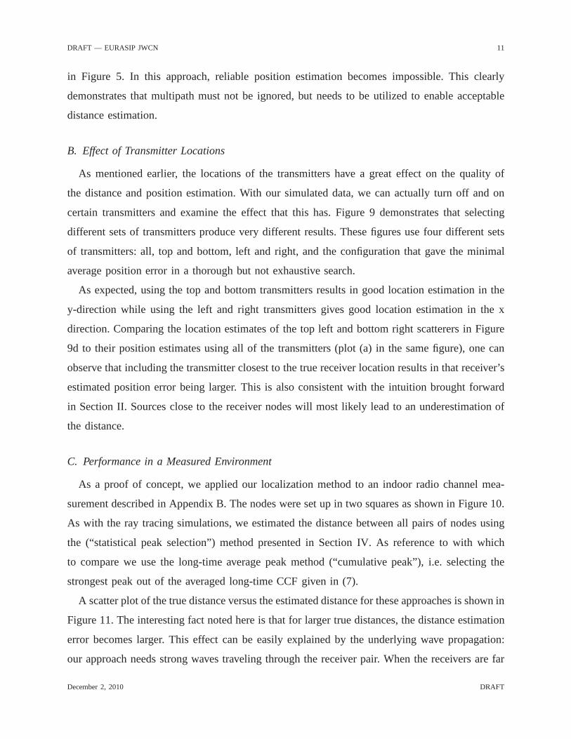
B. Effect of Transmitter Locations

As mentioned earlier, the locations of the transmitters have a great effect on the quality of

the distance and position estimation. With our simulated data, we can actually turn off and on

certain transmitters and examine the effect that this has. Figure 9 demonstrates that selecting

different sets of transmitters produce very different results. These figures use four different sets

of transmitters: all, top and bottom, left and right, and theconfiguration that gave the minimal

average position error in a thorough but not exhaustive search.

As expected, using the top and bottom transmitters results in good location estimation in the

y-direction while using the left and right transmitters gives good location estimation in the x

direction. Comparing the location estimates of the top leftand bottom right scatterers in Figure

9d to their position estimates using all of the transmitters(plot (a) in the same figure), one can

observe that including the transmitter closest to the true receiver location results in that receiver’s

estimated position error being larger. This is also consistent with the intuition brought forward

in Section II. Sources close to the receiver nodes will most likely lead to an underestimation of

the distance.

C. Performance in a Measured Environment

As a proof of concept, we applied our localization method to an indoor radio channel mea-

surement described in Appendix B. The nodes were set up in twosquares as shown in Figure 10.

As with the ray tracing simulations, we estimated the distance between all pairs of nodes using

the (“statistical peak selection”) method presented in Section IV. As reference to with which

to compare we use the long-time average peak method (“cumulative peak”), i.e. selecting the

strongest peak out of the averaged long-time CCF given in (7).

A scatter plot of the true distance versus the estimated distance for these approaches is shown in

Figure 11. The interesting fact noted here is that for largertrue distances, the distance estimation

error becomes larger. This effect can be easily explained bythe underlying wave propagation:

our approach needs strong waves traveling through the receiver pair. When the receivers are far



apart, the probability of a direct wave from one to the other becomes much lower. This is also

the reason why the long-time average peak method performs sobadly. The distance between the

nodes is strongly underestimated. Only when making use of fading, i.e. diversity in time, the

distance estimates become reliable. It is important to notethat this result is significantly different

than the result with the simulated data. This is due to the fact that the real measurements capture

more of the complexity of the rich scattering channel.

Again, the empirical cdfs of the distance estimation errorsare shown by the dashed lines in

Figure 12. With the measurement bandwidth of 240 MHz, our theoretical resolution is limited

to an accuracy ofc/B = 1.25 meters. Our final results produced an average pairwise distance

estimation error of 2.33 meters. Moreover, the distance estimation errors of almost half of our

28 receiving antenna pairs were below the resolution limit,which is again an effect of using the

diversity offered by the time variations in the channel.

We also present the results of thelocation estimation in Figure 13. The true locations are de-

noted by circles, while the estimated locations are marked by squares. The arrows are connecting

the estimates to their respective true locations.

Looking at the quadrangle of the bottom four nodes, we observe that the estimates are placed

in a rhomboid. The reason for this is the strong directionality of the waves coming mostly from

left/right, but not from top/bottom. This naturally leads to an underestimation of the distance

between the vertically-spaced node pairs. The result is that the nodes appear squeezed in the

y-direction, but do have the correct distance in the x-direction. We also observe that the receiving

antennas that are lying centrally have the smallest position estimation errors. This is due to the

increased diversity of the source signals. We find an averageposition estimation error of 2.1 m,

with a minimum error of 0.4 m, a maximum error of 3.36 m, and a standard deviation of 0.92 m.

The results are similar when using the multi-peak mean method without peak weighting.

As before, when using only the long-time average peak in Figure 14, the results are inaccurate

and unreasonable.

VI. I MPLEMENTATION

A realistic implementation of these methods would of courserequire the consideration of

several practical issues, including timing synchronization and information exchange between the



receiver nodes, and optimal selection of the radio band for providing enough ambient signal

strength.

Many of these issues can be resolved if we assume that we have amaster node with which all

receiver nodes can communicate so as to transfer their recorded data. Finally, the master node

performs all the calculations, and also ensures the synchronization between the nodes [19].

As for all delay-based localization algorithms, the receiving nodes need to sample the ambient

signals with a high sampling rate (and thus bandwidth) usinga fast analog-to-digital converter.

The advantage of our approach is that the sampling can be donewith a low bit resolution, against

which our approach is quite robust. Of course, the recorded data can be further compressed before

sending it on to the master. Thus, only a limited amount of data needs to be transmitted, leading

to a much smaller necessary bandwidth than what was needed for sampling the signal.

VII. CONCLUSIONS

In this paper we consider the feasibility of radio localization in a rich-scattering indoor

environment using correlation-based techniques.

We presented a systematic way to use peaks in the cross correlations of the received signals

for computing pairwise distance estimates and spatial location estimates for a passive network

of wireless receiving nodes (sensors). The robustness of the estimation is enhanced by multipath

due to scattering but its accuracy is diminished by it. The increased signal diversity improves the

estimation robustness, while generating many peaks in the cross correlations. To enhance inter

receiver (sensor) distance estimation, we consider utilize statistical methods that utilize multipath

effects by taking into account multiple fading realizations of the channel.

We demonstrated the feasibility of our approach using both simulated and real measurements in

a cubicle-style office environment. In our simulations, we use a 3-D ray-tracing tool, operating at

2.45 GHz, to measure the radio channels between 14 transmitters and 14 receivers in a simulated

cubical office environment with diffuse scattering. In the real measurements, the radio channels

between eight transmitters and eight receivers were measured using the RUSK Stanford channel

sounder, operating at 2.45 GHz with a bandwidth of 240 MHz. The experimental equipment

is special and favors our localization approach. Realisticimplementation would require several

practical aspects to be considered. Most importantly, a master node would be necessary to



centralize the computation and synchronize the receiver nodes. However, using our equipment,

we have demonstrated the feasibility of correlation-basedradio localization techniques.

Despite the lack of a large number of transmitting antennas,we were able utilize the spatial

diversity of the strongly scattering room by using our improved estimation methods. The main

result is that with the real data we were able to estimate spatial antenna locations with less than

2 meters error when the theoretical resolution limit is 1.25meters.

APPENDIX

A. Ray-tracing Simulations

Ray-Tracing (RT) is a site-specific geometrical technique that evaluates propagation paths

followed by rays as they interact with the environment. A keyfeature of indoor propagation

channels is diffuse scattering. For this reason, a classic 3-D RT tool [20], improved with

penetration and diffuse scattering [21], has been used in this work to model the channel. The

model of diffuse scattering is described in [22]. A geometrical description of the environment,

frequency, number of interactions and dielectric properties of materials are some of the input

parameters of a RT tool. In the following sections the ones used in this work are presented.

1) Setup Parameters: The simulation frequency has been set to 2.45 GHz. Antenna radiation

patterns are the ones of vertically polarized dipoles both at receive (Rx) and source/transmit

(Tx) side. Whenever Tx are placed at walls, they radiate onlyinto the relative half-space. A

maximum of three reflections, single diffraction and single-bounce scattering has been used in

the simulations. A directive scattering pattern model withscattering coefficientS = 0.4 and

beamwidthαr = 4 has been chosen. These paths were filtered using a rectangular filter in

frequency domain with a bandwidth of 240 MHz to resemble the measurements.

2) Simulated Environment: A cubicle-style office scenario has been used as input for theRT

tool. The dimensions of the room have been set to 50 m× 20 m with a height of 4 m. The

walls, the ceiling and the floor are supposed to be made of concrete. Cubicles are 4 m× 3 m

× 1.8 m, and are organized in two rows. Cubicles are represented by their metallic frames that

have been treated as perfect electric conductors. A number of 14 receiving nodes were placed in

these cubicles, while the ambient noise signals are generated by 14 sources placed at the outer

wall of the room. At both sides the antennas are placed at an height of 1 m. Fig. 4 shows a

2-D map of the simulated environment as well as the positionsof the receivers and sources. A



rough model for the human body as a rectangular parallelepiped has been used. For the human

body a classic two-thirds muscle homogeneous model [23], [24] has been used to get realistic

values. The time variance of the channel has been modeled by randomly placing ten persons in

the scenario in 100 different realizations. The relative dielectric permittivityεr was set to 9 for

concrete walls, and 35.2 for the human body, while the conductivity σ was set to 0.06 and 1.16,

respectively.

B. Radio Channel Measurements

In this paper we use channel measurements obtained during the Stanford July 2008 Radio

Channel Measurement Campaign. More details on the full campaign can be found in [14]. In

this appendix, we briefly summarize the most important features of the measurement setup.

1) Environment: To provide good input data for our localization algorithms,we set up the test

environment as shown in Figure 10. We took measurements in a cubicle-style office environment

with rich scattering due to the metallic frames of the cubicles and highly reflective walls. The

room size was around 34 m× 12 m. Eight receivers were placed in two squares, while the

transmitters were positioned at the outer walls. To simulate real time-variant environments, people

were moving in the room while the measurements were being recorded.

2) Measurement Equipment: The measurements were taken with the RUSK Stanford channel

sounder at a center frequency of 2.45 GHz with a bandwidth of 240 MHz, and a test signal

length of 3.2µs. The transmitter output power of the sounder was 0.5 W. A rubidium reference

in the transmit (Tx) and receive (Rx) units ensured accuratetiming and clock synchronization.

The sounder used fast 1× 8 switches at both transmitter and receiver, enabling switched-array

MIMO channel measurements of up to 8× 8 antennas, i.e. 64 links. The Tx and Rx antennas

were off-the-shelf WiFi antennas, which were connected to the switches of the sounder units

using long low-loss cables.

The full 8 × 8 channel was sounded every 100.76 ms. We recorded a total ofT = 1200

samples, capturing the time variations of the channel. By proper calibration, we removed the RF

effects of the equipment and of the cables so that the resulting data only contains the impulse

responses of the channels, denoted ashkl(t, τ).



REFERENCES

[1] J. Chen, K. Yao, and R. Hudson, “Source localization and beamforming,”Signal Processing Magazine, IEEE, vol. 19,

no. 2, pp. 30–39, Mar 2002.

[2] N. Patwari, J. Ash, S. Kyperountas, I. Hero, A.O., R. Moses, and N. Correal, “Locating the nodes: cooperative localization

in wireless sensor networks,”Signal Processing Magazine, IEEE, vol. 22, no. 4, pp. 54–69, July 2005.

[3] J. A. Costa, N. Patwari, and A. O. H. III, “Distributed weighted multidimensional scaling for node localization in sensor

networks,”ACM Transactions on Sensor Networks, vol. 2, no. 1, pp. 39–64, February 2006.

[4] C. Hoene and J. Willmann, “Four-way toa and software-based trilateration of ieee 802.11 devices,” inIEEE 19th

International Symposium on Personal, Indoor and Mobile Radio Communications, 2008. PIMRC 2008., Sept. 2008, pp.

1–6.

[5] D. Humphrey and M. Hedley, “Super-resolution time of arrival for indoor localization,” inIEEE International Conference

on Communications, 2008. ICC ’08., May 2008, pp. 3286–3290.

[6] Z. Low, J. Cheong, C. Law, W. Ng, and Y. Lee, “Pulse detection algorithm for line-of-sight (los) uwb ranging applications,”

Antennas and Wireless Propagation Letters, IEEE, vol. 4, pp. 63–67, 2005.

[7] S. Galler, W. Gerok, J. Schroeder, K. Kyamakya, and T. Kaiser, “Combined aoa/toa uwb localization,” inCommunications

and Information Technologies, 2007. ISCIT ’07. International Symposium on, Oct. 2007, pp. 1049–1053.

[8] H. Lim, L.-C. Kung, J. C. Hou, and H. Luo, “Zero-configuration, robust indoor localization: Theory and experimentation,”

in INFOCOM 2006. 25th IEEE International Conference on Computer Communications. Proceedings, April 2006, pp.

1–12.

[9] M. Nezafat, M. Kaveh, and H. Tsuji, “Indoor localizationusing a spatial channel signature database,”Antennas and Wireless

Propagation Letters, IEEE, vol. 5, no. 1, pp. 406–409, Dec. 2006.

[10] J. Garnier and G. Papanicolaou, “Passive sensor imaging using cross correlations of noisy signals in a scattering medium,”

SIAM Journal on Imaging Sciences, vol. 2, pp. 396–437, 2009.

[11] L. Stehly, M. Campillo, B. Froment, and R. L. Waver, “Reconstructing Green’s function by correlation of the coda of the

correlation (C3) of ambient seismic noise,”Journal of Geophysical Research, vol. 113, pp. 1–10, 2008.

[12] W. S. Torgerson, “Multidimensional scaling: I. theoryand method,”Psychometrika, vol. 17, no. 4, pp. 401–419, 1952.

[13] J. C. Gower, “Some distance properties of latent root and vector methods used in multivariate analysis,”Biometrika, vol. 53,

no. 3 and 4, pp. 325–338, 1966.

[14] N. Czink, B. Bandemer, G. Vazquez-Vilar, L. Jalloul, and A. Paulraj, “Stanford July 2008 radio channel measurement

campaign,” Stanford University, presented at COST 2100, TD(08)620, Lille, France, Tech. Rep., October 2008.

[15] P. Roux, K. G. Sabra, W. A. Kuperman, and A. Roux, “Ambient noise cross correlation in free space: Theoretical approach,”

J. Acoust. Soc. Am., vol. 117, no. 1, pp. 79–84, 2005.

[16] R. Snieder, “Extracting the green’s function from the correlation of coda waves: A derivation based on stationary phase,”

Physical Review E, vol. 69, 2004.

[17] J. de Leeuw,Recent Developments in Statistics, J. Barra and F. B. andG. Romier andB. Van Cutsem, Eds. Amsterdam:

North Holland Publishing Company, 1977.

[18] K. Langendoen and N. Reijers, “Distributed localization in wireless sensor networks: a quantitative comparison,” Computer

Networks, vol. 43, pp. 499–518, 2003.

[19] S. Berger and A. Wittneben, “Carrier phase synchronization of multiple distributed nodes in a wireless network,” in 8th

IEEE Workshop on Signal Processing Advances for Wireless Communications (SPAWC), Helsinki, Finland, June 2007.



[20] C. Oestges, B. Clerckx, L. Raynaud, and D. Vanhoenacker-Janvier, “Deterministic channel modeling and performance

simulation of microcellular wide-band communication systems,”IEEE Trans. Veh. Technol., vol. 51, no. 6, pp. 1422–1430,

November 2002.

[21] F. Mani and C. Oestges, “Evaluation of diffuse scattering contribution for delay spread and crosspolarization ratio prediction

in an indoor scenario,” in4th European Conference on Antennas and Propagation - EuCAP, Barcelona, Spain, April, 12-16

2010.

[22] V. DegliEsposti, F. Fuschini, E. M. Vitucci, and G. Falciasecca, “Measurement and modelling of scattering from buildings,”

IEEE Trans. Antennas Propagat., vol. 55, no. 1, pp. 143–154, January 2007.

[23] A. Ruddle, “Computed sar levels in vehicle occupants due to on-board transmissions at 900 mhz,” inAntennas Propagation

Conference, 2009. LAPC 2009. Loughborough, Nov. 2009, pp. 137 –140.

[24] P. S. Hall and Y. Hao,Antennas and propagation for body-centric wireless communications. Artec House,London, 2006.



Rx2Rx1d

Tx

α

d = ∆τ c0 = d cos(α)

Fig. 1. A plane wave from a single source is observed with a specific delay at both receivers. The delay difference is used to

estimate the distance between the receivers.

0 0.2 0.4 0.6 0.8 10

0.2

0.4

0.6

0.8

1

estimated distance,d

P(d

<ab

scis

sa)

Fig. 2. Cumulative distribution function ofd for d = 1, assuming a uniform distribution of the direction of the impinging

wave. In 50% of the the cases the estimation error is less than30%.



−40 −20 0 20 400

2

4

6

8

10

Cumulative Cross Correlation between receivers 2 and 6

symmetrized distance / m

cum

ulat

ive

cros

s co

rrel

atio

n fu

nctio

n

Fig. 3. A cross correlation function computed from our data (between receiving nodes 2 and 6). The true distance of 4.9 m is

nicely reflected by the peaks.

−10 0 10 20 30 40 50 60−10

−5

0

5

10

15

20

25

30

[m]

[m]

tx2 tx3 tx4 tx5

tx6

tx7tx8tx9tx10

rx1

rx2 rx3rx4 rx6rx7

rx8

tx1

tx11

tx12

tx13

tx14

rx5

rx12

rx13

rx14

rx9 rx10rx11

Fig. 4. Location of transmitters and receivers for simulations. The red x’s are the transmitters around the perimeter are the

transmitters and the green x’s inside are the passive receivers. There are 14 of each. The scale is in meters.



0 5 10 15 20 25 30 350

5

10

15

20

25

30

352nd order Methods

true distance / m

estim

ated

dis

tanc

e / m

Statistical Peak SelectionCumulative Peak

Fig. 5. Scatter plots of true distance versus estimated distance for different localization approaches. Notice the large

underestimation bias.

0 2 4 6 8 10 12 14 16 18 200

0.1

0.2

0.3

0.4

0.5

0.6

0.7

0.8

0.9

1

distance estimation error / m

P(e

rror

< a

bsci

ssa)

statistical peak selectioncumulative peak

Fig. 6. CDF for pairwise distance estimation errors for eachpair of receiver nodes, with two different correlation methods.

The symbols differentiate between the different techniques to estimate the pairwise distance using cross correlations: weighted

average of multiple peaks (“statistical peak selection”),and, for reference, the peak of the averaged long-time CCF (“cumulative

peak”).



10 15 20 25 30 35 40

0

5

10

15

20

Position (meters)

Pos

ition

(m

eter

s)

Localization with MDS and Statistical Peak Selection

Actual LocationEstimated Location

Fig. 7. Localization using our statistical peak selection method. The circles represent the true positions, while the squares

represent the position estimates. The minimum localization error is 1.25 m, the maximum is 5.87 m, the average is 3.66 m, and

the standard deviation is 1.56 m.

10 15 20 25 30 35 40

0

5

10

15

20

Position (meters)

Pos

ition

(m

eter

s)

Localization with MDS and Cumulative Peak


Fig. 8. Localization using the peak of the averaged long-time CCF.



0 5 10 15 20 25 30 35 40 45 50

−5

0

5

10

15

20

25

Position (meters)

Pos

ition

(m

eter

s)



(a) Full

10 15 20 25 30 35 40

0

5

10

15

20

Position (meters)

Pos

ition

(m

eter

s)



(b) Top and Bottom

0 5 10 15 20 25 30 35 40 45 50−10

−5

0

5

10

15

20

25

Position (meters)

Pos

ition

(m

eter

s)



(c) Left and Right

0 5 10 15 20 25 30 35 40 45 50

−5

0

5

10

15

20

25

30

Position (meters)

Pos

ition

(m

eter

s)



(d) Best

Fig. 9. Localization results from the simulated data with 4 different choices of transmitters are presented for different localization

approaches. The asterisks denote the transmitter locations. (a) uses all the transmitters, (b) uses only the top and bottom

transmitters, (c) uses only the left and right side transmitters, and (d) is the configuration found to gave the best location

estimate (the search was not exhaustive).



Fig. 10. Floor plan of the cubicle-style office environment used for the localization measurements. Rx1-Rx8 are the locations

of the receiving nodes while Tx1-Tx8 are the locations of theantennas generating the ambient signals.



0 5 10 15 200

2

4

6

8

10

12

14

16

18

202nd order Methods

true distance / m

estim

ated

dis

tanc

e / m

Statistical Peak SelectionCumulative Peak

Fig. 11. Scatter plots of true distance versus estimated distance for different localization approaches.



0 2 4 6 8 10 12 14 16 18 200

0.1

0.2

0.3

0.4

0.5

0.6

0.7

0.8

0.9

1

distance estimation error / m

P(e

rror

< a

bsci

ssa)

statistical peak selectioncumulative peak

Fig. 12. CDF for pairwise distance estimation errors for each pair of receiver nodes, with two different correlation methods.

The symbols differentiate between the different techniques to estimate the pairwise distance using cross correlations: weighted

average of multiple peaks (“statistical peak selection”),and, for reference, the peak of the averaged long-time CCF (“cumulative

peak”).



−5 0 5 10−12

−10

−8

−6

−4

−2

0

2

4

6

8

Position (meters)

Pos

ition

(m

eter

s)



Fig. 13. Localization using our statistical peak selectionmethod. The circles represent the true positions, while thesquares

represent the position estimates. The minimum localization error is 0.40 m, the maximum is 3.36 m, the average is 2.10 m, and

the standard deviation is 0.92 m.



−5 0 5 10−12

−10

−8

−6

−4

−2

0

2

4

6

8

Position (meters)

Pos

ition

(m

eter

s)

Localization with MDS and Cumulative Peak

Actual Location

Estimated Location

Fig. 14. Localization using the peak of the averaged long-time CCF. Localization is worse but not impossible when multipath

is not exploited.


DRAFT — EURASIP JWCN 1 Correlation-based Radio...

Documents

Transcript of DRAFT — EURASIP JWCN 1 Correlation-based Radio...