DRAFT Estimating Total Chinook Encounters using Catch Record Card-Based Estimates of Harvest Draft -...

DRAFT

Estimating Total Chinook Encounters using

Catch Record Card-Based Estimates of Harvest

Draft - 12/18/2013

Workgroup Members:

Marianna Alexandersdottir, NWIFC

Mark Baltzell, WDFW

Jon Carey, WDFW

Robert Conrad, NWIFC

Eric Kraig, WDFW

Peter McHugh, WDFW

Laurie Peterson, WDFW

Kristen Ryding, WDFW

ii

This page left blank intentionally

iii

TABLE OF CONTENTS

TABLE OF CONTENTS ................................................................................................................ ii

LIST OF TABLES ......................................................................................................................... iv

LIST OF FIGURES ........................................................................................................................ v

INTRODUCTION .......................................................................................................................... 1

Background and Fishery Context ......................................................................................................... 1

Sampling and Monitoring Program ..................................................................................................... 1

‘CRC for Encounters’ Workgroup ....................................................................................................... 4

Report Intent ........................................................................................................................................... 5

METHODS ..................................................................................................................................... 6

Description of Available Data .............................................................................................................. 6

Validation of Catch Record Card Chinook Harvest Estimates ........................................................ 7

Methods Determination Scheme ........................................................................................................... 7

Encounters Estimators ........................................................................................................................... 9

RESULTS ..................................................................................................................................... 13

Validation of Catch Record Card Chinook Harvest Estimates ...................................................... 13

Validation of Encounters Estimators: Comparison with Existing Creel Estimates .................... 15

Application of Methods: Total Encounters Estimates in Areas without Creel Estimates .......... 18

CONCLUSIONS AND RECOMMENDATIONS ....................................................................... 21

REFERENCES ............................................................................................................................. 23

APPENDICES .............................................................................................................................. 24

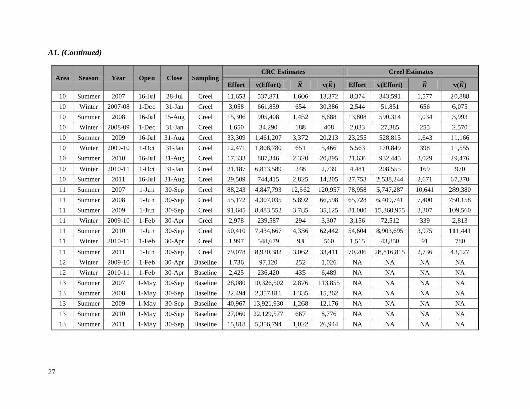
A1. CRC-based and creel-based estimates of effort (angler trips) total Chinook harvest ( )

by fishery .......................................................................................................................................... 25

A2. CRC Species Composition: Area 10 Winter Discrepancies .................................................... 28

A3. Evaluation product method assumptions ................................................................................... 31

A4. CRC-based and creel-based estimates of total Chinook encounters by fishery estimated

using a bias-corrected M2 approach ........................................................................................... 35

A5. Sampling data required for M1 and M2 estimates of Chinook encounters for fisheries

sampled using Baseline Sampling. ............................................................................................... 37

A6. Chinook encounters and mortality by size and mark-status for fisheries sampled using

Baseline Sampling. ......................................................................................................................... 37

iv

LIST OF TABLES

Table 1. Summary of Chinook MSFs in Puget Sound in which PSSU had conducted

Baseline Sampling. .....................................................................................................4

Table 2. CRC-based Chinook harvest estimates, VTR encounters by size and mark-

status, estimated CV of total encounters estimates and recommended

methodology for estimation of total Chinook encounters. ........................................18

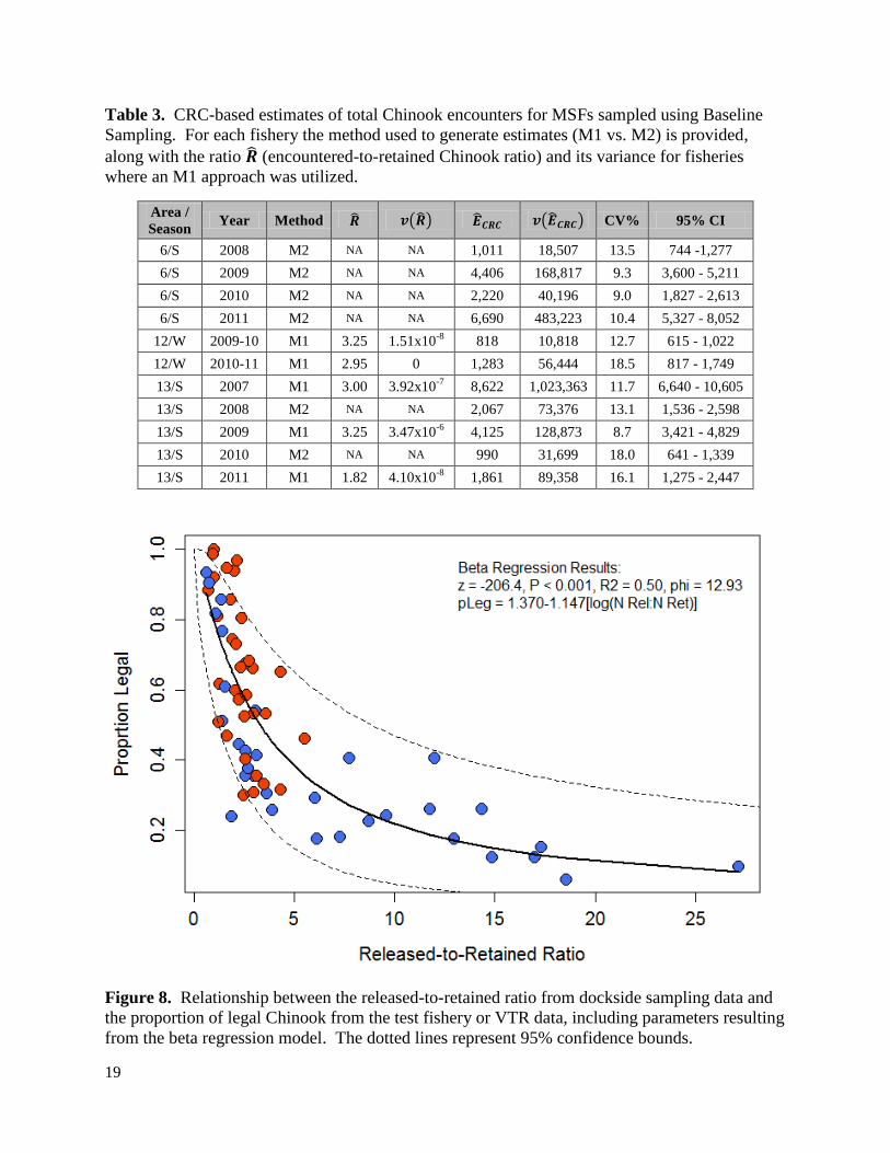
Table 3. CRC-based estimates of total Chinook encounters for fisheries sampled using

Baseline Sampling. For each fishery the method used to generate estimates (M1

vs. M2) is provided, along with the ratio (encountered-to-retained Chinook

ratio) and its variance for fisheries where an M1 approach was utilized..................19

Table 4. Size and mark-status proportions used to apportion CRC-based estimates of

total Chinook encounters into size and mark-status groups. Data source denotes

whether the proportions were derived from VTR data or by the product method

using dockside sampling data (DS)...........................................................................20

Table A2.1 Summary of creel-based and CRC-based total Chinook harvest estimates during

Area 10 winter MSFs that occurred in October and November. CRC-based

estimates were estimated in two ways: (1) using species compositions from the

Puget Sound Sampling Program (2) replacing October and November species

compositions with those reported in CRCs. ..............................................................28

v

LIST OF FIGURES

Figure 1. Map of Western Washington, showing the Marine Catch Areas of Puget

Sound (Areas 5 through 13) and the Washington Coast (Areas 1 through 4). ........3

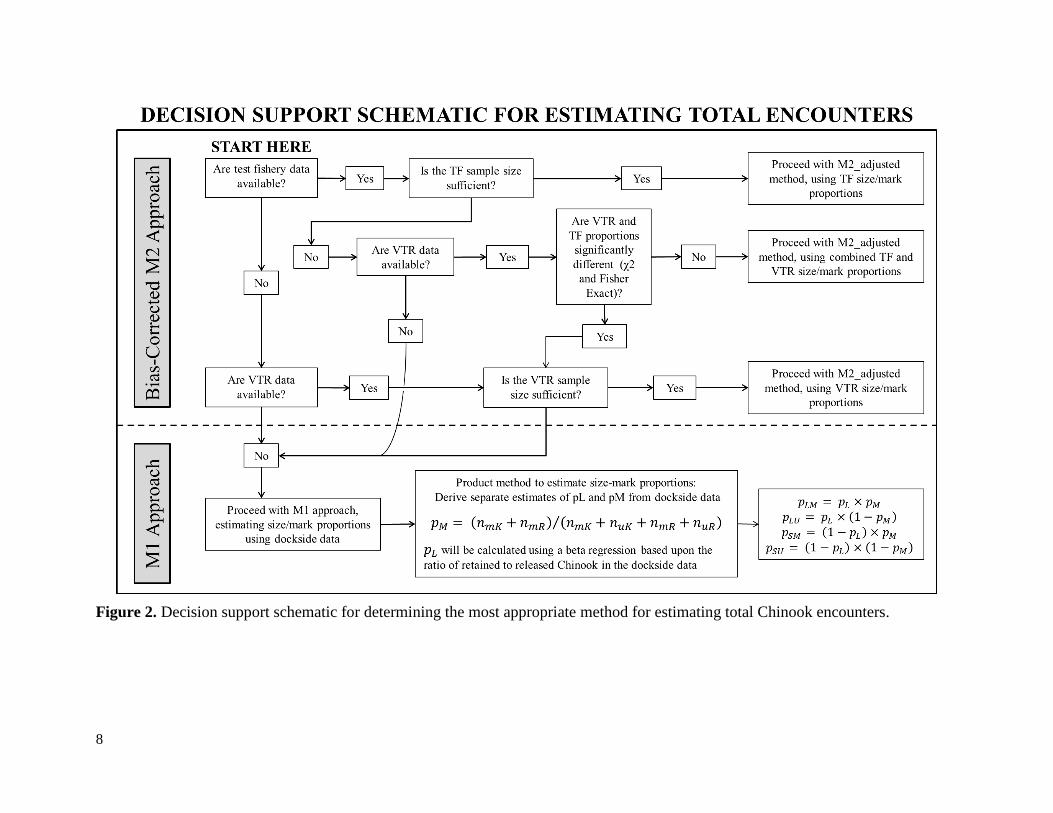
Figure 2. Decision support schematic for determining the most appropriate method for

estimating total Chinook encounters. .......................................................................8

Figure 3. Boxplots depicting the ratio of estimated CRC harvest to creel harvest for

each fishery by marine area. Black bars denote the median while the upper

and lower bounds of the boxes represent the first and third quartiles.

Whiskers represent the minimum and maximum values within 1.5 IQR

(interquartile range) of the box bounds and outliers are any points beyond the

whiskers. The horizontal dotted line represents a 1-to-1 relationship between

the two estimates. ...................................................................................................13

Figure 4. Comparison of CRC versus creel Chinook harvest estimates (# of fish) for all

Puget Sound Chinook MSFs that were comprehensively monitored between

2003 and 2011. The dotted line is the line of unity where both harvest

estimates are equal; the solid red line is the regression described by the

equation in the upper left corner. CRC areas are indicated by numbers in

circles. ....................................................................................................................14

Figure 5. Boxplots depicting the ratio of CRC-based to creel-based M2 estimates of

total Chinook encounters for each fishery by marine catch area. Black bars

denote the median while the upper and lower bounds of the boxes represent

the first and third quartiles. Whiskers represent the minimum and maximum

values within 1.5 IQR (interquartile range) of the box bounds and outliers are

any points beyond the whiskers. The horizontal dotted line represents a 1-to-1

relationship between the two estimates..................................................................15

Figure 6. Comparison of CRC-based versus creel-based M2 estimates of total Chinook

encounters for all Puget Sound Chinook MSFs that were comprehensively

monitored between 2003 and 2011. The dotted line is the line of unity where

both estimates are equal; the solid red line is the regression described by the


circles. ....................................................................................................................16

Figure 7. Comparison of CRC-M1 versus creel-M2 total Chinook encounters estimates

for all Puget Sound Chinook MSFs that were comprehensively monitored

between 2003 and 2011. The dotted line is the line of unity where both

estimates are equal; the solid red line is the regression described by the


circles. ....................................................................................................................17

Figure 8. Plot of the relationship between the released-to-retained ratio from dockside

sampling data and the proportion of legal Chinook from the test fishery or

VTR data, including parameters resulting from the beta regression model in

addition to 95% confidence bounds. ......................................................................19

vi

Figure A2.1 Boxplots depicting the ratio of CRC harvest to creel harvest for each fishery

by marine catch area, before species composition adjustments in Area 10.

Black bars denote the median while the upper and lower bounds of the boxes

represent the first and third quartiles. Whiskers represent the minimum and

maximum values within 1.5 IQR (interquartile range) of the box bounds and

outliers are any points beyond the whiskers. The horizontal dotted line

represents a 1-to-1 relationship between the two estimates. ..................................29

Figure A2.2 Boxplots depicting the ratio of CRC Chinook harvest to creel Chinook harvest

by month in Area 10 MSFs before species composition updates. Black bars






Figure A2.3 Boxplots depicting the ratio of CRC Chinook harvest to creel Chinook harvest

by month in Area 10 MSFs after species composition updates. Black bars






Figure A2.4 Boxplots depicting the ratio of CRC harvest to creel harvest for each fishery

by marine catch area, after species composition adjustments in Area 10.

Black bars denote the median while the upper and lower bounds of the boxes

represent the first and third quartiles. Whiskers represent the minimum and

maximum values within 1.5 IQR (interquartile range) of the box bounds and

outliers are any points beyond the whiskers. The horizontal dotted line

represents a 1-to-1 relationship between the two estimates. ..................................30

Figure A3.1 Assessment of accuracy of mark rates estimated from dockside data relative to

values derived from on-the-water sampling (test fishery and VTR; assumed to

be correct). Regression-based comparisons for pooled (A) and season-specific

(B) mark rate estimates, relative to hypothesized equality (i.e., the diagonal

reference line). (C) Mark rate difference (creel minus on-the-water estimate)

as a function of on-the-water mark rate. (D) Mean absolute difference of creel

and on-the-water mark rate estimates. In A-C, red denotes summer whereas

blue denotes winter and numbers correspond to catch record card reporting

areas. Regression lines and confidence intervals (95%) are displayed where

significant (P < 0.05) relationships were detected. ............................................... 32

Figure A3.2 Evaluation of assumption of similar for legal and sublegal fish (A),

similar for marked and unmarked fish (B), and comparison of

calculated via the product method and computed based on actual observations.

In all figures, red denotes summer whereas blue denotes winter, the diagonal

line is the reference for hypothesized equality, and regression lines and 95%

confidence intervals are displayed where significant (P < 0.05) relationships

were detected. ....................................................................................................... 34

1

INTRODUCTION

Background and Fishery Context

Based on agreements between the State of Washington and the Northwest Treaty Tribes, the

Washington Department of Fish and Wildlife (WDFW) has been conducting pilot1 recreational

mark-selective Chinook fisheries (MSFs) in the marine catch areas of Puget Sound since 2003.

The goal of these fisheries is to allow increased angler opportunities on hatchery-raised, marked

(adipose fin-clipped) salmon while limiting impacts on unmarked (adipose fin intact; typically

wild origin) stocks of conservation concern, particularly ESA-listed Puget Sound Chinook.

Given that anglers will encounter and then release unmarked Chinook during MSFs, execution of

proper sampling and monitoring strategies is critical in order to assess catch rates and estimate

impacts on wild stocks.

WDFW implemented the first recreational Chinook MSFs in the marine waters of Washington

State in Areas 5 and 6 (Strait of Juan de Fuca) during summer 2003. In subsequent years,

WDFW has implemented additional pilot-level MSFs in other Puget Sound marine catch areas

(Areas 7 through 13; Figure 1) during both the summer and winter seasons (see Appendix A in

WDFW 2012 for a list of areas and seasons). For example, the first winter MSFs were

established in Areas 8-1 and 8-2 from October 2005 through April 2006 and have continued each

winter season since. Additionally, beginning in 2007, summer MSFs were established in Areas

9, 10, 11 and 13 and winter MSFs began in Areas 7, 9 and 10. During the winter of 2010

(February through April), Chinook MSFs occurred for the first time in Areas 11 and 12 and have

continued each year thereafter. Similarly, beginning in the summer of 2012, a Chinook MSF

was established in Area 12 (South of Ayock Point), from July 1 through October 15. This steady

introduction of new fisheries has resulted in an increase in angler participation in MSFs from an

estimated 24,593 angler trips during the 2003-04 fishing season to more than 150,000 angler

trips during the 2012-13 fishing season.

Sampling and Monitoring Program

Given the pilot nature of the Chinook MSFs in Puget Sound, WDFW’s Puget Sound Sampling

Unit (PSSU) has been tasked with implementing a comprehensive monitoring program to collect

the data needed to evaluate the impacts of MSFs on unmarked salmon. To monitor each fishery,

PSSU implements one of the four following sampling designs: i) Full Murthy Estimate Design,

ii) Reduced Murthy Estimate Design, iii) Aerial-Access Design or iv) Baseline Sampling Design.

The design selected depends on area and season considerations, the magnitude of the fishery and

State-Tribal agreements made prior to the start of the fishing season. For a complete description

of the methods associated with these sampling designs, see WDFW’s “Methods Report:

Monitoring Mark-Selective Recreational Chinook Fisheries in the Marine Catch Areas of Puget

Sound (Areas 5 through 13),” available at http://www.wdfw.wa.gov/publications/01357/.

1 As stated in state-tribal agreement documents (e.g., WDFW and NWIFC 2009): “The purpose of the ‘pilot’ fishery is to collect

information necessary to enable evaluation and planning of potential future mark-selective fisheries. The ‘pilot’ fishery provides

a basis for determining if the data needed to estimate critical parameters can be collected and if the sample sizes needed to

produce these estimates with agreed levels of precision can be realistically obtained.”

http://www.wdfw.wa.gov/publications/01357/

2

Three of the above-mentioned designs (all except Baseline Sampling) are characterized as

comprehensive, “intensive” monitoring programs, consisting of all or a subset of the following

components:

1. Intensive dockside creel sampling to provide in-season estimates of effort (number of

anglers and boats) and retained and released Chinook (including number of marked and

unmarked);

2. Effort surveys (aerial or on-the-water surveys) to provide information on the proportion

of effort originating from sampled sites;

3. Test fishing and/or an expanded Voluntary Trip Report (VTR) program to provide

information on the size/mark-status composition of the population of fish being

encountered.

PSSU has tailored each of the comprehensive monitoring programs to reliably estimate the

following critical parameters needed for evaluating mark-selective fisheries: i) the mark rate of

the targeted Chinook population, ii) the total number of Chinook salmon harvested (by size

[legal or sublegal] and mark-status [marked or unmarked] group), iii) the total number of

Chinook salmon released (by size and mark-status group), iv) the coded-wire tag- (CWT) and

sometimes DNA-based stock composition of marked and unmarked Chinook mortalities, and v)

the total mortality of marked and unmarked double index tag (DIT) CWT stocks. In addition,

PSSU has acquired and analyzed relevant data characterizing other aspects of the pilot MSFs,

including descriptors of fishing effort, fishing success (catch [landed Chinook] per unit effort),

recreational fishing methods, the length and age composition of encountered Chinook, and the

overall intensity of our sampling efforts. As such, the data collected through these

comprehensive monitoring programs allow biologists to produce weekly in-season estimates and

timely finalized post-season estimates of effort, catch, total encounters and fishery impacts.

The fourth sampling design, Baseline Sampling, is a scaled-back monitoring program that is

currently implemented in lower-magnitude MSFs (and year-round in non-selective sport

fisheries) throughout Puget Sound.

Table 1 presents a summary of the MSFs, by area and season in which PSSU has conducted

Baseline Sampling. Samplers collect data on salmon catch (retained and released) and angler

effort via dockside angler interviews and obtain on-water encounter rate data through distributing

and collecting voluntary trip reports (VTR) from private anglers. In contrast to the three

comprehensive monitoring programs mentioned above, the data collected through Baseline

Sampling does not allow for in-season or immediate post-season estimates of angler effort,

landed catch, total encounters, or fishery impacts. While the Catch Record Card (CRC)2 system

provides post-season estimates (approximately one year after the fishery) of angler effort and

landed Chinook harvest in these MSFs, to date there has not been a method developed for

estimating total encounters and release mortalities of unmarked Chinook in these fisheries.

Affected fisheries include MSFs in Areas 6, 12 and 13 during the summer and Area 12 during

the winter (Table 1).

2 See Conrad and Alexandersdottir (1993) for an overview of the CRC system.

3

Figure 1. Map of Western Washington, showing the Marine Catch Areas of Puget Sound (Areas

5 through 13) and the Washington Coast (Areas 1 through 4).

Columbia River

4

Table 1. Summary of Chinook MSFs in Puget Sound in which PSSU had conducted Baseline

Sampling.

Catch Area Season Year Dates Sampling Design

6 Summer

2008 Jul 1 – Aug 9

Baseline

sampling, VTRs,

CRC estimates

2009 Jul 1 – Aug 6

2010 Jul 1 – Aug 15

2011 Jul 1 – Aug 15

2012 Jul 1 – Aug 15

2013 Jul 1 – Aug 15

12 (S of

Ayock Pt) Summer

2012 Jul 1 – Oct 15

2013 Jul 1 – Oct 15

12 Winter

2009-10 Feb 1 – Apr 30

2010-11 Feb 1 – Apr 30

2011-12 Feb 1 – Apr 30

2012-13 Oct 16 – Dec 31

& Feb 1 – Apr 30

13 Summer

2007 May 1 – Sep 30

2008 May 1 – Sep 30

2009 May 1 – Sep 30

2010 May 1 – Sep 30

2011 May 1 – Sep 30

2012 May 1 – Sep 30

2013 May 1 – Sep 30

‘CRC for Encounters’ Workgroup

To address the need for an agreed-to encounters estimation methodology for the Baseline-

sampled MSFs (Table 1), the NWIFC and WDFW created a joint work group to develop a

method for estimating total Chinook encounters and release mortalities in these MSFs. Periodic

meetings of this ‘CRC for Encounters’ technical workgroup started in May 2011 and concluded

in September 2013, when the new encounters estimation method was finalized. The primary

goal and objectives of the workgroup were as follows:

Goal: Estimate total Chinook encounters and mortalities for Puget Sound MSFs that rely

on the CRC system for harvest estimates and are sampled on a Baseline level only.

Objectives: Identify the most accurate (least biased, most precise) method for estimating

encounters from CRC estimates. Apply this method to produce estimates of total

Chinook encounters (ultimately mortalities) by size/mark-status group (legal-marked,

legal-unmarked, sublegal-marked, sublegal-unmarked) when the only data available for a

given Chinook MSF are: i) CRC estimates of total landed catch, ii) Baseline interview

5

data on retained and released salmon encounters and iii) (if available) on-the-water logs

of salmon encounters supplied by anglers.

The workgroup’s approach was informed by existing data and estimation approaches,

specifically Conrad and McHugh’s (2008) agreed-to method for estimating total Chinook

encounters by size and mark-status for intensively-monitored Chinook MSFs in Puget Sound.

Conrad and McHugh describe two methods for estimating total Chinook encounters:

Method 1 (M1) estimates of total Chinook encounters are obtained by summing estimates

of catch, based on sampled landings, and releases, based on values reported by anglers

during interviews, generated from the creel survey design.

Method 2 (M2) estimates of total Chinook encounters are obtained by dividing an

estimate of total legal-marked (LM) Chinook harvest by the proportion of LM Chinook

present in the targeted population, derived from test fishing or VTR data. This approach

attempts to eliminate bias arising from recall error in angler-reported releases.

While both the M1 and M2 approaches are designed to estimate the same parameter, Conrad and

McHugh (2008) ultimately recommend the M2 approach, with a bias correction that accounts for

intentional and unintentional releases of LM Chinook.

Both methods require an estimate of total Chinook harvest, which cannot be produced using data

collected through Baseline Sampling. Fishery-total estimates of catch and effort are eventually

available (approximately one year after the close of the fishery) through WDFW’s CRC system.

The estimation framework developed in this report allows for the generation of M1 and M2

estimates of total Chinook encounters using CRC estimates of Chinook harvest as the primary

building block. Before proceeding, however, it was necessary to evaluate the accuracy of the

CRC-based harvest estimates.

Report Intent

The intention of this report is to document the methods, results, conclusions and

recommendations resulting from the CRC for Encounters workgroup’s efforts to identify a

suitable method for estimating the total number of Chinook salmon encountered by size/mark-

status category in a given MSF where the less intensive Baseline Sampling design is

implemented and CRC estimates of landed catch are produced. The Methods section provides an

overview of the encounters from CRC estimation scheme including: i) Description of available

data, ii) Validation of catch record card Chinook harvest estimates, iii) Decision support tool for

data analysis and iv) Estimators for total encounters, including associated assumptions. The

Results section includes: i) Outcome of the validation of catch record card Chinook harvest

estimates, ii) Validation of proposed encounters estimators and iii) Estimates resulting from

application of the new method to Baseline-sampled MSFs in Areas 6, 12 and 13. Finally, the

Discussion section provides further explanation and context for the observed results, discussion

of the assumptions, cautions and caveats that accompany using the new method, as well as

recommendations of the CRC for Encounters workgroup as the method is applied moving

forward.

6

METHODS

Description of Available Data

Conrad and McHugh (2008) provided two methods for estimating total encounters in Puget

Sound Chinook MSFs. The first method, M1, requires estimates of retained and released

Chinook generated from the creel survey design which includes dockside sampling and angler

interview data. A critical assumption of this method is that anglers accurately recall and report

all Chinook that were encountered and released. The second method, M2, requires an estimate

of LM (legal-sized and marked) Chinook harvest and an independent estimate of the proportion

of LM fish in the population being targeted, derived from test fishing or VTR data. This method

assumes that all LM Chinook that are encountered by anglers are retained. After a rigorous bias

analysis, Conrad and McHugh (2008) recommended the M2 approach over the M1 approach and

suggested a bias-correction factor of 0.13 to account for the intentional and unintentional release

of LM Chinook.

Test fishing or VTR data (given a sufficient sample size, discussed below) are required in order

to proceed with an M2 approach. These data sets provide counts of Chinook encountered by size

and mark-status group. All fish that are brought to the boat are designated into one of four

groups: legal-marked (LM), legal-unmarked (LU), sublegal-marked (SM), and sublegal-

unmarked (SU). These counts are used to estimate the proportion of fish in the population being

targeted that is both legal and marked. Currently, test fishing is conducted only in the Areas 9

and 10 (summer and winter) and Area 7 (winter) Chinook MSFs, all of which are sampled using

one of the comprehensive monitoring programs. VTRs are distributed and collected by dockside

samplers during all Puget Sound MSFs, however, angler participation varies significantly by

area. In order to proceed with an M2 approach, these data need to meet minimum sample size

requirements (see below).

Dockside sampling and angler interview data are an essential element in estimating total

Chinook encounters, particularly if small test fishery or VTR sample sizes require an M1

approach. At designated sites on sample days, samplers attempt to intercept all anglers returning

from a given fishery, recording the size and mark-status of their catch and the angler-reported

number of Chinook released by mark-status (marked, unmarked, unknown). As there is

generally a small proportion of Chinook harvest that is sublegal and/or unmarked, information on

the size and mark-status composition of sampled catch can be used to estimate the LM Chinook

harvest based on total Chinook harvest estimates provided by CRCs.

For fisheries monitored using Baseline Sampling, fishery-total Chinook harvest estimates are a

critical data component required to estimate total Chinook encounters. As discussed above,

these are available through the WDFW CRC system, which can provide fishery-specific

estimates of total Chinook harvest, with associated variance. These estimates are a building

block in the estimation of total Chinook encounters, regardless of whether an M1- or M2-based

approach is utilized.

7

Validation of Catch Record Card Chinook Harvest Estimates

Upon purchasing a state fishing license, anglers are provided with a Catch Record Card that they

are required to complete and return at the end of the fishing year. For every salmon harvested,

the angler provides the catch area, date, species and mark-status. This information is compiled

by WDFW and used to produce estimates of total salmon harvest by catch area and statistical

week or month. To adjust for non-response bias, correction factors of 1.00 and 0.68 are applied

to estimates in Marine Area 5 and Marine Areas 6-13, respectively, as described in Conrad and

Alexandersdottir (1993). Effort (in angler trips) is estimated by dividing CRC-based salmon

harvest estimates by the catch-per-unit-effort (CPUE) from dockside sampling data for the

area/time period of interest. Total salmon harvest can then be apportioned into species-specific

harvest estimates using species composition proportions from dockside sampling observations.

These species compositions are used instead of those reported on CRCs under the assumption

that they provide a more accurate representation due to more accurate species identification by

trained samplers than by the general fishing public. For full details on the estimation of salmon

harvest using CRCs see Conrad and Alexandersdottir (1993).

As more than 20 years have passed since the non-response bias correction factors were produced,

it was necessary to evaluate recent CRC estimates to ensure that they continue to produce valid,

statistically accurate harvest estimates. To accomplish this evaluation, in an approach similar to

that of Conrad and Alexandersdottir (1993), we compared the bias-corrected CRC-based

estimates of Chinook harvest to independently derived Chinook harvest estimates from intensive

creel surveys for all Puget Sound MSFs that have been comprehensively monitored. In these

comparisons it was assumed that the estimates provided by the creel surveys were unbiased.

Since the start and end dates of each MSF did not always coincide with time strata in the

standard CRC reporting process, separate estimates of Chinook harvest were produced that

match the specific dates of each Puget Sound MSF, beginning with the summer 2003 season

through the summer 2011 season (the most recent CRC estimates that are available). These

estimates were then paired with complementary creel survey estimates. Our full analysis of

these comparisons is presented in the Results section and in Appendix A1.

Methods Determination Scheme

We propose the following decision support schematic as a guide in determining the most

appropriate method for estimating total Chinook encounters in MSFs (Figure 2). For all

fisheries, it is assumed that a CRC-based estimate of Chinook harvest is available. The

availability of other data will vary by fishery, which will ultimately determine the method used

to estimate total Chinook encounters.

Given past work, the preferred methodology is the M2-based approach, using test fishing data to

estimate the proportion of LM fish (pLM) in the target population. Test fishing data are believed

to be of higher quality than VTR data, as they are collected by trained samplers. When these

data are available, it is important to ensure that sample sizes are sufficient to meet precision

requirements. As a guideline, we recommend a coefficient of variation threshold of 20% around

M2 total encounters estimates. If test fishing sample sizes are insufficient, they can be combined

with VTR data if χ2 tests indicate that the proportions of the two data sets are not significantly

different. In situations where the CV is greater than 20% an M1 approach should be employed.

8

Figure 2. Decision support schematic for determining the most appropriate method for estimating total Chinook encounters.

9

If test fishing data do not exist for a given fishery, which is the case for past fisheries and has

necessitated the development of the CRC for Encounters framework, or if sample sizes are too

small and cannot be combined with VTR data, the next best option is to use a bias-corrected M2

approach and estimate pLM using only VTR data. Again, it is essential to evaluate sample sizes

to ensure the precision around total encounters estimates will be acceptable (target CV = 20%).

Finally, if test fishing or VTR data are not available in sufficient sample sizes, an analog to the

M1 approach is recommended. In this case the relationship between the number of Chinook

encountered and retained in dockside sampling and angler interview data is used to estimate total

encounters. Since test fishing or VTR data are unavailable, estimates of the size/mark-status

composition will need to be derived using an alternate data source. The methods developed to

provide alternate estimates of size/mark-status composition are described below.

Encounters Estimators

M2 Estimator:

Given a sufficient sample size of test fishery or VTR (or a combination) data, the proportion of

fish that belongs to each size/mark-status group can be estimated by applying the same methods

used for intensive creel studies as outlined in the WDFW Methods Report (WDFW 2012).

The M2 approach requires an estimate of LM Chinook harvest, which can be derived by

apportioning the CRC-based estimate of total Chinook harvest into size and mark-status groups

using proportions ( ) from the dockside sampled catch as follows:

(1) ( )⁄

(2) ( ) [ ( )] ( )⁄

where X=legal (L) or sublegal (S), Y=marked (M) or unmarked (U), and subscript K indicates

kept. and are season total dockside counts of landed fish and the subset of fish in a

given size/mark-status group.

Estimates of harvest by size/mark-status and associated variances are calculated as:

(3)

(4) ( ) ( )

( ) ( ) ( )

where is the CRC-based estimate of total Chinook harvest.

With an estimate of legal-marked Chinook harvest, the bias-corrected M2 estimate of total

Chinook encounters and its variance is calculated as:

(5) [ ( )]⁄

(6) ( ) ( ) ( ( )

( )

( )

( )

)

10

where is the proportion of LM fish in the target population and is the bias correction

factor to account for encountered LM Chinook that are released (estimated at 0.13 by Conrad and

McHugh 2008) which is treated as a known constant with no variance.

Finally, total estimated Chinook encounters can be apportioned into the four size/mark-status

groups and associated mortalities can be calculated as described in the WDFW Methods Report

(WDFW 2012).

M1 Estimator:

If the available data do not permit an M2 approach, we can estimate total Chinook encounters

using an M1 approach. First we calculate the number of retained (kept) and released Chinook in

the dockside sampling and angler interview data. The number of retained Chinook is calculated

as:

(7)

where is the number of marked Chinook retained, is the number of unmarked Chinook

retained, and the DS subscript indicates that the sample data are from dockside sampling.

The dockside interview data includes a field for released salmon of unknown species, which

needs to be incorporated into estimates of released Chinook. To do this we estimate the

proportion of all released salmon of known species that are Chinook and its variance and

apportion the number of released unidentified salmon accordingly.

(8) ( ) ( )⁄

(9) ( ) ( ( )) ( )⁄

where , and are the number of Chinook reported released that were of marked,

unmarked and unknown mark-status, and is the number of other salmon (positively

identified species other than Chinook) reported released.

With an estimate of , we estimate the number of released Chinook and its variance as:

(10) ( ) ( )

(11) ( ) ( )

where is the number of unknown (species) salmon released.

To estimate total Chinook encounters, we first calculate the ratio ( ) of encountered Chinook to

retained Chinook in the dockside sampling and interview data and its variance:

(12) ⁄

(13) ( ) ( ( ) ⁄ )

where is the estimated number of encounters in the dockside data ( ) during the

given fishery. Since is a count with no associated variance, ( ) ( ).

11

The ratio, , is then applied to the CRC-based estimate of harvested Chinook to provide an M1

estimate of total Chinook encounters:

(14)

with estimated variance:

(15) ( ) ( ) ( ) ( ) ( )

To apportion the estimate of total Chinook encounters into size/mark-status groups, estimates of

the proportion of each group present in the target population are needed. Given that an M1

approach is being used, this information is not available through test fishery or VTR data and

must be derived using an alternate data source. To determine the proportion of each group, we

recommend a product method, where the mark-rate ( ) and legal proportion ( ) are estimated

independently and combined to provide an estimate of the proportion for each group as follows:

(16)

(17) ( ) (18) ( )

(19) ( ) ( )

where the variance for each estimated proportion is equivalent to:

(20) ( ) ( )

( ) ( ) ( )

The proportion of encounters that are marked ( ) can be estimated using the dockside sampling

and angler interview data. First, released Chinook of unknown mark-status, as well as

unidentified salmon releases, are apportioned into the and categories based on known

species and mark-status composition reported to have been released. The proportion of

encounters that are marked is then calculated by:

(21) ( ) ( )⁄

where and include the apportioned Chinook of unknown mark-status and unidentified

salmon that were reported released. The variance of is computed as:

(22) ( ) ( ( )) ( )⁄

where n is the total number of Chinook encounters from the dockside sampling and angler

interview data.

The proportion of encounters that are legal-sized ( ) will be estimated based on the relationship

between test fishery and/or VTR estimates of this parameter and dockside interview-based

estimates of released-to-retained Chinook fitted to data from past MSFs that were intensively

monitored. In this situation linear regression is unsuitable given the existence of observations

near the bounds of 0 and 1 and high variability in dockside interview data, as it would yield

predictions outside the range of possibilities. Thus, we used a beta regression, which is

commonly used to model variables that assume values in the standard unit interval (Cribari-Neto

and Zeileis 2010). The predictor variable is the ratio of released to retained Chinook (loge-

transformed), computed from dockside creel data, and the response is the fraction of total test

fishery or VTR encounters that are legal in size for each Puget Sound Chinook MSF (through the

12

summer of 2012). Within the beta regression model we used a logit link function and weighted

the data by the total number of test fishery or VTR encounters.

This model yields estimates of intercept ( ), slope ( ) and precision ( ) parameters of the

relationship between and ( ⁄ ), which can be used to generate predictions for

new fisheries as follows:

(23) ( ) ( ( ))⁄

where ( ) is a linear function of the form:

(24) ( ) [ ( ⁄ )]

The variance of predictions will be estimated as:

(25) ( ) ( ( )) ( )⁄

In order for the product method to provide reliable estimates of the size/mark-status proportions

in a fishery, two key assumptions need to be met: (1) dockside interview-based estimates of the

proportion of encounters that are marked and model-predicted estimates of the proportion of

encounters that are legal need to be accurate, and (2) mark rates need to be similar for legal and

sublegal size classes and the size composition needs to be similar for marked and unmarked fish,

(i.e., statistical independence of and ). Although these assumptions will likely be violated

in some years/fisheries, an analysis of available data suggests that they are well met on average

(Appendix A3).

Estimates of Chinook retention by size and mark-status can be derived using the same methods

from the M2 estimator (Equations 1-4). Lastly, estimates of Chinook releases and associated

mortalities can be calculated as described in the WDFW Methods Report (WDFW 2012).

13

RESULTS

Validation of Catch Record Card Chinook Harvest Estimates

Upon initial inspection, an anomalously large discrepancy was observed between CRC and creel

harvest estimates during some winter MSFs in Area 10. We hypothesized that this discrepancy

may be caused by an extensive shore-based angling effort targeting chum during October and

November in Area 10. While captured in the CRC data, this chum harvest may not be accurately

accounted for in the sampling data, resulting in an inflated Chinook harvest estimate when CRC-

based total salmon harvest estimates are apportioned using PSSU species composition. To solve

this problem, we replaced the PSSU species compositions with those from the CRCs during the

months of October and November in Area 10 (see Appendix A2 for full discussion on this topic).

As an initial comparison, we calculated the ratio of CRC to creel Chinook harvest for each

fishery. For all 55 MSFs where both CRC and creel harvest estimates existed, the mean ratio

was 1.10 (SD = 0.287). Boxplots of the ratio for each fishery show a relative consistency across

areas, ranging mostly between 0.8 and 1.5 (Figure 3). We also plotted CRC harvest estimates

against creel harvest estimates (Figure 4). This view of the data clearly illustrates that the

magnitude of harvest in summer fisheries is typically much higher than that of winter fisheries.

While they generally match well with the creel estimates, there appears to be a slight positive

bias in the CRC harvest estimates, which becomes more prominent with increasing harvest.

Figure 3. Boxplots depicting the ratio of estimated CRC harvest to creel harvest for each fishery

by marine area. Black bars denote the median while the upper and lower bounds of the boxes

represent the first and third quartiles. Whiskers represent the minimum and maximum values

within 1.5 IQR (interquartile range) of the box bounds and outliers are any points beyond the

whiskers. The horizontal dotted line represents a 1-to-1 relationship between the two estimates.

14

Figure 4. Comparison of CRC versus creel Chinook harvest estimates (# of fish) for all Puget Sound Chinook MSFs that were

comprehensively monitored between 2003 and 2011. The dotted line is the line of unity where both harvest estimates are equal; the

solid red line is the regression described by the equation in the upper left corner. CRC areas are indicated by numbers in circles.

15

Validation of Encounters Estimators: Comparison with Existing Creel Estimates

For areas that were comprehensively monitored and creel-based total encounters estimates have

been provided, we estimated CRC-based total encounters using both the M2 and M1 estimators

(Appendix A4). We calculated the ratio of CRC-based M2 total encounters to creel-based total

encounters for each fishery. For all 55 MSFs where both CRC and creel estimates of total

Chinook encounters existed, the mean ratio was 1.09 (SD = 0.301). Boxplots of the ratio for

each fishery show a relative consistency across areas, ranging mostly between 0.8 and 1.4

(Figure 5). CRC-based total encounters estimates derived from both the M2 (Figure 6) and M1

(Figure 7) estimators were also plotted against and compared with creel-based total encounters

estimates.

Figure 5. Boxplots depicting the ratio of CRC-based to creel-based M2 estimates of total

Chinook encounters for each MSF by marine catch area in Puget Sound. Black bars denote the

median while the upper and lower bounds of the boxes represent the first and third quartiles.

Whiskers represent the minimum and maximum values within 1.5 IQR (interquartile range) of

the box bounds and outliers are any points beyond the whiskers. The horizontal dotted line

represents a 1-to-1 relationship between the two estimates.

16

Figure 6. Comparison of CRC-based versus creel-based M2 estimates of total Chinook encounters for all Puget Sound Chinook MSFs

that were comprehensively monitored between 2003 and 2011. The dotted line is the line of unity where both estimates are equal; the

solid red line is the regression described by the equation in the upper left corner. CRC areas are indicated by numbers in circles.

17

Figure 7. Comparison of CRC-M1 versus creel-M2 total Chinook encounters estimates for all Puget Sound Chinook MSFs that were

comprehensively monitored between 2003 and 2011. The dotted line is the line of unity where both estimates are equal; the solid red

line is the regression described by the equation in the upper left corner. CRC areas are indicated by numbers in circles.

18

Application of Methods: Total Encounters Estimates in Areas without Creel Estimates

For the Areas 6, 12 and 13 MSFs that have been monitored using Baseline Sampling and have no

existing estimates of total encounters, we used CRC harvest estimates and VTR encounters to

estimate the CV of bias-corrected M2 total encounters estimates using equations provided in the

WDFW Methods Report (WDFW 2012). Considering these CV estimates and based on a

threshold of 20%, the most appropriate methodology for generating total Chinook encounters

estimates based on the available data is recommended in Table 2. CRC-based estimates of total

Chinook encounters are provided in Table 3 along with the method used to generate them.

In order to estimate size/mark-status proportions for a given fishery using the product method,

we used equations 21-25 to predict both and . A graphical representation of the beta

regression analysis is provided in Figure 8, which yielded intercept, slope and precision

parameters of =1.370, =1.147 and =12.93. The proportions used to allocate total

encounters estimates into the four size/mark-status groups, and the data source that they were

derived from, are provided in Table 4.

A summary of the sampling data available for the CRC-M1 and CRC-M2 estimates of total

Chinook encounters for MSFs in Areas 6, 12 and 13 is presented in Appendix Table A5.

Appendix Table A6 reports estimates of total Chinook retained and released by size and mark-

status categories using the recommended estimation method for these fisheries.

Table 2. CRC-based Chinook harvest estimates, VTR encounters by size and mark-status,

estimated CV of total encounters estimates and recommended methodology for estimation of

total Chinook encounters.

Area /

Season Year ( ) LM LU SM SU

Est.

CV% Method

6/S 2008 537 3,840 81 50 0 2 13.5 M2

6/S 2009 2,372 29,988 117 53 10 12 9.3 M2

6/S 2010 1,400 12,932 179 61 5 3 9.0 M2

6/S 2011 3,320 79,356 126 60 25 18 10.4 M2

12/W 2009-10 252 1,026 2 6 8 4 69.4 M1

12/W 2010-11 435 6,489 6 2 9 6 39.8 M1

13/S 2007 2,876 113,855 12 11 28 4 28.1 M1

13/S 2008 1,335 15,262 31 4 5 2 13.1 M2

13/S 2009 1,268 12,176 13 9 12 2 24.0 M1

13/S 2010 667 8,776 21 3 3 1 17.8 M2

13/S 2011 1,022 26,944 12 8 0 1 25.0 M1

19

Table 3. CRC-based estimates of total Chinook encounters for MSFs sampled using Baseline

Sampling. For each fishery the method used to generate estimates (M1 vs. M2) is provided,

along with the ratio (encountered-to-retained Chinook ratio) and its variance for fisheries

where an M1 approach was utilized.

Area /

Season Year Method ( ) ( ) CV% 95% CI

6/S 2008 M2 NA NA 1,011 18,507 13.5 744 -1,277

6/S 2009 M2 NA NA 4,406 168,817 9.3 3,600 - 5,211

6/S 2010 M2 NA NA 2,220 40,196 9.0 1,827 - 2,613

6/S 2011 M2 NA NA 6,690 483,223 10.4 5,327 - 8,052

12/W 2009-10 M1 3.25 1.51x10-8

818 10,818 12.7 615 - 1,022

12/W 2010-11 M1 2.95 0 1,283 56,444 18.5 817 - 1,749

13/S 2007 M1 3.00 3.92x10-7

8,622 1,023,363 11.7 6,640 - 10,605

13/S 2008 M2 NA NA 2,067 73,376 13.1 1,536 - 2,598

13/S 2009 M1 3.25 3.47x10-6

4,125 128,873 8.7 3,421 - 4,829

13/S 2010 M2 NA NA 990 31,699 18.0 641 - 1,339

13/S 2011 M1 1.82 4.10x10-8

1,861 89,358 16.1 1,275 - 2,447

Figure 8. Relationship between the released-to-retained ratio from dockside sampling data and

the proportion of legal Chinook from the test fishery or VTR data, including parameters resulting

from the beta regression model. The dotted lines represent 95% confidence bounds.

20

Table 4. Size and mark-status proportions used to apportion CRC-based estimates of total

Chinook encounters into size and mark-status groups. Data source denotes whether the

proportions were derived from VTR data or by the product method using dockside sampling data

(DS).

Area /

Season Year

Data

Source ( ) ( ) ( ) ( )

6/S 2008 VTR 0.61 0.0018 0.38 0.0018 0.00 0.0000 0.02 0.0001

6/S 2009 VTR 0.61 0.0012 0.28 0.0010 0.05 0.0003 0.06 0.0003

6/S 2010 VTR 0.72 0.0008 0.25 0.0008 0.02 0.0001 0.01 0.0000

6/S 2011 VTR 0.55 0.0011 0.26 0.0008 0.11 0.0004 0.08 0.0003

12/W 2009-10 DS 0.51 0.0123 0.10 0.0123 0.33 0.0123 0.06 0.0123

12/W 2010-11 DS 0.53 0.0112 0.12 0.0112 0.29 0.0112 0.07 0.0112

13/S 2007 DS 0.44 0.0079 0.20 0.0079 0.25 0.0079 0.11 0.0079

13/S 2008 VTR 0.74 0.0047 0.10 0.0021 0.12 0.0026 0.05 0.0011

13/S 2009 DS 0.49 0.0113 0.12 0.0113 0.31 0.0113 0.08 0.0113

13/S 2010 VTR 0.75 0.0069 0.11 0.0035 0.11 0.0035 0.04 0.0013

13/S 2011 DS 0.68 0.0072 0.15 0.0072 0.14 0.0072 0.03 0.0072

21

CONCLUSIONS AND RECOMMENDATIONS

Before moving forward with the development of methods to generate fishery total Chinook

encounters using CRC harvest estimates, it was necessary to evaluate recent CRC estimates to

ensure that they continue to produce valid, statistically accurate harvest estimates. For the 55

mark-selective Chinook fisheries conducted between 2003 and 2011 for which harvest estimates

exist through comprehensive creel surveys, comparisons with bias-corrected CRC harvest

estimates displayed a strong agreement (R2 = 0.92, Figure 4), with a slight positive overall bias

in the CRC estimates.

Conclusion: The CRC estimation framework continues to provide accurate estimates of total

Chinook harvest by catch area and month for recreational MSFs in Puget Sound.

This finding is particularly striking given that the fisheries in question occurred under

substantially different regulations (i.e., MSFs) than those used to generate the original CRC non-

response corrections (Conrad and Alexandersdottir 1993) and the bias-correction factors are

more than 20 years old. With the regression line below the line of unity (Figure 4) and an

average CRC-to-creel ratio just greater than one, the CRC harvest estimates appear to be slightly

more conservative than those produced by the intensive creel surveys. This was a necessary step

towards the development of a methodology for estimating total fishery encounters based on CRC

harvest estimates.

Given that CRC harvest estimates are only one component of the estimation framework, it was

also necessary to develop a set of objective criteria to guide choices regarding other data

elements. Before a final estimate of total encounters can be computed, decisions must be made

regarding estimate type (M1 vs. M2) and the source of data used to apportion the encounters

total into size/mark-status groups.

Recommendation: We recommend the decision tree presented in Figure 2 be used as the basis

for determining the appropriate method for estimating total Chinook encounters in Puget Sound

Chinook MSFs.

Conclusion: When there are independent estimates of the size/mark-status composition of the

fish population based on test fishery and/or VTR encounter samples, and they are of sufficient

sample size, M2 is the preferred method for estimating Chinook encounters.

With these M2 total encounters estimates we can estimate subsequent mortalities using a

methodology very similar to that currently used in areas that are comprehensively monitored

(WDFW 2012).

Conclusion: When test fishery or VTR data are lacking (or sample sizes are insufficient), M1 is

the preferred method for estimating Chinook encounters.

With M1, total encounters estimates are derived based upon the relationship between

encountered to retained Chinook in the dockside sampling and angler interview data. Also, when

this method is employed, size/mark-status composition data (required to apportion total

encounters into size/mark-status groups) are not available through test fishery or VTR

encounters.

22

Recommendation: We recommend the “product method” to estimate the proportion of legal fish

and the proportion of marked fish separately based on dockside sampling and angler interview

data and that these be used to estimate the proportions for each of the size/mark-status groups.

There is very good agreement between the CRC-M2 estimates of total Chinook encounters and

those provided by comprehensive creel surveys. For the 55 MSFs conducted between 2003 and

2011 for which harvest estimates exist through comprehensive creel surveys, comparisons with

CRC-M2 estimates of total Chinook encounters displayed a strong agreement (R2 = 0.95, Figure

6) with a slight positive overall bias in the CRC-M2 estimates. The agreement between CRC-

M1 estimates of total Chinook encounters and those provided by comprehensive creel surveys is

not as strong. Relative to the CRC-M2 estimates, the CRC-M1 estimates are more variable as

evidenced by a lower R2 (R

2 = 0.79) and the positive overall bias in the CRC estimates is greater

(Figure 7). The greater degree of overestimation of total Chinook encounters is due to the

reliance of CRC-M1 on Chinook release numbers reported by anglers during dockside angler

interviews. Conrad and McHugh (2008) demonstrated that angler-reported numbers of fish

released are, on average, positively biased.

Typically the estimate of total Chinook encounters provided by CRC-M1 is more precise (has a

smaller CV) than the estimate provided by CRC-M2 (Appendix Table A4). This is primarily due

to the much larger sample sizes provided by the baseline sampling where there are often

thousands of Chinook encounters reported at dockside and used in the M1 estimates compared to

the sample size for test fishery or VTR encounters upon which M2 estimates are based, typically

being 100 or less. In addition, the larger estimates provided by the M1 relative to M2 results in

lower CVs even when variance estimates are similar. However, the trade-off for the better

precision of the CRC-M1 estimates is increased bias (typically overestimation of encounters) as

discussed above.

The methods described in this report were applied to 11 previously conducted MSFs for which

estimates of total Chinook encounters had not yet been provided. The recommended guidelines

from this report were followed to determine the method of estimation (CRC-M1 or CRC-M2).

Total encounters estimates ranged from 818 to 8,622 Chinook. The CVs for these estimates

ranged from 8.7 to 18.5%. This demonstrates our ability to implement the proposed methods

with existing data and that the methods provide feasible estimates.

23

REFERENCES

Conrad R, Alexandersdottir M. 1993. Estimating the Harvest of Salmon by the Marine Sport

Fishery in Puget Sound: Evaluation and Recommendations. Northwest Fishery Resource

Bulletin, Manuscript Series Report No 1.

Conrad R, McHugh P. 2008. Assessment of Two Methods for Estimating Total Chinook Salmon

Encounters in Puget Sound/Strait of Juan de Fuca Mark-Selective Chinook Fisheries.

Northwest Fishery Resource Bulletin, Manuscript Series Report No 2.

http://wdfw.wa.gov/publications/00492/

Cribari-Neto F, Zeileis A. 2010. Beta Regression in R. Journal of Statistical Software. 34(2): 1-

24. http://www.jstatsoft.org/v34/i02/

Washington Department of Fish and Wildlife (WDFW). 2012. Methods Report: Monitoring

Mark-Selective Recreational Chinook Fisheries In the Marine Catch Areas of Puget

Sound (Areas 5 through 13). Revised Draft Report: January 30, 2012. Washington

Department of Fish and Wildlife. Olympia, Washington. 81 pp.


Washington Department of Fish and Wildlife (WDFW) and Northwest Indian Fisheries

Commission (NWIFC). 2009. 2009-10 Co-managers’ List of Agreed Fisheries. Olympia,

Washington.


http://www.jstatsoft.org/v34/i02/


24

APPENDICES

25

A1. CRC-based and creel-based estimates of effort (angler trips) and total Chinook harvest ( ) by fishery

Area Season Year Open Close Sampling CRC Estimates Creel Estimates

Effort v(Effort) v( ) Effort v(Effort) v( )

5 Summer 2003 5-Jul 3-Aug Creel 23,646 796,781 3,040 22,007 19,398 3,618,965 2,529 66,291

5 Summer 2004 1-Jul 8-Aug Creel 27,042 1,041,838 2,958 22,970 25,174 2,507,693 2,900 47,736



5 Summer 2007 1-Jul 9-Aug Creel 24,676 1,390,825 3,710 41,166 18,830 823,923 3,367 59,815





6 Summer 2003 5-Jul 3-Aug Creel 5,914 198,353 846 3,327 5,195 145,389 964 8,423




6 Summer 2007 1-Jul 9-Aug Creel 4,723 127,776 1,019 6,797 3,221 56,185 729 6,721

6 Summer 2008 1-Jul 9-Aug Baseline 2,812 120,740 537 3,840 NA NA NA NA

6 Summer 2009 1-Jul 6-Aug Baseline 9,394 449,588 2,372 29,988 NA NA NA NA



7 Winter 2007-08 1-Feb 29-Feb Creel 5,578 537,082 1,499 38,770 4,862 85,264 1,327 5,589

7 Winter 2008-09 1-Feb 15-Apr Creel 9,562 459,404 1,822 15,991 8,515 16,355 1,505 1,067

7 Winter 2009-10 1-Dec 30-Apr Creel 8,436 532,600 1,433 13,471 9,714 368,805 1,427 11,035

7 Winter 2010-11 1-Dec 30-Apr Creel 9,741 1,400,927 1,535 17,815 11,862 1,347,437 2,392 48,528

26

A1. (Continued)



81 Winter 2005-06 1-Oct 30-Apr Creel 5,506 947,738 508 10,288 3,977 165,094 342 2,204

81 Winter 2006-07 1-Oct 30-Apr Creel 4,366 550,576 534 9,261 3,454 77,336 328 813

81 Winter 2007-08 1-Nov 30-Apr Creel 4,209 287,334 782 7,488 3,288 100,478 679 6,149

81 Winter 2008-09 1-Jan 30-Apr Creel 3,327 331,187 383 5,101 2,518 20,935 414 1,350


81 Winter 2010-11 1-Nov 30-Apr Creel 4,841 7,264,309 130 2,613 2,398 87,124 95 580

82 Winter 2005-06 1-Oct 30-Apr Creel 7,796 354,877 787 3,889 8,521 103,579 810 1,757

82 Winter 2006-07 1-Oct 30-Apr Creel 10,961 1,308,732 901 6,286 7,848 36,481 882 1,064


82 Winter 2008-09 1-Jan 30-Apr Creel 5,936 1,056,430 483 13,634 5,979 224,992 527 3,222


82 Winter 2010-11 1-Nov 30-Apr Creel 4,468 677,805 150 563 3,511 169,967 119 350

9 Summer 2007 16-Jul 31-Jul Creel 23,570 2,156,905 3,506 91,787 18,160 1,149,841 5,272 176,702

9 Winter 2007-08 16-Jan 15-Apr Creel 5,890 512,567 947 13,598 6,888 182,348 1,408 29,938




9 Winter 2009-10 1-Nov 15-Apr Creel 6,701 559,908 1,264 16,655 6,870 589,627 1,593 124,797




27

A1. (Continued)



10 Summer 2007 16-Jul 28-Jul Creel 11,653 537,871 1,606 13,372 8,374 343,591 1,577 20,888

10 Winter 2007-08 1-Dec 31-Jan Creel 3,058 661,859 654 30,386 2,544 51,851 656 6,075

10 Summer 2008 16-Jul 15-Aug Creel 15,306 905,408 1,452 8,688 13,808 590,314 1,034 3,993

10 Winter 2008-09 1-Dec 31-Jan Creel 1,650 34,290 188 408 2,033 27,385 255 2,570


10 Winter 2009-10 1-Oct 31-Jan Creel 12,471 1,808,780 651 5,466 5,563 170,849 398 11,555

10 Summer 2010 16-Jul 31-Aug Creel 17,333 887,346 2,320 20,895 21,636 932,445 3,029 29,476

10 Winter 2010-11 1-Oct 31-Jan Creel 21,187 6,813,589 248 2,739 4,481 208,555 169 970


11 Summer 2007 1-Jun 30-Sep Creel 88,243 4,847,793 12,562 120,957 78,958 5,747,287 10,641 289,380



11 Winter 2009-10 1-Feb 30-Apr Creel 2,978 239,587 294 3,307 3,156 72,512 339 2,813


11 Winter 2010-11 1-Feb 30-Apr Creel 1,997 548,679 93 560 1,515 43,850 91 780


12 Winter 2009-10 1-Feb 30-Apr Baseline 1,736 97,120 252 1,026 NA NA NA NA

12 Winter 2010-11 1-Feb 30-Apr Baseline 2,425 236,420 435 6,489 NA NA NA NA

13 Summer 2007 1-May 30-Sep Baseline 28,080 10,326,502 2,876 113,855 NA NA NA NA



13 Summer 2010 1-May 30-Sep Baseline 27,060 22,129,577 667 8,776 NA NA NA NA


28

A2. CRC Species Composition: Area 10 Winter Discrepancies

The initial comparison of CRC/Creel Chinook harvest ratios for Area 10 were anomalously high

compared with other areas (Figure A2.1). We believe this is caused by an extensive shore-based

angling effort targeting chum salmon during October and November in Area 10. The effort and

total salmon (all species) catch from this shore-based fishery are accounted for in the CRC data,

but not in the species composition proportions estimated from Baseline Sampling interview data.

Baseline Sampling emphasized boat-based effort during this period, which typically targets

Chinook and Coho salmon, whereas the shore-based fishery was chum focused. This results in

an inflated CRC estimate of Chinook landings. This hypothesis was supported by plotting the

CRC/Creel Chinook harvest ratio by month for all Area 10 fisheries (Figure A2.2). To address

this apparent bias in CRC Chinook estimates we applied CRC-based (in place of creel-based)

species compositions to total salmon harvest estimates from Area 10 in October and November.

This reduced the CRC harvest estimates of Chinook, making them more comparable to creel

estimates from Area 10 in October and November (Figure A2.3) and bringing the overall Area

10 CRC/creel ratios in line with those from the other Marine Areas (Figure A2.4). Original and

updated CRC Chinook harvest estimates, along with creel Chinook harvest estimates, are

provided in Table A2.1 for Area 10 MSFs that occurred in October and November.

In years where the baseline sampling data does not capture the Area 10 shore-based angling

effort in October and November, we recommend substituting the CRC-based species

compositions to apportion total salmon harvest for these months. Beginning in 2013, the Puget

Sound Sampling unit has expanded its sampling design in October and November in an effort to

capture the shore based angling effort and chum harvest. When CRC harvest estimates become

available for this fishery we recommend a re-evaluation of the best approach for estimating CRC

Chinook harvest.

Table A2.1 Summary of creel-based and CRC-based total Chinook harvest estimates during

Area 10 winter MSFs that occurred in October and November. CRC-based estimates were

estimated in two ways: (1) using species compositions from the Puget Sound Sampling Program

(2) replacing October and November species compositions with those reported in CRCs.

Area Season Year Creel

CRC

Creel Species Comp CRC Species Comp

est var(est) est var(est) est var(est)

10 Winter 2009-10 398 11,555 803 10,585 651 5,466

10 Winter 2010-11 169 970 597 8,807 248 2,739

10 Winter 2011-12 256 5,475 576 11,538 339 4,573

29

Figure A2.1 Boxplots depicting the ratio of CRC harvest to creel harvest for each fishery by

marine catch area, before species composition adjustments in Area 10. Black bars denote the





Figure A2.2 Boxplots depicting the ratio of CRC Chinook harvest to creel Chinook harvest by

month in Area 10 MSFs before species composition updates. Black bars denote the median

while the upper and lower bounds of the boxes represent the first and third quartiles. Whiskers

represent the minimum and maximum values within 1.5 IQR (interquartile range) of the box

bounds and outliers are any points beyond the whiskers. The horizontal dotted line represents a

1-to-1 relationship between the two estimates.

30

Figure A2.3 Boxplots depicting the ratio of CRC Chinook harvest to creel Chinook harvest by

month in Area 10 MSFs after species composition updates. Black bars denote the median while

the upper and lower bounds of the boxes represent the first and third quartiles. Whiskers

represent the minimum and maximum values within 1.5 IQR (interquartile range) of the box

bounds and outliers are any points beyond the whiskers. The horizontal dotted line represents a

1-to-1 relationship between the two estimates.

Figure A2.4 Boxplots depicting the ratio of CRC harvest to creel harvest for each fishery by

marine catch area, after species composition adjustments in Area 10. Black bars denote the





31

A3. Evaluation of product method assumptions

For fisheries lacking on-the-water observations (test fishery, VTRs) of Chinook encounters, it is

necessary to rely on the ‘product method’ (Equations 16-25) to apportion total encounters, and

ultimately fishery impacts, into the four size/mark-status categories. Two conditions must be

satisfied in order for this method to provide reliable insight on the size/mark-status composition

of Chinook encounters for a particular fishery:

1. Dockside interview-based estimates of the proportion of encounters that are marked ( )

and model-predicted estimates of the proportion of encounters that are legal ( ) must be

accurate.

2. Mark rates ( ) must be similar for legal and sublegal size classes and the size

composition ( ) must be similar for marked and unmarked fish.

Whereas the latter part of Assumption 1 (the accuracy of model-predicted ) can only be

assessed from model fit diagnostics (i.e., in the absence of independent data), the remaining

assumptions can be verified by pairing on-the-water encounters data (assumed to be accurate)

with baseline dockside sampling programs and comparing appropriate metrics. Accordingly, we

used sampling data collected across all Puget Sound MSFs between 2003 and 2012 in order to

determine whether dockside mark rates correspond well with what is observed on the water and

whether the conditions outlined under Assumption 2 are met reasonably well.

Assumption 1. Can mark rates be accurately estimated from dockside data?

A comparison of dockside-based fishery mark rate estimates with those from combined test

fishery/VTR data sets indicates that the answer to this question is yes, but only under certain

conditions. Specifically, dockside and on-the-water mark rates were statistically

indistinguishable at or above a fishery mark rate of ca. 55%, and below this threshold dockside

values were consistently less than on-the-water values (Figure A3.1, A-C). Further, while it

might appear that there are seasonal differences in dockside vs. on-the-water agreement, this is

primarily due to the fact that the only two fisheries in the dataset with consistently low mark

rates (Areas 5 and 6) have operated under summer-only seasons during the period in question.

With the exception of Area 5 (mean deviation = 0.14), the absolute deviation between intensive

and dockside estimates of mark rate averaged less than 0.07 for all fisheries (Figure A3.1, D).

Considering (i) the high level of agreement between dockside and on-the-water estimates at

moderate-to-high mark rates, (ii) the prevalence of high mark rates across Puget Sound marine

areas, and (iii) the error introduced by relying on dockside data for fisheries with low mark rates

is conservative from an impact assessment standpoint (i.e., a greater fraction of impacts will be

assigned to unmarked groups), it is reasonable to accept the conditions of Assumption 1 as ‘true’

for product method application purposes.

32

Figure A3.1 Assessment of accuracy of mark rates estimated from dockside data relative to

values derived from on-the-water sampling (test fishery and VTR; assumed to be correct).

Regression-based comparisons for pooled (A) and season-specific (B) mark rate estimates,

relative to hypothesized equality (i.e., the diagonal reference line). (C) Mark rate difference

(creel minus on-the-water estimate) as a function of on-the-water mark rate. (D) Mean absolute

difference of creel and on-the-water mark rate estimates. In A-C, red denotes summer whereas

blue denotes winter and numbers correspond to catch record card reporting areas. Regression

lines and confidence intervals (95%) are displayed where significant (P < 0.05) relationships

were detected.

33

Assumption 2. Is similar for legal and sublegal fish and/or is similar for marked and

unmarked fish?

The product method is a viable means for estimating (as well as other size/mark-status

proportions) if and are statistically independent. This can be stated as testable hypotheses

in probability terms,

(A) = =

(B) = =

which we evaluated by computing and comparing conditional probabilities (size class

membership given mark status [A] and vice versa [B]) from the combined test fishery/VTR

Chinook encounters dataset. Regression-based comparisons illustrate that statistical

independence, and thus product method validity, can be reasonably assumed in many cases

(Figure A3.2, A-B); however, these data also clearly show some dependence of mark-status on

size class membership and vice versa. For fisheries with relatively high mark rates, for instance,

there is a tendency towards a higher marked fraction among legal- than sublegal-sized fish

(Figure A3.2, A). Similarly, a higher fraction of marked than unmarked fish were legal in size,

primarily in fisheries with a relatively high sublegal presence (i.e., < 0.50, Figure A3.2, B).

Where evident, however, the level of deviation between observed data (i.e., the fitted regression

line) and expectations based on statistical independence (i.e., equality or 1:1 line) was relatively

minor overall (0.05-0.10). Given these results, we further assessed Assumption 2’s validity by

computing joint probabilities (i.e., ) using the product method approach and comparing

results with values based on true size/mark-status group membership. These comparisons

illustrate a clear correspondence between calculated (product method) and actual probabilities

(Figure A3.2, C; note, although not displayed, results were similar for the other three size/mark-

status groups) and therefore suggest that the conditions of Assumption 2 are sufficiently valid for

practical purposes.

34

Figure A3.2 Evaluation of assumption of similar for legal and sublegal fish (A), similar for marked and unmarked fish (B), and comparison of calculated via the product method

and computed based on actual observations. In all figures, red denotes summer whereas blue

denotes winter, the diagonal line is the reference for hypothesized equality, and regression lines

and 95% confidence intervals are displayed where significant (P < 0.05) relationships were

detected.

35

A4. CRC-based and creel-based estimates of total Chinook encounters by fishery estimated using a bias-corrected M2 approach

Area/

Season Year

Test/VTR Encounters Dockside Retained v( ) v( ) v( )

LM LU SM SU LM LU SM SU

5-S 2003 66 89 48 132 70 7 1 0 15,917 4,058,048 255,345 155,264,923 13,131 5,430,256

5-S 2004 48 62 21 38 377 27 100 0 8,954 1,463,200 20,958 1,153,094 10,950 3,377,032

5-S 2005 40 33 30 34 409 27 8 9 5,811 696,568 7,646 152,431 5,984 1,331,123

5-S 2006 74 65 25 46 794 50 3 2 12,038 1,609,852 15,937 572,866 10,129 1,993,945

5-S 2007 31 23 15 11 742 70 4 16 9,814 2,223,290 13,423 538,875 8,808 2,719,075

5-S 2008 29 17 1 3 984 16 3 0 7,999 1,410,106 8,314 508,218 5,496 627,442

5-S 2009 85 96 167 224 1,312 302 15 70 43,651 22,701,902 45,103 3,511,063 38,423 32,140,191

5-S 2010 188 149 102 124 1,646 73 2 0 26,864 5,390,602 30,395 3,610,479 19,250 5,177,447

5-S 2011 55 105 21 60 1,081 70 13 4 27,829 12,057,323 28,911 1,195,732 21,570 10,392,888

6-S 2003 63 76 3 6 31 0 1 0 2,213 72,536 20,464 1,947,048 2,542 158,488

6-S 2004 69 74 4 1 268 1 100 0 969 23,472 1,672 45,738 1,649 62,300

6-S 2005 20 34 3 0 145 0 0 3 1,053 66,897 868 21,189 1,324 288,284

6-S 2006 11 14 0 0 149 1 0 0 753 44,814 586 9,445 882 72,220

6-S 2007 50 25 1 0 392 4 2 0 1,753 41,423 2,010 26,435 1,249 41,210

7-W 2007-08 152 107 27 16 429 9 100 0 2,730 156,030 3,201 176,836 2,967 66,818

7-W 2008-09 95 42 9 1 706 7 4 0 3,191 87,252 2,805 37,911 2,635 29,304

7-W 2009-10 153 64 16 7 608 8 0 0 2,550 58,171 2,438 38,990 2,540 51,083

7-W 2010-11 41 30 8 8 711 3 2 0 3,718 283,591 2,736 56,580 5,800 727,245

81-W 2005-06 85 53 177 135 147 19 1 0 2,721 368,934 2,358 221,686 1,914 258,894

81-W 2006-07 199 76 958 541 142 19 2 1 4,738 846,480 11,182 4,061,260 2,781 367,332

81-W 2007-08 126 54 106 47 231 13 2 0 2,231 86,550 3,303 133,581 3,000 788,909

81-W 2008-09 16 2 51 32 176 3 1 0 2,717 636,196 2,289 182,280 2,870 504,744

81-W 2009-10 64 11 97 38 103 4 0 0 1,191 40,924 1,444 37,067 1,056 46,285

81-W 2010-11 13 2 13 9 21 2 1 0 372 28,104 2,064 658,412 284 9,977

82-W 2005-06 69 54 114 60 408 22 4 0 3,660 234,711 3,408 72,931 4,116 2,416,430

82-W 2006-07 59 16 750 381 405 53 6 1 18,438 8,180,087 22,656 3,974,488 17,071 14,449,708

82-W 2007-08 83 19 98 29 427 42 5 1 2,437 94,397 2,878 66,285 2,428 94,701

82-W 2008-09 17 1 47 14 208 6 0 0 2,508 645,087 6,276 2,302,180 2,660 419,367

36

Area Year Test/VTR Encounters Dockside Retained

v( ) v( ) v( ) LM LU SM SU LM LU SM SU

82-W 2009-10 64 11 97 38 388 5 1 0 2,979 330,442 3,059 248,754 3,012 196,815

82-W 2010-11 13 2 13 9 41 2 0 0 468 16,659 1,598 63,911 367 10,329

9-S 2007 80 14 19 4 849 26 4 6 5,654 366,725 15,445 1,781,463 8,697 992,981

9-W 2007-08 40 8 36 10 215 12 1 0 2,412 172,906 2,293 79,698 3,570 518,334

9-S 2008 23 8 16 19 786 2 2 0 11,811 4,460,555 15,049 754,348 13,290 9,929,133

9-W 2008-09 48 9 151 104 294 5 2 0 5,612 1,313,346 9,450 2,176,567 7,627 2,292,296

9-S 2009 22 8 52 18 602 27 4 0 20,168 15,179,392 16,999 427,656 16,145 12,977,878

9-W 2009-10 71 15 90 25 324 20 3 1 3,829 288,789 5,037 264,481 4,956 2,059,065

9-S 2010 45 16 6 2 1,547 3 6 1 11,375 1,202,031 13,418 262,479 9,219 993,712

9-W 2010-11 42 10 50 36 134 1 0 0 1,466 93,631 1,643 73,702 1,643 81,275

9-S 2011 34 15 29 14 582 20 6 2 12,270 3,116,436 18,822 677,832 7,121 1,270,413

10-S 2007 16 5 31 7 339 17 4 1 6,392 2,102,328 9,339 452,981 6,107 2,637,034

10-W 2007-08 24 7 75 14 116 21 3 0 3,114 1,004,843 3,446 843,654 3,120 644,424

10-S 2008 18 8 3 6 231 1 1 0 3,217 329,384 10,900 526,699 2,246 161,979

10-W 2008-09 32 4 114 52 63 1 0 0 1,343 68,360 3,663 154,956 1,821 222,060

10-S 2009 17 1 26 10 448 35 1 0 11,396 5,575,024 19,668 690,775 5,489 1,379,982

10-W 2009-10 43 9 272 95 85 10 0 1 6,456 1,453,038 15,873 3,250,162 3,965 1,740,802

10-S 2010 16 5 5 8 1,001 13 7 2 5,545 1,164,039 6,825 181,122 7,177 1,868,243

10-W 2010-11 26 8 125 112 35 3 0 0 2,737 599,283 5,971 1,588,340 1,830 243,146

10-S 2011 33 21 12 8 688 26 3 3 6,958 911,708 10,640 202,039 6,573 1,146,383

11-S 2007 115 38 115 24 2,716 95 27 8 34,988 7,428,558 49,355 1,867,322 25,558 6,265,487

11-S 2008 80 16 14 2 2,035 28 8 2 9,308 478,552 31,928 1,969,143 12,703 5,035,254

11-S 2009 205 73 223 188 806 30 7 6 13,882 1,144,164 15,229 568,722 12,180 2,133,571

11-W 2009-10 35 8 12 1 90 3 0 0 523 13,443 743 21,117 598 13,266

11-S 2010 496 130 103 45 1,025 7 8 0 7,665 238,421 10,554 369,975 6,967 390,840

11-W 2010-11 3 3 11 8 27 3 1 0 776 212,945 279 5,037 752 240,899

11-S 2011 246 178 168 133 595 18 3 4 9,954 625,340 12,374 545,670 8,940 704,693

37

A5. Sampling data required for M1 and M2 estimates of Chinook encounters for fisheries sampled using Baseline Sampling.

Area Season Year VTR Encounters Dockside Retained Dockside Released

LM LU SM SU LM LU SM SU AD UM UK Other Salmon Unid. Salmon

6 Summer 2008 81 50 0 2 339 0 1 0 5 251 1 8 0

6 Summer 2009 117 53 10 12 514 8 0 0 140 407 157 1,613 7

6 Summer 2010 179 61 5 3 723 2 1 0 36 228 9 7 4

6 Summer 2011 126 60 25 18 926 28 2 4 220 600 324 2,677 14

12 Winter 2009-10 2 6 8 4 117 4 0 0 132 39 97 1 4

12 Winter 2010-11 6 2 9 6 77 1 1 0 77 29 48 0 0

13 Summer 2007 12 11 28 4 346 13 10 0 197 165 362 203 17

13 Summer 2008 31 4 5 2 169 1 0 0 109 54 235 290 101

13 Summer 2009 13 9 12 2 49 3 1 0 47 18 52 28 3

13 Summer 2010 21 3 3 1 62 0 2 0 13 15 35 14 5

13 Summer 2011 12 8 0 1 125 1 1 0 35 22 47 631 2

A6. Chinook encounters and mortality by size and mark-status for fisheries sampled using Baseline Sampling.

Area Season Year Chinook Retained Chinook Released Chinook Mortality Total

Encounters

Total

Mortality LM LU SM SU LM LU SM SU LM LU SM SU

6 Summer 2008 535 2 0 0 80 378 0 15 547 58 0 3 1,011 609

6 Summer 2009 2,336 0 36 0 349 1,216 193 275 2,388 182 75 55 4,406 2,700

6 Summer 2010 1,394 2 4 0 208 544 41 27 1,425 84 12 5 2,220 1,526

6 Summer 2011 3,202 7 97 14 479 1,746 634 512 3,274 269 224 116 6,690 3,883

12 Winter 2009-10 244 0 8 0 176 79 262 51 270 12 61 10 818 353

12 Winter 2010-11 424 6 6 0 252 148 364 84 462 28 78 17 1,283 585

13 Summer 2007 2,697 78 101 0 1,095 1,648 2,032 971 2,861 325 508 194 8,622 3,888

13 Summer 2008 1,327 0 8 0 198 197 238 98 1,357 30 55 20 2,067 1,462

13 Summer 2009 1,172 24 72 0 839 471 1,227 320 1,298 95 317 64 4,125 1,774

13 Summer 2010 646 21 0 0 97 85 106 35 661 34 21 7 990 723

13 Summer 2011 1,006 8 8 0 266 268 250 56 1,046 48 58 11 1,861 1,163

DRAFT Estimating Total Chinook Encounters using Catch Record Card-Based Estimates of Harvest Draft -...

Documents

Transcript of DRAFT Estimating Total Chinook Encounters using Catch Record Card-Based Estimates of Harvest Draft -...