IZA DP No. 3809

Downloading Wisdom from Online Crowds

Albert SaizUri Simonsohn

DI

SC

US

SI

ON

PA

PE

R S

ER

IE

S

Forschungsinstitutzur Zukunft der ArbeitInstitute for the Studyof Labor

October 2008

Downloading Wisdom from

Online Crowds

Albert Saiz University of Pennsylvania

and IZA

Uri Simonsohn

University of California, San Diego

Discussion Paper No. 3809 October 2008

IZA

P.O. Box 7240 53072 Bonn

Germany

Phone: +49-228-3894-0 Fax: +49-228-3894-180

E-mail: iza@iza.org

Any opinions expressed here are those of the author(s) and not those of IZA. Research published in this series may include views on policy, but the institute itself takes no institutional policy positions. The Institute for the Study of Labor (IZA) in Bonn is a local and virtual international research center and a place of communication between science, politics and business. IZA is an independent nonprofit organization supported by Deutsche Post World Net. The center is associated with the University of Bonn and offers a stimulating research environment through its international network, workshops and conferences, data service, project support, research visits and doctoral program. IZA engages in (i) original and internationally competitive research in all fields of labor economics, (ii) development of policy concepts, and (iii) dissemination of research results and concepts to the interested public. IZA Discussion Papers often represent preliminary work and are circulated to encourage discussion. Citation of such a paper should account for its provisional character. A revised version may be available directly from the author.

IZA Discussion Paper No. 3809 October 2008

ABSTRACT

Downloading Wisdom from Online Crowds*

The internet and other large textual databases contain billions of documents: is there useful information in the number of documents written about different topics? We propose, based on the premise that the occurrence of a phenomenon increases the likelihood that people write about it, that the relative frequency of documents discussing a phenomenon can be used to proxy for the corresponding occurrence-frequency. After establishing the conditions under which such proxying is likely to be successful, we construct proxies for a number of demographic variables in the US and for corruption across countries and US states and cities, obtaining average correlations with occurrence-frequencies of 0.47 and 0.61 respectively. We also replicate results from two separate published papers establishing the correlates of corruption at both the state and country level. Finally, we construct the first index of corruption in US cities and study its correlates. JEL Classification: J11, C81, B40 Keywords: internet, textual databases, document-frequency, proxy variables Corresponding author: Albert Saiz The Wharton School University of Pennsylvania Steinberg-Dietrich Hall, Suite 1466 3620 Locust Walk Philadelphia, PA 19104-6302 USA E-mail: saiz@wharton.upenn.edu

* We thank Fernando Ferreira, Joe Gyourko, Todd Sinai, and participants at departmental presentations at Wharton, Berkeley, and IZA-Bonn, and at NARSC and SJDM conferences for useful comments. Remaining errors are ours. Saiz acknowledges support from the Research Sponsors Program of the Zell/Lurie Real Estate Center at Wharton. Shalini Bhutani, David Kwon, Caleb Li, Joe Evangelist, and Blake Willmarth provided excellent research assistance.

1

1. Introduction

When judgments made by large numbers of people are aggregated into a single

estimate, be it through sophisticated prediction markets (Justin Wolfers and Eric

Zitzewitz, 2004) or by simply averaging judgments of experts or even uninformed

respondents (Robert T. Clemen, 1989), the result is often remarkably accurate, a

regularity popularized as The Wisdom of Crowds in the homonymous book.1

In this paper we are interested in the possible “wisdom” resulting from the

aggregation of a very specific kind of judgment, namely, the determination of which

topic is worth writing about. Assuming that, all else constant, the more often a

phenomenon occurs the more likely somebody is to write about it, aggregate measures of

what large numbers of people write about, document-frequency, should be correlated with

the relative frequency with which the discussed phenomena have occurred, occurrence-

frequency. Here we examine the potential for such correlation to be exploited to proxy

for the occurrence-frequency of difficult-to-observe phenomena.

Of course, we do not expect document-frequency to be correlated with

occurrence-frequency in all circumstances. We do believe, however, that it is possible to

judge ex-ante whether such an association is likely. We therefore devise a conceptual

framework to derive several specific data-checks to assess if a given document-frequency

is likely to be a valid proxy. The data-checks provide necessary conditions for document-

frequencies in large, decentralized textual databases to be correlated with their

counterpart occurrence frequencies.

We operationalize the estimation of document-frequencies by conducting both

internet (via the search engine Exalead®) and newspaper (via the newspaper data-bank 1 Surowiecki (2004) “The Wisdom of Crowds”, Doubleday, New York.

2

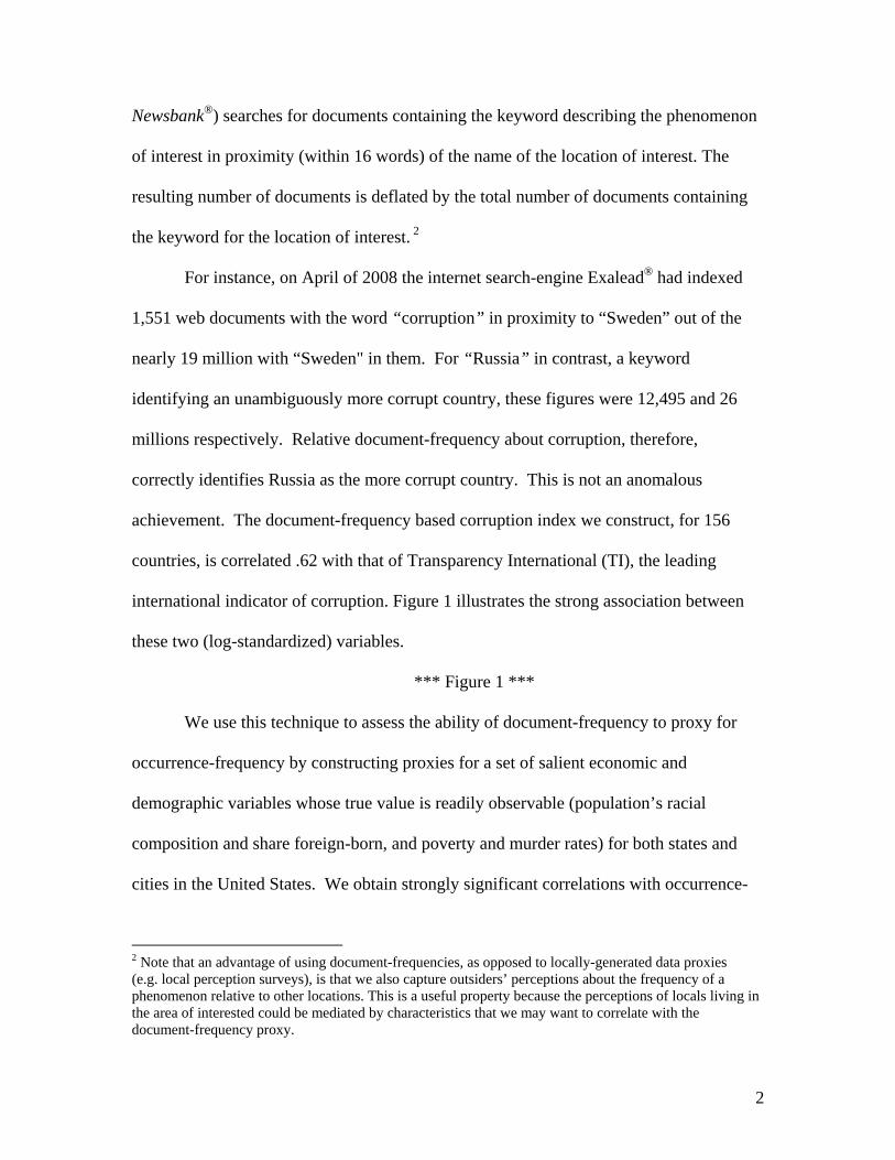
Newsbank®) searches for documents containing the keyword describing the phenomenon

of interest in proximity (within 16 words) of the name of the location of interest. The

resulting number of documents is deflated by the total number of documents containing

the keyword for the location of interest. 2

For instance, on April of 2008 the internet search-engine Exalead® had indexed

1,551 web documents with the word “corruption” in proximity to “Sweden” out of the

nearly 19 million with “Sweden" in them. For “Russia” in contrast, a keyword

identifying an unambiguously more corrupt country, these figures were 12,495 and 26

millions respectively. Relative document-frequency about corruption, therefore,

correctly identifies Russia as the more corrupt country. This is not an anomalous

achievement. The document-frequency based corruption index we construct, for 156

countries, is correlated .62 with that of Transparency International (TI), the leading

international indicator of corruption. Figure 1 illustrates the strong association between

these two (log-standardized) variables.

*** Figure 1 ***

We use this technique to assess the ability of document-frequency to proxy for

occurrence-frequency by constructing proxies for a set of salient economic and

demographic variables whose true value is readily observable (population’s racial

composition and share foreign-born, and poverty and murder rates) for both states and

cities in the United States. We obtain strongly significant correlations with occurrence-

2 Note that an advantage of using document-frequencies, as opposed to locally-generated data proxies (e.g. local perception surveys), is that we also capture outsiders’ perceptions about the frequency of a phenomenon relative to other locations. This is a useful property because the perceptions of locals living in the area of interested could be mediated by characteristics that we may want to correlate with the document-frequency proxy.

3

frequencies: an average correlation of .56 for state-level variables and of .38 for city-level

ones.

Subsequently, we test the usefulness of this technique in a more natural

application: proxying for variables that are not easily observable. We focus on corruption

because it is a difficult-to-measure variable, of interest to economics, and whose variation

can be analyzed at different levels of aggregation (e.g. country, state, and city).

As mentioned above, the document-frequency-based measure of corruption has a

correlation of r = .62 with Transparency International’s corruption perception index. At

the state level the document-frequency proxy is correlated r = .59 with (Edward L.

Glaeser and Raven E. Saks, 2006)’s conviction-based corruption index, and r = .44 with

(Richard T. Boylan and Cheryl X. Long, 2003)’s survey-based one.

Using the document-frequency proxies for corruption as the dependent variable

we replicate the results of (Jakob Svensson, 2005) and (Edward L. Glaeser and Raven E.

Saks, 2006) who establish the correlates of corruption at the country and state level

respectively. Finally, we provide the first city-level index of corruption (for the United

States).

Our research informs a growing literature from various disciplines that attempts to

obtain quantitative information by conducting searches on large databases of documents.

The majority of the existing research has concentrated on making inferences about the

authors of the analyzed text; be it their beliefs (Werner Antweiler and Murray Z. Frank,

2004, Robert Tumarkin and Robert F. Whitelaw, 2001, Peter D. Wiysocki, 1998),

preferences (David Godes and Dina Mayzlin, 2004, Yong Liu, 2006), sentiments (Feng

4

Li, 2006, Paul C. Tetlock, Forthcoming ) or political bias (Matthew Gentzkow and Jesse

M. Shapiro, 2006).

Two exceptions are (Edward L. Glaeser and Claudia Goldin, 2004), who

qualitatively analyzed variation in the number of newspaper articles to discuss major

changes in corruption in the United States during the 20th century, and (Roland G. Jr.

Fryer et al., 2005) who proxied for crack-cocaine availability through time.3

In relation to these literatures we make three notable contributions. First we

demonstrate that analyses of document-frequencies need not be limited to making

inferences about the authors of the written text or about the specific events described in

the text, but more generally, to proxy for the relative frequency of any variable that can

be expressed in frequencies. Second, we advance the conditions under which such

proxying is likely to be valid, aiding future researchers in their decision on whether to use

document-frequencies as proxies, and third, we validate empirically the use of document-

frequency with several demonstrations.

The rest of the paper is organized as follows. Section 2 introduces the conceptual

framework, section 3 contains the empirical analyses of the document-frequency based

proxies for salient economic and demographic variables while section 4 those of

corruption. Section 5 concludes.

2. Conceptual Framework

In this section we lay out a framework establishing the conditions under which

document-frequency is likely to be a valid proxy for occurrence-frequency. We shall

3 Fryer et al. also attempted to capture cross-sectional variation in crack availability but obtained null results. We believe this was the case because their document-frequency data violate two of the data requirements put forward in this paper (data checks #4 and #5).

5

refer to transformations (in a sense specified below) of the occurrence-frequency of

phenomenon p in location l with Yp,l and to the corresponding transformations of the

document-frequency obtained by querying a document database (e.g. the internet) with a

set of keywords k, by klpY ,,ˆ (we utilize subscripts only when needed). We focus on a

linear first-order approximation to characterize the relationship between Y and Y :

(1) klplpkpkpklp YY ,,,,,,,ˆ εβα ++=

where αp,k is a phenomenon-keyword specific intercept, βp,k corresponds to the

impact of the occurrence of phenomenon p, on the number of documents written about it

including keywords k , and εp,l,k to the residual.

Equation (1) is useful for organizing our discussion of various data-checks that

can be performed to assess conditions which make a high correlation between Y and Y

more likely ex-ante. We list all these data-checks in Table 1.

***Table 1***

2.1 αp,k: Maintaining p and k constant.

The most intuitive problem that can arise when attempting to proxy for

occurrence-frequency with document-frequency is α varying across queries; if α is not

constant then β cannot be identified. This means that document-frequency is not useful

for proxying for occurrence-frequency across phenomena.

Different phenomena elicit different levels of overall interest (variation in α from

p) and, in addition, keywords relevant to different phenomena vary in how common it is

for documents about such phenomena to utilize that specific keyword (variation from k).

6

As an example, suppose occurrence-frequency of cause of death by airplane and

car crashes were to be approximated by the document-frequencies for the queries for “car

crash” and “plane crash”. Differences in such document-frequencies could be driven not

only by differences in the occurrence-frequency of such accidents, but also by the

idiosyncratic appeal to write about each of the two causes of death and by the percentage

of all documents about automobile accidents containing the keywords “car crash” vis-à-

vis the percentage of airplane accidents documents containing “plane crash.” This

problem is greatly reduced when comparisons are made across queries that maintain both

p and k constant.

Data check #1: do the different document queries maintain phenomenon and

keywords constant?

2.2 βp,k: frequencies and our basic premise.

Our basic premise, that ceteris paribus the occurrence of a phenomenon increases

the likelihood that a written document about it will be created, is equivalent to assuming

that βp,k>0. Two data checks can be used to assess the validity of this premise. The first

is straightforward: the variable of interest must be expressed in terms of a relative

frequency. The second is that the keyword chosen to search for documents about it is

more likely to be employed following the occurrence than the non-occurrence of the

phenomenon of interest.

The keyword “education” exemplifies violations of both requirements. First,

“education” characterizes a term which does not have a frequency interpretation (unlike,

say, “high-school dropouts”). Second, both an increase and a decrease in the quality of

education in a given location may lead to more documents with the keyword “education.”

7

The second requirement need not rely on subjective judgment alone. It can be

assessed empirically by examining the content of the documents resulting from a given

query. In particular, a researcher can sample the contents of a selection of the documents

found through a particular query and assess whether keyword k is often utilized to

demark the non-occurrence of Y.

Data check #2: is the variable being proxied, Y, a frequency?

Data check #3: Inspect contents of documents found: is the keyword k employed

predominately to discuss the occurrence rather than non-occurrence of

phenomenon p?

2.3 εp,l,k: Efficiency and bias.

εp,l,k captures factors that influence klpY ,,ˆ other than Yp,l . We will discuss here

three such factors: sampling error, measurement error, and violation of the “redundancy-

condition” for proxy variables

(i) Sampling error: Sampling error is reduced as sample size increases, of course,

and hence, considering that document-frequency consists of the ratio of the number of

documents matching the specific query over those about the location overall, sampling

error will play a smaller role for topics and locations where the number of documents is

“large.” In section 3.4 we attempt to estimate what is “large enough” by obtaining

correlations between document-frequency and occurrence-frequency for progressively

larger samples of documents. Our results suggest that an average document-frequency as

small as 50 can be enough to obtain reliable correlations with occurrence-frequency (see

Figure 4).

8

Data check #4: is the average number of documents found large enough for

variation to be driven by factors other than sampling error?

(ii) Measurement error and occurrence variability: for a given amount of

measurement error specific to the relevant keyword and geographic level, a smaller

variance in the occurrence-frequency of the phenomenon will lead to a higher noise-to-

signal ratio and a smaller correlation between occurrence and document-frequency.

To exemplify this problem we proxied for cancer rates across US states and

countries employing document-frequency of “cancer” in proximity to the name of the

location of interest. We expected cancer rates to vary much more across countries than

US states and hence for document-frequency to be a better proxy for the former. Data

from the Center for Disease Control and GLOBOCAN confirmed both expectations. The

coefficient of variation for cancer rates across states is .15 compared to .7 across

countries, and hence the correlation between occurrence and document-frequency was

much higher for variation across countries 0.34 (p<.01) than across states -.06 (n.s.).

Data check #5: is the expected variance in the occurrence-frequency of interest

high enough to overcome the noise associated with document-frequency proxying?

(iii) Measurement error and polysemy: Another possible cause for large

measurement error is that keywords often have multiple meanings, leading to false-

positives; that is, to documents that do contain k but which are not actually about p. To

mute this problem one should replace the keyword for a synonym with fewer other

meanings (for instance using “African Americans” rather than “Blacks”).

9

Data check #6: Inspect content of documents found: does the chosen keyword have

as its primary or only meaning the occurrence of the phenomenon of interest? 4

(iii) Redundancy Condition: The final aspect of ε we discuss deals with its

possible correlation with covariates of Y. This could be a problem if klpY ,,ˆ is estimated to

learn about the relationship between Yp,l and other variables, Xl. A prerequisite for such

use of proxy-variables is that Cov(X, Y |Y)=0 or equivalently that Cov(ε,X)=0 (Jeffrey M.

Wooldrige, 2001). This condition means that, controlling for occurrence-frequency,

document-frequency should be uncorrelated with the covariates of occurrence-frequency.

We consider two possible violations of this condition. The first occurs if X

directly impacts Y , independently of Y. As an example consider Yl =gun ownership in

city l, to be proxied via Y k,l with k=”guns”, and a regression was then to be estimated

with violent crime, X, as a dependent variable (i.e., X=OLS( Y )). If the tendency to write

about guns increases not only as more guns are owned, but also as more guns are used

(e.g. in violent crime), then the correlation between the two will be a biased estimate of

the relationship between gun availability and crime, towards the relationship between gun

use and crime,

4 Fryer et al (2005) computed measures of crack-cocaine availability across cities based on newspaper stories containing the word “crack”, “cocaine” and the name of the city and found no cross-sectional correlation with their 4 other proxies, average correlation: .02 (we thank Roland Freyer for sharing their data). To explore the cause of this null result we conducted (proximity) searches utilizing these keywords and found that for most cities there simply were too few articles to make comparisons across them meaningful. For example, for the year on which most articles appeared, 1989, 45% of all cities had 10 or fewer documents. Variation across cities when the number of documents is so small is likely to be over-ridden by sampling error. We also hand checked the results for one city, Oakland, and found that 80% of the proximity searches were true-positives, compared to 33% of the regular searches, which is what Fryer et al employ. Their data, therefore, violated data-checks #4 and #6.

10

One way to diagnose this problem is to conduct queries that combine keywords

for the occurrence of interest and its covariates (e.g. k=”gun AND murder”); the greater

the share of documents that include the keyword for the covariate, the greater the

potential bias.

If a problem is identified, k can be modified to reduce or eliminate it by, for

example, employing keywords less likely to be used only in association with X. In the

violent example these may include “gun shows” or “gun magazine” instead of simply

“gun” or/and by explicitly requesting the search engine to exclude keywords associated

with X (e.g., using Boolean search to query [(guns NEAR Oakland) NOT murder NOT

crime)].5 Comparisons of the results obtained when such corrections are and are not

implemented should provide guidance of the extent to which Cov( Y ,X|Y)≠0 is driving

the results.

Data check #7: Inspect content of documents found: does the chosen keyword also

result in documents related to the covariates of the occurrence of interest?

The second scenario under which the redundancy condition may be violated is the

presence of an omitted variable, Z, which affects both X and Y independently of Y. For

example, suppose that more cosmopolitan cities foster greater discussion of

socioeconomic issues. Estimates of the correlation between a given covariate X, for

instance average education, and the document-frequency of a given socioeconomic issue

5 NEAR corresponds to a “proximity” search; NOT excludes pages including the specified words. Some illustrative results: the query for “gun” on January 19th, 2007 lead to 29.1 million hits on Exalead, of which 3.3 million, or 11%, also contain the words murder, murders or murdered. In contrast, of the 155,744 documents for “gun show” only 4,720, or 3%, contained such words.

11

like “poverty” ( Y ) will be biased towards the relationship between average education and

cosmopolitanism (Z). i.e. Cov( Y ,X) will be biased towards Cov(Z, X).

To fix this problem additional searches can be conducted to proxy either for the

underlying omitted variable (e.g. “cosmopolitan”) or for the suspected latent variable

influenced by the omitted one (e.g. “socioeconomic”) and assess the impact of controlling

for this additional document frequency on the parameter estimates of interest.

Data check #8: are there plausible omitted variables that may be correlated both

with the document-frequency of the variable of interest and its covariates? If so,

control for the omitted variable with an additional document-frequency proxy.

3. Demonstrations with observable occurrence-frequencies

We begin the empirical analyses with a few demonstrations of how document-

frequency can be used to proxy for occurrence-frequency. We conducted our document-

frequency estimations both on the internet, using the search engine Exalead, 6 and on the

local newspaper database Newsbank. 7 We focus on contemporaneous web searches and

on newspapers published in the five years between 9/1/2001 and 31/8/2006, because the

Newsbank’s coverage is very limited before the initial date.

To conduct this initial demonstration we selected variables capturing salient

socioeconomic dimensions and readily available at the state and city level. In particular,

we constructed proxies for share of the population that is African-American, Hispanic,

and foreign born, and for both murder and poverty rates. 6 At the time of our data-collection, only Exalead provided the option of conducting proximity searches, using 16-word textual distances 7 We considered two other newspaper databases: Lexis-Nexis and Factiva. We chose Newsbank because it has the largest set of local newspapers and because, unlike Lexis-Nexis, it does not place a limit on the number of documents found on a single query. We queried both Newsbank and Exalead utilizing specially designed PERL scripts. Importantly, we added considerable time delays between queries to avoid imposing unreasonable burdens on the servers.

12

We obtained occurrence-frequency data for these variables from aggregate census

counts, the FBI’s Uniform Crime Reports, and HUD State of the Cities Database,

respectively. For state level poverty we use the percentage of population with income

below one half of the state median. For poverty at the city level we do not have microdata

for all the cities so we use instead the official poverty rate as reported by the census. 8

To estimate document-frequency we conducted proximity searches with the

keywords “African American OR African Americans,” “Hispanic OR Hispanics,”

“Immigrant OR Immigrants,” “poverty,” and “murder.” We used all cities with a

population of 100,000 or more in the 2000 census and all 50 states as locations. We

excluded cities that have the same name as another city of more than 100,000 inhabitants,

such as Arlington and Springfield.

As mentioned above, we calculate document-frequency as the ratio of documents

obtained via a proximity search and the total number of documents with the name of the

location. The distributions of both occurrence and document-frequencies tend to have a

right skew, and we conduct all analyses on the log of these variables.9 Figure 2 shows the

occurrence and document-frequency distributions of the share of African-Americans

across cities and their log-standardized version. The graphs also display the normal

distribution that has the mean and variance corresponding to the data.

***Figure 2***

To assess the validity of this transformation we estimated the parameter λ in

Box-Cox regressions of the general form:

8 Note that these poverty rates are computed utilizing a nation-wide nominal income threshold, overestimating poverty in cheaper cities and underestimating it for expensive ones. This measurement error induces a conservative bias in our estimated correlations. 9 We add 1 to the numerator so that the few cases with 0 documents can be included in the analyses..

13

(2) klplp

kpkpklp YY

,,,

,,,, 1)(1)ˆ(

ελ

βαλ

λλ

+−

+=−

Where, again, Y k,p,l is the relative document-frequency of occurrence p with

regards to location l as proxied by keyword k and Yp,l is the corresponding occurrence-

frequency. The estimate of λ indicates the optimal Box-Cox transformation to both

variables. λ = 0 indicates a log transformation.

We fitted the Box-Cox model for our 5 keywords, both for the internet and

newspapers, both at the city and state level. The average of the resulting 20 estimates of λ

was M = -0.107, SE = 0.037. While this is statistically significantly different from zero

it is quite close to it. Indeed, 12 of the 20 point estimates are not statistically different

from 0. Furthermore, the log transformations are very highly correlated with those

resulting from using the λs from the Box-Cox transformation,

3.1 Data checks

Before conducting the analyses we examine whether the variables of interest pass

the data-checks put forward in our framework. They of course pass checks #1 (keywords

are kept constant across locations), and # 2 (occurrence of the phenomena can be

expressed in relative frequency terms).

For data-check #3 (keyword is more commonly used for occurrence rather than

non-occurrence of phenomenon) and #6 (keyword’s primary meaning is that of the

phenomenon of interest) we conducted searches for each of the keywords in proximity to

the word “city” and examined the contents of the first 50 documents found. For “African

American” and “Immigrants” all 50 documents were true positives (e.g. Cleveland’s

14

African American Museum and the Coalition for Humane Immigrant Rights in Los

Angeles). For “Hispanics” and “Poverty” 49 out of 50 were true positives. For murder,

in contrast, only 14 out 50 pages made direct allusion to actual murder cases or murder

rates many documents referred to murder mystery clubs, TV shows, or pop songs. In the

pool of 250 documents sampled, no document made allusion to any of the keywords to

signify absence or reduced occurrence of the phenomena (e.g. “no immigrants” or “lack

of poverty,” “less Hispanics,” or similar). Data-check #3 hence passes all keywords,

while data-check #6 does too with the exception of “murder.”

Data-check #4 requires raw document-frequency to be high enough that variation

in relative frequencies across locations can have a reasonable signal to noise ratio. In our

data, the average number of internet documents found for a given keyword ranged

between 410 (for “corruption” at the city level) and 35,957 (for “African Americans” at

the state level; both number are much higher than what our calibrations in section 3.4

suggest are sufficient for obtaining valid proxies.10

Data-check #5, requiring occurrence-frequency to experience substantial

variation, will typically consist of a qualitative a-priori assessment. For the variables in

this demonstration, however, we can directly assess the variation in occurrence-frequency

since we are proxying for observable variables. In Table A2 in the Appendix we provide

summary statistics for all the variables being proxied. The coefficients of variation are

relatively high across the board, hovering around 75%-110%. Poverty is the notable

exception, with a coefficient of variation of just 9% at the state level, for example. We

should expect, therefore, that poverty’s document-frequency will be less strongly

10 See Table A1 in the appendix for a full list of the number of documents found for each keyword at different levels of analysis. For newspapers the range is between 97 for “corruption” at the city level and 3,085 for “murder” at the state level.

15

correlated with its occurrence-frequency. Finally, data-checks #7 and #8 do not apply

here since we are not estimating regressions.

In sum, we expected positive correlations between occurrence and document-

frequency for the social phenomena under consideration. The data-checks, however,

suggest that we should encounter weaker correlations for murder with its high rate of

false-positives, and for poverty with its low occurrence-frequency variation.

3.2 Results

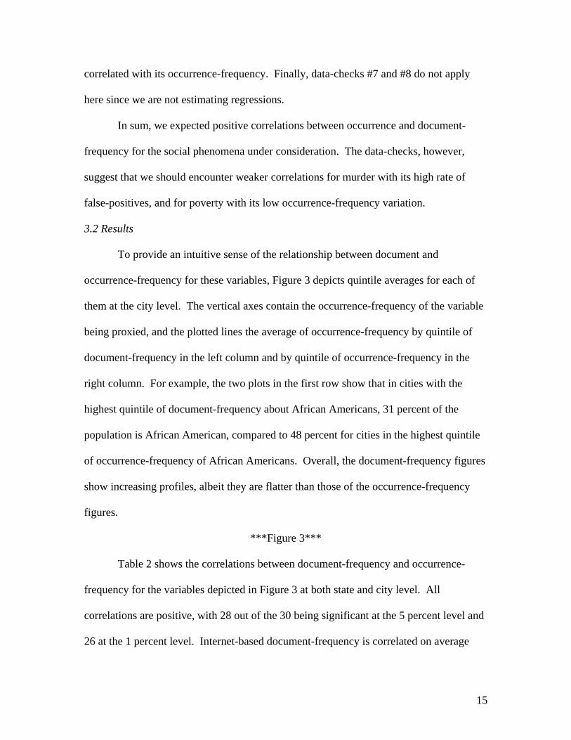
To provide an intuitive sense of the relationship between document and

occurrence-frequency for these variables, Figure 3 depicts quintile averages for each of

them at the city level. The vertical axes contain the occurrence-frequency of the variable

being proxied, and the plotted lines the average of occurrence-frequency by quintile of

document-frequency in the left column and by quintile of occurrence-frequency in the

right column. For example, the two plots in the first row show that in cities with the

highest quintile of document-frequency about African Americans, 31 percent of the

population is African American, compared to 48 percent for cities in the highest quintile

of occurrence-frequency of African Americans. Overall, the document-frequency figures

show increasing profiles, albeit they are flatter than those of the occurrence-frequency

figures.

***Figure 3***

Table 2 shows the correlations between document-frequency and occurrence-

frequency for the variables depicted in Figure 3 at both state and city level. All

correlations are positive, with 28 out of the 30 being significant at the 5 percent level and

26 at the 1 percent level. Internet-based document-frequency is correlated on average

16

.439 with occurrence-frequency, almost identical to the correlation between newspaper-

based document-frequency and occurrence-frequency, .440.11

***Table 2***

We interpret the positive correlations between document and occurrence-

frequency as supportive of our contention that, for data that pass the multiple data-

checks, greater occurrence-frequency of a specific phenomenon is associated with

increased document-frequency of that same phenomenon.

Considering that the five variables we proxied are related to socio-economic

status it is possible that rather than five independent demonstrations, the above

correlations capture the same correlation between document-frequency and occurrence-

frequency of low socioeconomic status, five times.

A more troubling concern is that this single correlation could be spurious. This

could occur if people living in cities with greater frequency of low socioeconomic status

were interested in writing about socioeconomic issues for reasons other than a high local

occurrence-frequency per-se. For example, one may worry that large numbers of

documents are written about African Americans in Philadelphia not because of

Philadelphia’s large African American community, but because of Philadelphia’s large

Democratic Party voter base, say, which will tend to discuss all socioeconomic issues,

including those pertinent to the African American community.

We address these concerns in Table 3, where we report the cross-correlations of

document-frequency and occurrence-frequency of African-Americans, with the

occurrence-frequency of all five demographic variables used in the above

11 Table 1 reports Pearson correlations. Unreported Spearman correlations (based on rank and therefore not sensitive to outliers or log-standardization) were very similar. The averages across all variables are .47 for Newspapers and .45 for the Internet.

17

demonstration.12 Contrary to the null hypothesis that there is a single latent variable

driving all correlations in Table 2, several of the cross-correlations between African

American document-frequency and the occurrence-frequency of other variables are

negative, and –importantly- similar to the cross-correlations in occurrence-frequency.

For example, the cross-correlation between the occurrence-frequency of Hispanics and

the document-frequency of African-Americans is -.40 across cities, compared to an actual

correlation between both occurrence-frequencies of -.54.

***Table 3***

An alternative way to address this concern, suggested in the conceptual

framework, consists of controlling the suspected omitted variable also with an additional

document-frequency proxy. Importantly, this approach can easily be applied in situations

where, unlike the present example, actual occurrence-frequencies are not observable.

If a single latent variable accounts for the multiple correlations we obtain, then

partialing out the variance contained in a proxy of such a variable should substantially

mute the (spurious) correlations. Because we are concerned with an overall tendency to

discuss socioeconomic issues, we estimated the relative document-frequency of the

keyword “socioeconomic.” If the correlations from Table 2 arise because of a spurious

association between the occurrence-frequency of those variables with the tendency to

discuss socioeconomic issues, this variable should help us capture this trend and weaken

the obtained correlations. Contrary to this prediction, we find that controlling for relative

frequency of “socioeconomic” leaves the correlations between document-frequency and

12 We focus on the African-American share because this is the variable for which document-frequency is more strongly correlated with occurrence-frequency and therefore where we have more power. Considering that we are seeking to show lack of correlation across variables this is the most conservative test we can take. We focus on states and major cities for analogous reasons.

18

occurrence-frequency from Table 2 largely unchanged: .41 on average for states, .38 for

cities, and .44 for large cities, compared to .52, .38 and .42 respectively.

3.3 Monotonicity

We have established that document frequencies are strongly correlated with

occurrence frequencies on average. Here we examine whether the relationship between

the two is monotonic. This would not be the case if, for instance, at very high or low

levels of occurrence changes in empirical frequencies were negatively related to changes

in publication frequencies at the margin.

To examine this issue we pooled observations from all variables at the city level

and estimated a spline regression. We identified cutoff points for quintiles of occurrence-

frequency (of all variables pooled) and then each observation’s occurrence-frequency was

compared to these ’knots’.

In particular, let the new five spline variables be represented by Si with i=1 to 5,

and the inter-quintile cutoff point separating quintile i from quintile i+1 be represented

by ki.

The value of Si is determined by the following conditions:

If y < ki then Si = 0

If ki≤ y ≤ ki+1 then Si = y - ki

If y > ki+1 then Si = ki+1 - ki

Note that y = S1+S2+S3+S4+S5.

A regression with document-frequency as the dependent variable and S1 through

S5 as predictors estimates the marginal impact of occurrence-frequency on document-

19

frequency separately for variation in occurrence-frequency happening in each of its five

quintiles.

Considering that we pooled observations across all phenomena we include slope

dummy interactions for them (e.g., a “murder” dummy interacted by occurrence-

frequency).13 Table 4 shows the results for both internet and newspaper based document-

frequencies. All point estimates are positive, and with a few exceptions significant,

indicating that within each quintile of occurrence-frequency, a marginal increase in

occurrence-frequency is associated with an increase in document-frequency in the

margin.

***Table 4***

3.4 Reliability and sample size

As mentioned in our discussion of data check #4, if the absolute document-

frequencies are small, variation across locations will be overridden by sampling error and

hence the resulting proxy will be unreliable. In this subsection we gauge the relationship

between sample size and the strength of the measured correlations

The ideal way to do so would be to query the full databases of documents we use

(Newsbank® and Exalead®) and to create random subsamples of varying sizes from the

resulting sets of documents. This approach, unfortunately, is prohibitively costly, as it

requires downloading and analyzing the millions of documents that are obtained with the

queries (e.g., just with “New York” there are over 60 million web documents).

As an alternative, we conducted queries on the full universe of documents but

restricting searches so that only documents published during shorter periods of time

13 Main effect dummies are not included because the variables were standardized separately. African-American share is the excluded interaction.

20

would be considered. We focus on newspaper data at the city level using Newsbank®. In

particular, rather than conducting a single query per location-variable pair for all

documents published between 2001 and 2006, we conducted 60 such queries per

location-variable pair (e.g. “crime” NEAR “Los Angeles”), restricting the results to have

been published during each of the 60 months.14 The resulting document-frequencies are

hence based, on average, on samples 1/60 the size of the original sample. By adding up

partial sums for different (randomly selected) months we can then create larger samples.

We assess the impact of increasing average absolute number of documents by

monitoring the evolution of the correlation between actual occurrence-frequency and

document-frequencies computed over samples of increasingly larger sizes.15

Figure 4 shows the results from this exercise conducted on two different random

subsets (without replacement) of 30 months each. The x-axis contains the average

number of documents in the cumulative sample, as more and more months are added in

random order, and the Y-axis the correlation of the proxy arising from that sample with

the corresponding occurrence-frequency. Random sample 1 is plotted with dark points,

whereas sample 2 is pictured using transparent diamond signs.

***Figure 4***

The results depicted in Figure 4 are highly comparable for the two random

subsamples we employed (which have no overlap). They suggest that an average number

of documents as low as 50 can generate valuable proxies for occurrence-frequency, and

14 We conduct these searches only on Newsbank because internet searches with date restrictions, although possible, are not very reliable. Most notably, they obviously do not retrieve documents that were uploaded in the past but which are no longer available. 15 The fact that we are sampling at the month level rather than independently at the document level reduces the efficiency of our samples. Truly random subsamples should converge faster, leading to an even smaller number of documents required to achieve a robust proxy.

21

that increasing average number of documents above 200 no longer noticeably increases

accuracy.

4. Document-frequency based measures of corruption.

The results from the previous section demonstrated that document-frequency can

be significantly correlated with occurrence-frequency. In this section we examine

whether such correlation can be exploited to construct proxies for unobservable variables,

which can then be used to learn about the covariates of the variable of interest.

We focus on corruption for two main reasons. First, doing so reduces possible

concerns of data snooping to a minimum. Because published papers have studied

correlates of corruption both at the state and country level, by concentrating on corruption

we require the exact same technique to replicate prior findings in settings with

independent sources of variation.

Second, the study of corruption characterizes the ideal application for the

quantification of document-frequency: approximating the occurrence-frequency of a

phenomenon that is otherwise very expensive to measure. Transparency International’s

Corruption Perceptions Index (CPI), the most commonly used international measure,

averages information from 16 different surveys on experts and businessmen, some of

them containing responses from more than 4,000 individuals. The high costs associated

with data collection on corruption not only lead to large expenses, but also to censored,

incomplete, or even nonexistent data sets. The International Crime Victim Survey from

the year 2000, for example, which includes questions about bribes, was administered in

only 48 countries. Quantifying document-frequency, in contrast, is virtually free and can

in principle be conducted at any level of aggregation.

22

We present results using both internet and newspaper document-frequency, but

center our discussion on the internet measures: these always work as well, if not better,

than newspaper-based variables, are more widely available, and reflect documents from a

much more diversified set of social agents.

4.1 Country-level variation

We start by analyzing corruption at the country level. We conducted searches for

“corruption” in proximity to the name of 154 countries, deflating the resulting number of

documents by the number obtained searching only the countries’ names. The resulting

correlation between occurrence and document frequencies is positive and significant:

0.62 (see figure 1 for a plot chart).

An important question is the extent to which the documents we are finding are

actually discussing Transparency International’s CPI. On the one hand that would be

good news for the validity of the technique, as it would demonstrate its ability to capture

relevant information. On the other it would be bad news if document-frequency works

solely because it relies on existing occurrence-frequency estimates readily available

online. We addressed this issue by conducting a new search adding a restriction that

excluded all documents containing the word “transparency,” presumably leaving out an

important share of documents that discuss corruption in relation to the CPI.16 If

document-frequency was mostly picking up variation created by the CPI, then the new

index should be much less closely correlated with the CPI. The new correlation,

however, is virtually identical: .60.

16 The queries were of the following general form: ((corruption NEAR <country>) NOT transparency)).

23

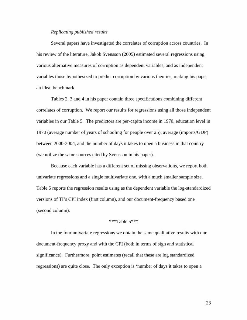
Replicating published results

Several papers have investigated the correlates of corruption across countries. In

his review of the literature, Jakob Svensson (2005) estimated several regressions using

various alternative measures of corruption as dependent variables, and as independent

variables those hypothesized to predict corruption by various theories, making his paper

an ideal benchmark.

Tables 2, 3 and 4 in his paper contain three specifications combining different

correlates of corruption. We report our results for regressions using all those independent

variables in our Table 5. The predictors are per-capita income in 1970, education level in

1970 (average number of years of schooling for people over 25), average (imports/GDP)

between 2000-2004, and the number of days it takes to open a business in that country

(we utilize the same sources cited by Svensson in his paper).

Because each variable has a different set of missing observations, we report both

univariate regressions and a single multivariate one, with a much smaller sample size.

Table 5 reports the regression results using as the dependent variable the log-standardized

versions of TI’s CPI index (first column), and our document-frequency based one

(second column).

***Table 5***

In the four univariate regressions we obtain the same qualitative results with our

document-frequency proxy and with the CPI (both in terms of sign and statistical

significance). Furthermore, point estimates (recall that these are log standardized

regressions) are quite close. The only exception is ‘number of days it takes to open a

24

business,’ where the document-frequency point estimate is less than half that obtained

with Transparency International’s CPI.

The lower panel in Table 5 shows the results combining all four predictors into a

single regression. Comparing both columns the general pattern is the same: document-

frequency obtains results very similar to those obtained with the CPI, with the exception

of the number of days to open a business. The results from Table 5 indicate that one can

learn almost the same about the correlates of international corruption by either

conducting expensive surveys of thousands of individuals or by running a few hundred

searches on the internet, which takes a matter of hours.

4.2 State level variation

We next turn our attention to corruption across states in the United States. Unlike

the case of corruption across countries, no widespread index of corruption exists for

different states. We are aware of two assessments of state level corruption; we used both

as benchmarks for our document-frequency based index of state corruption.

The first consists of a survey conducted by (Richard T. Boylan and Cheryl X.

Long, 2003). They provided a questionnaire to 834 state house reporters, obtaining 293

responses (from 45 different states). They constructed their corruption index with the

average of some of the questions in their questionnaire.

The second assessment of corruption across states is that of (Edward L. Glaeser

and Raven E. Saks, 2006), referred to as GS for the remainder of the paper. They

constructed a state-level corruption index based on the number of government officials

convicted for corrupt practices through the (federal) Department of Justice (DOJ). In

25

particular they divided the average number of DOJ corruption convictions over the 1976-

2002 period by the state’s average population during that same period.17

As GS acknowledge, there is a problem with deflating convictions by population,

as doing so assumes that the number of government officials that could be corrupt has a

linear relationship with population. States, of course, differ in the proportion of their

citizens working for the government and hence at risk of engaging in the kind of behavior

which could lead to a federal conviction. With this consideration in mind, and

particularly because size of government is one of the predictors used by GS, we use in

addition to the index published in their paper, one which deflates DOJ convictions by the

average number of government employees during 1976-2002.18

Altogether we have 5 measures of corruption at the state level: (i) the original

GS index, (ii) GS computed deflating by number of public employees rather than

population for 1976-2002 (iii) Boylan and Long (2003)’s survey, (iv) internet based

document-frequency index, and (v) newspaper based document-frequency index. In

order to compare these variables measured in different units, as was done in the previous

sections, we log-standardize all indexes.

Figure 5 depicts the relationship between measures (ii) and (iv). Corruption

measured by average convictions per public employee during the 1976-2002 period

appears in the vertical axis and document-frequency of corruption on the internet on the

x-axis. The graph shows an obvious association between both measures of corruption.

17 Corporate Crime Reporter, http://www.corporatecrimereporter.com/corruptreport.pdf, constructs essentially the same index. 18 Glaser and Saks (2006) point out that their preferred deflator would have been the number of public officials by state, for which data are not available. Number of public employees, however, is available. We suspect it is more highly correlated with number of officials than state population is.

26

The correlations among all indexes are presented on Table 6. The average

correlation between the internet measure and the three occurrence-frequency based

measures is .49 (column 1). Interestingly, internet document-frequency is more highly

correlated with the DOJ and survey-based indexes than they are with each other

(although the difference is not significant at conventional levels).

***Table 6 ***

When convictions are divided by public employees rather than population, the

correlations with other corruption measures increase (e.g. from .43 to .59 with internet

document-frequency and from .31 to .41 with Boylan & Lang (2003)’s survey. This is

consistent with our claim that number of public employees is a more appropriate

denominator for corruption convictions.

We now move to replicating previous corruption research at the state level. We

estimate regressions with our various corruption measures as dependent variables and the

same predictors used in GS table 4, column 1, as independent variables: income

inequality (Gini in 1970), median income (in 1970), education (share of population with

college degree in 1970), share of employment provided by the government, (log of)

population size, share of population living in an urban area, and regional dummies. This

specification nests all previous ones in GS.19

The results are reported in our Table 7. Column 1 uses the original GS measure,

column 2 the alternative version deflated by number of public employees, column 3 an

19 Most of the data for the predictors used in the regressions for Table 7 were kindly provided by Raven Saks.

27

internet based document-frequency index, column 4 the survey and column 5 the

newspaper based document-frequency.20

***Table 7 ***

Comparing columns 1 and 2, we see that deflating convictions by number of

public employees rather than population increases the size of most coefficients,

maintaining significance mostly unchanged (consistent with the notion that such deflator

reduces measurement error). The notable exception is, not surprisingly, the estimated

impact of share of government employees, which drops to less than 5 percent of its

original size and is no longer significant.

Most importantly, column 3 shows that, using our internet document-frequency

measure of corruption as an independent variable, we obtain results that are largely

consistent with those from columns 2 and 1. Greater income inequality, greater income

levels and lower education are all associated with an increase in the internet corruption

index in this specification. The point estimates are of similar magnitudes across the three

columns, although education is slightly less important in the document-frequency

regression. The biggest difference across columns occurs with the impact of share of

20 In Table 5 we exclude from the analyses the state of Georgia, because (contrary to our data-check 6) most documents allude to the Caucasian country and not to the US state of interest: for example, 34 out of the 50 first pages containing the keyword “corruption” and “Georgia” allude to the ex-Soviet Union country. We also exclude Washington State, since a majority of web pages alluding to Washington are actually in relation to the District of Columbia. 28 out of the 50 first pages containing the keyword “corruption” and “Washington State” allude to the US capital: if included in the sample Washington State would be a huge outlier, with internet frequencies two and a half standard deviations above the mean and occurrence-frequencies two standard deviations below the mean. While becoming slightly more imprecise, our main results are actually robust to the inclusion of these two states: the coefficients (standard errors in parentheses) on inequality, income, and percentage with bachelors degree become 0.68 (.28), 0.62 (.27), and -0.31 (.16)

28

employment provided by the government. It is estimated as small positive and non-

significant in column 2 and negative and significant in column 3.21

The results obtained with the survey of house state reporters, column 4, are not

dissimilar qualitatively, but many of the parameter estimates are not significantly

different from zero. Our internet document-frequency-based proxy, hence, appears to be a

better measure of corruption, in this case, than costly survey data.

Throughout their paper, GS show numerous others regressions studying the

relationship between corruption and a variety of additional variables, controlling for all

variables included in Table 7 except income inequality. In our Table 8 we report the

results from replicating the subset of these additional regressions which GS find to have a

significant relationship with corruption (at the 5% level). Some of the estimates using the

log version of GS’s measure are no longer significant, but point estimates for the

occurrence-frequency and document-frequency based measures of corruption are

remarkably similar.

***Table 8 ***

In sum, we construct a measure of corruption which is both highly correlated with

the two existing measures of state level corruption, and which we use to replicate the

findings from existing research assessing the correlates of corruption at the state level.

4.3 City- level variation

We now turn to using document-frequencies to produce the first assessment of

corruption at the city level in the US. Document-frequency-based proxies have an

21 To assess whether we capture variation in corruption in addition to that which is captured by the predictors employed by GS, we estimated a regression equivalent to Column 2 in Table 5 adding internet document-frequency as a predictor. We obtained a positive and significant point estimate (t-stat = 2.66).

29

important component of error. Considering that previous research has shown that readers

of rankings tend to overweight positional differences over differences in the underlying

continuous variables that are used to construct these rankings (Devin G. Pope, 2006), we

present the results from our estimation of corruption at the city level in groups of 10

cities. The results for the 61 cities with more than 250,000 inhabitants are presented in

Table 9. The top-10 cities are consistent with our priors on corruption, including San

Diego, New Orleans, Los Angeles, Philadelphia, and Chicago. Conversely, among the

bottom-10 we find cities seldom used as examples of corrupt local governments.22

***Table 9 ***

To complement this subjective assessment of the city-corruption index, we also

estimated regressions employing it as a dependent variable. Unfortunately, we are unable

to exactly replicate the state-level or country-level specifications because some covariates

at greater level of aggregation are either unavailable for cities (e.g. income inequality) or

lack variation (e.g. percentage of the population living in cities). In order to obtain a

benchmark from existing measures of corruption, therefore, we estimate a new state-level

regression with the same covariates employed for the city-level regressions.

The results are presented on Table 10. In all columns except 2 & 3 the dependent

variable is city-level corruption as proxied by internet document-frequency. In column 2

it is city-level corruption as proxied by Newspaper document-frequency and in column 3

state level corruption as measured by DOJ corruption convictions per public employee.

***Table 10***

22 In line with data check #6, we dropped cities whose names are more often used to mean something other than the city in question. In particular we dropped Independence, Washington, Toledo, and Athens. “Toledo,” for instance, is much more commonly used to refer to the former Peruvian president than to the city in connection to corruption. For example, in January of 2007, of the first 10 hits for “Corruption NEAR Toledo” in Exalead, nine discussed the former president and only one the Ohioan city.

30

The results across columns 1,2 and 3, i.e. for variation across cities and sates,

are similar in qualitative terms, lending credence to the city level corruption measures we

have created. In particular, city and state level regressions indicate that locations with

greater income, smaller populations, and fewer minorities and immigrants have less

corruption. The main difference in point estimates is the South dummy, which is positive

at the state level (indicating greater state corruption in the South than in the omitted

region, the west) but is negative in the city level regression.

One of the benefits of obtaining city level data is the possibility of studying

covariates that vary at a finer level of aggregation than at the state level. As an example

we examine if industrial cities tend to experience more corruption (possibly as a

consequence of their recent economic downturn). To this end we add as a predictor of

city-level corruption the share of employment in the manufacturing sector, which proves

–surprisingly- negatively associated with corruption (see column 4).

We next examine two possible concerns regarding our city-level analyses of

corruption. The first is the possibility that variation in our corruption proxy is driven not

by variation in the occurrence-frequency of corruption across different cities, but rather,

by variation in the tendency to write about social issues in relation to different cities. For

example, we find that larger cities (in population) tend to be measured as more corrupt,

the concern is that this correlation may result from people being more inclined to writing

about social issues with regards to larger cities.

As suggested in our discussion of such problem in data-check #8, we assess the

potential importance of this concern by estimating the document-frequency of a variable

that may proxy for the omitted variable in question. We use again the document-

31

frequency of the keyword “socioeconomic” and add this variable as a control in

column 5. Although it proves a significant predictor of the document-frequency of

corruption, the point estimates for the other variables remain largely unchanged,

suggesting omitted variables of the kind we considered are not a problem in the original

specification.

The second concern we address is the possibility that our city-level regression

results capitalize on state-level variation in corruption. To address this concern in

column 6 we control for our state-level document-frequency based measure of corruption.

We find that (i) state-level document-frequency of corruption is not a significant

predictor of city-level corruption (controlling for city observables), and (ii) that more

importantly, its introduction in the model does not greatly influence the point estimates of

the other independent variables.23 This strongly suggests we are capturing variation in

corruption above and beyond state-level corruption.

In sum, our document-frequency measure of corruption at the city level both

generates a ranking of cities that is consistent with our preconceptions and with findings

about the covariates of corruption at greater levels of aggregation.

6. Conclusions

We hypothesized that, ceteris paribus, the occurrence of a social phenomenon

increases the chances people will publish content about it. In this paper we have

demonstrated that using variation in relative measures of internet and newspaper

document-frequency in reference to a phenomenon can capture cross-sectional variation

of the underlying corresponding empirical occurrence-frequencies.

23 Results are almost identical if, as in Table 5, we exclude Georgia from the regression (3 cities).

32

We begun by introducing a framework that specified the circumstances under

which the frequency of documents containing specific keywords in relation to a given

location (e.g. a country, state, or city) might be used as a proxy for the occurrence-

frequency of the discussed social phenomenon. We then validated the technique showing

strong, positive, statistically significant correlations between document-frequency and

empirical data on several major demographic variables.

Focusing on the measurement of corruption at the country, state and city level we

also found that document-frequency based measures of corruption were highly correlated

with published measures of corruption. Regression analyses utilizing the document-

frequency based measures of corruption for countries and states replicated the sign,

significance and magnitude of the covariates of corruption from published papers.

Strikingly, using data that we obtained from the internet and newspaper databases in a

matter of hours, we obtain results similar to those arising from data based on expensive

surveys or administrative collection processes, illustrating the simplicity and potential

power of this approach.

Our results demonstrate that when the requirements put forward in the framework

are met, document-frequency’s correlation with occurrence-frequency allows researchers

to construct proxies for otherwise unobservable variables. This opens the door to

studying previously not-measured variables, as we do here with city-level corruption. A

promising application is the possibility of creating proxies for suspected omitted

variables in settings where the dependent variable is observable, an exciting possibility

considering that a large number non-experimental field studies suffer from potential bias

due to omitted variables.

33

References Alesina, Alberto; Baquir, Reza and Easterly, William. "Redistributive Public Employment." Journal of Urban Economics, 2002, 48, pp. 219-41. Antweiler, Werner and Frank, Murray Z. "Is All That Talk Just Noise? The Information Content of Internet Stock Message Boards." The Journal of Finance, 2004, LIX(3), pp. 1259-94. Boylan, Richard T. and Long, Cheryl X. "A Survey of State House Reporters’ Perception of Public Corruption." State Politics and Policy Quarterly, 2003, 3(4), pp. 420-38. Clemen, Robert T. "Combining Forecasts: A Review and Annotated Bibliography." International Journal of Forecasting, 1989, 5, pp. 559-83. Fryer, Roland G. Jr.; Heaton, Paul S.; Levitt, Steven D. and Murphy, Kevin M. "Measuring Crack Cocaine and Its Impact," NBER Working Paper. 2005. Gentzkow, Matthew and Shapiro, Jesse M. "What Drives Media Slant? Evidence from U.S. Daily Newspapers," NBER Working Paper. 2006. Glaeser, Edward L. and Goldin, Claudia. "Corruption and Reform: An Introduction," NBER Working Paper. 2004. Glaeser, Edward L. and Saks, Raven E. "Corruption in America." Journal of Public Economics, 2006, 90(6-7), pp. 1053-72. Godes, David and Mayzlin, Dina. "Using Online Conversations to Study Word-of-Mouth Communication." Marketing Science, 2004, 23(4), pp. 545-60. Li, Feng. "Do Stock Market Investors Understand the Risk Sentiment of Corporate Annual Reports?," Available at SSRN: http://ssrn.com/abstract=898181 2006. Liu, Yong. "Word of Mouth for Movies: Its Dynamics and Impact on Box Office Revenue." Journal of Marketing, 2006, 70, pp. 74-89. Mauro, Paulo. "Corruption and Growth." Quarterly Journal of Economics, 1995, 110(August), pp. 681-712. Pope, Devin G. "Reacting to Rankings: Evidence From "America's Best Hospitals and Colleges"," Job Market Paper, University of California-Berkeley, Economics Department. 2006. Svensson, Jakob. "Eight Questions About Corruption." Journal of Economic Perspectives, 2005, 19(3), pp. 19-42. Tetlock, Paul C. "Giving Content to Investor Sentiment: The Role of Media in the Stock Market." The Journal of Finance, Forthcoming. Tumarkin, Robert and Whitelaw, Robert F. "News or Noise? Internet Message Board Activity and Stock Prices." Financial Analysts Journal, 2001, 57(3), pp. 41-51. Wiysocki, Peter D. "Cheap Talk on the Web: The Determinants of Postings on Stock Message Boards," University of Michigan Business School Working Paper. 1998. Wolfers, Justin and Zitzewitz, Eric. "Prediction Markets." Journal of Economic Perspectives, 2004, 18(2), pp. 107-26. Wooldrige, Jeffrey M. Econometric Analysis of Cross Section and Panel Data. Cambridge: MIT Press, 2001.

Figure 1: Corruption in the World

AfghanistanAlbania

Algeria

Angola

ArgentinaArmenia

AustraliaAustria

Azerbaijan

Bahrain

Bangladesh

Barbados

Belarus

Belgium

Belize

Benin

Bolivia

Bosnia+and+Herzegovina

Botswana

BrazilBulgaria

Burkina+Faso

Burundi CambodiaCameroon

Canada

Chad

Chile

China

ColombiaCosta+Rica

Croatia

Cuba

Cyprus

Czech+Republic

Denmark

Dominican+Republic

Ecuador

Egypt

El+Salvador

Equatorial+Guinea

Eritrea

Estonia

Ethiopia

Fiji

Finland

France

GabonGambia

Georgia

Germany

Ghana

Greece

GuatemalaGuyana

Haiti

Honduras

Hong+Kong

Hungary

Iceland

India

Indonesia

Iran

Iraq

Ireland

Israel

Italy

Jamaica

Japan

Jordan

Kazakhstan

Kenya

Kuwait

Kyrgyzstan

Laos

Latvia

Lebanon

Lesotho

Liberia

Libya

Lithuania

Luxembourg

MacedoniaMadagascar Malawi

Malaysia

Mali

Malta

Mauritius

Mexico

MoldovaMongolia

Morocco

Mozambique

Myanmar

Namibia

Nepal

Netherlands

New+Zealand

NicaraguaNiger

Nigeria

Norway

Oman

Pakistan

Palestine

Panama

Papua+New+Guinea

Paraguay

Peru

Philippines

Poland

Portugal

Qatar

Romania

Russia

Rwanda

Saudi+ArabiaSenegal

Serbia

Seychelles

Sierra+Leone

Singapore

Slovakia

Slovenia

Somalia

South+Africa

South+Korea

Spain

Sri+Lanka

Sudan

Suriname

Swaziland

SwedenSwitzerland

Syria

Taiwan

Tajikistan

Tanzania

ThailandTrinidad+and+Tobago

Tunisia

Turkey

Turkmenistan

UgandaUkraine

United+Arab+Emirates

United+Kingdom

United+States

Uruguay

UzbekistanVenezuela

VietnamYemen

Zambia Zimbabwe

-2-1

01

2T

ranspa

rency In

tern

atio

na

l C

PI

-3 -2 -1 0 1 2Corruption internet document frequency

Figure 2: Log-standardizing the Data Sources – African Americans in US Cities

Raw Data Log Standardized Data

Empirical Occurrence Frequency

Internet Document Frequency

0200

400

600

800

1000

De

nsity

0 .001 .002 .003 .004 .005African-American Internet Document Frequency

Kernel density estimate

Normal density

0.1

.2.3

.4.5

De

nsity

-4 -2 0 2 4Log normalized African-American Internet Document Frequency

Kernel density estimate

Normal density

01

23

4D

ensi

ty

0 .2 .4 .6 .8Share African-American

Kernel density estimate

Normal density

0.1

.2.3

.4D

ensi

ty

-3 -2 -1 0 1 2Share African-American

Kernel density estimate

Normal density

Figure 3: Average Data by Frequency Quintiles (cities)

.05

.1.1

5.2

.25

.3A

vera

ge A

fric

an-A

merican S

ha

re

1 2 3 4 5Quintiles of African-American Internet Document Frequency

0.1

.2.3

.4.5

Avera

ge A

fric

an-A

merican S

ha

re

1 2 3 4 5Quintiles of Share African-American

.1.1

5.2

.25

.3.3

5A

vera

ge H

isp

anic

Sha

re

1 2 3 4 5Quintiles of Hispanic Internet Document Frequency

0

.1.2

.3.4

.5A

vera

ge H

isp

anic

Share

1 2 3 4 5Quintiles of Hispanic Share

.1.1

5.2

.25

Avera

ge Im

mig

rant

Share

1 2 3 4 5Quintiles of Immigrant Internet Document Frequency

0.1

.2.3

.4A

vera

ge I

mm

igra

nt S

ha

re

1 2 3 4 5Quintiles of Immigrant Share

.1.1

2.1

4.1

6.1

8A

vera

ge P

overt

y R

ate

1 2 3 4 5Quintiles of Poverty Internet Document Frequency

.05

.1.1

5.2

.25

Avera

ge P

overt

y R

ate

1 2 3 4 5Quintiles of Poverty Rate

68

10

12

Avera

ge M

urd

er

Rate

per

10,0

00

1 2 3 4 5Quintiles of Murder Internet Document Frequency

05

10

15

20

25

Avera

ge M

urd

er

Ra

te p

er

100,0

00

1 2 3 4 5Quintiles of Murder Rate

Figure 4 Correlations by Sample Size across Alternative Samples

-.4

-.2

0.2

.4O

ccurr

ence

-Do

cum

ent F

req

ue

ncie

s C

orr

ela

tio

n

0 50 100 150 200 250Average Number of African American Documents

.35

.4.4

5.5

.55

Occurr

ence

-Do

cum

ent F

req

ue

ncie

s C

orr

ela

tio

n

0 50 100 150 200 250Average Number of Hispanic Documents

Figure 4 (Continued)

.4.4

5.5

Occurr

ence

-Do

cum

ent F

req

ue

ncie

s C

orr

ela

tio

n

0 100 200 300Average Number of Immigrant Documents

-.1

0.1

.2.3

Occurr

ence

-Do

cum

ent F

req

ue

ncie

s C

orr

ela

tio

n

0 50 100 150Average Number of Poverty Documents

Figure 4 (Continued)

-.05

0.0

5.1

.15

Occurr

ence

-Do

cum

ent F

req

ue

ncie

s C

orr

ela

tio

n

0 200 400 600 800Average Number of Murder Documents

Figure 5: Corruption in the USA

Alabama

Alaska

Arizona

Arkansas

Calif ornia

Colorado

ConnecticutDelaware

Florida

Hawaii

Idaho

Illinois

Indiana

Iowa

Kansas

Kentucky

Louisiana

Maine

Mary land

Massachusetts

Michigan

Minnesota

Mississ ippi

Missouri

Montana

Nebraska

Nev ada

New Ham pshire

New Jersey

New Mexico

New Y ork

North Carolina

North Dakota

Ohio

Oklahoma

Oregon

Pennsy lv ania

Rhode Is land

South Carolina

South Dakota

Tennessee

Texas

UtahVermont

Virginia

West Virginia

W isconsin

Wy oming

-2-1

01

2C

on

vic

tions p

er

Pu

blic

Em

plo

yee

76

-02

-2 -1 0 1 2 3Corruption Internet Document Frequency

34

Element in equation 1 Data-check

1 αp,k Do the queries maintain phenomenon and its keyword constant?

2 βp,k Is the variable being proxied expressed as a frequency?

3 βp,k

Inspect contents of documents found: is the keyword k employed predominately to discuss the occurrence rather than non-occurrence of phenomenon p?

4ε p,l,k

(Sampling error)

Is the average number of documents found large enough for variation to be driven by factors other than sampling error? (section 3.3. suggests larger than 50 can be large enough)

5ε p,l,k

(Sampling error)

Is the expected variance in the occurrence-frequency of interest high nough to overcome the noise associated with document-frequency proxying?

6ε p,l,k

(Measurement error)

Inspect content of documents found: does the chosen keyword have as its primary or only meaning the occurrence of the phenomenon of interest?

7ε p,l,k

(Measurement error)

Inspect content of documents found: does the chosen keyword also result in documents related to the covariates of the occurrence of interest?

8ε p,l,k

(Redundany Condition)

Are there plausible omitted variables that may be correlated both with the document-frequency of the variable of interest and its covariates? If so, control for the omitted variable with an additional document-frequency proxy

Notes: Data-checks arise from discussion of framework in Section 2.

TABLE 1

Summary of Data-Checks From Framework

35

US States US States

pop>100k pop>250k pop>100k pop>250k

African-Americansa 0.70 0.43 0.67 0.82 0.50 0.61Hispanicsa 0.50 0.43 0.43 0.74 0.48 0.56Immigrantsa 0.51 0.37 0.44 0.69 0.40 0.46Poverty rateb 0.41 0.34 0.31 0.37 0.26 0.20†

Murder ratec 0.48 0.29 0.26 0.36 0.13 0.02†

Average .519 .375 .422 .596 .354 .371

N 50 227 62 50 227 62

† Not significant at 5%

TABLE 2Correlations Between Occurrence and Document Frequencies

Cities Cities

Internet Local Newspapers

a As percentage of the overall population reported 2000 US Census

Notes: Entries in table are correlations between the occurrence and document-frequency for each variable described in the first column. Internet document frequencies are obtained with the search engine Exalead® while Newspaper frequencies with Newsbank®. Correlations are significant at the 5% level unless stated otherwise.

b Poverty rate is the percentage of households below half the median of state income measures.c Murder rate is the average murder rate per 10,000 in 2000-2005 according to the FBI's Uniform Crime Reports.

36

(1) (2) (3) (4)

Occurrence-FrequencyInternet Newspapers

Occurrence-Frequency (States)

African-Americans 1.00 0.70 0.82Hispanics 0.16† -0.08† -0.05†

Immigrants 0.21† -0.02† 0.06†

Poverty rate 0.21 0.47 0.36Murder rate 0.80 0.62 0.65

Occurrence-Frequency (Cities population>250,000)African-Americans 1.00 0.67 0.61Hispanics -0.54 -0.40 -0.37Immigrants -0.48 -0.35 -0.31Poverty rate 0.48 0.34 0.38Murder rate 0.79 0.59 0.51

† Not significant at 5%

Notes: Each row in table reports the correlations between the occurrence-frequency of the variable listed in column (1), with frequency of African Americans. All correlations are statistically significant at the 5% level unless otherwise indicated.

TABLE 3

Frequency of African Americans

Cross Correlations of Frequency of African-Americans with Other Frequencies

Document-Frequency

37

Internet Newspaperdocument-frequency document-frequency

PredictorsSpline 1 0.361*** 0.428***

(0.121) (0.120)

Spline 2 0.287 0.573***(0.181) (0.180)

Spline 3 0.668*** 0.584***(0.220) (0.219)

Spline 4 0.116 0.135(0.246) (0.245)

Spline 5 1.027*** 0.958***(0.203) (0.202)

Socioeconomic Variable Dummies (K = 5) yes yes

Observations (City [226] * Socieconomic Variable [5]) 1,130 1,130R2 0.13 0.12

TABLE 4Spline Regressions Assessing if Relationship Between Occurrence-Frequency

and Document-Frequency is Monotonic

Dependent Variable

Notes: Entries in table are point estimates from OLS regressions that pool all city-level observations for frequencies of African Americans, Hispanics, Immigrants, and Poverty and Murder rate. Robust standard errors in parenthesis below parameter estimates. The dependent variable is the log-standardized document-frequency. The five predictors are splines for the corresponding occurrence-frequency. These splines measure the distance between a given observation’s occurrence-frequency and each of the 5 cutoff points between quintiles of occurrence-frequency,bounded by 0 from below and by the next quintile from above (see text for details). The reported point estimates assess the impact of changes in occurrence-frequency, within each of its five quintiles, on document-frequency. All five point estimates for the splines being positive indicates that higher occurrence-frequency is associated with higher document-frequency within each of the 5 quintiles of occurrence-frequency.

38

(1) ('2) (3)

Log(Average education [in years] 1970, adults 25+) -0.679*** -0.527*** -0.446***

(0.100) (0.106) (0.093)

Log (real GDP in 1970) -0.761*** -0.618*** -0.483***

(0.060) (0.074) (0.089)

Log (average[imports/GDP] 1980-2004) -0.081 -.0903 -0.196**

(0.083) (0.072) (0.079)

Log (days to open new business) .601*** .265*** .341***

(0.055) (0.070) (0.110)

Log(Average education [in years] 1970, adults 25+) 0.072 0.180 0.167 (0.096) (0.167) (0.137)

Log (real GDP in 1970) -0.747*** -0.889*** -0.611***(0.139) (0.167) (0.159)

Log (average[imports/GDP] 2000-2004) -0.181** -0.205** -0.316**(0.075) (0.078) (0.120)

Log (days to open new business) 0.271*** -0.050 0.215 (0.075) (0.091) (0.130)

* significant at 10%; ** significant at 5%; *** significant at 1%

TABLE 5Replication of Regressions Establishing Correlates of Country Level Corruption in

Dependent variable is corruption as measured by:

Transparency International's

Corruption Perception Index

Internet Based Document Frequency

(Exalead)

Newspaper Based Document Frequency

(NewsBank)N

(Svensson 2005), Tables 2, 3 and 4

Only education in 1970 as a predictor

96

Only GPD per capita in 1970 as a predictor

84

Notes: Entries in table are point estimates from log-standardized regressions. Robust standard errors below parenthesis. Horizontal lines separate regressions employing different subsets of predictors, sample sizes vary due to missing observations. Columns separate regressions employing different dependent variables. Document-frequencies are the ratios of documents found with the keyword "corruption" and the name of the country over the number of all documents found with the name of the country. Specifications replicate those published in Svensson (2005). See text for data sources.

All four predictors

54

105

Only Imports/GDP as a predictor

145

Only days required to open a new business as a predictor

39

Internet Newspapers per inhabitant b

per public employee c

Document FrequencyInternet 1

Newspapers 0.75 1

per inhabitant b 0.43 0.45 1

per public employee c 0.59 0.60 0.90 1

Surveyd 0.44 0.51 0.31 0.41 1a Convictions correspond to Federal Department of Justice convictions on corruption charges of state officials (as used in Glaeser & Sak, 2006)b Division of total number of convictions by population, original Glaeser & Sak (2006) indicator.c Division of total number of convictions by number of public employees (authors' calculations).d Survey of State House Reporters, Boylan & Lang (2003)

Corruption Convictionsa

TABLE 6Correlations of State Level Corruption Measures

SurveydDocument Frequency Corruption Convictionsa

40

(1) (2) (3) (4) (5)

Dependent Variable: Corruption as measured by

Convictionsa

per Inhabitant (76-02)

Convictions per Publicc

Employee (76-02)

Document Frequency

Internet

Survey d Document Frequency

Newspapers

Income Inequality 0.786*** 0.811*** 0.927*** 0.344 0.795***(0.168) (0.172) (0.220) (0.361) (0.226)

Ln(Income) 0.652*** 0.759*** 0.788*** 0.599 1.050***(0.174) (0.192) (0.231) (0.403) (0.235)

-0.655*** -0.835*** -0.468*** -0.642** -0.521***(0.152) (0.156) (0.156) (0.243) (0.168)

Share of all employees employed by the state government 0.386** 0.015 -0.401*** -0.052 -0.359**

(0.173) (0.172) (0.127) (0.233) (0.147)

Ln(Population) -0.009 -0.02 0.088 -0.199 -0.137(0.166) (0.178) (0.121) (0.175) (0.117)

Share of population living in urban environment 0.153 0.255 0.334*** 0.660*** 0.263*(0.188) (0.184) (0.118) (0.145) (0.154)

Census Region DummiesSouth 0.109 0.008 -0.523* 0.661 0.029

(0.479) (0.478) (0.309) (0.427) (0.302)

Northeast 0.55 0.472 0.015 0.039 0.552(0.479) (0.466) (0.335) (0.449) (0.343)

Midwest -0.003 -0.234 -0.55 -0.616 -0.544(0.521) (0.534) (0.335) (0.388) (0.373)

Observations 48 48 48 45 48R2 0.54 0.52 0.56 0.5 0.49

* significant at 10%; ** significant at 5%; *** significant at 1%a Convictions correspond to Federal Department of Justice convictions on corruption charges of state officials (as used in Glaeser & Sak, 2006)b per inhabitant corresponds to dividing the number of convictions by the population of the state.c per public employee corresponds to dividing the number of convictions by number of public employees the state.d From (Boylan and Lang, 2003)

TABLE 7

Replication of Regressions Establishing Correlates of State Level Corruption in Glaeser and Saks (2006): Table 4 (1)

Notes: Entries in table are point estimates from log-standardized regressions. Robust standard errors below parenthesis. Columns contain regressions employing different dependent variables. Document-frequencies are the ratios of documents found with the keyword "corruption" and the name of the state over the number of all documents found with the name of that state. Regressions exclude Washington State and Georgia (see text)

Share of population in state with 4+ Years of College

41

Dependent Variable: Corruption as measured by

Convictions per Inhabitant 76-02

Convictions per Public Employee

76-02

Internet Document Frequency

Newspaper Document Frequency

Racial Dissimilarity 0.402** 0.343 0.288 0.346*(0.169) (0.209) (0.206) (0.204)

Share Black 0.381*** 0.371** 0.317* 0.367(0.132) (0.155) (0.183) (0.221)

Local Share of Gov. Employment 1.112 2.012 1.793 1.306(-1.368) (1.483) (2.102) (1.831)

Integrity ranking, 2002 -0.025*** -0.026*** -0.015* -0.019*(0.007) (0.008) (0.008) (0.011)

Notes:Entries in table are point estimates from log-standardized regressions. Robust standard errors in parentheses. Variables intable are those found by (Glaeser-Saks, 2006) to be significant at the 5% level in tables other than their Table 4 (which wereplicate in our Table 7). These regressions also control for 1970 income, education, population, share governmentemployment, urban share, and regional dummies. Regressions exclude Washington State and Georgia (see text).

TABLE 8Corruption Regressions with Additional Predictors

Significant at the 5% Level in (Glaeser and Sak, 2006)

42

Group City Name Group City Name1 Chicago 4 Austin1 Las Vegas 4 Corpus Christi1 Los Angeles 4 Fort Worth1 Miami 4 Honolulu 1 New Orleans 4 Houston1 New York 4 Long Beach1 Philadelphia 4 Milwaukee1 San Diego 4 Sacramento1 San Jose 4 Santa Ana1 St. Louis 4 St. Paul2 Atlanta 5 Anchorage2 Boston 5 Buffalo2 Cleveland 5 Cincinnati2 Detroit 5 Minneapolis2 El Paso 5 Pittsburgh2 Newark 5 Portland2 Oklahoma City 5 Raleigh2 Phoenix 5 Tampa2 Riverside 5 Tucson2 San Francisco 5 Wichita3 Baltimore 6 Albuquerque3 Dallas 6 Anaheim3 Denver 6 Charlotte3 Fresno 6 Colorado Springs3 Lexington-Fayette 6 Indianapolis3 Memphis 6 Jacksonville3 Oakland 6 Louisville3 San Antonio 6 Mesa3 Seattle 6 Nashville-Davidson3 Virginia Beach 6 Omaha

6 Tulsa

Document-frequency Based Corruption Measure at the City Level (pop>250,000). Sorted in Groups of 10 from Most to Least

Corrupt, Alphabetical Within Group

TABLE 9

43

(1) (2) (3) (4) (5) (6)

Independent variable:Corruption as measured by

City LevelInternet

Document Frequency

City LevelNewspaper Document Frequency

State Level (Convictions per public employee)

City LevelInternet

Document Frequency

City LevelInternet

Document Frequency

City LevelInternet

Document Frequency

-0.167** -0.231*** -0.226 -0.154* -0.156** -0.157**(0.077) (0.078) (0.171) (0.079) (0.070) (0.071)

0.021 0.069 0.192 -0.022 -0.044 -0.043(0.053) (0.050) (0.180) (0.056) (0.054) (0.055)

Log of Population 0.232*** 0.134** 0.083 0.201*** 0.182*** 0.183***(0.050) (0.054) (0.229) (0.054) (0.050) (0.050)

Share African-American 0.135* 0.089 0.381** 0.163** 0.113 0.098(0.073) (0.074) (0.171) (0.075) (0.068) (0.074)

Share Foreign Born 0.163* 0.187** 2.31 0.222** 0.181** 0.177**(0.083) (0.076) (4.209) (0.097) (0.086) (0.086)

South -0.401** -0.113 0.53 -0.435** -0.331** -0.369**(0.170) (0.165) (0.546) (0.173) (0.164) (0.176)

Northeast 0.345 0.527* 1.113** 0.267 0.266 0.176(0.231) (0.287) (0.510) (0.275) (0.267) (0.297)

Midwest -0.043 -0.169 0.684 -0.058 0.057 -0.01(0.206) (0.167) (0.597) (0.262) (0.270) (0.280)

-0.144* -0.149* -0.147*(0.083) (0.080) (0.079)

"Socioeconomic" Document Frequency 0.306*** 0.310***

(0.060) (0.061)

0.063(0.084)

Observations 224 224 50 224 224 224R-squared 0.2 0.19 0.3 0.21 0.3 0.3

* significant at 10%; ** significant at 5%; *** significant at 1%

Notes: Entries in table are point estimates from log-standardized OLS regressions with corruption as the dependent variable. Robust standard errors below point estimates. Corruption in column 3 corresponds to the ratio of DOJ corruption convictions to the number of public employees in the respective state. The dependent variable in all other columns is the document-frequency of corruption at the city level. Column 5 adds the document-frequency of "Socioeconomic" to the specification from column 1 to control for idyosincratic differences in the tendency to discuss socioeconomic issues across cities. Column 6 adds document-frequency of corruption at the State level to account for state level variation in corruption.

OLS Identifying Correlates of City Level Corruption

TABLE 10

Share Workers in Manufacturing

State-Level "Corruption" Document Frequency

Log of Income

Share Workers in Public Administration

44

Documents with City Name and Keyword: N Mean Std. Dev. N Mean Std. Dev. N Mean Std. Dev.

African-American 50 35,957 48,777 62 20,721 30,555 165 3,827 6,108Hispanic 50 16,864 20,351 62 9,010 12,214 165 1,383 1,904Immigrant 50 10,715 15,707 62 6,913 14,020 165 1,123 2,099Poverty 50 5,265 5,355 62 3,027 6,710 165 877 1,983Murder 50 13,043 13,764 62 10,495 21,454 165 2,558 4,695Corruption 50 2,801 4,471 62 1,763 4,079 165 410 1,109Total 50 32,100,000 24,600,000 62 18,000,000 17,500,000 165 7,315,665 18,700,000

Documents with City Name and Keyword: N Mean Std. Dev. N Mean Std. Dev. N Mean Std. Dev.

African-American 50 1,079 1,046 62 1,013 1,142 165 278 472Hispanic 50 1,472 2,046 62 1,079 1,198 165 282 420Immigrant 50 1,710 2,580 62 1,271 1,743 165 264 427Poverty 50 691 551 62 476 540 165 145 287Murder 50 3,085 2,927 62 3,054 3,241 165 1,119 1,485Corruption 50 403 568 62 334 529 165 94 236Total 50 817,391 705,792 62 705,126 599,778 165 226,077 251,421

Panel B: Local Newspapers (DataBank)

States Large Cities Small Cities

Large Cities Small CitiesStates

Appendix TABLE A1Number of Documents: Averages and Standard Deviations

Panel A: The Internet

Population Percent N Mean Std. Dev. σ/μ Ratio N Mean Std. Dev. σ/μ Ratio N Mean Std. Dev. σ/μ Ratio

African-American 50 10.33 9.70 0.94 62 22.36 18.87 0.84 165 15.61 17.33 1.11Hispanic 50 8.81 9.44 1.07 62 20.47 19.16 0.94 165 19.89 20.36 1.02Immigrant 50 7.71 5.85 0.76 62 16.10 12.50 0.78 165 16.01 12.51 0.78Poverty 50 20.76 1.88 0.09 62 17.41 5.64 0.32 165 14.39 6.76 0.47Murder Rate* 50 4.66 2.46 0.53 62 13.07 9.82 0.75 165 7.45 8.04 1.08Corruption Rate** 50 3.13 1.48 0.47 62 NA NA NA 165 NA NA NA

* Murders per 10,000** Convictions per 100,000 employees

Appendix TABLE A2Occurrence Frequencies: Averages and Standard Deviations

Small CitiesStates Large Cities