Download-manuals-surface water-waterlevel-36howtocarryoutsecondaryvalidationofdischargedata

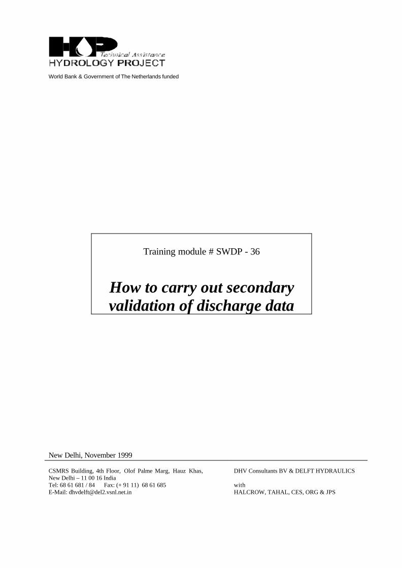
World Bank & Government of The Netherlands funded

Training module # SWDP - 36

How to carry out secondaryvalidation of discharge data

New Delhi, November 1999

CSMRS Building, 4th Floor, Olof Palme Marg, Hauz Khas,New Delhi – 11 00 16 IndiaTel: 68 61 681 / 84 Fax: (+ 91 11) 68 61 685E-Mail: [email protected]

DHV Consultants BV & DELFT HYDRAULICS

withHALCROW, TAHAL, CES, ORG & JPS

HP Training Module File: “ 36 How to carry out secondary validation of discharge data.doc ” Version 15/02/02 Page 1

Table of contents

Page

1. Module context 2

2. Module profile 3

3. Session plan 4

4. Overhead/flipchart master 5

5. Handout 6

6. Additional handout 8

7. Main text 9


1. Module contextWhile designing a training course, the relationship between this module and the others,would be maintained by keeping them close together in the syllabus and place them in alogical sequence. The actual selection of the topics and the depth of training would, ofcourse, depend on the training needs of the participants, i.e. their knowledge level and skillsperformance upon the start of the course.


2. Module profile

Title : How to carry out secondary validation of discharge data

Target group : Assistant Hydrologists, Hydrologists, Data Processing CentreManagers

Duration : One session of 60 minutes

Objectives : After the training the participants will be able to:Carry out secondary validation of discharge data

Key concepts : • Scrutiny of data in tabular and graphical form• Validation against data limits• Scrutiny of observed water level and computed discharges• Scrutiny of multiple graphs from adjacent stations• Graphical plot of balances• Graphical comparison of areal rainfall and discharge

Training methods : Lecture, software

Training toolsrequired

: Board, OHS, Computer

Handouts : As provided in this module

Further readingand references

:


3. Session plan

No Activities Time Tools1 General

• Overhead - highlighted text (2)5 min

22.1

Single station validationValidation against data limits• Overhead - Highlighted text• Overhead - Fig. 1 Table of values outside specified

boundaries

10 min

2.2 Graphical validation• Overhead - Highlighted text - points 1 to 4• Overhead - Fig. 2 Hydrograph of stage and discharge• Overhead - Highlighted text point 5 and bullets• Overhead - Fig. 3 Time series plots showing abrupt

discontinuities• Overhead - Fig. 4 Time series plots showing suspect

values

2.3 Validation of regulated rivers• Overhead - Highlighted text

min

33.1

Multiple station validationComparison plots• Overhead - Highlighted text

10 min

3.2 Residual series• Overhead - Highlighted text and equation• Overhead - Fig. 5 - Comparison plot of two stations and the

residual

3.3 Double mass curves• Overhead - highlighted text

4. Comparison of streamflow and rainfall


4. Overhead/flipchart master


5. Handout


Add copy of Main text in chapter 8, for all participants.


6. Additional handoutThese handouts are distributed during delivery and contain test questions, answers toquestions, special worksheets, optional information, and other matters you would not like tobe seen in the regular handouts.

It is a good practice to pre-punch these additional handouts, so the participants can easilyinsert them in the main handout folder.


7. Main text

Contents

1. General 1

2. Single station validation 1

3. Multiple station validation. 4

4. Comparison of streamflow and rainfall 6


How to carry out secondary validation of discharge data

1. General• Secondary validation of discharge will be carried out at Divisional offices on

completion of transformation of stage to discharge at the same office. Thedischarge series will contain flagged values whose accuracy is suspect (based onassessment of stage), corrected, or missing. These will require to be reviewed,corrected, or inserted.

• The quality and reliability of a discharge series depends primarily on the quality ofthe stage measurements and the stage discharge relationship from which it hasbeen derived. In spite of their validation, errors may still occur which show up indischarge validation. Validation flags which have been inserted in the validation of thestage record are transferred through to the discharge time series. These include the dataquality flags of ‘good’, ‘doubtful’ and ‘poor’ and the origin flags of ‘original’, ‘corrected’and ‘completed’. This transfer of flags is necessary so that stage values recognised asdoubtful or poor can be corrected as discharge.

• Discharge errors may also arise from the use of the wrong stage dischargerelationship, causing discontinuities in the discharge series, or in the use of thewrong stage series.

• Validation of discharge is designed to identify such problems. The principalemphasis is in the comparison of the time series with neighbouring stations butpreliminary validation of a single series is also carried out against data limits andexpected hydrological behaviour.

• Validation using regression analysis and hydrological modelling is specificallyexcluded from this module. They are considered separately in later modules.

2. Single station validationSingle station validation will be carried out by the inspection of the data in tabular andgraphical form. The displays will illustrate the status of the data with respect to quality andorigin, which may have been inserted at the stage validation stage or identified at dischargevalidation. Validation provides a means of identifying errors and, following investigation, forcorrecting and completing the series.

2.1 Validation against data limits

Data will be checked numerically against, absolute boundaries, relative boundaries andacceptable rates of change, and individual values in the time series will be flagged forinspection.

• Absolute boundaries: Values may be flagged which exceed a maximum specified by the user or fallbelow a specified minimum. The specified values may be the absolute values of thehistoric series. The object is to screen out spurious extremes, but care must be taken notto remove or correct true extreme values as these may be the most important values inthe series.


• Relative boundaries:A larger number of values may be flagged by specifying boundaries in relation todepartures (αα and ββ) from the mean of the series (Qmean) by some multiple of thestandard deviation (sx), i.e.

Upper boundary Qu = Qmean + α sx

Lower boundary Ql = Qmean - β sx

Whilst Qmean and sx are computed by the program, the multipliers α and β are inserted bythe user with values appropriate to the river basin being validated. The object is to setlimits which will screen a manageable number of outliers for inspection whilst givingreasonable confidence that all suspect values are flagged. This test is normally onlyused with respect to aggregated data of a month or greater.

• Rates of change.Values will be flagged where the difference between successive observationsexceeds a value specified by the user. The specified value will be greater for largebasins in arid zones than for small basins in humid zones. Acceptable rates of rise andfall may be specified separately, generally allowable rates of rise will be greater thanallowable rates of fall.

For looking at the possible inconsistencies, it is very convenient if a listing of only those datapoints which are beyond certain boundaries is obtained. An example is given in Table 2.1

Table 2.1 Example of listing of data exceeding given limits

Series KHED_QH less than 0 or greater than 1,500 Month 8

==========Data========== Year month day hour sub.i Value

1997 8 23 9 1 1918. + 1997 8 23 10 1 1865. + 1997 8 23 11 1 1658. +

2.2 Graphical validation

• Graphical inspection of the plot of a time series provides a very rapid and effectivetechnique for detecting anomalies. Such graphical inspection will be the mostwidely applied validation procedure and will be carried out for all discharge datasets.

• The discharge may be displayed alone or with the associated stage measurement(Fig. 2.1). Note that in this example the plot covers 2 months to reveal any discontinuitieswhich may appear between successive monthly updates updates of the data series.

• The discharge plots may be displayed in the observed units or the values may belog-transformed where the data cover several orders of magnitude. this enables valuesnear the maximum and minimum to be displayed with the same level of precision. Log-transformation is also a useful means of identifying anomalies in dry season recessions.Whereas the exponential decay of flow based on releases from natural storage arecurved in natural units, they show as straight lines in log-transformed data.


Figure 2.1 Q(t) and h(t) of station Khed for consecutive months

• The graphical displays will also show the absolute and relative limits. The plotsprovide a better guide than tabulations to the likely reliability of such observations.

• The main purpose of graphical inspection is to identify any abrupt discontinuitiesin the data or the existence of positive or negative ‘spikes’ which do not conformwith expected hydrological behaviour. It is very convenient to apply this testgraphically wherein the rate of change of flow together with the flow values are plottedagainst the expected limits of rate of rise and fall in the flows. Examples are:

v Use of the wrong stage discharge relationship (Fig. 2.2). Note that in this example,discharge has been plotted at a logarithmic scale

v Use of incorrect units (Fig. 2.3)v Abrupt discontinuity in a recession (Fig. 2.4).v Isolated highs and lows of unknown source (Fig. 2.5) but may be due to recorder

malfunction with respect to stage readings

Figure 2.2 Use of incorrect rating for Figure 2.3 Use of incorrect units part of the year


Figure 2.4 Unrealistic recession Figure 2.5 Isolated ‘highs’ and ‘lows’

2.3 Validation of regulated rivers

The problems of validating regulated rivers has already been mentioned with respectto stage data and should also be borne in mind in validating discharge data. Naturalrivers are not common in India; they are influenced artificially to a greater or lesserextent. The natural pattern is disrupted by reservoir releases which may have abruptonset and termination, combined with multiple abstractions and return flows. Theinfluences are most clearly seen in low to medium flows where in some rivers thehydrograph appears entirely artificial; high flows may still observe a natural pattern. Officersperforming validation should be aware of the principal artificial influences within the basin,the location of those influences, their magnitude, their frequency and seasonal timing, toprovide a better basis for identifying values or sequences of values which are suspect.

3. Multiple station validation.3.1 Comparison plots

The simplest and often the most helpful means of identifying anomalies betweenstations is in the plotting of comparative time series. HYMOS permits the plotting ofmultiple for a given period in one graph. There will of course be differences in the plotsdepending on the contributing catchment area, differing rainfall over the basins and differingresponse to rainfall. However, gross differences between plots can be identified.

The most helpful comparisons are between sequential stations on the same river. Theseries may be shifted relative to each other with respect to time to take into account thedifferent lag times from rainfall to runoff or the wave travel time in a channel.

In examining current data, the plot should include the time series of at least theprevious month to ensure that there are no discontinuities between one batch of datareceived from the station and the next - a possible indication that the wrong data have beenallocated to the station.

Comparison of series may permit the acceptance of values flagged as suspectbecause they fell outside the warning ranges, when viewed as stage or when validated as asingle station. When two or more stations display the same behaviour there is strongevidence to suggest that the values are correct, e.g. an extreme flood peak.


Figure 3.1 Plot of multiple discharge series of adjacent stations

Comparison plots provide a simple means of identifying anomalies but notnecessarily of correcting them. This may best be done through regression analysis,double mass analysis or hydrological modelling.

3.2 Residual series

An alternative way of displaying comparative time series is to plot their differences.This procedure may be applied to river flows along a channel to detect anomalies inthe water balance. HYMOS provides a means of displaying residual series under the option‘Balance’. Both the original time series and their residuals can be plotted in the same figure.

Water balances are made of discharge series of successive stations along a river or ofstations around a junction, where there should be a surplus, balance or deficit depending onwhether water is added or lost. The basic equation is expressed as:

Yi = ±a.X1,i ± b.X2,i ± c.X3,i ± d.S4,i

where:a, b, c, d = multipliers entered by the user (default = 1)± = sign entered by user (default = +)

A maximum of four series is permitted. An example for the series presented in Figure 3.1 isshown in Figure 3.2 where the comparison is simply between two stations, upstream and adownstream. Reference is also made to module 30. Any anomalous behaviour should befurther investigated. Sharp negative peaks may be eliminated from the plot by applying theappropriate time shift between the stations or to carry out the analysis at a higheraggregation level.


Figure 3.2 Example of water balance between two adjacent stations

3.3 Double mass curves

Double mass curve analysis has already been described in the secondary validationof rainfall (Module 9) and climate (Module 17). It can also be used to show trends orinhomogeneities between flow records at neighbouring stations and is normally usedwith aggregated series.

A difficulty in double mass curves with streamflow is in the identification of which ifany station is at fault; this may require intercomparisons of several neighbouring stations.There may also be a legitimate physical reason for the inhomogeneity, for example, theconstruction of a major irrigation abstraction above one of them. In the latter case nocorrection should be applied unless one is attempting to ‘naturalise’ the flow. (Naturalisationis the process of estimating the flow that would have occurred if one, several or allabstractions, releases or land use changes had not occurred).

4. Comparison of streamflow and rainfallThe principal comparison of streamflow and rainfall is done through hydrologicalmodelling. However, a quick insight into the consistency of the data can be made bygraphical and tabular comparison of areal rainfall and runoff. The computation of arealrainfall is described in Module 11; it will be realised that areal rainfall is also subject to errorwhich depends upon the density of stations within the basin and the spatial variability ofrainfall. Basically the basin rainfall over an extended period such as a month or year shouldexceed the runoff (in mm) over the same period by the amount of evaporation and changesin storage in soil and groundwater. Tabular comparisons should be consistent with suchphysical changes. For example an excess of runoff over rainfall either on an annual basis orfor monthly periods during the monsoon will be considered suspect.


Graphical comparison on a shorter time scale can be made by plotting rainfall andstreamflow on the same axis. In general the occurrence of rainfall and its timing should befollowed by the occurrence of runoff separated by a time lag but precise correspondenceshould not be expected owing to the imperfect assessment of areal rainfall and to thevariable proportion of rainfall that enters storage.

Download-manuals-surface water-waterlevel-36howtocarryoutsecondaryvalidationofdischargedata

Technology

Transcript of Download-manuals-surface water-waterlevel-36howtocarryoutsecondaryvalidationofdischargedata