Double-Porosity Modelling of Groundwater Flow

Through Fractured Rock Masses

by

Doina Maria Priscu

Department of Mining and Metallurgicai Engineering

McGill University, Montreal, July 1997

A thesis submitted to the Faculty of Graduate Studies and Research in

partid fulfillment of the requirements of the degree of Master of Engineering

O Doina Maria Priscu, 1997

National Library 1*1 of Canada Bibliothèque nationale du Canada

Acquisitions and Acquisitions et Bibliographic Services services bibliographiques

395 Wellington Street 395. rue Wellington Ottawa ON K1A ON4 Ottawa ON K1 A ON4 Canada Canada

Your fi& Votre rtifersnce

Our Ne Notre refdrence

The author has granted a non- L'auteur a accordé une licence non exclusive licence allowing the exclusive permettant à la National Library of Canada to Bibliothèque nationale du Canada de reproduce, loan, distribute or sell reproduire, prêter, distribuer ou copies of this thesis in microfoq vendre des copies de cette thèse sous paper or electronic formats. la fome de microfiche/Wn, de

reproduction sur papier ou sur format électronique.

The author retains ownership of the L'auteur conserve la propriété du copyright in th is thesis. Neither the droit d'auteur qui protège cette thèse. thesis nor substantial extracts fkom it Ni la thèse ni des extraits substantiels may be printed or otherwise de celle-ci ne doivent être imprimes reproduced without the author's ou autrement reproduits sans son permission. autorisation.

ABSTRACT

One of the key factors in ensuring safe slopes in open pit mines is the control of the groundwater flow

w i t b the slope. When analyzing the flow regime and its chatacteristics, traditional numerical

methods designed for soil-Iike rnaterials may not aiways apply. In the present thesis, the two-

dimensional finite element code FbwD was developed to analyze steady-state seepage through

hctured rock masses, under saturated conditions. The program provides the user with two

m o d e b g options: porous (soil) rnaterials, or fiactured rock masses. The double-porosity model was

incorporated in the code, in order to better model flow through anisotropic, heterogeneous fktctured

rock masses, where Dirichlet and Neumann boundary conditions can apply. FlowD program

calculates total pressure head, flow gradients and velocities within the specified domain. Drains,

drainage galleries and wells, as well as aquifer recharge can be simulated. A real large-scde case

study, with complex geologicd features has been simulated in order to demonstrate the application of

the double porosity model. Three different scenarios have k e n modeled for the same slope , which

are natual groundwater regime, vertical well simulation, and drainage galleries simulation. The results

show good agreement with the predictions of both the consultant and the mine's engineering division.

La percolation de l'eau souteraine dans les talus rocheux des mines à ciel ouvert est l'un des

facteurs les plus importants à considérer vis-à-vis de la stabilité des pentes. Dans les analyses du

régime d'écoulement des eaux souterraines et de ses caractéristiques dans les talus rocheux, les

méthodes numériques traditionnelles, conçues pour des matériaux granulaires, ne sont pas

toujours applicables. Dans cette thèse, un programme à éléments f i s à deux dimensions,

RowD, a été conçu afin de permettre l'analyse de l'écoulement à travers les milieux rocheux

fracturés ou les milieux granulaires poreux. Un modèle à double porosité a été incorporé dans le

code-source, afin de permettre une meilleure modélisation de l'écoulement à travers un milieu

rocheux fracturé, anisotrope et hétérogène, où les conditions des frontière de type Dirichlet et

Neumann sont applicables. Le logiciel FlowD calcule les pressions totales, les gradients et les

vitesses de l'écoulement de la région étudiée. Les forages, les galeries de drainage, ainsi que les

recharges de l'aquifère peuvent aussi être modélisées. Une étude d'un cas réel à grande échelle,

ayant une géologie complexe, a été effectuée pour valider et démontrer I'appiicabilité du modèle

à double porosité. Trois différents scénarios ont été ainsi simulés: le régime nanirel, l'existence

d'un puits, puis celle de deux galeries de drainage dans le même talus rocheux. Les résultats

obtenus concordent avec les prévisions du consultant et du département d'ingénierie de la

companie minière.

The author wishes to give her warm thanks, and to acknowledge support of the folIowing persons,

without whom this thesis would not be completed:

Professor Hani Mitri, rny s u p e ~ s o r , for his guidance and patience thmughout my entire MEng.

Program, and for dowing me to use the FELIBS library, and e-z tuoh mesh generator and pre-

processor. Besides the technical advice, his friendship made a great difference in my work.

Mr. Yves Beauchamp, SIope stability engineer, LAB Chrysotile, Black Lake Mine, Québec, for his

assistance and time. Data supplied from the mine was crucial in my thesis, for progran validation.

Professor René Thenien , Lavai University, Quekc, for his advice in the application of the double-

porosity model.

My colleagues from the Numencal Modeiing Laboratory, for making my life easier during the long

days spent at McGU.

The management personnel and my colleagues in CANMET, for allowing me to use part of the

equipment and graphical software, as well as for their constructive ideas.

Caius Priscu, my good coileague and beloved husband, for his understanding, support, for ail the

evenings and weekends that we spent together in &nt of a cornputer, when many other thùigs

could have been done.

TABLE OF CONTENTS

ABSTRACT

RESUME

ACKNOWLEDGEMENTS

LIST OF FIGURES

LIST OF TABLES

1 . INTRODUCTION ....................................................................................... 1.1

1.1 General ..................................... ,.. ............................................................................... 1.1

1.2 Objectives and methodology ................................................................................. 1.2

2 . BASIC CONCEPTS OF GROUNDWATER FLOW ............................................................. 2.1

2.1 Generai groundwater classification ............................................................................ 2.1

2.2 Overview of flow phenornena .................................................................................... 2.4

2.3 Groundwater 8 ow equation in porous media ........................................................... 2.14

3 . ROCK MASS AND DISCON'IINWTY MODELS IN HYDROGEOLOGY ........................ 3.1

3.1 Introduction ................................................................................................................ 3.1

3.2 Rock mass characterization ........................................................................................ 3.1

3.3 Characterization of discontinuities ............................................................................. 3.6

3.4 Models in hydrogeology ........................................................ 3.11

4- DOUBLE-POROSIT'Y MODEL FOR FLOW IN FRACTURED ROCKS ............................ 4.1

......................................................................................................... 4.1 Introduction .....4.1

............................................................................................ 4.2 HydrauIic conductivity 4.1

4.3 Flow velocity ............................................................................................................. 4.4

4.4 Flow in fkactured media ........................................................................................... 4.6

4.5 The double-porosity mode1 ......................................................................-............... 4.10

5 . FlowD FIME ELEMENT CODE ................ ... .................................................................. 5.1

5.1 Flow equations . anaIytical formulations ................................................................... 5.1

5.2 The quadrilateral isoparametric element ................................................................... 5.5

5.3 Finite element formulation ......................................................................................... 5.8

......................................................................................................... 5.4 Equation soiver 5.12

.............................................................................................. 5.5 FIowD cornputer code 5.13

.................................................................... 6 . MODEL VERIFICATION ANF APPICATION 6 .1

............................................................................................. 6.1. FlowD code verification 6.1

.................................................................................................................. 6.2 Case study 6 .2

6.2.1 East waii of BIack Lake Mine ................................................................ 6.3

6.2.2 Slope geometry and hydrogeologicd regime ......................................... 6.6

7 . CONCLUSIONS AND RECOMMANDATIONS FOR FURTHER RESEARCH ................ 7.1

8 . REFERENCES ........................................................................................................................ 8.1

APPENDIX A . User's Manual

APPENDM B . FlowD computer code listing

List of figures

Figure 2.1 General groundwater classification

Figure 2.2 Physicd properties as might be measured for increasing sample volume

(Themen, 1994)

Figure 2.3 Range of validity of Darcy's Law (Therrien,1994)

Figure 2.4 Schematic representation of fractwed medium (Bear et al., 1993)

Figure 3.1 Classification of discontinuities using descriptive - structural criteria (Thiel,1989)

Figure 3.2 Types of media occurring in rock masses (Louis, 1976)

Figure 3.3 Models in hydrogeology

Figure 4.1 D e f ~ t i o n of representative elementary volumes for the fractures and porous block

domain (Bear and Berkowitz, 1987)

Figure 4.2 Coexistence of two pûrosities as random double porosity (Sen, 1995)

Figure 4.3 A fractured medium. The low-permeable porous mat& is dissected by a system of

high-conductive fractures which have a small storage capacity (Barenblatt, 1990)

Figure 5.1 Hydraulic conductivity direction for soi1 material

Figure 5.2 Global system of coordinates for hydraulic conductivity tensor (de Marsily, 1986)

Figure 5.3 Isoparametric 4-node element in the global and local systern of coordinates

Figure 5.4 Hydraulic conductivity of sets of fractures

Figure 5.5 Distnbuted flux over the side of an element

Figure 5.5 Numencal integration scheme

Figure 5.6 Flowchart of the computer code FlowD

Figure 5.7 Types of analysis performed by FlowD

Figure 6.1 B Pit Mine location (Mine reports)

Figure 6.2 B Pit Mine geological plan view (Mine reports)

Figure 6.3 Schematic flow diagram ( m e reports)

Figure 6.4 Generated mesh for the FE andysis

Figure 6.5 Materials identified in the 5000N Section

Figure 6.6 Groundwater flow velocity

Figure 6.7 Total head - 5000N Section - Regional groundwater regime

Figure 6.8 Total head - 5000N Section - Weli simulation

Figure 6.9 Total head - 5000N Section - Drainage galiery simulation

List of tables

Table 3.1 Rock mass classification with respect to basic characteristics (Goodman, 1976)

Table 3.2 Rock mass classification with respect to dry density and porosity (ISRM, 1978)

Table 3.3 Rock mass classification according to joint spacing and RQD (Theil, 1989)

Table 3.4 Estimation of secondary permeability fiom discontinuity fiequency (Goodman, 1976)

Table 3.5 Permeability iimits (Goodman, 1976)

Introduction

Surface mining is one of the oldest forms of rnining around the world. In the early days of mineral

extraction, it was the easiest, safest and most affordable mining method being widely used in srnail

scale mining operations. In recent years, surface mining has attained great depths, which implies

new problems related to this activity.

Costs of ore recovery have increased considerably, but new technology was developed in order to

help the rnining industry. New sciences have been developed in order to help and better understand

different aspects related to this form of mining. Geological formations have a better descnption and

the geophysical concepts can give interpretations of discontinuities' pattern. New rock mechanics

concepts have been established, that help explain rock mass behavior. Hydrogeology as an

engineering science, in particular, has taken new steps in explaining water influence on the eaah

crust behavior.

Open pit operations have become, in the last few years, chalienging engineering projects, mainly

due to the large pit sizes and ore recovery methods. These issues have Ied to the development of a

variety of engineering tools that have become necessary to meet the needs of the mining industry.

Hydrogeology and rock rnechanics sciences attempt to better understand phenornena that occur in

rock masses. The water interaction with different types of geological fomations changes the

behavior of rock itself. Rock mass characterization and discontinuities' descnption is needed to

apply safe and economic mùiing methods. Particularly, e n g i n e e ~ g design of high slopes in open

pit mines bas to take into consideration ail of the above mentioned factors.

In pit slope stabîiity problems, monitoring of hydrogeological regime plays a major role in

evaluating safety. In most cases, groundwater regime should be welI understood in combination

with rock mechanics characterization of geological formations. These aspects have to be addressed

in order to solve en,@eering problems related to water table, water pressure, water innows and

poor drainage, and structural anomalies in rock dope that cm affect their stability. In general,

continuous monitoring and depressurization reduce failure risks. These tasks are not always easy to

achieve, and in some cases they become mandatory for efficient and safe mining operations.

Seepage Iaws in fiactured media were formdated fiom the original groundwater laws in soil

materials. They were completely reviewed to take into account the flow phenomenon in fractured

media. Rock mass and discontinuity characterization were needed in order to look into

hydrogeological models. Various rnodels have been proposed for both rock mass and flow

phenomenon. These models are briefly reviewed with respect to their applicability to surface

mining related problems.

1.2 Ob-iectives and methodologv

The objective of this research is to develop an easy tool, in the fom of a computer code, that WU

simulate confined groundwater flow in fractured rock slopes. Different assumptions had to be made

related to the rock itself, structural discontinuities, and the flow regime.

The use of numerical modeling in combination with slope monitoring systems can give good

feedback in designing and operating large open pit slopes. In this idea, a simple tool to estimate

groundwater flow through a f'ractured rock mass is proposed in this thesis, that c m be easily used in

a mining operation environment. Fractured rock slopes geornew, discontinuities' pattern and

charactenstics, as weil as rock mass behavior were the main aspects to include with the tool.

FlowD code is a f ~ t e element computer program for two-dimensional seepage analysis. It

employs 4-node isoparametric elements, uses 4x4 integration scheme. It performs seepage analysis

in soi1 or rock slopes. Double-porosity mode1 was used to simulate flow in the rock media.

Discontinuities' orientation (dip/dip direction), aperture, average number of fractures and their

permeability descnbe their pattern in the slope. The rock blocks were considered with very low

permeability that c m be nii compared to the discontinuities' permeability.

Verifications of this code were made on literature examples. An open pit slope was modeled with

the data from Black Lake Mine, LAB Chrysotile Inc., Québec.

Basic concepts of groundwater flow

2.1 General groundwater classification

Water is often present in geologic media of the earth crust. Groundwater may be defmed as the

whole amount of water which is stationary or flows through the ground surface of the earth. In

addition to its physico-chernicd effects, its influence on the mechanical behavior of the soi1 or

rock masses is of utmost importance. The presence of water flowing in the underground implies

the existence of water pressure and seepage forces which have to be taken into consideration

when various geotechnical problems are considered.

Subsurface waters are classified in different ways, considering their various properties as the

classification basis, i.e. temperature, chemicai composition, movement character, origin, etc. A

generd classification of groundwater is ilfustrated in Figure 2.1 flowchart and is based on the

origin of groundwater, the occurrence depth and different types of rock formations. This

classification shows only water which is stationary in the ground, but at the same time, water c m

move through the porous media and rock formations. From an engineering point of view, both

forms of water in the ground are important because there is an interaction between water and

media, with repercussions on the media's properties. This study will consider only the

groundwater that moves freely in the underground.

When studying the groundwater movement, the place of movement, the time dependency and

the type of flow must be taken into consideration. The water flow problem is actuaily divided

into two groups: saturated flow when different media are completely saturated with water

meaning dl pores are filled with water, and unsaturated flow when voids are partially fded with

water and partially with air. A third group is actualiy a combination of these two, when flow is

saturated in part of the domain and unsaturated in another.

G R O U N D W A T E R O C C U R R E N C E

grave1 sand silt clay

above water table

below water table

1 limesione 1 1 dolomite 1

~'JFIFI water water of rocks water water

Figure 2.1 General groundwater classification

al1 other formations I water water

1

shallow deep position position

Other weil-known classification methods used for groiindwater flow are different types of

problems like: dimensional character of flow, time dependency of flow phenornena, boundaries

of flow domain, or medium and fluid properties.

The flow regime can be detennined by using the Reynold's number (Re) which will be discussed

later in this chapter. It can be steady or unsteady depending on t h e factor: steady when the flow

parameters remain constant d u ~ g a period of time and unsteady when the flow parameters

change with time. Flow can be laminar, non-laminar, or turbulent. Fluid charactenstics are

important in solving fiow equations and its properties should, if possible, be determined a prion

in any further study .

The flow of groundwater is produced by different forces; the most important are gravity and

pressure forces. Meanwhile, some other forces can produce water movement like therrno-

osmoses forces, being the result of differences in temperature in the unsaturated zone. The

increase of surface tension which accompanies the decrease in temperature can cause water

movement. At the same time, the increase in surface tension causes a greater capillary attraction

in the heat flow direction. The actud flow of water under temperature gradient is probably a

combination of c a p i l l q and vapor transport. If two types of water have different dissolved

solids concentrations, and if they are separately by a semipermeable membrane, water will rnove

from the low concentration side to the high concentration side. The movement will continue u n d

concentrations are the sarne or until some other counteracting forces, such as hydrostatic

pressure, balance the chernical forces. The tendency of water to move in the direction of

increasing chemicai concentration is called osmosis.

In recent years, the new groundwater contamination studies have addressed other types of

problems, such as site remediation, with many appLications in waste disposal. As long as the

groundwater is conthminated with reactive or non-reactive contarninants, it can transfer the latter

to the medium through contaminated groundwater flows.

2.2 OveMew of flow phenornena

Linex flow Iaws - Darcy's Law

The basic relationship of the subterrain hydrodynamics, the seepage law, establishes the

relationship between the seepage velocity and the pressure field thar generates the flow. This

relationship was discovered experimentaiiy in 1856 by a French engineer, Henry Darcy, who

formulated it for one dimensional flow in an isotropie and homogenous porous medium,

where: Q = flux of water discharge through porous medium t3~']; A = area of the cross section closed in the porous medium b2];

Ah = difference in hydraulic head between the measurements points [LI;

L = distance between the measurernents points CL];

K = hydrauiic conductivity or coefficient of perneability which depends on the Buid

properties and porous medium @X1];

i = hydraulic gradient &/LI.

Darcy's Law was Iater derived fiom the Navier-Stokes equations by rneans of their statistical

integration (Slattery, 1972, and Greenkorn, 1982). This study does not contain details about the

demonstrations of Darcy's Law but, it wiIl cover its different formulations and limitations.

Fluid flow in a porous medium differs from the fluid motion considered in ordinary

hydrodynamics, because, in any open macro volume, there is immovable solid phase ( the solid

ma&, or skeleton) at the boundary of which the fluid is dso immovable. In the latest

demonstration of Darcy's Law, the porous medium is regarded as a system of pore channels of an

elementary macro volume which is hydrodynamicaüy equivalent to a system of interconnected

tubes. Flow velocity characterizes discharge through this system. On the other hand, the

discharge is determined by pressures at the channel entries and exits. Since the bulk discharge is

the sum over many channels, it is govemed by the pressure &op, Le. by the gradient of the fiuid

mean pressure.

When considering the small velocity of an arbitrary point of the porous medium, the flow

velocities field c m be assumed to be continuous and al1 porous medium and fluid parameters c m

be assumed to be constant. Only pressure variation that is very small, can not be nucleated,

because if the pressure does not exist or is constant over the space, the flow is absent. The basic

assumption leading to the seepage law statement is as follows: the pressure gradient at a given

point of porous medium is governed by the seepage flow velocity vector as well as by the fluid

and porous medium properties.

Before extending Darcy's Law to a three-dimensions analysis a few basic definitions regarding

porous media and flow phenomena must be given. Porous media can be characterized as

homogenous or heterogeneous, as welI as isotropic or anisotropic.

Homogenous: medium properties do not change from one place to another Le. they are

independent of location.

Heterogeneous: medium properties vary spatidy and are dependent on location.

Isotropie: medium properties are independent of the measurement direction.

Aaisotropic: medium properties Vary with measurement direction within the formation or

geologic units.

Here are the four possible combinations of anisotropy and heterogeneity:

Homogeneous - isotropic;

Homogeneous - anisotropic;

Heterogeneous - with different isotropic layers;

0 Heterogeneous - anisotropic.

The extension of one-dimensional Darcy's Law to three-dimensions law is:

v = - K ( V p - p g )

where: v = velocity tensor;

K = hydraulic conductivity tensor;

p = hydrostatic pressure m2]; p= density of the fluid m3]; g = gravitational acceleration ~ / T 2 ] .

In the formula above porous medium is homogenous and isotropic; flow takes place in a

saturated zone, and the Buid motion is inertialess. If the medium is anisotropic and inertia effects

are considered, the formulation of Darcy's Law will differ.

In most of Darcy's Law formulations hydraulic conductivity is a second rank tensor. Its

romponents depend on the characteristics of porous medium as well as on fluid properties.

Science domain and matenal properties deterrnine the formulation of this law. As an example in

1931, Richards formulated the expression of Darcy's Law for unsaturated zone used in

geotechnical engineering:

where: 0 = 0(y) moisnire content [dirnensionless];

K = K (8) or K= (y) unsaturated hydraulic conductivity &/Tl;

y = pressure head CL];

t = time [Tl;

z = elevation fkom the arbitrary datum E].

Variables are moisture content, pressure head and hydraulic conduc tivity. In recent years , there

has been considerable work involving flow in unsaturated media with applications, particularly in

waste disposal.

Darcy's Law holds well in most practical situations like:

1. saturated flow;

2. steady-state flow;

3. transient flow;

4. flow in heterogeneous and misotropic porous media;

5. flow in gmular media.

In some cases, the validity of this law is questionable. A plot of the groundwater velocity versus

hydraulic conductivity gradient would reveal a straight line for ali gradients between O and -, if

heari ty is maintained. For granula material flow, there are at least two situations where the

validity of this linear relationship is questionable: flow through low permeabiiity sediments

under very low gradients and high flow rates through highly permeable media.

The fxst major concem of Darcy's Law is the macroscopic behavior. This assumption refers to

the lower limit of this law. In a porous media considered, one has to be able to sample

meaningfuul values for physical properties that are averaged over a volume sample and the

Darcy's Law is valid. If not, the applicability of this law is under question. It is shown in

Figure 2.2 that this volume sarnple is referred to as a Representative Elemental Volume (or REV)

(Freeze et al., 1979). To apply Darcy's Law, three conditions has to be met:

1. One must be able to define REV which is homogenous;

2. One must be able to characterize the ensemble of grains as a continuum;

3. The continuum must be macroscopic.

1 I

4 Microscopic I ,, 1 I

- Macroscopic P

I t 1 1 1 1 I heterogenous

homogenous

1 1

0 .1 b

Volume

Figure 2.2 Physicai properties as it might be measured for increasing sample volume

(Themen, 1994)

The second major concern of Darcy's Law is the flow rate. If this law is universal, flow would

occur for a!l infinitesimal gradients in low permeable materials, and laminar flow would occur

for high flow rates under high gradients in permeable materials. Figure 2.3 illustrates Darcy's

Law and its validity range.

For low permeability fine-grained materials, it has been suggested, based on laboratory evidence,

that there may be a threshold hydraulic gradient below which there is no fiow. Swartzendmber

(1962) and Bolt et al. (1969) reviewed the evidence and sumrnarized the phenomena-

threshold gradient

n o n - l inear ( turbulent)

threshold gradient

Figure 2.3 Range of validity of Darcy's Law (Therrien,1994)

Of greater practicai importance is the upper M t on the range of validity of Darcy's Law. At very

high flow rates, the linear law breaks down. This evidence is reviewed in detail by Todd (1959)

and Bear (1972). The upper limit is identified with Reynold's number (Re), a dimensionless

nurnber that expresses the ratio of inertiai to viscous forces during flow; it is defined for the flow

through porous media as:

where: p = density of the fluid m3]; v = specific discharge or velocity @ X I ;

p = dynamic viscosity of the fluid [MLT];

d = the representative length of a sarnple of porous medium CL].

This number is widely used in fluid mechanics to distinguish between laminar flow at low

velocities and turbulent flow at high velocities. In 1972, Bear sumrnarized the experimental

evidence with the foilowing statement: " Darcy's Law is valid as long as Reynold's number

based on average grain diameter is within the 1 to 10 range". For this range of Reynold's nurnber

flow through porous media is laminar and obeys the linear law.

Darcy's Law does not cover al1 solutions for groundwater flow. Deviations frorn the linear law

are due to either aquifer material composition or flow velocities leading to turbulent flow regime.

This situation c m be explained by the variation of hydraulic gradients, which increase

proportionaily with the specific discharge in a nonlinear manner. It is also the case when

velocities are increased, even in porous media. In coarse grained porous media and fractured

media due to relatively high hydraulic conductivity, groundwater flow may be turbulent.

Nonlinear flow laws

In fiacîured media, a nonlinear relationship was observed by h u i s (1969), Snow (1968) and

Maini (1971). The nonluiearity was attributed to different factors such as kinetic energy,

nonlinear pressure flow laws, leakage packers, and increase in fracture aperture. Both laws can be

surnrnarized as foilows:

where: v = seepage velocity v] ;

K = hydraulic conductivity &/Tl;

dWdl = hydrauiic gradient [L/L];

m= power of the hydraulic gradient;

m = 1 flow is iinear and laminar, (Darcy's Law);

m # 1 flow is nonlinear and turbulent (Louis, 1974).

Flow rates exceeding the upper Iimit of Darcy's Law are common in rock formations such as

karstic iimestone7s, dolomites and cavernous volcmic. Darcian fiow rates are almost nevcr

exceeded in nonindurated rocks and granular materials. Fractured rocks which are more

permeable through joints, fissures and cracks will be discussed later.

Other more or less empiricai nonlinear expressions have been proposed; generally expressed as:

where: v = specific discharge [Lm];

i = hydraulic gradient &IL];

a = parameter dependent on medium and fluid properties [TL]; 2 2 b = parameter dependent on medium and fluid properties [T /L 1.

Fractured medium fiow is quite different from the porous medium flow. Flow in an individual

fracture is rather similar to pipe flow. Different from porous media, the moving water particle is

not subjected to resistance everywhere, fractures' intersection are the major point were resistance

forces are developed. In highly fractured media fiow can be considered similar to that of porous

media, if the rock-fractures properties can be viewed as a common unit.

Flow laws in individual fractures were investigated by Louis (1974) for lamina and turbulent

flow by assuming a uniform flow velocity over the total aperture of the fracture. In any single

fracture, flow may be considered one-dimensional or two-dimensional. For the one-dimensional

flow, it c m be assumed to be paralle1 or nonparailel. When Stream lines are not parallel a two-

dimensional flow appears in the fracture.

The roughness of the fracture w d s plays a dominant role in a single fracture flow. This

parameter influences the flow re-@me and the validity of the Reynold's number. Louis (1974)

summarized flow laws in a single fracture in five different combinations of flow regimes and

roughness of the fracture, as rnentioned below:

1. Smooth-laminar flow regime (a linear low sirnilar to Darcy's Law);

2. Rough-lamuiar flow regime (the relative roughness plays an important role);

3. S mooth-turbulent flow regime (fracture aperture plays on important role) ;

4. Rough-turbulent flow regime (nonlineu flow law);

5. Very rough-turbulent flow regime (similar to the rough-turbulent fIow regime).

AU above mentioned flow laws follow the general law (2.5) with the flow gradient at a certain

power which is always less than one. AU these laws and their empirical formulations were

obtained under steady-state flow conditions similar to Darcy ' s Law.

In rock masses, the rock blocks are separated by fractures which may or may not be

interconnected (Figure 2.4). These fnctures have different directions and different apertures

(with no superiority one over other), and the rock mass is made of blocks of irregular size and

shape. Based on this idea, Barenbaftt et al. (1960) assumed in fomulating a new approach

growndwater flow, that any srnall volume of rock consists of a large number of porous blocks

as weIl as fissures.

Figure 2.4 Schematic representation of fiactured medium (Bear et d.,1993)

Therefore, within a small area of the same rock mas , there are two different media: fractures

and blocks. Their hydraulic behaviors are different, depending on the type of flow considered.

Under steady-state conditions, fiactures and blocks act together as one unit. In unsteady flow,

because fractures' hydrauiic conductivity is greater than blocks' hydrauiic conductivity and

kachues' storativity less than blocks' storativity, the whole rock mass must be considered as

consisting of two different but coexisting porous media with different hydraulic heads. Under

such conditions, three different types of flow will appear. These are: flow in the fractures, flow

in porous blocks, and flow fkom blocks to fractures. The flow law in the two mentioned media

can be linear or nonlinex, as described above. However, the same laws cannot be used for

block-to-fracture flow.

For the block-to-fracture flow, the law was formulated by Barenblatt et ai. (1960). In

forrnulating this law, they assumed that the flow is pseudo-steady state, and water exchange

between blocks and fractures depends only on the difference between the head in the fiactures,

hf, and the average head in the block, hb . No consideration is given to the blocks geometry.

This law is fonnulated as follows:

where: q = specific discharge [ LJT'];

ût= parameter depending on the geometry of the fractured rock [l/T];

hf = head in the fracture CL];

hb = head in the porous block CL].

Other laws for block-to-fracture are based on the geometry of the porous blocks. Different

restrictions could be imposed for block shapes, which can either be cubes or paraiielepipeds,

depending on the modd used.

Karstic media differ from the above mentioned cases, because the medium is very heterogeneous.

Water flows in a system of interconnected cracks, cavems, and channels. The flow could be

similar to flow in conduits (large pipes) but, in most cases, the water rnay not fill the whole cross

section, and the water may not be under pressure. In this medium, the presence of large cavities

and caves could suggest that the fiow can be either larninar or turbulent, and Darcy's Law in

g~anular medium is no longer valid. It is also possible that in time, the karstic features might c.

become larger and the fiow regime might change. Such cases should be each studied

individually.

2.3 Groundwater flow equations in porous media

The basic flow law in underground hydrology is Darcy's Law, which was analyzed in previous

sections (with its different forms). This law, combined with the law of conservation of mass,

results in the equation of continuity. The latter practicaily describes the conservation of mass

during the 80w through porous medium. The continuity equation for saturated groundwater flow

is as follows after introducing the Darcy's Law in the conservation of mass Iaw:

where: p = density of the water flowing m3]; g = gravitation acceleration [ L/T'];

q = porosity [%];

t = time [Tl.

In this section, some forms of the continuity equation are reviewed for granular materials under

different conditions. The steps foilowed in their derivation WU not be presented herein. The

solution of the relevant differential equations should take into account the boundary-value

conditions, and anaiytical or numerical methods should be used for solving the systern of

equations.

S teady State Saturated Flow

For steady state conditions, (flow is not time dependent and medium is saturated), groundwater

flow in a hornogenous and isotropie medium c m be described by the following equation :

where: h = h ( x, y, z) = hydraulic head [2],

x, y, z = coordinates of a point in a three-dimensional Cartesian system.

This equation is one of the fundamental partial differential equations known in mathematics-

Laplace's equation. Its solution in this case is a function h (x, y, z) that describes the hydraulic

head h at any point in a three dimensionai flow field and depends on boundary conditions

imposed.

Transient Saturated Flow

If the groundwater flow occurs in a heterogeneous anisotropic medium, the continuity equation is

expressed in a different way, in accordance with medium conditions, as follows:

where : h = h ( x, y, z ) = hydraulic head &];

x, y, z = coordinates of a point in the flow field;

S, = specific storativity of the porous medium [ dimensionless];

K = hydraulic conductivity ( tensor )-

The solution of this equation is a function h (x, y, z, t) which describes the hydraulic head at a

point in the field, at any time. If the medium is homogenous and isotropie this equation becomes:

and is known in mathematics as the difision equation. Any solution requires knowledge of the

hydrogeological parameters, K = hydraulic conductivity ml, n = porosity [%], cr = coefficient

of vertical compressibility and fluid properties [dimensionless], p = density of the fluid m3], p = dynamic viscosityFI/LT], and P, = isothermal volumetric compressibility of the fluid

When developing this equation, it is assumed that changes in stresses within geological media

occur ody vertically. These changes are included in the vertical compressibility parameter. Such

approach couples three-dimensional groundwater flow to one dimensional stress field. The more

general approach which couples three-dimensional groundwater flow system to a three-

dimensional stress field was exarnined in detail by Biot (L941).

Transient Unsaturated Flow

The partial differential equation which describes flow in a p h a l saturated medium must take

into account changes in moisture content. These changes will occur in time that will produce

complex changes in voids' space that are practicdy pores' expansion.

Like in the formulation of the Darcy's Law for unsaturated zone, the moisture content 0 is a

function of the pressure head y.f, and the hydraulic conductivity K = K (0) = K (v) is a function

of moisture content or pressure head. The equation has the foliowing fom:

where: C (v ) = specific moisture content [dimensionless];

= pressure head CL];

K = K(y) = hydraulic conductivity V I ; x, y, z = coordinates of a point in the flow field.

The solution of Equation (2.13) is the pressure head a function y = y (x, y, z, t). The equation is

known as Richard's equation and is only valid for the unsaturated zone when studying

groundwater flow. In a coupled saturated-unsaturated mode1 the Richard's equation should be

combined with the diffusion equation.

Rock mass and discontinuitv models in hydrogeology

3.1 Introduction

Discontinuities present in rock formations change the qualitative aspect of the rock mass and

affect its behavior. Dealùig separately with the discontinuities' characterization is the oniy way to

reach a point where the interaction between rock mass and discontuiuity can be analyzed.

Understanding the behavior of the rock-joints ensemble is extremely important when studying

80w in this type of medium.

This chapter presents the engineering properties of rock masses needed in groundwater flow

problems, foilowed by a description of discontinuities' characterization. An overview of flow

models used in hydrogeology to describe flow phenornena in rock masses, discontinuities, as

well as the interaction between the two is presented.

3.2 Rock mass characterization

A general rock mass characterization starts with a generai rock mass classification dividing rocks

into two major classes, intact (or continuous) rock and f?actured/jointed (or discontinuous) rock.

The properties used to classi@ rocks wiii vary according to the purpose of the study and may

include various criteria: shear strength, flexural strength, tende strength, elasticity, permanent

deferability, creep rate, water flow, water storage properties, in-situ stress, drillability, formations

characteristics, and sornetimes density, thermal expansion, mineralogy and color.

The aîms of a rock mass characterization, as described by Bieniawski (1986), are therefore:

identify the most significant parameters influencing the behavior of a rock mas ;

divide a particular rock mass formation into groups of similar behavior, i.e. rock mass

classes of various qualities;

provide a basis for understanding the characteristics of each rock mass class;

compare the experience of rock condition at one site to the conditions and experience

encountered at other sites;

denve quantitative data and guidelines for the engineering design;

provide a common ba i s between engineers and geologists.

Engineering characterization of rock masses may be examined from different viewpoints and

structured in different groups Like: general characterization and direct dassification. The füst

one is based on the geological structure of the rock mass and on its basic characteristics and

properties which are independent of the conditions that will occur to them later after

investigation. The second one is adjusted to the engineering problems in tunneling, mining, civil

engineering, etc.

General characterizations are usuaily made when building physical and mechanical models of

rock masses, whereas engineering properties are generaiiy defined after the constitutive models

have been chosen.

At the beginning of this century, when the study of rock masses was starting, scientists tried to

estabhsh procedures and guidelines in this new science. During the last decades, rock

engineering developed many tools to create a new image of rock and rock masses. Their effort is

now used in rock mass classification and characterization. Many classification systems have been

developed: "Rock Load" (Terzaghi,l946), RQD (Deere et a1.,1967), RMR (BieniawskiJ973,

modified 1979), etc.

When studying flow in fiactured rocks, the chancterization of the medium has a süong influence

over the description of flow phenornenon. Depending on the flow mode1 chosen, the

discontinuities' characterization and their oncoming parameters which affect seepage are very

important. Both play a major role in choosing a combine mode1 for further studies.

Engineering properties are presented with respect to flow phenornena in fractured rocks. The

geological aspect of the problem has an importance when establ ishg the physical and

mechanical behavior of the rock rnass. According to the International Society of Engineering

Geology, different guideIines are based on the following features which affect the physical and

mechanical properties of the rock:

1. the minera1 composition related directly to the weight of solids;

2. the structure and the texture, which determine the unit weight of the solids and

the rock porosity;

3. the water content and the degree of weathering, which describe the physical

condition of the rock and affect its strength, deformability and permeability.

In the categories above, it is assumed bat the physical and mechanical properties of a rock, in its

present state, result from different processes, such as: genesis, metarnorphism, tectonics and

surface weathering. Thanks to these processes, one can explain not only the lithological and

physical features of the rock, but also their locations on Earth. A proposed classification

distinguishes the following rock mass units according to the degree of homogeneity:

geotechnicd unit;

lithological unit;

Lithological cornplex.

In 1981, the International Society of Rock Mechanics (Bieniawski,l979) proposed that a basic

geotechnicd description of the rock masses should include the following characteristics:

1. rock name with a simplified geological description;

2. the layer thickness and fkacnires (discontinuities) that intercept the rock mas;

3. the unconfined compressive strength of the rock matenal and the angle of fiction of

the fkactures.

The classification proposed by the International Society of Rock Mechanics (ISRM, 1973 ) is

"less geological" in its character than the one presented above. It is based on compressive

strength, on the weathering degree and on joint spacing; the range values can be determined

relatively easily (compressive strength and joint spacing). As for the weathering degree, it can

only have a descriptive character and cannot assign any precise value. According to variations in

compressive strength, weathering degree and joint spacing, rock masses are divided into three

categories and five corresponding classes, which are Uustrated in Table 3.1 below.

Table 3.1 Rock m a s c l a ~ s ~ c a t i o n with respect ta basic characteristics (Goodman, 1976)

Compressive Class strength m a ] Class

Weaihering Joint degree Class spacing

[ml slight or no weathering

weathering dong joints Fz O. 1-0.3

w al1

total slight 0.3- 1 .O total moderate 1 F4 1 1.0-3.0

total heavy 1 F5 1 >3.0

Based on the three features above, and using an additional general geological classification, it is

relatively easy to estimate the quality of the rock mass. Many other classifications are available,

based on engineering cntena referring to specific works.

The velocity of seismic waves propagation throughout a rock mass is another critenon that can

be used to spLit rock masses in different classes. Its value is a function of the type of rock within

the rock mass and its mineral composition, density, elasticity, weathering degree and

compactness. According to this criterion, rock masses are divided into four groups: Limestones,

shiest and adesites, granites and gneiss, and finally sandstone.

Flow in fiactured rocks could take place either in the fracture or in the porous blocks. The

porosity of the solid rock depends on the size of the pore opening and is called "primary

porosity". The dry density and the pnmary porosity of the rock are the parameters controlling

flow phenornenon in the intact rock or through blocks. According to the International Society of

Engineering Geology in 1978, rocks have been classified in five classes as shown in Table 3.2.

Table 3.2 Rock classification according to dry density and porosity (ISRM, 1976)

l 2 1 1.8-2.2 1 10 w 1 30-15 1 high I 1 1 2.2-2.55 1 rnoderate 1 15-5 1 medium 1

Generdly, the rock structure is composed of pnmary and secondary pores. Some rock formations

have considerable primary porosity, which represents the expansion of pores formed between

4 .-

5

2.55-2.75 high

over 2.75 1 very high

5- 1 low

less than 1 very low

grains and microcracks. In fragmented rocks, porosity depends on whether the grain-size

distribution, shapes, mangement, cementation degree of the grains or water pressure. As for

sedimentary rocks, the prirnary porosity is relatively high and could significantly influence the

hydraulic behavior of the rock..

The rate of inactive primary pores is higher than the rate of fractures (secondary pores), but, in

most of the cases secondary pores control the flow through rock masses. The primary pores of

igneous and metamorphic rocks are generally negligible. Discontinuities found in rocks have the

greatest infîuence when defining the hydraulic properties of rock mass for m e r studies.

Hydraulic properties of rock masses will be discussed later in this chapter, af3er the

discontinuities characterization.

3.3 Characterization of discontinuities

The presence of discontinuities in rock formations distinguishes rock kom rock mus. Any type

of rock formation contains many discontinuities. The origin of this is found in the orogenic

andior tectonic movements, weathering processes, etc. Conventionally, discontinuities are

considered as either faults or joints. An example of discontinuities classification based on

descriptive-structural criteria is presented in Figure 3.1.

The properties of discontinuity control the hydraulic behavior of the rock mass. These are

orientation, spacing, frequency, intensity, shape, roughness and aperture. Each of these

pararneters c m have a statistical interpretation because, in nature, their variation is wildly spread.

There are no rules when considering their influence on the rock behavior. It is hard to measure

these parameters and to generalize thern when dealing with large scaie studies.

1 Discontinuities 1 1

fauIts

fau l t zones irregular regular single faults

1

concordant discordant w i t h textural w i t h t e x t u r a l

near surface s histuosity planes planes joints joints I I

stratification Cl Figure 3.1 Classification of discontinuities using descriptive- structural cnteria (Thiei, 1989)

Fractures' orientation can be measured from cores or exposures. It is quantified by discontinuities

dip and dip direction. Methods for discontinuity orientation measurements, presentation and

analysis have been described by Priest (1985)' Goodman (1976), Einstein and Baecher (1983).

Discontinuities' orientation could give the mean direction of the fiow in a rock slope, and it can

influence the directional pemeability of the rock-discontinuity ensemble, if studied as such.

Discontinuity spacing, kequency and intensity have been defmed by rnany authors, such as

Robertsom (1970), Hudson & Priest (1979,1983). Deere (1964) developed an empincal

assessrnent of rock quality to describe the weathering of the rock cores - Rock Quality

Designation (RQD) index. In 198 1, the Association Française des Travaux Souterrains

(AFTES, 198 1) released a classiIIcation of the discontinuity pattern according to the joint spacing

and to RQD index designation. This classification is presented in Table 3.3 below.

Table 3.3 Rock mass classification according to joint spacing and RQD (ThielJ989)

Discontinuity shape refers to the relation between the trace length and its orientation. Simplified

discontinuity shapes are usually assumed to be circular, square, eUiptical or rectangular. The

number of joint sets and the inter-comection control the hydraulic conductivity of the rock

masses.

Roughness and aperture of the discontinuity raise questions related to the actual space through

water flows. In the fiterature, Barton (1973) introduced the Joint Roughness Coefficient (JRC) as

an empirical approach. The commission of International Society of Rock Mechanics, published

in 1978 a classification of discontinuity roughness based on description of rock joints and their

aspect. There are some other studies which simulates fracture roughness, e.g. Maini (197 l), or

fkacture aperture, e.g. Amadei et ai., (1995). These become more important in hydro-

environmental problems of fractured rocks rather than in groundwater flow in mine slopes.

Estimation of the permeability of rock masses is very important in large scale studies. In 1976,

Goodman proposed to evaluate the secondary permeability from discontinuity fiequency,

presented in Table 3.4.

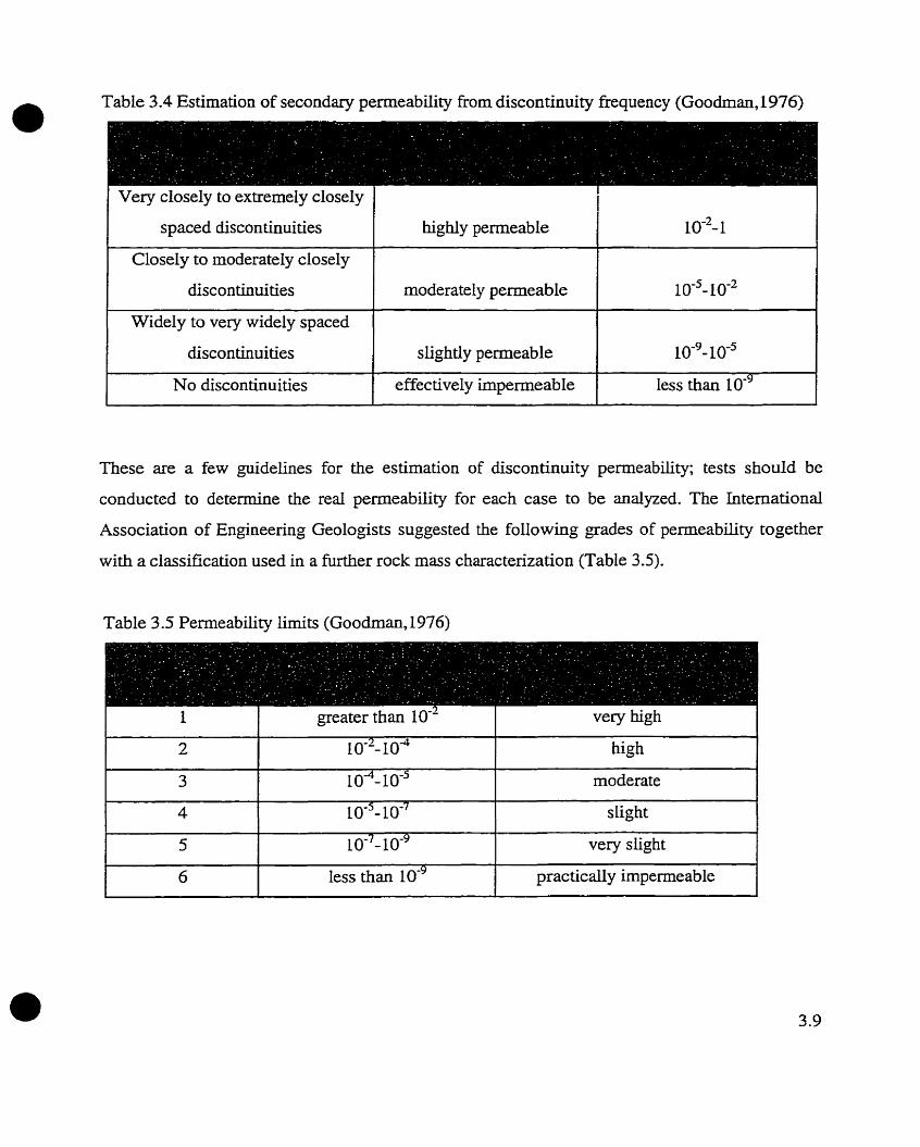
( Very closely to extremely closely i I 1 spaced discontinuities 1 highly permeable 1 1 o-~- 1 I 1 Closely to moderately closely 1 I I I discontinuities 1 rnoderately permeable

These are a few guidelines for the estimation of discontinuity permeability; tests should be

conducted to determine the real permeability for each case to be analyzed. The International

Association of Engineering Geologists suggested the following grades of permeability together

with a classification used in a further rock mass characterization (Table 3.5).

1 0-5- 10-2

Widely to very widely spaced

discontinuities

No discontinuities

Table 3.5 Permeability limits (Goodman,l976)

slightly permeable

effec tively impermeable

l 6 I less than 10" 1 practicaliy impermeable I

1 O-'- 1 o9 less than IO-'

1

2

3

4

5

greater than IO-'

i O-'- 1 o4 I O ~ - ~ O - ~

10"- 10'~

10-7- 1 o - ~

very high

high

moderate

slight

very slight

Some researchen (Louis, 1976) proposed a rock mass classification taking into account the

discantinuitiesT appearance in the geologic formations. Five disfincf groups have been proposed

for the rock masses with respect to their hydraulic properties (Thiel, 1989):

1. porous media (Figure 3.2a), generally hornogenous, containing only smali pores; this group

comprises jointed rock masses which lie at great depth and in which joints have been scaled

by the action of high stresses;

2. porous jointed media (Figure 3.2b), in which discontinuities determine the hydraulic

properties of the rock mass; two types have been distinguished: impervious rock and pervious

rock;

3 . porous media containing impermeable barriers (Figure 3.2c), in which joints are filled

with a fme impervious matenal;

4. porous media with small channels (Figure 3.2d), in which large joints fded with an

impervious material contain channels through which water c a . flow;

5. karstic media (Figure 3.2e) containing wide passages and cavems of various geometricai

forms , created by chernical reaction between water and rock or by removal of the rock in

underground-

l= rock bridge 2= channel

Figure 3.2 Types of media occumng in rock masses (Louis, 1976)

Ali parameters regarding the rock masses and the discontinuities are taken into account in

establishing the model used for solving groundwater fiow. Depending on the desired level of

accuracy, they are going to be either estimated or measured in field andlor lab test. The

estimation of the hydrauIic conductivity with a degree of accuracy could be crucial in further

s tudies.

3.4 Models in hvdrogeologv

Hydrogeology is a relatively new field at the border between rock mechanics and geology. It

deals with problems related to groundwater flow, coupied groundwater flow and stress analysis,

determination of the hydraulic properties of the medium, test and data prediction, well recovery,

dewatering systems and groundwarer contamination problems. In solving these problems,

different types of models were adopted for such studies. It is practicaliy impossible to solve al l

these complex problems taking in account al.€ the parameters existing in nature.

When choosing one model over another, one takes the scale of the analysis of each study into

account. There are no strict rules in doing so, and the analyst should decide what is best for the

study.

When considering the flow of water in jointed rock masses, two major points have to be

considered regarding this phenornenon; models for the medium and models for the flow. Later,

the method to resolve the system of equation could be chosen. Models regarding fiactured rock

medium could be divided in continuous and discontinuous models, each of them with some other

subdivisions. Each model could be applied depending on the degree of fracturing, on avdable

data and on the accuracy of the snidy. Groundwater fiow equations could be solved in different

ways, using analytical methods, numerical methods or analog methods.

In the literature, there are two classes of hydrogeologicai models: one for the network of

fractures and the other for the flow description. The network of fractures could be regarded as

continuum or discontinuum models. The main ciifference between them is the method used to

simulate the fractured media and whether or not an equivalent continuum c m be defmed.

When relating the real network of fractures with the model used for flow, there are two major

concerns: understanding the fracture network with correct representation, and deciding whether

the fractures are suitable for that type of anaiysis. These two have to work together in order to

obtain good results.

In the early stages of hydrogeology, most of the work was focused on generating an equivalent

medium having the equivalent properties of the rock and the fractures together. As a first

defintion, this assumption does not take in account the location of the fractures or their real

peometry. The main goal is to defme an equivalent porous medium.

If it is possible to do so, then it should be possible to determine the representative elementd

volume (REV in the fractured medium), as mentioned herein. In fractured media, there is much

less ceaainty in the assumption of a representative elernental volume being valid (Schwartz and

Smith, 1987). In fractured rock masses, REV could oniy be sampled when the fracture density is

above the critical density. The latter is defmed as the density of fractures that provides the

network comectivity. Below the critical density, the network is not connected and the mean

hydraulic conductivity will be zero, no matter how large REV is (Sahimi,1995).

Fractured rock c m behave as a porous medium when the fractured density increases; apertures

are constant rather than distributed over a large range of values; orientations are more distnbuted

than constant, and a large scale analysis is performed. These conditions satisfied it may be

possible to find a mean value for the equivalent medium.

Long et al. (1982) summarized the conditions that have to be met for a fractured rock to behave @ as a continuum. These are:

1. An insipikant change in the value of the equivalent permeability with a smaü addition or

substraction of the test volume;

2. The existence of an equivalent permeability tensor predicting the correct flux when the

direction of a constant gradient is changed.

The equivalent medium under these conditions behaves like a porous medium. Groundwater

problems could be solved using the classical equations for different types of flow in soi1

material.

In addition , another model for the fractured rock which was formulated in 1960 by Barenbalatt

et al. (1960): the double-porosity model. In their model, the fractured rock is considered as

consisting of two porous systems: the rock matrix with high porosity and low permeabiiity, and

the fractures, with low porosity and high permeabiiity, aiiowing an exchange of fluids between

the systems at their interfaces. In the conceptual model for the double-porosity aquifer, the

porous matrix blocks are assumed to act as sources which feed the fractures.

By using the conceptual framework of a double-porosity medium, three alternative flow models

have been developed. The most siwcant difference among the various models is the treatment

of rock matrïx versus fracture leakage.

Later, Warren and Root (1963) proposed an idealization of the original double-porosity model,

where the fractured rock is represented as regular, fully connected network, embedded in a

porous matrix represented by parallelepiped blocks. Bringing this limitation to the initial model,

some parameters could be estimated from matrix propeaies, like the size and shape of the

blocks. Lïmiting the network of fractures at a uniform distribution through the system, Kazemi

et al. (1970, 1976) proposed methods for estimating various parameters.

a The naturally fractured rocks are very difficult to mode1 with the above mentioned approach,

because they have complex morphological properties such as incomplete fracture comectivity,

fracture surface roughness, and fractal characteristics over certain length scales. There are many

unanswered questions in hydrogeology and without a considerable arnount of assumptions, none

of the real rock mass behavior could be studied.

There are techniques to investigate the geometry of the fracture network: statisticai analysis of

the field data, geophysical techniques for seeing into the rock, and prediction of the fracture

patterns (Witherspoon and Long, 1987). Sirnulating the fracture network could lead to rnodeling

the flow in a discrete manner. In a two-dimension fracture network, rock discontinuity is

represented by one dimensional finite line segment (Lung, 1987) and in three dimensionai

fracture networks, fractures are represented either by discs of finite radii (Dershowitz, 1987) or by

Bat planes of finite dimensions.

New techniques me simulated annealing and synthetic mode1 (Bolton et al., 1987) are used to

generate the network of fractures. These two techniques are applied where classical rnethods

could not be applied; they involve a large arnount of data generated and used .

The methods used for simulating the network of fractures should be cornbined with the different

types of flow for solving groundwater problems. In the case of equivalent medium, classical flow

equations for flow in porous media should be used. Discrete models have the choice over the

flow in a single fracture or between paralle1 plates. Continuity equation is different for each type

of flow; it combines parameters describing the flow and the media Resolving the system of

equations raises another kind of problem.

Over the years, methods for solving groundwater flow problems have been developed.

Depending on type of study and its complexig, one can choose one of the following methods in

resolving the system of equations:

1. Analytical methods;

2. Methods based on the use of models and anaiogs;

3. Numerical methods.

Each of these could be applied depending on the probiem, on the human resource availability, on

the tirne and cost required for reaching a solution. One should take into account the objectives of

the investigation and how the resuIts are going to be used for further studies

The conclusions of this chapter are summarized in the foilowing flowchart, which reviews

different types of models used in hydrogeolo~.

(E-

Double-porositv model for flow in fractured rocks

4.1 Introduction

Flow in fractured rocks is a complex phenornenon, and severai continuum, and discontinuum

models have been developed for studying it. Different studies, that depend on study scaie and

data avaiiable, showed their applicability to e n g i n e e ~ g problerns.

In the mining industry, water flow is important in slope stability studies of open pit mines.

Building high water pressure could favor and induce slope failure. On the other hand, tailings

dams which are made out of mine waste, ailow water to flow freely, affecting their stability. The

two processes are totaliy different, because of the media through which water flows; one is a

naturally fractured slope and the other is a man-made structure out of granular matenal.

Seepage in fractured dope walls of open pit mines has become of more and more concem. The

lack of detailed data describing the network of fractures, as well as the large scaie of the study,

could favor the application of certain models, Like the double-porosity model, which is presented

in this chapter.

In general, fracnired media may be regarded as two coexisting systems of voids: the aperture of

the fractures and the porosity of the blocks of rock separating the fractures. In 1974, Louis,

established some formulations for the equivalent permeabiiity of fractured media in which the

existence of the double system was pointed out. The hydraulic conductivity of the blocks is

added to that of the fractures. That way, different formulations for the ensemble block-kacture

hydraulic conductivity are deveioped (Louis,19'74). Fractures netwoik could be continuous or

discontinuous depending on the connectivity of the discontinuities.

e For continuous fractures: K =-K, +Km;

b

where: e = average aperture of the set of fractures &];

b = mean distance between fractures in the set &] ;

Km = hydraulic conductivity of the rock ma& [Ln] ;

Kr= average hydraulic conductivity of the fractures @l'ï].

I l 1 For discontinuous fractures: K = K + [l + -(- - -)] ; m 2 ( L - i ) L

where: K = hydraulic conductivity in the direction of discontinuous fractures &/Tl;

Km = hydraulic conductivity of rock matrix &/Tl;

L = average distance between (center) fractures [LI;

1 = mean extension of the fractures ( order of 10-') &].

For large scale problems (in tems of special dimensions) the two-media approach of the "far

field mode!" may be used. The conceptualization of the two-media approach, origuially proposed

by Barenblatt et al. (I960), is also known as the 'overlapping continua'. 'double continuum', or

'double-porosity' approach. In this concepnial model, the fractured porous medium is

represented by two distinct, but interacting systems, one consisting of fracture network and the

other, of porous blocks. Each system is visualized as a continuum occupying the entire

investigated domain. Interaction phenomena between the two continua are included to account

for the exchange of fluid between fractures and porous blocks. Since the definition of two

continua is required, one for porous blocks and one for fracture network, it foilows that the

application of the mode1 assumes the existence of a Representative Element of Volume (REV)

4.2

for the fractures and also for the porous medium ( as defmed in the 'previous chapters). But, in the

definition of REV for both systems a common plateau rhould be identifieci, rneaning the

'overlap' of the 'plateaus' defining the REV, and the behavior of the two can be studied together.

The representation of the ensemble is shown in Figure 4.1.

Fractures

I

Figure 4.1 Definition of representative elementary volumes for the fractures and porous block

domain @car J. and B. Berkowitz, 1987)

4.3 Flow velocity

Considering that fractured porous medium consists of a system of porous rock blocks separated

one h m another by fissures with irregular shapes. The elementai macrovoIume, that is a large

volume comparable to the size of an individual block has to be define. This means that the study

domain is much targer than the block size. Furthemore, the size of the block is much larger than

the size of the pores.

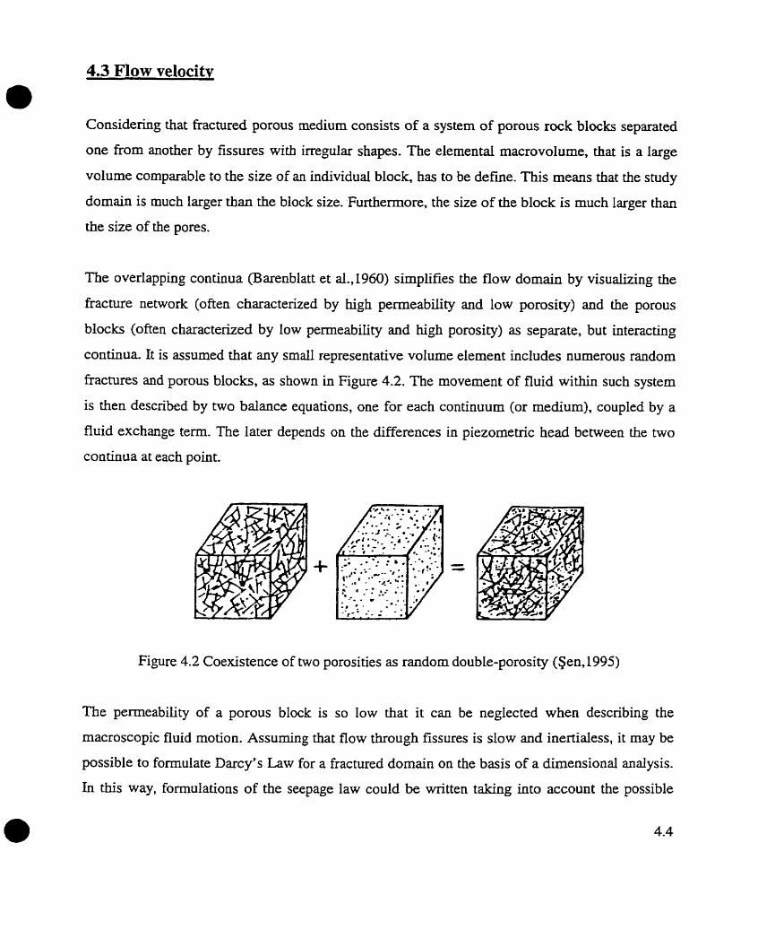
The overlapping continua (Barenblatt et a1.,1960) simplifies the flow domain by visualizing the

fracture network (often characterized by high permeabiiity and low porosity) and the porous

blocks (often characterized by low permeabiiicy and high porosity) a s separate, but interacting

continua. It is assumed that any small representative volume element includes numerous random

fkactures and porous blocks, as shown in Figure 4.2. The rnovement of fluid withùi such system

is then descnbed by two balance equations, one for each continuum (or medium), coupled by a

fluid exchange term. The later depends on the ciifferences in piezometric head between the two

continua at each point.

Figure 4.2 Coexistence of two porosities as random double-porosity (Sen, 1995)

The pemieability of a porous block is so low that it c m be neglected when describing the

macroscopic nuid motion. Assuming that flow through fissures is slow and inertialess, it may be

possible to formulate Darcy's Law for a fractured domain on the ba i s of a dimensional analysis.

In this way, formulations of the seepage law could be written taking into account the possible

anisotropy of fissured systern, and fractures' geometrical characteristics. This Iaw is defined as

(Barenblatt et ai.,1990):

where: Ui = components of flow velocity vector ml; k = fissure permeabiiity tensor [tensor];

h = mean fissure opening &];

2 = characteristic length size of a block [LI;

p = viscosity of the fluid FI/LT];

p = pressure TL?] ;

a = index for each fracture of the set.

The specific form of dimensionless permeability tensor may be determined by the geometry of

the fissure system for a medium consisting of impermeable blocks and several systems of flat and

regularly arranged fissures. It can be evaluated using Boussinesq's formula for the laminar flow

of a viscous fluid through a narrow gap between parae l walls.

In some cases, it is difficult to determine the components of kacture permeabiiity tensor through

calculations. In such situations, experimental data should be used in order to accurately

detexmine the components of the hydraulic conductivity tensor. By choosing properly the systern

of coordinates or by using tensor transformation operations, the hydrauLic conductivity tensor can

be transformed into its principal axes. However, if the pressure gradient is directed dong a

principal axis, flow velocity should have the same direction.

4.4 Flow in fractured media

To establish the basic equations for flow in fractured media, and iater, the double-porosity

equations, a senes of conditions muse be met:

porous blocks are considered impermeable, and their permeability is neglected;

the boundary of a fractured porous reservoir has the initial fluid pressure Po and the pressure

drops to a lower value Pl ;

fluid motion through the fissures can be described with classicd relations of flow theory

through porous media;

after transient process has occurred, a new steady-state distribution of pressure is established

in fissures and, at any place close to reservoir boundary, the pressure WU be considerably

lower than the initial pressure;

as a result of blocks impermeability and of the fact that their pressure could not be changed, a

significant pressure difference will be set up between the fluid in blocks and the fluid in

fissures; (in the order of (Po-PI));

local pressure gradients (Po-Pi)A wiii be created in blocks, and these will be considerably

higher than the pressure gradient in reservoir's fissures which is in order of (Po-P$L.

Under these conditions, local flows are produced in the reservoir, even if the blocks have v e q

low permeability. The Buid flows from blocks to fissures and equalizes the local pressures

(blocks and fissures). A schematic representation considered by Barenblatt in its demonstrations

is presented below (Figure 4.3).

Figure 4.3 A fractured porous medium. The low-permeable porous rnatrix is dissected by a

system of high-conductive fractures which have a srna11 storage capacity (Barenblatt, 1990)

Instead considering of having only one fluid pressure at a given point in the medium, it is

consider the existence of two pressures, one in the fissures (pi), and the other, in the pores of the

block (pz). Both pressures are mean pressure values averaged over scdes, sufficiently large

compared to the scale of the blocks, but srnail compared to the size of the flow region. Assuming

that the permeability of the porous rnatrix is very low, it is possible to use Equation (4.3) in order

to determine the flux through the studied area, by substituthg into it pressure in the fissures pl -

The fluid balance equation (conservation of masses) in the fissures as follows (Barenblatt et al..

1990):

where: mi = fissure porosity (the ratio of the fissure volume to the bulk volume of the

medium) [%] ;

p = fluid density m3]; q = arnount of fluid 80w per unit time, from porous blocks to the fissures, per

unit volume of the medium &/TL3];

u = flow velocity tensor [tensor].

It is possible to ignore the seepage flux from the blocks and write the continuity equation for the

blocks as follows (Barenblatt et al., 1990):

where: mz = porosity of blocks (relative to the buik volume of the medium) [%];

q = amount of fluid flow per unit time, ftom porous blocks to the fissures, per unit

volume of the medium m3]; p = fluid density m3].

Thus, the quantity of liquid flowing into the fissures equals the quantity of liquid flowing out of

blocks. However, the volume of fissures in the blocks is considerably smaller than the volume of

pores. Therefore, the influence of fluid pressure in the fissures (pi) on the porosity of blocks can

be disregarded compared to the infiuence of the fluid pressure in pores (pz), and it can be

assumed that (Barenblatt et al., 1990):

where: mz= porosity of blocks (relative to the bulk volume of the medium) [%];

Pcz= coefficient of blocks compressibility.

The fluid flow from the pores into the fissures (per unit tirne), per unit volume of rock has the

following expression:

where: q= fluid fiow fiom pores to fissures [L/TL~ J;

pa-pi = pressure drop between the pores and fissures [MKL];

a= dimensionless characteristic of the fissured rock;

p= viscosity of the fl uid In/YLT].

The fluid is siïghtly compressible, and:

p=po+P 6~

where: p = density of fluid m3]; po = density of fluid at the standard pressure w3]; p = coefficient of compressibility of the fluid;

6p = change in pressure relative to the standard pressure.

Cornbining the last two equations and neglecting the terms of higher order, the following

equation is obtained:

Assuming that the medium is homogenous and neglecting the smaller higher order terrns:

Furthemore, eliminating pz fiom these equations, the following equation is obtained for the

pressure of the fluid in the fissure Pr:

where: x =coefficient of piezo-conductivity of the fissured rock (it corresponds to the

porosity and compressibility of the blocks);

q = coefficient which tends to O ( corresponds to a reduction in block dimension and an

increase in degree of fissuring)

This equation wiii tend to coincide with the ordinary equation of seepage under deformable

conditions. The above equations describe the motion of a uniform fluid in a fractured rock in the

geeneeral case. Models like double-porosity, start fiom these equations and go further in modeling

the parameters needed for solving the equations.

4.5 The double-porositv mode1

For the motion of homogenous fluids in double-porosity medium, two types of media are

considered (Figure 4.3):

1. porous medium, consisting of relatively wide pores of first order, fissures and blocks (first

order porosity is equai to mi);

2. porous blocks themselves separated by frne pores of second order (second order porosity is

equal to m).

The equations for fluid mass conservation for both media are as (4.4) and (4.5). Assurning that

the flow in both media is inertialess, and Darcy's Law can be written as:

k2 grad p, k lgradp , and u2=-- u1= -- P CL

where: ul and u2= components of the velocity vector for the two media considered V I ; ki and kz= porosities of the system of pores of first order and second order [%];

p= fluid viscosity ( M/LT]-

Assurning that both increments in porosity are linear functions and that they depend on fracture

pressures, it would be possible to wnte their expressions as follows:

and

Inserting the relation (4.12) into Equations (4.4) and (4.5) will give a system of equations similar

to that of heat transfer in a homogenous medium:

where: ml0 and rn?o = values of the frrst and the second order porosity at standard pressure

(Ehrenblatt et a1.,1960).

It is advisable to consider the double-porosity mode1 for a medium in which the porosity of each

order discontinuities depends only on the appropriate pressure. Therefore, P. and P.. coefficients

in Equation (4.13) c m be considered srnall, and the appropnate ternis in Equation (4.14) can be

disregarded. With these assumptions, Equation (4.14) will take a form similar to heat transfer:

Disregardhg the terms in Equation (4.14) representing a change in liquid mass due to

compressibiüty of the £ k t medium and the compression of the liquid in the first order pores, as

weil as the change in liquid mass as a result of seepage inflow dong the pores of the second

order, the same Equation (4.15) of fluid motion in a fissured medium is obtained.

To resolve the last equation, sorne boundary-values must be set up for each case. Methods to

solve this system of equations Vary but are available. Numencd methods are widely used in this

rype of problems. In some cases, the convergence of the solution is not obvious, but it c m be

achieved after considering series of iterations or more assumptions should be considered.

Chapter 5

FlowD finite element code

5.1 Flow equations - analvticai formulations

Based of the formulations of the double-porosity model, the author tned to develop a simple and

practical unite element model to determine flow nets in rock media such as open pit rock slopes.

Flow in fiactured rock slopes becomes very complicated when dealing with large scde studies.

Different orientations of sets of fractures, as well as their hydrauiic properties must be carefully

detemiined. On the other hand, due to the lack of in-situ testing, hydraulic parameters have to be

estirnated from pubiished data.

In this model, presented herein, as a first step in the developrnent of finite elernent code, we have

considered the foLlowing:

steady-state flow conditions;

no fluid exchange between fractures and blocks;

heavily jointed rock with sets of fractures identified as controlLing groundwater flow;

frachxes orientation and their hydraulic properties are considered;

rock blocks are considered to have very low permeability, and their hydrauiic conductivity is

nil;

double-porosity or double-conductivity are accounted for by the motion of equivalent

hydraulic conductivity .

The governing differential equation used in formulation of the FlowD code is:

where: H = total head CL];

k, = hydraulic conductivity in the x - direction WT];

k, = hydraulic conductivity in the z - direction IUT];

Q = applied boundary conditions b3/~].

Under steady-state conditions, the flux entering and leaving an element volume is the same al1

the tirne. In this particular case, the global system of coordinates is important not only in defining

the mesh but also in the formulation of the hydraulic conductivity tensor which differentiates

between the soil material and the rock mass domain.

Hydraulic conductivity tensor is calculated differently for soi1 and rock rnaterials. For soi1 it takes

into account directional hydraulic conductivity in x and z direction for each material, and the

angle between the directionai hydraulic conductivity and the systern of coordinates (Figure 5.1).

Figure 5.1 Hydrauiic conductivity direction for soil material

Far the rock version of the cornputer code, hydraulic conductivity tensor for fiactured rock has

been calculated as a summation of tensors representing hydraulic conductivity of each set of

fractures taking in account their hydraulic properties. This concept was for the fussr t h e

formulated by Feuga (198 1) and is as follows (de Marsily, 1986):

where: K = hydraulic conductivity tensor;

1 = arbitrary dimension of the side of a square block of the fractured medium, large

enough to statisticaliy sarnple al1 the families of fractures IL];

N = number of fractures in the block of side 1;

ei = the aperture of each individuai fracture CL]; k = hydraulic conductivity of each individual fracture [ Lm] ;

Ri = matrut depending on the direction d and the dip of each fracture, its form WU be

presented in the next chapter.

The matrix Ri has the following f o m for each set of fractures:

1 1 1 -cos2 di sin' pi -sin2di sinZpi --sin2pi cosdi

2 2 1 1

-sin 2di sin' pi 1 - sin' di sin2 pi -sin2pi sind, 2 2

1 1 --sin 2pi cosd, -sin 2p, sind,

2 2 sin' pi

where: di = direction of the set i of fractures [degree];

pi = dip of the set i of fractures [degree].

The total hydraulic conductivity vector K is rotated in the plane of the snidied cross section, after

which is extrapolated for a 2D analysis. For the FIowD code, the global system of coordinates is

represented in Figure 5.2. The Oy axis represents also the North direction and the analysis is

performed in the xOz plane, which is practicdy the plane of a vertical cross section in a slope.

Figure 5.2 Global system of coordinates for the hydraulic conductivity tensor(de Marsily, 1986)

Blocks are considered practicaily impermeable and flow takes place mostly in fractures. Their

orientation becomes very important in studying 80w. It is difficult to approximate the hydraulic

properties of fractures when field tests do not exist. But, dealing with large scde studies, where

fractures' orientations are available and the rock properties are known, assumptions regarding

their hydraulic properties can be estimated from Literature.

5.2 The auadrilateral isoparametric element

Finite eIernent method has often been applied in solving groundwater flow problems. The f ~ t e

element mesh in this case, employs 4-node isoparametric elements represented in Figure 5.3 with

their local system of coordinates (s, t). The gIobal coordinates (x, z) of any point in the element

are reIated to the local coordinates (s, t) through the foLlowing equations:

where c N > is an array of interpolating shape functions and { X ) as weil as { Z ) are the global

x, z coordinates of the element nodes. The shape functions are expressed in terms of local

coordinates and have the following form for the 4 - nodes isoparametrk element:

Figure 5.3 Isoparametric Cnode element in the global and local system of coordinates

In order to formuiate the finite element equations, it is necessary to adopt a mode1 for the field

variable within the element. In the seepage analysis, the field variable is the total head (H) and a

model has to be adopted for its variation within the element. FlowD code considers that the total

head distribution within the element follows the interpolating functions presented above, which

means that the head distrfiution is linear- The distribution of the total head in the element could

be summarized by the following equation:

where: h = head at any point;

< N > = array shape fünctions;

(H) = vector of heads at the nodes.

The constitutive law for the seepage analysis is Darcy's Law previously presented. For FlowD

code this law is expressed by the conventional equation:

where: q = groundwater flux P T ] ;

k = hydraulic conduc tivity [UT] ;

h = gradient [UL] .

In the f ~ t e element formulation, the hydraulic gradient 'i' is a key parameter. The procedure

used in the FlowD code to compute the gradient is presented below.

The gradients in x and z direction are:

The shape fûnctions are given in terms of local coordinates s and t, and must be computed in

terms of the global coordinates. In this case, the derivatives must be determined by the chah rule

of differentiation as foliows:

W c h can be written as:

where: [JI is the Iacobian matrix. Performing

interpolating function with respect to x and z c m be

matrix operations, the derivative of the

detennined, and the equation is rewritten as :

AU the above vectors will be used in the finite element formulations of the seepage equations.

The hydraulic gradient in ma& form cm be written as:

where: [BI= characteristic gradient matrix;

[JJ- gradient vector;

CH)= hydraulic head vector = < Hl, H2, Hg, &>.

5.3 Finite element formulation

The f i t e element equation chosen for the seepage analysis performed by the FlowD code results

from the application of the Galerkin method of weighed residuals to the governing differential

equation (5.1), and is given by:

where: [BI = characteristic gradient matrix,

[Cl = elernent hydraulic conductivity matrix;

{H) = vector of nodal heads;

q = unit flux across the side of an elernent;

< N > = vector of the shape functions.

For the two-dimensional analysis, the thickness of the element is considered to be constant over

the entire domain. The fuiite element equation could be written as :

where t is the element thickness. The abbreviated form of the element equation is:

where : [KIe = element charactenstic matrix;

{Hle= vector of nodal head;

{QIe= applied flux vector.

Special attention is given to the element characteristic ma&. For soi1 materials the general form

of hydraulic conduc tivity matrix is:

where: CI I= kx* cos' cc+ k, * sin' cx

Czz= k,* sin' a+ k,* cos' a

Clr= kx*cos a s i n a- k,* sin occos a

CZI = CI?

Parameters k,* and k,* correspond to hydraulic conductivity in x* and z* directions; a is the

angle between the system of coordinates (x, z) and the hydraulic conductivity directions (x*, z*)

(Figure 5.1).

In the case of double-porosity mode1 the hydraulic conductivity ma& is determined by taking

into account the sets of fractures with their hydraulic conductivity properties, the average number

of fractures in a set, the average aperture and their spatial orientation as in Equation (5.2).

Extrapolation of the two dimensional characteristics matrix is oeeded in order to formulate the

fractured flow. The projection of the dip and dip direction of the sets of fractures and their

hydraulic properties are needed. The hydraulic conductivity of each set of fracture has to be

positive defmed, the angle between the fractures orientation and the system of coordinates gives

the flow direction.

\ set 2

Figure 5.4 Hydrauiic conductivity of sets of fractures

In order to resolve the system of equations, the boundary conditions must be imposed. RowD

code takes two types of boundary conditions. The fxst one is Dirichlet boundary condition of

specified pressure hezd at a certain node of the mesh; the second one is the Neumann boundary

condition which specifies groundwater flow rate over the side of an elernent or a punctual flux in

a node of the mesh. Pracûcally, Neumann boundary condition is counted as a nodal flux

boundary in the program as follows:

(e) (e) { } N i q dl?

where: Fi = nodal boundary flux;

Ni = shape function for that element;

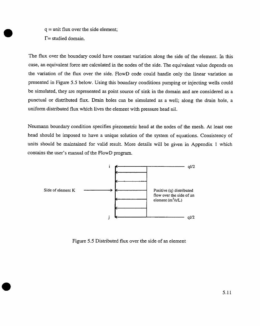
q = unit flux over the side element;

r= studied domain.

The flux over the boundary could have constant variation along the side of the elernent. In this

case, an equivalent force are calculated in the nodes of the side. The equivalent value depends on

the variation of the flux over the side. FlowD code could handle oniy the linear variation as

presented in Figure 5.5 below. Using this boundary conditions pumping or injecting weils could

be simulated, they are represented as point source of sink in the domain and are considered as a

punctual or distributed flux. Drain holes can be sirnulated as a well; along the drain hole, a

uniform distributed flux which lives the element with pressure head nil.

Neumann boundary condition specifies piezometric head at the nodes of the mesh. At least one

head should be imposed to have a unique solution of the system of equations. Consistency of

units should be maintained for valid result. More details will be given in Appendix 1 which

contains the user's manual of the FlowD program.

Side of eIement K - Positive (q) distributed flow over the side of an elernent (m3/s/~)

Figure 5.5 Distributed flux over the side of an element

5.4 Equation solver

FlowD uses Choleski decomposition technique to solve the finite element system of equations.

The objective of solving the finite element equations is to compute total head at each node. The

equations are hea r , as being the assumption of steady state flow is made. Figure 5.6 presents the

numencal integration scheme used and the d e f ~ t i o n of the element parameters.

Numerical integration scheme Defini t ion of element parameters

Figure 5.6 Numencal integration scheme

Once the equations are solved, the nodal heads are known, FlowD computes the hydrauLic

gradients and the Darcian velocities at the center of each element, using Equation (5.1 1). The

Darcian velocities are calculated as follows:

In the output file, the hydraulic head is specified at each node of the mesh and hydraulic gradients

and hydraulic velocities, at the center of each element.

5.5 FIowD computer code

FiowD computer code is a finite elemeat program that performs two-dimensional confined

steady-state seepage andysis, homogenous or nonhomogenous soi1 andor rock, and isotropic or

anisotropic media. Boundary conditions are: (1) specified total head at the rnesh boundary nodes,

(2) specified ffow at the mesh nodes. Nonhomogenous media are handled by aliowing zones or

elements to have diEerent materiai properties, and the anisotropy is modeied by using the general

2x2 hydraulic conductivity tensor in the expression of Darcy's Law. A speciai treatrnent is given

to the hydraulic conductivity tensor when the double porosity mode1 is applied, sets of fractures

are considered in the modeling process and their orientation and spacing modify the formulation

of this tensor.

The code employs 4-node isoparametric elements with 2x2 Gauss integration scheme and is

written in FORTRAN 77. To solve the equation system, a banded technique is used. The mesh is

generated automaticaiIy, using an in-house mesh generator developed at the Numerical Modeling

Laboratory of McGill University.

The computer program calculates velocities, hydraulic gradients and total heads at the nodes.

Figure 5.7 presents the flowchart of the program .

Set boundary conditions CALL BOUND

identify degrees of freedom CALL IDJD

I

*.DAT Start prograrn FIowD

I ".HED

* I I = f , NEL

Build element connectivity array CALL ELCON

CALL BANDWH

Compute load vector CALL LOAD

Mesh generator

I 1 - 1 , NEL

-+( '.COR

1 1 Compute characteristics matrix 1

CALL CARASO

For soi1 mode1 t I

I

I CALL IPLNCF I 1 rn For double-porosity rnodel

Modify load vector 1

Prepare banded matrix CALL ELCON

1 CALL SETUP2 1 l

Solve system of equations by Cholesky decomposition

CALL CHLSKI

CALL DPOR

Calculate gradients and velocities CALL GRADIE

Prepare output file

Figure 5.7 Flowchart of the FlowD coc

The computer code could perform seepage analysis in the horizontal and vertical plane

depending on the section studied. Figure 5.8 shows two types of analysis that FlowD can

annualize. The soi1 version of the program has two features for horizontal and vertical cross

section. The double-porosity version of the program has only the vertical cross section option.

Vertical cross section in an open pit slope Regional groundwater flow in an open p i t

Figure 5.8 Types of analysis performed by FlowD

Mode1 verifkation and aoplication

6.1 FlowD code verification

The verifcation of FlowD code and validation were performed on simple examples which were

taken from different reference books. The double-porosity version of the code could not give the

same results as other codes, having a different approach but in most of the cases the results could

be pertinent. Two simple examples were run in order to v e m the soi1 version of the code.

The first one consists of two-dimensional confmed aquifer with two types of matends (silty sand

and sandy gravel) considered isotlopic with the same hydraulic conductivity in both directions;

12 elements mesh was design, with two types of boundary conditions: constant head dong one

edge of the rnesh and a discharge well situated in one of the mesh nodes. This example was taken

from the book by Istok J. (1989, page 259). The results of the RowD code were very close to the

ones specified in the reference. The margin of error was lower than 0.01%.

The second test of the code was seepage anaiysis under a dam. The dam itself was considered

impermeable and its foundation was assumed to be layered. Just the constant head boundary

condition was irnposed. The two materials were considered anisotropic, with different horizontal

and v e r t i d hydraulic conductivity (U30 and 1/25). The solutions were verified manually, giving

a difference of 0.01% fkom the code calculation.

Some other verifications were performed iike mesh density analysis, but they are not descnbed

here. From the verification process it can be concluded that the cornputer code gives accurate

results for the total head, hydraulic gradients and 80w velocities, in such type of analysis.

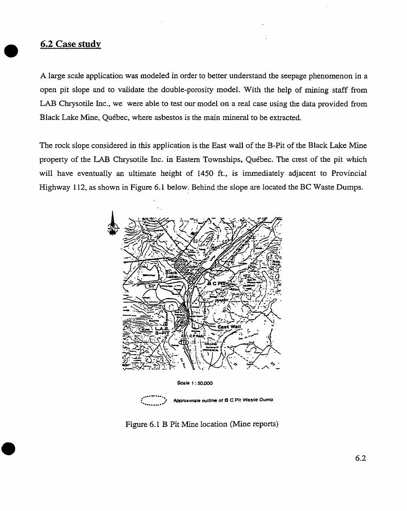
6.2 Case studv

A large scale application was modeled in order to better understand the seepage phenomenon in a

open pit slope and to validate the double-porosity model. With the help of mining staff fiom

LAB Chrysotile Inc., we were able to test Our model on a real case using the data provided fiom

Black Lake Mine, Queoec, where asbestos is the main d e r a l to be extracted.

The rock siope considered in this application is the East wall of the B-Pit of the Black Lake Mine

property of the LAB Chrysotile Inc. in Eastern Townships, Québec. The crest of the pit which

will have eventually an ultimate height of 1450 ft., is immediately adjacent to Provincial

Highway 112, as shown in Figure 6.1 below. Behind the slope are located the BC Waste Durnps.

Figure 6.1 B Pit Mine location (Mine reports)

During mining operation, the desiga of the B Pit east waii was modified according to different

engineering design studies, behavior of the slope, slope stability, water pressure in the waU and

slope response to mining activity. Since the beginning of the mine the Highway 112 was

relocated in order to expand the rnining activity in a safety way and to better monitor slope

stabiiity.

6.2.1 East wail of Black Lake Mine

The original design for the slope was based on an overail angle of 45" for the initial cut, followed

by a 600 fi. pushback to the ulùnate, which will have a multiple angle slope, graduaily flattening

with depth. This design was changed during mining operations.

The general geology of the B Pit refiects the existence of three major rock types: massive,

unaltered or weakly serpentinized peridotite; semi-schistose or schistose serpentinite (totally

altered peridotite), and talc-carbonate shear zone. Narrow granitic veins occur through the wall;

these are typically up to 10 ft. thick and strike down in the wall parailel to the regional structure

(Figure 6.2).

From the hydrogeological point of view the high water table in the slope, the poor drainage

performance and high groundwater recharge h m the east through the BC Mine dumps rise more

concems about the real seepage phenomenon in the slope. During the years of operation,

intensive studies were conducted for a better understanding of water flow phenomenon in the

slope. Two pumping tests, one in the massive pendotite and the other in the schistos serpentinite

were performed. Monitoring piezometers were installed in the crest of the ultimate pit. Inclined

drain holes were drilled for depresurization. Different other methods of mine dewatering were

studied, as pumping wells system or the design of an infiltration gallery in the slope.

Figure 6.2 B Pit Mine geological plan view ('Mme reports).

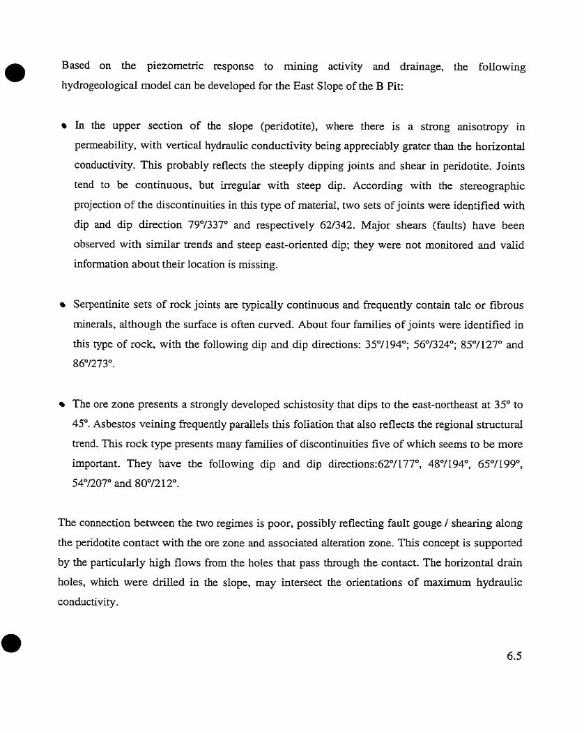
Based on the piezometric response to rnining activity and drainage, the following

hydrogeologicd mode1 can be developed for the East Slope of the B Pit:

In the upper section of the slope (peridotite), where there is a strong anisotropy in

permeability, with vertical hydraulic conductivity being appreciably gaier than the horizontal

conductivity. This probably reflects the steeply dipping joints and shear in peridotite. Joints

tend to be continuous, but irregular with steep dip. According with the stereographic

projection of the discontinuities in this type of material, two sets of joints were identified with

dip and dip direction 7g01337" and respectively 621342. Major shears (faults) have been

observed with similar trends and steep east-oriented clip; fhey were not monitored and valid

information about their location is rnissing.

Serpentinite sets of rock joints are typically continuous and frequently contain talc or fibrous

minerais, although the surface is often curved. About four families of joints were identified in

this type of rock, with the following dip and dip directions: 35"/194"; 56"/324O; 85"/127" and

86"/273".

The ore zone presents a strongly developed schistosity that dips to the est-northeast at 35" to

45". Asbestos veining frequently paraiieIs this foliation that also reflects the regional structural

trend. This rock type presents many families of discontinuities five of which seems to be more

important. They have the following dip and dip directions:62O/ 177". 48'1 194O, 6S0/ 19g0,

54"/207" and 80°/2 12".

The comection between the two regimes is poor, possibly reflecting fault gouge / shearing dong

the pendotite contact with the ore zone and associated alteration zone. This concept is supported

by the particularly high flows from the holes that pass through the contact. The horizontal drain

holes, which were W e d in the slope, may intersect the orientations of maximum hydraulic

conductivity .

Depresurization of the slope was needed in order to lower the water table and to drop the water

pressure. Holes were drilled dong the entke length of the wail, dthough there should be

concentration in the areas of highest flows. A general spacing of 150 ft. dong the wail on every

second bench is recommended, with the spacing reduced to 50 ft. at the holes ends where the

peridotite, schistose serpentinite contact is intersected. Installation of piezometers for monitoring

the water pressure level was performed. Their location is dong the highway at 1000 fi. intervals

dong the crest of the wall.

For a better depressurization of the pit walk pumping wells installation solution was studied. In

the area of schistuosity associated with the ore zones, it should be possible to achieve deeper

depresurization with vertical wells, which would be most suitable drilled fiom the proposed ramp

on the ultirnate wall. An other method of depresurization considered by the consultant was the

design of a drainage gallery in the slope which will collect the same amount of water as the

pumping weUs system.

6.2.2 Slope geometry and hydrogeological regime

A typical cross section in this wall was chosen for the anaiysis. The height of the slope was

458m. with an overall angle of 27". In the slope, three types of materials, were identifïed, and

their charactenstics follow the tests performed d u ~ g the operation years.

The geornetry of the dope is shown in Figure 6.4. Because of the recharge from the waste dumps,

water table elevation is very high and was considered to be at the face of the slope. The two

piezometers instded from the upper bench confinned this fact and also indicate high water

pressure in the wall. The geology consists in massif peridotite rock in the upper p m in where two

families of fractures are predominant. The sarne type of rock was found in the lower part closed

to the toe of the slope. The ore body dips down east in the slope with an angle of 27" fiom the

vertical. This part is highly fiactured, having the discontinuities filled with fine matenal. Five

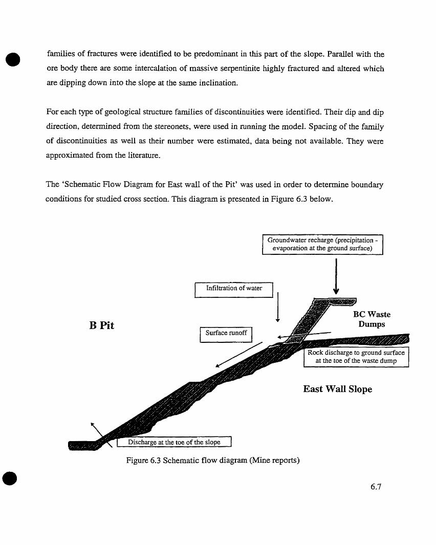
a families of fractures were identified to be predominant in this part of the slope. Parallel with the

ore body there are some intercalation of massive serpentinite highly fractured and altered which

are dipping down into the slope at the same inclination.

For each type of geologicd structure famiLies of discontinuities were identified. Their dip and dip

direction, determined fiom the stereonets, were used in running the model. Spacing of the family

of discontinuities as well as their number were estimated, data being not available. They were

approximated fiom the Iiterature.

The 'Schematic Flow Diagram for East wali of the Pit' was used in order to determine boundary

conditions for studied cross section. This diagram is presented in Figure 6.3 below.

- 1 Groundwater recharge (precipitation - 1 1 evaporation at the ground surface) (

Infiltration of water I

B Pit

East Wall Slope

Figure 6.3 Schematic f h w diagram (Mine reports)

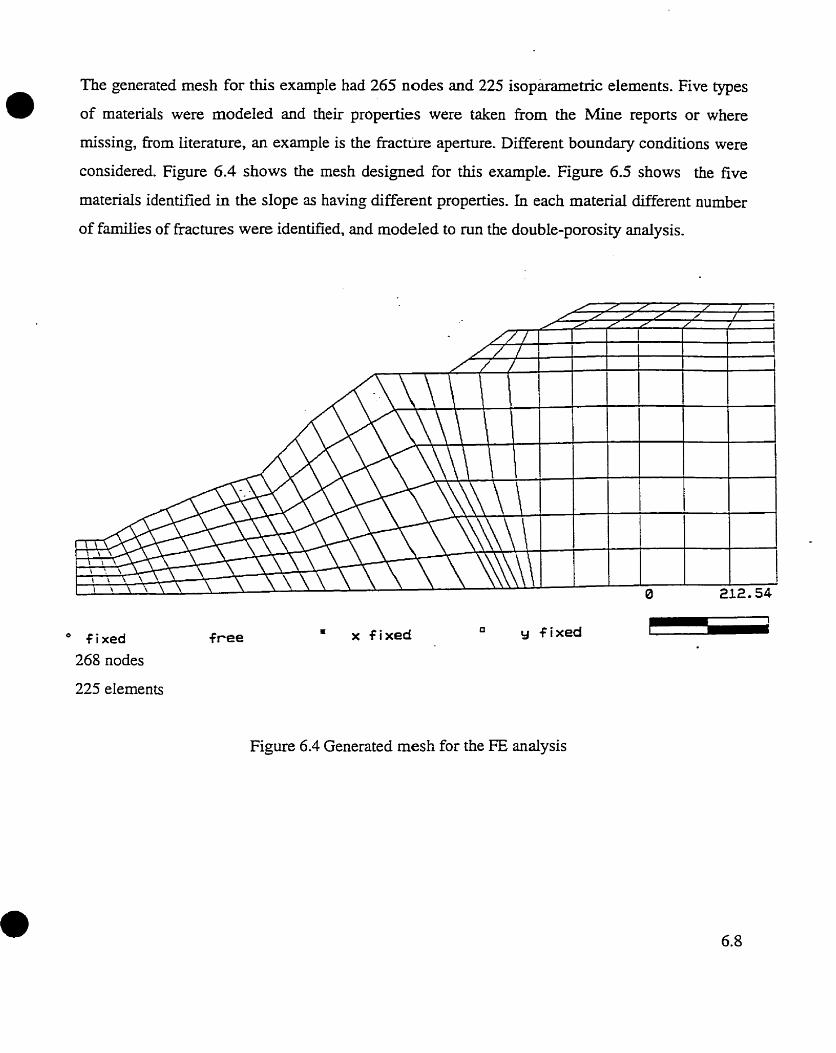
The generated mesh for this

of materials were modeled

example had 265 nodes and 225 isoparametric elements. Five types

and their properties were taken from the Mine reports or where

rnissing, fiom literature, an exarnple is the fracture aperture. Different boundary conditions were

considered. Figure 6.4 shows the mesh designed for this example. Figure 6.5 shows the five

materials identified in the slope as having different properties. In each matenal different number

of famiLies of fractures were identifïed, and modeled to run the double-porosity analysis.

O fixed

268 nodes

225 elements

free * x fixed y fixed

Figure 6.4 Generated rnesh for the FE analysis

RATL

Figure 6.5 Materials identified in the 5000 N Section

In order to determine the water regime in the slope, three models were designed:

Mode1 1: water regime in the slope without any measure of dewatenng, representing the fIow

diagram (Figure 6.3).

Model H: well simulation, as a dewatering option.

Model III: drainage gailery simulation, as a dewatering option.

Running the program for the Model 1 showed that the water regime in the slope present a high

vertical anisotropy with high water pressure that can be explained by very low hydraulic

conductivity of the materïals. The dope zone that is highly fractured, and the fractures orientation

dipping down into the slope practicalIy control the water flow. The permanent recharge of the

slope from the waste dumps and the poor drainage, caused by low hydrauk conductivity of the

materials explain the high water pressure in the wall. Figure 6.6 shows the water velocity vector

in the slope. As it can be seen, the chird material rnodeled drains the entire dope and do not aüow

water to be drain properly from the surface. The equipotential Lines are presented in Figure 6.7.

Velocity vector in the 5000N Section (regional goundwater flow)

Figure 6.6 Groundwater flow velocity

Model II and Model III simulate d e w a t e ~ g methods considered by the Mine. Figure 6.8 and

Figure 6.9 show the total head in the slope and the equipotentid lines surrounding the weil and

the drainage gaileries The low hydraulic conductivity of different materials and the middle highly

fractured formation dipping down in the dope rnake very difficult the process of slope

dewatering. The water pressure decreases, but not in a way that can be satisfactory enough.

Probably, a more complex method of dewatenng or a combination of different rnethods should

be used in order to considerably lower the water pressure in the slope. Free drainage of the dope

could not be possible in such materials because of their properties and irregular intemal

geologicai features.

Figure 6.7 Total head - 5000N Section - Regional growndwater regime

Figure 6.8 Total head - 50ûûN Section - Well simulation

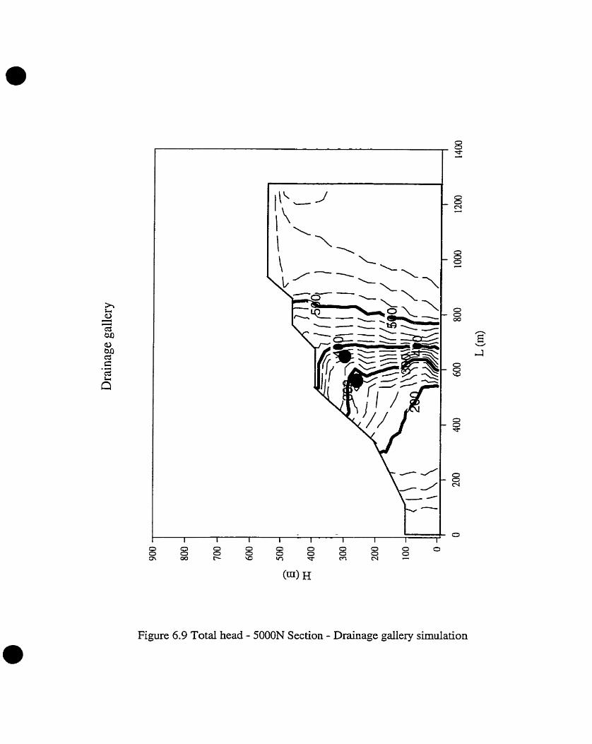
Figure 6.9 Total head - 50ûûN Section - Drainage galiery simulation

Conclusions and recommendations for further research

Open pit slopes have become of more and more interest in geotechnicai engineering for safe and

economic surface mining operations. Stabiiity of these slopes could be infiuenced by different

geological, hydrogeologicd and structural factors. Groundwater regime in high slopes could badly

damage their stability. Rock mass properties changes in contact with water and structural behavior of

any slope changes when groundwater oudlows appear at the face.

These were just a few reasons why the groundwater flow in fkxhu-ed open pit slopes shodd be

determine. Flow in hctured rocks dBers from flow in porous media and, in some cases, traditional

flow equation could not describe the real state of media. Double-porosity model for flow in hctured

rocks could reflect, with a higher grade a confidence, the groundwater regime.

As a k t step in application of the double-porosity flow to large scaie studies in mining industry, the

FlowD finite element code was developed. It is the bais for m e r appiicability of this model to

mining related problems. It perEorms steady-state flow andysis, and calculates total pressure head,

gradients and velocities in the specific section of a slope.

RowD code was initially verifid on soi1 examples where no double-porosity models is applied to this

type of analysis. Later, a study case was conducted on a real mining slope using double-porosity

model. The resdts obtained validate this model showing consistency with actual flow state in that

particular slope, as detennined by monitoring and various other analytical rnethods used by the mine

consultant. In the same t h e , the introduction of fracture orientations and hydraulic properties could

model better the flow regime in the studied slope.

FlowD code performs steady-state seepage analysis in blocky rock slopes in which families of a discontinuities couid be sarnpled and thek pmperties determinecl. It models Dirichlet and Neumann

boundary conditions. Drains, weils and drainage gaileries could be modeled.

FIowD cornputer code codd be integrated in a stressdeformation anaiysis. It can be improved by

adding the determination of the phreatic surface and in this way to mode1 double-porosity unsteady-

state flow in blocky rocks. For an easier way to use it, a pre and post-processors could be added which

can give the user a better filling and ease in anaiyzing large scale problems.

Chapter 8

References

1. Amadei, B. et al., 1995,'Effect of turbulence on fracture flow and advective transport of

solutes', Technical Note, Int. J. of Rock Mech. & Min- Sci. & Geotechnical Abstracts, Vol. 32,

NO 4, p. 342-356.

2. Bai M. et al.,'Fiuid flow and heat flow in deformable fracnired porous media'J994, Int. J.

Engng Sci. Vol. 32,No. 10,pg 1615-1633.

3. Barenblatt, G.I. et al.,' Basic concept in the theory of seepage of hornogenous liquids in

fissured strata' ,1960, Journal of Applied Mathematics and Mechanics, Vol. 24, 1286- 1303.

4. Barenblatt, G.I. et al.,'Theory of fluid flow through naturai rocks'J990, Kluwer Academic

Publis hers.

5. Bear, J. et al.,'Groundwater fow and pollution in fractures rocks aquifers7,1987, Developments

in Hydraulic Engineering - No. 4, Elsvier.

6. Bear, J. et al., 1972,'On the flow of two imiscibile fluids in fiactured porous media', in

Fundarnentals of Transport Phenomenon in Pouous Media, Elsevier.

7. Bear, J. et al., 1993, 'Flow and Contaminant Transport in Fractured Rock', Academic Press

8. Bear, J.,'Modelling flow and contaminant transport in fractured rocks7,1993, Flow and

Contaminant Transpoït in Fractured Rocks, Ed. Bear, J. et ai., Pb. Academic Press.

9. Bear, J., 1979,' Hydraulics of Groundwater7, Pb. Mc Graw - Hill.

10. Bieniawski, Z.T.,1989, 'Engineering Rock Mass Classifications', Pb. John Wiley & Sons.

11- Boca, R.G et al.,'Modelling fluid flow in fiactured-porous rock masses by finite element

techniques', 1984, International Journal for Numericd Methods in Fluids, Vol. 4, pg. 337-348.

12. Brady,B.H.G. et al., 1993,'Rock mechanics foe underground mining9,Chapman & Hall.

13. Chan, T. et al.,'Finite-element simulation of groundwater flow and heat and radionuclide

transport in plutonic rock mass'J987, 6" International Congress in Rock Mechanics,

Proceedings, Ed. Herget, G. et al., Pb. Balkena.

14. Chisbolm, J.S.R.,'Vectors in three-dimensionai space'J978, Cambridge University Press.

15. de Marsily, G.,' Qualitative hydrogeology for engineers' , 1986, Academic Press.

16. Dershowitz, W.S. et al.,'Three dimensiond flow modeling in jointed rock masses', 1987, 6"

International Congress in Rock Mechanics, Proceedings, Ed. Herget, G. et al., Pb. Balkena.

17. Deskowitz, W.S. et al.,' Fracture modelling with IlNX pakage7,1987, 28" US Symposium on

Rock Mechanics, Proceedings, Tucson, June 29" - July lSt, 1987.

18. Fan, Y. et al.,'Generation of fiow netsusing f.e.m. nodal potential and bilinear shape

functions', 1992,Internationa.l Journal for Numerical and Analytical Methods in Geomechanics.

a 19. Feuga, B, 'Modelling of fiow through fractured rocks. Geostatisticd generation of fractured

networks. Stress - flow relationship in fractures.', 1987, Groundwater Flow and Quaiity

Modeiling, Ed. Custodio, E. et al., NATOI AS1 Series.

20. Freeze, A. et al.,'Groundwater', 1979, Pb. Prentice - Hall Inc.

21. Goodmann,'Methods in geologicai engineering in discontinuous rocks', 1976, West

Publishing Company.

22. 'Groundwater Models, Scientific and Regulatory Appiications7,1990, National Research

Concil, National Acadernic Press.

23. Hoek, E. et al.,'Rock slope ena@neeRng',1981,The Institution of Mining and Metaliurgy,

London.

24. Huyakon, P.S. et al., ' Finite Element Technique for Modeliing Groundwater Flow in

Fractured Aquifers', 1983, Water Resources Research, Vol. 19, No 4, p. 10 19- 1035

25. Istok, J.,' Groundwater modehg by the Finite Element MethodY,l989, Water Resources

Monograph, No. 13, American Gephysical Union

26. Kavacs & Associates, 198 1,' Subteran Hydrogeology' , Water Resources Publications.

27. Khaieel, R.,'Scale dependence of continuum models for fractured basalts', l987,Water

Resources Research, Vo1.23,N0.8,pg 1847- 1855.

28. Lee, C.-K. et al., 'Fluid Flow in Discontinous Rocks',1993, Pb. Chapman & Hall.

29. Long,J.C.S. et al.,'Porous media equivalents for networks of fracturesY,l982, Water a Resources Research, Vol. 18. No.3,pg 645-658.

30. Lopez,D. et al.,'Fluid flowin fait zones: Analysis of the interplay of convective circulation

and topographicaliy driven groundwater flow7,i995, Water Resources Researche, Vol.3 1,No.

6,pg 1489-1503.

3 1. Louis, C. et al.,'Interaction between water flow phenornena and the mechanicd gehaviour of

soil or rock masses', 1975,"Finite elements in geomechanics", Ed. Gudehms G.

32. Louis, C.,'Introduction a l'hydraulic des roche', 1974, Bulletin du Bureau de Recherches

Geologiques et Miners, Section III, No. 4.

33. MacQuaime, K.T.B. et al.,'On the interpretation of drains into three-dimentional variably

saturated grounwater flow models', 1996, Water Resources Researche, Vol. 32,No.2, pg 477-

482.

34. Matheson, C.H., Engineering geology', 198 1, Charles E. Merrill Publishiag Company.

35. Minùig Research Laboratoy,'Pit slope manuai', Chapter 4, Groundwater, 1977,CANMET.

36. Mining Research Laboratoy,'Pit slope manual', Cornputer manual for seepage analysis,

supplement 4- 1, 1977,CANMET.

37. Novak, P., 'Developments in Hydraulic Engineering - 4'. 1987, Pb. Elsvier Applied Science.

38. Parkin, G.W. et al.,'Analytical solution for one-dimensionai drainage: Water stored in a fixed

depth', 1995, Water Resources Research, Vol. 3 1, No. 5, pg. 1267- 127 1.

39. Pinder, G.P. et al., 'Simulation of flow and transport in fiactured porous meddia', 1993, Flow

and Contaminant Transport in Fractuied Rocks, Ed. Bear, J. et al., Pb. Academic Press.

40. Pyrak-Nolte,L.J. et aI.,'Hydraulic and mechanical properties of natural fractures in low

penneability rock' 1987, 6" International Congress in Rock Mechanics, Proceedings, Ed. Horget

G. et ai., International Society of Rock Mechanics.

41. Rushton,K.P., 'Groundwater models',l987,in Developments in Hydraulic engineering-

4', 1987, Ed. Novak, Elsevier.

42. RutonJ et aI.,'Multiple seepage faces on layerd slopes and their inplication for slope stability

analysis', 1985, Canadian GeotechrricaI Journal, Vol. 22,pg. 347-356.

43. Sahimi, M.,'Flow and transport in porous media and fractured rocks7,1995, Pb.

Verhageselischaft.

44. Sharp, J-C. et al.,'Fundamental considerations on the hydraulic characteristics of joints in

rock', 1972, Symposium Percolation Throgh Fissured Rock, Proceedings, Ed. Gessllschaft D. and

W. Wittke.

45. Stock, Q.,'Groundwater Mechanics', 1989,Prentice Hail Inc.

46. Sen,Z.,' Applied hydrogeology for scientists and engineers ' ,1995,Lowis Publisher.

47.Themen, R., 1994, 'Kydrogogeology', Course notes, McGill University.

48. Thiel, K, 'Rock Mechanics in Hydroengineering' , 1989, Developments in Geotechnicai

Engineering, Vol. 5 1.

49. Wdton, W.,' Principles of grundwater engineering', 199 1, Lewis Publshers.

50. Wang, H.F.,'Introduction to groundwater modeiling, Finite difference and finite elenent

methods', 1982.

5 1. Wei,Z.Q. et al.,Permeability prediction for jointedrock masses', 1995, Int. J. Rock Mech.

Min. & Geomech. Absu., Vol 32,No. 3, pg 251-261.

52. Witherspoon,P.A. et al.,'Some recent developments in understanding the hydrology of

fractured rocks', 1987,28" US Symposium on Rock Mechanics, Proceedings, Tucson, June 29" - July lSt, 1987.

53. Wittke,W.,'Rock rnechanics, Theory and AppLications',l990, Springer-Verlag Berlin

Heidelberg.

54. Bouchamp,Y.,' Blake Lake Operations', Presentation, November 1994.

55. 'Report to LAI3 CHRISOTLE INC. on a Riview of dope designs for the B Pit East Wall',

1990, Golder Asociates Ltd.

56. 'Interim raport to Lake Asbestos of Quebec Ltd. on A stability review of B Pit East

Wali' ,1978, Golder Asociates Ltd.

57. 'Draft report to Lake Asbestos of Quebec Ltd. on the 178 Stability Pogram for the B Pit East

Wall', 1979, Golder Asociates Ltd.

a Appendix A: User's manual

The present version of the FlowD code mns on IBM compatible cornputer machine equipped with a

mathematicai processor and a hard disk (minimum lOOMB IÏee mernoiy). This £ ï ~ - ~ t version of the

code does not have a rnesh generator. The mesh can be generated with any 2-dimentional mesh

generator for Cnodes isoparameûic elements. The code accepts a maximum of 1OOO nodes.

To run the program, the user has to create two separate hles: one reflecting the nodal coordinates and

the comectivity of the mesh (*.COR), and the other describing specifïed where material properties

and the boundary conditions are specified (*.Hm). The file name has to be the same for *.COR and

*.HED. The program automaticaily search for the same name for both files. Also the program wfl

automatically create the output file with the same name as the *.COR and *.HED. For example: create

file PROGRAM.COR, with boundary conditions in file PROGRAM-HED. Output ille will be

PROGRAM.0UT.

A. Input nle (*.COR and *.EED)

A.1 Data file *.COR (nodes, coordinates and elements)

1. Fit card:

Title of the problern to be solved = no more than 80 characters, including spaces

2. Number of nodes in the mesh,

NNODES= total number of nodes in the mesh (maximum 1000)

User Manual FZowD. 1

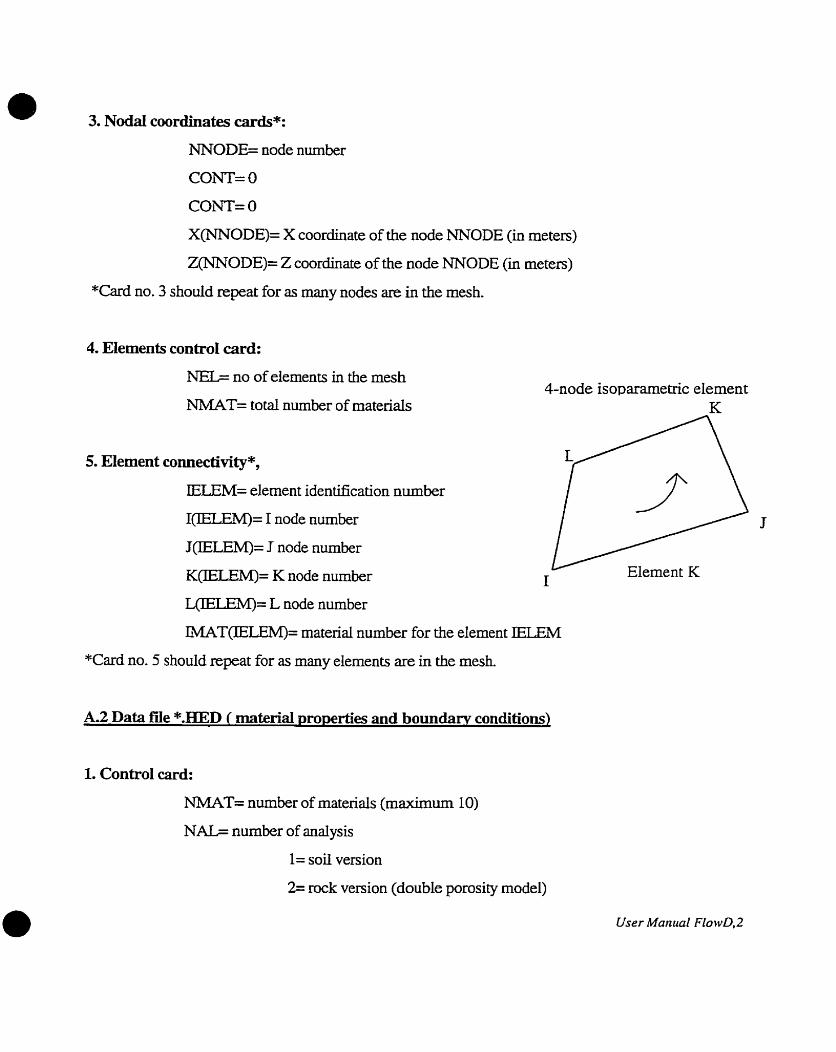
3. Nodal coordinates car&*:

NNODE= node number

corn= O

corn= O

X(NNODE)= X coordinate of the node NNODE (in meters)

Z(NNODE)= Z coordinate of the node NNODE (in meters)

*Card no. 3 shouid repeat for as many nodes are in the mesh.

4. EIements control card:

NEL= no of elements in the mesh

NMAT= total number of materials 4-node isoparametric element

K

5. Elernent connectivity*,

IELEM= elernent identification number

Io= 1 node number J

J(IEI.LEM')= J node nurnber

K O = K node number I Element K

L(IELEM)= L node number

MAT(XLF&I)= material number for the element IELEM

*Card no. 5 should repeat for as many elernents are in the mesh.

A.2 Data file *.KED ( materiai ~roperties and boundary conditions)

1. Control card:

NMAT= number of materials (maximum 10)

N A k number of analysis

1= soi1 version

2= rock version (double porosity model)

User Manual FlowD,2

2. Material properties card:

Soil Version: (one card for each materid, see figures in Chapter 5)

MAT= material identification number

PERMX= pemeability in X direction (in d s )

PERMZ= permeability in Z direction (in mk)

ALFA= angle between the principal axes of permeability and the global system of

coordinates (in degrees)

Rock Version: (one card for each material, see figures Chapter 5)

a. Material identification card

MAT= materid identification number

NSET= number of sets of k t u r e s in material (maximum 10) (in mis)

b. Fractures Hydraulic properties (one card for each set, maximum 10)

PERM(X)= permeability dong the sets of ficictures(in mk)

PERM(Z)= permeability transversal to the set of hcture(in d s )

PLE= arbritary dimension of the rock block large enough to statistically

sample the fractures (m)

EI= average aperture of the h c t u r e s in the set (in meters)

XF= average number of fractures sampled in the set

BETA= angle between the direction of fi-actures set, taken fkom sterenets and

projected on the studied section, measured clockwise fkom the Ox ax

of the global system of coordinates (in degrees)

User Manual FloivD,3

a Specifed total head at the nodes ( DViehlet Boundùry Condition)

a.1 Number of nodes with specified total head; initiaiiy a i i the nodes are

free, at least one node has to have a specifïed total head that has to be

different h m O; as an exarnple; if a slope is satunted, the nodes at the

slope face have total heads equal to the Z coordinate of each paaicular

node (p/y = 0)

=AD= number of nodes with specified head

a.2 Specitied head (for each node one card)

IHEAD= node idenacation where the total head is specified

H E A B total head in node IHEAD (in)

Total head = Z(iHEAD)+pressure head

b. Point source or point sink (Necrmann Boundary condition)

b.1 Number of nodes with specified flow rate

NQNODE= number of nodes with speciiîed flow rate

b.2 SpecEed flow rate

IQNODE= node number point sink or source

QNODE= positive or negative flux magnitude at the node (in m3/s)

+ positive when flow exits the domain

6 negative when flow recharges the domain

c. Disbi6utedflow rate over the side of an element

c.1 Nuniber of elements that have edges with specified distributed head

NQED= number of elements with edges that have specified head

c.2 Specined distributed flow over the edge

NQELEM= element number

MNODEq= edge node number ( as exarnple: node i)

User Manual FlowQ4

NNODEq= edge node number ( as an example: node j)

QDISTR= distributed flow rate over the edge ( in m3/s/meter)

+ positive = enters into the element

+ negative = exits f?om the element

d Drain, weU, and dnrutage gaUery simu&n

Drain: - drain position (node number)

- total head dong the drain = elevation head ( in meters)

Well: - weIl position (node number)

- total head at the botton of the weli = elevation head ( in meters)

- distributed or point source at the bottom of the weii

Druinage gallery: - location of the gallery (node number)

- total head = eievation head ( in meters)

- point source

B. Output file (*.OUT)

1. Header

2. Node nurnber and the total head at that node (one iine for each node)

3. Element number and the directional gradients, total gradient, directional flow velocity, total

flow velocity vector, and its orientation angle at the center of the element (one card for each

element).

User Manual FlowD.5

a Amendix B : NowD cornputer code listing

developed by Doina Pnscu 1997

Dept. of Mining and Metallurgical Engineering McGilI University

THIS PROGRAM PERFORMS FLOW ANALYSE OF 2-DIMENSIONAL PROBLEMS USING 4-NODE ISOPAFSMETRIC ELEMENTS & STEADY STATE CONDITIONS OF FLOW IN HOMOGENEOUS. ISOTROPIC OR ANISOTROPIC DOMAINS,USING SINGLE OR DOUBLE POROSITY MODEL FOR FLOW THROUGH FRACTURED ROCKS.

X(2000),Y(1000)= COORDINATES OF THE NODES XCG( 1000),YCG(lOOû) = COORDINATES OF THE ELEMENT CENTER ID(1000)= ID ARRAY OF THE DOF FOR ALL THE NODES JD(1000)= JD ARRAY OF THE DOF FOR PLL THE NODES N N O D E S = W E R OF NODES NEQ= NUMBER OF EQUATION HD= EWDRAULXC HEAD VECTOR TH= THICKNESS OF THE DOMAiN (=UNITY) N'MAT= NUMBER OF MATERIALS MAT= IDENTIFICATION OF MATERIAL

GRAD( 1000)= GRADIENT MATRIX VELO( t 000)= VELOCITY MATRIX FL( 1000)= LOAD VECTOR PERMX(lO,l)= PERMEABiLITY IN ïlE X DIRECTION PERMY(10,1)= PEl3MEABILlTY IN TKE Y DIRECTION ALFA(10,1)= ANGLE BEïWEEN THE SYSTEM OF COORDINATES AND THE PRINCIPAL

DIRECTIONS OF PERMEABILITY (SOIL VERSION ) PERX(10,l O)=MAJOR PERMEABILITY OF A SET OF FRACTURE PERY(lO,lO)=MINOR PERMEABILITY OF A SET OF FRACTURE PLE(LO,lO)= ARBITRARY DIMENSION OF THE SIDE OF THE BLOCK OF FRACTURED

MEDIUM, LARGE ENOUGH TO STATISTlCALLY SAMPLE THE FAMILIES OF FRACTURES

XF(10, IO)= AVERAGE NUMBER OF FRACTURES IN THE SET EI( 10, IO)= AVERAGE APERTURE OF THE FRACTURES IN THE SET BETA(10, IO)= ANGLE BETWEEN FRACTURES' PREDOMINANT PERMEABILITY &

GOBLAL SYSTEM OF COORDINATES

Program FIorvD (1997) &y D-Priscrr, 1

C N A I , NUMBER OF ANALYSIS = 1 S O L MEDIUM

a C = 2 FRACrURED ROCK MEDIUM C

C IMPLICIT REA4L*4(A-H,O-2) DIMENSION X(lOû0),Y(l000),IC0(4,1000),CON(2,2),L.J(4),~(1000) DIMENSION BF(2,4),TH(1),HEADF(40000),1MAT(1000),ID(1000) DIMENSION CF(4,4),CFG(40000),GRAD( 1 OOO),VELO( 1 OOO),JD( 1 000) DIMENSION FL(40000),VELOS(l),DIRVELO(I),FLE(4),PERMX( 10,l) DIMENSION PLE(IO,10),EI(lO,I O),NSET( IO),PERMY(I O, l),ALFA( IÛ, 1) DIMENSION PERX(lO,lO),PERY(10, IO),MAT(lO),XF(IO, 1 O),BETA(10, 10) DIMENSION XCG( 100O),YCG(1000)

C CHAMCTER TITLE*72 CHARACTER*20 FlLENAME CHARACTEFt*24 CORFILE CHARACTER*24 HEADFILE CHARACTER*24 OUTFILE

C WRITE(*,*) 'INPUT FILE NAME WlTHOUT EXTENSION (MAX 8 CHAEWCTERS):' READ(*,") FILLJAME

C DO 1 ITA=LEN(FEENAME), 1 ,- 1 IF(FILENAME(ITA:ITA).NE.' ') GOTO 2

1 CONTINUE 2 CORFILE=FILENAME(I :ITA)/f COR'

HEADrnE=FrLENAME( 1 :ITA)/f .HED' OuTFILE=FILENAME( 1 :ITA)/f .OUT

C WRITE(*,*) 'OPEN FILES' OPEN (UNIT=20, FILE== ORFILE, STATUS='UNKNOWN',

$ ACCESS='SEQUENTIAL', FORM='FORMATTED') C

OPEN (UNIT=30, FTLE=HEADFILE, STATWS='UNKNOWNf, $ ACCESS='SEQUENTIAL', FORM='FORMATIED')

C OPEN (UNIT=50, F?LE=OUTFILE, STATLTS='UNKNOWN',

$ ACCESS='SEQUENTLAL', FORM='FORMA?TED') C

WRITE(*,*) 'READING THE DATA FILES *.COR & *.HED' READ(20, *) TITLE WRITE(SO,*) 'T'n'LE

C READ(20,*) NNODES

C WRITE(*,*) 'READ THE NODES' DO 10 I= 1 'NNODES

READ(20,*) INODE,DUMY 1 ,DUMY 2,X(I),Y(I) 10 CONTINliE

C WUTE(*,*) 'REAL) TEE ELEMENTS' READ(20, *) NEL,NMAT DO 21 K=l*NEL

Program FlowD (1997) by D. Priscrt, 2

C-- CALCULATE COORDINATES OF THE ELEMENT CENTER------- C

XCG(K)=(X(ICO( 1 ,K))+X(IC0(2,K))+X(IC0(3,K))+X(IC0(4,K)))~4 YCG(K)=(Y(ICO(I ,K))+Y(IC0(2,K))+Y(IC0(3,K))+Y(IC0(4,K)))/4

21 CONTFNUE C

DO 22 I=L,10 22 NSETO=O

CALL PRESET(PERX, 10,lO) CALL PRESET(PERY, 10,lO) CALL PRESET(PLE, IO, 10) CALL PRESET(EI,lO, 1 O) CALL PRESET(BETA, 10.10) CALL PRESET(XF? IO* 10)

CALL PRESET(PERMX, 10.1) CALL PRESET(PERMY, 10.1) CALL PRESET(ALFA, 10-1)

IV-(*,*) 'READ MATERIAL PROPERTIES' READ(30, *) NMAT, NAL DO 40 LL=l,NMAT.

IF (NALEQ. 1) THEN READ(30,*) IMA, PERMX(LL, l), PERMY(LL, l), ALFA(LL, 1)

ELSE READ(30,*) MAT(LL),NSET(MAT(LL)) NSETM=NSET(MAT(LL)) DO 25 M25=L,NSETM

READ(30,*) PERX(LL,M25),PERY(LL,M25),PLE(LL,M25), $ EI(LL,M25),XF(LL,M25),BETA(LL,M25)

25 CONTINUE E N D F

40 CONTINUE C

NNODEL=4 N I C O d m= 1 NU=NVR*NIco NMAX=NVR*h'NODES NVEL=4

C c e - - COMPUTE NUMBER OF NODES WITH SPECIFIED HEAD---------

& BUILD ID =Y

CALL BOUND(ID,HD)

CALL IDJD(ID,NMAX,JD,NEQ)

DO 60 I= 1 ,NEL CALL ELCON(I,ICO.~O,NEL,NNODEL,W,NLJ,JD,NMAX)

CALL BANDW(W.NNODEL,NVR,NW,LBAND) 60 CONTINUE

C WRITE(*,*)'NUMBER OF NODES, NNODES = ',NNODES WRïIE(*,*)'NUMBER OF ELEMENTS, NEL = ' , E L WRITE(*,*)'NUMBER OF EQUATIONS, NEQ = ',NEQ wRrr"E(*,*)'BANDWIDTH, LB AND = ',LBAND

C LSlZE = NEQ * LBANJ3

C CALL PSET(CFG,LSIZE)

C C C A - - - IMTIALIZE AND COMPUTE LOAD VECTOR------ C FROM BOUNDARY CONDITlONS C

WRITE(*,*) 'COMPUTE THE LOAD VECTOR' CALL PSET(FL, 1000)

C CALL LOAD(X,Y ,JD,FL)

C C-- -DO LOOP TO ASSEMBLY THE GLOBAL CHARACTERISnCS

MATRIX AND LOAD VECTOR

WRITE(*,*) 'ASSEMBLY THE LOAD VECTOR' TH= 1 .O

CALL IPLNCF (INEL,IMAT,x,Y , I C O , B F , T H , C O N , C F , N A A , $Ef ,XF,PERX,PERY ,PERMX,PERMY,ALFA)

c ------ MODIEY LOAD VECTOR - KNOWN HEAD --- C -NEUMANN BOUNDARY CONDITIONS- C

CALL PSET(FLE,4) DO 13 J= 1 ,NNODEL

KI=ICO(J,rNEL) IF (ID(KI).EQ,O) THEN DO 14 K= 1 ,NNODEL

U=ICO(K,INEL) IF (ID(KJ).NE.O) THEN

FLE(J')=FLE(J>-CF(J, K) *HD(W) END IF

14 CONTINUE END IF

13 CONTINUE C

CALL ELCON(INEL,ICO.NTCO,NEL,NNODEL,LJ,NLJ,~,NMAX) C

CALL SETUP2(CFG,FL,CF,FLE,NUt W,LB AND) C 200 CONTINLTE

C C - - - SOL= SYSTEM WITH CHOLESKY TECHNIQUE-----------

Program FlowD (1997) by D. Priscu, 4

C WRITE(*,*) 'SOLVE SYSTEM OF EQUATIONS' LLT= 1 CALL CHLS KI(CFG,FL,NEQ,LB AND,LLT,WDETJ)

C c - - - - - P m HEAD AT NODES-- - - - - - - - - - - - C

DO 300 IB=l,NNODES IF(ID(IB).EQ. 1) THEN HEADF(IB)=HD(rB)

ELSE K=ID(IB) HEADF(Il3 )=FL(K)

ENDIF C C

WRITE(50,2030) IB ,HEADF(IB) 2030 FORMAT(/,'AT NODE1,14,11 X,'HEAD=',F 10.4) 300 CONTINUE C c--- CALCULATE GRADIENTS & SEEPAGE VELOCITIES------- C

WRITE(*,*) 'CALCULATE GRADIENTS & SEEPAGE VELOCITIES' WRITE(50,3000)

3000 FORMAT(/, 1X,'ELEMENT,3X,XCG',5X,'YCG1,7X,'GRADX',7X~'GRADY, $5X,'GRADIEW,6X;'VELOX',7X,'VELOY',4Xt'VELOCITYw,5X,'ANGLE')

C C -PREPARE OUTPUT -- C

WUTE(*,*) 'PREPARE OUTPUT DO 400 K= 1 ,NEL

CALL GRADE(K,IMAT,PERMX,PERMY,ALFA,ICO,PERX,PERY, $PLE,EI,BETA,NSET,XF,CON,GRAD,VEiLO,VELOS,GRADOS ,DIRVELO,HEADF,NAL) ~(50,4OOO)ECXCG(K),YCG(K),GRAD(l),GRAD(2),GRADOS,VELO( I), SVEL0(2),VELOS,DIRVELO

4000 FORUT(/,2X,I4,1X,F7.2,1X,F7.2,6(3X,F9.5),3X,F7.2) 400 CONTLNUE C

CLOSE (UNT=20, STATLTS='KEEP') CLOSE (UNIT=30, STATUS='EEP') CLOSE (UNIT=50, STATUS='KEEP')

C STOP END

C C

C ROUTZNE TO COMPUTE THE SPECIFIED VALUES OF THE FIELD VARIABLES C (HYDRAULIC HEAD)

Program FlorvD (1 997) by D.Priscu, 5

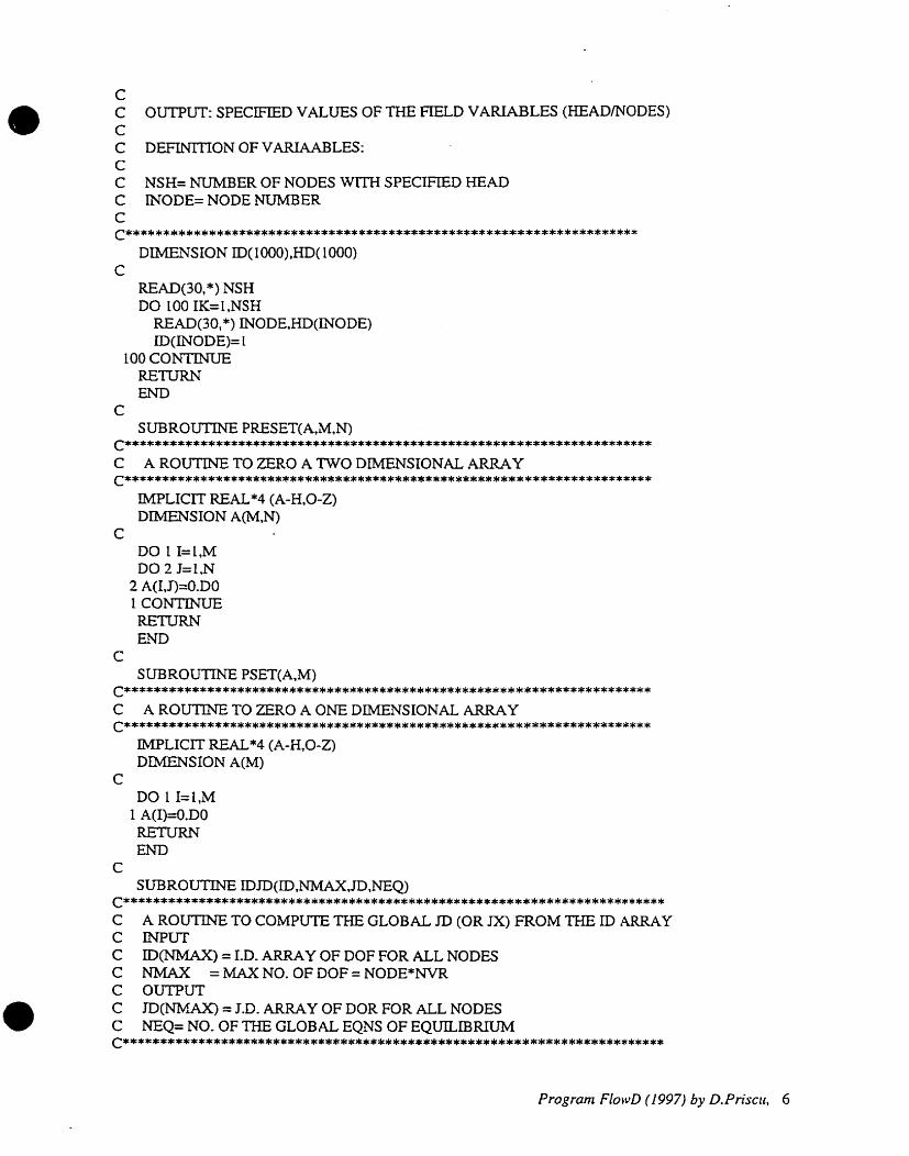
C C OUTPUT: SPECEED VAL,UES OF THE FIELD VARIABLES (HEADINODES) C C DEFINITION OF VARIAABLES: C C NSH= NUMBER OF NODES WJTH SPECIFIED HEAD C INODE= NODE NUMBER

DIMENSION ID( I 000) ,HD( 1000) C

READ(30, *) NSH DO 100 IK=l,NSH

READ(30,*) INODE,HD(INODE) ID(INODE)= 1

100 c o m RETURN END

C SUBROUTINE PRESET(A,M,N)

C********************************************************************** C A ROUTINE TO ZERO A 'LW0 DIMENSIONAL ARRAY C**********************************************************************

IMPLICIT REAL*4 (A-H.0-Z) DIMENSION A(M,N)

C DO 1 I=l,M DO 2 J=l,N

2 A(I,J)=û.DO 1 CONTINUE RETURN END

C SUBROUTZNE PSET(A,M)

c********************************************************************** C A ROIJïlNE TO ZERO A ONE DIMENSIONAL ARRAY C**********************************************************************

IMPLICIT =*4 (A-H,O-2) DIMENSION A(M)

C DO 1 I=1,M

1 A(I)=û.DO RETURN END

C SUBROUTINE IDJD(ID,NMAX.JD,NEQ)

Cf*********************************************************************** C A ROUTINE TO COMPUTE THE GLOBAL JD (OR JX) FROM THE ID ARRAY C INPUT C ID(NMAX) = I.D. ARRAY OF DOF FOR ALL NODES C NMAX = MAX NO. OF DOF = NODE*NVR C OUTPUT C J D o = J.D. ARRAY OF DOR FOR ALL NODES C NEQ= NO. OF THE GLOBAL EQNS OF EQUILISRnrPvi C****t********************************************************************

IMPLICIT REAL*4(A-H.0-Z) DIMENSION ID( 1 OOO), JD( 1 000)

1 CONTINUE EuzruRN E r n

C SUBROUTINE ELCON(IMEL,ICO,MCO,NEL,NNODEL.LJ,NLJ,JX,NMAX)

........................................................................... C C A ROUTINE TO BUILD ELEMENT CONNECTIVITY ARRAY W. THE ROUTINE IS C CALLED IN A LOOP OVER ALL ELEMENTS. C INPUT: C IE =ELEMENT NO, IN THE DO LOOP C ICO(NIC0,NEL) =GLOBAL CONNECTIVITY MATRIX C M C 0 =NO. OF ROWS OF CONNECTIVrrY MATRLX C NEL =TOTAL NO. OF ELEMENTS C N V R =NO. OF VARIABLES (DOF) PER NODE C NNODEL =NO. OF NODES PER ELEMENT C JX(NMAX) =GLOBAL ID AREUY C NMAX =MAX NO. OF DOF= NODES*NVR C OUTPUT: C UWJ) =ELEMENT CONNECTIVITY ARRAY C c********************************************************************

ZMPLICIT REAL*4 (A-H,O-Z) DIMENSION W ( N L J ) , I X ~ , I C O ( M C O , N E L )

C DO 2 J= 1,NNODEL

J2=(IC0(ITINEL)) ljg')=jx(j2)

2 CONTINUE R E m END

C SUBROUTINE LOAD (X,Y,JD,FLUX) IMPLICIT REAL*4 (A-H,O-Z)

c******************************************************************** C C A ROUTINE TO COMPUTE LOAD VECTOR OVER THE BOUNDARY OF THE C DOMAIN-NEUMANN BAUNDARY CONDITIONS. C C INPUT: C FLUX(INODE)= SPECIFlED FLOW RATE IN NODES C QFLUX= VALUES OF THE FLUX OVER TEE BOUNDARY (DISTRIBUTED LOAD) C OUTPUT: C NODE . - FLUX IN THE NODE C LOADVECTOR C

c******************************************************************** DIMENSION FLUX( looo),m( iooo>,~r ; tvx( r OO),QNODE( 100) DIMENSION X(l),Y(l)

C C------ COMPUTE NODE WITH SPECIFIED FLOW RATE ---

-NEUMANN BOUNDARY CONDITION--

READ(30,*) NQNODE

175 CONTINUE C C-- COMPUTE UNIT FLUX OVER TEE SIDE OF AN ELEMENT----- C --NEUMANN BOUNDARY CONDITION-- C

READ(30,*) NQSIDE C

DO 185 N=l,NQSIDE READ(30,*) IELE,NODEI,NODE.J,QFLUX(IELE) LLJ=((X(NODEI)-X(NODl3))**2+(Y(NODEI)-Y(NODEJ))**2)**( 1/21 QSIDEI=(QFLUX(IELE) *Lm12 QSIDEJ=(QFLUX(IELE)*LU)/2 KI=JD(NODEI) KJ=.lD(NODEJ) FLUX(KI)=FLUX(KI)+QSTDEI ETUX(KJ)=FLUX(KJ)+QSIDEJ

185 CONTINUE RET'URN END

C SUBROUTLNE IPLNM\I(S,T,SF,DSFS,DSFr)

C*****************X*************************************************

A ROUTINE TO COMPUTE THE SHAPE FUNCTIONS AND THEIR DERIVATES AT A POINT (S,T) WITHIN THE 4-NODE ISOPARAMETRIC ELEMENT. INPUT DATA: S = NONDIMENSIONAL S-COORDINATE OF THE POINT T = NONDIMENSIONAL T-COORDINARE OF THE POINT IN = INDEX FOR CALCULATEJSKIP THE SHAPE ECMCTION SF(4) OUTPUT SF = SHAPE FUNCIIONS (4) DSFS= (DNIDS) DSFT= (DN/DT)

IMPLICIT REAL*4 (A-H,O-2) DIMENSION SF(4),DSFS(4),DSFT(4)

C SF(l)= l./4.*(l.+S)*(l .+T) SF(2)=1./4.*(1.-S)*(I.+T) SF(3)=1./4*(1.-S)*(i .-T)

SF(4)=1./4.*(1 .+S)*(l .-T) C

DSFS(l)= 1 ./4.*(l.+T) DSFS(2)=- 1 J4.*(l .tT) DSFS(3)z- lJ4.*(l .-T) DSFS(4)= 1 J4.*(l .-T) DSFT(1)=1 J4.*(l .+S) DSFmT(2)= 1 ./4.*(1 .-S) DSFT(3)=- 1 J4.*( 1 .-S) DSFT(4)z- 1J4.*( l.+S) RETURN END

C SUBROUTINE PLNBJ (SF,DSFS,DSR,X,Y,M,AI,WDETJ,BF,S,T) IMPLICIT REAL*4 (A-H,O-Z)

c******************************************************************** C C A ROUTINE TO COMPUTE THE STRAIND-DESPLACEMENTS MATRlX BF(2,4) AT C A POINT (X,Y) wlTHlN THE 4-NODE ISOPARAMETRJC ELEMENT C C SF = SHAPE FUNCTION C DSFS & DSFT DERIVATES OF TEE SHAPE FUNCTIONS C AJ = JACOBIAN MATEUX C WDETJ = DETERMINANT OF THE JACOBIAN MATRUC C AI = INVERSE OF JACOBIAN MATRlX C*****************************************************************

DIMENSION SF(4),DSFS(4),DS~(4),X(4),Y(4),BF(2,4),AJ(2,2),M(2,2) DIMENSION S(4),T(4)

C CALL PRESET(AI,2,2)

C CALL IPLNNN(S,T,SF,DSFS,DSFT) CALL PRESET(AJ,2,2)

C DO I K=1,4

AJ(1,I )=AT( l,l)+DSFS(K)*X(K) AJ( I ,2)=AJ(1,2)+DSFS(K)*Y(K) AJ(2,l )=AJ(Z,l)+DSFT(K) *X(K) AJ(2,2)=AJ(2,2)+DSFT(K) *Y (K)

1 CONTINUE C

WDETJ=AJ(I, l)*AJ(2,2)-A.J(l12)*AJ(2, 1) CDUM l=AJ(l, 1)/WDETJ AI(l,I)=AJ(2,2)/WDETJ AI( 1,2)=-AJ(1 ,S)/WDETJ AI(2,1)=-AJ(2,l)/WDETJ AI(2,2)=CDUM 1

C DOSJ=1,4 BF(1 ,J)=AI(1,1)*DSFS(J)+A1(1,2)*DSFT(J) BF(~,~)=AI(~,~)*DSFS(J)T)~AI(~,~)*DSFT(J)

5 CONTINUE m. dRN END

C

C SUB ROUTINE IPLNCF(I,IMAT,X,Y ,ICO,B F,TH,CON,CF,NAL,NSET,PLE,B ETA, $EI,XF,PERX,PERY,PERMX,PERMY,ALFA) TMPLICIT REAL*4 (A-H,O-Z)

c*****************************f**f************************************ A ROUTINE TO COMPUTE THE ELEMENT CHARACTERISTICS MATRIX

INPUT: XX,YY=ELEMENT NODAL X,Y COORDINATES (EACH 4) X,Y= NODAL X,Y COORDINATES TH= ELEMENT THICKNESS CON(2,2)= ELEMENT CONDUCTIVITY MATRIX BF(2,8)= B MATRI[X

OUTPUT: CF(4,4)= ELEMENT CHARACTEEUSTICS MATRIX

DIMENSION XX(4),YY(4),X( 1000),Y( 100O),CF(4,4),BF(2,4),SF(4) DIMENSION DSFS(4),DSFT(4),W(2),IC0(4,lOOO),CON(2,2),PLE(10,10) DIMENSION VSI(4),VTI(4),WE(4,4),AK(4,4),iMAT( 1 ),NSET( IO) DIMENSION ALFA(1O11),PERMX(10, 1 ),PERMY(10, I),PERX( 1 O, 10) DIMENSION PERY( 10,lO) DIMENSION XF(lO,lO),BETA( IO, lO),EI(lO, 10)

C W(l)=l.O W(2)=W( 1)

C CALL PRESET(CFA,4)

C C---- COMPUTE HYDRAULIC CONDUCTIVITY MATFUX--------

FOR DmRENT TYPES OF ANALYSE NAL=l SOIL VERSION NAL=2 DOUBLE POROSITY VERSION

IF (NALEQ. I ) THEN CALL CARASO(I,IMAT,PERMX,PERMY ,ALFA,CON)

ELSE

CALL DPOR(I,IMAT,PLE,EI,CON,BETA,NSET,XF,PERX,PERY> ENDIF

DO 25 LL= 1 ,4 LNODE=ICO(LL,I) XX(LL)=X(LNODE) YY(LL)=Y (LNODE)

25 CONTINUE C C- COORDINATES OF THE GAUSS INTEGRATION POINTS C

VSI(l)=- f /SQRT(3.0) vn( l)=VSI( 1 ) vs I(2)=VSI( 1) vn(2)=-VSI( 1 ) VSI(3)=-VSI( 1)

C

CALL IPLNBJ(SF,DSFS.DSFT,XX,YY.AJ,AI,WDETJ,BF.SI.n) TH= 1 .O CAST=WDETJ*TH CALL TRANS(CON,BF,AK,WE,2,4,CASJ? DO 35 NL=1,4 DO 15 -1.4 CF(NL,ML)=CF(NL,ML)+AK(NLTML)

15 CONTINUE 35 CONTINUE 1 IO CONTINUE do 1 I l l j=l,4 do 1121 m=1,4

1121 continue I l 1 1 continue

RETtlRN END

C SUBROUTINE GRADE(I,IMAT,PERMX,PERMY,ALFATICOtPERX,PERY, $PLE,EI,BETA,NSET,XF,CON,GRAD,VELO,VELOS ,GRADOS ,DIRVELO,HEADF,NAL)

C IMPLLCIT REAL*4 (A-H.0-2)

C******************************************************************** C C A ROUTINE TO COMPUTE GRADIENTS & VELOCITTES AT CENTRE OF THE C ELEMENT IN X & Y DIRECTION. C C INPUT: C HD(lNODE)=VALUES OF TWE HYDRAULIC HEAD IN NODE INODE C BF(2,4)= MATRIX C SC & TC= LOCAL COORDONATES OF THE CENTER OF TKE ELEMENT C C OUTPUT: C GRADX & GRADY= GRADIENTS IN X & Y DIRECTION. C c********************************************************************

DIMENSION GRAD(2),VEL0(2),ICO(4,I),HEADF(lOOO),BF(2,4),CON(2,2) DIMENSION PERMX(lO,l),PERMY(lO, l),ALFA(lO, l),VELOS(l),GRADOS(l) DIMENSION DIRVELO(l),PLE(lO, lO),PERX(lO, 10),PERY(10,10) DIMENSION EI(10,10),XF(10,10),BETA(IO, 1)

C c------ COMPUTE GRADLENTS AT THE CENTER OF THE ELEMENT------ C

CALL PSET(GRAD,2) scs.0 TC=O.O

Program Flo wD (1 997) by D. Priscrr, 1 1

CALL IPLNB J(SF,DSFS,DSFT.X,Y ,N,AI, WDETJ,BF,SC,TC) DO 55 K= 1-2

DO 65 L= 1.4 GRAD(K)=GRAD(K)+(BF(K,L)*HEADF(ICO(L,l)))

C 65 C O m c 55 c o r n

C IF (NALEQ. 1) THEN CALL CARASO(I,IMAT,PERMX,PEWY,ALFA,CON)

ELSE C U L DPOR(I,IMAT,PLE,EI,CON,BETA,NSET,XF,PERX,PERY)

ENDIF CALL PSET(VEL0,2)

C DO 70 L=1,2

DO 75 K=1,2 VELO(L)=VELO(L)-(CON(L,K)*GRAD(K))

75 CONTINUE 70 CONTINUE

C GRADOS=((GRAD(1))**2+(GRAD(2))**2)**(0.5) VELOS=((VELO( 1))**2+(VEL0(2))**2)**(0.5) DIRVELO=(ATAN2(VELO(2),VELO(l)))* l80/3.141593 RETURN END

C SUBROUTINE TRANS(S,T,R,W,M 1 ,M2,CONST) MPLICIT REAL*4 (A-H,O-2)

C THIS ROUTINE MULTIPLIES 3 MATRICES IN THE FORM: C (R) = CONSTANT * (T)TRANSPOSE * (S) * (T) c********************************************************************

DIMENSION S(M I ,M l),T(M l,M2),W(M2,M l),R(M2,M2) C

CALL PRESET(R,M2,M2) CALL PRESET(W,M2,M 1) DO 10 I=I,M2 DO 10 J=l,MI DO 10 K=l,Ml

1 O W(I,J)=Wfl,J)+CONST*T(K,I)"S(K,J) DO 20 I=l,M2 DO 20 J= 1 ,M2 DO 20 K=1,M1

20 R(I,J)=R(I,J)+W(I,K)*T(Kn R E r n END

C SUBROUTDE B.4NDWH(LI,NNODEL,NVR,NW,LBAND) IMPLICIT REAL"4 (A-H,O-2)

c********************************************************************* C THTS ROUTINE CALCULATES HALF BAND WIDTH OF THE GLOBAL STIFFNESS C MATRUC:. THE ROUTINE SHOULD BE CALLED IN A LOOP FOR ALL ELEMENTS. C INPUT C LJ(NLJ)= ELEMENT DOF OR CONNEC- ARRAY

Program FlowD (1997) by D.Priscrc. 12

C NNODEL= NO. OF NODES PER ELEMENT C NVR= NO. OF VARIABLES(D0F) PER NODE C NLJ=NVR*NNODEL C OUTPUT C LBAND= MATRIX HALF BANDWIDTH INCLUDING THE DIAGONAL C*********************************************************************

DIMENSION LJ(NLJ) C

MAX* MIN= 1 0000 NV=NVR*NNODEL DO 10 J=l,NV

IF(LJ(J).EQ.O) GO TO 10 IF(LJ(J).GT.MAX)MAX=U(J) rl=(W(J).LT.MIN)MIN=LI(J)

10 CONTJNUE NB=MAX-MIN+ 1 IF(NB .GT.LBAND) LB AND=NB R E r n END

C C

SUBROUTINE CHLSKi;(A,B,NEQ,LBAND,LLT,WDETJ) IMPLICIT REAL*4 (A-H,O-2)

c********************************************************************* C THIS ROUTINE SOLVES THE EQUATION : P= (K).(DELTA) , FOR THE DIS- C PLACEMENT VECTOR (DELTA), BY MEANS OF CHOLESIU DECOMPOSITION C INPUT C A =GLOBAL MATRIX IN BANDED FORM C B =GLOBAL LOAD VECTOR C NEQ =NO. OF EQUATIONS C LBAND =HALF BANDWIDTH OF GLABAL STIFFNESS MATRIX C LT =INDEX, = 1 FOR FORWARD ELIMINTATION AND BACKSUBSTITUTION C =ANY OTHER VALUE FOR SUBSTITUTION ONLY C NMAT STORAGE SIZE OF GLOBAL STIFFNESS MATRI[X = NEQ*LBAND C OUTPUT C B =DISPLACEMENT VECTOR c*****************************************************************

DIMENSION A(1 ),B(neq) LLT=1 WDETJ=O.O MM=LBAND- 1 NM=NEQ*LB AND NM I=NM-MM IF (LLT.NE. 1) GO TO 55 MP=LBAND-i- 1 KK=2 FAC=WDETJ A(I)=l JSQRT(A(1)) BIGL=A( 1 ) S f i A ( 1 ) A(2)=A(2)*A(l) A(MP)= I JSQRT(A(MP)-A(S)*A(2)) IF(A(MP) .GT.B IGL)B IGL=A(MP) IF(A(MP).LT.SML)SML=A(MP)

MP=MP+LB AND DO 62 J=MP,NM 1 ,LB AND JP=J-MM M z C d IF(KK.GE.LBAND) GO TO 1 KK=KK+l II= 1 IC= 1 GO TO 2

1 KK=KK+LBAND II=KK-MM JC=KK-MM

2 DO 65 I=KK,JT,."VIM IF(A(I).EQ.O.)GO TO 64 GO TO 66

64 JC=JC+LBAND 65 MZC=MZC+l

ASUMl=û. GO TO 61

66 MMZC=MM*MZC Ir=IItMZC KM=KK+MMZC A(KM)=A(KM)*A(JC) IF(KM.GE.P)GO TO 6 KïI=KM+MM DO 5 I=KJ,P,MM - ASUM2=û. IM=I-MM II=IIt 1 KI=II+MMZC DO 7 K=KM,IM,MM ASuMz=ASUM2+A(ra)*A(K)

7 KI=KI+MM 5 A(&(A(I)-ASUM2)*A(E(I) 6 CONTINUE

ASUMl=û. DO 4 K=KM,P,MM

4 ASUM l=ASUM l+A(K)*A(K) 6 1 S=A(J)-ASUM I

IF(S .LT.O.)WDETJ=S IF(S .EQ.O.)WDETJ=O. IF(S.GT.O.)GO TO 63 NRO W=(f+MM)/LB AND WRITE(6,99) NFtOW

99 FORMAT(35H ERROR CONDITION ENCOUNTERED IN ROWJ6) RETmw

63 A(J)= I JSQRT(S) IF(A(J).GT.B 1GL)B IGL=A(J) IF(A(J).LT.SML)SML=A(J)

62 CONTINUE IF(SML.tE.FAC*BIGL)GO TO 54 GO TO 53

54 WBETJ=O. RETURN

53 WDETJ=SMUBIGL

Program FloivD (1997) by D. Priscrr, 14

55 B(l)=B(l)*A(l) KK= 1 KI= 1 .J= 1 DO 8 L=2,NEQ BSUM l=O. LM=L- 1 J=J+LB AND IF(KK.GE.LBAND)GO TO 12 KK=KK+ I GO TO 13

12 KK=KK+LB AND Kl=Kl+l

13 JK=KK DO 9 K=Kl,LM BSUMl=BSUMi+A(JK>*B(K) JK=JK+MM

9 CONTINUE 8 B(L)=(B(L)-BSUMl )*A(J)

B(NEQ)=B@EQ)*A@JM 1) NMM=NM 1 NN=NEQ- 1 ND=NEQ DO 10 G-1,NN BSUM2=O. NLFNEQ-L NL I =NEQ-L+ 1 NMM=NMM-LBAND NJ1=NMM IF(TiGE.LBAND)ND=ND- L DO 11 K=NLl,ND NJ l=NJ 1 + 1 BSUM2=BSUML+A(NJl)*B(K)

I l CONTINUE i O B(NL)=(B(NL)-BSUM2)*A(NMM)

RETURN END

C SUBROUTINE SETUP2(A,BB,S,m,NU;UVLBAND) IMPLICIT REAL*4 (A-H,O-Z) c**************************************************************************

C A ROUTINE TO ASSEMBLE THE GLOBALAL STIFFNESS MATRIX USING A UNIFORM C BAND WIDTH LBAND. IT ALSO ASSEMBLES THE GLOBAL LOAD VECTOR. THIS C ROUTINE SWOULD BE CALLED IN A LOOP OVER ALL ELEMENTS. C INPUT C INEL =ELEMENT NUMBER IN DO-LOOP C S(NLJ,NW) =ELEMENT STïFJ3ESS MATRM C F L O =ELEMENT LOAD VECTOR C NLJ =NO. OF DOF PER ELEMENT C L J o =ELEMENT CONNECTIVITY ARRAY C LBAND =HALF BANDWIDTH C OUTPUT C A =GLOBAL STIFF'NESS MATRlX IN BANDED FORM C B =GLOBAL LOAD VECTOR c***********************************************************************

i O K=(LJC- 1)*LB + UR GO TO 13

9 K=(L.R-L)*LB + LJC 13 A(K)=A(K)+S(I,J) 11 CONTINUE 12 CONTINUE

RETURN END

C SUBROUTINE CARASO(I.IMAT,PERMX,PERMY,AL.FA,CON) IMPLICIT REAL*4(A-H,O-2)

C******************************************************************** C A ROUTINE TO COMPUTE THE CHARATERISTICS MATRIX FOR THE SINGLE C POROSITYCASE C C INPUT: C I= ELEMENT NUMBER C PERMX= PERMEABEITY X DIRECIION C PERMY= PERMEABILY IN Y DIRECTION C ALFA= ANGLE BETWEEN THE GLOBAL. SYSTEM OF COORDINATES & C DIRECTIONAL PERMEABILITIES C CON(2,2)= CHARACTERISTICS MATRIX C C***********+********************************************************

DIMENSION PERMX(l0,l ),PERMY(lO, 1),ALFA(10, l),CON(2,2),IiVIAT(l) MID=IMAT(I) ALFAR=(ALFA(MID, l)*3.l4 l593)f 180 CALL PRESET(CON, 2,2)

CON(1,l) = PERMX(MID, I)*(COS(ALFAR))**2 + $ PERMY(MID, l)*(SIN(ALFAR))**2

CON(2,2) = PERMX(MD, f)*(SIN(ALFAR))*"2 +- $ PERMY(MID, 1) *(COS(ALFAR))**2

CON( 1,2) = PERMX(MTD, l)*(SIN(ALFAR)) *(COS(ALFAR))- $ P E R M Y o , 1 )*(SIN(ALFAR))*(COS(ALFAR))

CON(2,l) = CON( 1,2) RETllRN END

SUBROUTINE DPOR(I,IMAT,PLE,EI,COND,BETA,NSET,XF,PERX,PERY) IMPLICIT REAL*4 (A-H,O-2)

C******************************************************************** C A ROUTINE TO CALCULATE THE ELEMENT CONDUCTIVITY MATRM C IN THE DOUBLE POROSITY APPROACH, TAWNG IN ACCOUNT C ORIENTATION OF THE FRACTURES AND =IR HYDRAULIC PROPERTIES

C C INPUT: C C

DIMENSION COND(2,2),PLE(10,1O),EI(lO, lO),PERX(lO, lohPERY(10~ 10) DIMENSION CONI(2,2) DIMENSION NSET(lO),IMAT(I ),XF(lO,lO),BETA( lO,10)

C C- COMPUTE DIRECTIONAL M A T R f X - - - - - - C

CALL PRESET(COM,2,2) CALL PRESET(COND,2,2) KMID=IMAT(I) DO 1 000 II= 1 ,NSET(KMTD) BETAR=(BETA(KMlD,rr)*3.14 I593)/l8O CONI(l,l)= PERX(KMID,II) * (COS(E3 =AR))* *2 + $ PERY (KMID,II) * (SIN(B ETAR)) * *2 CONI(212)= PERX(KMLDyII) * (SIN(BETAR))* *2 +

$ PERY(KMIDJI) * (COS(BETAR))**2 CONT(l,2)=(PERX(~,n>-PERY(KMID,rr))* $ (SIN@ ETAR)) *(COS (B ETAR)) CONI(2,1)=CONI(1,2)

C DO 1200 KK=1,2

DO I300JJ=1,2 - COND(KK,JJ)=cOND(KK*JJ)+( IIPLE(KMID,II))*(EI(KMID,rI))*

s P(KMID~~)*(CONCKK,J~) 1300 C0NTrNU-E 1200 CONTINUE 1000 CONTINUE C

RETURN END

IMAGE NALUATION TEST TARGET (QA-3)

APPUED IMAGE. lnc - - - 1653 East Main Street - -. - - Rochester, NY 14609 USA -- -- - A Phone: 71 6/482-0300 -- -- - - Fa: 71 6/288-5989

Q 1993. Applied Image. Inc.. Al1 Rights Resewed