Double Clamped and Cantilever Beam Theoretical Solution and

Numerical Solution by Finite Element Method

Anastasios S. Lazaridis

M. Eng. in Electrical Engineering & Computer Science

tasoslazaridis13@gmail.com

Abstract—This paper presents a static analysis of a beam

made of Aluminum. Two cases are studied, the Double Clamped

Beam and the Cantilever Beam problem. The displacement of the

beam under a load is calculated theoretically using Calculus of

Variations and numerically using Finite Element Method (FEM).

Numerical results are obtained by ANSYS and SOLIDWORKS

software. All results are compared and relative differences are

calculated.

Keywords—static analysis; calculus of variations; FEM;

ANSYS Workbench; beam displacement; SolidWorks;

I. THEORETICAL PROBLEM AND SULUTION

A. Definition of the Problem

Suppose a beam of length l having uniform cross section

under a load. Let 3: 0,y l , describe the shape of the

axis of the beam and 3: 0,l be the load per unit

length on the beam. Assuming small deflections, the potential

energy from elastic forces [2] is the functional 3: 0,eV l

22

2

0 02 2

l l

e

EI d y EIV dx y dx

dx (1)

where E is the modulus of elasticity and I is the moment of inertia, both are constants. The potential energy from

gravitational forces [2] is the functional 3: 0,gV l

0

l

gV ydx (2)

The total potential energy is the functional 3: 0,V l

2

0

, ,2

lEI

V V x y y y y dx

(3)

The shape of the beam is such that V is minimum. The

Lagrangian function 3 0,f l is

2, ,

2

EIf x y y y y (4)

must satisfy the Euler-Lagrange equation [1]. The Euler-Lagrange Equation for a functional involving second-order derivatives is written

2

20

d f d f f

dx y dx y y

(5)

along with the condition

3

0

0 ,

x l

x

f d f f

y dx y y

(6)

The above equation spawns the four boundary conditions

0

0x

f

y

(7)

0

x l

f

y

(8)

0

0

x

d f f

dx y y

(9)

0

x l

d f f

dx y y

(10)

This produces the differential equation

(4) , 0,

xy x x l

EI

(11)

The general solution of the differential equation (11) is the function

3 2+ + , 0,y x h x Ax Bx Cx D x l (12)

where , , ,A B C D are constants and h x is a partial solution of

the differential equation (11), where

(4) =x

h xEI

(13)

B. Definition of the load

In this paper constant load case is studied

, 0,x P x l (14)

So the total impressed force on the beam is

0

l

F x dx Pl (15)

C. Moment of Inertia

The moment of inertia of an area with respect to an axis is the sum of the products obtained by multiplying each element of the area dA by the square of its distance from the axis [3].

For a section in the yx plane, the moment of inertia, about y

and x axis respectively, is defined to be the double integral

2

y

A

I x dxdy (16)

2

x

A

I y dxdy (17)

In the case of rectangular area centered at the origin of yx

plane (Fig. 1), A is the region , ,2 2 2 2

a a b bA

. So yI

and xI are calculated

32

12y

A

a bI x dxdy (18)

32

12x

A

abI y dxdy (19)

Fig. 1. Rectangular area centered at the origin of yx plane.

II. BEAM CAD MODEL

The CAD model of the beam is shown in Fig. 2. The material of the beam is Aluminum Alloy AA380.0-F die. The dimensions of the beam are shown in figure and the material properties are shown in Table I.

Fig. 2. The CAD model of the beam made of Aluminum and the dimensions

of the beam.

TABLE I. MATERIAL PROPERTIES OF THE ALUMINUM BEAM

Material Properties Property Value Unit

Elastic Modulus 71000 N/mm2

Poisson’s Ratio 0.33 N/A

Shear Modulus 26500 N/mm2

Mass Density 2760 kg/m3

Tensile Strength 317 N/mm2

Yield Strength 159 N/mm2

Thermal Conductivity 109 W/(m·K)

Specific Heat 963 J/(kg·K)

III. DOUBLE CLAMPED BEAM

A. Theoretical Solution

Suppose that the beam is clamped at each end (Fig. 3). The beam is “fixed in the wall” at each end so that at 0x and

x l we have respectively 0 0 0y y and 0y l y l .

Fig. 3. The beam is clamped at each end.

Here, there are four imposed boundary conditions. All the allowable variations in this problem require that

0 0 0 and 0l l so that no natural boundary

conditions (6) arise.

So the problem is subscribed by the set of equations below

(4) , 0,

0 0 0

0

Ply x x l

EI

y y

y l y l

(20)

The general solution of the system of equations (20) is the polynomial function

24 3 2+ + , 0,

24 12 24

P Pl Ply x x x x x l

EI EI EI (21)

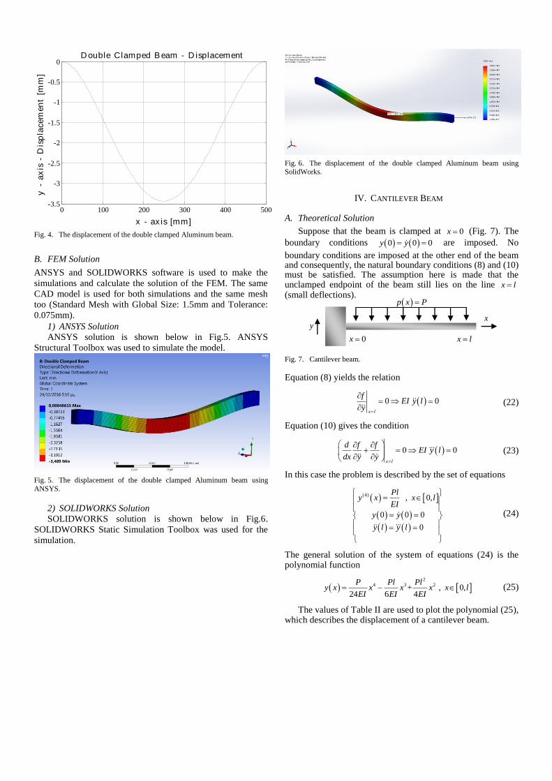
The values of Table II are used to plot the polynomial (21), which describes the displacement of a double clamped beam.

TABLE II. NUMERICAL VALUES OF THE VARIABLES

Variable Values Variable Symbol Value Unit

Elastic Modulus E 71000 N/mm2

Area Moment of Inertia I 6666.67 mm4

Length of Beam L 500 mm

Load per unit Length P 10 N/mm

x

y

0x x l

p x P

x

y

a

b

0 100 200 300 400 500-3.5

-3

-2.5

-2

-1.5

-1

-0.5

0

x - ax is [mm]

y-

ax

is-

Dis

pla

cem

en

t[m

m]

D ouble Clamped B eam - D isplacement

Fig. 4. The displacement of the double clamped Aluminum beam.

B. FEM Solution

ANSYS and SOLIDWORKS software is used to make the

simulations and calculate the solution of the FEM. The same

CAD model is used for both simulations and the same mesh

too (Standard Mesh with Global Size: 1.5mm and Tolerance:

0.075mm).

1) ANSYS Solution

ANSYS solution is shown below in Fig.5. ANSYS

Structural Toolbox was used to simulate the model.

Fig. 5. The displacement of the double clamped Aluminum beam using

ANSYS.

2) SOLIDWORKS Solution

SOLIDWORKS solution is shown below in Fig.6.

SOLIDWORKS Static Simulation Toolbox was used for the

simulation.

Fig. 6. The displacement of the double clamped Aluminum beam using

SolidWorks.

IV. CANTILEVER BEAM

A. Theoretical Solution

Suppose that the beam is clamped at 0x (Fig. 7). The

boundary conditions 0 0 0y y are imposed. No

boundary conditions are imposed at the other end of the beam and consequently, the natural boundary conditions (8) and (10) must be satisfied. The assumption here is made that the unclamped endpoint of the beam still lies on the line x l (small deflections).

Fig. 7. Cantilever beam.

Equation (8) yields the relation

0 0

x l

fEI y l

y

(22)

Equation (10) gives the condition

0 0

x l

d f fEI y l

dx y y

(23)

In this case the problem is described by the set of equations

(4) , 0,

0 0 0

0

Ply x x l

EI

y y

y l y l

(24)

The general solution of the system of equations (24) is the polynomial function

24 3 2+ , 0,

24 6 4

P Pl Ply x x x x x l

EI EI EI (25)

The values of Table II are used to plot the polynomial (25), which describes the displacement of a cantilever beam.

x l 0x

y

p x P

x

0 100 200 300 400 500-180

-160

-140

-120

-100

-80

-60

-40

-20

0

x - ax is [mm]

y-

ax

is-

Dis

pla

cem

en

t[m

m]

Cant i lever B eam - D isplacement

Fig. 8. The displacement of the cantilever Aluminum beam.

B. FEM Solution

ANSYS and SOLIDWORKS software is used to make the

simulations and calculate the solution of the FEM. The same

CAD model is used for both simulations and the same mesh

too (Standard Mesh with Global Size: 1.5mm and Tolerance:

0.075mm).

1) ANSYS Solution

ANSYS solution is shown below in Fig.5. ANSYS

Structural Toolbox was used to simulate the model.

Fig. 9. The displacement of the cantilever Aluminum beam using ANSYS.

2) SOLIDWORKS Solution

SOLIDWORKS solution is shown below in Fig.6.

SOLIDWORKS Static Simulation Toolbox was used for the

simulation.

Fig. 10. The displacement of the cantilever Aluminum beam using

SolidWorks.

V. RESULTS

A. Double Clamped Beam

TABLE III. DOUBLE CLAMPED BEAM – DISPLACEMENT

Displacement of Double Clamped Beam [mm]

Theoretical ANSYS SolidWorks

3.438 3.489 3.489

TABLE IV. DOUBLE CLAMPED BEAM – RELATIVE PERCENT

DIFFERENCES

Relative Percent Differences

ANSYS Theoretical

SolidWorks 0% 1.462%

ANSYS - 1.462%

B. Cantilever Beam

TABLE V. CANTILEVER BEAM - DISPLACEMENT

Displacement of Cantilever Beam [mm]

Theoretical ANSYS SolidWorks

165.05281 164.88011 157.86049

TABLE VI. CANTILEVER BEAM – RELATIVE PERCENT DIFFERENCES

Relative Percent Differences

ANSYS Theoretical

SolidWorks 4.257% 4.357%

ANSYS - 0.104%

REFERENCES

[1] I. M. Gelfand and S.V. Fomin, “The Canonical Form of the Euler equation and related topics,” in Calculus of Variations, (Translated and Edited by Richard A. Silverman), New Jersey: Prentc Hall, 1963.

[2] Bruce van Brant, “Problems with Variable Endpoints,” in The Calculus of Variations, New York: Springer-Verlag, 2004, pp. 140-145.

[3] Walter D. Pilkey, “Geometric Properties of Plane Areas,” in Formulas for Stress, Strain and Structural Matrices, 2nd ed., Ney Jersey:John Wiley & Sons, 2005, pp. 19-21.