DOT/FAA/AR-09/10

Air Traffic Organization Operations Planning Office of Aviation Research and Development Washington, DC 20591

Data and Analysis for the Development of an Engineering Standard for Supercooled Large Drop Conditions March 2009 Final Report This document is available to the U.S. public through the National Technical Information Services (NTIS), Springfield, Virginia 22161.

U.S. Department of Transportation Federal Aviation Administration

NOTICE

This document is disseminated under the sponsorship of the U.S. Department of Transportation in the interest of information exchange. The United States Government assumes no liability for the contents or use thereof. The United States Government does not endorse products or manufacturers. Trade or manufacturer's names appear herein solely because they are considered essential to the objective of this report. This document does not constitute FAA certification policy. Consult your local FAA aircraft certification office as to its use. This report is available at the Federal Aviation Administration William J. Hughes Technical Center's Full-Text Technical Reports page: actlibrary.tc.faa.gov in Adobe Acrobat portable document format (PDF).

Technical Report Documentation Page 1. Report No. DOT/FAA/AR-09/10

2. Government Accession No. 3. Recipient's Catalog No.

5. Report Date

March 2009 4. Title and Subtitle

DATA AND ANALYSIS FOR THE DEVELOPMENT OF AN ENGINEERING STANDARD FOR SUPERCOOLED LARGE DROP CONDITIONS

6. Performing Organization Code

7. Author(s)

Stewart Cober1, Ben Bernstein2, Richard Jeck3, Eugene Hill4, George Isaac1, Jim Riley3, and Anil Shah5

8. Performing Organization Report No.

10. Work Unit No. (TRAIS)

9. Performing Organization Name and Address 1Cloud Physics and Severe Weather Research Section Environment Canada 4905 Dufferin Street Toronto, Ontario M3H5T4 Canada

2Leading Edge Atmospherics, LLC 3711 Yale Way Longmont CO 80503

3Federal Aviation Administration William J. Hughes Technical Center Airport and Aircraft Safety Research and Development Group Flight Safety Team Atlantic City International Airport, NJ 08405 4Eugene G. Hill 5537 26th Avenue S Seattle, WA 98108-3050 5Anil D. Shah 1832 SE 16th Place Renton, WA 98055

11. Contract or Grant No.

12. Sponsoring Agency Name and Address

U.S. Department of Transportation Federal Aviation Administration Air Traffic Organization Operations Planning Office of Aviation Research and Development Washington, DC 20591

13. Type of Report and Period Covered

Final Report

14. Sponsoring Agency Code

AIR-100 15. Supplementary Notes 16. Abstract

In September 2005, the Ice Protection Harmonization Working Group (IPHWG) of the Aviation Rulemaking Advisory Committee proposed a new engineering standard for aircraft operating in supercooled large drop (SLD) conditions. The proposed standard is referred to as “Appendix X” to Title 14 Code of Federal Regulations Part 25. This report is intended to serve as a reference document for the supporting data and principal analyses relied upon by the IPHWG in the development of Appendix X. Appendix X is primarily based on a very extensive data set collected in several field campaigns by Environment Canada and National Aeronautics and Space Administration Glenn Research Center in the Great Lakes area and off the eastern coast of Canada. Instrumentation used in collecting the data and methods employed in processing the data are described in this report. Environment Canada combined all the data into a single database and carried out the analysis of the data, working closely with and reporting regularly to the IPHWG. Icing climatologies for SLD conditions for North America, Europe, and Asia, which are included in this report, provide an indication of the frequency of occurrence of SLD conditions in these three areas. 17. Key Words

Aircraft icing, Supercooled large droplet, Inflight icing, Freezing rain, Freezing drizzle

18. Distribution Statement

This document is available to the U.S. public through the National Technical Information Service (NTIS) Springfield, Virginia 22161.

19. Security Classif. (of this report)

Unclassified

20. Security Classif. (of this page)

Unclassified

21. No. of Pages

89 22. Price

Form DOT F1700.7 (8-72) Reproduction of completed page authorized

TABLE OF CONTENTS

Page

EXECUTIVE SUMMARY xi 1. BACKGROUND 1

1.1 Historical Perspective 1 1.2 Data Sources for Defining SLD Icing Conditions 2 1.3 Development of the IPHWG Proposed SLD Icing Conditions Environment 2 1.4 The SLD Icing Conditions Climatology 3 1.5 The SLD Studies 3

2. PART I OF PROPOSED 14 CFR PART 25, APPENDIX X 4 3. TECHNICAL BASIS FOR PROPOSED APPENDIX X 11

3.1 Summary of Field Projects Used for Proposed Appendix X 11 3.2 Field Project That Originated the EC SLD Program 11 3.3 Field Projects Used for Appendix X 12

3.3.1 CFDE I 12 3.3.2 CFDE III 13 3.3.3 FIRE.ACE 13 3.3.4 AIRS I 13 3.3.5 AIRS I NASA 13 3.3.6 NASA SLD Study 14

3.4 Instrumentation 14

3.4.1 King LWC Probe 15 3.4.2 Nevzorov TWC/LWC Probe 16 3.4.3 Rosemount Icing Detector 17 3.4.4 FSSP 18 3.4.5 2D Imaging Probes 20 3.4.6 Temperature Probes 21

3.5 Requirements for Characterizing SLD Environments 21

3.6 Identification of Cloud Phase 22

3.7 Analysis of Individual SLD Environments 23

3.8 Development of an SLD Database 24

iii

3.9 Summary of the EC/NASA Data 25

3.10 Initial Concept for Appendix X 26

3.11 Definition of Appendix X 27

3.12 Bulk Characteristics of Appendix X 28

3.13 The LWC Characteristics of Appendix X 30

3.14 Normalization of the Data to 0°C 33

3.15 Computation of LWC Variation With Temperature 33 3.16 Horizontal Extent Scale Factor for SLD LWC 34

3.17 Characteristic Drop Spectra of Appendix X 39

3.18 Bin Representation for Appendix X Mass Spectra 45

3.19 Derivation of Appendix X Precipitation Rates 49

3.20 Derivation of Appendix X Reflectivity Values 51 3.21 Statistical Analysis of Appendix X 53

3.22 Comparison of Appendix X With 14 CFR Part 25 Appendix C

and Other Icing Envelopes 56

3.23 Representative Comparison of the EC/NASA Data to Other Data Sets 60

3.24 The LWC vs TWC Extremes 61 3.25 Description of the Appendix X Data Archive 62 3.26 Limitations of the EC/NASA Data 63

4. FREQUENCY OF SLD CONDITIONS 63

4.1 Frequency Estimated Using CIP Algorithm 63 4.2 Frequency Estimated Using Other Sources of Data 70

5. BIBLIOGRAPHY 71

iv

LIST OF FIGURES

Figure Page 1 14 CFR 25, Appendix X, Freezing Drizzle Environments, Liquid Water Content 5 2 14 CFR 25, Appendix X, Freezing Drizzle Environments, Drop Cumulative

Mass Distribution 5 3 14 CFR 25, Appendix X, Freezing Drizzle Environments, Temperature and Altitude 6 4 14 CFR 25, Appendix X, Freezing Rain Environments, Liquid Water Content 7 5 14 CFR 25, Appendix X, Freezing Rain Environments, Drop Cumulative

Mass Distribution 8 6 14 CFR 25, Appendix X, Freezing Rain Environments, Temperature and Altitude 9 7 14 CFR 25, Appendix X, Horizontal Extent, Freezing Drizzle Environments

and Freezing Rain Environments 10 8 Example of an SLD Drop Spectrum Determined From Several Instruments 24 9 Altitude vs Temperature Envelopes for ZLE Compared to 30-s Data 29 10 Altitude vs Temperature Envelopes for ZRE Compared to 30-s Data 29 11 The 99% LWC Envelopes vs Temperature for ZLE Compared to 300-s Data 32 12 The 99% LWC Envelopes vs Temperature for ZRE Compared to 300-s Data 32 13 Plot of 99% LWC vs Averaging Distance for SLD Conditions 35 14 Plot of 97%, 99%, and 99.9% LWC vs Averaging Distance for SLD Conditions 36 15 Dimensionless Scale Factors for 97%, 99%, and 99.9% LWC vs Averaging

Distance for SLD Conditions 37 16 The 99% LWC as a Function of Horizontal Extent for Each Appendix X

Environment 38 17 The 99.9% LWC as a Function of Horizontal Extent for Each Appendix X

Environment 39 18 Mass Distributions for the Freezing Drizzle Spectra 40

v

19 Mass Distributions for the Freezing Rain Spectra 41 20 Normalized Mass Distributions for the Freezing Drizzle Spectra 42 21 Normalized Mass Distributions for the Freezing Rain Spectra 42 22 Average Cumulative Mass Spectrum for ZLE With MVD <40 μm, Compared to

Each Individual Cumulative Mass Spectra 43 23 Average Cumulative Mass Spectrum for ZLE With MVD >40 μm, Compared to

Each Individual Cumulative Mass Spectra 44 24 Average Cumulative Mass Spectrum for ZRE With MVD <40 μm, Compared to

Each Individual Cumulative Mass Spectra 44 25 Average Cumulative Mass Spectrum for ZRE With MVD >40 μm, Compared to

Each Individual Cumulative Mass Spectra 45 26 Cumulative Mass Distribution and Bin Midpoints in Proposed Advisory Circular

for ZLE With MVD <40 μm 47 27 Cumulative Mass Distribution and Bin Midpoints in Proposed Advisory Circular

for ZLE With MVD >40 μm 47 28 Cumulative Mass Distribution and Bin Midpoints in Proposed Advisory Circular

for ZRE With MVD <40 μm 48 29 Cumulative Mass Distribution and Bin Midpoints in Proposed Advisory Circular

for ZRE With MVD >40 μm 48 30 Histogram of Precipitation Rates for ZLE Conditions 50 31 Histogram of Precipitation Rates for ZRE Conditions 50 32 Cumulative Reflectivity Plot for ZLE With MVD <40 μm 52 33 Cumulative Reflectivity Plot for ZLE With MVD >40 μm 52 34 Cumulative Reflectivity Plot for ZRE With MVD <40 μm 52 35 Cumulative Reflectivity Plot for ZRE With MVD >40 μm 53 36 Comparison of the 99.0% and 99.9% LWC Values for 30-Second Data

Obtained From the EVD, Gamma, Exponential, and Weibull Distributions for Each SLD Environment 56

vi

37 Plot of MVD vs LWC for 300-s Averaged Data for ZLE Conditions 58 38 Plot of MVD vs LWC for 300-s Averaged Data for ZRE Conditions 58 39 Plot of MVD vs LWC for 30-s Averaged Data for ZLE Conditions 59 40 Plot of MVD vs LWC for 30-s Averaged Data for ZRE Conditions 60 41 Cumulative Frequency of TWC for Different Cloud Phase Conditions 62 42 Examples of Classical and Nonclassical SLD 65 43 Inferred Full-Year Column SLD Icing Frequencies for Canada and

the Continental United States 66 44 Inferred Full-Year Column SLD Icing Frequencies for Europe 67 45 Inferred Full-Year Column SLD Icing Frequencies for Asia 69

vii

LIST OF TABLES

Table Page

1 Summary of Instruments Used for the Development of Appendix X 15 2 Four Subsets of Appendix X Conditions 27 3 Maximum LWC for Appendix X Conditions 31 4 Selected Temperature and Pressure Values for the Modified U.S. Standard

Atmosphere 34 5 Sample Size of SLD Conditions for Each Length Scale 35 6 The MVD for Appendix X Conditions 40 7 The 10-Bin Drop Distributions for ZLE 46 8 The 10-Bin Drop Distributions for ZRE 46 9 Precipitation Rates for Appendix X Distributions With 99% LWC Values 51 10 Threshold Characteristics for the EVD for Each SLD Environment 55 11 The 99.0% and 99.9% LWC Values for 17.4 nmi Determined With Extreme

Value Analysis 56 12 Percentiles of Precipitation Rate for SLD Environments as Obtained from Rain

Gauges, POSS, and In-Flight Instruments 61

viii

LIST OF ACRONYMS

2D Two-dimensional 2D-C Two-dimensional Optical Array Probe for cloud and drizzle drops 2D-G Two-dimensional PMS Gray Optical Array Probe 2D-P Two-dimensional PMS Optical Array Probe for precipitation-sized particles AES Atmostpheric Environment Service AIRS Alliance Icing Research Study ARAC Aviation Rulemaking Advisory Committee CASP Canadian Atlantic Storms Program CFDE Canadian Freezing Drizzle Experiment CFR Code of Federal Regulations CIP Current Icing Potential CTT Cloud top temperature Dmax Maximum drop diameter DSD Drop size distribution EC Environment Canada EHWG Engine Harmonization Working Group EVD Extreme value distribution FAA Federal Aviation Administration FIRE.ACE First ISCCP Regional Experiment Arctic Cloud Experiment FSSP Forward Scattering Spectrometer Probe FZDZ Freezing drizzle FZRA Freezing rain IPHWG Ice Protection Harmonization Working Group ISCCP International Satellite Cloud Climatology Project IWC Ice water content LWC Liquid water content MED Mean effective diameter MSL Mean sea level MVD Median-volume (mass-median) diameter NASA National Aeronautics and Space Administration NASA GRC NASA Glenn Research Center NCAR National Center for Atmospheric Research nmi Nautical mile NTSB National Transportation Safety Board Pa Pressure altitude PIREP Pilot report PL Ice pellets PMS Particle Measuring System POSS Precipitation Occurrence Sensor System PPIHWG Powerplant Installation Harmonization Working Group RA Rain RID Rosemount Icing Detector SF Scale factor SLD Supercooled large drop

ix

x

SLDPOT SLD Potential TWC Total water content VD Volume diameter ZLE Freezing drizzle environment ZRE Freezing rain environment

EXECUTIVE SUMMARY

In September 2005, the Ice Protection Harmonization Working Group (IPHWG) of the Aviation Rulemaking Advisory Committee proposed a new engineering standard for aircraft operating in supercooled large drop (SLD) conditions. The proposed standard is referred to as “Appendix X” to Title 14 Code of Federal Regulations Part 25. This report is intended to serve as a reference document for the supporting data and principal analyses relied upon by the IPHWG in the development of Appendix X. Appendix X is primarily based on a very extensive data set collected in several field campaigns by Environment Canada and National Aeronautics and Space Administration (NASA) Glenn Research Center in the Great Lakes area and off the eastern coast of Canada. Each field campaign is described in this report, including the instrumentation used and the data set collected. The data from each campaign was processed by Environment Canada and NASA and combined into a single database for analysis by Environment Canada. The analysis of the data was also carried out by Environment Canada, working closely with and reporting regularly to the IPHWG. Icing climatologies for SLD conditions for North America, Europe, and Asia, are included in this report. These climatologies provide an indication of the frequency of occurrence of SLD conditions in these three geographical regions.

xi/xii

1. BACKGROUND.

1.1 HISTORICAL PERSPECTIVE.

On October 31, 1994, a twin turboprop commuter airplane crashed near Roselawn, Indiana, (USA) after holding for approximately 32 minutes in intermittent icing conditions at about 10,000 feet. The accident report (National Transportation Safety Board (NTSB), 1996) findings stated that the airplane had encountered airframe icing in a supercooled cloud containing typical cloud size drops and a significant amount of much larger drops, with some estimated to be greater than 100 microns and as large as 2000 microns. The report also stated that the probable causes of the accident included the loss of control, attributed to a sudden and unexpected aileron hinge moment reversal that occurred after a ridge of ice accreted beyond the deicing boots. Partly in response to issues that contributed to the cause of the Roselawn, Indiana accident, the Federal Aviation Administration (FAA) sponsored the International Conference on Aircraft In-flight Icing in May 1996 in Springfield, Virginia. Conference working groups provided the FAA with numerous recommendations for preventing inflight aircraft accidents (Riley, 1996). These recommendations formed the basis for the FAA Inflight Aircraft Icing Plan (FAA, 1997). Task 5 of the Plan called for the FAA to establish an Aviation Rulemaking Advisory Committee (ARAC) harmonization working group to develop certification criteria and advisory material for the safe operation of airplanes in supercooled large drop (SLD) icing conditions. Tasks 9 and 13 of the FAA Icing Plan also called for extensive research on SLD icing conditions. Toward implementing Task 5 of the FAA Icing Plan, the FAA published a notice of a new task assignment for the ARAC on December 8, 1997, in the United States Federal Register (Vol. 62, No. 235, page 64621). The assigned task’s terms of reference included defining an icing environment that includes SLD aloft, near the surface, and in mixed-phase (supercooled liquid drops and ice crystals) conditions, if such conditions are determined to be more hazardous than the supercooled liquid-phase icing environment. The ARAC established the Ice Protection Harmonization Working Group (IPHWG) to accomplish the assigned task. The IPHWG determined that mixed-phase icing was not more hazardous for the airframe than comparable liquid-phase icing conditions. This report describes development of the SLD icing environment definition by the IPHWG and related questions concerning the SLD icing environment that were addressed by the IPHWG. While defining the SLD icing environment, the IPHWG requested support from the ARAC’s Powerplant Installation Harmonization Working Group (PPIHWG) and Engine Harmonization Working Group (EHWG) to assess safe, in-flight operation of aircraft propulsion systems in SLD and mixed-phase icing conditions. A composite PPIHWG/EHWG group determined that mixed-phase, glaciated conditions (ice particles only), and SLD icing conditions posed safety hazards for safe, in-flight operation of aircraft propulsion systems. The composite group defined glaciated and mixed-phase icing environments for assessing safe aircraft propulsion system operation. Development of the aircraft propulsion system mixed-phase and glaciated icing environments is not addressed by this report.

1

1.2 DATA SOURCES FOR DEFINING SLD ICING CONDITIONS.

Two sets of measured SLD icing conditions were considered for defining the SLD icing environment. One is a compilation of measured SLD conditions from a number of different organizations and is referred to in this report as the FAA Master SLD Database. This database contains in situ atmosphere measurements acquired from the 1980s to the 2000s. A subset of this is the data collected by Environment Canada (EC) and National Aeronautics and Space Administration Glenn Research Center (NASA GRC) in field projects since 1995 and is referred to in this report as the EC/NASA Database. The FAA Master SLD Database is archived at the FAA William J. Hughes Technical Center and is described in a companion report (Jeck, 2006). As of this writing, the FAA Master SLD Database contains data from 46 major SLD flights, obtained from 10 research projects and geographic locations, providing approximately 4688 nautical miles (nmi) of data. In addition to North America data, the FAA Master SLD Database contains measurements made in Argentina, the Netherlands, and Spain. The EC/NASA Database is archived at EC and the FAA William J. Hughes Technical Center (available electronically from the FAA or EC). The field studies that generated the data incorporated in this Database are summarized in section 3, which also contains a discussion of data processing and analysis procedures. The structure of the database is described in “Aircraft Data Analysis Data Summary for 1-Second and 30, 60, 120, and 300 Second Analysis,” updated 17 August 2005 (available electronically from the FAA or EC). The EC/NASA Database contains measurements made in North America, including the Canadian Maritime Provinces, the Beaufort Sea and Inuvik regions of the Canadian Arctic, the Canadian provinces of Ontario and Quebec, and in the Great Lakes areas of the United States and Canada. A total of 2444 SLD 30-second data points (representing 3280 n mi) are included in the subset. Although the FAA Master SLD Database offers a broader perspective of worldwide SLD icing conditions than the EC/NASA Database, the FAA database contains measurements made and processed by various researchers. Instrumentation and data processing used by the various researchers for the measurements differed. Because they could be more consistently screened against small amounts of ice particle contamination, the EC/NASA Database, was preferred for liquid water content (LWC) and drop size distributions (DSD). It was eventually used for determining all the parameters that define the IPHWG-proposed SLD icing conditions environment presented in section 2. 1.3 DEVELOPMENT OF THE IPHWG PROPOSED SLD ICING CONDITIONS ENVIRONMENT.

A brief discussion of the terminology used in this report is needed at this point. Freezing drizzle (FZDZ) refers to supercooled water drops at least 100 µm but less than 500 µm in diameter. Freezing rain (FZRA) refers to supercooled water drops at least 500 µm in diameter. SLD drops are either FZDZ or FZRA. Cloud-sized drops are less than 100 µm in diameter. At the surface, FZDZ or FZRA are generally observed with few, if any, cloud-sized drops present, since the smaller drops tend to either coalesce into larger drops or evaporate before reaching the ground. However, FZDZ and FZRA also occur aloft in clouds, coexisting with a majority of cloud-sized

2

drops. In this report, a freezing drizzle environment (ZLE) is an environment with freezing drizzle drops present and a freezing rain environment (ZRE) is an environment with freezing rain drops present. Most of the data in the NASA/EC Database was collected in clouds, where a majority of cloud-sized drops are present. Some of the data was collected aloft but below cloud base, in which case, far fewer cloud-sized drops were present. An SLD environment, sometimes referred to as SLD conditions, is either a ZLE or ZRE environment. After considering several ways to analyze the selected EC/NASA SLD Database and alternate models for defining an engineering standard of the SLD icing environment, the IPHWG decided to use an approach proposed by Shah, et al. (2000) and further developed by Cober, et al. (2003). The IPHWG decided to format the SLD icing environment in a manner similar to that of Title 14 Code of Federal Regulations (CFR) Part 25, Appendix C for user familiarity. How the IPHWG defined the environment is explained in section 3. Similar to parameter envelopes of 14 CFR Part 25, Appendix C, the maximum LWC and the envelopes of LWC-temperature and temperature-altitude were selected to contain 99% of the data. Surface observations helped to determine the coldest temperature for FZDZ. Average spectra were selected for defining the variation of drop sizes in the four stratifications of the database. Standard distances of 17.4 nmi (32.2 km) were selected for the icing conditions horizontal extent of FZDZ and FZRA, similar to that for continuous maximum icing of 14 CFR Part 25, Appendix C. The variation of LWC with the extent of the icing conditions was determined statistically from the database. Maximum vertical extent of the SLD icing conditions was selected from airborne measurements and supported by appropriate balloon-borne soundings. 1.4 THE SLD ICING CONDITIONS CLIMATOLOGY.

The frequency, location, and seasonal variation of SLD icing conditions worldwide have been investigated using the National Center for Atmospheric Research (NCAR) Current Icing Potential (CIP) algorithm. The primary use of this algorithm is in the diagnosis and nowcasting of icing conditions, including SLD conditions. The climatological analyses were conducted by applying a special form of the algorithm to archived balloon-borne soundings for temperature and moisture profiles and surface observations of cloud cover and precipitation. In this way, the occurrence of SLD conditions in the atmosphere could be inferred (frequency for geographical locations and seasons of the year) and the summary of these inferences comprise the SLD climatologies. The investigation was performed in three parts, addressing North America (Bernstein, et al. (2003)), Europe (Bernstein, 2005), and Asia (in progress). An overview of results is presented in section 4. 1.5 THE SLD STUDIES.

During the course of the development of the IPHWG-proposed SLD Icing Environment, a number of questions concerning SLD were raised, leading to action items for studies of these questions. Some of these studies, based on analyses of data from the FAA Master SLD Database, are contained in a companion report (Jeck, 2006). For a good introduction to FZRA and FZDZ, the reader is referred to Jeck, 1996.

3

2. PART I OF PROPOSED 14 CFR PART 25, APPENDIX X.

This section presents Part I of the proposed Appendix X for SLD conditions in the form in which it was submitted to the ARAC Transport Aircraft Engine Issues Group (19 September 2005). The technical basis for the proposed Appendix X is presented in section 3.

Part 25, Appendix X

Appendix X consists of two parts. Part I defines Appendix X as supercooled large drop (SLD) icing conditions in which the drop median volume diameter (MVD) is less than or greater than 40 µm, the maximum mean effective drop diameter (MED) of Appendix C continuous maximum (stratiform clouds) icing conditions. For Appendix X, supercooled large drop icing conditions include icing conditions with drops > 100 microns in diameter. Hence Appendix X conditions include freezing drizzle sized (> 200 μm) and freezing rain sized (> 500 μm) drops and can consist of precipitation in and/or below stratiform clouds. Part II defines ice shapes used to show compliance with 14 CFR § 25.21(g) requirements for continuous flight or for flight in a portion of Appendix X.

PART I – METEOROLOGY

Appendix X icing conditions are defined by the parameters of altitude, vertical and horizontal extent, temperature, liquid water content, and water mass distribution as a function of drop diameter distribution.

a. Freezing Drizzle Environments (Conditions with spectra maximum drop diameters from 100 µm to 500 µm)

1. Pressure altitude range: 0 to 22,000 feet MSL

2. Maximum vertical extent: 12,000 feet

3. Horizontal extent: standard distance of 17.4 nautical miles (32.2 km)

4. Liquid water content (cloud and precipitation):

Note: LWC based on horizontal extent standard distance of 17.4 nm (32.2 km).

4

Figure 1. 14 CFR 25, Appendix X, Freezing Drizzle Environments, Liquid Water

Content

5. Drop diameter distribution:

Figure 2. 14 CFR 25, Appendix X, Freezing Drizzle Environments, Drop Cumulative Mass Distribution

5

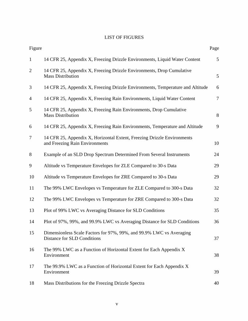
6. Altitude and temperature envelope:

Figure 3. 14 CFR 25, Appendix X, Freezing Drizzle Environments, Temperature and Altitude

6

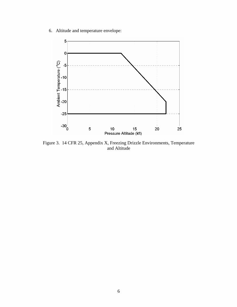
b. Freezing Rain Environments (Conditions with spectra maximum drop diameters greater than 500 µm)

1. Pressure altitude range: 0 to 12,000 ft MSL

2. Maximum vertical extent: 7,000 ft

3. Horizontal extent: standard distance of 17.4 nautical miles (32.2 km)

4. Liquid water content (cloud and precipitation)

Note: LWC based on horizontal extent standard distance of 17.4 nm (32.2 km).

Figure 4. 14 CFR 25, Appendix X, Freezing Rain Environments, Liquid Water Content

7

5. Drop Diameter Distribution

Figure 5. 14 CFR 25, Appendix X, Freezing Rain Environments, Drop Cumulative Mass Distribution

8

6. Altitude and temperature envelope:

Figure 6. 14 CFR 25, Appendix X, Freezing Rain Environments, Temperature and Altitude

9

10

c. Horizontal extent The liquid water content for freezing drizzle environments and freezing rain environments for horizontal extents other than the standard 17.4nm (32.2 km) can be determined by the value of the liquid water content determined from figure 1 or figure 4, multiplied by the factor provided in figure 7.

Figure 7. 14 CFR 25, Appendix X, Horizontal Extent, Freezing Drizzle Environments and Freezing Rain Environments

3. TECHNICAL BASIS FOR PROPOSED APPENDIX X.

3.1 SUMMARY OF FIELD PROJECTS USED FOR PROPOSED APPENDIX X.

The data that were included in the final analysis for the proposed Appendix X came from six field projects conducted by EC and the NASA GRC Icing Technology Branch from 1995 through 2000. These field projects included: • The First Canadian Freezing Drizzle Experiment (CFDE I), which was conducted by EC

in March 1995.

• The Third Canadian Freezing Drizzle Experiment (CFDE III), which was conducted by EC from December 1997 to February 1998.

• The First International Satellite Cloud Climatology Project (ISCCP) Regional

Experiment Arctic Cloud Experiment (FIRE.ACE), which was conducted by EC in April 1998.

• The First Alliance Icing Research Study (AIRS I), which was conducted by EC from

December 1999 and February 2000. • The First Alliance Icing Research Study (AIRS I NASA), which was conducted by

NASA GRC in December 1999. • The SLD Flight Research Study, which was conducted by NASA-Glenn from January

1997 through February 1998.

With the exception of FIRE.ACE, each project was specifically designed to gather in situ observations with instrumented research aircraft in environments where SLD was forecasted to exist. The instrumentation on the aircraft was specifically oriented to adequately measure the SLD environment including the drop distribution and LWC of the entire drop spectrum. While this objective was not inherent to the FIRE.ACE project, this project followed the CFDE III project closely, and the same instrumentation suite was employed. Hence, FIRE.ACE was considered a viable project for adequately measuring SLD conditions. 3.2 FIELD PROJECT THAT ORIGINATED THE EC SLD PROGRAM.

The origin of these projects can be traced, in part, to the Second Canadian Atlantic Storms Program (CASP II), which was conducted by EC from January to March 1992. During CASP II, there were two aircraft icing research objectives: (1) to investigate the microphysical and dynamic properties of East Coast winter storms and the corresponding potential for aircraft icing within such storms, and (2) to determine techniques for validating and improving icing forecasting models. There was no specific objective to measure SLD environments; however, during four research flights, the aircraft encountered regions of supercooled drops between 0.1 and 1 mm in diameter. Two of these encounters were described as “severe icing” by the pilots.

11

A common characteristic of each severe icing encounter was that there was no warm (>0°C) region aloft, implying that the supercooled drops formed through a condensation, coalescence, collision process. This process is also referred to as a warm rain process or as a nonclassical formation process. Unfortunately, the instrumentation suite on the aircraft during CASP II was not considered sufficient for adequately characterizing the SLD environments observed. This was because there was no total water content (TWC) measurement probe, the liquid water hot wire measuring probes had a known fall off for large drops, there was only one Forward Scattering Spectromoter Probe (FSSP) on the aircraft and it was set to measure drops only up to 47 μm in diameter, and the two-dimensional (2D) probes did not always work correctly. Following CASP II, EC researchers proposed that a follow-on field project should be conducted in same geographic region (based from St. John’s, Newfoundland on the Canadian east coast) with the objective of targeting SLD formation regions. This was the origin of the proposal for CFDE I. The proposal was accepted and CFDE I was conducted in March 1995. The Roselawn accident (Marwitz, et al. (1997)), which occurred in October 1994, in which SLD conditions were determined to be a contributing factor, provided considerable impetus to expand the CFDE I research program into CFDE III, the NASA SLD Flight Research Program, and the AIRS projects. The aircraft icing environments encountered during CASP II are described in Cober, et al. (1995). A case study of one of the SLD encounters observed in CASP II is described in detail in Cober, et al. (1997). 3.3 FIELD PROJECTS USED FOR APPENDIX X.

Background information for each of the six field projects is summarized in this section. 3.3.1 CFDE I.

CFDE I was conducted from 1 to 25 March 1995. It was based from St. John’s, Newfoundland, Canada and consisted of 12 research flights into winter storms where freezing precipitation conditions were forecast to exist. St. John’s was chosen as the center for operations because it receives in excess of 150 hours per year of freezing precipitation (McKay and Thompson 1969, Stuart and Isaac 1999). The peak frequency occurs in February and March when an average of 30 hours per month of freezing precipitation is observed at the surface. The unexpected high frequency SLD observations during CASP II combined with the realization that such conditions were reported to be particularly dangerous for aircraft (Sand, et al. (1984), Politovich 1989) led to the proposal for CFDE I, where flights specific to freezing precipitation research were anticipated. A primary research objective of CFDE I was to characterize the aircraft icing environments associated with freezing precipitation, with a view to providing measurements that could be used to help redefine the existing icing envelopes. This was to be achieved by making extensive in situ microphysics measurements in regions where freezing precipitation was forming, with emphasis on regions where the nonclassical formation mechanism was predominant. Nonclassical formation refers to the formation of drops larger than 50 μm in diameter through a

12

condensation and collision-coalescence process. CFDE I has been described by Isaac, et al. (1999, 2001a) and Cober, et al. (2001a). 3.3.2 CFDE III.

CFDE III was conducted between 11 December 1997 and 18 February 1998. The research aircraft was based out of Ottawa, Ontario, Canada, and 26 flights were conducted into winter storms over southern Ontario, southern Quebec, Lake Ontario, and Lake Erie. The geographical region was selected for two reasons: (1) to obtain data in a continental region where there was considerable air traffic and (2) the region around Ottawa and Montreal has a high frequency of freezing precipitation with 50 to75 hours per year observed at the surface (Stuart and Isaac, 1999). The research objectives were essentially the same as for CFDE I. This project has been described by Isaac, et al. (1999, 2001a) and Cober, et al. (2001a). 3.3.3 FIRE.ACE.

FIRE.ACE was conducted between 1 to 29 April 1998. The main goal of this project was to examine the effects of clouds on radiation between the surface, atmosphere, and space, and to study how the surface influences the evolution of boundary layer clouds. The research aircraft was based out of Inuvik of the Northwest Terrorities, Canada, and 18 flights were conducted into boundary layer and mid-level Arctic clouds. The project has been described by Curry, et al. (2000). Gultepe, et al. (2002) and Gultepe and Isaac (2004) describe the LWC and drop concentration measurements made using the Convair-580 during this project. 3.3.4 AIRS I.

AIRS I was conducted between 29 November 1999 and 19 February 2000. The primary objectives of the project were (1) to improve our ability to remotely sense aircraft icing regions using satellite, aircraft, or ground-based systems; and (2) to obtain additional data to characterize the icing environment, particularly icing associated with SLD. AIRS I was based from Ottawa, Ontario, Canada, and the majority of research flights were conducted in the vicinity of Mirabel, Quebec, where a variety of remote sensing instruments were located. There were 25 flights conducted with the National Research Council Convair-580 aircraft during AIRS I. The project has been described by Isaac, et al. (2001 a, b) and Cober, et al. (2002). Isaac, et al. (2001b) present four cases studies describing some of the extreme icing environments encountered during AIRS. 3.3.5 AIRS I NASA.

The NASA GRC Icing group also participated in AIRS I and conducted 16 flights with their Twin Otter research aircraft. Their objectives were the same as described above for AIRS I. Because the Twin Otter was more quickly deployable than the Convair-580 aircraft, its flights tended to be directed towards existing SLD conditions, while the Convair-580 flights were directed toward forecast SLD conditions. The project has been described by Isaac, et al. (2001a, b) and Cober, et al. (2002).

13

3.3.6 NASA SLD Study.

In response to the 1997 FAA In-flight Aircraft Icing Plan, which identified a shortfall in the amount of good quality in situ SLD observations in the Great Lakes region, the NASA Glenn Icing Group, in collaboration with NCAR and the FAA, undertook a multiyear measurement program to acquire additional in situ SLD observations around the lower Great Lakes. The technical objectives of this project included: (1) characterization of the SLD environments, (2) development of improved SLD diagnostic weather forecasting tools, (3) extension of icing simulation capabilities, and (4) provision of educational information about SLD to pilots and the flying community. Flights were specifically targeted at environments nowcasted and forecasted by NCAR specialists to be SLD environments, and between 15 January 1997 and 25 March 1998, they conducted 37 research flights with their Twin Otter research aircraft. The project has been described by Miller, et al. (1998). 3.4 INSTRUMENTATION.

Common instruments were mounted on the Convair-580 research aircraft during CFDE I, CFDE III, FIRE.ACE, and AIRS I. These include two King hot-wire LWC probes, a Nevzorov hot-wire LWC probe, a Nevzorov hot-wire TWC probe, a Rosemount Icing Detector (RID), two Particle Measuring System (PMS) FSSPs, a 2D PMS optical array probe (2D-C) for cloud and drizzle drops, a 2D PMS gray optical array probe (2D-G), a PMS 2D precipitation particle imaging probe (2D-P), and two Rosemount temperature probes. The instruments were mounted on three underwing pylons, including a dedicated pylon for the LWC probes and two pylons that could each hold four PMS-type probes. The NASA Glenn Twin Otter research aircraft flew with a similar instrumentation suite for AIRS I and the NASA SLD Study, although there were fewer duplicate instruments. Its instruments included a King LWC probe, Nevzorov LWC and TWC probe, FSSP, 2D-G, RID, and Rosemount temperature probe. The temperature, LWC, and RID instruments were mounted on the forward fuselage, while the FSSP and 2D probes were mounted on small underwing pylons. Table 1 summarizes the instruments on each aircraft that were used for developing Appendix X. The measurements associated with each instrument will be described below, along with the accuracy, sensitivity, references, and known limitations. It should be noted that each aircraft also carried various additional instruments, which changed from project to project, including aerosol measuring probes, photographic equipment, icing cylinders, prototype SLD detectors, advanced cloud particle imaging probes, dew point hydrometeors, and others. However, since the latter instruments were not used in the analysis of Appendix X conditions, they will not be discussed further in this report.

14

Table 1. Summary of Instruments Used for the Development of Appendix X

NRC Convair-580 Aircraft NASA Glenn Twin Otter Aircraft Rosemount temperature probe Rosemount temperature probe PMS King LWC probe (x2) PMS King LWC probe Nevzorov LWC/TWC probe Nevzorov LWC/TWC probe Goodrich RID Goodrich RID PMS FSSP 3-45 μm PMS FSSP 5-95 μm PMS FSSP 5-95 μm PMS 2D-C 25-800 μm (mono probe) PMS 2D-G 25-1600 μm (grey probe) PMS 2D-G 15-960 μm (grey probe) PMS 2D-P 200-6400 μm (mono probe)

3.4.1 King LWC Probe.

Calibration of the Atmospheric Environment Service (AES) (part of EC prior to 2000) and other King hot-wire LWC probes in a high-speed wind tunnel has been described by King, et al. (1985). Through comparison with icing cylinder measurements, they determined that the King probes collectively had an estimated error of ±15% for droplets <30 μm in diameter. King, et al. (1985) further concluded that the probe response to liquid water is stable over long periods, and that since this response can be calculated directly, the need for frequent wind tunnel calibrations is eliminated. Strapp, et al. (2000) verified that the EC instruments remained stable over a long period of time and continued to measure LWC within ±15%. Removal of the instrument dry power was performed in a manner similar to that suggested by King, et al. (1978). Baseline drift resulting from imperfect dry power removal was estimated by King, et al. (1978) as less than 0.03 g m-3, which agrees with EC observations during CASP II, CFDE I, and CFDE III (Cober, et al. (1995), Cober, et al. (2001b)). To minimize the errors caused by this drift during research flights, the output was artificially zeroed for FSSP concentrations less than 1 droplet cm-3. The data from each flight were carefully examined to ensure that the baseline drift did not exceed 0.02 g m-3, and poor data regions identified were screened out. Cober, et al. (1995) compared LWCs for the two AES King probes mounted side-by-side on the Convair-580 during CASP II and showed that they agreed to within ±15% for 85% of the LWC measurements, although the scatter was significantly higher for LWCs lower than 0.1 g m-3. The increased scatter at lower LWCs is presumably caused by uncertainties in the baseline removal and in the response of the probes to ice crystals. On the Convair-580 aircraft, the King LWC, Nevzorov LWC, and TWC instruments were all mounted on the LWC pylon, which also included a Rosemount temperature probe and a pitot tube. The LWC pylon was situated to hold the instruments ahead of the leading edge of the wing to minimize flow effects associated with airflow around the wing. Flow effects were calculated

15

following Drummond and MacPherson (1985), and the correction factors for all LWC measurements were determined to be between 1.03 and 1.05. Biter, et al. (1987) showed that the response of the King probe was poor for droplets larger than approximately 50 μm in diameter. This was verified and quantified more accurately by Strapp, et al. (2003) who showed that the King probe experienced a 70%, 60%, and 45% underestimate of the LWC for MVD of 50, 100, and 200 μm, respectively. Hot-wire LWC probes respond to ice crystals and this response must be understood to correctly interpret the LWC observed in mixed phase clouds. The interpretation technique is given in Cober, et al. (2001b) and requires the Nevzorov probes; this is discussed in the next section. Without application of this technique, the response to ice water content (IWC) could be interpreted incorrectly as an LWC signal. Cober, et al. (2001b) showed that in glaciated clouds observed with the Convair-580 aircraft at true air speeds of approximately 100 m s-1, where the actual LWC is zero, and the average LWC response is 19% of the IWC for the Nevzorov probe and 15% for the King probe. Strapp, et al. (1999) found that the Nevzorov and King LWC probes showed a 40% response to IWC in glaciated conditions. However, their aircraft flew at 200 m s-1, and the clouds they measured were primarily thunderstorm anvils with high concentrations of small ice particles. The fractional response of the hot-wire LWC instruments to ice crystals is probably dependent on the air speed of the research aircraft and the size of the ice crystals being measured (Strapp, et al. (1999)). 3.4.2 Nevzorov TWC/LWC Probe.

The Nevzorov LWC and TWC probes have been described by Korolev, et al. (1998). The Nevzorov TWC probe measures the sum of LWC and IWC. Comparisons with icing cylinders and King probe measurements in high-speed wind tunnel experiments have shown that the instruments were capable of measuring LWC and TWC, respectively, within 15% with a sensitivity of 0.003-0.005 g m-3. During the research flights in CFDE I, CFDE III, FIRE.ACE, and AIRS I, the Nevzorov zero levels were constantly adjusted to minimize baseline drift. During the post project analysis, the Nevzorov data were further examined to remove any errors associated with baseline drift. Comparisons among the King LWC and Nevzorov LWC and TWC measurements are given in Cober, et al. (2001b). They showed that the LWC measurements agreed within ±15%, with no significant systematic biases for either instrument, when the droplet distributions contained insignificant mass in drops >100μm in diameter; i.e., fewer than 10 drops >100 μm in diameter during a 30-second period. Similar to the King probe, the Nevzorov LWC probe increasingly underestimates the LWC associated with drops >40 μm (Biter, et al. (1987), Strapp, et al. (2003)). Strapp, et al. (2003) showed that the Nevzorov LWC probe experienced a 70%, 60%, and 50% underestimate of the LWC for MVDs of 50, 100, and 200 μm, respectively. Conversely, the Nevzorov TWC probe was designed to minimize this effect (Korolev, et al. (1998)). This was confirmed by Strapp, et al. (2003) who showed that the Nevzorov TWC probe measured the LWC within 30% of calibrated wind tunnel values for MVDs up to 250 μm. The response of the Nevzorov LWC probe to ice crystals is discussed in section 3.4.1.

16

Since the Nevzorov TWC probe was not believed to underestimate the LWC in SLD environments with MVD values larger than 50 μm, it was used as the primary LWC measurement in SLD conditions. The King and Nevzorov LWC probes were used to confirm consistency of the Nevzorov TWC probe and the FSSPs. In mixed phase clouds, the Nevzorov LWC and TWC measurements were used to determine the actual LWC following the technique outlined in Cober, et al. (2001b). 3.4.3 Rosemount Icing Detector.

The RID is a magnetostrictive oscillation probe with a sensing cylinder 6.35 mm in diameter and 2.54 cm in length. Ice buildup on the sensing cylinder causes the frequency of oscillation to change, which can be related to the rate of ice accretion and hence, the cloud LWC. When ice with a thickness of approximately 0.5 mm has accumulated, a heater melts the ice, which is shed into the air stream. The heater cycle is approximately 5 seconds, and the cylinder normally requires an additional 5-10 seconds to cool down to a temperature where it can begin accreting ice again. A detailed description of the instrument is given in Baumgardner and Rodi (1989). A RID model 871FA221B, manufactured by B.F. Goodrich, was mounted on the Convair-580 for all research flights made during CFDE I, CFDE III, FIRE.ACE, and AIRS I. The RID is a very useful instrument for segregating glaciated and nonglaciated conditions because it has no significant response to ice crystals. Heymsfield and Miloshevich (1989) showed that the 1-second response of their instrument to ice particles was <3 mV s-1, for measurements made in cirrus clouds at temperatures <-40°C. Cober, et al. (2001c) used 30-second averaged observations in midlatitude winter storms to show that the instrument response to ice particles was <2 mV s-1 in 98.5% of the observed glaciated clouds. They also found that 99.6% of the average RID responses in clear air were <2 mV s-1, and concluded that 30-second averaged RID measurements made in clear air and glaciated clouds were indistinguishable. For an aircraft flying at 100 m s-1, which is the characteristic speed of the Convair-580, a 2 mV s-1 signal would correspond to an LWC of approximately 0.002 g m-3 (Cober, et al. (2001c)). This is at or below the minimum LWC threshold for the instrument. The LWC threshold is the LWC for which sublimation balances accretion. Sublimation can occur in a water-saturated environment because of the adiabatic heating associated with the speed of the aircraft. The LWC threshold was estimated to be 0.007 ± 0.010 g m-3 by Cober, et al. (2001c) and theoretically predicted to be between 0.002 to 0.006 g m-3 by Mazin, et al. (2001), for an airplane flying at 100 m s-1. In mixed-phase conditions, Cober, et al. (2001c) found that the RID correlation with LWC was the same as for liquid phase conditions, implying that the ice crystals neither accumulated on the sensing cylinder nor eroded the ice buildup to a measurable degree. Cober, et al. (2001c) concluded that for data averaged at 30-second resolution, glaciated cloud conditions could be inferred when the average RID signal was <2 mV s-1 at temperatures <-5°C. A limitation of the RID is that the combination of dynamic heating and latent heat release from supercooled droplets that are freezing on the sensing cylinder can cause the ice surface temperature to reach 0°C (Ludlam, 1951). The Ludlam limit is dependent on the air speed of the aircraft, LWC, and ambient temperature, and the instrument signal can be unreliable for combinations of LWC and temperature that cause the Ludlam limit to be reached (Baumgardner

17

and Rodi, 1989). Cober, et al. (2001c) used in situ data from CFDE I and CFDE III to infer the temperature at which the Ludlam limit was reached for LWC between 0 and 0.6 g m-3. The results were within 15% of the theoretical formulations of Mazin, et al. (2001). The difference between the two was probably caused by the surface roughness coefficient used by Mazin, et al. (2001). When using the RID to identify glaciated conditions, care must be taken to ensure that the absence of a change in the voltage signal is not associated with a LWC that exceeded the Ludlam limit. In the CFDE data set, such observations were infrequent at temperatures <-4°C. Therefore, the absence of a signal on the RID was used to infer glaciated conditions only for temperatures that were colder than -4°C. 3.4.4 FSSP.

The FSSP instruments were used to determine the sizes and concentrations of cloud drops over various diameter ranges. Two FSSPs were mounted on the Convair-580 aircraft for each field project on which the Convair-580 was deployed. Normally, FSSP serial number 96 was used on the 3-45 μm range, while FSSP serial number 124 was used on the 5-95 μm range. Having two FSSP instruments allowed for redundancy in the event of fogging or malfunction of one of the probes. It also allowed for real-time and post-flight consistency checks. Between research flights, the FSSPs were cleaned and calibrated frequently with glass beads. If calibrations revealed under- or oversizing, a uniform gain change in the response of the probe was assumed, and bin diameters were redefined from simple Mie scattering calculations in a manner similar to that used by the manufacturer to set-up the probe originally. Calibration errors of this sort were usually systematic and largely represented a shift caused by an increased buildup of residue in the optics. Particle concentrations, which were usually low, were corrected for dead time and coincidence following Baumgardner, et al. (1985). The error in measurement of droplet concentration has been estimated at ±20% by Baumgardner (1983). On occasion, the FSSPs fogged during descent, which caused the FSSP LWC measurement to be significantly lower than that of the hot-wire LWC probes. Regions of bad data that were clearly caused by excessive ice buildup or fogging during flight were manually identified and removed from the data set. Cober, et al. (2001b) showed a comparison of concentrations from the FSSP 3-45 μm and FSSP 5-95 μm probes for liquid phase conditions observed in CFDE I and CFDE III. The best fit had a slope of 0.97 with a standard error of 41 cm-3 and a correlation coefficient of 0.94. While the concentration measurements showed good agreement, the relative error and scatter were higher than expected. Baumgardner (1983) estimated that a properly calibrated and corrected FSSP could provide concentration measurements within ±17%, so that two FSSPs should agree within ±24%. For the FSSP data shown in Cober, et al. (2001b), and for concentrations >40 cm-3, only 77% of the data agreed within the expected ±24%.

18

The discrepancies were likely caused by the following effects: • The accumulation of ice on the FSSP. Under some heavier icing conditions observed, the

buildup of ice on the FSSP could distort the airflow into the sample area. • Partial fogging of the instruments caused by changes in altitude. Continuous ascents and

descents were common in the majority of the research flights. The aircraft ascent and descent rates were limited to 300 m minute-1 to minimize fogging; however, it was still observed on some occasions.

• Changing cleanliness of the optics from day to day. The optics were cleaned every few

flights, not after every flight. • Unaccounted for flow effects as described by King (1986). The two FSSPs were

mounted in different locations relative to the wing and hence would experience different errors associated with this effect.

• Ice crystal contamination of the FSSP spectra. This effect is expected to be minimized

for the cases selected for the FSSP comparison because of the careful selection process used in identifying liquid phase cases.

Cober, et al. (2001b) also showed a comparison of the FSSP 3-45 μm LWC versus the Nevzorov LWC for CFDE I and CFDE III data. The best fit had a slope of 1.01 with a standard error of 0.034 g m-3 and a correlation coefficient of 0.95. They suggested that this implied that there was no systematic bias between the LWC measurements. These results were consistent with the error estimates of Baumgardner (1983). Data points where the FSSP significantly underestimates the LWC relative to the Nevzorov LWC could be caused by fogging of the FSSP. A comparison of the FSSP 5-95 μm LWC versus the Nevzorov LWC showed similar results with a best fit of 1.06 and standard error of 0.07 g m-3. Similar results have been demonstrated for other projects such as CASP II (Cober, et al. (1995)). FSSPs respond to ice crystals, and the ice crystal, responses can be incorrectly interpreted as drops. Gardiner and Hallett (1985) showed that PMS FSSP probes responded significantly to ice crystals, while the misinterpretation of drops as ice crystals with 2D-C measurements has been discussed by Rauber and Heggli (1988). Based on mixed-phase conditions observed during CFDE I and CFDE III with ice crystal concentrations of 1-5 L-1, Cober, et al. (2001b) found that the FSSP measurements were assessed to be contaminated by ice particles and hence, unreliable for sizes above 35 μm. This observation was similar for both FSSP instruments and independent of the measurement range used. When the data were averaged over the collective CFDE data set, the FSSP measurements in cloud conditions with ice crystal concentration of 1-5 L-1 were found to have concentrations of particles larger than 35 μm that were up to 10 times the concentrations for conditions with no ice crystals. Cober, et al. (2001b) concluded that the FSSPs should not be used to infer drop spectrum characteristics for diameters larger than 35 μm when the ice crystal concentration measured with the 2D probes exceeded 1 L-1.

19

Flow corrections for the PMS FSSPs (King 1986) were not accounted for because the measurement biases associated with the flow fields (approximately 2%) were significantly less than the probe measurement accuracies (>15%). 3.4.5 2D Imaging Probes.

The 2D Cloud (2D-C and 2D-G) and 2D Precipitation (2D-P) probes were used to provide shape, size, and concentrations for particles within their respective size ranges. The size ranges for these three probes, as indicated by the width of the photodiode array, include 2D-C mono 25-800 μm, 2D-C grey (also called 2D-G) 25-1600 μm, and 2D-P mono 200-6400 μm. The NASA 2D-G photodiodes were 15 μm wide for an array width from 15-960 μm. However, the actual size range that drop size and concentration can be accurately determined is rather different. The first four channels of each 2D probe were discarded because of depth of field uncertainties associated with these channels (Joe and List, 1987, Korolev, et al. (1998)) and because of the significant sizing errors that occur in these channels (Korolev, et al. (1991), Korolev, et al. (1998)). Strapp, et al. (2001) showed that distribution measurement errors for the 2D-C mono, when expressed as sizing errors, were <10% for particles ≥5 pixels (125 μm). The hydrometeor images obtained with the 2D probes were processed following the center-in technique of Heymsfield and Parrish (1978). This technique uses circular geometry computations that allow the effective photodiode width to be at least a factor of two larger than the actual photodiode width. It is important to note that since the technique assumes circular geometry, it is only valid for measuring circular particles such as drops. The data from the 2D-C grey probe were processed using two shadow levels (approximately 40%-50%), simulating a 2D-C monoprobe response, although with a smaller sample volume. When using 2D probes to compute the sizes and concentrations of drops greater than 4 pixels in size (125 μm in diameter for the EC 2D-C probe), care must be taken to separate the images associated with drops and images associated with ice crystals and/or erroneous images. The latter include out of focus images, shattered particle images, zero area images, and other erroneous images that the probes are capable of producing. Prior to 2001, there was no published technique for accurately segregating 2D imagery of circles (that are assumed to be drops) and noncircles (that are assumed to be ice crystals). With the requirement to characterize SLD conditions for the aviation community, EC created such a technique and quantified the associated errors (Cober, et al. (2001b)). Images were separated into circles (drops) and noncircles (ice crystals) using diameter, area, perimeter, and symmetry algorithms described by Cober, et al. (2001b). They showed that in liquid phase conditions at temperatures >0°C, where every image was assumed to be a circular drop, in excess of 85% of the particle images were assessed as circles and hence interpreted correctly as drops. Conversely, in glaciated phase conditions, where every image was assumed to be an ice crystal, between 5% and 40% of the processed particle images were assessed as circles, which could be incorrectly interpreted as drops. The relative fractions of circles and noncircles were strongly dependent on particle size, with particles ≤8 pixels in diameter having the largest potential errors. The larger a particle, the higher the resolution of its shape, and hence the higher the accuracy in

20

distinguishing circles from noncircles. In glaciated clouds, a particle size of 11 pixels was required before the average fraction of circular particles dropped below 0.2. The application of such a technique is necessary if 2D images are to be used for deriving drop spectra associated with SLD conditions. Flow corrections for the PMS 2D probes (King, 1986) were not accounted for because the measurement biases associated with the flow fields (approximately 2%) were significantly less than the probe measurement accuracies (>15%). 3.4.6 Temperature Probes.

On the Convair-580, the ambient static temperature was measured with two de-iced Rosemount temperature probes and a reverse flow temperature probe, which normally agreed within ±1°C. Since LWCs were usually less than 0.5 g m-3, errors caused by in-cloud wetting (Lawson and Cooper, 1990) are expected to be less than 0.4°C. Dew point was measured within ±2°C with a Cambridge dewpoint hygrometer. 3.5 REQUIREMENTS FOR CHARACTERIZING SLD ENVIRONMENTS.

The 14 CFR Part 25, Appendix C provides a characterization of aircraft icing environments, with envelopes that incorporate temperature, droplet mean effective diameter (MED), and LWC. As discussed by Lewis (1951), MED is approximately equal to the MVD. The MVD is more commonly used to characterize icing environments. Continuous maximum icing conditions are defined in 14 CFR Part 25, Appendix C as representing extreme icing environments with a horizontal distance of 17.4 nmi (32.2 km). For a given temperature-LWC-MVD point on the envelopes, there is some confusion regarding the probability of simultaneously observing temperatures that are colder, LWC values that are larger, and MVD values that are larger. Simultaneous exceedance probabilities of 0.01 and 0.001 have commonly been associated with these envelopes; however, these may have been based on misinterpretation of the original analysis and may be erroneous. As a starting point for characterizing SLD environments in support of the development of Appendix X, the following measurements were considered essential: • Temperature • Pressure • Horizontal distance • LWC of the entire drop and SLD distribution • Drop size and concentration of the entire drop and SLD distribution Temperature, pressure, and horizontal distance are standard measurements that are easily made to a high level of accuracy. Temperature was normally measured with two or more instruments within an accuracy of ±1°C; pressure was normally measured with two or more pitot tubes within an accuracy of ±0.1 pressure altitude (Pa); and horizontal distance was computed from knowledge of the aircraft true air speed combined with a fixed averaging interval over which the observations were made.

21

Measurements of the LWC and the drop spectrum in an SLD environment are rather difficult to make and require specialized instruments and analysis techniques. Since the standard hot-wire probes were capable of measuring the LWC of non-SLD icing environments to an accuracy of 15 to 20%, it was considered desirable to measure the LWC of the entire SLD spectrum with an accuracy better than 20%. As discussed above, this was achievable with the Nevzorov TWC measuring instrument. No other hot-wire probes (King, Nevzorov LWC, pre-2000 Johnson-Williams) were assessed as being suitable for accurately measuring the LWC in an SLD environment. Similarly, no combination of FSSP, 2D, and/or other spectra measuring probes were capable of measuring LWC in SLD conditions with an accuracy of 20%. For the drop spectrum measurements, since the drop size and concentrations for non-SLD environments could be measured with instruments such as the FSSP and 2D probes with a sizing and concentration accuracy of better than 20%, it was considered desirable to measure the sizes and concentrations of the entire SLD spectrum with the same accuracy. From these measurements, the LWC could be computed for comparison with the LWC derived from hot-wire instruments, and any characteristic diameter, such as MVD, could be inferred. This could be accomplished reasonably well through a combination of FSSP and 2D probes, with a small gap between the maximum measured diameter of the FSSP (95 microns) and the minimum measured diameter of the 2D-C (125 microns). However, the successful application of FSSP and 2D probes to this measurement depended on ice crystal biases being screened out of the FSSP measurements and on an accurate assessment of circles and noncircles on the 2D probes as discussed in Cober, et al. (2001b). When characterizing SLD environments using Nevzorov LWC/TWC, FSSP, and 2D probes, the importance of screening out conditions where ice crystals were significantly biasing the measurement signals from each of these instruments cannot be underestimated. This was most easily accomplished by identifying liquid phase cloud conditions where there were minimal or no ice crystals present or by identifying mixed-phase cloud conditions (liquid and ice particles coexisting) where the concentrations of ice crystals were small enough that their impact on the observations was considered insignificant. This required the development of a technique for determination of cloud phase. SLD environments that included significant ice crystal concentrations, and that were therefore mixed phase in nature, were identified and analyzed; however, these data were not included in Appendix X. 3.6 IDENTIFICATION OF CLOUD PHASE.

Cober, et al. (2001b) developed a methodology for assessing cloud phase based on the relative responses of the instruments described above to ice and liquid hydrometeors. They were able to delineate the phase for each 30-second in-flight interval as being liquid, mixed, or glaciated. Liquid phase clouds were assessed for temperatures colder than -4°C when the following conditions were met. • Agreement between the Nevzorov LWC and TWC probes were within 15% except in

cases with significant mass in drops larger than 100 μm.

22

• A fraction of processed 2D images that were circular particles was greater than 0.85. (Note: this is the proportion of all accepted particle images that were classified as circular images by passing numerous geometric tests, which are described in detail in the Cober, et al. (2001b)).

• The RID is >2 mV s-1, and the concentration of irregular (i.e., ice crystals) images is <0.1

L-1 as measured with the 2D probes. • There is a visual assessment of very few or no ice crystals in the 2D imagery. For cases where the 2D data showed no particles ≥125 μm, the cloud was assumed to have no significant IWC. This is a reasonable assumption for the midlatitude winter clouds observed, where the temperatures and vapor pressures would cause at least some of the ice crystals to grow rapidly to sizes >100 μm in diameter. For cases with significant drizzle concentrations, the LWC/TWC fraction was not expected to agree within 15% because of the roll-off of the LWC probes to large drops. For conditions at temperatures between 0 and -4°C, the RID threshold of 2 mV s-1 was not used in the phase determination. Mixed-phase conditions for temperatures <-4°C were identified when the instruments collectively demonstrated all the following characteristics: • Nevzorov LWC/TWC between 0.25 and 1.0, • fraction of circular 2D images larger than 125 μm between 0.4 and 0.9, • FSSP concentrations >15 cm-3, • visual assessment that the 2D images contained ice crystals, and • a RID response >2 mV s-1. Cober, et al. (2001b) showed that glaciated cloud conditions at temperatures <-4°C could be assessed under the following conditions: • fraction of circular images on the 2D probes <0.35, • Nevzorov LWC/TWC <0.25, • FSSP concentrations <15 cm-3, • RID <2 mV s-1, and • FSSP MVD >30 μm. 3.7 ANALYSIS OF INDIVIDUAL SLD ENVIRONMENTS.

The data from each flight were averaged in sequential 30-second intervals, corresponding to a horizontal length scale of 2.9 ±0.3 km for the NRC Convair-580 data and 2.1 ±0.2 km for the NASA GRC Twin Otter data. The error represents the standard deviation from the mean. The 30-s averaging scale was chosen because it represented a short averaging scale and a scale that generally allowed sufficient 2D measurements (>100) for statistical significance. The phase of each 30-second data point was determined following Cober, et al. (2001b), as described in section 3.6. For each 30-s data point that was assessed to be liquid-phase or mixed-

23

phase with an ice crystal concentration less than 1 L-1, the entire FSSP spectrum, 2D-C spectra ≥125 μm, and 2D-P spectra ≥1000 μm were used to produce a binned drop spectrum from 3 to 3000 μm. The midpoint diameters of each bin were then used to interpolate the normalized droplet spectrum to 1-micron resolution, from 1 micron to the maximum drop diameter. The interpolation was based on a linear fit between logarithmic diameter and concentration pairs. For regions where the 3-45 and 5-95 μm FSSP measurements overlapped, the 3-45 μm data were used unless they were assessed to have been biased because of icing or fogging. The spectra were interpolated in two locations including (1) between the last FSSP channel (≤95 μm depending on where the spectrum is truncated because of insufficient particle counts) and the first useful 2D-C channel (125 μm), and (2) between the last useful 2D-C channel (which varies depending on where the spectrum is truncated because of insufficient particle counts) and the first useful 2D-P channel (1000 μm). FSSP and 2D channels were required to have 10 counts per 30-s interval before they were used in the analysis. When the number of counts per bin fell below 10, bins were combined until 10 counts were obtained. The spectra were truncated when there were fewer than 10 counts in sizes larger than the last useful bin. The maximum drop diameter (Dmax) for each spectrum was assessed as the midpoint of the last useful bin. Each data point with a temperature ≤0°C and with at least one measurement bin of drops larger than 100 μm in diameter was considered as an SLD environment. For each such SLD environment, the 1 μm drop spectrum was used to compute the LWC, mean, mean volume, median volume, 95%, and 99% mass diameters. An example of an integrated drop spectrum for an SLD environment observed during AIRS I is shown in figure 8.

Figure 8. Example of an SLD Drop Spectrum Determined From Several Instruments

The individual channel observations for each instrument are color coded and shown as dots. The combined bins with a minimum of 10 counts are shown with x. The 1 micron spectrum is shown as a solid line. The MVD for this spectrum is 141 μm and the Dmax for the 1 micron spectrum is 1100 μm. 3.8 DEVELOPMENT OF AN SLD DATABASE.

Based on the discussion and conclusions described above, it was accepted that the SLD database from which Appendix X would be derived should only contain data from projects (1) that had acceptable SLD LWC measurements, (2) that had acceptable SLD drop spectra measurements,

24

(3) for which the cloud phase of each SLD observation was accurately assessed, and (4) for which observations that were biased by ice crystal were identified and corrected or removed. Numerous reports of observed SLD conditions were judged not to meet all four of these criteria and were not included in the SLD database. Each of the six projects described in section 3.1 had suitable instrumentation and were analyzed following the methodology of Cober, et al. (2001a). They were included in the SLD database because they met all four criteria. At the time of writing this report, there are other data that meet the criteria described above but which have not been included in the SLD database. Specifically, these data include four flights with the NASA GRC Twin Otter during the CFDE II, four flights with the NASA GRC Convair-580 during the Canadian Extratropical Hurricane Project, 11 flights with the NASA GRC Convair-580 during AIRS 1.5, 21 flights with the NRC Convair-580 during AIRS II, and 21 flights with the NASA GRC Twin Otter during AIRS II. Unfortunately, these data were not processed following the methodology of Cober, et al. (2001b) in time for incorporation into the analysis of the SLD database. In due course, these data will be included in the SLD database. 3.9 SUMMARY OF THE EC/NASA DATA.

In total, there were 48,301 30-second in-flight data points (approximately 400 hours) collected during the 6 flight campaigns summarized in section 3.3. Of these, 27,497 (57%) data points were assessed as being in-cloud with a TWC >0.005 g m-3. There were 22,263 in-cloud observations (46% of in-flight) with an average static temperature ≤0°C, and 14,199 observations (29% of in-flight) where supercooled liquid water was assessed to exist. These are considered in-icing conditions. There were 10,128 in-cloud in-icing data points with ice crystal concentrations less than 1 L-1 where the drop spectra could be accurately determined. Finally, there were 2,444 observations with an average static temperature ≤0 °C, an average LWC >0.005 g m-3, an ice crystal concentration <1 L-1, an assessment of either liquid or mixed-phase, and drops >100 μm in diameter. The latter data points, which represent 5% of the in-flight observations, represent the SLD database on which Appendix X is based. In summary, the 2444 observations of SLD, averaged at 30-second resolution, which were used in the definition of Appendix X, met the following criteria: • average static temperature ≤0°C,

• average LWC >0.005 g m-3, • ice crystal concentration <1 L-1, and • the drop spectrum contains at least 10 drops with diameter >100 μm, which corresponds

to an SLD drop concentration of approximately 0.08 to 0.09 L-1.

25

3.10 INITIAL CONCEPT FOR APPENDIX X.

The 1997 FAA In-flight Aircraft Icing Plan recommended consideration of a comprehensive redefinition of the current aircraft icing certification envelopes when sufficient information was available worldwide on SLD and other icing conditions. Several different characterization approaches for SLD and/or aircraft icing environments have been reported, including 14 CFR Part 25, Appendix C; Newton (1978); Jeck (1996); Politovich (1996); Shah, et al. (2000); and Ashenden and Marwitz (1998), and each of these was considered for Appendix X. Comparisons of in situ data with several of these envelopes have been reported by Cober, et al. (2001a) and Isaac, et al. (2001a). When Appendix X was initially being considered, the aviation community indicated with a fairly strong degree of consensus that 14 CFR Part 25, Appendix C should remain unchanged, and that Appendix X should represent a characterization of SLD conditions distinct from 14 CFR Part 25, Appendix C. They also indicated that Appendix X should provide characteristics of the SLD environment that could be used by manufacturers and regulatory groups. The decision to leave 14 CFR Part 25, Appendix C unchanged was because all existing certification programs, facilities, and experience was based on certification to 14 CFR Part 25, Appendix C conditions, and there was no identified reason to change Appendix C. To conduct realistic wind tunnel or numerical icing simulation experiments that mimic cloud environments that contain SLD, it is necessary to characterize the data in a form that is both practical and realistic. Practical implies a minimum number of representative drop spectra, while realistic implies that a wide range of natural icing conditions should be included in the characteristic spectra. The majority of reports of SLD measurements have simply presented the spectra that were observed (Politovich 1989, Ashenden and Marwitz 1998, Cober, et al. (1996), with no attempt to reconcile or average different environments. Icing environment characterizations such as Cober, et al. (2001a) have typically followed the bulk microphysics approach of 14 CFR Part 25, Appendix C. Jeck (1996) suggested that reported drop spectra could be averaged together in specific diameter bins (i.e., 50-100 μm, 100-200 μm, etc.). Shah, et al. (2000) suggested that the in situ data could be segregated into distinct subsets by varying two parameters, namely the maximum drop diameter (Dmax) and the drop median volume diameter (MVD). They identified five categories: • MVD <50 μm and Dmax <135 μm, • MVD <50 μm and 135 <Dmax <500 μm, • MVD <50 μm and Dmax >500 μm, • MVD >50 μm and 135 <Dmax <500 μm, and • MVD >50 μm and Dmax >500 μm. The first category referred to data that were presumably equivalent to those in 14 CFR Part 25, Appendix C. The Dmax threshold of 135 μm was based on assuming a Langmuir E distribution for

26

all drop distributions that would fall within 14 CFR Part 25, Appendix C. The Dmax threshold of 500 μm was based on the accepted meteorological definition for distinguishing drizzle and rain. While the thresholds suggested by Shah, et al. (2000) were not all ultimately used in Appendix X, the overall approach was recognized as being potentially useful to the aviation community. After a considerable number of sensitivity studies, and additional analysis (discussed below) it was determined that four SLD conditions similar to those proposed by Shah, et al. (2000) could be used to characterize the entire SLD environment. Hence, this framework was adopted as the foundation of Appendix X. 3.11 DEFINITION OF APPENDIX X.

Appendix X was defined to incorporate all SLD icing conditions in which the Dmax exceeds 100 μm, as explained above. Appendix X spectra can be subdivided into icing environments with maximum drop sizes between 100 and 500 microns, nominally called freezing drizzle environments (ZLE) and icing environments with Dmax >500 microns, nominally called freezing rain environments (ZRE). Each of these environments can be further separated into two conditions, one with MVD <40 µm, and one with MVD >40 µm. The MVD threshold of 40 μm was selected because it represents the maximum MED of 14 CFR Part 25, Appendix C continuous maximum (stratiform clouds) icing conditions. Appendix X conditions are assumed to be distinct from 14 CFR Part 25, Appendix C conditions in that all Appendix X conditions have SLD with maximum diameters >100 μm, while in general, 14 CFR Part 25, Appendix C stratiform conditions are assumed to have Dmax <100 μm. Hence, Appendix C and Appendix X together account for almost all icing environments associated with supercooled liquid water. The term “almost” is used because there is an icing region that is not accounted for by either envelope, namely where the MVD >40 μm and the Dmax is <100 μm. However, this region contained only 90 observations at 30-second resolution, or 4% of all SLD observations on which Appendix X is based, and it is assumed that these conditions are close enough to 14 CFR Part 25, Appendix C conditions that Appendix C can be assumed to adequately describe them. The four subsets of Appendix X conditions are summarized in table 2.

Table 2. Four Subsets of Appendix X Conditions

Definition MVD Dmax

Number of 30-s Data

Points ZLE <40 μm 100-500 μm 1469 ZLE >40 μm 100-500 μm 335 ZRE <40 μm >500 μm 193 ZRE >40 μm >500 μm 447

The threshold maximum drop sizes of 100 and 500 μm were selected to be partly consistent with the meteorological definitions of freezing drizzle and freezing rain. Freezing drizzle is defined

27

in the Glossary of Meteorology as supercooled drops between 200 and 500 μm in diameter, and freezing rain is defined as supercooled drops larger than 500 μm in diameter. Shah, et al. (2000) suggested a value of 135 μm for the threshold between 14 CFR Part 25, Appendix C and Appendix X, based on the assumption that 14 CFR Part 25, Appendix C conditions could be described with a Langmuir E distribution, and a Langmuir E distribution with a MVD of 50 μm would have a Dmax of 135 μm. A sensitivity study using different thresholds between 50 and 150 μm was described by Cober, et al. (2003). They concluded that there were no significant differences in the spectra by using thresholds between 100 and 135 μm. Therefore, a threshold of 100 μm was used for Appendix X. The MVD threshold of 40 μm was selected to be consistent with the limits of 14 CFR Part 25, Appendix C for continuous maximum icing, since this more closely corresponded to conditions in the in situ SLD data collected in the research programs. Cober, et al. (2003) also did a sensitivity study using MVD thresholds of 40 and 50 μm and concluded that the choice of MVD threshold in this range made little difference in the derivation of the Appendix X distributions. Since Appendix X contains all icing environments with Dmax >100 μm, then all Appendix X data were separated from the larger icing database. As discussed in section 3.9, there were 2444 separate observations at 30-second resolution of Appendix X conditions. The number of data points in each Appendix X subset is also shown in table 2. These data were used to define parameters relating to Appendix X including pressure altitude, vertical and horizontal extent, temperature, LWC, and water mass distribution as a function of drop diameter distribution. 3.12 BULK CHARACTERISTICS OF APPENDIX X.

The discussion in this section provides the justification for the values stated in the proposed Appendix X for pressure altitude range, maximum vertical extent, and horizontal extent for freezing drizzle and freezing rain. Figure 9 shows a plot of pressure altitude versus temperature for all Appendix X ZLE conditions. The data are separated into ZLE with MVD <40 μm and ZLE with MVD >40 μm. Figure 10 shows a similar plot for the Appendix X ZRE conditions. Temperature versus pressure altitude envelopes were derived based on the observed data and on similar envelopes given in 14 CFR Part 25 Appendix C. It was found that the latter envelopes entirely bounded the observed ZLE and ZRE conditions. The envelopes are overlaid on figures 9 and 10 and appear in figures 3 and 6, respectively, of the proposed Appendix X. There are a few ZRE data points that are outside the ZRE envelope. These represent SLD conditions that formed drops larger than 500 μm in diameter through a collision coalescence process. For this reason, and notwithstanding the maximum drop size, these data were considered to be more representative of ZLE conditions than ZRE. The ZLE envelope captures these data sufficiently.

28

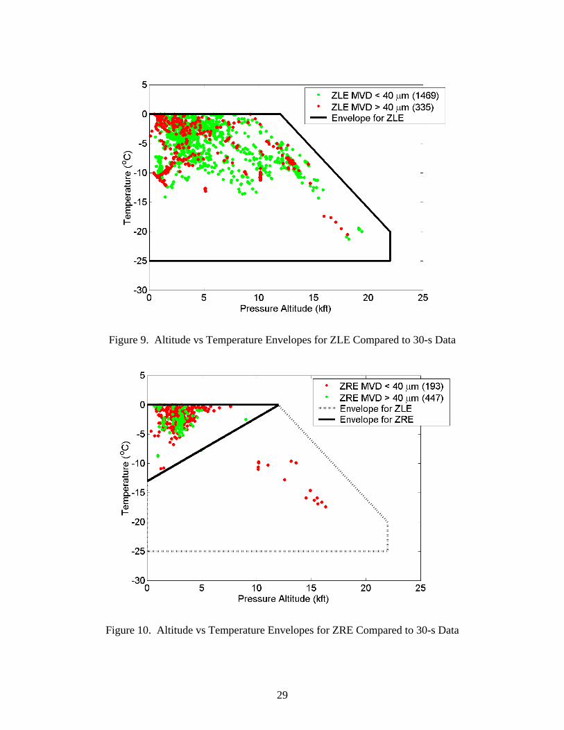
Figure 9. Altitude vs Temperature Envelopes for ZLE Compared to 30-s Data

Figure 10. Altitude vs Temperature Envelopes for ZRE Compared to 30-s Data

29

Based on the in situ observations, and in the absence of any freezing drizzle observations colder than -25°C, it was concluded that the probability of ZLE conditions existing in the natural atmosphere at ambient temperatures colder than -25°C was negligible. Similarly, it was concluded that the probability of ZRE conditions existing in the natural atmosphere at ambient temperatures colder than -13°C was negligible. All Appendix X conditions were related to a standard horizontal extent of 17.4 nmi to be consistent with the standard distance for continuous maximum clouds of 14 CFR Part 25, Appendix C. The derivation of Appendix X LWC values at a horizontal extent of 17.4 nmi will be discussed in section 3.13. The maximum vertical extents of Appendix X freezing drizzle and rain conditions were estimated from the in situ observations. Based on all flights in the FAA master database, including the 134 research flights that were undertaken to collect the SLD data on which Appendix X is based, the largest observed vertical extent of a freezing drizzle condition was 12,000 feet, while the largest observed vertical extent of a freezing rain condition was 7,000 feet. Since similar vertical extents were estimated in the sounding-based inferred SLD climatology, these values were selected to characterize ZLE and ZRE conditions within Appendix X (Bernstein 2005 and 2009 and Bernstein, et al., 2003). 3.13 THE LWC CHARACTERISTICS OF APPENDIX X.

The determination of the LWC characteristics of Appendix X involved several distinct analytical steps, which are summarized here. The details of each step are outlined in several subsequent sections. The sequence of the LWC analysis was as follows: a. The SLD data were averaged for averaging periods of 30-s, 60-s, 120-s, and 300-s

corresponding nominally to horizontal extents of 3, 6, 12, and 30 km, respectively. The 30-s analysis was described in section 3.9. The 60, 120, and 300-s analysis are described in section 3.16.

b. Each individual SLD data point for each averaging period was normalized to a constant

temperature of 0°C. The normalization methodology is discussed in section 3.14. c. For each of the four averaging periods, the 0°C normalized LWC values for all SLD

environments observed were used to assess the 99% LWC, value using an extreme value analysis procedure described in section 3.21.

d. The 99% LWC values for the four averaging periods were used to derive a single SLD

scale factor (SF) equation that relates horizontal extent to 99% LWC as described in section 3.16.

e. Using the 0°C normalized LWC values for each of the four SLD subsets (two freezing

drizzle environments and two freezing rain environments), the 99% LWC values were determined for each of the four averaging periods using an extreme value analysis procedure described in section 3.21.

30

f. For each of the four SLD subsets, the SLD SF described in step 4 was fit by eye to match the 99% LWC versus horizontal extent by varying the y intercept. This is shown in section 3.16.

g. Using each of the four SF equations determined in step 6 above, which correspond to the

four SLD subsets respectively, the 99% LWC value was computed for a horizontal extent of 17.4 nmi (32.2 km) for each SLD subset. These values are assumed to be valid for 0°C since they were based on data that were normalized to 0°C. This is shown in section 3.16, and the results are listed in table 3.

h. The 99% LWC values at 0°C and 17.4 nmi for each SLD subset were computed for

colder temperature values by assuming that the atmospheric temperature-pressure relationship followed the U.S. standard atmosphere. The assumptions and methodology are given in section 3.15, and the results are shown in figures 11 and 12.

The maximum LWC values for each Appendix X condition for a horizontal extent of 17.4 nmi for a temperature of 0°C are summarized in table 3. These maximum LWC values represent the 99% exceedance values for SLD conditions. This implies that for any given icing condition (temperature ≤0°C) with a maximum drop size >100 μm, and is therefore assessed to be an Appendix X condition, 99% of all such conditions will have an LWC of less than the exceedance value listed in table 3.

Table 3. Maximum LWC for Appendix X Conditions

Definition MVD Dmax Maximum LWC ZLE <40 μm 100-500 μm 0.44 g m-3 ZLE >40 μm 100-500 μm 0.27 g m-3 ZRE <40 μm >500 μm 0.31 g m-3 ZRE >40 μm >500 μm 0.26 g m-3

Figure 11 shows a plot of temperature versus LWC for Appendix X freezing drizzle environments. The values of LWC shown are valid for the reference distances of 17.4 nmi (32.2 km). The data are segregated into ZLE with MVD <40 μm and ZLE with MVD >40 μm. Figure 12 shows a similar plot for the Appendix X freezing rain environments.

31

Figure 11. The 99% LWC Envelopes vs Temperature for ZLE Compared to 300-s Data

Figure 12. The 99% LWC Envelopes vs Temperature for ZRE Compared to 300-s Data

32

3.14 NORMALIZATION OF THE DATA TO 0°C.

For each averaging period and for each SLD subset, to determine the 99% LWC values for a temperature of 0°C, the individual LWC values used in the analysis were first normalized to a standard temperature of 0°C. The normalization was done by assuming that the liquid water mixing ratio would remain constant for any change in temperature or pressure. The liquid water mixing ratio physically represents the mass of liquid water per unit mass of air. Starting with an observed temperature and pressure, assuming that the pressure did not change so that Pobs = P0C, and assuming that the mixing ratio remained constant, the following equation could then be applied

00

0

ρ( , )[ ] [ρ( , )

C obs obsC obs obs

obs obs C

T P TLWC LWC LWCT P T

= = ]

where LWC is the liquid water content, ρ the density of dry air, T the temperature and P the pressure. The subscript “obs” refers to the value of the parameter observed and the subscript “0C” refers to the value of the parameter at 0°C. Since Tobs and T0C were normally within 5% of each other, the normalization of the data to 0°C had a mimimal effect on the analysis. It is important to note that no normalization was done with respect to pressure for the observed data, hence the assumption that Pobs = P0C. Once the data were normalized to 0°C, the 99% LWC values were determined by extreme value analysis, as described in section 3.21. 3.15 COMPUTATION OF LWC VARIATION WITH TEMPERATURE.

Based on the 99% LWC value assessed at 0°C, the LWC temperature curves shown in figures 11 and 12 were computed using the following methodology. The mean temperature and pressure of all the 30-s SLD data observed was -4.2°C and 865 mb, respectively. These values were used to modify the U.S. standard atmosphere, which provides a relationship between temperature and pressure, so that the U.S. standard atmosphere temperature at 865 mb was also equal to -4.2°C. The modification required was a systematic reduction of the temperature profile by 11.0°C, which represents a cooler atmosphere than the U.S. standard atmosphere. This is consistent with the winter nature of the SLD observations. The modified U.S. standard atmosphere equation for computing pressure from temperature is

2577.5]0.1115.288[0.101325 −−=

TP

where P is the pressure in Pascals and T is the temperature in Kelvin. The 11.0°C modification can be clearly seen in the equation. Selected values of temperature and pressure for the modified U.S. standard atmosphere are given in table 4. These can be computed from the previous equation.

33

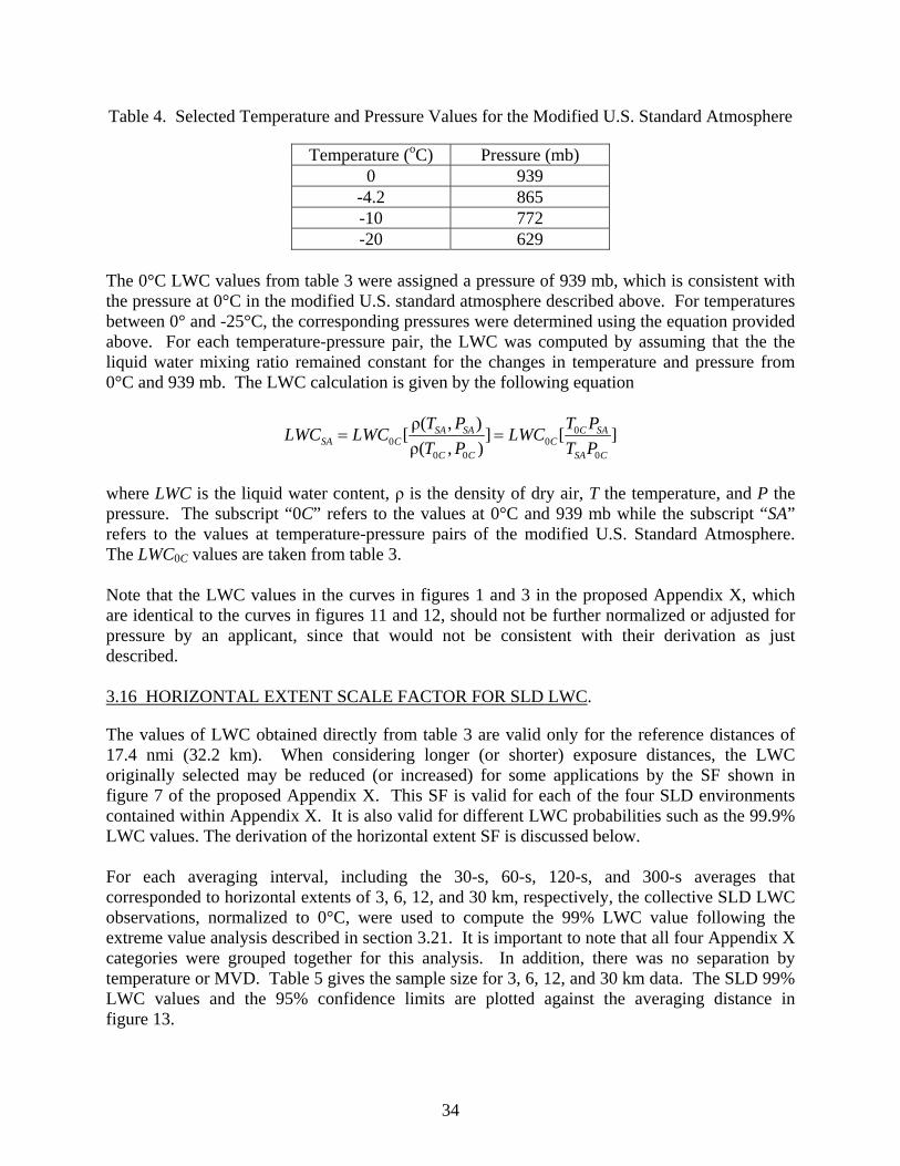
Table 4. Selected Temperature and Pressure Values for the Modified U.S. Standard Atmosphere

Temperature (oC) Pressure (mb) 0 939

-4.2 865 -10 772 -20 629

The 0°C LWC values from table 3 were assigned a pressure of 939 mb, which is consistent with the pressure at 0°C in the modified U.S. standard atmosphere described above. For temperatures between 0° and -25°C, the corresponding pressures were determined using the equation provided above. For each temperature-pressure pair, the LWC was computed by assuming that the the liquid water mixing ratio remained constant for the changes in temperature and pressure from 0°C and 939 mb. The LWC calculation is given by the following equation

00 0

0 0 0

ρ( , )[ ] [ρ( , )

SA SA C SASA C C

C C SA C

T P T PLWC LWC LWCT P T P

= = ]

where LWC is the liquid water content, ρ is the density of dry air, T the temperature, and P the pressure. The subscript “0C” refers to the values at 0°C and 939 mb while the subscript “SA” refers to the values at temperature-pressure pairs of the modified U.S. Standard Atmosphere. The LWC0C values are taken from table 3. Note that the LWC values in the curves in figures 1 and 3 in the proposed Appendix X, which are identical to the curves in figures 11 and 12, should not be further normalized or adjusted for pressure by an applicant, since that would not be consistent with their derivation as just described. 3.16 HORIZONTAL EXTENT SCALE FACTOR FOR SLD LWC.

The values of LWC obtained directly from table 3 are valid only for the reference distances of 17.4 nmi (32.2 km). When considering longer (or shorter) exposure distances, the LWC originally selected may be reduced (or increased) for some applications by the SF shown in figure 7 of the proposed Appendix X. This SF is valid for each of the four SLD environments contained within Appendix X. It is also valid for different LWC probabilities such as the 99.9% LWC values. The derivation of the horizontal extent SF is discussed below. For each averaging interval, including the 30-s, 60-s, 120-s, and 300-s averages that corresponded to horizontal extents of 3, 6, 12, and 30 km, respectively, the collective SLD LWC observations, normalized to 0°C, were used to compute the 99% LWC value following the extreme value analysis described in section 3.21. It is important to note that all four Appendix X categories were grouped together for this analysis. In addition, there was no separation by temperature or MVD. Table 5 gives the sample size for 3, 6, 12, and 30 km data. The SLD 99% LWC values and the 95% confidence limits are plotted against the averaging distance in figure 13.

34

Table 5. Sample Size of SLD Conditions for Each Length Scale

Averaging Interval Length Scale Number of Data Points 30-second 3 km 2444 60-second 6 km 1431 120-second 12 km 850 300-second 30 km 460

Figure 13. Plot of 99% LWC vs Averaging Distance for SLD Conditions

The data in figure 13 were fit to a linear best fit as LWC99 = 0.553 – 0.089log10(dHkm) (1)

where dHkm is the horizontal averaging distance in km and LWC99 is the 99% LWC in g m-3 at the averaging distance dHkm. Based on equation 1, at a horizontal extent of 17.4 nmi the LWC is 0.418 g m-3.

35

It is possible to define a dimensionless SF so that equation 1 can be rewritten as follows: LWCd = LWC17.4*SF99 (2) SF99 = (1/0.418)*(0.553 – 0.089 log10(dHkm)) = 1.322 – 0.213 log10(dHkm) (3) where SF99 is the scale factor for the 99% LWC data, and LWC17.4 is the value of LWC99 at a horizontal extent of 17.4 nmi. Note that the SF has been defined so that it is equal to 1 at 17.4 nmi. The dimensionless SF, with a value of 1 at 17.4 n mi, parallels the dimensionless SF in 14 CFR Part 25, Appendix C. Equation 3 can also be expressed in terms of a horizontal averaging distance in nmi (dHnmi) as follows:

SF99 = 1.266 – 0.213 log10(dHnmi) (4)

To determine whether equations 2 and 3 were valid for other low probability LWC values, extreme value analysis was used to compute the 97% and 99.9% LWC values for each of the four averaging periods. The best fits of LWC versus averaging distance are shown in figure 14.

Figure 14. Plot of 97%, 99%, and 99.9% LWC vs Averaging Distance for SLD Conditions

36

When the 97% and 99.9% fits in figure 14 are transformed into dimensionless SFs, such as equation 3, the equations for the SFs are as follows: SF 97 = 1.315 – 0.208 log10(dHkm) (5) SF 99.9 = 1.328 – 0.218 log10(dHkm) (6) where SF97 and SF99.9 are the scale factors for the 97% LWC, and 99.9% LWC data, respectively. These equations are within 3% of equation 3, which suggests that equation 3 is valid for LWC probabilities between 97% and 99.9%. The three dimensionless SFs from figure 14 are plotted in figure 15. The three curves essentially fall on top of each other and cannot be distinguished.

Figure 15. Dimensionless Scale Factors for 97%, 99%, and 99.9% LWC vs Averaging Distance for SLD Conditions

To determine whether equation 3 was valid for each Appendix X environment, extreme value analysis was performed for each horizontal extent for each of the four SLD subsets to assess the 99% LWC values. The 99% LWC values, along with their 95% confidence limits, are shown in figure 16.

37

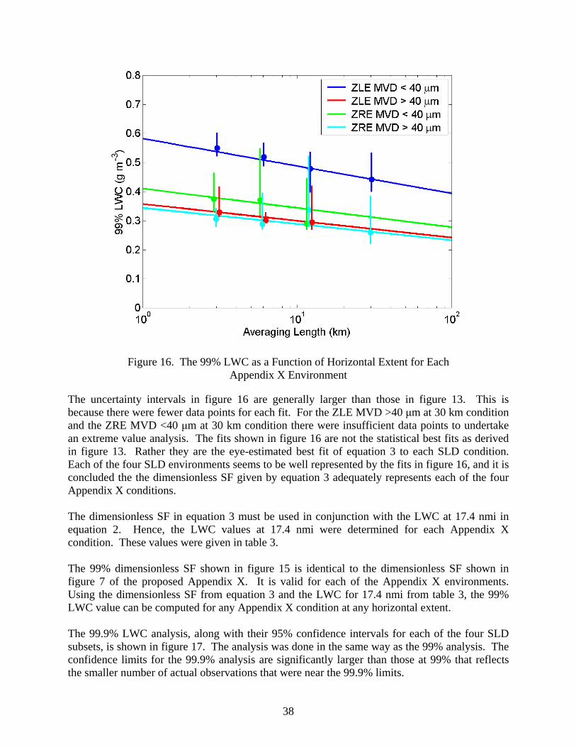
Figure 16. The 99% LWC as a Function of Horizontal Extent for Each Appendix X Environment

The uncertainty intervals in figure 16 are generally larger than those in figure 13. This is because there were fewer data points for each fit. For the ZLE MVD >40 μm at 30 km condition and the ZRE MVD <40 μm at 30 km condition there were insufficient data points to undertake an extreme value analysis. The fits shown in figure 16 are not the statistical best fits as derived in figure 13. Rather they are the eye-estimated best fit of equation 3 to each SLD condition. Each of the four SLD environments seems to be well represented by the fits in figure 16, and it is concluded the the dimensionless SF given by equation 3 adequately represents each of the four Appendix X conditions. The dimensionless SF in equation 3 must be used in conjunction with the LWC at 17.4 nmi in equation 2. Hence, the LWC values at 17.4 nmi were determined for each Appendix X condition. These values were given in table 3. The 99% dimensionless SF shown in figure 15 is identical to the dimensionless SF shown in figure 7 of the proposed Appendix X. It is valid for each of the Appendix X environments. Using the dimensionless SF from equation 3 and the LWC for 17.4 nmi from table 3, the 99% LWC value can be computed for any Appendix X condition at any horizontal extent. The 99.9% LWC analysis, along with their 95% confidence intervals for each of the four SLD subsets, is shown in figure 17. The analysis was done in the same way as the 99% analysis. The confidence limits for the 99.9% analysis are significantly larger than those at 99% that reflects the smaller number of actual observations that were near the 99.9% limits.

38

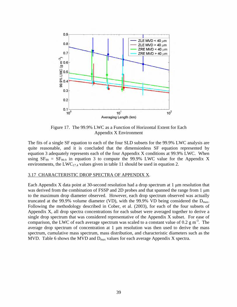
Figure 17. The 99.9% LWC as a Function of Horizontal Extent for Each Appendix X Environment

The fits of a single SF equation to each of the four SLD subsets for the 99.9% LWC analysis are quite reasonable, and it is concluded that the dimensionless SF equation represented by equation 3 adequately represents each of the four Appendix X conditions at 99.9% LWC. When using SF99 = SF99.9 in equation 3 to compute the 99.9% LWC value for the Appendix X environments, the LWC17.4 values given in table 11 should be used in equation 2. 3.17 CHARACTERISTIC DROP SPECTRA OF APPENDIX X.

Each Appendix X data point at 30-second resolution had a drop spectrum at 1 μm resolution that was derived from the combination of FSSP and 2D probes and that spanned the range from 1 μm to the maximum drop diameter observed. However, each drop spectrum observed was actually truncated at the 99.9% volume diameter (VD), with the 99.9% VD being considered the Dmax. Following the methodology described in Cober, et al. (2003), for each of the four subsets of Appendix X, all drop spectra concentrations for each subset were averaged together to derive a single drop spectrum that was considered representative of the Appendix X subset. For ease of comparison, the LWC of each average spectrum was scaled to a constant value of 0.2 g m-3. The average drop spectrum of concentration at 1 μm resolution was then used to derive the mass spectrum, cumulative mass spectrum, mass distribution, and characteristic diameters such as the MVD. Table 6 shows the MVD and Dmax values for each average Appendix X spectra.

39

Table 6. The MVD for Appendix X Conditions

Definition MVD Range Dmax Range

MVD (50% VD)

Dmax (99.9% VD)

ZLE <40 μm 100-500 μm 20 μm 389 μm ZLE >40 μm 100-500 μm 110 μm 474 μm ZRE <40 μm >500 μm 19 μm 1553 μm ZRE >40 μm >500 μm 526 μm 2229 μm

The cumulative mass distribution, as a fraction of the LWC, for each freezing drizzle and freezing rain spectra appear in figures 2 and 5 of the proposed Appendix X. The actual mass distributions for each of the freezing drizzle and freezing rain spectra are shown in figures 18 and 19, respectively. Each of these spectra has an LWC of 0.2 g m-3.

Figure 18. Mass Distributions for the Freezing Drizzle Spectra

40

Figure 19. Mass Distributions for the Freezing Rain Spectra

The normalized mass distributions, representing ∆(LWC)/∆log(Diameter) versus diameter, for each of the freezing drizzle and rain spectra are shown in figures 20 and 21, respectively. The normalization adjusts for the log scale on the horizontal axis in such a way that area is “preserved” in the figures, so that the features, such as bimodality, are readily apparent. Each of these spectra has a LWC of 0.2 g m-3.

41

Figure 20. Normalized Mass Distributions for the Freezing Drizzle Spectra

Figure 21. Normalized Mass Distributions for the Freezing Rain Spectra

42

The bimodal natures of the ZLE and ZRE conditions are clearly evident in these plots. For ZLE MVD <40 μm and ZRE MVD <40 μm conditions, the cloud drop mass peak around 10-20 μm is the dominant one. For ZLE MVD >40 μm and ZRE MVD >40 μm conditions, the dominant peak for mass is in the peak that occurs in the drizzle (around 200-300 μm) or rain size (around 700-800 μm) ranges. In all cases, the large drop peak dominates the reflectivity spectra. Similar observations regarding the reflectivity results were discussed in Isaac, et al. (2002). The wide variation in the cumulative mass curves suggests that the four spectra have distinct characteristics, and that they collectively appear to cover a wide range of naturally observed icing conditions. The formation mechanism for each 30-second SLD data point was assessed as either classical, implying that it formed through a melting and resupercooling mechanism, or nonclassical, implying that it formed through a condensation and collision-coalescence mechanism. For ZLE conditions, 88% were observed to have formed through a nonclassical process. Conversely, for ZRE conditions, 92% were observed to have formed through a classical process. This highlights that the ZLE and ZRE conditions observed are relatively distinct in that they primarily formed through fundamentally different mechanisms in the atmosphere. Figures 22 through 25 show the average cumulative mass spectrum for each Appendix X condition compared to each individual spectra that were used in the averages. These show the variability in the spectra that were used in each average. They also show that each of the four Appendix X conditions seems distinct from the others, so that the four collectively cover the entire SLD environment.

Figure 22. Average Cumulative Mass Spectrum for ZLE With MVD <40 μm, Compared to Each Individual Cumulative Mass Spectra

43

Figure 23. Average Cumulative Mass Spectrum for ZLE With MVD >40 μm, Compared to Each Individual Cumulative Mass Spectra

Figure 24. Average Cumulative Mass Spectrum for ZRE With MVD <40 μm, Compared to Each Individual Cumulative Mass Spectra

44

Figure 25. Average Cumulative Mass Spectrum for ZRE With MVD >40 μm, Compared to Each Individual Cumulative Mass Spectra

3.18 BIN REPRESENTATION FOR APPENDIX X MASS SPECTRA.

In the proposed advisory circular on compliance with the proposed 14 CFR 25.1420 and Appendix X, it is noted that applications of DSDs often require a bin tabulation of the proportion of mass (LWC) relative to drop diameter. The proposed advisory circular presents tables, which are reproduced below as tables 7 and 8, which represent 10-bin tabulations for the cumulative distributions in Appendix X. The mass proportions for the bins were selected to provide reasonable resolution of the upper range of the distributions. The shaded columns (a) and (b) in the tables contain the values that typically would be input to ice accretion computer codes.

45

Table 7. The 10-Bin Drop Distributions for ZLE

ZLE (MVD <40 μm) ZLE (MVD >40 μm) (a) (b) (b)

Bin Proportion

of Mass

Left Boundary

Point (μm)

Mass-Weighted Midpoint

(μm)

Right Boundary

Point (μm)

Left Boundary

Point (μm)

Mass-Weighted Midpoint

(μm)

Right Boundary

Point (μm)

1 0.100 1 9 10 1 11 15 2 0.200 10 13 16 15 22 36 3 0.200 16 18 20 36 66 110 4 0.200 20 23 27 110 155 202 5 0.100 27 29 33 202 227 252 6 0.050 33 35 39 252 266 280 7 0.050 39 46 64 280 296 313 8 0.050 64 96 138 313 333 357 9 0.025 138 166 205 357 373 392 10 0.025 205 254 389 392 419 474

Note: The DSDs in 1-micron drop bin resolution are available in electronic files from the FAA William J. Hughes Technical Center.

Table 8. The 10-Bin Drop Distributions for ZRE

ZRE (MVD <40 μm) ZRE (MVD >40 μm) (a) (b) (b)

Bin Proportion

of Mass

Left Boundary

Point (μm)

Mass-Weighted Midpoint

(μm)

Right Boundary

Point (μm)

Left Boundary

Point (μm)

Mass-Weighted Midpoint

(μm)

Right Boundary

Point (μm)

1 0.100 1 7 8 1 9 14 2 0.200 8 10 12 14 36 239 3 0.200 12 15 19 239 400 526 4 0.200 19 25 51 526 645 766 5 0.100 51 263 470 766 834 912 6 0.050 470 535 595 912 957 1008 7 0.050 595 655 718 1008 1066 1130 8 0.050 718 792 883 1130 1198 1289 9 0.025 883 942 1035 1289 1346 1421 10 0.025 1045 1191 1553 1421 1546 2229

Note: The DSDs in 1-micron drop bin resolution are available in electronic files from the FAA William J. Hughes Technical Center.

These tables were determined directly from the 1-micron resolution DSD for each of the four SLD curves, starting from the 1 micron lower boundary and using the specified proportions of mass and rounding to whole numbers. For example, for ZRE (MVD >40 μm), approximately

46

10% of the mass falls in the interval from 1 μm to 14 μm and approximately half is below 9 μm and half above 9 μm (mass-weighted midpoint). If a different representation is needed using different proportions or a different number of bins, such a representation can be determined in exactly the same manner from the DSDs in 1-micron drop bin resolution.

Figures 26 through 29 are plots the mass-weighted midpoints in tables 7 and 8 on the cumulative mass curves for each of the four distributions. These figures show the resolution achieved for the larger drop diameters by using the bin representations in the tables.

0.00

0.10

0.20

0.30

0.40

0.50

0.60

0.70

0.80

0.90

1.00

1 10 100 1000

Drop Diameter (microns)

Cum

ulat

ive

Mas

s

Cumulative MassDistributionMass-Weighted Midpoints ofBins

Figure 26. Cumulative Mass Distribution and Bin Midpoints in Proposed Advisory Circular for ZLE With MVD <40 μm

0.00

0.10

0.20

0.30

0.40

0.50

0.60

0.70

0.80

0.90

1.00

1 10 100 1000

Drop Diameter (microns)

Cum

ulat

ive

Mas

s

Cumulative MassDistributionMass-Weighted Midpoints ofBins

Figure 27. Cumulative Mass Distribution and Bin Midpoints in Proposed Advisory Circular for ZLE With MVD >40 μm

47

0.00

0.10

0.20

0.30

0.40

0.50

0.60

0.70

0.80

0.90

1.00

1 10 100 1000 10000

Drop Diameter (microns)

Cum

ulat

ive

Mas

s Cumulative MassDistributionMass-Weighted Midpoints ofBins

Figure 28. Cumulative Mass Distribution and Bin Midpoints in Proposed Advisory Circular for ZRE With MVD <40 μm

0.00

0.10

0.20

0.30

0.40

0.50

0.60

0.70

0.80

0.90

1.00

1 10 100 1000 10000

Drop Diameter (microns)

Cum

ulat

ive

Mas

s

Mass-Weighted Midpoints ofBinsCumulative MassDistribution

Figure 29. Cumulative Mass Distribution and Bin Midpoints in Proposed Advisory Circular for ZRE With MVD >40 μm

48

3.19 DERIVATION OF APPENDIX X PRECIPITATION RATES.

The precipitation rate for each SLD spectrum was computed by integrating the 1 μm LWC spectra as given by

RR = ∑ (LWC1* Vt * 3.6)

where RR is the precipitation rate in mm h-1, LWC1 is the LWC of each 1 μm diameter bin in g m-3 and Vt is the terminal velocity in m s-1 for a drop with a diameter equal to the bin diameter. The terminal velocities for drops of diameter D in microns were taken from Yau and Rogers (1989) and are given by

Vt = k 1 (D/2)2, for 1 < D < 60 μm,

where k 1 is 1.19x106 cm-1 s-1

Vt = k 2 (D/2), for 60 < D < 1200 μm,

where k 2 is 9.3x103 s-1

Vt = k 3 (D/2)0.5, for 1200 < D < 4000 μm,

where k3 is 2.01x103 cm-0.5 s-1

Figures 30 and 31 show histograms of precipitation rates for Appendix X ZLE and ZRE conditions, respectively. The thresholds for light, moderate, and heavy ZLE and ZRE conditions are also shown on each histogram for comparison. The fractions of precipitation rates that were classified as light, moderate, and heavy were 0.94, 0.04, and 0.02, respectively for ZLE and 0.98, 0.02, and 0.00, respectively for ZRE. The 99% precipitation rate values were computed for the ZLE and ZRE conditions using a Weibull distribution. They were 0.4 mm h-1 for ZLE and 3.2 mm h-1 for ZRE, both of which are classified as moderate. Appendix X conditions were all observed in and/or below stratiform winter clouds, and it is reasonable to assume that the precipitation rates determined for Appendix X are applicable below cloud to the surface. This is why the pressure altitude envelopes in figures 3 and 6 extend to the surface. This assumption ignores possible evaporation that may occur below cloud, which in turn would reduce the precipitation rate and alter the spectrum.

49

Figure 30. Histogram of Precipitation Rates for ZLE Conditions

Figure 31. Histogram of Precipitation Rates for ZRE Conditions

50

The precipitation rates associated with each of the four distributions and 99% LWC values can also be calculated in the same manner. Using the 1 μm resolution spectra for each Appendix X distribution, precipitation rates were computed for the associated 99% LWC values from table 3. The results are shown in table 9.

Table 9. Precipitation Rates for Appendix X Distributions With 99% LWC Values

Definition MVD Dmax Precipitation Rate ZLE <40 μm 100-500 μm 0.12 mm h-1 ZLE >40 μm 100-500 μm 0.51 mm h-1 ZRE <40 μm >500 μm 0.70 mm h-1 ZRE >40 μm >500 μm 2.07 mm h-1

3.20 DERIVATION OF APPENDIX X REFLECTIVITY VALUES.

The reflectivity for each 30-second SLD spectrum was computed by integrating the 1-μm concentration spectra as given by

Z = ∑ N D6

where Z is the reflectivity, N is the drop concentration for each 1 μm bin, and D is the diameter of the bin. Reflectivity was converted to dBz (log10Z). Figures 32 and 33 give cumulative frequency plots of the reflectivity values for ZLE with MVD <40 μm and ZLE with MVD >40 μm, respectively. Figures 34 and 35 give the same information for ZRE with MVD <40 μm and ZRE with MVD >40 μm, respectively. These show that the maximum reflectivity observed for ZLE conditions was approximately 13 dBz, while the maximum reflectivity observed for ZRE conditions was approximately 35 dBz. These cumulative frequency and maximum reflectivity values may be useful for determining what remote sensing instruments might be employed for the detection of Appendix X conditions. However, it is important to note that the reflectivity values in figures 32 to 35 are only for the liquid portion of the hydrometeor spectra. The presence of ice crystals, even in small concentrations, may significantly increase the reflectivity of SLD environments.

51

Figure 32. Cumulative Reflectivity Plot for ZLE With MVD <40 μm

Figure 33. Cumulative Reflectivity Plot for ZLE With MVD >40 μm

Figure 34. Cumulative Reflectivity Plot for ZRE With MVD <40 μm

52

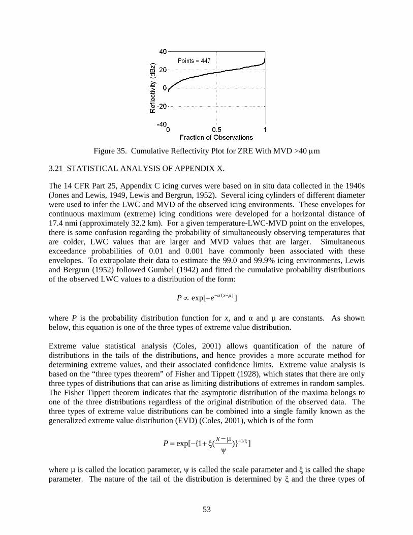
Figure 35. Cumulative Reflectivity Plot for ZRE With MVD >40 μm

3.21 STATISTICAL ANALYSIS OF APPENDIX X.

The 14 CFR Part 25, Appendix C icing curves were based on in situ data collected in the 1940s (Jones and Lewis, 1949, Lewis and Bergrun, 1952). Several icing cylinders of different diameter were used to infer the LWC and MVD of the observed icing environments. These envelopes for continuous maximum (extreme) icing conditions were developed for a horizontal distance of 17.4 nmi (approximately 32.2 km). For a given temperature-LWC-MVD point on the envelopes, there is some confusion regarding the probability of simultaneously observing temperatures that are colder, LWC values that are larger and MVD values that are larger. Simultaneous exceedance probabilities of 0.01 and 0.001 have commonly been associated with these envelopes. To extrapolate their data to estimate the 99.0 and 99.9% icing environments, Lewis and Bergrun (1952) followed Gumbel (1942) and fitted the cumulative probability distributions of the observed LWC values to a distribution of the form:

]exp[ )( μα −−−∝ xeP where P is the probability distribution function for x, and α and µ are constants. As shown below, this equation is one of the three types of extreme value distribution. Extreme value statistical analysis (Coles, 2001) allows quantification of the nature of distributions in the tails of the distributions, and hence provides a more accurate method for determining extreme values, and their associated confidence limits. Extreme value analysis is based on the “three types theorem” of Fisher and Tippett (1928), which states that there are only three types of distributions that can arise as limiting distributions of extremes in random samples. The Fisher Tippett theorem indicates that the asymptotic distribution of the maxima belongs to one of the three distributions regardless of the original distribution of the observed data. The three types of extreme value distributions can be combined into a single family known as the generalized extreme value distribution (EVD) (Coles, 2001), which is of the form

1/ξμexp[ {1 ξ( )}ψ

xP − ]−= − +

where µ is called the location parameter, ψ is called the scale parameter and ξ is called the shape parameter. The nature of the tail of the distribution is determined by ξ and the three types of

53

extreme value distributions are related to whether ξ = 0 (Gumbel family), ξ >0 (Fréchet family) or ξ <0 (Weibull family) as follows:

when ξ = 0 - ∞ < x < ∞ ]exp[ xeP −−=

when ξ > 0 α = 1/ξ 0 < x < ∞ ]exp[ α−−= xP

when ξ < 0 α = -1/ξ - ∞ < x < 0 ])(exp[ αxP −−=

The Gumbel family of distributions has medium-tailed distributions. Distributions, such as the normal, lognormal, exponential and gamma distributions, lie in the domain of convergence of the Gumbel family. This implies that the distribution of the maximum of a sample of size n from any of these distributions will eventually have the Gumbel distribution as n becomes large. The Fréchet family of distributions has tails that are wider, or longer, than the Gumbel family. Distributions that lie in the domain of convergence of the Fréchet family include the Cauchy and the student-t distributions. The Weibull family of distributions has tails that are narrower, or shorter, than the Gumbel family. Distributions in the domain of convergence of the Weibull family include uniform and beta distributions. There are several techniques for estimating the parameters associated with the EVD (Coles, 2001). The technique of threshold selection was used here. This involved sorting the data from the smallest to the largest value, then choosing a threshold value, and finally fitting a generalized Pareto distribution to all of the observations that exceed the threshold value. The distribution of values above a threshold can be approximated by a generalized Pareto distribution (Gencay, et al., 2002). It can be shown that the generalized Pareto distribution is analogous to the EVD with both distributions having a similar form and the same shape parameter (Coles, 2001). When choosing a threshold, care must be taken to balance the number of exceedances of the threshold with the number of data points necessary for a good fit. Choosing a low threshold will allow more data points for the fit but may incorporate data from the centre of the distribution, rather than from only the tail. Choosing a high threshold will better represent the tail however there may be insufficient data points for an adequate fit. Sensitivity studies are required to ensure that the choice of threshold provides results that are reasonable and robust. The in situ aircraft icing data were analysed using the extreme value analysis software described by Gencay, et al. (2002). The method of fitting the data to the EVD and of estimating the shape of the tail of the distribution is discussed in Cober, et al. (2006). A brief summary of the methodology follows. Following Gencay, et al. (2002) the shape of the tail of each SLD distribution was estimated as a function of the threshold (exceedance value) by fitting the data to a generalized Pareto distribution. A threshold value was selected above which the shape factor was observed to be relatively stable. The LWC values greater than the threshold, representing the tail of the distribution, were then fit using a generalized Pareto distribution. The 99% and 99.9% LWC values were determined from the fit with corresponding 95% confidence intervals. Sensitivity studies were done with different threshold values to ensure that the choice of threshold did not significantly influence the results.

54

The number of data points at 30-s resolution for the four SLD subsets ranged from 193 to 1469. To maximize the number of data points used in the analysis, no further subdividing of the SLD subsets (i.e., as a function of temperature or MVD) was undertaken. Table 10 shows, for each SLD subset, the threshold values that were used when fitting the data to a generalized Pareto distribution. Table 10 also shows the maximum observed LWC, the LWC corresponding to the threshold selection, and the shape factor determined for each fit. The standard deviation (σ) for each shape factor is listed in table 10. The shape factors were fairly similar and generally agreed within their standard deviations. The shape factors suggested narrow tailed distributions.

Table 10. Threshold Characteristics for the EVD for Each SLD Environment

SLD Environment

Number of Data Points

Threshold Point

Threshold LWC

(g m-3)

Maximum Observed

LWC (g m-3)

Shape Factor ξ ± σ

ZLE MVD <40 μm 1469 1375 0.39 0.77 -0.04 ±0.10 ZLE MVD >40 μm 335 300 0.20 0.39 -0.28 ±0.14 ZRE MVD <40 μm 193 150 0.17 0.49 -0.14 ±0.11 ZRE MVD >40 μm 447 410 0.19 0.41 -0.09 ±0.14 For each of the four SLD environments, the 99% and 99.9% LWC values, along with their 95% confidence limits, were estimated from the extreme value analysis. These estimates are compared with those obtained from gamma, exponential, and Weibull distributions in figure 36. The exponential distribution always overestimated the extreme values in comparison to the EVD. The gamma distribution values are higher than those from the extreme value distribution, and the two do not agree for ZLE with MVD <40 μm. Conversely, the Weibull distribution generally agreed with the EVD within the 95% confidence limits. The 99.9% LWC values have significant uncertainty, which is related to the limited number of extreme (i.e., above 99%) LWC environments observed. The extreme value analysis was used for the determination of Appendix X. However, given the agreement between the EVD fits and the Weibull distribution fits, if the Weibull-based LWC values had been used, the results would have been similar. The Weibull analysis was not dependent on the selection of a threshold value and might be more easily reproduced by other groups who may wish to compute other percentile values from the database.

55

Figure 36. Comparison of the 99.0% and 99.9% LWC Values for 30-Second Data Obtained From the EVD, Gamma, Exponential, and Weibull Distributions for Each SLD Environment

The numerical values of the EVA 99.0% and 99.9% LWC values for each SLD subset valid for 17.4 nmi are listed in table 11. Note that the maximum LWC values in table 3 are equal to the 99.0% LWC values in table 11. Figures 37-40 compare the 99.0% and 99.9% EVA LWC values to the SLD conditions for 30-second and 300-second data. The EVD 95% confidence limits are also shown in figures 39 and 40 for the 30-second data. There were no observations of SLD environments that had a probability that was lower than the upper 95% confidence limit of the 99.9% LWC value (1-F(x) = 0.001).

Table 11. The 99.0% and 99.9% LWC Values for 17.4 nmi Determined With Extreme Value Analysis

Definition MVD Dmax 99.0% LWC 99.9% LWC ZLE <40 μm 100-500 μm 0.44 g m-3 0.58 g m-3 ZLE >40 μm 100-500 μm 0.27 g m-3 0.31 g m-3 ZRE <40 μm >500 μm 0.31 g m-3 0.37 g m-3 ZRE >40 μm >500 μm 0.26 g m-3 0.33 g m-3

3.22 COMPARISON OF APPENDIX X WITH 14 CFR PART 25 APPENDIX C AND OTHER ICING ENVELOPES.

The 14 CFR Part 25, Appendix C curves were based on in situ data collected in the 1940s (Jones and Lewis 1949, Lewis and Bergrun 1952), and only include MVD values up to 40 μm. Although, Jones and Lewis (1949) suggested that extreme freezing rain conditions could be represented by a droplet MVD of 1000 μm, LWC of 0.15 g m-3, and a horizontal extent >100 km. Newton (1978) described icing accumulation envelopes, which physically represented the sweep out LWC and the potential accumulations of ice on a 3-inch-diameter icing cylinder in g cm-2 h-1. The potential accumulation rate would depend on the collision-collection efficiency of the

56

hydrometeor spectra, which is a function of aircraft speed and droplet size. However, for drops greater than approximately 50 μm in diameter, the collision efficiency would be essentially 1, and there would be no way to distinguish the accumulation associated with 50 μm drops with that from 500 μm or 1000 μm drops. The Appendix X conditions along with the corresponding 99% and 99.9% LWC values will be compared with the potential accumulation envelopes of Newton (1978) and with the maximum LWC envelopes of 14 CFR Part 25, Appendix C in the next section. The Appendix X ZLE and ZRE conditions for horizontal extents of 300-s (30 km) are compared to the 14 CFR Part 25, Appendix C and the potential accumulation envelopes in figures 37 and 38, respectively. The 99% and 99.9% LWC limits computed for Appendix X and given in tables 3 and 11 for 17.4 nmi (32.2 km) horizontal extents are also shown for the MVD <40 μm and MVD >40 μm conditions. The 99% Appendix X LWC limits are shown as solid black lines, while the 99.9% Appendix X LWC limits are shown as dotted black lines. The potential accumulation envelopes for 1, 6, and 12 g cm-2 h-1 are shown as purple lines and labeled with the numbers 1, 6, and 12, respectively. The 14 CFR Part 25, Appendix C curves for 0, -10, and -20 C are shown as blue lines and are labeled as 0, -10, and -20, respectively. The 300-s data are shown by green and red dots representing MVD <40 μm and MVD >40 μm, respectively. Note that the 14 CFR Part 25, Appendix C envelopes and the Appendix X LWC limits are valid for 32.2 km, while the individual data points are valid for 30 km. The comparison is acceptable because the difference in length scales is quite small. Since the Appendix X data are not segregated by temperature and include all observations at temperatures <0 C, it is only valid to compare the Appendix X data and envelopes with the 0oC envelope for 14 CFR Part 25, Appendix C. For the MVD <40 μm conditions, the 14 CFR Part 25, Appendix C envelope for 0 C seems to capture the data extremely well, which suggests that the Appendix X data are consistent with the 14 CFR Part 25, Appendix C data at MVD <40 μm. For MVD >40 μm conditions, the potential accumulation envelope of approximately 10 g cm-2 h-1 bounds the data very well. Newton (1978) suggested that a potential accumulation of 12 g cm-2 h-1 could be interpreted as severe icing. The 99% and 99.9% LWC limits for Appendix X are smaller than the qualitatively named severe icing potential accumulation envelopes. It is interesting to note that a single potential accumulation envelope of 10 g cm-2 h-1 would have captured all but one 300-s Appendix X observations at all MVD values. The potential accumulation envelopes are more physically based than those in 14 CFR Part 25, Appendix C. The consistency of the SLD observations with the potential accumulation envelopes suggests that a maximum potential accumulation envelope could have formed the basis of an alternative SLD environmental characterization. A more detailed comparison of the CFDE I and CFDE III data with these and other icing envelopes was given by Cober, et al. (2001a).

57

Figure 37. Plot of MVD vs LWC for 300-s Averaged Data for ZLE Conditions

Figure 38. Plot of MVD vs LWC for 300-s Averaged Data for ZRE Conditions

58

Because of the limited number of SLD conditions at 300-s or 30 km resolution, it can be difficult to visually reconcile the individual data shown in figures 37 and 38 with the 99% and/or 99.9% LWC envelopes. Figures 39 and 40 show the MVD versus LWC for 30-s (3-km) averaged data for ZLE and ZRE conditions, respectively. The 99% and 99.9% LWC envelopes were computed using the SF in figure 6 and the 99% and 99.9% LWC values for 17.4 nmi from table 11. The 95% confidence limits for the 99% and 99.9% Appendix X LWC values are shown as solid and dotted vertical bars, respectively. Note that the potential accumulation envelopes for 1, 6, and 12 g cm-2 h-1 are shown in figures 39 and 40. However, the 14 CFR Part 25, Appendix C envelopes are not shown because they were not valid at 3 km. The applicability of the 99% envelopes to the data is much clearer to visualize in these figures. It can be observed that approximately 1% of the Appendix X observations exceed the 99% LWC envelopes, which is consistent with the 99% analysis. There are enough data points to have a high degree of confidence in the 99% LWC analysis. This is further demonstrated by the small width of the 95% confidence limits for the 99% LWC analysis. The 99.9% LWC analysis had significantly wider 95% confidence limits, and there were no SLD observations that exceeded the upper confidence limit of the 99.9% LWC envelopes. A potential accumulation envelope of 12 g cm-2 h-1 would bound all of the ZRE observations and 99.5% of the ZLE observations at 3-km resolution.

Figure 39. Plot of MVD vs LWC for 30-s Averaged Data for ZLE Conditions

59

Figure 40. Plot of MVD vs LWC for 30-s Averaged Data for ZRE Conditions

3.23 REPRESENTATIVE COMPARISON OF THE EC/NASA DATA TO OTHER DATA SETS.

It could be argued that the EC/NASA database is biased towards extreme values because the aircraft was deliberately flown into the most severe conditions. To test this hypothesis, a comparison was done between the EC/NASA data set for freezing drizzle and rain and the data sets obtained from surface measurements. The surface measurements were not biased but represent two long term series of data obtained by using a Precipitation Occurrence Sensor System (POSS) (Sheppard, 1990) at St. John’s Newfoundland from 1997 to 2004 and a regular weighing gauge used at 6 stations in Quebec from 1997-2003. The data were provided by private communication from Brian Sheppard of Environment Canada and Barry Myers of Transport Canada. Table 12 shows the percentiles for freezing drizzle and freezing rain based on unbiased surface measurements are very similar to those obtained from the in-flight measurements used to produce Appendix X. The in-flight values were obtained by integrating each individually measured 30-s spectra to obtain rainfall rate. The two freezing drizzle environments were combined into a single category. Similarly, the two freezing rain environments were combined into a single category. Using the Marshall and Palmer (1948) relationship, rainfall rate (mm hr-1) can also be empirically related to LWC (g m-3) through the equation, M=0.072R0.88. So, for the 99% value for measured surface freezing rainfall rate of 4.3 mm hr-1, the LWC mass is 0.26 g m-3, which is quite close to the value being used in Appendix X for freezing rain. This analysis clearly indicates that the 99% values in Appendix X are not overly biased by the sampling strategy used to collect the in-flight data.

60

Table 12. Percentiles of Precipitation Rate for SLD Environments as Obtained From Rain Gauges, POSS, and In-Flight Instruments

50% 75% 95% 99.0%Method Type Precipitation Rate mm/hr In-Flight ZLE 0.03 0.07 0.26 0.60 POSS ZLE ~0.1 ~0.2 0.4 0.65 In-Flight ZRE 0.50 1.1 2.1 3.2 POSS ZRE 0.65 1.2 3.0 7.9 Gauge ZRE 0.67 1.7 3.3 4.3

Determining the actual frequency of occurrence of SLD in the atmosphere is difficult using the in situ data. It is recognized that there are geographic differences and changes with season. For maritime environments, based on all flights conducted during CFDE I, SLD environments that included drops larger than 100 µm in diameter were observed 6.8% of the in-flight time. For continental environments, based on all flights conducted during CFDE III, AIRS, and NASA Pre-AIRS, SLD environments were observed 5.9% of the in-flight time. The percentage of in-flight time with MVD greater than 40 µm (outside of Appendix C) was 3.8% for the maritime clouds and 1.7% for the continental clouds. Similar results using different subsets of the same data were reported by Isaac, et al. (2001a). These percentages should not be used to directly specify the probability of occurrence of SLD because the research flights were targeted at areas where SLD was expected. Consequently, the random probability of encountering a SLD environment should be lower. For example, the frequency of occurrence of freezing precipitation at the ground represents approximately 1% of the time averaged over the winter season for most of Canada with greater values occurring in the Great Lakes area (2%) and in Newfoundland (5%) (Stuart and Isaac, 1999). When all portions of Canada and the United States (including Alaska and Hawaii) are considered, SLD was present in 0.64% of all surface observations made at subfreezing temperatures regardless of time of year (139,196 out of 21,592,596 reports). 3.24 THE LWC VS TWC EXTREMES.

The IPHWG considered the possibility that mixed phase or glaciated clouds might contain TWC extremes that could be greater than the LWC extremes used to produce Appendix X. Appendix X was formed using data obtained in all liquid clouds and in mixed phase clouds with low ice crystal concentrations. Mixed phase clouds with ice crystal concentrations >1 L-1 and glaciated clouds were excluded from the Appendix X analysis following the procedure outlined in Cober, et al. (2001b). Figure 41 shows the cumulative frequency distributions of TWC for liquid, mixed, and glaciated clouds as observed during the same field programs that were used for developing Appendix X. The frequency distributions and extreme values for liquid and mixed-phase conditions are quite similar. The glaciated phase clouds observed tended to have lower TWC values than the mixed and liquid phase clouds. This justifies basing the analysis of data extremes for Appendix X on the liquid and mixed phase clouds with low ice crystal concentrations where the confidence in the quality of the measurements was greatest. This does not suggest that glaciated and mixed

61

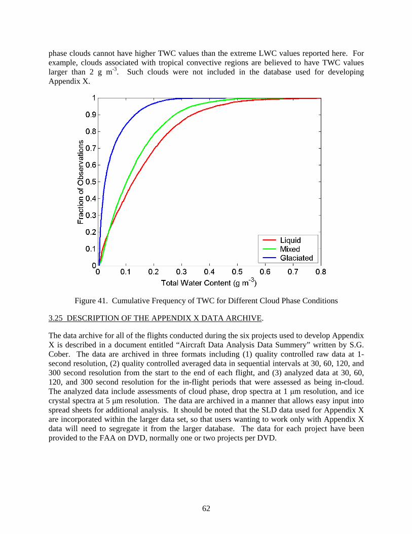
phase clouds cannot have higher TWC values than the extreme LWC values reported here. For example, clouds associated with tropical convective regions are believed to have TWC values larger than 2 g m-3. Such clouds were not included in the database used for developing Appendix X.

Figure 41. Cumulative Frequency of TWC for Different Cloud Phase Conditions

3.25 DESCRIPTION OF THE APPENDIX X DATA ARCHIVE.

The data archive for all of the flights conducted during the six projects used to develop Appendix X is described in a document entitled “Aircraft Data Analysis Data Summery” written by S.G. Cober. The data are archived in three formats including (1) quality controlled raw data at 1-second resolution, (2) quality controlled averaged data in sequential intervals at 30, 60, 120, and 300 second resolution from the start to the end of each flight, and (3) analyzed data at 30, 60, 120, and 300 second resolution for the in-flight periods that were assessed as being in-cloud. The analyzed data include assessments of cloud phase, drop spectra at 1 μm resolution, and ice crystal spectra at 5 μm resolution. The data are archived in a manner that allows easy input into spread sheets for additional analysis. It should be noted that the SLD data used for Appendix X are incorporated within the larger data set, so that users wanting to work only with Appendix X data will need to segregate it from the larger database. The data for each project have been provided to the FAA on DVD, normally one or two projects per DVD.

62

3.26 LIMITATIONS OF THE EC/NASA DATA.

It is important to note that the EC/NASA data were collected during 134 research flights, and that these flights were conducted during 6 field programs and in 3 different geographic locations. CFDE I was conducted in a maritime environment; CFDE III, AIRS, AIRS-NASA, and the NASA-SLD projects were conducted in a continental region around the Great Lakes; and FIRE.ACE was conducted in an Arctic region. Hence, the data may not be representative of all geographic regions or be sufficient for geographical regions such as maritime or Arctic. As an example of geographical variability, Isaac, et al. (2001a) showed that the percentage of the in-flight icing time with drops greater than 50 µm was 73% in the maritime area near CFDE versus 41% in the continental area where CFDE III and AIRS I were conducted. The frequency of occurrence of glaciated clouds was also much higher in the maritime area (33% versus 17%). Although the median measured LWC using 30s values was 0.1 gm-3 for both areas with the average temperature near -5°C, the droplet concentration was much higher in the continental area (120 versus 50 drops per cm-3) and the MVD was much higher in the maritime area (24 versus 17 µm). These droplet concentration and MVD differences between maritime and continental clouds are well known and thought to be due to differences in the properties of the aerosol that form the cloud forming nuclei. Some SLD forming conditions, such as those associated with orographic lift, are not represented in this subset. The data were collected entirely in stratiform winter clouds, hence the data set contains no cases from convective (intermittent maximum) regions. With only 134 research flights, it is likely that the most extreme icing environments existing in nature were not observed. However, considering that the average spectra are quite consistent in shape, it is suggested that for stratiform cloud conditions, the shapes of the characteristic spectra presented here should be applicable for most stratiform cloud conditions. Assuming that the spectra shapes are representative, more extreme icing environments for stratiform cloud conditions could be determined by scaling only the LWC values. 4. FREQUENCY OF SLD CONDITIONS.

4.1 FREQUENCY ESTIMATED USING CIP ALGORITHM.

To estimate the frequency of SLD icing conditions using SLD Potentional (SLDPOT) over North America and Europe, a special version of the CIP algorithm was applied to historical matched surface and sounding data. In all, 14 years of data from the U.S. and Canada and 15 years of data from Europe and Asia were used, resulting in two published studies (Bernstein, et al., 2003 and Bernstein, 2005) and one that is under development (Bernstein, 2009). This chapter summarizes the main results in those studies. Meteorologists at the NCAR developed a multiple data source, hybrid approach to the diagnosis of icing, the CIP. In March 2002, CIP became an official FAA and National Weather Service product. The operational version combines satellite, radar, surface, and lightning observations with numerical model output and pilot reports (PIREP) of icing to create an hourly, three-dimensional diagnosis of the potential for icing and SLD. CIP uses observations to diagnose the locations of clouds and precipitation, and then combines them with numerical model output in a

63

situationally based, fuzzy logic system. The physical structure of the atmosphere is assessed for each vertical column and an icing scenario is identified using a decision tree. Data are treated differently for each scenario, and fuzzy logic membership functions are applied to fields, such as temperature and relative humidity, in an appropriate manner. The algorithm determines icing and SLD potentials for each level in the column. The potential is essentially a confidence or likelihood that such conditions were present. Their presence becomes more likely at the higher thresholds, and the algorithm is more efficient at capturing the actual presence of such conditions while warning for a relatively small volume of airspace in this range. Throughout this section, the threshold of 0.4 will be used. Locations where potentials exceeded 0.4 were considered to have had a good potential for the conditions, while experience indicates that this threshold is fairly efficient in avoiding overwarning or overdiagnosing. Regardless of threshold choice, geographic patterns and vertical distributions in the results were essentially the same. Sensitivity tests indicated that the use of higher thresholds resulted in lower frequencies and shallower layers. A more complete description of CIP, its components and application of fuzzy logic is found in Bernstein, et al. (2005). A special version of CIP was developed that diagnoses icing and SLD potentials in a column using the vertical profile of temperature and moisture from a balloon-borne sounding combined with coincident surface observations. Such an approach can be applied to historical datasets to determine the frequency at which icing and SLD can be expected above a given site as well as across a region, continent, or even the globe. The CIP sounding technique essentially mirrors that of the real-time CIP described in Bernstein, et al. (2005). For this study, the cloud top height and temperature were determined using the moisture profile in the sounding, rather than satellite data, while the occurrence of precipitation and precipitation type were determined solely from surface observations, rather than both surface observations and radar reflectivity. Stricter versions of the relative humidity and cloud top temperature membership functions were applied because the improved quality of moisture data in soundings (compared to numerical weather model forecasts) provided more accurate estimates of cloud locations and cloud top temperatures. Two primary mechanisms are responsible for the formation of nonconvective SLD and are diagnosed by CIP: classical and nonclassical. By determining the mechanism and examining the temperature and moisture profiles as well as the observed precipitation type, the sounding CIP was used to assess the SLD potential. Using this approach, only the potential presence of drops with maximum diameters in excess of ~200 microns is assessed. It is not possible to estimate DSD or MVD. Classical SLD occurs when a layer of T >0°C (warm nose) was located between two layers with T <0°C, freezing or liquid precipitation was observed at the surface, and the CTT (cloud top temperature) was less than -12°C (figure 42 (A)). The relatively cold CTT indicates that an ice process was likely to have been active above the warm nose. Snow fell into the warm nose, melted to form liquid precipitation, which then fell into the lower subfreezing layer to form classical SLD, usually in the form of freezing rain (FZRA). The precipitation typically reached the surface in the form of FZRA, ice pellets (PL), or rain (RA), depending on the strength (depth and temperature) of the warm nose and the temperature and relative humidity within and beneath the lower subfreezing layer.

64

Figure 42. Examples of (A) Classical and (B) Nonclassical SLD

The warm nose is marked in figure 42(A). Temperature and dewpoint profiles are shown in the left-hand panels. Grey shaded areas indicate cloud vertical extent. SLDPOT profiles (gray lines) are given in the right-hand panels, with the SLD layer tops and bases indicated. Figure 42(B) shows nonclassical (collision-coalescence) icing and SLD are identified for three situations: (1) freezing or liquid precipitation was observed when a classical warm nose was present, but CTT was greater than -12°C, indicating a good chance that an all-liquid process was responsible for the precipitation formation; (2) no warm nose was present, only RA and/or DZ were observed at the surface, and CTT was greater than -12°C; and (3) no warm nose was present and freezing precipitation (FZDZ, FZRA, PL) was observed at the surface. CTT was not a factor in case 3, since the precipitation had to have been formed via collision-coalescence. Each sounding was examined for its SLD potential at every level. Frequencies (percent) were calculated by dividing the number of soundings that had SLDPOT ≥0.4 at any level in the sounding by the total number of soundings examined. Figures 43 and 44 show the full-year geographic distribution of SLD icing frequencies for North America and most of Europe, respectively, using an SLDPOT threshold of 0.4. When considering whether SLDPOT exceeded 0.4 at any level in the column, most of North America has SLD frequencies below 3%, while maximum frequencies are on the order of 5% to 8%. While the frequencies may seem large, recall that they are calculated using a low-to-moderate SLDPOT threshold (0.4) and that they indicate the frequency of occurrence of conditions that are conducive to SLD at any altitude (up to ~10 km [30,000 ft mean sea level (MSL)]), anywhere within 100 km of the sounding site. This represents a 314,000 km3 volume of airspace above a given station. Likewise, values for individual 1-km (~3000 ft) thick altitude ranges represent 31,400 km3 volume of airspace above a given station. Thus, the percentages do not represent point or instantaneous frequencies of SLD (i.e., that SLD would be encountered during 5% to 8% of the time during random flight within the area of peak SLD frequencies). Frequencies of aircraft SLD encounters are expected to be much lower. Note that absolute frequencies depend heavily on threshold choice. The choice of the 0.4 SLDPOT threshold is based upon the experience of the algorithm developers,

65

which indicates a reasonably good confidence that SLD was present and over warning is mitigated.

% of soundings with SLDPOT ≥0.4

Figure 43. Inferred Full-Year Column SLD Icing Frequencies for Canada and the Continental United States (Values are the percentage of all soundings tested at each location that had

SLDPOT ≥0.4 at some level.)

66

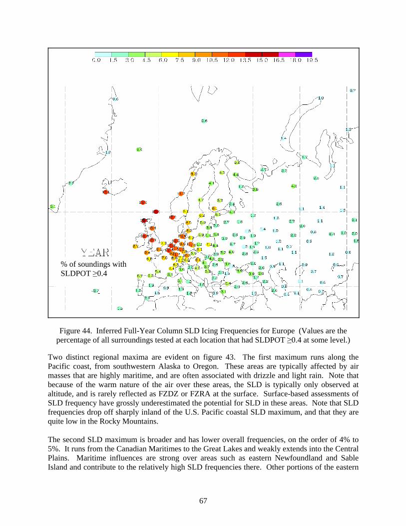
% of soundings with SLDPOT ≥0.4

Figure 44. Inferred Full-Year Column SLD Icing Frequencies for Europe (Values are the percentage of all surroundings tested at each location that had SLDPOT ≥0.4 at some level.)

Two distinct regional maxima are evident on figure 43. The first maximum runs along the Pacific coast, from southwestern Alaska to Oregon. These areas are typically affected by air masses that are highly maritime, and are often associated with drizzle and light rain. Note that because of the warm nature of the air over these areas, the SLD is typically only observed at altitude, and is rarely reflected as FZDZ or FZRA at the surface. Surface-based assessments of SLD frequency have grossly underestimated the potential for SLD in these areas. Note that SLD frequencies drop off sharply inland of the U.S. Pacific coastal SLD maximum, and that they are quite low in the Rocky Mountains. The second SLD maximum is broader and has lower overall frequencies, on the order of 4% to 5%. It runs from the Canadian Maritimes to the Great Lakes and weakly extends into the Central Plains. Maritime influences are strong over areas such as eastern Newfoundland and Sable Island and contribute to the relatively high SLD frequencies there. Other portions of the eastern

67

maximum, such as the Great Lakes and Central Plains have relatively little maritime influence. In these areas with strong continental influence, the SLD is typically associated with the northern side of storm systems as they track from northern Texas to the Mid-Atlantic or Northeastern coastal regions. Past surface- and aircraft-based studies have shown that FZRA and FZDZ are commonly found on the cold side (typically to the north of) warm fronts and stationary fronts, and some is found in the wake of strong cold fronts. The strongest SLD minima are found over the Intermountain West, southern California, and along the Gulf Coast. Most portions of Europe and surrounding areas had SLD frequencies that were <5%. The primary SLD maxima were found over the United Kingdom (UK), western Scandinavia, and around northern Germany, with frequencies between 8% and 15%. Peak values were found in a swath from the Northern UK and western Scandinavia to Iceland. These areas are strongly influenced by maritime air masses. The second maximum was over northern Germany and the Benelux region, which has influence from the North Sea, but also has a good frequency of frontal and storm activity. Minimum frequencies occurred over southern Europe, especially near the Mediterranean Sea, as well as large portions of Russia. Overall, Europe appeared to have SLD somewhat more frequently than North America. However, it is very important to note that the vertical resolution of sounding observations over Europe (and Asia, see figure 45) were somewhat poorer than those for North America. This decreases confidence in the results over these continents and may have skewed them upward. While the confidence in the absolute frequencies is not as high, the patterns are still quite meaningful. Confidence in the absolute frequencies over North America is higher thanks to the quality of the sounding data, in conjunction with the abundance of operational and research aircraft observations, as well as surface observations in most of the SLD-prone areas. These observations corroborate many of the findings of the inferred SLD climatology. Similar to Europe, most portions of Asia for which data was available had SLD frequencies that were <5%. Overall, SLD was primarily found in a swath from southeastern China to Japan, and included South Korea and Taiwan. Peak frequencies were on the order of 7%-8% and were found over southwestern Japan and inland portions of southeastern China. Little information was available for the region stretching from Vietnam to Iran, including India. SLD frequencies were relatively low over most of Russia, perhaps due to issues with surface reporting of precipitation type. SLD frequencies were also quite low over equatorial regions, but this may be the result of limitations in the methodology used in this study. The method only indicates SLD aloft when liquid precipitation falls to the ground from subfreezing clouds that meet certain criteria. This combination of conditions may be difficult to achieve for tropical clouds, since the freezing level is often quite high. Over all three continents, SLD maxima moved latitudinally with season. In general, maxima were found at northern latitudes, including along the Arctic Coast during the summer months and moved southward to the reach the middle and even southern areas (to near 30oN latitude) during the winter. During the spring, they moved northward again. Though relatively low overall SLD frequencies were found along the Arctic Coast, this area had peak frequencies on the order of 5% during July and August.

68

% of sounding with SLDPOT ≥ 0.4

Figure 45. Inferred Full-Year Column SLD Icing Frequencies for Asia (Values are the percentage of all surroundings tested at each location that had SLDPOT ≥0.4 at some level.)

The overall inferred chance of encountering SLD icing conditions, as defined at the beginning of this section, was on the order of 1% to 2% given flight through any given1-km deep altitude band (e.g., 2 to 3 km or ~6000 to 9000 ft MSL within a 100 km radius. This value was calculated by summing the number of times that SLD potential exceeded 0.4 in each 1-km (3000 ft) altitude band for all sites and dividing that number by the total number of samples available for this study. Recall that the 1%-2% value represents the percentage of time the SLD is expected to exist somewhere within this 31,400 km3 of airspace, and this value does not represent an expected chance for encountering SLD during flight. It is important to note that the methods used here will only capture SLD events that are reflected at the surface, matched with certain structures aloft. This will only capture a subset of all SLD icing events, as SLD occurs aloft in cases where freezing or liquid precipitation is not observed at the surface. Verification of the SLD icing algorithm has been rather limited, but a comparison between winter 1997-98 NASA GRC Twin Otter SLD observations and a similar version of the full CIP SLD icing algorithm (using surface observations in combination with satellite and radar data, as well as

69

numerical model output) showed that CIP captured almost every SLD icing event. Larger, more recent data sets are available from NASA and EC, but such analysis has not been completed to date. However, a study using a rather limited database of PIREPs of icing that specifically mention “FZDZ” or “FZRA” in the comments found that the CIP SLD algorithm captured ~32%. Reality is likely to be somewhere in between. Neither of these comparisons were done using the sounding CIP, but the algorithms are reasonably similar. Both results are based on low thresholds of SLD potential (e.g., 0.02 on a scale of 0.0 to 1.0). 4.2 FREQUENCY ESTIMATED USING OTHER SOURCES OF DATA.

The Canadian in situ icing database (Isaac, et al., 2001a) shows that SLD conditions in supercooled cloud (-40°C<T <0°C, and ice particle concentration <1 litre-1) with maximum drop size greater than 50 µm represent an average of 13% of in-flight time in the maritime clouds (CFDE I) and 8.6% of the time in continental clouds (CFDE III and AIRS I). The percentage of in-flight time with MVD >40 µm (outside of 14 CFR Appendix C) was 3.6% for the maritime clouds and 1.3% for the continental clouds. These percentages cannot be used to represent the probability of occurrence of SLD because flights were directed into areas with icing that were expected to contain SLD. Consequently, the true probability of occurrence of SLD would be lower. For example, the frequency of occurrence of freezing precipitation at the ground represents approximately 1% of the time averaged over the winter season for most of Canada with greater values occurring in the Great Lakes area (2%) and in Newfoundland (5%). (Stuart and Isaac, 1999). A similar study to that of Stuart and Isaac (1999) was undertaken for this report, using surface observations for all of Canada and the United States for the years 1977 to 1990. SLD was considered to have been present if FZDZ or FZRA was observed at the surface. As described in section 3.23, when all times of year are considered, SLD was present in 0.64% of all surface observations made at subfreezing temperatures. Newfoundland typically had the highest percentage values for SLD, with values on the order of 2% to 4% at T<0°C (3.7% at St. John’s). Values around the Great Lakes were significantly lower and on the order of 0.50% to 1.50%. Interestingly, the greatest SLD percentages for times with T<0°C tended to occur over Texas and Louisiana (3%-9%), where overall SLD frequencies were quite low (typically 0.1% to 0.3%). While subfreezing surface temperatures in this region are relatively unusual, they are often associated with the presence of shallow, moist, surface-based cold air masses that are overrun by relatively warm air. Depending on the temperature and moisture content of the air within and above the warm layer, FZDZ or FZRA can result. Data from Mt. Washington, New Hampshire, U.S. showed SLD in 0.9% of all observations and 1.6% of all subfreezing observations. Monthly values show peak SLD frequencies (regardless of temperature) in the fall and spring (maxima of 2.1% and 1.8% in November and April, respectively), with a relative minimum in midwinter (0.4% in January), very little during June and September, and no SLD during July and August. This pattern and the overall frequencies compare well to those calculated at Mt. Washington’s altitude (~1913m; 6273ft MSL) above nearby sounding sites Portland, Maine; Caribou, Maine; and Albany, New York U.S.). Frequencies at those sites were on the order of 2%-5% during the peak months in fall and winter, decreased somewhat in mid-winter (1%-3%), were very low in June and September (0.1%-0.2%) and zero during July and August. Of course, the sounding-based values are representative of

70

large slabs of airspace, as described above, so they should be quite high compared to those from a single-point measurement in the free atmosphere. However, the observatory at Mt. Washington does not represent such a point because its weather is strongly affected by the lift associated with the mountain itself. Such lift is expected to locally enhance the production of supercooled liquid water, causing anomalously high SLD frequencies at this location compared to a point in the free atmosphere, unaffected by the local terrain. Determining the actual occurrence of SLD in the atmosphere is difficult using the data sets available. It is recognized that there are large geographical differences and changes with season. However, to a first approximation, the probability of occurrence of SLD for any particular location in North America, representing the altitude ranges between 0 and 15,000 ft (5km), which aircraft normally encounter upon takeoff and landing, is typically 0.5% to 5% over a winter season for a large portion of the continent. 5. BIBLIOGRAPHY.

Ashenden, R. and J.D. Marwitz, 1998, “Characterizing the Supercooled Large Droplet Environment With Corresponding Turboprop Aircraft Response,” Journal of Aircraft, Vol. 35, pp. 912-920. Baumgardner, D., and A. Rodi, 1989, “Laboratory and Wind Tunnel Evaluations of the Rosemount Icing Detector,” Journal of Atmospheric and Oceanic Technology, Vol. 6, pp. 971-979. Baumgardner, D., W. Strapp, and J.E. Dye, 1985, “Evaluation of the Forward Scattering Spectrometer Probe. Part II: Corrections for Coincidence and Dead Time Losses,” Journal of Atmospheric and Oceanic Technology, Vol. 2, pp. 626-632. Bernstein, B.C., 2005, “An Inferred European Climatology of Icing Conditions, Including Supercooled Large Droplets,” FAA report DOT/FAA/AR-05/24. Bernstein, B.C., F. McDonough, and R. Bullock, 2003, “An Inferred Climatology of Supercooled Large Droplet Icing Conditions for North America,” 39th Aeropsace Sciences Meeting and Exhibit, 6-10 January, American Institute of Aeronautics and Astronautics, Washington, DC. Also presented at the FAA International Icing Conference, Chicago. Bernstein, B.C. and C. LeBot, 2009, “An Inferred Climatology of Icing Conditions Aloft, Including Supercooled Large Drops. Part II: Europe, Asia, and the Globe,” Accepted to the Journal of Applied Meterology and Climatology. Bernstein, B.C., F. McDonough, M.K. Politovich, B.G. Brown, T.P. Ratvasky, D.R. Miller, C.A. Wolff, and G. Cunning, 2005, “Current Icing Potential (CIP): Algorithm Description and Comparison with Aircraft Observations,” Journal of Applied Meteorology, Vol. 44, pp. 969-986. Bernstein, B.C., C.A. Wolff, and F. McDonough, “An Inferred Climatology of Icing Conditions Aloft, Including Supercooled Large Drops. Part I: Canada and the Continental United States,” Journal of Applied Meterology and Climatology, Vol. 46, No. 11, 2007, pp. 1857-1878.

71

Biter, C.J., J.E. Dye, D. Huffman, and W.D. King, 1987, “The Drop-Size Response of the CSIRO Liquid Water Probe,” Journal of Atmospheric and Oceanic Technology, Vol. 4, pp. 359-367. Byers, H.R., 1944, General Meteorology, Mcgraw-Hill Book Co., New York. Changon, S.A., et al., 1991, “Illinois Precipitation Research: A Focus on Cloud and Precipitation Modification,” Bulletin American Meteorological Society, pp. 587. Cober, S.G. and G.A. Isaac, 2006, “Estimating Maximum Aircraft Icing Environments Using a Large Data Base of In Situ Observations,” AIAA 44th Aerospace Sciences Meeting and Exhibit, Reno, Nevada, 9-12 January 2006, Paper No. AIAA 2006-0266. Cober, S.G., G.A. Isaac, and J.W. Strapp, 1995, “Aircraft Icing Measurements in East Coast Winter Storms,” Journal of Applied Meteorology, Vol. 34, pp. 88-100. Cober, S.G., J.W. Strapp, and G.A. Isaac, 1996, “An Example of Supercooled Drizzle Drops Formed Through a Collision-Coalescence Process,” Journal of Applied Meteorology, Vol. 35, pp. 2250-2260. Cober, S.G., G.A. Isaac, and J.W. Strapp, 2001a, “Characterizations of Aircraft Icing Environments That Include Supercooled Large Drops,” Journal of Applied Meteorology, Vol. 40, pp. 1984-2002. Cober, S.G., G.A. Isaac, A.V. Korolev, and J.W. Strapp, 2001b, “Assessing Cloud-Phase Conditions,” Journal of Applied Meteorology, Vol. 40, pp. 1967-1983. Cober, S.G., G.A. Isaac, and A.V. Korolev, 2001c, “Assessing the Rosemount Icing Detector With In Situ Measurements,” Journal of Atmospheric and Oceanic Technology, Vol. 18, pp. 515-528. Cober, S.G., T.P. Ratvasky, and G.A. Isaac, 2002, “Assessment of Aircraft Icing Conditions Observed During AIRS,” AIAA 40th Aerospace Sciences Meeting and Exhibit, Reno, Nevada, 14-17 January 2002, Paper No. AIAA 2002-0674. Cober, S.G., and G.A. Isaac, 2002, “Aircraft Environments Observed in Mixed-Phase Clouds,” AIAA 40th Aerospace Sci. Meeting and Exhibit, Reno, Nevada, 14-17 January 2002, Paper No. AIAA 2002-0675. Cober, S.G., G.A. Isaac, A.D. Shah, and R. Jeck, 2003, “Defining Characteristic Cloud Drop Spectra From In Situ Measurements,” AIAA 41st Aerospace Sciences Meeting and Exhibit, Reno, Nevada, 6-10 January 2003, Paper No. AIAA 2003-0561. Coles, S., 2001, An Introduction to Statistical Modeling of Extreme Values, Springer. Cooper, W.A., W.R. Sand, M.K. Politovich, and D.L. Veal, 1984, “Effects of Icing on Performance of a Research Aircraft,” Journal of Aircraft, Vol. 21, pp. 708-715.

72

Curry, J.A., P.V. Hobbs, M.D. King, D.A. Randall, P. Minnis, G.A. Isaac, J.O. Pinto, T. Uttal, A. Bucholtz, D.G. Cripe, H. Gerber, C.W. Fairall, T.J. Garrett, J. Hudson, J.M. Intrieri, C. Jakob, T. Jensen, P. Lawson, D. Marcotte, L. Nguyen, P. Pilewskie, A. Rangno, D. Rogers, K.B. Strawbridge, F.P.J. Valero, A.G. Williams, and D. Wylie, 2000, “FIRE Arctic Clouds Experiment,” Bulletin of the American Meteorological Society, Vol. 81, pp. 5-29. Drummond, A.M. and J.I. MacPherson, 1985, “Aircraft Flow Effects on Cloud Drop Images and Concentration Measured by the NAE Twin Otter,” Journal of Atmopheric and Oceanic Technology, Vol. 2, pp. 633-643. Federal Aviation Administration, 1999, U.S. Code of Federal Regulations, Title 14 (Aeronautics and Space), Part 25 (Airworthiness Standard: Transport Category Airplanes), Appendix C, Office of the Federal Register, National Archives and Records Administration, U.S. Government Printing Office, Washington, DC, pp. 478. FAA, 1997, “FAA Inflight Aircraft Icing Plan,” Federal Aviation Administration, Washington, DC 20591. Fisher, R.A. and L.H.C. Tippett, 1928, “Limiting Forms of the Frequency Distribution of the Largest or Smallest Members of a Sample,” Proceedings of the Cambridge Philosophical Society, Vol. 24, pp. 180-190. Fuchs, W. and K.-P. Schickel, 1995, “Aircraft Icing in Visual Meteorological Conditions Below Stratus Clouds,” Atmospheric Research, Vol. 36, pp. 339-345. Gardiner, B.A. and J. Hallett, 1985, “Degradation of In-Cloud Forward Scattering Spectrometer Probe Measurements in the Presence of Ice Particles,” Journal of Atmospheric and Oceanic Technology, Vol. 2, pp. 171-180. Gencay, R., F. Selcuk, and A. Ulugulyagci, 2002, “EVIM: A Software Package for Extreme Value Analysis in MATLAB,” Studies in Nonlinear Dynamics and Econometrics, Vol. 5, pp. 213-239. Gultepe, I., G.A. Isaac, and S.G. Cober, 2002, “Cloud Microphysical Characteristics Versus Temperature for Three Canadian Field Projects,” Annales Geophysicae, Vol. 20, pp. 1891-1898. Gultepe, I. and G.A. Isaac, 2004, “Aircraft Observations of Cloud Droplet Number Concentration: Implications for Climate Studies,” Quarterly Journal of the Royal Meteorological Society, Vol. 130, pp. 2377-2390. Gumbel, E.J., 1942, “On the Frequency Distribution if Extreme Values in Meteorological Data,” Bulletin of American Meteorology Society, Vol. 23, pp. 95-105. Hallett, J. and G.A. Isaac, 2002, “Aircraft Icing in Glaciated and Mixed Phase Clouds,” AIAA 40th Aerospace Sciences Meeting and Exhibit, 14-17 January 2002, Reno, Nevada, Paper No. AIAA 2002-0677.

73

Heymsfield, A.J. and J.L. Parrish, 1978, “A Computational Technique for Increasing the Effective Sampling Volume of the PMS Two-Dimensional Particle Size Spectrometer,” Journal of Applied Meteorology, Vol. 17, pp. 1566-1572. Isaac, G.A. and R.S. Schemenauer, 1979, “Large Particles in Supercooled Regions of Northern Canadian Cumulus Clouds,” Journal of Applied Meteorology, Vol. 18, pp. 1056-1065. Isaac, G.A., S.G. Cober, J.W. Strapp, A.V. Korolev, A. Tremblay, and D.L. Marcotte, 2001a, “Recent Canadian Research on Aircraft In-Flight Icing,” Canadian Aeronautics and Space Journal, Vol. 47, pp. 213-221. Isaac, G.A., S.G. Cober, J.W. Strapp, D. Hudak, T.P. Ratvasky, D.L. Marcotte, and F. Fabry, 2001b, “Preliminary Results From the Alliance Icing Research Study (AIRS),” AIAA 39th Aerospace Sciences Meeting and Exhibit, Reno, Nevada, Paper No. AIAA 2001-0393. Isaac, G.A., S.G. Cober, A.V. Korolev, J.W. Strapp, A. Tremblay, and D.L. Marcotte, 1999, “Canadian Freezing Drizzle Experiment,” AIAA 37th Aerospace Sciences Meeting and Exhibit, Reno, Nevada. Isaac, G.A., S.G. Cober, I. Gultepe, A.V. Korolev, F.S. Boudala, and M.E. Bailey, 2002, “Particle Spectra in Stratiform Winter Clouds,” Proceedings of the 11th AMS Conference Cloud Physics, Ogden, Utah. Jeck, R.K., 1983, “A New Data Base of Supercooled Cloud Variables for Altitudes up to 10,000 Feet AGL and the Implications for Low Altitude Aircraft Icing,” FAA Report DOT/FAA/CT-83/21. Jeck, R.K., 1996, “Representative Values of Icing-Related Variables Aloft in Freezing Rain and Freezing Drizzle,” FAA Report DOT/FAA/AR-TN95/119. Jeck, R.K., 2002, “Icing Design Envelopes (14 CFR Parts 25 And 29, Appendix C) Converted to a Distance-Based Format,” FAA Report DOT/FAA/AR-00/30. Jeck, R.K., [FAA Master SLD Database: Description and Analyses] to be published in 2009. Johl, G., et al., 2000, “Investigation Into the Possibility of Retro-Fitting Improved Tailplane Ice Protection on Turboprop Aircraft,” SAE Paper No. 2000-01-2113, Advances in Aviation Safety Conference and Exposition, April 2000, Society of Automotive Engineers. Jones, A.R. and W. Lewis, 1949, “Recommended Values of Meteorological Factors to be Considered in the Design of Aircraft Ice-Prevention Equipment,” NACA TN-1855. Joe, P. and R. List, 1987, “Testing and Performance of Two-Dimensional Optical Array Spectrometers With Greyscale,” Journal of Atmospheric and Oceanic Technology, Vol. 4, pp. 139-150.

74

King, W.D., 1986, “Air Flow Around PMS Canisters,” Journal of Atmospheric and Oceanic Technology, Vol. 3, pp. 197-198. King, W.D., D.A. Parkin, and R.J. Handsworth, 1978, “A Hot Wire Liquid Water Device Having Fully Calculable Response Characteristics,” Journal of Applied Meteorology, Vol. 17, pp. 1809-1813. King, W.D., J.E. Dye, J.W. Strapp, D. Baumgardner, and D. Huffman, 1985, “Icing Wind Tunnel Tests on the CSIRO Liquid Water Probe,” Journal of Atmospheric and Oceanic Technology, Vol. 2, pp. 340-352. Korolev, A.V., J.W. Strapp, G.A. Isaac, and A.N. Nevzorov, 1998a, “The Nevzorov Airborne Hot-Wire LWC-TWC Probe: Principles of Operation and Performance Characteristics,” Journal of Atmospheric and Oceanic Technology, Vol. 15, pp. 1495-1510. Korolev, A.V., J.W. Strapp, and G.A. Isaac, 1998b, “Evaluation of the Accuracy of PMS Optical Array Probes,” Journal of Atmospheric and Oceanic Technology, Vol. 15, pp. 708-720. Lawson, R.P. and W.A. Cooper, 1990, “Performance of Some Airborne Thermometers in Clouds,” Journal of Atmospheric and Oceanic Technology, Vol. 7, pp. 480-494. Lewis, W., 1951, “Meteorological Aspects of Aircraft Icing. Compendium of Meteorology,” American Meteorological Society, T.F. Malone, ed., Waverly Press Inc., pp. 1197-1203. Lewis, W. and N.R. Bergrun, 1952, “A Probability Analysis of the Meteorological Factors Conducive to Aircraft Icing in the United States,” NACA Technical Note No. 2738, Washington, DC. Lewis, W., 1969, “Review of Icing Criteria,” in Aircraft Ice Protection, FAA Symposium on April 28-30, 1969, Federal Aviation Administration, Washington, DC 20591. Ludlam, F.H., 1951, “The Heat Economy of a Rimed Cylinder,” Quarterly Journal of the Royal Meteorological Society, Vol. 77, pp. 663-666. McKay, G.A. and H.A. Thompson, 1969, “Estimating the Hazard of Ice Accretion in Canada From Climatological Data,” Journal of Applied Meteorology, Vol. 8, pp. 927-935. Marshall, J.S., W. McK. Palmer, 1948, “The Distribution of Raindrops With Size,” Journal of the Atmospheric Sciences, Vol. 5, pp. 165-166. Marwitz, J., M. Politovich, B. Bernstein, F. Ralph, P. Neiman, R. Ashenden, and J. Bresch, 1996, “Meteorological Conditions Associated With the ATR72 Aircraft Accident Near Roselawn, Indiana on 31 October 1994,” Bulletin of the American Meteorological Society, Vol. 78, pp. 41-52.

75

76

Masters, C.O., 1983, “A New Characterization of Supercooled Clouds Below 10,000 Feet AGL,” FAA report DOT/FAA/CT-83/22. Mason, B.J. and B.P. Howorth, 1952, “Some Characteristics of Stratiform Clouds Over North Ireland in Relation to Their Precipitation,” Quarterly Journal of the Royal Meteorological Society, Vol. 78, pp. 226-230. Mazin, I.P., A.V. Korolev, A. Heymsfield, G.A. Isaac, and S.G. Cober, 2001, “Thermodynamics of Icing Cylinder for Measurements of Liquid Water Content in Supercooled Clouds,” Journal of Atmospheric and Oceanic Technology, Vol. 18, pp. 543-558. Miller, D., T. Ratvasky, B. Bernstein, F. McDonough, and J.W. Strapp, 1998, “NASA/FAA/NCAR Supercooled Large Droplet Icing Flight Research: Summary of Winter 96-97 Flight Operations,” AIAA 36th Aerospace Sciences Meeting and Exhibit, Reno, Nevada, 12-15 January 1998, Paper No. AIAA 98-0577. Miller, I. and J.E. Freund, 1965, Probability and Statistics for Engineers, Prentice-Hall, Inc., Englewood Cliffs, New Jersey. NCDC, 1998, “International Surface Weather Observations (1982-1997),” A 5-volume Data Set Released on Compact Discs by the National Climatic Data Center (NCDC), Asheville, North Carolina. (see http://www.ncdc.noaa.gov/onlinestore.html). Newton, D.W., 1978, “An Integrated Approach to the Problem of Aircraft Icing,” Journal of Aircraft, Vol. 15, pp. 374-380. NTSB, 1996, “Aircraft Accident Report, ATR Model 72-212, Roselawn, Indiana, October 31, 1994,” NTSB/AAR-96/01, National Transportation Safety Board. Pobanz, B.M., J.D. Marwitz, and M.K. Politovich, 1994, “Conditions Associated With Large-Drop Regions,” Journal of Applied Meteorology, Vol. 33, pp. 1366-1372. Politovich, M.K., 1989, “Aircraft Icing Caused by Large Supercooled Droplets,” Journal of Applied Meteorology, Vol. 28, pp. 856-868. Politovich, M.K., 1996, “Response of a Research Aircraft to Icing and Evaluation of Severity Indices,” Journal of Aircraft, Vol. 33, pp. 291-297. Rasmussen, R., M. Politovich, J. Marwitz, W. Sand, J. McGinley, J. Smart, R. Pielke, S. Rutledge, D. Wesley, G. Stossmeister, B. Bernstein, K. Elmore, N. Powell, E. Westwater, B.B. Stankov, and D. Burrows, 1992, “Winter Icing and Storms Project (WISP),” Bulletin of the American Meteorological Society, Vol. 73, pp. 951-974. Rauber, R.M. and M.F. Heggli, 1988, “The Influence of Cloud Droplets on the Measurement of Ice Particle Concentrations With a Particle Measuring System’s 2DC Optical Array Probe,” Journal of Atmospheric and Oceanic Technology, Vol. 5, pp. 123-128.

Riley, J.T. (Ed.), 1996, “Proceedings of the FAA International Conference on Aircraft Inflight Icing, Volume 1,” FAA report DOT/FAA/AR-96/81,1. Sand, W.R., W.A. Cooper, M.K. Politovich, and D.L. Veal, 1984, “Icing Conditions Encountered by a Research Aircraft,” Journal of Climate Applied Meteorology, Vol. 23, pp. 1427-1440. Shah, A.D., M.W. Patnoe, and E.L. Berg, 2000, “Engineering Analysis of the Atmospheric Icing Environment Including Large Droplet Conditions,” Society of Automotive Engineers, SAE paper 2000-01-2115. Sheppard, B.E., 1990, “The Measurement of Raindrop Size Distributions Using a Small Doppler Radar,” Journal of Atmospheric and Oceanic Technology, Vol. 7, pp. 255-268. Strapp, J.W., F. Albers, A. Reuter, A.V. Korolev, W. Maixner, E. Rashke, and Z. Vukovic, 2001, “Laboratory Measurements of the Response of a PMS OAP-2DC Probe,” Journal of Atmospheric and Oceanic Technology, Vol. 18, pp. 1150-1170. Strapp, J.W., J. Oldenburg, R. Ide, L. Lilie, S. Bacic, Z. Vukovic, M. Oleskiw, D. Miller, E. Emery, and G. Leone, 2003, “Wind Tunnel Measurements of the Response of Hot-Wire Liquid Water Content Instruments to Large Droplets,” Journal of Atmospheric and Oceanic Technology, Vol. 20, pp. 791-806. Stuart, R.A. and G.A. Isaac, 1999, “Freezing Precipitation in Canada,” Atmosphere Ocean, Vol. 37-1, pp. 87-102. Wright, W.B., 1999, “User Manual for the NASA Glenn Ice Accretion Code LEWICE Version 2.0,” Technical Report NASA/CR-1999-209409. Yau, M.K. and R.R. Rogers, 1989, A Short Course in Cloud Physics, Butterworth-Heinemann, Woburn, Massachusetts.

77/78