Page #1

Don’t say “CAN’T do it”, Say “Gantt it”!

The irony of organizing microprocessors with a big business tool

Do you have a powerful processor with the capability of issuing

many instructions in parallel?

Are you having big problems coding to get the maximum throughput?

Then a big business tool can possible come to your rescue.

Mike Smith and James Miller In this article, Mike and James demonstrate how to use the big business tool Microsoft Project as a nano-second scheduling tool for microprocessors. Published Circuit Cellar magazine, Vol. 184, pp 26 - 35, November 2005.

Contact person M. Smith Electrical and Computer Engineering,

University of Calgary, Calgary, Alberta, Canada T2N1N4

Email: smithmr@ucalgary.ca

Phone (+1) 403-220-6142

Word count 7312 words

Page #2

Don’t say ‘I “CAN’T” do it’, say ‘I can “Gantt” it’! Organizing microprocessors with a big business tool

Sometime after midnight we had a problem working out the best way to optimize the performance of a finite impulse response filter, FIR, on an Analog Devices ADSP-TS201 processor. The TigerSHARC is one fancy, very long instruction word (VLIW) processor with multiple data paths, multiple ALUs and register banks of registers together with CLUs (communication logic units) capable of handling specialized instructions for GPS (global positioning systems) and telecommunications (CDMA) issues via complex arithmetic. We don’t mean complex in the sense of “complicated” and hard to use; we mean specific processor instructions of the form a + jb, where 1j = − ). The way we wanted to use the FIR was special and just was not being optimized “the right way” by the compiler that came with the VisualDSP development environment. However proving our new instruction schedule was both “better” and correct was difficult; especially as we were so tired at that point in night. Browsing through the web did not offer all quick solutions for quick, reliable visualization of possible parallelism instructions on VLIW processors. However, in a moment of lapsed concentration (tiredness induced hallucination), a most unexpected partner was suggested as providing all the answers. “Who are you going to call” when you want a quick visual way of comparing a program across various processor architectures? “Who are you going to call” when you want a way to squeeze the last cycle out of some very parallel code; code that is highly optimized for a specific DSP processor? “Who are you going to call” when you are in the situation where you must move that code to a higher performance processor with a more complicated and convolved instruction and memory pipeline; and you lie awake wondering what will “really” happen to the performance of your code? The answer is more than a little ironic as we found a way of having a big business task scheduling tool -- Microsoft Project -- solve little problems involving nano-second time intervals! In this article we will start by giving a brief example of how Microsoft Project is used by a STL (standard technically literate) person to provide an overview of normal Project terminology. We then need to make the transition from standard Project use (involving tasks over weeks and months) to parallel-processor Project (involving nano-second time periods). The transition is demonstrated by using Project to make a comparison of the performance of a finite impulse response, FIR, filter algorithm on an older Motorola 68K style of processor and the TigerSHARC processor. The extremes between processors could not be more pronounced: the TigerSHARC is a VLIW processor, especially designed for high speed parallel operations, while the 68K, a CISC processor circa 1971, has one data path and 8 data registers. Once we’ve shown you how to use Microsoft Project for basic microprocessor scheduling, we will tackle the more complex issues of loop-unrolling and parallel instruction reordering. How is Project normally used? Before describing how to use the “Microsoft Project” Parallel Instruction Visualization (PIV) tool, a little about Project’s standard uses. This is a “big” business tool designed for scheduling and tracking the progress of large scale projects involving many people (resources) working on multiple interacting tasks. In this article, the first use of any proper Project keyword or terminology will be written in bold-type. The following example demonstrates the way Project is normally used. We have been recently been asked by the Calgary “Deaf and Hard of Hearing” Society (DHH Society) to improve the performance of their “magnetic induction loops” for use at 10 audio stages of a local outdoor folk concert. Audio signals from the performers are sent to an amplifier which produces a current through about 100’ of thin wire buried in the ground (about 10 ohms). This current sets up a local magnetic field which varies with the audio signal. This magnetic field is picked by the ‘T-coil’ in a hearing aid, enabling the DHH person to hear the folk concert without reverberation and other distortion problems the normal hearing person experiences at an outdoor concert. To move this project through to completion, we will need to organize people to design, develop and test digital signal processing algorithms, bury and recover the loop cable at the folk concert site, determine the frequency characteristics of the magnetic loops and the amplifiers, move digging and other equipment to the site; all the time

Page #3

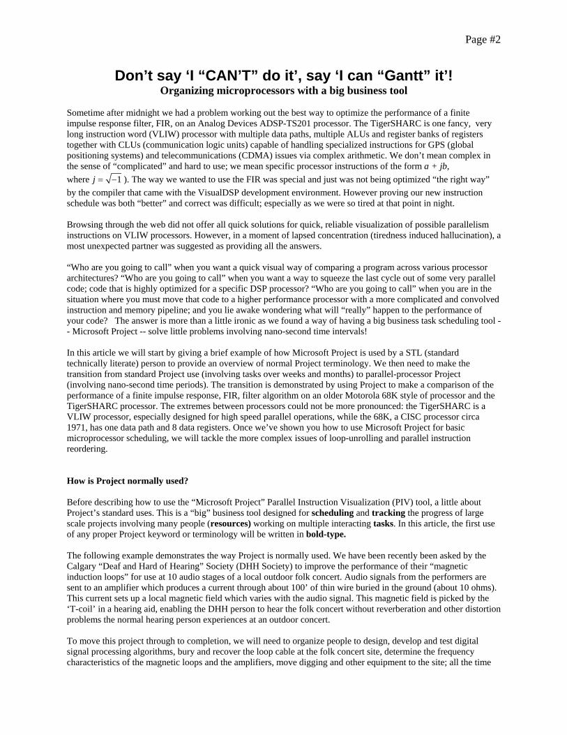
remembering the need to organize preoperational meetings to familiarize the volunteers. A complication is that Mike is the only person with a truck (to move the equipment) and with enough knowledge to familiarize the volunteers. Some of these tasks can be done in parallel and others can only be started after others have completed. Some tasks can be speeded up by having many people working on the project; others will be initially slowed down as the new people need to be trained before they can become productive. Microsoft Project enables you, in a graphical manner, set up the tasks and the relationship between tasks and then demonstrates the time impact of allocating more or less people to various tasks and rescheduling the tasks. Various scenarios can be simulated so the best out of a selection of approaches can be chosen and key components, the critical path, identified. The project leveling tool would be used at some stage during the planning to ensure that no sub trade was assigned to more than one task at the same time during the project duration. Using Microsoft Project In this section we will show how to use Project in a normal way before attempting to “tweak” it to work with nano-second microprocessor tasks. Setting up Microsoft Project to handle task scheduling is fairly straight forward. First, use the Project Wizard to define a project with a known start date (1st August 2006) and all the task names associated with designing and using the magnetic induction loop at the folk concert into the scheduling page (Gantt chart). Now we have to add some information about the task order into the project Gantt chart. Certain tasks MUST occur after other tasks have been completed. These task dependencies are introduced into the Microsoft project by generating links between the tasks. A link is produced by clicking over the task bar (blue) of the first task and dragging the cursor down to the task bar of the second task. A Finish-to-Start (FS) link is the default dependency; with the first task finishing before the second one starts. However Project also permits the use of a delayed Finish-to-Start link (FS + 3Days) to describe a second task that must start at least 3 days after the first completes, or a Start-to-Start link (SS) to describe where it is permitted for two tasks to start and continue at the same time. Note that the word to describe links is “permitted” and not “required”. After use of the resource usage leveling tool, Project may decide that the best way of handling a project with a (FS + 3D) link with be to delay the second task by 7 days rather than just 3 days. This decision making ability is why you pay the big bucks for Project! Having just a series of blue task bars in a Gantt chart is analogous to having undocumented code. We can use the menu option FORMAT | Bar styles |Task | Text | Left and enter Name to allow the details to appear to the side of the task bars on the Gantt chart. Predecessor or other information can be added to the Gantt chart if desired. We can easily see the relationships between the various sub-projects by changing the Gantt chart format using indentation, performed using the green indent arrow in the menu bar. We have also specified the duration needed to complete each task (in days). There are some other issues of task management that have also been handled when preparing Fig. 1. We have filled in the resource column which indicates which organizer is handling each task (ANDREW and MIKE), and activated the Project leveling tool to ensure that no person will have to do two things at the same time.

Page #4

Fig. 1 Here all the interdependencies between the tasks have been introduced by adding links between the project tasks together with the resource name of the person performing the task. Durations of tasks have been added and sub-components of the project can be identified by highlighting a group of task and using the indent icon. Finally the project was leveled so that nobody was performing two tasks at one time. Basic digital signal processing example With the “normal” use of Project demonstrated, we need a digital signal processing example to show how to tweak the Microsoft Project business tool into becoming PIV, the “Microsoft Project” Parallel Instruction Visualization tool. Implementing a finite impulse response (FIR) filter is probably as good a starting point as any. FIR algorithms provide a fairly straight forward technique for filtering a series of input samples to reduce noise or unwanted signal components. Essentially the FIR filtered output is a weighted sum of the last N input values. We have N points of an input signal array 1 2 3, , ..... Nx x x x which we must filter with the FIR filter coefficient array 1 2 3, , ..... Na a a a using the filter (convolution) equation

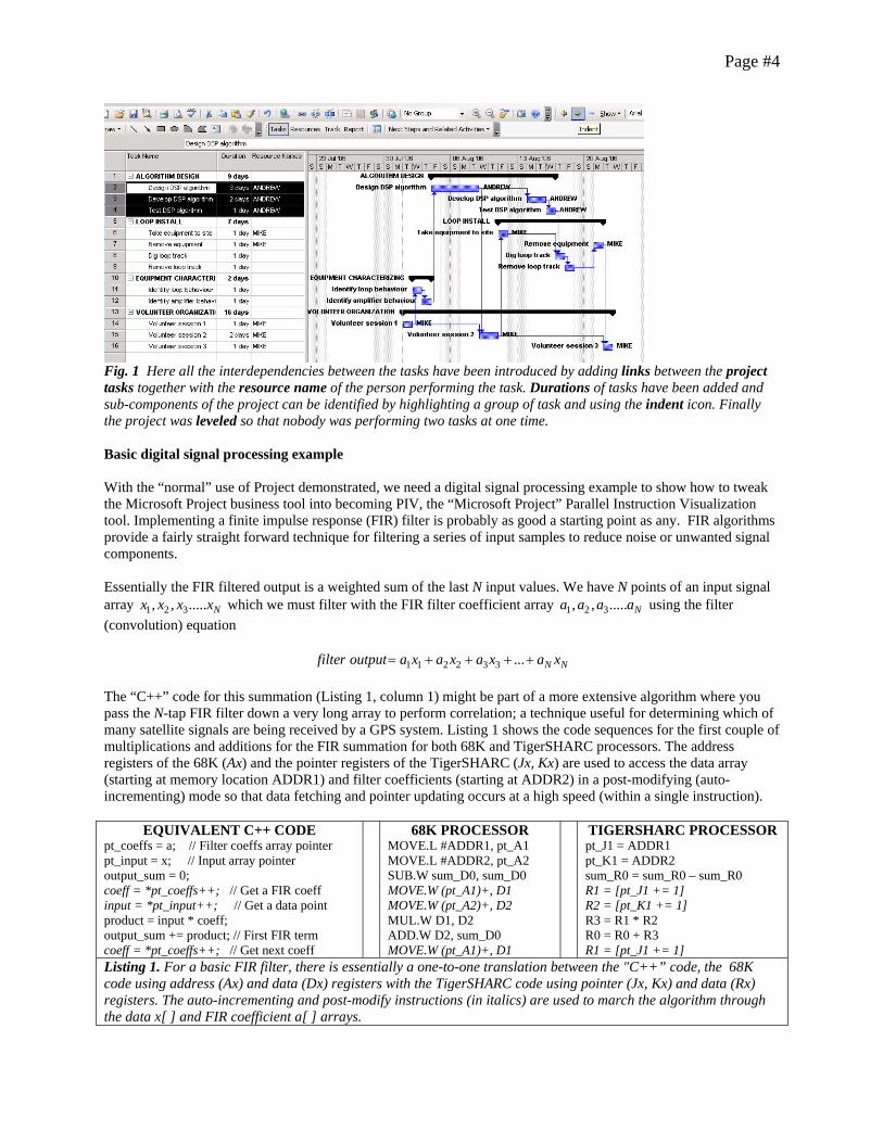
1 1 2 2 3 3 ... N Nfilter output a x a x a x a x= + + + + The “C++” code for this summation (Listing 1, column 1) might be part of a more extensive algorithm where you pass the N-tap FIR filter down a very long array to perform correlation; a technique useful for determining which of many satellite signals are being received by a GPS system. Listing 1 shows the code sequences for the first couple of multiplications and additions for the FIR summation for both 68K and TigerSHARC processors. The address registers of the 68K (Ax) and the pointer registers of the TigerSHARC (Jx, Kx) are used to access the data array (starting at memory location ADDR1) and filter coefficients (starting at ADDR2) in a post-modifying (auto-incrementing) mode so that data fetching and pointer updating occurs at a high speed (within a single instruction).

EQUIVALENT C++ CODE pt_coeffs = a; // Filter coeffs array pointer pt_input = x; // Input array pointer output_sum = 0; coeff = *pt_coeffs++; // Get a FIR coeff input = *pt_input++; // Get a data point product = input * coeff; output_sum += product; // First FIR term coeff = *pt_coeffs++; // Get next coeff

68K PROCESSOR MOVE.L #ADDR1, pt_A1 MOVE.L #ADDR2, pt_A2 SUB.W sum_D0, sum_D0 MOVE.W (pt_A1)+, D1 MOVE.W (pt_A2)+, D2 MUL.W D1, D2 ADD.W D2, sum_D0 MOVE.W (pt_A1)+, D1

TIGERSHARC PROCESSOR pt_J1 = ADDR1 pt_K1 = ADDR2 sum_R0 = sum_R0 – sum_R0 R1 = [pt_J1 += 1] R2 = [pt_K1 += 1] R3 = R1 * R2 R0 = R0 + R3 R1 = [pt_J1 += 1]

Listing 1. For a basic FIR filter, there is essentially a one-to-one translation between the "C++” code, the 68K code using address (Ax) and data (Dx) registers with the TigerSHARC code using pointer (Jx, Kx) and data (Rx) registers. The auto-incrementing and post-modify instructions (in italics) are used to march the algorithm through the data x[ ] and FIR coefficient a[ ] arrays.

Page #5

Microsoft Project, with its tasks, days and linkages, was not designed for handling nano-second microprocessor operations. To make it work in this environment requires some faith and a lot of imagination. First, use the Project Wizard to define a program (project) with a known starting time (a “very future” start date of 1st January 2012 proves to be convenient). Next we use the wizard to inform Project 2003 that the processor (resource-team) will never go into a low power sleep mode (Work schedule is Sunday through Saturday rather than just during week days; Monday through Friday.) Next we cut-and-paste the instructions (tasks) from our assembly source code file (Listing 1) into the instruction scheduling page (Microsoft Project Gantt chart) and start adding information about the processor architectures.

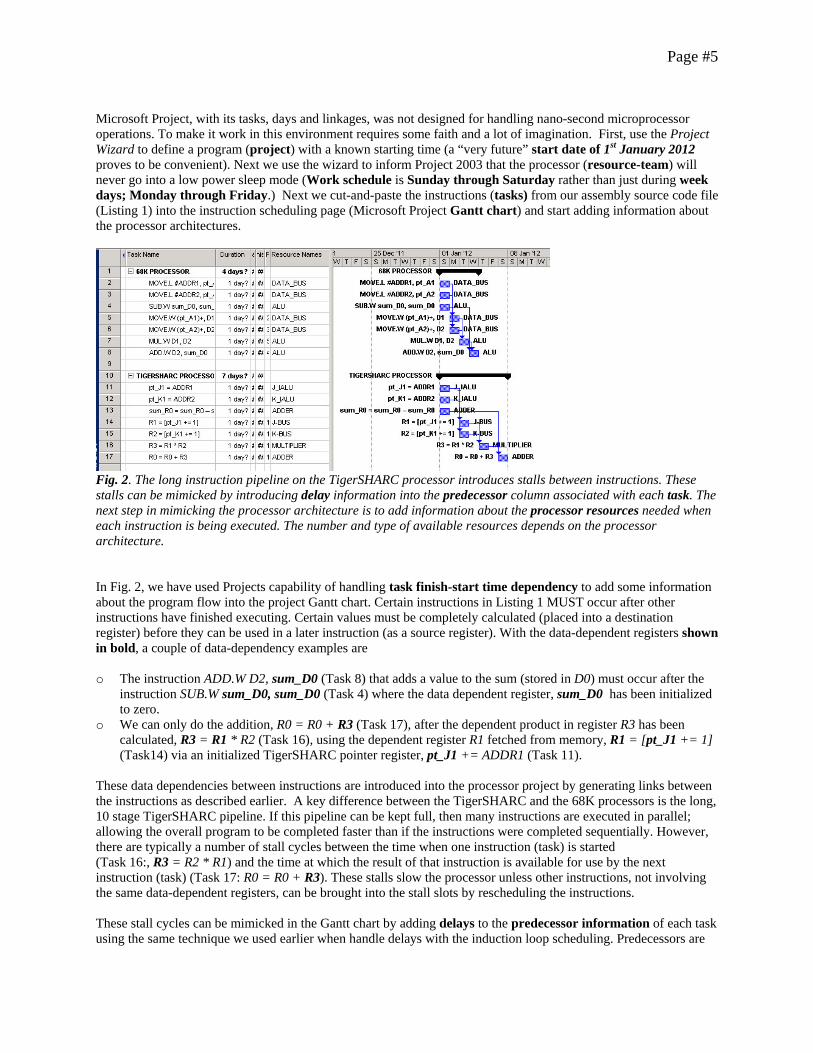
Fig. 2. The long instruction pipeline on the TigerSHARC processor introduces stalls between instructions. These stalls can be mimicked by introducing delay information into the predecessor column associated with each task. The next step in mimicking the processor architecture is to add information about the processor resources needed when each instruction is being executed. The number and type of available resources depends on the processor architecture. In Fig. 2, we have used Projects capability of handling task finish-start time dependency to add some information about the program flow into the project Gantt chart. Certain instructions in Listing 1 MUST occur after other instructions have finished executing. Certain values must be completely calculated (placed into a destination register) before they can be used in a later instruction (as a source register). With the data-dependent registers shown in bold, a couple of data-dependency examples are o The instruction ADD.W D2, sum_D0 (Task 8) that adds a value to the sum (stored in D0) must occur after the

instruction SUB.W sum_D0, sum_D0 (Task 4) where the data dependent register, sum_D0 has been initialized to zero.

o We can only do the addition, R0 = R0 + R3 (Task 17), after the dependent product in register R3 has been calculated, R3 = R1 * R2 (Task 16), using the dependent register R1 fetched from memory, R1 = [pt_J1 += 1] (Task14) via an initialized TigerSHARC pointer register, pt_J1 += ADDR1 (Task 11).

These data dependencies between instructions are introduced into the processor project by generating links between the instructions as described earlier. A key difference between the TigerSHARC and the 68K processors is the long, 10 stage TigerSHARC pipeline. If this pipeline can be kept full, then many instructions are executed in parallel; allowing the overall program to be completed faster than if the instructions were completed sequentially. However, there are typically a number of stall cycles between the time when one instruction (task) is started (Task 16:, R3 = R2 * R1) and the time at which the result of that instruction is available for use by the next instruction (task) (Task 17: R0 = R0 + R3). These stalls slow the processor unless other instructions, not involving the same data-dependent registers, can be brought into the stall slots by rescheduling the instructions. These stall cycles can be mimicked in the Gantt chart by adding delays to the predecessor information of each task using the same technique we used earlier when handle delays with the induction loop scheduling. Predecessors are

Page #6

the early tasks that must be finished before the current task (instruction) can be started. The 68K instruction MOVE.W (pt_A1)+, D1 (Task 5) is dependent on MOVE.L #ADDR1 (Task 2). By contrast the TigerSHARC instruction R1 = [pt_J1 += 1] (Task 14) is dependent on pt_J1= ADDR1 (Task 11) in a more complicated way. The expression 11FS + 1 day in the predecessor column indicates that the finish (F) of Task 11 and the start (S) of Task 14 are separated by 1 day; or in microprocessor terminology, the TigerSHARC register interlocking logic causes the processor to automatically insert one stall cycle between these instructions to ensure proper processor operation although there are inter-instruction data dependencies. Handling the limited resources present in the 68K and TigerSHARC architectures Investigating the differences between the two processor architectures requires the addition of details about the available internal processor resources using the Resource Names column of the Gantt chart. In Fig. 2, we have indicated which of the 68K instructions uses the DATA_BUS and ALU resources, together with which of the TigerSHARC instructions use the integer ALUs (J-IALU, K-IALU) for address calculations, the two data busses (J-BUS, K-BUS) and the ADDER and MULTIPLIER resources. To keep this problem example manageable, we shall ignore for the moment the fact that there are two compute blocks (X and Y) on the TigerSHARC; each with its own adder, multiplier, shifter and register bank. However, this use of processor resources shown is not realistic. It is possible for the J-bus and K-bus resources on the TigerSHARC to be used independently in the same processor cycle to bring in two data values from two different memory blocks, but the 68K DATA_BUS resource can’t be used twice in one cycle. This problem is solved by leveling the project using the Tools | level resources | level now button to ensure that no resource is being used more than once during each instruction. After leveling the project to ensure the resource usage is correct, new problems appear. It is legal on the TigerSHARC to have a parallel instruction combination pt_K1= ADDR2; sum_R0 = sum_R0 – sum_R0;; However the equivalent 68 K instruction combination MOVE #ADDR1, A1 SUB.W sum_D0, sub_D0 is illegal. In addition, Project is indicating a possible highly parallel, triple TigerSHARC instruction pt_J1 = ADDR1; pt_J2 = ADDR2; R0 = R0 – R0;; It is possible to execute four simultaneous instructions on the TigerSHARC; but this particular one is illegal. The first two TigerSHARC instructions require 64 bits and the third instruction requires 32 bits for a total of 160 bits; impossible to handle in a single cycle on the 128-bit TigerSHARC instruction bus. These problems can be solved by adding to the Gantt chart the fact that all the 68K instructions make use of the register block resource REG_BLOCK, while the immediate TigerSHARC instructions of the form pt_J1 = ADDR1; make use of the IMEX (immediate extended) capability of the processor. However, as can be seen Fig. 3, adding this new resource information and leveling the project does not produce the expected result. Although we have now solved the overly parallel instruction issue seen earlier, we have introduced a new problem - many of the tasks now take half a cycle to complete! We have met the first problem associated with microprocessor architectural simulation not met by the default configuration of Microsoft Project – that’s not a bad track record when pushing a big business tool into a place where it was not designed to go!

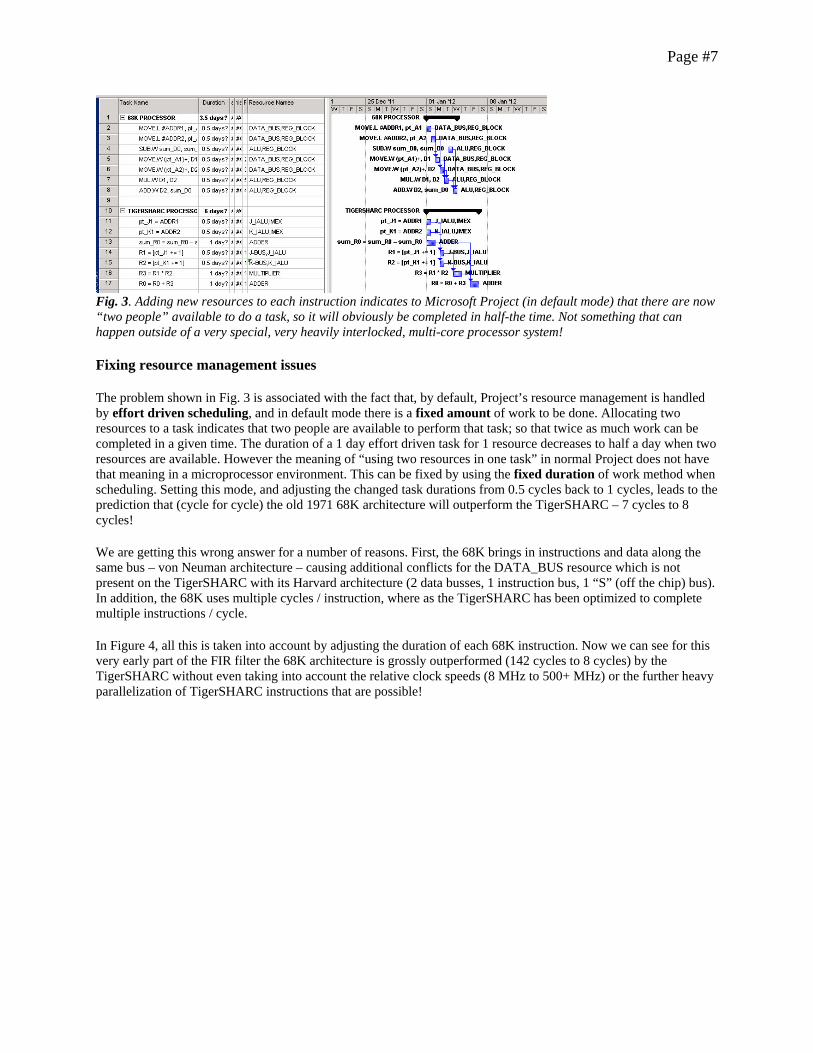
Page #7

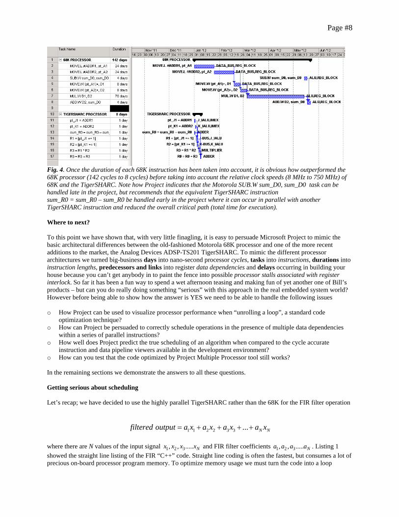
Fig. 3. Adding new resources to each instruction indicates to Microsoft Project (in default mode) that there are now “two people” available to do a task, so it will obviously be completed in half-the time. Not something that can happen outside of a very special, very heavily interlocked, multi-core processor system! Fixing resource management issues The problem shown in Fig. 3 is associated with the fact that, by default, Project’s resource management is handled by effort driven scheduling, and in default mode there is a fixed amount of work to be done. Allocating two resources to a task indicates that two people are available to perform that task; so that twice as much work can be completed in a given time. The duration of a 1 day effort driven task for 1 resource decreases to half a day when two resources are available. However the meaning of “using two resources in one task” in normal Project does not have that meaning in a microprocessor environment. This can be fixed by using the fixed duration of work method when scheduling. Setting this mode, and adjusting the changed task durations from 0.5 cycles back to 1 cycles, leads to the prediction that (cycle for cycle) the old 1971 68K architecture will outperform the TigerSHARC – 7 cycles to 8 cycles! We are getting this wrong answer for a number of reasons. First, the 68K brings in instructions and data along the same bus – von Neuman architecture – causing additional conflicts for the DATA_BUS resource which is not present on the TigerSHARC with its Harvard architecture (2 data busses, 1 instruction bus, 1 “S” (off the chip) bus). In addition, the 68K uses multiple cycles / instruction, where as the TigerSHARC has been optimized to complete multiple instructions / cycle. In Figure 4, all this is taken into account by adjusting the duration of each 68K instruction. Now we can see for this very early part of the FIR filter the 68K architecture is grossly outperformed (142 cycles to 8 cycles) by the TigerSHARC without even taking into account the relative clock speeds (8 MHz to 500+ MHz) or the further heavy parallelization of TigerSHARC instructions that are possible!

Page #8

Fig. 4. Once the duration of each 68K instruction has been taken into account, it is obvious how outperformed the 68K processor (142 cycles to 8 cycles) before taking into account the relative clock speeds (8 MHz to 750 MHz) of 68K and the TigerSHARC. Note how Project indicates that the Motorola SUB.W sum_D0, sum_D0 task can be handled late in the project, but recommends that the equivalent TigerSHARC instruction sum_R0 = sum_R0 – sum_R0 be handled early in the project where it can occur in parallel with another TigerSHARC instruction and reduced the overall critical path (total time for execution). Where to next? To this point we have shown that, with very little finagling, it is easy to persuade Microsoft Project to mimic the basic architectural differences between the old-fashioned Motorola 68K processor and one of the more recent additions to the market, the Analog Devices ADSP-TS201 TigerSHARC. To mimic the different processor architectures we turned big-business days into nano-second processor cycles, tasks into instructions, durations into instruction lengths, predecessors and links into register data dependencies and delays occurring in building your house because you can’t get anybody in to paint the fence into possible processor stalls associated with register interlock. So far it has been a fun way to spend a wet afternoon teasing and making fun of yet another one of Bill’s products – but can you do really doing something “serious” with this approach in the real embedded system world? However before being able to show how the answer is YES we need to be able to handle the following issues o How Project can be used to visualize processor performance when “unrolling a loop”, a standard code

optimization technique? o How can Project be persuaded to correctly schedule operations in the presence of multiple data dependencies

within a series of parallel instructions? o How well does Project predict the true scheduling of an algorithm when compared to the cycle accurate

instruction and data pipeline viewers available in the development environment? o How can you test that the code optimized by Project Multiple Processor tool still works? In the remaining sections we demonstrate the answers to all these questions. Getting serious about scheduling Let’s recap; we have decided to use the highly parallel TigerSHARC rather than the 68K for the FIR filter operation

1 1 2 2 3 3 ... N Nfiltered output a x a x a x a x= + + + + where there are N values of the input signal 1 2 3, , ..... Nx x x x and FIR filter coefficients 1 2 3, , ..... Na a a a . Listing 1 showed the straight line listing of the FIR “C++” code. Straight line coding is often the fastest, but consumes a lot of precious on-board processor program memory. To optimize memory usage we must turn the code into a loop

Page #9

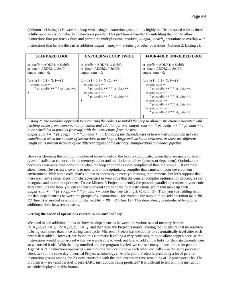
(Column 1: Listing 2) However, a loop with a single instruction group in it is highly inefficient speed wise as there is little opportunity to make the instructions parallel. This problem is handled by unfolding the loop to allow instructions that pre-fetch values and permit the multiplication q p pproduct input coeff= × operations to overlap with

instructions that handle the earlier addition _ q qoutput sum product+ = or other operations (Column 2: Listing 2).

STANDARD LOOP pt_coeffs = ADDR1; // &a[0]; pt_data = ADDR2; // &x[0]; output_sum = 0; for (int i = 0; i < N; i++) { output_sum += * pt_coeffs ++ * * pt_data ++; }

UNFOLDING LOOP TWICE pt_coeffs = ADDR1; // &a[0]; pt_data = ADDR2; // &x[0]; output_sum = 0; for (int i = 0; i < N / 2; i++) { output_sum += * pt_coeffs ++ * * pt_data ++; output_sum += * pt_coeffs ++ * * pt_data ++; }

FOUR-FOLD UNFOLDED LOOP pt_coeffs = ADDR1; // &a[0]; pt_data = ADDR2; // &x[0]; output_sum = 0; for (int i = 0; i < N; i++) { output_sum += * pt_coeffs ++ * * pt_data ++; output_sum += * pt_coeffs ++ * * pt_data ++; output_sum += * pt_coeffs ++ * * pt_data ++; output_sum += * pt_coeffs ++ * * pt_data ++; }

Listing 2: The standard approach to optimizing the code is to unfold the loop to allow instructions associated with fetching values from memory, multiplication and addition for one output_sum += * pt_coeffs ++ * * pt_data ++;; to be scheduled in parallel (overlap) with the instructions from the next output_sum += * pt_coeffs ++ * * pt_data ++;;. Handling the dependencies between instructions can get very complicated when the number of instructions in the loop is large and varied in structure, or there are different length stalls present because of the different depths of the memory, multiplication and adder pipeline. However choosing the optimum number of times to unfold the loop is complicated when there are many different types of stalls that can occur in the memory, adder and multiplier pipelines (processor dependent). Optimization becomes even more time-consuming when the loop structure is more complicated than the simple FIR example shown here. The easiest answer is to now turn on the optimizing compiler that came with your development environment. With some code, that’s all that is necessary to meet your timing requirements, but let’s suppose that there are many special algorithm characteristics in your code that the general compiler optimization procedures can’t recognize and therefore optimize. To use Microsoft Project to identify the possible parallel operations in your code after unrolling the loop, you cut and paste several copies of the four instructions group that make up each output_sum += * pt_coeffs ++ * * pt_data ++;code line (see Listing 2, Column 2). Then you start adding in all the data dependencies between the groups of 4 instructions – for example the output of one add operation R0 = R0 + R3 (line 8) is needed as an input for the next R0 = R0 + R3 (line 12). This dependency is introduced by adding additional links between the tasks. Getting the order of operations correct in an unrolled loop We need to add additional links to show the dependencies between the various sets of memory fetches R1 = [pt_J1 += 1], R2 = [pt_K1 += 1], and then used the Project resource leveling tool to ensure that no resource is being used more than once during each cycle. Microsoft Project has the ability to automatically level after each new task is added. However, we found this automatic levelling a very confusing thing to allow happen because the instructions would jump around while we were trying to work out how to add all the links for the data dependencies; so we turned it off. With the loop unrolled and the program leveled, we can see many opportunities for parallel TigerSHARC instructions appearing – instructions that occur above each other vertically – in the same processor clock tick (in the same day in normal Project terminology). At this point, Project is predicting a lot of parallel instruction groups among the 23 instructions but with the total execution time remaining at 12 processor ticks. The problem is – are valid parallel TigerSHARC instructions being predicted? It is difficult to tell with the instruction schedule displayed in this format.

Page #10

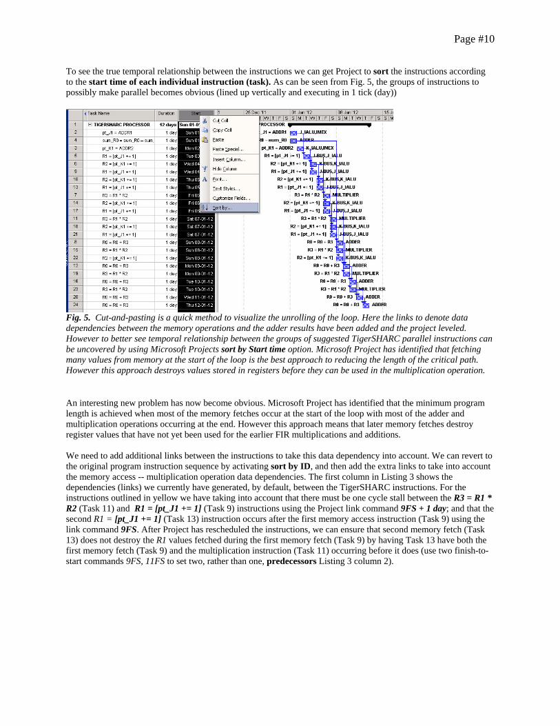
To see the true temporal relationship between the instructions we can get Project to sort the instructions according to the start time of each individual instruction (task). As can be seen from Fig. 5, the groups of instructions to possibly make parallel becomes obvious (lined up vertically and executing in 1 tick (day))

Fig. 5. Cut-and-pasting is a quick method to visualize the unrolling of the loop. Here the links to denote data dependencies between the memory operations and the adder results have been added and the project leveled. However to better see temporal relationship between the groups of suggested TigerSHARC parallel instructions can be uncovered by using Microsoft Projects sort by Start time option. Microsoft Project has identified that fetching many values from memory at the start of the loop is the best approach to reducing the length of the critical path. However this approach destroys values stored in registers before they can be used in the multiplication operation. An interesting new problem has now become obvious. Microsoft Project has identified that the minimum program length is achieved when most of the memory fetches occur at the start of the loop with most of the adder and multiplication operations occurring at the end. However this approach means that later memory fetches destroy register values that have not yet been used for the earlier FIR multiplications and additions. We need to add additional links between the instructions to take this data dependency into account. We can revert to the original program instruction sequence by activating sort by ID, and then add the extra links to take into account the memory access -- multiplication operation data dependencies. The first column in Listing 3 shows the dependencies (links) we currently have generated, by default, between the TigerSHARC instructions. For the instructions outlined in yellow we have taking into account that there must be one cycle stall between the R3 = R1 * R2 (Task 11) and R1 = [pt_J1 += 1] (Task 9) instructions using the Project link command 9FS + 1 day; and that the second R1 = [pt_J1 += 1] (Task 13) instruction occurs after the first memory access instruction (Task 9) using the link command 9FS. After Project has rescheduled the instructions, we can ensure that second memory fetch (Task 13) does not destroy the R1 values fetched during the first memory fetch (Task 9) by having Task 13 have both the first memory fetch (Task 9) and the multiplication instruction (Task 11) occurring before it does (use two finish-to-start commands 9FS, 11FS to set two, rather than one, predecessors Listing 3 column 2).

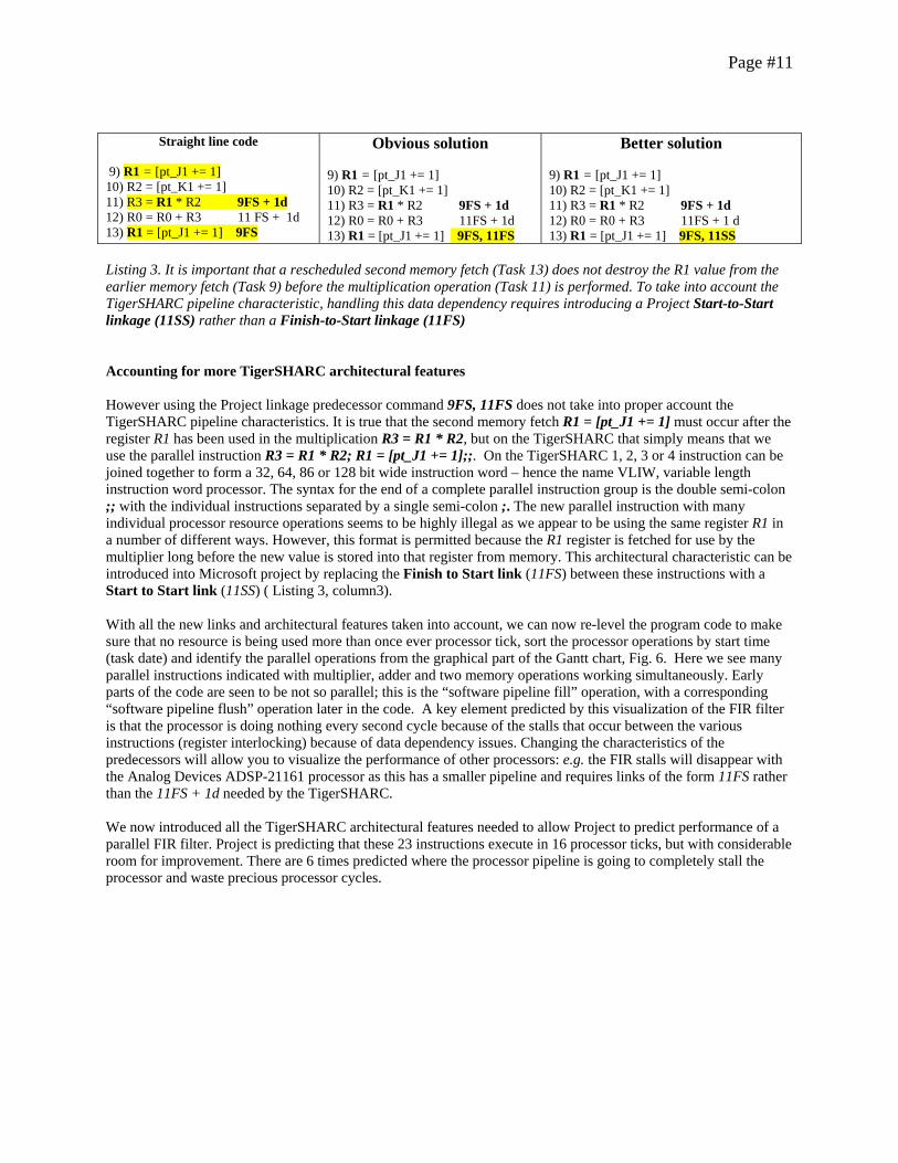
Page #11

Listing 3. It is important that a rescheduled second memory fetch (Task 13) does not destroy the R1 value from the earlier memory fetch (Task 9) before the multiplication operation (Task 11) is performed. To take into account the TigerSHARC pipeline characteristic, handling this data dependency requires introducing a Project Start-to-Start linkage (11SS) rather than a Finish-to-Start linkage (11FS) Accounting for more TigerSHARC architectural features However using the Project linkage predecessor command 9FS, 11FS does not take into proper account the TigerSHARC pipeline characteristics. It is true that the second memory fetch R1 = [pt_J1 += 1] must occur after the register R1 has been used in the multiplication R3 = R1 * R2, but on the TigerSHARC that simply means that we use the parallel instruction R3 = R1 * R2; R1 = [pt_J1 += 1];;. On the TigerSHARC 1, 2, 3 or 4 instruction can be joined together to form a 32, 64, 86 or 128 bit wide instruction word – hence the name VLIW, variable length instruction word processor. The syntax for the end of a complete parallel instruction group is the double semi-colon ;; with the individual instructions separated by a single semi-colon ;. The new parallel instruction with many individual processor resource operations seems to be highly illegal as we appear to be using the same register R1 in a number of different ways. However, this format is permitted because the R1 register is fetched for use by the multiplier long before the new value is stored into that register from memory. This architectural characteristic can be introduced into Microsoft project by replacing the Finish to Start link (11FS) between these instructions with a Start to Start link (11SS) ( Listing 3, column3). With all the new links and architectural features taken into account, we can now re-level the program code to make sure that no resource is being used more than once ever processor tick, sort the processor operations by start time (task date) and identify the parallel operations from the graphical part of the Gantt chart, Fig. 6. Here we see many parallel instructions indicated with multiplier, adder and two memory operations working simultaneously. Early parts of the code are seen to be not so parallel; this is the “software pipeline fill” operation, with a corresponding “software pipeline flush” operation later in the code. A key element predicted by this visualization of the FIR filter is that the processor is doing nothing every second cycle because of the stalls that occur between the various instructions (register interlocking) because of data dependency issues. Changing the characteristics of the predecessors will allow you to visualize the performance of other processors: e.g. the FIR stalls will disappear with the Analog Devices ADSP-21161 processor as this has a smaller pipeline and requires links of the form 11FS rather than the 11FS + 1d needed by the TigerSHARC. We now introduced all the TigerSHARC architectural features needed to allow Project to predict performance of a parallel FIR filter. Project is predicting that these 23 instructions execute in 16 processor ticks, but with considerable room for improvement. There are 6 times predicted where the processor pipeline is going to completely stall the processor and waste precious processor cycles.

Straight line code 9) R1 = [pt_J1 += 1] 10) R2 = [pt_K1 += 1] 11) R3 = R1 * R2 9FS + 1d 12) R0 = R0 + R3 11 FS + 1d 13) R1 = [pt_J1 += 1] 9FS

Obvious solution 9) R1 = [pt_J1 += 1] 10) R2 = [pt_K1 += 1] 11) R3 = R1 * R2 9FS + 1d 12) R0 = R0 + R3 11FS + 1d 13) R1 = [pt_J1 += 1] 9FS, 11FS

Better solution 9) R1 = [pt_J1 += 1] 10) R2 = [pt_K1 += 1] 11) R3 = R1 * R2 9FS + 1d 12) R0 = R0 + R3 11FS + 1 d 13) R1 = [pt_J1 += 1] 9FS, 11SS

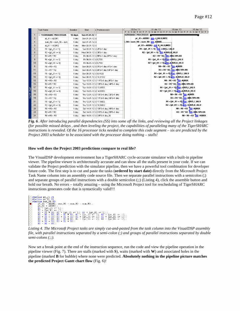
Page #12

Fig. 6. After introducing parallel dependencies (SS) into some ofl the links, and reviewing all the Project linkages (for possible missed delays , and then leveling the project, the capabilities of paralleling many of the TigerSHARC instructions is revealed. Of the 16 processor ticks needed to complete this code segment – six are predicted by the Project 2003 scheduler to be associated with the processor doing nothing – stalls! How well does the Project 2003 predictions compare to real life? The VisualDSP development environment has a TigerSHARC cycle-accurate simulator with a built-in pipeline viewer. The pipeline viewer is architecturally accurate and can show all the stalls present in your code. If we can validate the Project prediction with the simulator pipeline, then we have a powerful tool combination for developer future code. The first step is to cut and paste the tasks (ordered by start date) directly from the Microsoft Project Task Name column into an assembly code source file. Then we separate parallel instructions with a semicolon (;) and separate groups of parallel instructions with a double semicolon (;;) (Listing 4), click the assemble button and hold our breath. No errors – totally amazing – using the Microsoft Project tool for rescheduling of TigerSHARC instructions generates code that is syntactically valid!!!

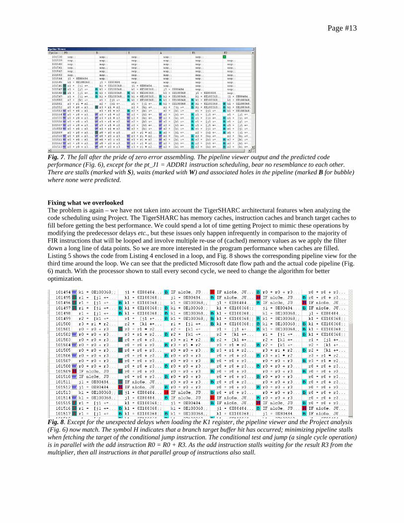
Listing 4. The Microsoft Project tasks are simply cut-and-pasted from the task column into the VisualDSP assembly file, with parallel instructions separated by a semi-colon (;) and groups of parallel instructions separated by double semi-colons (;;). Now set a break point at the end of the instruction sequence, run the code and view the pipeline operation in the pipeline viewer (Fig. 7). There are stalls (marked with S), waits (marked with W) and associated holes in the pipeline (marked B for bubble) where none were predicted. Absolutely nothing in the pipeline picture matches the predicted Project Gantt chart flow (Fig. 6)!

Page #13

Fig. 7. The fall after the pride of zero error assembling. The pipeline viewer output and the predicted code performance (Fig. 6), except for the pt_J1 = ADDR1 instruction scheduling, bear no resemblance to each other. There are stalls (marked with S), waits (marked with W) and associated holes in the pipeline (marked B for bubble) where none were predicted. Fixing what we overlooked The problem is again – we have not taken into account the TigerSHARC architectural features when analyzing the code scheduling using Project. The TigerSHARC has memory caches, instruction caches and branch target caches to fill before getting the best performance. We could spend a lot of time getting Project to mimic these operations by modifying the predecessor delays etc., but these issues only happen infrequently in comparison to the majority of FIR instructions that will be looped and involve multiple re-use of (cached) memory values as we apply the filter down a long line of data points. So we are more interested in the program performance when caches are filled. Listing 5 shows the code from Listing 4 enclosed in a loop, and Fig. 8 shows the corresponding pipeline view for the third time around the loop. We can see that the predicted Microsoft date flow path and the actual code pipeline (Fig. 6) match. With the processor shown to stall every second cycle, we need to change the algorithm for better optimization.

Fig. 8. Except for the unexpected delays when loading the K1 register, the pipeline viewer and the Project analysis (Fig. 6) now match. The symbol H indicates that a branch target buffer hit has occurred; minimizing pipeline stalls when fetching the target of the conditional jump instruction. The conditional test and jump (a single cycle operation) is in parallel with the add instruction R0 = R0 + R3. As the add instruction stalls waiting for the result R3 from the multiplier, then all instructions in that parallel group of instructions also stall.

Page #14

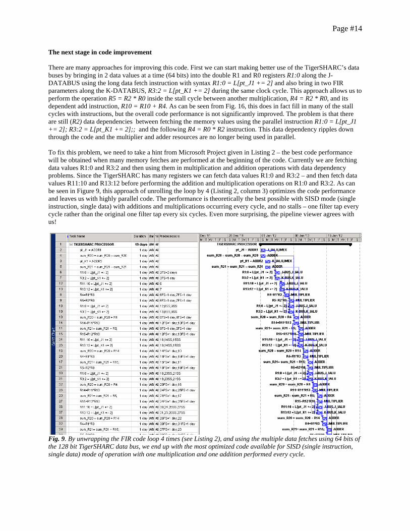
The next stage in code improvement There are many approaches for improving this code. First we can start making better use of the TigerSHARC’s data buses by bringing in 2 data values at a time (64 bits) into the double R1 and R0 registers R1:0 along the J-DATABUS using the long data fetch instruction with syntax R1:0 = L[pt_J1 += 2] and also bring in two FIR parameters along the K-DATABUS, R3:2 = L[pt_K1 += 2] during the same clock cycle. This approach allows us to perform the operation R5 = R2 * R0 inside the stall cycle between another multiplication, R4 = R2 * R0, and its dependent add instruction, R10 = R10 + R4. As can be seen from Fig. 16, this does in fact fill in many of the stall cycles with instructions, but the overall code performance is not significantly improved. The problem is that there are still (R2) data dependencies between fetching the memory values using the parallel instruction R1:0 = L[pt_J1 += 2]; R3:2 = L[pt_K1 += 2];; and the following R4 = R0 * R2 instruction. This data dependency ripples down through the code and the multiplier and adder resources are no longer being used in parallel. To fix this problem, we need to take a hint from Microsoft Project given in Listing 2 – the best code performance will be obtained when many memory fetches are performed at the beginning of the code. Currently we are fetching data values R1:0 and R3:2 and then using them in multiplication and addition operations with data dependency problems. Since the TigerSHARC has many registers we can fetch data values R1:0 and R3:2 – and then fetch data values R11:10 and R13:12 before performing the addition and multiplication operations on R1:0 and R3:2. As can be seen in Figure 9, this approach of unrolling the loop by 4 (Listing 2, column 3) optimizes the code performance and leaves us with highly parallel code. The performance is theoretically the best possible with SISD mode (single instruction, single data) with additions and multiplications occurring every cycle, and no stalls – one filter tap every cycle rather than the original one filter tap every six cycles. Even more surprising, the pipeline viewer agrees with us!

Fig. 9. By unwrapping the FIR code loop 4 times (see Listing 2), and using the multiple data fetches using 64 bits of the 128 bit TigerSHARC data bus, we end up with the most optimized code available for SISD (single instruction, single data) mode of operation with one multiplication and one addition performed every cycle.

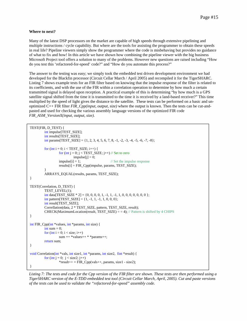
Page #15

TEST(FIR, D_TEST) { int impulse[TEST_SIZE]; int results[TEST_SIZE]; int params[TEST_SIZE] = {1, 2, 3, 4, 5, 6, 7, 8, -1, -2, -3, -4, -5, -6, -7, -8}; for (int i = 0; i < TEST_SIZE; i++) { for (int j = 0; j < TEST_SIZE; j++) // Set to zero impulse[j] = 0; impulse[i] = 1; // Set the impulse response results[i] = FIR_Cpp(impulse, params, TEST_SIZE); } ARRAYS_EQUAL(results, params, TEST_SIZE); } TEST(Correlation, D_TEST) { TEST_LEVEL(1); int data[TEST_SIZE * 2] = {0, 0, 0, 0, 1, -1, 1, -1, 1, 0, 0, 0, 0, 0, 0, 0 }; int pattern[TEST_SIZE] = {1, -1, 1, -1, 1, 0, 0, 0}; int result[TEST_SIZE]; Correllation(data, 2 * TEST_SIZE, pattern, TEST_SIZE, result); CHECK(MaximumLocation(result, TEST_SIZE) = = 4); // Pattern is shifted by 4 CHIPS } int FIR_Cpp(int *values, int *params, int size) { int sum = 0; for (int i = 0; i < size; i++) sum += *values++ * *params++; return sum; } void Correlation(int *vals, int size1, int *params, int size2, fint *result) { for (int j = 0; j < size2; j++) *result++ = FIR_Cpp(vals++, params, size1 - size2); }

Where to next? Many of the latest DSP processors on the market are capable of high speeds through extensive pipelining and multiple instructions / cycle capability. But where are the tools for assisting the programmer to obtain these speeds in real life? Pipeline viewers simply show the programmer where the code is misbehaving but provides no guidance of what to fix and how! In this article we have shown how combining the pipeline viewer with the big business Microsoft Project tool offers a solution to many of the problems. However new questions are raised including “How do you test this ‘refactored-for-speed’ code?” and “How do you automate this process?” The answer to the testing was easy; we simply took the embedded test driven development environment we had developed for the Blackfin processor (Circuit Cellar March / April 2005) and recompiled it for the TigerSHARC. Listing 7 shows example tests for an FIR filter based on knowing that the impulse response of the filter is related to its coefficients, and with the use of the FIR within a correlation operation to determine by how much a certain transmitted signal is delayed upon reception. A practical example of this is determining “by how much is a GPS satellite signal shifted from the time it is transmitted to the time it is received by a land-based receiver?” This time multiplied by the speed of light gives the distance to the satellite. These tests can be performed on a basic and un-optimized C++ FIR filter FIR_Cpp(input, output, size) where the output is known. Then the tests can be cut-and-pasted and used for checking the various assembly language versions of the optimized FIR code FIR_ASM_VersionX(input, output, size).

Listing 7: The tests and code for the Cpp version of the FIR filter are shown. These tests are then performed using a TigerSHARC version of the E-TDD embedded test tool (Circuit Cellar March, April, 2005). Cut and paste versions of the tests can be used to validate the “refactored-for-speed” assembly code.

Page #16

Answering the question about “automation” requires knowledge of where do you think you want to go? We have not discussed the issue of taking the optimized “unrolled” loop code and rearranging it (software pipelining) to have the twin advantages of highly efficient parallel code throughout a loop that has been optimized for memory usage. We have not even started demonstrating how to add to Project all the possible features for high performance on the most recent DSP processors – dual compute blocks so that two 32-bit additions and two 32-bit multiplications combined with two QUAD (128-bit) memory fetches in a single single-instruction double-memory (SIMD) cycle for a start. Then there is the ability to do complex multiplication (a + jb) * (c + jd) on 16-bit complex values in a single cycle using instructions of the form R1 = R2 ** R3 or even 64 taps of a complex correlation (16-bit with 1-bit) in a single instruction XCORRS. Part of the answer to this question is “let the C++ compiler do some of the optimizing for us”. However, with a more difficult problem than FIR filtering, the general optimization performed with the C++ compiler is not going to be enough. This means we need to take the highly optimized and very parallel code from the C++ compiler and place that code into Project for further examination via a parsing tool with knowledge of the processor architecture and capable of reformating the compiler output. That’s not a five minute job, especially if we want the tool to be able to handle the different architectural capabilities of different processors. We will leave the solution to that issue to a later time. Part of this work is a technical transfer activity related to a collaborative grant funded by Analog Devices and Natural Sciences and Engineering Research Council of Canada (NSERC). About the authors Mike Smith has been writing computer-related articles since the mid ‘70s. He is a professor in Electrical and Computer Engineering at the University of Calgary, Canada. Amongst his interests are the development and testing of algorithms for real-time analysis of stroke images from magnetic resonance imaging. He has recently started to use test driven development and FIT techniques to formalize the testing techniques for embedded system software he has always used. He has received the Analog Devices University Ambassadorship award since 2002. Mike can be contacted at smithmr@ucalgary.ca James Miller is a professor in Electrical and Computer Engineering at the University of Alberta, Canada. In addition to developing small self-contained embedded systems for health monitoring, he has interests in efficient software testing procedures to ensure quality. James can be contacted at jm@ece.ualberta.ca