Horn 1

Domestic Well Capture Zone and Influence of the Gravel Pack Length 1

Judith E. Horn and Thomas Harter* 2

Department of Land, Air, and Water Resources 3

University of California 4

Davis, CA 95616-8629 5

• (corresponding author; ThHarter@ucdavis.edu; 530-752-2709) 6

7

Accepted for publication in the journal “Ground Water”, September 2008 8

9

Abstract 10

Domestic wells in North America and elsewhere are typically constructed at relatively shallow 11

depths and with the sand or gravel pack extending far above the intake screen of the well (shallow 12

well seal). The source areas of these domestic wells and the effect of an extended gravel pack on the 13

source area are typically unknown and few resources exist for estimating these. In this paper, we use 14

detailed, high-resolution groundwater modeling to estimate the capture zone (source area) of a 15

typical domestic well located in an alluvial aquifer. Results for a wide range of aquifer and gravel 16

pack hydraulic conductivities are compared to a simple analytical model. Correction factors for the 17

analytical model are computed based on statistical regression of the numerical results against the 18

analytical model. This tool can be applied to estimate the source area of a domestic well for a wide 19

range of conditions. We show that an extended gravel pack above the well screen may contribute 20

significantly to the overall inflow to a domestic well, especially in less permeable aquifers, where 21

that contribution may range from 20% to 50%; and that an extended gravel pack may lead to a 22

significantly elongated capture zone, in some instances nearly doubling the length of the capture 23

Horn 2

zone. Extending the gravel pack much above the intake screen therefore significantly increases the 24

vulnerability of the water source. 25

26

Introduction 27

Most households in rural areas of the United States, outside the service area of incorporated cities, 28

rely on domestic wells for their water supply (McCray 2005, U.S. EPA 1997). And many of these 29

domestic wells are constructed with a well-screen at depth and a sand or gravel pack that extends 30

upward to the mandatory minimum depth of the well seal, which is dictated by local and state 31

guidelines. A question commonly asked by homeowners is: Where does our water come from? The 32

capture zones (also referred to as the source area or recharge area) of domestic wells are rarely 33

determined. Attention has instead focused on public supply wells and their capture zones as these are 34

regulated through U.S. EPA’s source water protection program. Domestic wells, typically serving a 35

single family, are often constructed to relatively shallow depths when compared to public or 36

municipal water supply wells (Burow et al. 2004). 37

38

Methods for delineating well capture zones range from very simple to very complex. In general, the 39

various approaches fall into four categories (Harter, 2008): 40

1. Geometric or graphical methods involve the use of a pre-determined fixed radius without any 41

special consideration of the flow system, or the use of simplified shapes that have been pre-42

calculated for a range of pumping and aquifer conditions. 43

2. Analytical methods allow calculation of distances for protection zones using equations that can be 44

solved using a hand calculator or microcomputer spreadsheet program. 45

Horn 3

3. Hydrogeologic mapping involves identifying the recharge zone and the source zone based on 46

geomorphic, geologic, hydrologic, and hydrochemical characteristics of an aquifer. 47

4. Computer modeling methods involve devising, calibrating, and applying complex analytical or 48

numerical models that simulate groundwater flow and contaminant transport processes. 49

The long-term average pumping rate of domestic wells typically ranges from less than 4 L/min [1 50

gallon/min] to 20 L/min [5 gallon/min]. Using the graphical method employed by California’s 51

Drinking Water Source Assessment and Protection (DWSAP) Program (California DHS, 1999), for 52

example, the default source area of a domestic well pumping 1,233.5 m3/year (1 acre-foot per year, 53

the typical annual consumption of a U.S. single family household) is a circle with a radius of 15 m 54

(~50 ft) for areal recharge of 450 mm/year (typical for very humid areas or rural residences in semi-55

arid areas surrounded by irrigated lawn and fields) or with a radius of 31 m (~100ft) at a recharge 56

rate of 100 mm/year (typical of many semi-arid regions). This simple geometric approach neglects 57

the effects of the regional groundwater flow on the capture zone of a domestic well. 58

59

On the other hand, where regional groundwater flow is dominant and local recharge is negligible, the 60

capture zone of a domestic well can also be easily computed if the well fully penetrates the aquifer 61

system or does not strongly affect regional groundwater flow. The width, w, of the capture zone of a 62

domestic well is then obtained by simple mass balance (Todd 1980): 63

w = Q / (T * i) (1) 64

where Q is the pumping rate, T is the aquifer transmissivity, and i is the regional hydraulic gradient. 65

For example, at a relatively low transmissivity, T, of 10 m2/d, a regional groundwater gradient of 66

0.5% and a pumping rate of 1,233 m3/year, the width of the capture zone is approximately 60 m 67

Horn 4

(~200 feet). At values of T typical for productive aquifers, the width of the capture zone is often on 68

the order of 1 m - 10 m (~ 3 feet - ~30 feet) or even less. 69

70

Both, the geometric approach and equation (1) above provide simple approximations for extremely 71

idealized conditions. Here, our objective is to determine the capture zone of a domestic well with a 72

sand or gravel pack, completed in an unconfined aquifer, where both, recharge and regional 73

groundwater flow are significant. We use high-resolution computer simulations to determine the 74

source area and to explicitly determine the influence of the gravel pack on the well capture zone. For 75

reference, we compare those to a simple analytical model of the capture zone for a low-producing 76

well in an unconfined aquifer with recharge. Our study’s focus is on rural domestic wells in irrigated 77

agricultural regions, e.g., of the Southwestern United States, where significant recharge is due to 78

irrigation return flows and much of the groundwater production is for irrigation purposes. Our 79

findings have general implications that are independent of this particular climate scenario. 80

81

Conceptual Framework 82

Domestic wells in rural areas are assumed to be completed near the uppermost portion of a regional 83

aquifer system. Furthermore, we assume that a significant downward gradient exists in the regional 84

aquifer system due to recharge at the water table and due to significant groundwater production 85

(mostly for irrigation) from the deeper portions of the aquifer system (e.g., Belitz and Phillips, 86

1995). Burow et al. (2004), for example, report typical recharge rates in irrigated areas in the San 87

Joaquin Valley, California, to be on the order of 550 – 750 mm/a with the majority of recharge 88

originating from irrigation return flows. For simplicity, regional groundwater flow is considered to 89

be uniform around the source area of the domestic well and at steady-state. The superposition of 90

regional groundwater flow with the downward gradient induced by water table recharge and deeper 91

Horn 5

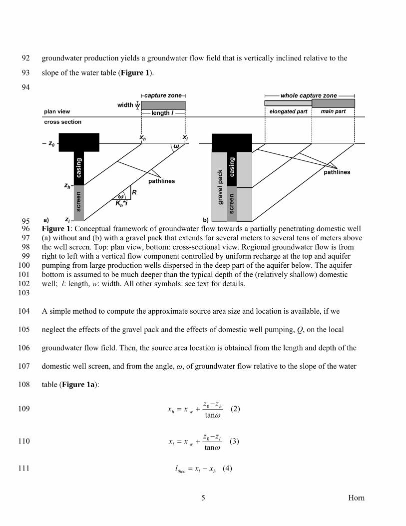
groundwater production yields a groundwater flow field that is vertically inclined relative to the 92

slope of the water table (Figure 1). 93

94

95 Figure 1: Conceptual framework of groundwater flow towards a partially penetrating domestic well 96 (a) without and (b) with a gravel pack that extends for several meters to several tens of meters above 97 the well screen. Top: plan view, bottom: cross-sectional view. Regional groundwater flow is from 98 right to left with a vertical flow component controlled by uniform recharge at the top and aquifer 99 pumping from large production wells dispersed in the deep part of the aquifer below. The aquifer 100 bottom is assumed to be much deeper than the typical depth of the (relatively shallow) domestic 101 well; l: length, w: width. All other symbols: see text for details. 102 103

A simple method to compute the approximate source area size and location is available, if we 104

neglect the effects of the gravel pack and the effects of domestic well pumping, Q, on the local 105

groundwater flow field. Then, the source area location is obtained from the length and depth of the 106

domestic well screen, and from the angle, ω, of groundwater flow relative to the slope of the water 107

table (Figure 1a): 108

ωtan0 h

whzz

xx−

+= (2) 109

ωtan0 l

wlzz

xx−

+= (3) 110

hltheo xxl −= (4) 111

Horn 6

RQAtheo /= (5) 112

theo

theotheo l

Aw = (6) 113

where xw is the location of the well (along the regional groundwater gradient), xh is the location of 114

the downgradient edge of the recharge (source) area, xl is the location of the updgradient edge of the 115

recharge area, z0 is the elevation of the water table, zh is the elevation of the top the well screen, zl is 116

the elevation of the bottom of the well screen (Figure 1a), ltheo, wtheo , Atheo are the theoretical length, 117

width, and area of the recharge zone, and: 118

tan ω = R / (Kh * i) (7) 119

where R is the uniform recharge rate, Kh is aquifer hydraulic conductivity, and i is the regional 120

hydraulic gradient. Equations (2) – (7) provide a simple analytical model to determine the capture 121

zone of a domestic well in an unconfined aquifer with uniform flow, recharge, and deep production. 122

123

To account for the influence of domestic well pumping on the local groundwater flow system around 124

the well and to account specifically for the influence of the gravel pack on the recharge area (Figure 125

1b), we constructed a numerical model, described in the next section. 126

127

Modeling Methods 128

The capture zone of a domestic well with a gravel pack is computed for a fully three-dimensional 129

steady-state groundwater flow field. The steady-state head and flux distribution are computed using 130

the MODFLOW groundwater flow model (McDonald and Harbaugh 1988). The capture zone 131

corresponding to a particular groundwater flow solution is delineated using the backward particle 132

tracking model MODPATH (Pollock 1994). 133

134

Horn 7

Briefly, MODFLOW solves the steady-state groundwater flow equation 135

0=∇∇ hK (8) 136

where h is the hydraulic head, by using a fully three-dimensional block-centered finite difference 137

scheme for the user-specified boundary conditions, K is the hydraulic conductivity tensor. In the 138

following simulations pumping induces only a small drawdown of the piezometric surface, so the 139

linear flow model (8) is sufficiently accurate for our purposes. We effectively invoke the Dupuit 140

assumption equivalent to the MODFLOW “unconfined layer” algorithm. There, the unconfined layer 141

thicknesses are set constant and only updated iteratively. From the hydraulic head solution, 142

MODFLOW also computes the flux, q, across each of the six faces of each finite difference cell in 143

the modeling domain. The flux solution becomes input to MODPATH, which computes backward 144

particle travel paths given the linear groundwater velocity, v = q/n, where n is the effective porosity, 145

across each finite difference cell face. Starting locations for backward particle paths are user-defined. 146

MODPATH uses a semi-analytical linear interpolation scheme to compute a spatially continuous 147

particle path (Pollock 1994). 148

Horn 8

149 150 Figure 2: Model grid in (a) cross-sectional view at y = 0 (Vertical exaggeration = 4.2x) and (b) in 151 plan view. Due to the symmetry of the flow field, the model domain simulates only half of a well 152 and half of the capture zone. The well and gravel pack are very finely discretized. A close-up view 153 of the model around the well screen is shown in Figure 4. 154 155

Our modeling domain is a finite difference grid with 141,750 cells of which 137,937 are active. The 156

modeling domain is 58 m high, 387.23 m long and 59.695 m wide and consists of 45 rows, 90 157

columns, and 35 layers. The modeling domain takes advantage of the symmetry in the well flow 158

field, which is symmetric across the x-axis (mean flow direction) centered on the domestic well (y = 159

0, see below). The model is therefore designed to model only one-half of the well capture zone 160

(Figure 2). The second half of the well-capture zone mirrors the first half. Grid spacing is non-161

Horn 9

uniform in both the vertical and horizontal direction. Vertical grid spacing varies from 1 m at the 162

elevation of the well screen to 4 m elsewhere (Figures 2, 3). Horizontal grid-spacing varies from 163

0.01 m near the well and in the gravel pack to nearly 20 m near the model boundaries. The 164

horizontal increase in cell-size between adjacent rows or columns of the finite-difference grid is set 165

to not exceed 50 % of its width. 166

167

The hydraulic gradient along the x-axis is produced by defining a constant head boundary of 58.00 168

m to the exterior block of cells at the upgradient vertical side of the model and a constant head of 169

57.61 m at the downgradient vertical side of the model (Figure 2). This is equivalent to a hydraulic 170

gradient of 0.0018, which is typical for the study area. The other two vertical planes of the model are 171

assigned no-flow boundary condition: the vertical plane adjacent to the well half is a symmetry 172

plane. The vertical plane opposite of the half well is at sufficient distance to the well that the local 173

effect of pumping on the groundwater flow field can be neglected and flow is parallel to regional 174

groundwater flow. The average (steady-state) recharge rate is set to 0.669 m/year, a value typical for 175

semi-arid, irrigated agricultural regions such as the Modesto Area, San Joaquin Valley, California. 176

The bottom of the model domain is considered permeable and open to the regional aquifer system 177

below. It is assigned a uniform constant (downward) flux boundary condition, with total outflow 178

across the bottom boundary set equal to the difference between the total recharge inflow at the top 179

and the well outflow rate. In this way we implicitly enhance our model to greater aquifer depths. In 180

the Modesto Area large irrigation wells up to a depth of almost 370 m below land surface pump 181

large amounts of water and produce a vertical flow component, even through a confining clay unit 182

above the irrigation wells (Burow et al. 2004). 183

184

Horn 10

The well construction was chosen to be representative of domestic well construction in the San 185

Joaquin Valley, California (e.g., Burow et al., 2004). The model well has a total depth of 56 m below 186

the water table. A seal to 18 m below the water table overlies a 30 m long gravel pack around a 187

blank well casing. The casing has a diameter of 0.2 m. The perforated well screen is located at 48 m 188

to 55 m below the water table, followed by a conceptual well sump from 55 m – 56 m. Casing and 189

screen are surrounded by a 0.09 m thick gravel pack. The total borehole diameter is 0.38 m. Due to 190

the relatively low pumping rate, the well-loss and skin effect are assumed to be negligible. Inflow 191

along the screen is computed by the model and non-uniformly distributed. 192

193

The grouted well seal above the gravel pack and the well casing are modeled as “no-flow” cells 194

(black cells in Figure 3). The pump is simulated by 74 “well” cells inside the casing. They are 195

located significantly above the top of the screen, opposite of the well seal bottom, which creates an 196

upward flow inside the screen and casing. The MODFLOW “well” package is used to simulate the 197

pump cells (light-grey cells in Figure 3). The total pumping rate of the domestic well is 3.5 m3/d, 198

half of which is uniformly distributed across the individual “well” cells at the top of the casing. 199

Flow inside the model well casing was modeled by approximating the flow with eq. (8) using very 200

high hydraulic conductivity. The gravel pack (grey cells in Figure 3) is modeled by choosing a 201

separate hydraulic conductivity that is higher than that of the surrounding aquifer and ranges 202

between 50 and 1000 [m/d] (Table 1). Modeling the pump inside the well allows the model to 203

properly distribute the flow across the well screen, with screen inflow highest near the top of the 204

screen and lowest at the bottom of the screen. 205

Horn 11

206 Figure 3: Model well configuration and grid discretization around the well. Left: Cross-section at 207 the model boundary (y = 0). Right: Plan view at the land surface (right top), at the top layer of the 208 casing containing the well cells (right center), and at the screen elevation (right bottom). Black cells: 209 casing and well seal (impermeable). Grey cells: gravel pack. Dark grey cells: constant flux boundary 210 cells at the model bottom. Grey dots in the lower left panel indicate the starting location for 211 backward particle tracking. 212 213

214

Horn 12

The hydraulic conductivity, Kh, is assumed to be isotropic in the horizontal plane, while the vertical 215

aquifer hydraulic conductivity, Kv, is lower, as typically observed in alluvial aquifers (e.g., Phillips 216

et al., 2007). Two representative anisotropy ratios, Kh/Kv = 5 and 2, were chosen to bracket a 217

representative range typically found in alluvial aquifers (ibid.). The gravel pack itself is assumed to 218

have a completely isotropic hydraulic conductivity, Kg, that is larger than Kh. For illustration and 219

application purposes, we modeled well capture zones for a wide range of representative values for 220

the horizontal hydraulic conductivity, Kh, and the gravel pack hydraulic conductivity, Kg, and for two 221

anisotropy ratios (Table 1). 222

Kh Kv Kg 1 0.2 50, 125, 250, 500, 750, 1000 1 0.5 50, 125, 250, 500, 750, 1000 3 0.6 50, 125, 250, 500, 750, 1000 3 1.5 50, 125, 250, 500, 750, 1000 5 1 50, 125, 250, 500, 750, 1000 5 2.5 50, 125, 250, 500, 750, 1000 10 2 50, 125, 250, 500, 750, 1000 10 5 50, 125, 250, 500, 750, 1000 30 6 50, 125, 250, 500, 750, 1000 30 15 50, 125, 250, 500, 750, 1000 100 20 125, 250, 500, 750, 1000 100 50 125, 250, 500, 750, 1000 300 60 500, 750, 1000 300 150 500, 750, 1000

223 Table 1: Model configurations with various 224 combinations of the horizontal hydraulic 225 conductivity, Kh, the vertical hydraulic 226 conductivity, Kv, and the gravel pack hydraulic 227 conductivity, Kg. All values are in units of 228 [m/d]. 229 230

Results 231

Head contour configurations in the aquifer around the domestic well are highly dependent on the 232

aquifer and gravel pack hydraulic conductivities. Cross-sectional head contour lines along the 233

Horn 13

regional flowpath are vertical under strictly regional flow with no recharge and no pumping. As 234

expected from the analytical model above, the modeled contours deviate from the vertical due to the 235

vertical flow component imposed by the recharge at the top of the model area and the regional 236

pumping below the modeled zone. Contour lines increasingly deviate from the vertical alignment 237

with smaller and smaller ratios of Kh / R (Figure 4). In addition, in aquifers with relatively low 238

hydraulic conductivity, the domestic well creates a distinct zone of local influence in the aquifer 239

around the well screen, whereas the influence is minimal in the highly permeable aquifer. The 240

anisotropy of the aquifer hydraulic conductivity creates significant flow zonation: much of the 241

impact of domestic well pumping on the pressure field is seen at the elevation of the well screens, 242

especially for those cases with the higher aquifer anisotropy. Another distinct horizontal zone is 243

created by the top of the gravel pack. The higher the gravel pack hydraulic conductivity (relative to 244

Kh), and the higher the aquifer anisotropy ratio, Kh/Kv, the more pronounced is the effect that the 245

transition between the top of the gravel pack and the annular seal has on the head contour lines (e.g., 246

Figure 4). Inflow to the well varies non-uniformly along the screen. It is highest near the top of the 247

screen, which is nearest to the pump intake inside the well-casing. The difference between the screen 248

inflow at the top (layer 26) and the screen inflow near the bottom (usually in layer 31 just above the 249

bottom of the layer) varies from approximately 45% for highly permeable aquifers to more than 250

100% for very low permeable aquifers with very high gravel pack Kg. This is consistent with 251

analytical models (Nahrgang, 1954; Garg and Lal, 1971) and with field observations on large 252

production wells (VonHofe and Helweg, 1998). 253

Horn 14

254 Figure 4: Head contour lines around the well for a conductivity of 10 m/d, an anisotropy ratio of 2, 255 and hydraulic gravel pack conductivity of 750 m/d. The heads depend on the conductivity of the 256 aquifer, the anisotropy and the relative difference in the conductivities between gravel pack and 257 aquifer. Horizontal dimension is 7 m, vertical dimension is 58 m. Due to the horizontal exaggeration 258 (12.4x) the inclination of the head contours in the regional flow field (near top of the cross-section 259 appears nearly horizontal although it is actually nearly vertical. 260 261

Corresponding to the head field, pathlines in low hydraulic conductivity aquifers are significantly 262

steeper and the capture zone is much closer to the well-head than in an aquifer with high hydraulic 263

conductivity (Figure 5). For Kh ≥ 10 m/day, the modeled pathlines are in fact sufficiently flat that 264

the source area is outside the model area. In those simulations, we computed the pathlines outside 265

the numerical modeling area by analytically calculating the extension of the pathlines to the water 266

table using equation (7). Also, for model scenarios with hydraulic conductivities of 1, 3, and 5 m/d, 267

the pathlines in the top aquifer layer were computed from eq. (7), because MODPATH computations 268

in the top layer were subject to numerical error. 269

Horn 15

270

The source area of the domestic well has a distinct shape composed of two features: the main 271

capture zone, a relatively large and wide oval area, corresponding to pathlines that enter the annulus 272

of the well below the top of the well-screen for horizontal delivery into the well. At the 273

downgradient (well-facing) side of this main capture zone, we observe a narrow elongated capture 274

subzone that represents those pathlines that enter the gravel-pack of the well at some distance above 275

the well screen. These pathlines capture domestic water through the high permeability field of the 276

gravel pack above the well screen (Figure 1b, Figure 5). The greater the hydraulic conductivity 277

difference between gravel pack and aquifer, the higher is the relative downward flow in the upper 278

gravel pack, and the more MODPATH virtual water particles enter the well flowing through the 279

upper gravel pack. Moreover, the steeper the particle path gradient, the higher is the highest point of 280

entry into the gravel pack of pathlines that ultimately will be captured by the well. Thus, the gravel 281

pack, where it extends to elevations much higher than the well-screen, significantly extends the 282

length of the source area towards the well, albeit within a very narrow transverse range (Figure 5). 283

284

Figure 5: Pathlines in cross section (left) and plan view (half the well, right) with the elongated and 285 main capture zone parts for an aquifer conductivity of 10 m/d, an anisotropy ratio of 2, and gravel 286 pack conductivity of 750 m/d. Corresponding heads are shown in Figure 4. 287

Horn 16

288

For further analysis of the capture zone location and size, we separately refer to the width and length 289

of the narrow, “elongated” part of the capture zone nearer to the well and of the “main” part of the 290

capture zone (Figure 6) from where the majority of the water originates. The simulations show that 291

the length of the elongated part increases faster than the length of the main part as horizontal aquifer 292

conductivity increases, but the gravel pack conductivity has a significant influence only on the 293

length of the elongated part (Figure 6c, d). The same is true for the width of the two capture zone 294

parts: The gravel pack conductivity has a significant influence only on the width of the elongated 295

part but little, yet discernable influence on the main part. The width of the elongated part increases 296

several-fold with gravel pack hydraulic conductivity, Kg, especially in less productive (low K) 297

aquifers. By the same token, the widths of the main and elongated parts (Figure 6a, b) decrease 298

with higher aquifer conductivities (more narrow, but longer source area). For low gravel pack 299

conductivities, the width of the elongated part of the capture zone remains nearly constant, 300

regardless of aquifer conductivity 301

Horn 17

302 Figure 6: Widths (top panels) and lengths (bottom panels) of the elongated part (right panels) and 303 the main part (left panels) of the capture zone for an anisotropy ratio of Kv: Kh = 1 : 2. Behavior of 304 the models with an anisotropy ratio Kv : Kh = 1 : 5 is similar. 305 306 The analytical model (eqs. 2,3) of the source area location provides good approximations of the 307

source area only in highly permeable aquifers. For aquifers with intermediate and low conductivity, 308

the gravel pack has significant influence on the distance of the downgradient edge of the capture 309

zone from the well (Figure 7a), where the source area can be as much as 90% closer to the well than 310

estimated from eq. 2. The analytical approximation of the distance from the well to the upgradient 311

edge of the source area (eq. 3) is relatively close to the numerical simulations if aquifer hydraulic 312

conductivities are above 5 m/d. In those cases, the relative difference between analytical and 313

numerical model is on the order of 10% or less (Figure 7b), regardless of anisotropy ratio and gravel 314

pack hydraulic conductivity. 315

Horn 18

316 Figure 7: Comparison of the distances of the source areas to the well provided by the numerical and 317 by the analytical model exemplarily for an anisotropy ratio of Kv: Kh = 1 : 2. (a) Normalized 318 differences between the modeled and analytically calculated distances of the downgradient edges of 319 the source areas to the well. (b) Normalized differences of the distances of the upgradient edges of 320 the source areas to the well. 321 322

The simulation results show that water moves downward inside the gravel pack above the well-323

screen from considerable distances: For Kh less than 10 m/d and high gravel pack hydraulic 324

conductivities, water travels downward from as far as the top of the gravel pack, 30 m above the 325

well-screen (Figure 8). Again, the more permeable the gravel pack in the annulus, the larger the 326

above-screen capture of source water. The fraction of well pumpage that originates from capture in 327

the gravel pack above the well-screen increases as the aquifer hydraulic conductivity decreases 328

(Figure 9). In intermediate and low permeable aquifers, domestic wells with highly permeable 329

gravel packs receive from 20% to 50% of the total well flow from the extended gravel pack above 330

the screened aquifer horizon. This model result is qualitatively consistent with the field data of 331

Houben (2006), who found iron oxide incrustations in the gravel pack significantly above the top of 332

the well screen, where the incrustations were due to a significant amount of water flowing through 333

the upper part of the gravel pack. At high aquifer conductivities (Kh > 10 m/d), less than 12 % of the 334

Horn 19

total domestic well flow originate from the gravel pack above the well screen. Aquifer anisotropy 335

has little influence on the height of the capture zone within the gravel pack. 336

337

The height of the gravel pack participating in flow to the well and the percent fraction of the 338

pumpage originating from the gravel pack above the screen can be expressed quantitatively: Table 339

2 provides the regression coefficients obtained by fitting data in Figures 8a and 8b to nonlinear 340

exponential regression equations of the form: 341

y = a*exp(-log(Kh)/b) (9) 342

using the Levenberg-Marquardt algorithm for optimization. For application to a specific site, linear 343

interpolation of the values for a and b in Table 2 may be used to compute the height of capture in 344

the gravel pack and the proportion of flow originating from the gravel pack above the well screen for 345

values of the anisotropy ratio and of Kg other than those given in the Table. This modified analytical 346

tool provides a much more realistic source area than the much simpler graphical method employed 347

in many states as part of their source water assessment programs (e.g., California DHS 1999). 348

Horn 20

349

Figure 8: (a) Maximum virtual water particle heights in the gravel pack above the well screen 350 serving to capture water (b) Percentage of inflow into the well screen flowing through the gravel 351 pack from above the screen. Both for an anisotropy ratio of 2. 352 353 354 355 356

Parameter for maximum heights:

Parameter for inflow from above:

Anisotropy

Kg

a b

Adjusted r2

A b

Adjusted r2

2 50 33.31 1.05 1.00 12.69 0.60 0.99 2 125 77.01 0.88 0.99 21.44 0.69 0.99 2 250 87.95 1.02 1.00 30.59 0.76 0.99 2 500 163.35 0.93 1.00 40.57 0.86 0.99 2 750 172.04 1.00 1.00 47.16 0.92 0.99 2 1000 226.70 0.96 0.94 52.10 0.96 0.98 5 50 79.01 0.78 0.95 14.94 0.61 1.00 5 125 98.28 0.93 0.97 25.14 0.70 0.99 5 250 216.33 0.80 0.93 35.57 0.77 0.99 5 500 276.67 0.87 0.99 47.59 0.85 0.99 5 750 396.12 0.85 0.99 55.54 0.91 0.99 5 1000 401.91 0.88 1.00 61.39 0.96 0.98 Table 2: Coefficients and adjusted coefficients of determination (r2) for the equations describing the 357 maximum heights of the capture zone in the gravel pack, and the inflow of water entering the well 358 from the gravel pack above the screen. 359 360 361 362

Horn 21

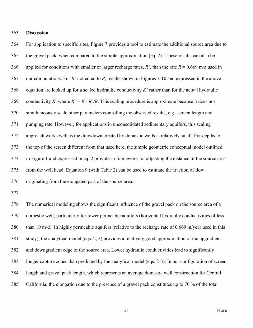
Discussion 363

For application to specific sites, Figure 7 provides a tool to estimate the additional source area due to 364

the gravel pack, when compared to the simple approximation (eq. 2). These results can also be 365

applied for conditions with smaller or larger recharge rates, R’, than the rate R = 0.669 m/a used in 366

our computations. For R’ not equal to R, results shown in Figures 7-10 and expressed in the above 367

equation are looked up for a scaled hydraulic conductivity K’ rather than for the actual hydraulic 368

conductivity K, where K’ = K · R’/R. This scaling procedure is approximate because it does not 369

simultaneously scale other parameters controlling the observed results, e.g., screen length and 370

pumping rate. However, for applications in unconsolidated sedimentary aquifers, this scaling 371

approach works well as the drawdown created by domestic wells is relatively small. For depths to 372

the top of the screen different from that used here, the simple geometric conceptual model outlined 373

in Figure 1 and expressed in eq. 2 provides a framework for adjusting the distance of the source area 374

from the well head. Equation 9 (with Table 2) can be used to estimate the fraction of flow 375

originating from the elongated part of the source area. 376

377

The numerical modeling shows the significant influence of the gravel pack on the source area of a 378

domestic well, particularly for lower permeable aquifers (horizontal hydraulic conductivities of less 379

than 10 m/d). In highly permeable aquifers (relative to the recharge rate of 0.669 m/year used in this 380

study), the analytical model (eqs. 2, 3) provides a relatively good approximation of the upgradient 381

and downgradient edge of the source area. Lower hydraulic conductivities lead to significantly 382

longer capture zones than predicted by the analytical model (eqs. 2-3). In our configuration of screen 383

length and gravel pack length, which represents an average domestic well construction for Central 384

California, the elongation due to the presence of a gravel pack constitutes up to 70 % of the total 385

Horn 22

length of the capture zone. The elongation is relatively narrow but higher gravel pack conductivities 386

lead to significant increases in that width. The width of the main capture zone, in turn, slightly 387

decreases at higher gravel pack conductivities. The greater the difference between hydraulic 388

conductivity of the aquifer and that of the gravel pack, the greater is the elongated part relative to the 389

total length of the capture zone. 390

391

For many contaminants, chemical or microbial, aquifer attenuation is a dynamic, time-dependent 392

process. Travel times for potential contaminants decrease approximately linearly with increased 393

gravel pack length above the well screen. This is due to the strong influence of recharge on vertical 394

downward displacement of water (and contaminants) and the relatively small influence that the 395

domestic well pumping exerts on the overall groundwater flow field. A linear decrease in travel time 396

from the time of recharge until arrival at the gravel pack is associated with exponentially increased 397

contaminant concentrations. The gravel pack itself typically provides much less attenuation capacity 398

than the aquifer material. Hence, a short seal and vertically extended gravel pack constitute a 399

potential short-circuit for contaminants. 400

401

We also note that the fraction of flow captured by the gravel pack above the well screen may be 402

relatively small in a productive (high K) aquifer. But for some contaminants the resulting dilution 403

with (good) groundwater collected by the well at the depth of the screen may not be sufficient. This 404

includes contaminants that reach the water table at concentrations that are several orders of 405

magnitude above regulatory drinking water limits including solvents, pesticides, other organic 406

chemicals, and pathogens. A possibly common source of such contamination are septic tank leach 407

Horn 23

fields, which - in rural and semi-rural housing developments - are often located in the vicinity of 408

domestic wells. 409

410

Conclusions 411

Our work provides a tool to quickly estimate the size and location of the source area of domestic 412

wells in regions with significant recharge (for example, due to irrigation). The influence of the 413

gravel (or sand) pack in the well annulus above the well screen is explicitly accounted for. Results 414

allow for estimation of source area and gravel pack impact for a wide range of scenarios. 415

Importantly, we show that the gravel pack above the well screen poses a significantly increased risk 416

for domestic well contamination. A gravel pack that extends significantly above the well screen (due 417

to short seal length), may significantly enhance the length of the source area, thus exposing the well 418

to a larger cross-section of potential contaminant sources. The extended gravel pack also decreases 419

travel time and distance for contaminants from the source area to the well allowing for contaminants 420

to partially circumvent natural aquifer attenuation. This is especially true in aquifers with low to 421

intermediate hydraulic conductivity (K ≤ 10 m/d). We therefore strongly recommend that the gravel 422

(or sand) pack not be extended more than a few meters above the well screen of a domestic well. 423

424

Acknowledgments. We gratefully acknowledge the careful review and constructive comments of 425

Karen Burow, USGS, and two anonymous reviewers. Funding for this research was provided 426

through a fellowship of the German Academic Exchange Service (DAAD) to Judith Horn. 427

428

429

430

Horn 24

References 431

Belitz, K., and S. P. Phillips (1995), Alternative to agriculture drains in California’s San Joanquin 432 valley: results of a regional-scale hydrogeologic approach, Water Resour. Res., 31(8), 1845-1862. 433 434 Burow, K. R., J. L. Shelton, J. A. Hevesi, and G. S. Weissmann. 2004. Hydrogeologic 435 characterization of the Modesto area, San Joaquin Valley, California. USGS Scientific Investigations 436 Report 2004-5232. 437 438 California DHS. 1999. Drinking Water Source Assessment and Protection (DWSAP) Program. 439 Division of Drinking Water and Environmental Management, California Department of Health 440 Services. Sacramento, CA. http://www.dhs.ca.gov/ps/ddwem/dwsap/DWSAPindex.htm 441 442 Garg, S. P. and J. Lal, 1971. Rational design of well screens. J. Irrig. and Drain. Div., ASCE, 443 97(1):24-35. 444 445 Harter, T. 2008. Delineation of wellhead protection areas. In: T. Harter and L. Rollins (eds.), 2008. 446 Watersheds, Groundwater, and Drinking Water: A Practical Guide, University of California, UC 447 ANR Communications Services Publication 3497, Davis, CA 95616, 274p. 448 449 Houben, G. H. 2006. The influence of well hydraulics on the spatial distribution of well 450 incrustations. Ground Water 44, no. 4: 668-675. 451 452 McCray, J. E., S. L. Kirkland, R. L. Siegrist, and G. D. Thyne. 2005. Model parameters for 453 simulating fate and transport of on-site wastewater nutrients. Ground Water 43, no. 4: 628-629. 454 455 McDonald, M. G. and A. W. Harbaugh. 1988. Technics of water-resources investigation of the 456 United States Geological Survey. USGS Open-File Report 83-875. 457 458 Nahrgang, G., 1954. Zur Theorie des vollkommenen und unvollkommenen Brunnens. 43 p. 459 460 Phillips, S. P., C. T. Green, K. R. Burow, J. L. Shelton, and D. L. Rewis, 2007. Simulation of 461 ground-water flow in part of the Northeastern San Joaquin Valley, California, U.S. Geological 462 Survey, Scientific Investigations Report, SIR 2007-5009. 463 464 Pollock, D. W. 1994. User’s guide for MODPATH/MODPATH-PLOT, Version 3: A particle 465 tracking post-processing package for MODFLOW, the U. S. Geological Survey finite-difference 466 ground-water flow model. USGS Open-File Report 94-464. 467 468 Todd, D. K. 1980. Ground water hydrology, 2nd ed. New York: John Wiley and Sons. 469 470 U.S. EPA. 1997. Response to Congress on use of decentralized wastewater treatment systems. 471 Washington, D.C.: Office of Water, U.S. EPA. 472 473 VonHofe, F. and O. J. Helweg, 1998. Modeling well hydrodynamics. ASCE J. Hydr. Eng. 474 124(12):1198-1202. 475

Horn 25

476