Production patterns of Multinational Firms: Horizontal and Vertical Multinationals with traded intermediates1

Kazuhiko OYAMADA and Yoko UCHIDA

1. Introduction

One of the key factors behind the growth of global trade in recent decades is an increase

in intermediate input as a result of the development of vertical production networks

(Feensta, 1998). Manufacturing goods are no longer produced in a single country.

Production processes are subdivided into several stages, in which respective countries

specialize in producing parts and components. Many countries are involved in vertical

production networks of producing just a single final good for consumers.

It is widely recognized that the production networks have formed due to the

expansion of multinational enterprises’ (MNEs) activities. Multinational enterprises

have been differentiated into two types according to their production structure:

horizontal FDI and vertical FDI. However, a new type of FDI which diverges from the

vertical one has been proposed in the context of the recent expansion of more complex

multinational activities; it is called export-platform FDI. Horizontal FDI maintain

affiliates in home and host countries with the headquarters located in the home country,

while vertical and export-platform FDI install affiliates in host countries with the

headquarters located in the home country. The difference between vertical and export-

platform FDI is where their products are sold: vertical FDI seek to sell their products in

both the home and host country, while export-platform FDI seek to sell in a third market

through the affiliates in the host country (Ekholm et al., 2007 and Matsuura and

1 This paper is modified version of IDE Discussion Paper Series No. 290

1

Hayakawa, 2008).

Theoretical research on MNEs has been conducted since the early 1960s

(Hymer, 1976), but it developed dramatically from the mid 1980s as a result of the

“new” trade theory. There are two important theoretical models of MNEs: one was

presented by Helpman (1984) and the other by Markusen (1984). Helpman’s model

treats vertical MNEs with monopolistic competition and without trade costs. On the

other hand, Markusen’s model treats horizontal MNEs with one factor, assuming firm-

level scale economy. Markusen (1997) combines horizontal and vertical motives in a

model, so the model allows two types of MNE to exist at the same time. This is called

the “knowledge capital” model. Zhang and Markusen (1999) extended the model to

consider vertical MNEs that supply intermediate inputs to a final production plant in a

host country. While their models were constructed in a two-region framework, Ekholm

et al. (2007) extended the model into a three-region framework to include export-

platform FDI. Ekholm et al. (2007) and other models such as Yeaple (2003) and

Grossman et al (2006) in the three-regional framework assume that skilled-labor-

intensive intermediates are produced only at home, and the host country imports

intermediate products and assembles final goods, combining intermediates and unskilled

labor. However, those models do not adequately explain observed facts where some

kinds of intermediate goods are produced in the host country.

After Ekholm et al.(2007), a series of Markusen type models have not been

fully developed because main stream of MNE studies have shifted to Melitz type model

in which firm heterogeneity are taking into consideration since Melitz (2003). A series

of Melitz type models, such as Helpman et al. (2004) and Graossman et al. (2006)

analyze change of firm’s exporting activities and FDI activities by incorporating firm

2

heterogeneity and fixed cost related to exports in Krugman’s imperfect competition

model (1980). In those models, each firm’s productivity level is endogenously

determined under certain amount of fixed cost. On the other hand, Markusen type model

analyze firm type by changing fixed cost under certain level of firm’s productivity. In

this regards, Melitz type model and Markusen type model can be regarded as two sides

of the same coins. Since each type of model has strengthen and weakness, it is

important to use both types of model in order to clarify the condition of FDI. Although

Melitz type models have been fully accumulated recently, Markusen type model have

not.

Ekholm et al. (2007) and other models in the three-regional framework assume

that skilled-labor-intensive intermediates are produced only at home, and the host

country imports intermediate products and assembles final goods, combining

intermediates and unskilled labor. However, those models do not adequately explain

observed facts where some kinds of intermediate goods are produced in the host

country.

Our final goal is to extend Ekholm et al. (2007) to treat the procurement of

intermediates from the host country in view of the present situation. We start from the

simple model in the two-region framework in preparation for further extension. In this

paper, we extend Zhang and Markusen (1999) to include horizontal and vertical FDI in

the model with traded intermediates. There are no studies which treat vertical and

horizontal FDI with traded intermediates at once, although more evolved models which

treat vertical, horizontal and export-platform FDI with traded intermediates, such as

3

Ekholm et al. (2007), do exist. This paper serves to bridge the gap between Zhang and

Markusen (1999) and Ekholm et al. (2007) in theoretical studies of FDI.

The remainder of this paper is organized as follows. The next section

introduces the assumptions of the model and model structure. Section three provides the

numerical general equilibrium model, then section four presents the simulation results.

Finally, our conclusions and future extension are presented in section five.

2. The Model

2.1 Assumptions of the Model

The following three assumptions are borrowed from Markusen (2002:129):

1. Fragmentation: the location of knowledge based assets may be fragmented from

production. Any incremental cost of supplying services of the asset to a single

foreign plant versus the cost to a single domestic plant is small.

2. Skilled-labor intensity: knowledge-based assets are skilled labor intensive relative

to final production.

3. Jointness: the services of knowledge based assets are (at least partially) joint

(“public”) inputs into multiple production facilities. The added cost of a second

plant is small compared to the cost of establishing a firm with local plant.

Fragmentation and skilled-labor intensity motivate vertical MNEs, while jointness is

4

associated with horizontal MNEs. It should be noted that fragmentation and jointness

are not the same thing. Fragmentation can be interpreted as service provided by skilled

labor, such as manager service. Manager skill can be transferred easily by shifting a

manager from home to host, but cannot be simultaneously used in both because a

manager can only be in one place at any one time. On the other hand, jointness, which

can be represented by a blueprint, can easily be shared among plants without reducing

the services provided in other locations.

2.2 Model Structure

There are two identical countries, denoted by i and j, producing two final goods using

two factors, unskilled labor L and skilled labor S. L and S are required in both sectors

and are mobile between sectors, but are internationally immobile.

Y is produced with L and S using a Cobb-Douglas type constant return to scale

technology and under perfect competition. Y will be used as numeraire and so its price

is set to unity. The production function for Y is:

Y i=(S iY )α ( Li

Y )1−α, (1)

where SiY

and LiY

are skilled and unskilled labor used in the Y sector in country i.

Subscripts i and j will respectively be used to denote countries 1 and 2. Marginal

products of S and L in Y production are:

5

piS=α ( Si

Y

LiY )

α−1 and pi

L= (1−α )( S iY

LiY )

α, (2)

where piS and pi

L are wages for skilled and unskilled labor, respectively.

Good X is produced with increasing returns to scale technology by imperfectly

competitive Cournot firms. X is produced in two stages. In the first stage, the

intermediate product M is produced only in country i using skilled labor S alone. In the

second stage, X is assembled using unskilled labor and intermediate inputs M. There are

both firm-level and plant-level scale economies. There are free entry and exit of the

firms, and entering firms choose their “type.” There are six firm types, which are

defined as follows:

Type di: National firms that maintain a single plant, with headquarters in country i.

Type-di firms produce M and X in country i. Some X may or may not be

exported to country j.

Type hi: Horizontal MNEs that maintain plants in both countries, with headquarters

located in country i. Type-hi firms produce M in country i, some of which is

shipped to an assembly plant in country j. X is produced in both countries.

Some of X may or may not be exported to country i.

Type vi: Vertical MNEs that maintain a single plant, with headquarters in country i.

Type-vi firms produce M in country i, which is then shipped to an assembly

plant in country j. Some X may or may not be exported to country i.

Figure 1 shows an image of each type of firm in the case when i = 1. In each

6

pattern, the headquarters of the firm is located in country 1.

Figure 1: Firm type

type-di firm type-hi firm type-vi firm

HQ HQ HQ

AssemblyPlant

AssemblyPlant

AssemblyPlant

AssemblyPlant

Market 1 Market 2 Market 1 Market 2 Market 1 Market 2

X11

M11

X12 X21 X22

M12

X11

M11

X22

M12

The model allows domestic and multinational firms to arise endogenously. The term

“regime” will denote the set of firm types active in an equilibrium.

There are additional assumptions regarding factor-intensity from the view

points of activities and firm types. The factor-intensity assumption in terms of activities

is as follows:

[headquarters only] > [integrated X] > [plant only] > [Y].

In terms of firm types, the assumption is:

[type-h firms] > [type-v and type-d firms].

Superscripts (k = d, v, h) will be used to designate a variable as referring to

domestic firms, vertical MNEs, and horizontal MNEs, respectively. N ik will indicate the

number of type-k firms active in an equilibrium in country i. The cost structure of

industry X is as follows:

7

θS Unit input requirement for factor S

θL Unit input requirement for factor L

θM Unit input requirement for intermediate input M

τ X Units of L required to ship one unit of X. This is paid by the exporting country.

τ M Units of L required to ship one unit of M. This is paid by the exporting country.

G Plant-specific fixed cost in units of L required for the fixed costs of an X

assembly plant, incurred in country i for type-d firms and type-h firms. Also, in

country j for type-h and type-v firms, G is the same for any plant regardless of

the type of firm and country.

F Firm-specific fixed cost in units of S required for the fixed costs of an X

assembly plant, incurred in country i regardless of the firm type, and in country

j for type-h and type-v firms. F ij (i= j)k will be the skilled-labor requirement in the

home or parent country, while F ij (i ≠ j )k will be the skilled-labor requirement in

the foreign or host country.

Markusen (2002:135) makes three other assumptions regarding fixed cost as

follows. First, he assumes that skilled-labor requirements for a type-h firm are greater

than (but less than double) the skilled-labor requirements of a type-d firm. This is the

jointness assumption. Second, the additional skilled-labor requirements of a type-h firm

over a type-d firm are incurred partly in the home country and partly in the host country.

The last assumption is that managerial and coordination activities require some

additional skilled labor in the parent country for a type-h firm. For a firm based in

country i, the following relationship exists:

8

Jointness: 2 Fij (i= j )d >∑

jFij

h>F ij (i= j)d and F ij (i= j)

h >F ij ( i= j)d .

Fragmentation is not perfect in that some costs are incurred in order to transfer

technology. Therefore, type-v firms have higher skilled-labor requirements than type-d

firms, but less than type-h firms:

Fragmentation: ∑j

F ijh>∑

jFij

v>Fij (i= j)d .

A specific example used in our numerical model is described below. The

values are:

G=2, F ij (i= j)d =11, F ij (i= j)

h =12 and F ij (i ≠ j )h =4, F ij (i= j)

v =9 and F ij (i ≠ j )v =3.

Total fixed cost requirements for firms are:

type-d1 type-h1 type-v1 type-d2 type-h2 type-v2L 1 2 2 -- -- 2 --S 1 11 12 9 -- 4 3L 2 -- 2 2 2 2 2S 2 -- 4 3 11 12 9

The total fixed costs of type-d, type-h and type-v are 13, 20 and 14, respectively.

Next, the production costs of each type of firm are introduced.

Type-d firms

9

Type-d firms produce three products: X ij (i= j)d , X ij (i ≠ j )

d , and M ij ( i= j )d . The skilled-labor

requirements for type-d firms in country i are given by:

Sij (i= j )d =F ij (i= j)

d +θS M ij (i= j)d and M ij ( i= j )

d =θM∑j

X ijd. (3)

The unskilled-labor requirements in country i are:

Lij (i= j )d =G+θL∑

jX ij

d +τ X X ij ( i≠ j )d . (4)

Therefore, the cost function of type-d firms is given by:

piS Sij (i= j)

d +p iL Lij (i= j )

d

¿ ( piSθS θM+ p i

LθL) X ij ( i= j )d + {p i

S θSθM+ piL (θL+τ X )} X ij (i ≠ j )

d

+( p i

S Fij (i= j)d + pi

L G ). (5)

Type-h firms

Type-h firms produce four products: X ij (i= j)h , X ij (i ≠ j )

h , M ij ( i= j )h , and M ij ( i ≠ j )

h . The

skilled-labor requirements for type-h firms in country i are given by:

Sij (i= j )h =F ij (i= j)

h +θS∑j

Mijh and M ij

h=θM X ijh. (6)

The unskilled-labor requirements in country i are:

10

Lij (i= j )h =G+θL X ij (i= j )

h + τ M M ij ( i ≠ j )h . (7)

The skilled-labor requirements in country j are:

Sij (i ≠ j)h =F ij (i ≠ j )

h . (8)

The unskilled-labor requirements in country j are:

Lij (i ≠ j)h =G+θL X ij (i ≠ j)

h . (9)

Therefore, the cost function of type-h firms is given by:

∑j

( p jS Sij

h+ p jL Lij

h )

¿ ( piSθS θM+ p i

LθL) X ij ( i= j )h + {( pi

SθS+ piL τ M )θM+ p j

L θL} X i j (i ≠ j )h

+∑j

( p jS Fij

h + p jLG ). (10)

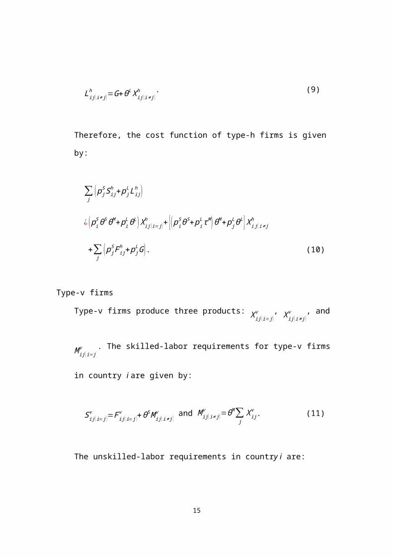
Type-v firms

Type-v firms produce three products: X ij (i= j)v , X ij (i ≠ j )

v , and M ij ( i= j )v . The skilled-labor

requirements for type-v firms in country i are given by:

Sij (i= j )v =F ij (i= j)

v +θS M ij (i ≠ j)v and M ij ( i ≠ j )

v =θM∑j

X ijv . (11)

11

The unskilled-labor requirements in country i are:

Lij (i= j )v =τ M M ij (i ≠ j)

v . (12)

The skilled-labor requirements in country j are:

Sij (i ≠ j)v =F ij (i ≠ j )

v . (13)

The unskilled-labor requirements in country j are:

Lij (i ≠ j)v =G+θL∑

jX ij

v+τ X X ij (i= j )v . (14)

Therefore, the cost function of type-v firms is given by:

∑j

( p jS Sij

v+ p jL Lij

v )

¿ {( piS θS+ pi

L τM )θM+ p jL (θL+ τX )} X ij ( i= j )

v

+{( piSθS+ pi

L τ M )θM+ p jL θL} X ij ( i≠ j )

v +∑j

( p jS F ij

v+ p jL G ). (15)

Let Si and Li denote total factor endowments in country i. The factor market

equilibrium can be defined by:

Si=S iY+N i

d Sij (i= j)d +∑

j(N j

h S jih +N j

v S jiv ), (16)

12

Li=LiY +N i

d Lij ( i= j )d +∑

j( N j

h L jih +N j

v L jiv ). (17)

In an equilibrium, the X sector makes no profit, so country i’s national income

denoted by Qi is:

Qi=piS S i+ p i

L Li. (18)

Let X iC and Y i

C denote the consumptions of X and Y in country i. The utility of a

representative consumer in each country is assumed to be defined by the following

Cobb-Douglas type function:

U i=( X iC )β (Y i

C)1−β (19)

where,

X iC=∑

j(N j

d X jid +N j

h X jih +N j

v X jiv ) and Y i

C=Y i.

Maximizing utility subject to the income constraint, we obtain the first-order conditions

that give demands for X and Y:

piX X i

C=β Qi and Y iC= (1−β )Qi (20)

13

An equilibrium in the X sector is determined by the pricing equation (marginal

revenue equals marginal cost) and free entry conditions. The proportional markup of

price over marginal cost is denoted by ε ijk. This can be read as the markup of a type-k

firm in country j. The pricing equations of each type of firm are:

piX (1−εij (i= j)

d )≤ p iS θS θM+ pi

L θL, (21)

piX (1−ε ij (i ≠ j )

d )≤ piS θS θM + pi

L (θL+ τ X ), (22)

piX (1−εij (i= j)

h )≤ p iS θS θM+ pi

L θL, (23)

piX (1−ε ij (i ≠ j )

h )≤ piS θS θM + pi

L τ M θM+ p jL θL, (24)

piX (1−εij (i= j)

v )≤ p iS θS θM+ pi

L τ M θM + p jL ( θL+τ X ), (25)

piX (1−ε ij (i ≠ j )

v )≤ piS θS θM + pi

L τ M θM+ p jL θL. (26)

The optimal markup in a Cournot model with homogenous products is given by the

firm’s share divided by the Marshallian price elasticity of demand in that market. Since

Marshallian elasticity of demand is −1 in this model with Cobb-Douglas demand, a

firm’s markup can be rewritten as:

14

ε ijk=

p jX X ij

k

β Q j

. (27)

Substituting the markup equations shown above into the pricing equations gives the

following expressions for demand or output in terms of price:

X ij (i= j)d ≥ β Qi[ pi

X−piS θSθM−p i

L θL

( piX )2 ], (28)

X ij (i ≠ j )d ≥ β Q j [ p j

X−p iS θS θM−pi

L (θL+ τ X )

( p jX )2 ], (29)

X ij (i= j)h ≥ β Qi[ pi

X−piS θSθM−p i

L θL

( piX )2 ], (30)

X ij (i ≠ j )h ≥ β Q j [ p j

X−p iS θS θM−pi

Lτ M θM−p jL θL

( p jX )2 ],

(31)

X ij (i= j)v ≥ β Qi[ pi

X−piS θSθM−p i

L τM θM−p jL ( θL+τ X )

( p iX )2 ], (32)

15

X ij (i ≠ j )v ≥ β Q j [ p j

X−p iS θS θM−pi

Lτ M θM−p jL θL

( p jX )2 ].

(33)

There are three zero profit conditions, corresponding to the three types of

firms. Zero profit conditions can be given as the requirement that markup revenues are

less than or equal to fixed costs:

∑j

p jX εij

d X ijd ≤ pi

S F ij (i= j )h + p i

L G, (34)

∑j

p jX εij

h X ijh ≤∑

j( p j

S F ijh+ p j

L G ), (35)

∑j

p jX εij

v X ijv ≤∑

jp j

S Fijv+ p j

L G. (36)

Using equations (28) through (33), the zero profit conditions (34) through (36) can be

rewritten as:

( piX−pi

SθS θM−piL θL ) X ij (i= j )

d

+ {p jX−p i

S θS θM− piL (θL+ τX )} X ij ( i≠ j )

d

≤ p iS Fij (i= j)

h + piL G, (37)

16

( piX−pi

SθS θM−piL θL ) X ij (i= j )

h

+( p jX−pi

S θS θM−piLτ M θM−p j

L θL) X i j (i ≠ j)h

≤∑j

( p jS F ij

h+ p jLG ), (38)

{ p iX−pi

SθS θM−piL τ M θM−p j

L (θL+τ X ) } X ij (i= j )v

+( p jX−pi

S θS θM−piLτ M θM−p j

L θL) X ij ( i≠ j )v

≤∑j

p jS Fij

v+ p jL G. (39)

To summarize the X sector in the model, the twelve inequalities (28) through

(33) are associated with the twelve output levels, and the six inequalities (37) through

(39) are associated with the number of firms in each regime. Factor prices can be

derived from factor-market-clearing conditions (16) and (17). Goods prices are obtained

by equation (20).

3. The Numerical General Equilibrium Model

Markusen (2002) pointed out two difficulties in solving the model by comparative

statics: one difficulty is the “many dimensions of the model” and the other is the “many

inequalities of the model”. In this paper, we formulate the model as a complementarily

problem following Markusen (2002). The program code for the general algebraic

17

modeling system (GAMS) is given in the Appendix2.

Table 1 shows the value used in the calibration of our model to the center of the

Edgeworth box, where only type-h firms are active due to the high trade cost of 20%.

Viewed in the column-wise direction, the table shows the input structure, while viewed

in the row-wise direction, the table shows the output distributions. A zero column sum

implies that the zero profit conditions are satisfied and a zero row sum indicates that the

market-clearing conditions are satisfied. Positive entries are receipts, while negative

entries are payments. All activity levels are one initially, except type-h activities. There

are five type-h firms (2.5 for each type-h firm) at the initial point, so the markup is 20%.

The fixed costs of other firm types are defined earlier in this paper. θS, θL and θM are

exogenously determined as 1.0, 0.875 and 0.125.

Table 1 Calibration of the model at the center of the Edgeworth boxY1 Y2 X11 X12 X22 X21 N1 N2 U1 U2 CONS1 CONS2 ENT1 ENT2 Rowsum

CY1 100 -100 0CY2 100 -100 0CX1 50 50 -100 0CX2 50 50 -100 0FC1 20 -20 0FC2 20 -20 0L1 -80 -35 -35 -2 -2 154 0S1 -20 -5 -5 -12 -4 46 0L2 -35 -35 -2 -2 154 0S2 -5 -5 -4 -12 46 0UTIL1 200 -200 0UTIL2 200 -200 0MK11 -10 10 0MK12 -10 10 0MK22 -10 10 0MK21 -10 10 0Colsum 0 0 0 0 0 0 0 0 0 0 0 0 0 0

CY Price of good Y Y Output of YCX Consumer price of X X Output of X by type-h firmFC Price of fixed cost N Output of fixed cost for type-h firmL Price of unskilled-labor U WelfareS Price of skilled-labor CONS Income of representative consumer UTIL Price of a unit of utility ENT Income of the owner of type-h firmsMK MarkupSource : Markusen (2002), Multinational Firms and the Theory of International Trade , Massachusetts : MIT press, p. 161.

2 Note that some solutions might not be found when one runs the presented program, which solves the model 361 times. Such kind of error occurs when the choice of initial values of variables becomes inadequate under certain conditions. One may solve the model individually by setting other initial values to recover the lost solutions.

18

The elasticity of substitution Y is derived by calibration of the model, using the

values in Table 1.

4. Simulation Results

Figures 2-5 present world Edgeworth boxes, where the vertical dimension is the total

world endowment of S (skilled-labor) and the horizontal axis is the total world

endowment of L (unskilled-labor). In the Edgeworth boxes, division of the world factor

endowment between two countries is shown with country 1 measured from the

southwest (SW) corner and country 2 measured from the northeast (NE) corner. The

model is repeatedly solved for each cell 361 times, altering the distribution of factor

endowments. Each cell of Figures 2-5 represents the equilibrium regime and the

numbers inside the cell show which type of firm is active in the regime. Table 2

presents the values we used to show which type of firm is active. For example, if the

value in the cell is 101, it shows that the domestic and horizontal firms of country 1 are

active. Also, number 110.01 shows that the domestic and vertical firms of country 1 and

domestic firms of country 2 are active. Figures 2-5 are gradation-coded according to the

active firm type.

Table 2 Values for the firm type

Country 1 Country 2Domestic 100 10Horizontal 1 0.1Vertical 0.01 0.001

Figure 2 shows the equilibrium regime at 20% transportation cost of final good

19

X and 20% of intermediate input M. This is the base case of our simulation analyses.

The values shown in Table 1 are used to solve the model at the center of the Edgeworth

box. The figure is read as follows: The center of the Edgeworth box, where countries

are similar in size and in relative endowment, shows there are only type-h firms. The

number 0.01 at the top-left corner of the figure means that there are only type-v1 firms,

where 95% of world skilled-labor endowment and 5% unskilled-labor endowment are in

country 1. At the edges of the box are the regions in which only type-v firms are active

in each equilibrium. This means that type-v firms are active when countries differ in

relative factor endowment.

Figure 2 Equilibrium regime in the base case (τ X=0.2 , τ M=0.2)O2

0.95 0.010 0.010 0.010 0.010 0.010 0.010 0.010 0.010 0.010 100.010 100.010 100.010 100.010 100.010 100.010 100.010 100.010 100.000 MLY0.90 0.010 0.010 0.010 0.010 0.010 0.010 0.010 0.010 100.010 100.010 101.01 101.01 101.010 101.010 101.010 101.010 100.000 100.000 100.001

0.85 0.010 0.010 0.010 0.010 0.010 0.010 0.010 100.010 101.010 101.010 101.010 101.010 101.010 101.000 101.000 101.000 100.000 100.001 100.001

0.80 0.010 0.010 0.010 0.010 0.010 0.010 101.010 101.010 101.010 101.010 101.010 101.000 101.000 101.000 101.000 100.000 100.001 100.001 100.001

0.75 0.010 0.010 0.010 0.010 0.010 1.010 1.010 1.010 1.010 1.000 1.000 101.000 101.000 101.000 100.100 100.100 100.001 100.001 100.001

0.70 0.010 0.010 0.010 0.010 1.010 1.010 1.010 1.010 1.000 1.000 1.000 J PN 101.100 101.100 100.100 100.100 100.001 100.001 100.001

0.65 100.010 0.010 0.010 1.010 1.010 1.010 1.000 1.000 1.000 1.100 1.100 101.100 101.100 101.100 100.100 100.100 100.001 100.001 100.001

0.60 0.010 0.010 1.010 1.010 1.010 1.000 11.000 11.100 1.100 1.100 1.100 101.100 101.100 101.100 100.100 100.101 100.101 100.001 100.001

0.55 CHN 101.010 11.010 11.010 11.000 11.000 11.000 11.100 1.100 1.100 1.100 101.100 101.100 100.100 100.100 100.101 100.101 100.001 100.101

0.50 10.010 10.010 11.010 11.010 11.000 11.000 11.100 11.100 1.100 1.100 1.100 101.100 101.100 100.100 100.100 100.101 100.101 100.001 100.001

0.45 11.010 10.010 11.010 11.010 11.000 11.000 11.100 11.100 1.100 1.100 1.100 101.100 100.100 100.100 100.100 100.101 100.101 10.101 10.001

0.40 10.010 10.010 11.010 11.010 11.000 11.100 11.100 11.100 1.100 1.100 1.100 101.100 100.100 0.100 0.101 0.101 0.101 0.001 0.001

0.35 10.010 10.010 10.010 11.000 11.000 11.100 11.100 11.100 1.100 1.100 0.100 0.100 0.100 0.101 0.101 0.101 0.001 0.001 10.001

0.30 10.010 10.010 10.010 11.000 11.000 11.100 11.100 11.100 0.100 0.100 0.100 0.101 0.101 0.101 0.101 0.001 0.001 0.001 0.001

0.25 10.010 10.010 10.010 11.000 11.000 10.100 10.100 10.100 0.100 0.100 0.101 0.101 0.101 0.101 0.001 0.001 0.001 0.001 0.001

0.20 10.010 10.010 10.010 10.000 10.100 10.100 10.100 10.100 10.101 10.101 10.101 10.101 10.101 0.001 0.001 0.001 0.001 0.001 0.001

0.15 10.010 10.010 10.000 10.100 10.100 10.100 10.101 10.101 10.101 10.101 10.101 10.001 0.001 0.001 0.001 0.001 0.001 0.001 0.001

0.10 10.010 10.000 10.000 10.101 10.101 10.101 10.101 10.101 10.101 10.001 10.001 0.001 0.001 0.001 0.001 0.001 0.001 0.001 0.001

0.05 10.000 10.000 10.001 10.001 10.001 10.001 10.001 10.001 10.001 10.001 0.001 0.001 0.001 0.001 0.001 0.001 0.001 0.001 0.001

O1 0.05 0.10 0.15 0.20 0.25 0.30 0.35 0.40 0.45 0.50 0.55 0.60 0.65 0.70 0.75 0.80 0.85 0.90 0.95

Vertical only Domestic, Horizontal & Vertical Horizontal only

Domestic & Vertical Horizontal & Vertical

Domestic Domestic & Horizontal

Wor

ld E

ndow

men

t of S

kille

d La

bor

World Endowment of Unskilled Labor

20

Figure 3 is the equilibrium regime when the trade costs of intermediate goods

M are lowered from 20% to 1%. Figure 3 shows that type-h firms become a lot more

important than in the base case.

Figure 3 Equilibrium regime when intermediate trade costs are lowered

(τ X=0.2 , τ M=0.01)O2

0.95 0.010 0.010 0.010 0.010 0.010 0.010 0.010 0.010 0.010 100.010 100.010 100.010 100.010 100.010 100.010 100.010 100.010 100.000 MLY0.90 0.010 0.010 0.010 0.010 0.010 0.010 0.010 0.010 100.010 100.010 101.010 101.010 101.010 101.010 101.010 101.010 100.000 100.001 100.001

0.85 0.010 0.010 0.010 0.010 0.010 0.010 0.010 100.010 101.010 101.010 101.010 101.010 101.010 101.010 101.000 101.000 100.001 100.001 100.001

0.80 0.010 0.010 0.010 0.010 0.010 0.010 101.010 101.010 101.010 101.010 101.010 101.000 101.000 101.000 101.000 100.100 100.001 100.001 100.001

0.75 0.010 0.010 0.010 0.010 0.010 1.010 1.010 1.010 1.010 1.000 1.000 101.000 101.100 101.100 101.100 100.100 100.001 100.001 100.001

0.70 0.010 0.010 0.010 0.010 1.010 1.010 1.010 1.010 1.000 1.000 1.100 J PN 101.100 101.100 101.100 100.100 100.001 100.001 100.001

0.65 0.010 0.010 0.010 1.010 1.010 1.010 1.000 1.000 1.100 1.100 1.100 1.100 101.100 101.100 101.100 100.100 100.101 100.001 100.001

0.60 0.010 0.010 1.010 1.010 1.010 1.000 1.100 1.100 1.100 1.100 1.100 1.100 101.100 101.100 101.100 100.100 100.101 100.001 100.001

0.55 CHN 1.010 1.010 1.010 11.000 11.100 1.100 1.100 1.100 1.100 1.100 1.100 1.100 101.100 101.100 100.101 100.101 100.001 100.001

0.50 1.010 10.010 11.010 11.010 11.000 11.100 1.100 1.100 1.100 1.100 1.100 1.100 1.100 101.100 100.100 100.101 100.101 100.001 0.101

0.45 10.010 10.010 11.010 11.010 11.100 11.100 1.100 1.100 1.100 1.100 1.100 1.100 1.100 101.100 100.100 0.101 0.101 0.101 0.001

0.40 10.010 10.010 11.010 11.000 11.100 11.100 11.100 1.100 1.100 1.100 1.100 1.100 1.100 0.100 0.101 0.101 0.101 0.001 0.001

0.35 10.010 10.010 11.010 11.000 11.100 11.100 11.100 1.100 1.100 1.100 1.100 0.100 0.100 0.101 0.101 0.101 0.001 0.001 0.001

0.30 10.010 10.010 10.010 11.000 11.100 11.100 11.100 1.100 1.100 0.100 0.100 0.101 0.101 0.101 0.101 0.001 0.001 0.001 0.001

0.25 10.010 10.010 10.010 11.000 11.100 11.100 11.100 10.100 0.100 0.100 0.101 0.101 0.101 0.101 0.001 0.001 0.001 0.001 0.001

0.20 10.010 10.010 10.010 11.000 10.100 10.100 10.100 10.100 10.101 10.101 10.101 10.101 10.101 0.001 0.001 0.001 0.001 0.001 0.001

0.15 10.010 10.010 10.010 10.100 10.100 10.101 10.101 10.101 10.101 10.101 10.101 10.001 0.001 0.001 0.001 0.001 0.001 0.001 0.001

0.10 10.010 10.010 10.000 10.101 10.101 10.101 10.101 10.101 10.101 10.001 10.001 0.001 0.001 0.001 0.001 0.001 0.001 0.001 0.001

0.05 10.010 10.000 10.001 10.001 10.001 10.001 10.001 10.001 10.001 10.001 0.001 0.001 0.001 0.001 0.001 0.001 0.001 0.001 0.001

O1 0.05 0.10 0.15 0.20 0.25 0.30 0.35 0.40 0.45 0.50 0.55 0.60 0.65 0.70 0.75 0.80 0.85 0.90 0.95

Vertical only Domestic, Horizontal & Vertical Horizontal only

Domestic & Vertical Horizontal & Vertical

Domestic Domestic & Horizontal

Wor

ld E

ndow

men

t of S

kille

d La

bor

World Endowment of Unskilled Labor

21

Figure 4 is the equilibrium regime when the trade costs of final goods are lower

than the base case. The result shows that multinational firms are going to be vertical

firms (type-v).

Figure 4 Equilibrium regime when the trade costs of final goods are lowered

(τ X=0.01 , τ M=0.2)O2

0.95 100.010 0.010 0.010 0.010 0.010 0.010 0.010 0.010 0.010 0.010 100.010 100.010 100.010 100.010 100.010 100.010 100.010 100.010 MLY0.90 0.010 0.010 0.010 0.010 0.010 0.010 0.010 0.010 0.010 10.010 100.010 100.010 100.010 100.010 100.010 100.010 100.001 100.000 100.001

0.85 0.010 0.010 0.010 0.010 0.010 0.010 0.010 0.010 10.010 110.010 100.010 100.010 100.010 100.010 100.010 100.010 100.001 100.001 100.001

0.80 0.010 0.010 0.010 0.010 0.010 0.010 0.010 10.010 10.010 10.010 110.010 100.010 100.010 100.010 100.010 100.001 100.001 100.001 100.001

0.75 0.010 0.010 0.010 0.010 0.010 0.010 10.010 10.010 10.010 10.010 110.010 100.010 100.010 100.010 100.001 100.001 100.001 100.001 100.001

0.70 0.010 0.010 0.010 0.010 0.010 10.010 10.010 10.010 10.010 10.010 110.010 J PN 100.010 100.001 100.001 100.001 100.001 100.001 100.001

0.65 0.010 0.010 0.010 10.010 10.010 10.010 10.010 10.010 10.010 10.010 110.010 110.010 100.001 100.001 100.001 100.001 100.001 100.001 100.001

0.60 0.010 0.010 10.010 10.010 10.010 10.010 10.010 10.010 10.010 10.010 110.010 100.001 100.001 100.001 100.001 100.001 100.001 100.001 100.001

0.55 CHN 10.010 10.010 10.010 10.010 10.010 10.010 10.010 10.010 10.010 110.010 100.001 100.001 100.001 100.001 100.001 100.001 100.001 100.001

0.50 10.010 10.010 10.010 10.010 10.010 10.010 10.010 10.010 10.010 110.000 100.001 100.001 100.001 100.001 100.001 100.001 100.001 100.001 100.001

0.45 10.010 10.010 10.010 10.010 10.010 10.010 10.010 10.010 10.010 100.001 100.001 100.001 100.001 100.001 100.001 100.001 100.001 100.001 0.001

0.40 10.010 10.010 10.010 10.010 10.010 10.010 10.010 10.010 110.001 100.001 100.001 100.001 100.001 100.001 100.001 100.001 100.001 0.001 0.001

0.35 10.010 10.010 10.010 10.010 10.010 10.010 10.010 110.001 110.001 100.001 100.001 100.001 100.001 100.001 100.001 100.001 0.001 0.001 0.001

0.30 10.010 10.010 10.010 10.010 10.010 10.010 10.001 110.001 110.001 100.001 100.001 100.001 100.001 100.001 0.001 0.001 0.001 0.001 0.001

0.25 10.010 10.010 10.010 10.010 10.010 10.001 10.001 10.001 110.001 100.001 100.001 100.001 100.001 0.001 0.001 0.001 0.001 0.001 0.001

0.20 10.010 10.010 10.010 10.010 10.001 10.001 10.001 10.001 110.001 100.001 100.001 100.001 0.001 0.001 0.001 0.001 0.001 0.001 0.001

0.15 10.010 10.010 10.010 10.001 10.001 10.001 10.001 10.001 10.001 110.001 100.001 0.001 0.001 0.001 0.001 0.001 0.001 0.001 0.001

0.10 10.010 10.000 10.001 10.001 10.001 10.001 10.001 10.001 10.001 100.001 0.001 0.001 0.001 0.001 0.001 0.001 0.001 0.001 0.001

0.05 10.000 10.001 10.001 10.001 10.001 10.001 10.001 10.001 10.001 0.001 0.001 0.001 0.001 0.001 0.001 0.001 0.001 0.001 10.001

O1 0.05 0.10 0.15 0.20 0.25 0.30 0.35 0.40 0.45 0.50 0.55 0.60 0.65 0.70 0.75 0.80 0.85 0.90 0.95

Vertical only Domestic, Horizontal & Vertical Horizontal only

Domestic & Vertical Horizontal & Vertical

Domestic Domestic & Horizontal

Wor

ld E

ndow

men

t of S

kille

d La

bor

World Endowment of Unskilled Labor

22

Finally, the case where the trade costs of both goods are lowered is examined.

The result shows that Figure 4 and Figure 5 are almost the same. This means that τ X is

crucial for determining the operational pattern of firms.

Figure 5 Equilibrium when trade costs of both goods are lowered(τ X=0.01 , τ M=0. 01)

O2

0.95 0.010 0.010 0.010 0.010 0.010 0.010 0.010 0.010 0.010 0.010 100.010 100.010 100.010 100.010 100.010 100.010 100.010 100.010 MLY0.90 0.010 0.010 0.010 0.010 0.010 0.010 0.010 0.010 0.010 100.010 100.010 100.010 100.010 100.010 100.010 100.010 100.001 100.001 100.001

0.85 0.010 0.010 0.010 0.010 0.010 0.010 0.010 0.010 10.010 100.010 100.010 100.010 100.010 100.010 100.010 100.010 100.001 100.001 100.001

0.80 0.010 0.010 0.010 0.010 0.010 0.010 0.010 10.010 10.010 100.010 100.010 100.010 100.010 100.010 100.010 100.001 100.001 100.001 100.001

0.75 0.010 0.010 0.010 0.010 0.010 0.010 10.010 10.010 10.010 110.010 100.010 100.010 100.010 100.010 100.001 100.001 100.001 100.001 100.001

0.70 0.010 0.010 0.010 0.010 0.010 10.010 10.010 10.010 10.010 10.010 100.010 J PN 100.010 100.001 100.001 100.001 100.001 100.001 100.001

0.65 0.010 0.010 0.010 0.010 10.010 10.010 10.010 10.010 10.010 10.010 110.010 100.010 100.001 100.001 100.001 100.001 100.001 100.001 100.001

0.60 0.010 0.010 10.010 10.010 10.010 10.010 10.010 10.010 10.010 10.010 110.010 100.001 100.001 100.001 100.001 100.001 100.001 100.001 100.001

0.55 CHN 10.010 10.010 10.010 10.010 10.010 10.010 10.010 10.010 10.010 110.010 100.001 100.001 100.001 100.001 100.001 100.001 100.001 100.001

0.50 10.010 10.010 10.010 10.010 10.010 10.010 10.010 10.010 10.010 110.000 100.001 100.001 100.001 100.001 100.001 100.001 100.001 100.001 100.001

0.45 10.010 10.010 10.010 10.010 10.010 10.010 10.010 10.010 10.010 100.001 100.001 100.001 100.001 100.001 100.001 100.001 100.001 100.001 0.001

0.40 10.010 10.010 10.010 10.010 10.010 10.010 10.010 10.010 110.001 100.001 100.001 100.001 100.001 100.001 100.001 100.001 100.001 0.001 0.001

0.35 10.010 10.010 10.010 10.010 10.010 10.010 10.010 10.001 110.001 100.001 100.001 100.001 100.001 100.001 100.001 0.001 0.001 0.001 0.001

0.30 10.010 10.010 10.010 10.010 10.010 10.010 10.001 10.001 10.001 100.001 100.001 100.001 100.001 100.001 0.001 0.001 0.001 0.001 0.001

0.25 10.010 10.010 10.010 10.010 10.010 10.001 10.001 10.001 10.001 110.001 100.001 100.001 100.001 0.001 0.001 0.001 0.001 0.001 0.001

0.20 10.010 10.010 10.010 10.010 10.001 10.001 10.001 10.001 10.001 10.001 100.001 100.001 0.001 0.001 0.001 0.001 0.001 0.001 0.001

0.15 10.010 10.010 10.010 10.001 10.001 10.001 10.001 10.001 10.001 10.001 100.001 0.001 0.001 0.001 0.001 0.001 0.001 0.001 0.001

0.10 10.010 10.010 10.001 10.001 10.001 10.001 10.001 10.001 10.001 10.001 0.001 0.001 0.001 0.001 0.001 0.001 0.001 0.001 0.001

0.05 10.010 10.001 10.001 10.001 10.001 10.001 10.001 10.001 10.001 0.001 0.001 0.001 0.001 0.001 0.001 0.001 0.001 0.001 0.001

O1 0.05 0.10 0.15 0.20 0.25 0.30 0.35 0.40 0.45 0.50 0.55 0.60 0.65 0.70 0.75 0.80 0.85 0.90 0.95

Vertical only Domestic, Horizontal & Vertical Horizontal only

Domestic & Vertical Horizontal & Vertical

Domestic Domestic & Horizontal

Wor

ld E

ndow

men

t of S

kille

d La

bor

World Endowment of Unskilled Labor

Based on the above analyses, it can be said that horizontal MNEs are more

likely to exist when countries are similar in size and in relative factor endowments.

Vertical MNEs are more likely to exist when countries differ in relative factor

endowments, and trade costs are positive. From the results of the simulation, lower

trade costs of final goods and differences in factor intensity are the conditions for

attracting vertical MNEs.

Overall, we have obtained some idea from the simulation analyses, but in order

gain a deeper insight, we pick up three cells and examine those. We label these three

23

cells in the box as CHN (China), JPN (Japan), and MLY (Malaysia) according to their

factor endowments relative to the United States. Note that the factor endowment of the

United States is measured from the southwest corner, while that of the other labeled

countries is measured from the northeast corner. The location of the labeled country is

determined by the share of factor endowment. For example, the location of Japan is

upper-right from the center, since Japan has a 40% share of unskilled labor and 30%

share of skilled labor if there are only two countries, Japan and the United States, in the

world. The locations of the other countries are determined in the same manner.

The value for the case of the US and China (CHN) in Figure 2 is 10.010, and

the number means that type-v1 and -d2 firms arise in the equilibrium regime. Other than

Figure 2, only type-v1 firms are active with lowering transportation cost for final or

intermediate goods. In other words, type-d1 firms are crowded out by type-v1 firms.

Type-v1 firms install their affiliates in China aiming at abundant unskilled labor. If a

country like China with abundant unskilled labor wants to keep domestic firms (type

dj), then the transportation cost for both goods needs to be high.

The value for the JPN cell in Figure 2 is 101.1, which means that there are

type-d1, -h1, and -h2 firms. Type-d1 firms are crowded out and only type-h firms arise

if the transportation cost for intermediate goods is lowered. On the other hand, if the

transportation cost for final goods is lowered, then type-d1, -v1, and -d2 firms would be

active.

MLY is located at the top-right corner of the figure and represents a small

economy. From the fact that type-v1 firms arise only in Figures 3 and 5, it seems that

lowering the trade costs of intermediate goods is crucial to whether the country can host

affiliates for a small economy.

24

5. Concluding Remarks and Further Extension

In this paper, we examined which type of firm arises as a function of a

country’s characteristics by extending the model presented by Zhang and Markusen

(1999) using numerical general equilibrium analysis. The simulation results revealed

that horizontal MNEs are more likely to exist when countries are similar in size and in

relative factor endowments. Vertical MNEs are more likely to exist when countries

differ in relative factor endowments, and trade costs are positive. Based on the results of

the simulation, lower trade costs of final goods and differences in factor intensity are the

condition for attracting vertical MNEs.

This study is not a pioneering work in the field of FDI theory, but will function

as a bridge between traditional FDI under a two-region setting and the more recent FDI

under a three-region framework.

There are two options to extend this study. The one is to extend Ekholm et al.

(2007) to treat the procurement of intermediate goods from the host country, based on

the model and program developed in this paper and the other is to construct empirical

model based on testable hypotheses obtained in this paper and conduct empirical

analysis. For empirical study, we are able to utilize firm level micro data from JETRO

Survey on Japanese Affiliated Firms in Asia Pacific region. Our data set contains

information about Japan’s manufacturing affiliates in 20 host countries in Asia Pacific

region during 2008 to 2011. The key data in our empirical analysis is wage data by

occupation and by firm in order to know relative factor endowment and we do have

those. Combining this data and other data source, we conduct empirical analysis to see

whether the results are consistent with derived hypotheses.

25

References:

Ekholm, Karolina, Rikard Forslid and James R. Markusen (2007), “Export-platform

foreign direct investment”, Journal of the European Economic Association 140,

260-81.

Feenstra, Robert C. (1998) “Integration of trade and disintegration of production in the

global economy”, Journal of Economic Perspectives 12, 31-50.

Grossman, Gene, Elhanan Helpman and Adam Szeidl (2006), “Optimal integration

strategies for the multinational firm”, Journal of International Economics 70,

216-38.

Helpman, Elhanan (1984), “A Simple Theory of Trade with Multinational

Corporations”, Journal of Political Economy 92, 451-471.

Hummels, David and Yoko Uchida (2010), “Vertical specialization: some evidence

from East Asia from 1975 to 2000”, in Input Trade and Production Networks in

East Asia, Daisuke Hiratsuka and Yoko Uchida (eds), London, UK: Edward

Elgar, 14-40.

Hymer, Stephen (1976), The International Operations of National Firms: A Study of

Direct Foreign Investment, Cambridge, MA: MIT press.

Markusen, James R. (1984), “Multinationals, multi-plant economies, and the gains from

trade”, Journal of International Economics 16, 205-226.

Markusen, James R. (1997) “Trade versus investment liberalization,” NBER working

paper 6231, October.

Markusen James. R. (2002), Multinational Firms and the Theory of International Trade,

MIT press: Cambridge.

Matsuura, Toshiyuki and Kazunobu Hayawaka (2008), “Complex vertical FDI and firm

26

heterogeneity”, manuscript, Research Institute of Economy, Trade and Industry.

Oyamada, Kazuhiko and Yoko Uchida (2011), “Domestic, vertical, and horizontal

multinationals : a general equilibrium approach using the “knowledge capital

model”,” IDE Discussion Papers 290, Institute of Developing Economies, Japan

External Trade Organization(JETRO).

Ozeki, Hiromichi (2010), “Production networks in East Asia: evidence from a survey of

Japanese firms”, in Input Trade and Production Networks in East Asia, Daisuke

Hiratsuka and Yoko Uchida (eds), London, UK: Edward Elgar, 124-157.

Yeaple, Stephen (2003), “The complex integration strategies of multinationals and cross

country dependencies in the structure of foreign direct investment”, Journal of

International Economics 60, 293-314.

Zhang, Kevin Honglin and James R. Markusen (1999), “Vertical Multinationals and

Host-Country Characteristics”, Journal of Development Economics 59, 233-252.

27