Domain Relaxation in Langmuir Films

Claremont CollegesScholarship @ Claremont

All HMC Faculty Publications and Research HMC Faculty Scholarship

1-1-2007

Domain Relaxation in Langmuir FilmsJames C. AlexanderCase Western Reserve University

Andrew J. BernoffHarvey Mudd College

Elizabeth K. MannKent State University - Kent Campus

J. Adin Mann Jr.Case Western Reserve University

Jacob R. Wintersmith '06Harvey Mudd College

See next page for additional authors

This Article is brought to you for free and open access by the HMC Faculty Scholarship at Scholarship @ Claremont. It has been accepted for inclusionin All HMC Faculty Publications and Research by an authorized administrator of Scholarship @ Claremont. For more information, please [email protected].

Recommended CitationJAMES C. ALEXANDER, ANDREW J. BERNOFF, ELIZABETH K. MANN, J. ADIN MANN, JACOB R. WINTERSMITH andLU ZOU (2007). Domain relaxation in Langmuir films. Journal of Fluid Mechanics, 571, pp 191-219 doi:10.1017/S0022112006003326

brought to you by COREView metadata, citation and similar papers at core.ac.uk

provided by Scholarship@Claremont

https://core.ac.uk/display/70975851?utm_source=pdf&utm_medium=banner&utm_campaign=pdf-decoration-v1

http://scholarship.claremont.edu

http://scholarship.claremont.edu/hmc_fac_pub

http://scholarship.claremont.edu/hmc_faculty

mailto:[email protected]

AuthorsJames C. Alexander, Andrew J. Bernoff, Elizabeth K. Mann, J. Adin Mann Jr., Jacob R. Wintersmith '06, and LuZou

This article is available at Scholarship @ Claremont: http://scholarship.claremont.edu/hmc_fac_pub/539

http://scholarship.claremont.edu/hmc_fac_pub/539

J. Fluid Mech. (2007), vol. 571, pp. 191–219. c© 2007 Cambridge University Press

doi:10.1017/S0022112006003326 Printed in the United Kingdom

191

Domain relaxation in Langmuir films

By JAMES C. ALEXANDER1, ANDREW J. BERNOFF2,ELIZABETH K. MANN3, J. ADIN MANN Jr4,JACOB R. WINTERSMITH5 AND LU ZOU3

1Department of Mathematics, Case Western Reserve University, Cleveland, OH 44106, USA2Department of Mathematics, Harvey Mudd College, Claremont, CA 91711, USA

3Department of Physics, Kent State University, Kent, OH 44242, USA4Department of Chemical Engineering, Case Western Reserve University, Cleveland, OH 44106, USA

5Department of Physics, Harvey Mudd College, Claremont, CA 91711, USA

(Received 1 November 2005 and in revised form 25 June 2006)

We report on theoretical studies of molecularly thin Langmuir films on the surface ofa quiescent subfluid and qualitatively compare the results to both new and previousexperiments. The film covers the entire fluid surface, but domains of different phasesare observed. In the absence of external forcing, the compact domains tend to relaxto circles, driven by a line tension at the phase boundaries. When stretched (by atransient applied stagnation-point flow or by stirring), a compact domain elongates,creating a bola consisting of two roughly circular reservoirs connected by a thintether. This shape will then relax slowly to the minimum-energy configuration ofa circular domain. The tether is never observed to rupture, even when it is morethan a hundred times as long as it is wide. We model these experiments by takingprevious descriptions of the full hydrodynamics, identifying the dominant effects viadimensional analysis, and reducing the system to a more tractable form. The resultis a free boundary problem for an inviscid Langmuir film whose motion is drivenby the line tension of the domain and damped by the viscosity of the subfluid.Using this model we derive relaxation rates for perturbations of a uniform stripand a circular patch. We also derive a boundary integral formulation which allowsan efficient numerical solution of the problem. Numerically this model replicatesthe formation of a bola and the subsequent relaxation observed in the experiments.Finally, we suggest physical properties of the system (such as line tension) that can bededuced by comparison of the theory and numerical simulations to the experiment.Two movies are available with the online version of the paper.

1. IntroductionIn this paper we develop a manageable model of the experimentally observed

relaxation dynamics of a molecularly thin film with two fluid phases at an air/waterinterface. Our model refines previous work and is motivated by experimentalobservations. It is both analytically tractable and allows an efficient, accurate andstable numerical solution via a boundary integral technique. The model explains someobserved experimental phenomena and in particular offers a more general methodfor measuring the line tension of the film. We neglect long-range electrostatic effects,which could be added in a straightforward manner at a later time, as well as viscosityand compressibility within the film. These approximations are reasonable for a widebut not universal range of experimental conditions, as discussed below.

192 J. Alexander, A. Bernoff, E. Mann, J. Mann, J. Wintersmith and L. Zou

0.2 mm

Figure 1. A series of Brewster Angle Microscopy photos showing a bola relaxing to a circularLangmuir domain. The brighter domains consist of about five layers of 8CB, while the darkbackground consists of three layers of 8CB (de Mul & Mann Jr 1998; Zou et al. 2006). Ashear field was established which distorted the domain to a bola with a thin tether. The shearfield was then shut off and the domain allowed to relax as shown in the series of images. Thetime interval is 0.5 s. A short (8 s) movie of a Langmuir film being perturbed by stirring thesubfluid and the resulting relaxation is available with the online version of the paper. Thescale bar in the right frame spans 0.2 mm.

1.1. Langmuir films and line tension

A Langmuir film is a molecularly thin layer bound at a fluid/gas interface so thatthe layer molecules do not escape into either fluid. Typically the fluid is water (oran aqueous solution) and the gas air. A balance of molecular interaction forcesbetween the layer molecules, with each other and with the subfluid, leads to thismolecularly thin layer. Depending on the surface density, the film may form quasi-two-dimensional analogues of a gas, liquid, liquid-crystal, solid, or other phases(Gaines Jr 1966). Multilayers of different thickness generate yet further possiblephases. A thermodynamic equation of state for the Langmuir layer relates the surfacepressure Π and the surface density ρ. As in the three-dimensional case, the filmphases can separate at intermediate average densities, into surface liquids with twodifferent thicknesses. These phases form a distribution of separate domains at thesurface. The phase coexistence region has drawn considerable experimental attentiondue to the wide variety of morphologies (Adamson & Gast 1998) and dynamicalbehaviour that are potentially observable over a wide range of domain sizes fromthe nano- to the micro-scale. There is also a growing recognition of the functionalimportance of domains in biological cell membranes (Simons & Ikonen 1997; Edidin2003; Mayor & Rao 2004; Parton & Hancock 2004) for which Langmuir films canbe a controlled model. As a film is compressed, domains of different thicknesses orcomposition acting as coexisting two-dimensional phases may appear.

This paper focuses on the case where there are two such co-existing liquidphase domains, which is particularly applicable to multilayer systems or to mixedmonolayers, such as those found in biological membrane analogues. Note that bilayersand multilayers are explicitly included. The only assumption is that the set of layers isthin enough that the whole set can be considered to move together, and in particularthat there is no slippage between layers. Such slippage is unlikely in an ordinaryfluid layer. In three dimensions, slippage is perhaps seen in entangled polymers or incomplex fluids.

Figure 1 shows a time-lapse set of Brewster Angle Microscopy (BAM) images thatdemonstrate the large aspect ratio of the typical bola that results from shearing acyano-biphenyl liquid-crystal (8CB) Langmuir layer and its subsequent relaxation toa circular domain. Amazingly, these bola may be sheared to be several orders ofmagnitude longer than they are wide yet do not rupture. It is the physics behind thisobservation that we wish to model, explain and quantify

Figure 2 shows a cartoon of the cyano-biphenyl liquid crystal (8CB) studiedby de Mul & Mann Jr (1998) that provides a guide in developing our theory of

Domain relaxation in Langmuir films 193

Bilayer domain

Monolayer

L*

n

ΩδΩΩc

(a)

(b)

Figure 2. (a) An edge-on view of one set of two-dimensional fluid phases: an 8CB monolayerin coexistence with an 8CB trilayer. 8CB is a cyano-biphenyl molecule that forms a smectic(layered) liquid crystal at room temperature in bulk. (b) A top view of such a layer, definingthe domain Ω , the boundary ∂Ω , the outer monolayer Ωc and the normal n. See de Mul &Mann Jr (1998).

domain behaviour. We assume that one phase is a localized domain, Ω , and that itscomplement, Ωc, is a second phase which extends to infinity. The domain boundary∂Ω will be parameterized by arclength s with a right-handed orientation and with anoutward pointing normal n.

Both phases behave as two-dimensional fluids. Each fluid can be characterized bya set of visco-elastic parameters, in direct analogy with the three-dimensional case(Goodrich 1981; Gaines Jr 1966; Mann Jr 1985; Mann Jr, Crouser & Meyer 2001).The net attraction between film molecules, in the neighbourhood of the interface,leads to a line tension, or energy per unit length, λ, associated with the boundarybetween domains. Lateral intermolecular forces include short-range van der Waalsforces, but also long-range dipolar repulsion due to the alignment of the effectivemolecular dipole moments by the interface.

Above a critical size Rc, given as

Rc =δ

8exp

[2πλ

ε0 (V )2+

10

3

](1.1)

where δ is a characteristic molecular length, λ is the line tension, ε0 is the vacuumdielectric constant, and V is the contrast in surface potential between the twophases, the long-range electrostatic forces will distort domains from the circular shape(DeKoker & McConnell 1993; Mann, Henon & Langevin 1992). At dimensions muchsmaller than Rc, the major effect of the long-range forces is to renormalize the linetension as

λeff = λ − µ2

(ln

L∗

Lm

+ Is

),

where µ is the effective dipole moment density difference, given in terms of themeasured surface potential contrast as µ2 = ε0/2π(V )2, L∗ is a typical domainlength scale, Lm is some molecular scale (often taken to be the thickness of the layeror the average distance between molecules in the layer), and Is is a term dependingonly on shape (generally negligibly small until the λeff approaches zero). Since themain correction to the line tension is logarithmic the line tension can often be taken asa constant over a large range of length scales. The long-range dipolar repulsion may


still lead to repulsion between domains, and plausibly may help stabilize metastablestates such as Langmuir foams (Mann et al. 1992). Between them, the line tensionand the electrostatic effects determine both the equilibrium and dynamic behaviour ofthe domains. In particular, both the characteristic size and shape of the domains willdepend on these factors. The electrostatic effects can be determined experimentallyby measuring the surface potential, or the drop in voltage across the interface, due tothe alignment of molecular dipoles (Mann 1992; Mann et al. 1992). Determining theline tension has been more difficult, and relatively few examples exist in the literature.

1.2. Previous results, experiments, and background

The existence of a line tension means that small isolated domains are round inequilibrium, and also that deformed domains relax to this shape, as can be seen infigure 1. In order to deform the domain, a shear is applied to the underlying liquid,and then removed. Typically highly deformed states look like bola, with a tetherconnecting two nearly circular ends which approach each other with a speed whichdepends on the line tension and the viscosity of both the Langmuir film and theunderlying fluid. As the two ends approach each other closely, the tether thickens andeventually disappears as the domain relaxes finally towards a circle.

1.2.1. Line tension

Benvegnu & McConnell (1992) estimated the line tension in a mixed monolayerfrom the speed of approach of the two bola ends, using a simple hydrodynamicapproximation assuming a negligible surface viscosity and circular bola with noflow at the interior, using the results of Hughes, Pailthorpe & White (1981) for asolid cylinder moving through a membrane. Once the domain shape had becomeconvex, the relaxation was found to be exponential (cf. Mann et al. 1992, 1995), asis expected in the small deformation limit. The line tension for different systems wasdeduced from this relaxation by Mann et al. (1992), Mann et al. (1995) and Laugeret al. (1996) using a hydrodynamic approximation developed by Stone & McConnell(1995). Results were consistent with line tension deduced from the bola velocities.Similarly, line tension estimates were obtained from the coalescence, and subsequentrelaxation, of two domains (Mann et al. 1992; Steffen, Wurlitzer & Fischer 2001). Inother experiments, the domains were instead deformed directly using silica beads atthe domain edges as handles for optical tweezers (Wurlitzer, Steffen & Fischer 2000a;Wurlitzer et al. 2000b).

Mathematical models of a Langmuir film as a viscous two-dimensional fluid on aviscous three-dimensional subfluid were developed by Stone & McConnell (1995) andLubensky & Goldstein (1996). These models assumed that the surface layer is infiniteand of constant viscosity, with the domain advected by the surface flow and a forceapplied via the line tension. Specifically, Stone & McConnell (1995) included strongelectrostatic repulsion, and found growth rates for small deformations, for any ratiobetween the surface and volume viscosities. From their results, relaxation rates for thecase where line tension dominates electrostatic repulsion can be deduced. Lubensky &Goldstein (1996) developed a Green’s function approach, again assuming that thesurface viscosity is a constant across the entire Langmuir layer. While both thesecalculations allowed for a finite-depth subfluid, under experimental conditions thesubfluid is usually much deeper than the size of the domains, and we will assume thatit is effectively infinitely deep.

A major goal of this work is to develop a theoretical framework to determinethe experimental line tension between two fluid phases. Direct measurements of


the relaxation time for perturbations from a circular domain as a function ofvolume viscosity (Mann et al. 1995) for a polymer monolayer (polydimethylsiloxane,PDMS) on water demonstrated that relaxation can be dominated by viscosity inthe subfluid and allowed estimation of the line tension. However, the regime of verysmall deformations is experimentally difficult to access. Ideally, the whole range ofrelaxation behaviour could be used in the line tension determination.

1.2.2. Tethers

A further motivation for our research concerns the tether, that is, the long thin lineof fluid between the two rounded ends of a bolus. Tethers are inherently unstable inpure three-dimensional fluids because of the Rayleigh instability (cf. Drazin & Reid2004); varicose (peristaltic) mode fluctuations decrease the surface area, and thus theenergy of the system. Such tethers may nevertheless play important roles in fluidmembranes, such as in biological cells, where they may be stabilized by the elasticproperties of the membranes as was shown by Powers, Huber & Goldstein (1990).

For a two-dimensional tether, the stability question is much more subtle; one naturalanalogy is with an idealized thin fluid soap film, which is linearly stable to capillaryforces, as small perturbations now increase the surface area (cf. Drazin & Reid 2004).However in a real soap film a variety of surface effects must be included to fullycapture the dynamics. For example, the viscoelastic response of the surfactant layersbounding the film can slow draining of the film under gravity. Static considerations,such as the competing effects of electrostatic repulsion and van der Waals attractionbetween the two surfaces of the film, can also affect whether the film ruptures. The ana-lysis of thin lines of two-dimensional fluid in monolayers (Lucassen, Akamatsu &Rondelez 1991) has suggested the need for a ‘surfactant’ that adsorbs on theboundaries of the thin line or tether. Brochard-Wyart (1990) on the other handsuggests that van der Waals attraction is sufficiently small that the characteristic‘soap film’ peristaltic instability would develop only over very long times.

By direct experimental comparison, Mann & Primak (1999) demonstrated that thetwo-dimensional soap film is much less stable in the absence of direct electrostaticdipolar repulsion, owing to the alignment of molecular dipoles. While this worksuggests that one way to stabilize a tether is to incorporate dipolar repulsive forcesbetween the interfaces, our model suggests that a tether can be stable in the absenceof these forces.

Whereas the soap film provides one analogue for the stability of a tether, asharply contrasting one is the nearly two-dimensional flow of the Hele-Shaw problem(Almgren 1996; Glasner 2003), a mathematical model for the evolution of a viscousfluid droplet sandwiched in a narrow gap between two plates. It is known that thisflow also evolves to minimize the perimeter of the bubble, so modestly deformeddomains relax to being circular. However, it is known numerically and asymptoticallythat an initially long narrow bubble will first relax into a bola configuration with anarrow neck forming between the circular reservoir and the tether (see Glasner 2003).This neck will eventually pinch off (Almgren 1996; Almgren, Bertozzi & Brenner1996; Constantin et al. 1993; Dupont et al. 1993; Glasner 2003; Goldstein, Pesci &Shelley 1993) in a finite time, leading naturally to the question of why the dynamicsof Langmuir layers are different. This question is explored herein.

1.3. A free boundary formulation

Another goal of our analysis is to reduce the equations of motion for the Langmuirlayer and the subfluid to a simpler description for the evolution of the boundary


of the domain. Our dimensional analysis below will indicated that the pressurein the Langmuir layer is in a hydrostatic balance while the subfluid is Stokesian.Consequently, the whole system is quasi-steady; that is the velocity of the subfluidand the Langmuir layer can be determined solely in terms of the instantaneouslocation of the domain boundary. Moreover, this response is linear. Consequently,the evolution of the boundary can be described by a boundary integral formulation(Pozrikidis 1992); that is the boundary’s velocity at each point can be determinedas a convolution integral over the boundary. Once again, this is analogous to theHele-Shaw problem, which allows a similar formulation (e.g. Tryggvason & Aref1983). Previously a boundary integral formulation for the Langmuir layer (includingelectrostatic forces) had been proposed by Lubensky & Goldstein (1996) and ananalogous version was implemented by Heinig, Helseth & Fischer (2004), who wereable to qualitatively reproduce many experimental results, although their schemeexhibits modest area loss. We use a different formulation of the free boundary problemwhich lends itself to a more accurate numerical implementation. Both the Hele-Shawproblem and our description of the Langmuir layer are driven by curvature, whichleads to numerical stiffness; we address this problem using a semi-implicit pseudo-spectral method developed by Hou, Lowengrub & Shelley (1994) for Hele-Shawflow. This formulation allows simulation of the stretching, formation and subsequentrelaxation of a bola in a Langmuir layer. We are able to simulate relaxation of tetherswith aspect ratios of over 100-to-1 with good control of error.

1.4. Outline of the paper

Experimentally, Langmuir layers often separate into different phases on the surfaceof the fluid. In § 2, we develop a model for a Langmuir layer consisting of twofluid phases. We call such regions Langmuir layer domains and concentrate on onesuch domain, Ω , and its complement, Ωc, which is assumed to be a different phase.We model these domains as incompressible inviscid two-dimensional Newtonianfluids. We also assume that the line-tension λ along the boundary of Ω is constant.Dimensional analysis of our experiments suggests that, at leading order, the subfluidis Stokesian and the Langmuir layer is inviscid. Hence we call the model the inviscidLangmuir layer Stokesian subfluid (ILLSS) model. Basically the line tension drives themotion, which is damped by the viscosity of the subfluid, dissipating the energy. Ourdimensional analysis also suggests that at leading order the surface of the subfluid,on which the Langmuir layer lies, is flat, and that the film has negligible thickness.

In the special case when the Langmuir domains have the same surface viscosity, asolution can be found in which the subfluid has constant pressure and all motion isin horizontal planes (an ansatz made in the works of Stone & McConnell 1995 andLubensky & Goldstein 1996). In this case, we introduce a streamfunction formulationwhich greatly simplifies the analysis.

In § 3 we consider the energy balance in the fluid and show that the modelled systemdissipates energy by decreasing the length of the boundary of Ω . This suggests that,for any initial configuration, Ω relaxes to a circular domain or possibly a collectionof disjoint circular domains.

In § 4 we consider some details of the final stage of the relaxation to a circulardomain via a linear stability analysis. Our analysis reproduces the known results forrelaxation to circular domains in a fairly streamlined fashion.

As a simple model of a long narrow tether, in § 5 we consider linear stability of aninfinite strip. Not surprisingly, we discover that such a strip is linearly stable to bothvaricose and sinuous instabilities.


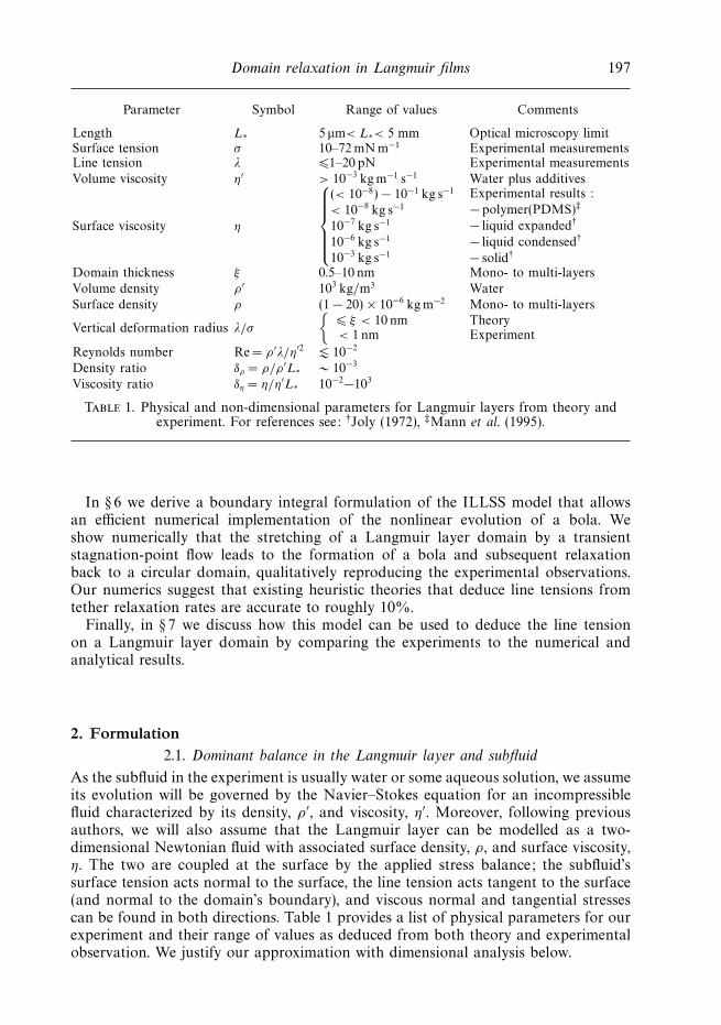
Parameter Symbol Range of values Comments

Length L∗ 5 µm< L∗< 5 mm Optical microscopy limitSurface tension σ 10–72 mN m−1 Experimental measurementsLine tension λ 1–20 pN Experimental measurementsVolume viscosity η′ > 10−3 kgm−1 s−1 Water plus additives

Surface viscosity η

⎧⎪⎪⎪⎪⎨⎪⎪⎪⎪⎩

(< 10−8) − 10−1 kg s−1

< 10−8 kg s−1

10−7 kg s−1

10−6 kg s−1

10−3 kg s−1

Experimental results :

− polymer(PDMS)‡

− liquid expanded†

− liquid condensed†

− solid†

Domain thickness ξ 0.5–10 nm Mono- to multi-layersVolume density ρ ′ 103 kg/m3 WaterSurface density ρ (1 − 20) × 10−6 kgm−2 Mono- to multi-layers

Vertical deformation radius λ/σ

ξ < 10 nm< 1 nm

TheoryExperiment

Reynolds number Re= ρ ′λ/η′2 10−2

Density ratio δρ = ρ/ρ ′L∗ ∼ 10−3

Viscosity ratio δη = η/η′L∗ 10−2−103

Table 1. Physical and non-dimensional parameters for Langmuir layers from theory andexperiment. For references see: †Joly (1972), ‡Mann et al. (1995).

In § 6 we derive a boundary integral formulation of the ILLSS model that allowsan efficient numerical implementation of the nonlinear evolution of a bola. Weshow numerically that the stretching of a Langmuir layer domain by a transientstagnation-point flow leads to the formation of a bola and subsequent relaxationback to a circular domain, qualitatively reproducing the experimental observations.Our numerics suggest that existing heuristic theories that deduce line tensions fromtether relaxation rates are accurate to roughly 10%.

Finally, in § 7 we discuss how this model can be used to deduce the line tensionon a Langmuir layer domain by comparing the experiments to the numerical andanalytical results.

2. Formulation2.1. Dominant balance in the Langmuir layer and subfluid

As the subfluid in the experiment is usually water or some aqueous solution, we assumeits evolution will be governed by the Navier–Stokes equation for an incompressiblefluid characterized by its density, ρ ′, and viscosity, η′. Moreover, following previousauthors, we will also assume that the Langmuir layer can be modelled as a two-dimensional Newtonian fluid with associated surface density, ρ, and surface viscosity,η. The two are coupled at the surface by the applied stress balance; the subfluid’ssurface tension acts normal to the surface, the line tension acts tangent to the surface(and normal to the domain’s boundary), and viscous normal and tangential stressescan be found in both directions. Table 1 provides a list of physical parameters for ourexperiment and their range of values as deduced from both theory and experimentalobservation. We justify our approximation with dimensional analysis below.


2.1.1. Stokesian subfluid

We now propose the ansatz that the relaxation of a polymer domain from, say, abola shape to a circular patch is driven by the line tension, λ, of the patch and thatthe energy is dissipated by the viscosity, η′, of the subfluid. Since the domain Ω isincompressible, say with fixed area A∗, we can choose a linear characteristic domainsize, L∗ ∼

√A∗, and non-dimensionalize the problem based on a characteristic length,

time and mass,

L∗, T∗ =η′(L∗)

2

λ, M∗ = η′L∗T∗ =

(η′)2(L∗)3

λ, (2.1)

respectively.In the bulk of the subfluid, we assume the non-dimensional fluid velocity, u =

uı + vj + wk, is incompressible

∇ · u = 0, (2.2)

and satisfies the non-dimensional Navier–Stokes equations

Re(ut + u · ∇u) = −∇P + ∇2u, (2.3)

where P is the non-dimensional pressure and the Reynolds number

Re =ρ ′λ

(η′)2(2.4)

is assumed to be small; for an aqueous substrate and with a Langmuir-layer linetension λ < 10−11 N we find Re 2 × 10−2.

Consequently, the subfluid velocity satisfies the Stokes equations

∇P = ∇2u (2.5)

at leading order.

2.1.2. Normal stress balance on the surface

We next consider the normal stress balance at the surface. If we allow the surfaceto deform, we need to balance surface tension, pressure and viscous stresses fromthe subfluid, viscous stresses from the Langmuir layer and geometrical contributionsfrom the deforming interface (Aris 1990; Stone & McConnell 1995). However, weargue that at leading order the surface remains flat. To estimate the deformation,we assume that the viscous stresses in the film are smaller than or comparable withthe viscous stresses in the subfluid. Also, the constant atmospheric pressure P0 canbe eliminated by subtracting a constant from the pressure in the fluid. The normalcomponent of the fluid’s stress tensor (which has contributions from the pressure andviscosity) will balance the surface tension. With our non-dimensionalization, we findthat at the surface,

normal viscous stress ∼ surface tension,

η′

T∗∼ σH,

where σ is the surface energy (which may depend upon whether it is inside or outsidethe domain) and H is the mean curvature of the surface. We can solve for themagnitude of the surface curvature,

H ∼ λ

σ (L∗)2. (2.6)


For

L∗ λ/σ (2.7)

we discover that the radius of curvature of the surface is much larger than the typicaldomain size; typically λ/σ ≈ 10 nm so we are looking at domains 10–1000 timeslarger than this length scale. Consequently, we consider the case of a flat surface withthe subfluid occupying the region z < 0 and the Langmuir layer domain Ω containedin the x, y coordinate plane, z = 0, as illustrated in figure 2.

2.1.3. Tangential stress balance in the Langmuir layer domain

For a flat surface, the Langmuir layer evolution equations simplify drastically.Balancing the tangential stresses on the surface yields a force applied by the subfluidon the domain Ω . The non-dimensional stress tensor for our viscous, incompressibleNewtonian fluid is

T = −P I + ∇u + (∇u)T . (2.8)

The tangential stress at the surface acts as a two-dimensional body force, Fs ,(specifically, a force per unit area) acting on the Langmuir layer,

Fs = −k · T · (I − kk) = −[uz ı + vzj ]. (2.9)

As noted above, the normal component of stress at the surface is balanced by surfacetension and produces a negligible deformation of the surface. We assume that theLangmuir layer domain acts like a two-dimensional Newtonian fluid, with this appliedbody force.

2.2. The inviscid Langmuir layer

Using the same non-dimensionalization for the Langmuir-layer surface velocity, U =U ı + V j , and pressure, Π , we see that the velocity field is that of an incompressiblefluid,

∇⊥ · U = 0, (2.10)

where ∇⊥· is the surface divergence. The surface momentum balance yields the two-dimensional Navier–Stokes equation,

δρRe(U t + (U · ∇⊥)U) = Fs + F − ∇⊥Π + δη∇⊥2U, (2.11)

where ∇⊥ is the surface gradient and F is the force associated with the line tension.Following Stone & McConnell (1995) and Lubensky & Goldstein (1996), we modelF as a line force on ∂Ω proportional to the curvature; a specific form is given below.

Assuming a water substrate, we find that

δρ =ρ

ρ ′L∗ 10−3

represents the mass ratio of a portion of the Langmuir layer to the fluid in motionbeneath it; consequently, the inertial forces in the Langmuir layer domain are smallerthan those in the subfluid and are neglected. The ratio

δη =η

η′L∗

represents the ratio of viscous dissipation in the surface to viscous dissipation in thesubfluid; when

L∗ η

η′


we can also neglect the viscous dissipation in the film. The viscosity ratio dependsstrongly on the Langmuir layer and its phases, as can be seen in table 1. The surfaceviscosity has been found experimentally to be negligible for several fluid phases(Mann et al. 1995; Lauger et al. 1996), most explicitly for a polymer (PDMS) wherethe ratio was found to be 10 µm. The parameter can also be adjusted to be assmall as desired by increasing the viscosity of the substrate, which is possible withwater/glycerol mixtures (Mann et al. 1995).

Henceforth we assume that inertial effects and viscous dissipation in the Langmuirlayer are subdominant, so the dominant balance is between the surface pressure, theapplied stress from the subfluid, and the line tension. Balancing the forces with thepressure, we see that

∇⊥Π = Fs + F, (2.12)

which means the Langmuir layer is in hydrostatic equilibrium.To describe the line tension we develop an intrinsic coordinate system on the

surface near the boundary of the domain (see figure 2b). Let Γ (s, t) be a positionvector for the boundary of the domain, ∂Ω , parameterized by the arclength s. Wechoose a right-handed orientation; that is, moving along ∂Ω counterclockwise withΩ to the left corresponds to increasing s. Let t be the corresponding tangent vector.Differentiating with respect to arclength yields d t/ds = κ n, where n is the outward-pointing normal vector and κ is the curvature of ∂Ω (negative for convex Ω). Wedefine the signed distance from ∂Ω along n as d with d < 0 in the interior of Ω andd > 0 in the exterior (Ωc). For sufficiently small |d|, the contours (x, y): d(x, y) = dare curves equidistant from the original ∂Ω , and coordinates for a neighbourhood of∂Ω can be given by the pair (s, d). We can now rewrite the position vector to a pointon the surface in terms of (s, d):

R(s, d) = x(s, d)ı + y(s, d)j = Γ (s, t) + d n. (2.13)

Now, the line tension force can be written as

F = κ nδ(d), (2.14)

where δ(d) is a measure supported on ∂Ω that is a delta function for any curvecrossing ∂Ω transversally. Thus, if we integrate across the boundary, we find that thepressure jump

[Π]d=εd=−ε = κ (2.15)

is proportional to the curvature, as expected.

2.3. The kinematic condition

To complete the formulation we use the kinematic condition to tie the motion ofthe surface to that of the subfluid. As the surface is flat, the vertical velocity at thesurface vanishes,

w(x, y, 0) = 0.

In addition, we assume continuity of the tangential velocity at the surface,

U = U (x, y)ı + V (x, y)j = u(x, y, 0)ı + v(x, y, 0)j . (2.16)

Finally, we also note that the boundary of the domain is advected with the surfacevelocity,

DΓ

Dt= U |∂Ω , (2.17)

where DΓ /Dt is the material derivative of a point on the boundary.


2.4. The inviscid Langmuir-layer Stokesian subfluid approximation (ILLSS)

Under the assumptions that the Langmuir layer is inviscid and the subfluid isStokesian, a complete set of governing equations can be developed. The subfluidvelocity satisfies the Stokes equations

∇ · u = 0, z < 0, (2.18)

∇2u = ∇P, z < 0. (2.19)

In experimental conditions, a Langmuir layer domain, Ω , occupies a small portion ofthe surface area of the subfluid. Thus we assume that the subfluid extends infinitely

far in the horizontal r =√

x2 + y2 and vertical z < 0 directions. If we assume thedomain is finite in extent, the force it applies to the surface is localized and theresponse of the subfluid will decay algebraically in r and exponentially in z (seeStone & McConnell 1995); consequently, we can assume that the velocity u and itsgradients decay uniformly to 0 at ∞:

|u|, |∇u|, |∇2u| → 0 as r2 + z2 → ∞. (2.20)

A second possibility is that the region of interest is embedded in an external flow,such as a transient straining field. We simplify the problem by assuming that theexternal flow, U ext, is irrotational, and uniform in the vertical direction,

U ext = Uext(x, y)ı + Vext(x, y)j , (Vext)x − (Uext)y = 0. (2.21)

In this case, an appropriate boundary condition is that the velocity deviation fromthe imposed flow, u − U ext, and its gradients vanish far from the domain boundary.

The tangential surface stress, Fs , and line tension, F, are in hydrostatic equilibriumwith the surface pressure:

∇⊥Π = Fs + F (2.22)

= −uz(x, y, 0)ı − vz(x, y, 0)j + κ nδ(d). (2.23)

Also, the surface is incompressible:

∇⊥ · U = ux(x, y, 0) + vy(x, y, 0) = 0, (2.24)

which guarantees the area of the domain is conserved. Finally, the kinematic conditionimplies that the normal velocity vanishes at the surface:

w(x, y, 0) = 0, (2.25)

and that the boundary of the domain is advected with the surface velocity:

DΓ

Dt= u|∂Ω . (2.26)

Equations (2.18)–(2.26) completely specify the system.

2.5. Streamfunction formulation for the ILLSS approximation

As noted by both Stone & McConnell (1995) and Lubensky & Goldstein (1996), asignificant simplification can be obtained when motion of the fluid is confined tohorizontal layers; typically this is possible when the Langmuir layer is incompressibleand the viscosities in Ω and Ωc are equal. In the present case, the viscosities are bothzero and the ILLSS model has a solution of this form.


2.5.1. A horizontal flow solution

We begin by introducing a streamfunction ψext(x, y) for the external flow

U ext = k × ∇⊥ψext = −(ψext)y ı + (ψext)x j . (2.27)

Note that as the external flow is irrotational and two-dimensional, the vertical vorticityvanishes:

k · ∇ × U ext = ∇2⊥ψext = 0,

where ∇2⊥ = ∂2

xx + ∂2yy is the horizontal Laplacian.

Next, we look for a solution for the velocity deviation of the subfluid of the form

u − U ext = k × ∇⊥ψ = −ψy ı + ψx j , P = P0, (2.28)

where ψ = ψ(x, y, z) is a streamfunction for the motion in horizontal planes. Inthis case, we discover that the fluid automatically satisfies incompressibility. Taking

the curl of (2.19) shows that the vertical vorticity k · ∇ × u = −∇2⊥ψ is harmonic in

three dimensions and consequently the streamfunction ψ satisfies the ‘twice-harmonic’equation

∇2⊥(∇2ψ) = 0 (2.29)

in the subfluid.From the decay of the velocity deviation in the far field, (2.20), we see that ∇2ψ → 0

as r → ∞. Also, we can deduce from the fact that ∇2⊥(∇2ψ) = 0 (that is that ∇2ψ is

harmonic in each horizontal plane) and Liouville’s Theorem from the analysis of acomplex variable (which states that any harmonic function bounded at infinity mustbe constant) that

∇2ψ = f (z) (2.30)

for some function f (z). A gauge transformation, ψ → ψ + g(z) with gzz = f allowsus to find a solution for ψ that is harmonic in three dimensions,

∇2ψ = 0. (2.31)

The decay of the velocity deviation (2.20) implies that |∇ψ | → 0 as r2 + z2 → ∞.Incompressibility of the fluid (2.18) specifies ∇⊥ · u = 0 in every layer, and at the

surface

0 = −(∇⊥ · u)z = −∇⊥ · uz = ∇⊥ · Fs = ∇2⊥Π − ∇⊥ · F. (2.32)

Consequently, the surface pressure Π is determined by

∇2⊥Π = ∇⊥ · F, (2.33)

where we also specify that |Π | → 0 far from Ω .

2.5.2. Surface-stress streamfunction

We now introduce a streamfunction for the surface stress,

S(x, y) = ψz(x, y, 0),

so the tangential stress balance equation (2.22) becomes (see equation (2.9))

Fs = −uz ı − vzj = −ψyz ı + ψxzj = −k × ∇ψz = −k × ∇S, (2.34)

so that

−k × ∇S = ∇Π − F. (2.35)


Note from (2.33) that Π is harmonic in both Ω and Ωc, and from (2.35) that S andΠ are harmonic conjugates in these regions, so S must be harmonic also. If we takethe vertical component of the curl of (2.35), we find that

∇2S = −∇⊥ · (k × F) (2.36)

= −∇⊥ · (κ tδ(d)) (2.37)

= −κsδ(d), (2.38)

where κs is the derivative of the curvature with respect to arclength.To summarize, in the subfluid, we seek a harmonic streamfunction that satisfies the

surface stress balance

∇2ψ = 0, z < 0, (2.39)

ψz = S, (2.40)

and |∇ψ | → 0 as z → −∞. The surface stress satisfies

∇2⊥S = −κsδ(d) (2.41)

and vanishes in the far field. Finally, the boundary of the domain is advected withthe velocity of the subfluid evaluated at the surface:

DΓ

Dt= U ext + k × ∇⊥ψ

∣∣∣z=0

on ∂Ω, (2.42)

Equations (2.39)–(2.42) specify the evolution of the domain completely. Moreover,computing the boundary velocity has been reduced to solving Laplace’s equation twice,once on the two-dimensional surface and once in the three-dimensional subfluid inthe half-space z < 0.

3. Energy and energy dissipationIn this section we show that in the absence of an external flow (U ext = 0) the ILLSS

model dissipates energy by reducing the arclength of the boundary of the domain.The length of the boundary L is

L(t) =

∮∂Ω

ds.

Then,

Lt = −∮

∂Ω

κ(U · n) ds,

where we have used the fact that the boundary of the domain is advected materiallywith the surface velocity U evaluated on the boundary of the domain ∂Ω . Since thecurvature κ equals the jump in the surface pressure on the domain boundary, we canuse the definition of the delta function to extend the integral to the entire surface.Substituting and using the divergence theorem yields

Lt = −∮

∂Ω

κ(U · n) ds

= −∫ ∫

z=0

U · (κδ(d)n) dx dy

= −∫ ∫

z=0

U · (∇⊥Π − Fs) dx dy. (3.1)


Note that if we integrate the first term over a circle of radius R, then∫ ∫r<R

U · ∇⊥Π dx dy =

∫ ∫r<R

∇⊥ · (ΠU) dx dy

=

∮r=R

Π(U · n) ds

= O(1/R), (3.2)

where the first step employs the incompressibility of the Langmuir layer, and wehave used the fact that the pressure and the velocity are O(1/R) in the far field.Consequently, this term vanishes as R → ∞.

Rewriting the remaining term in terms of the surface stress, we find

Lt =

∫ ∫z=0

u · Fs dx dy = −∫ ∫

z=0

uuz + vvz dx dy.

We now use a standard identity for Stokes flow by extending the surface to a largeclosed hemisphere and noting that the velocity vanishes far from the domain. Thedivergence theorem yields the standard result (cf. Aris 1990; Lubensky & Goldstein1996) that

Lt = −1

2

∫ ∫ ∫z<0

|eij |2 dx dy dz, (3.3)

where eij is the rate-of-strain tensor

eij =1

2

(∂ui

∂xj

+∂ui

∂xj

), (3.4)

by which we see that the arclength of the boundary decreases monotonically, unlessthe fluid is at rest. The action of the flow is to minimize the length of the boundarywhile preserving the area of the domain; the isoperimetric inequality suggests that,for domains of finite area, Ω will relax to a circle, or possibly the union of multiplecircular domains. If we allow the domain to be infinite, a half-plane or an infinitestrip could also be a (possibly local) energy minimizer.

4. Stability and relaxation to a circular domainIn this section we consider the relaxation of a linear perturbation to the boundary

of a circular domain Ω of radius R. We know from the previous section that a circulardomain is stable. However, rates of relaxation of the various modes are characteristicand give one possible way of measuring line tension (Mann et al. 1995). We expandthe perturbation in Fourier modes, substitute in the governing equations, and retaineach mode to first order in the perturbation.

We describe the boundary of the domain in polar coordinates as

R(θ, t) = R + εβ(θ, t). (4.1)

Rotational symmetry guarantees that angular Fourier modes will decouple in thelinear stability problem. Moreover, area conservation of the domain requires that then = 0 mode vanishes. Consequently, we expand β in the form

β(θ, t) =

∞∑n=1

[an cos(nθ) + bn sin(nθ)] eλnt (4.2)

and compute to first order in ε.


Linearizing the curvature operator using standard identities, we find

κ(R) = − 1

R+ ε

1

R2(βθθ + β) + O(ε2), (4.3)

κs(R) =ε

R3(βθθθ + βθ ) + O(ε2), (4.4)

and thus

κs(R) = ε

∞∑n=1

[−an sin(nθ) + bn(t) cos(nθ)]n(1 − n2)

R3eλnt (4.5)

to first order in ε. We can now solve for the linearized surface-stress streamfunction;let

S(r, θ, t) = ε∑n=1

[an sin(nθ) − bn cos(nθ)]n(1 − n2)

R3eλnt sn(r). (4.6)

Substituting into Laplace’s equation (2.41) for the surface stress yields

Lr sn(r) ≡(

∂2

∂r2+

1

r

∂

∂r− n2

)sn(r) = δ(r − R), (4.7)

where sn must be regular at the origin and vanish in the far field. Note that at leadingorder the δ-function forcing can be applied at the unperturbed boundary (R = R).Solving for sn(r), we find

sn(r) =

−R/2n(r/R)n, r < R,

−R/2n(R/r)n, r > R.(4.8)

To solve for the subfluid streamfunction, let

ψ(r, θ, z, t) = −ε

∞∑n=1

[an sin(nθ) − bn cos(nθ)]eλnt(1 − n2)

2R2Pn(r, z), (4.9)

where Pn(r, z) satisfies Laplace’s equation (2.39) in the subfluid:(Lr +

∂2

∂z2

)Pn(r, z) = 0, z < 0, (4.10)

∂Pn

∂z(r, 0) = fn(r) ≡

(r/R)n, r < R,

(R/r)n, r > R,(4.11)

and Pn → 0 for r → ∞ and z → −∞. Once again as we are only retaining linearperturbations we may evaluate the surface-stress boundary condition for the circulardomain, ignoring the deformation of the boundary.

As solutions to Laplace’s equation in the subfluid take the form Jn(kr)ekz, we canconstruct the solution to the problem via a Hankel transform,

Pn(r, z) =

∫ ∞

0

cn(k)Jn(kr)ekz dk, (4.12)

which implies

∂Pn

∂z(r, 0) =

∫ ∞

0

cn(k)Jn(kr) k dk = fn(r). (4.13)


Inverting the transform with the identity

δ(k − k′) =

∫ ∞

0

krJn(kr)Jn(k′r) dr (4.14)

yields

cn(k) =

∫ ∞

0

fn(r)Jn(kr) r dr, (4.15)

or

Pn(r, z) =

∫ ∞

0

∫ ∞

0

fn(r′)Jn(kr ′)Jn(kr)ekz r ′ dr ′ dk. (4.16)

To complete the problem, we use the kinematic condition to advect the domainboundary. We linearize around R = R,

Rt = εβt = − 1

Rψθ (R, θ). (4.17)

Substituting the expressions (4.2) and (4.9) for β and ψ yields

∞∑n=1

[an cos(nθ) + bn sin(nθ)]λneλnt

=

∞∑n=1

[an cos(nθ) + bn sin(nθ)]eλntn(1 − n2)

2R3Pn(R, 0),

from which we deduce

λn =n(1 − n2)

2R3Pn(R, 0). (4.18)

However,

Pn(R, 0) =

∫ ∞

0

∫ ∞

0

fn(r′)Jn(kr ′)Jn(kR) r ′ dr ′ dk

= R

∫ ∞

0

[∫ 1

0

(ρ)n+1Jn(kρ) +

∫ ∞

1

(ρ)−n+1Jn(kρ) dρ

]Jn(k) dk

= 2nR

∫ ∞

0

[Jn(k)]2dk

k2

=2nR

π(n2 − 14),

which allows a closed form for the relaxation rates,

λn = − n2(n2 − 1)

πR2(n2 − 1

4

) , for n = 1, 2, 3 . . . . (4.19)

This result can also be deduced from Stone & McConnell (1995) as reported in Mannet al. (1995) where it was used to estimate the line tension from the relaxation rate ofperturbations to a circular domain. Note that λ1 = 0 corresponds to the translationsymmetry of the domain, and λn < 0 for n 2, as expected, confirming that thecircular domain is stable.


5. Linear stability of a tetherThe length of a tether between the two bola of a deformed domain Ω (see

figure 1) can be orders of magnitude longer than wide. It can thus be reasonablyapproximated by a two-dimensional infinite strip in the surface of the subfluid. In thissection we consider the relaxation of linear perturbations of an infinite strip of width2d . Consider a domain occupying the region −d y d . We consider two classesof linear perturbations: varicose perturbations for which the domain is symmetricaround the line y = 0 and sinuous instabilities for which the perturbations areantisymmetric. The analysis is analogous to that of the previous section – expandingthe perturbations in Fourier modes and solving to first order in the perturbation.The growth rates for the sinuous perturbation can be deduced from the results ofDeKoker & McConnell (1996) who analysed stripe patterns in an analogous lipidsystem.

For the varicose case, we assume the domain takes the form

|y| < H (x, t) = d + εh(x, t). (5.1)

Translational symmetry guarantees that Fourier modes in x decouple. Consequently,we expand h(x, t) in the form

h(x, t) =

∫ ∞

−∞h(k)eikx+λk t dk. (5.2)

We linearize the curvature operator; using standard identities, we find that on theupper boundary

κ = εhxx + O(ε2), (5.3)

κs = −εhxxx + O(ε2), (5.4)

from which we derive

κs = ε

∫ ∞

−∞ik3 h(k)eikx+λk t dk, (5.5)

where we have dropped terms of order ε2 and higher. To solve for the linearizedsurface-stress streamfunction, let

S(x, y, t) = ε

∫ ∞

−∞ik3 S(k, y)eikx+λk t dk. (5.6)

Laplace’s equation (2.41) for the surface stress implies(∂2

∂y2− k2

)S(k, y) = −[δ(y − d) − δ(y + d)] (5.7)

with |S(k, y)| → 0 as |y| → ∞. Solving,

S(k, y) =

⎧⎪⎨⎪⎩

(e−|k|y/k

)sinh(kh), d y,(

e−|k|d/k)sinh(ky), |y| < d,

−(e|k|y/k

)sinh(kh), y −d.

(5.8)

We now solve for the subfluid streamfunction; let

ψ(x, y, z, t) = ε

∫ ∞

−∞ik2 P (k, y, z)eikx+λk t dk, (5.9)


where P (k, y, z) must satisfy Laplace’s equation (2.39) in the subfluid:(∂2

∂y2+

∂2

∂z2− k2

)P (k, y, z) = 0, z < 0, (5.10)

∂P

∂z(k, y, 0) = f (k, y) ≡

⎧⎪⎨⎪⎩

e−|k|y sinh(kh), d y,

e−|k|d sinh(ky), |y| < d,

−e|k|y sinh(kh), y −d.

(5.11)

and P (k, y, z) vanishes as z → −∞. Note that as we are only retaining linearperturbations we may evaluate the surface-stress boundary condition at z = ±d ,ignoring the perturbations to the boundary.

Solutions to Laplace’s equation in the subfluid take the form exp(iy +√

k2 + 2z),so we construct the general solution to the problem:

P (k, y, z) =

∫ ∞

−∞c(k, ) eiy+

√k2+2z d. (5.12)

Thus

∂P

∂z(k, y, 0) =

∫ ∞

−∞

√k2 + 2 c(k, )eiy d = f (k, y). (5.13)

Inverting the Fourier transform yields

c(k, ) =1

2π√

k2 + 2

∫ ∞

−∞f (k, y)e−iy dy. (5.14)

To complete the problem, we use the kinematic condition to advect the domainboundary. Linearizing around z = d we find

Ht = εht = −ψx(x, d, 0). (5.15)

Substituting the expressions (5.2) and (5.9) for h and ψ , we find∫ ∞

∞λkh(k)eikx+λk t dk = −

∫ ∞

−∞k3 P (k, d, 0)eikx+λk t dk, (5.16)


λk = −k3P (k, d, 0). (5.17)

However

P (k, d, 0) =1

2π

∫ ∞

−∞

eid

√k2 + 2

∫ ∞

−∞f (k, y ′)e−iy ′

dy ′ d

=

∫ ∞

−∞f (k, y ′)

[1

2π

∫ ∞

−∞

e−i(y ′−d)

√k2 + 2

d

]dy ′

=1

π

∫ ∞

−∞f (k, y ′)K0(|k(d − y ′)|) dy ′,


λk = −k2

πIv(|kd|), (5.18)

where

Iv(α) = α

∫ ∞

−∞F (α, ξ )K0(α|1 − ξ |) dξ (5.19)


and

F (α, ξ ) ≡

⎧⎨⎩

e−αξ sinh(α), 1 ξ,

e−α sinh(αξ ), |ξ | < 1,

−eαξ sinh(α), ξ −1.

(5.20)

A laborious calculation reduces this to

Iv(α) = 1 − cosh(2α) +

∫ 2α

0

sinh(2α − ζ )K0(ζ ) dζ = 1 − 2αK1(2α). (5.21)

Note for α 1, we find

Iv(α) = α2(1 − 2γ − 2 ln(α)) + α4(

54

− γ − ln(α))

+ O(α6 lnα),

where γ denotes Euler’s constant. Also, as is clear from figure 3, |Iv(α)| < 1 and asα → ∞, we see that Iv(α) increases monotonically to 1.

For the sinuous case, we will assume the perturbations to the domain areantisymmetric at leading order,

−d + εh(x, t) < y < d + εh(x, t). (5.22)

We again expand h(x, t) in the form

h(x, t) =

∫ ∞

−∞h(k)eikx+λk t dk. (5.23)

A similar calculation yields

λk = −k2

πIs(|kd|), (5.24)

Is(α) = α

∫ ∞

−∞G(α, ξ )K0(α|1 − ξ |) dξ, (5.25)

and

G(α, ξ ) ≡

⎧⎨⎩

e−αξ cosh(α), 1 ξ,

e−α cosh(αξ ), |ξ | < 1,

eαξ cosh(α), ξ −1.

(5.26)

We find after some calculation that

Is(α) = 2 − Iv(α) = 1 + 2αK1(2α).

Consequently, for α 1, we find

Is(α) = 2 + α2(2γ − 1 + 2 ln(α)) + α4(γ − 5

4+ ln(α)

)+ O(α6 lnα),

where γ again denotes Euler’s constant. As α increases from 0, Is(α) decreasesmonotonically from 2 to 1.

In the paper by DeKoker & McConnell (1996), the drag a sinuous perturbationfeels due to the subfluid is computed, and a simple calculation yields the decay ratecomputed above. Moreover, by interpreting these results as a balance between thedrag and the line tension forcing, and noting that the subfluid drag is linear, we candeduce that averaging a sinuous and varicose perturbation is equivalent to perturbingthe edge of a half-plane sinusoidally. This yields the result

12[Is(α) + Iv(α)] = 1,

where the 1 on the right-hand side arises from the half-plane problem which isequivalent to the limit of large α in both the sinuous and varicose problems.


2.0

1.5

1.0

0.5

0 0.5 1.0 1.5 2.0 2.5 3.0α

Is(α)

Iv(α)

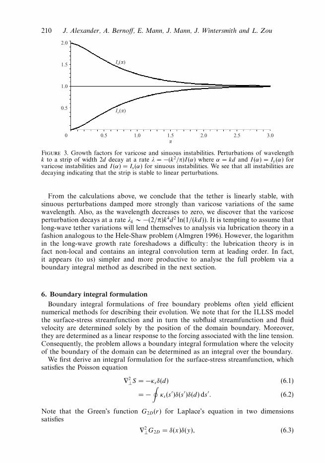
Figure 3. Growth factors for varicose and sinuous instabilities. Perturbations of wavelengthk to a strip of width 2d decay at a rate λ = −(k2/π)I (α) where α = kd and I (α) = Iv(α) forvaricose instabilities and I (α) = Is(α) for sinuous instabilities. We see that all instabilities aredecaying indicating that the strip is stable to linear perturbations.

From the calculations above, we conclude that the tether is linearly stable, withsinuous perturbations damped more strongly than varicose variations of the samewavelength. Also, as the wavelength decreases to zero, we discover that the varicoseperturbation decays at a rate λk ∼ −(2/π)k4d2 ln(1/(kd)). It is tempting to assume thatlong-wave tether variations will lend themselves to analysis via lubrication theory in afashion analogous to the Hele-Shaw problem (Almgren 1996). However, the logarithmin the long-wave growth rate foreshadows a difficulty: the lubrication theory is infact non-local and contains an integral convolution term at leading order. In fact,it appears (to us) simpler and more productive to analyse the full problem via aboundary integral method as described in the next section.

6. Boundary integral formulationBoundary integral formulations of free boundary problems often yield efficient

numerical methods for describing their evolution. We note that for the ILLSS modelthe surface-stress streamfunction and in turn the subfluid streamfunction and fluidvelocity are determined solely by the position of the domain boundary. Moreover,they are determined as a linear response to the forcing associated with the line tension.Consequently, the problem allows a boundary integral formulation where the velocityof the boundary of the domain can be determined as an integral over the boundary.

We first derive an integral formulation for the surface-stress streamfunction, whichsatisfies the Poisson equation

∇2⊥S = −κsδ(d) (6.1)

= −∮

κs(s′)δ(s ′)δ(d) ds ′. (6.2)

Note that the Green’s function G2D(r) for Laplace’s equation in two dimensionssatisfies

∇2⊥G2D = δ(x)δ(y), (6.3)


which yields

G2D(r) =1

2πln r, r =

√x2 + y2.

As (s, d) are orthogonal coordinates at the boundary of the domain, we can constructa solution for the surface-stress streamfunction in terms of the Green’s function,

S(x, y) = −∮

κs(s′)G2D(|R − Γ (s ′)|) ds ′, R = x ı + yj , (6.4)

= − 1

4π

∮κs(s

′) ln |R − Γ (s ′)|2 ds ′ (6.5)

= − 1

2π

∮κ(s ′)

[Γ s(s′)] · [R − Γ (s ′)]

|R − Γ (s ′)|2 ds ′, (6.6)

where the last step is derived via integration by parts.This can be simplified by introducing a vector, q, in the surface from a point on

the boundary of the domain (Γ ) to an arbitrary point the surface (R),

q(s) = R − Γ (s), q = |q|, q =qq

, (6.7)

which allows us to write the solution for the surface-stress streamfunction as

S(x, y) = − 1

2π

∮κ t · q

qds, (6.8)

where we have used the fact that Γ s is the unit tangent t .The subfluid streamfunction ψ(x, y, z) can now be solved for in terms of S(x, y);

we know the solution is harmonic with a Neumann condition at the surface,

∇2ψ = 0, z < 0, (6.9)

ψz = S(x, y), z = 0, (6.10)

and the fluid speed |∇ψ | vanishes as z → −∞.The associated Green’s function G3D(x, y, z), which satisfies

∇2G3D = 0, z < 0, (6.11)

∂z(G3D) = δ(x)δ(y), z = 0, (6.12)

is easily derived, namely,

G3D(x, y, z) =1

2π

1√z2 + r2

, r =√

x2 + y2,

which in turn implies

ψ(x, y, z) =

∫ ∞

−∞

∫ ∞

−∞S(x ′, y ′)G3D(x − x ′, y − y ′, z) dx ′ dy ′. (6.13)

It is now straightforward, if algebraically cumbersome, to substitute the expressionfor the surface-stress streamfunction into this integral formulation (evaluated at thesurface), and exchange the order of integration to derive the streamfunction evaluated


at the surface. We see that

ψ(x, y, 0) =

∫ ∞

−∞

∫ ∞

−∞S(x ′, y ′)G3D(x − x ′, y − y ′, 0) dx ′ dy ′

= − 1

2π

∫ ∞

−∞

∫ ∞

−∞

[∮κt · q

qds

]G3D(x − x ′, y − y ′, 0) dx ′ dy ′

=

∮κt · K (Γ (s), R) ds,

where

K (R′, R′′) = − 1

(2π)2

∫ ∞

−∞

∫ ∞

−∞

R′ − R|R′ − R|2|R′′ − R| dx dy (6.14)

=1

2π

R′ − R′′

|R′ − R′′| . (6.15)

The last integral above can be evaluated by changing to polar coordinates with originat R′ and with R′′ along the polar axis, evaluating the radial integral on a finitedisk centred at the origin, evaluating the angular integral and then letting the radiusapproach infinity. Consequently, we conclude that

ψ(x, y) = − 1

2π

∮κ t · q ds, q =

R − Γ (s)

|R − Γ (s)| , R = x ı + yj . (6.16)

To finish the formulation we must specify the motion of the boundary; from thekinematic condition (2.42) we know

DΓ

Dt= (U + U ext)|∂Ω = (k × ∇⊥ψ + U ext)|∂Ω. (6.17)

At this point we turn our attention from the physical calculation to setting up thenumerical calculation of the boundary integral formulation. We first parameterize theboundary, Γ (p, t), with a parameter p which is 2π-periodic. We then note that asthe boundary is isotropic, we are free to introduce an arbitrary tangential velocitywhose only effect will be to change the parameterization of the boundary (cf. Houet al. 1994). Consequently, the tangential component, V, can be chosen arbitrarily(and in fact will be used to distribute the collocation points evenly on the boundary).So an equivalent formulation is

Γ t = (U + Uext)n + V t, (6.18)

where

Uext = n · U ext, (6.19)

U = n · k × ∇⊥ψ |∂Ω = ψs |∂Ω, (6.20)

and V is arbitrary. It now suffices to know the streamfunction only on the boundaryof the domain; this simplifies our numerical calculations immensely.

In summary, we find that

Γ t = (Ψs + Uext)n + V t, (6.21)

where Ψ (s) is the streamfunction restricted to the boundary of the domain,

Ψ (s) = − 1

2π

∮κ t · Q ds ′, Q =

Γ (s ′) − Γ (s)

|Γ (s ′) − Γ (s)| , (6.22)


and V can be chosen arbitrarily. Once the externally imposed velocity U ext and theinitial domain boundary location have been specified, the boundary integral equations(6.21), (6.22) completely determine the evolution of the Langmuir layer.

6.1. Boundary integral numerics

We report on a continuing effort to numerically simulate the boundary integralequations (6.21), (6.22). Our method is based on the work of Hou et al. (1994)who recognized the importance of using an intrinsic description of the boundarywhich allows an accurate implicit solution for the high-wavenumber modes avoidingnumerical instabilities. Figures 4, 5 illustrate that such a method reproduces theobserved bola dynamics qualitatively; we expect to report a quantitative comparisonelsewhere after we have refined our numerical simulations and experimental technique.

Previously a boundary integral formulation for the Langmuir layer (includingelectrostatic forces) was proposed by Lubensky & Goldstein (1996) and implementedby Heinig et al. (2004); they compute the boundary velocity explicitly, which is

equivalent to computing k × ∇⊥ψ in (6.16), (6.17). Heinig et al. (2004) were ableto qualitatively reproduce many experimental results, although the scheme exhibitedmoderate area loss. Moreover, their scheme was explicit and first-order in time whichlimits the size of time-steps that can be taken accurately. Here we present a schemethat is second-order in time, essentially spectrally accurate in space, and semi-implicitwhich guarantees stability. Moreover, by using the conservative form of the boundaryintegral equations (6.21), (6.22) where the velocity is an exact derivative with respectto arclength our scheme better conserves the area of the domain.

Following Hou et al. (1994), we represent the boundary with an equal-arclengthdiscretization; note that this equal-arclength constraint specifies the tangentialvelocity. Derivatives are computed pseudo-spectrally (Gottlieb & Orszag 1977;Trefethen 2000), and the boundary integral is computed using either Rombergintegration or a 16-panel closed Newton–Cotes formula which guarantees high-orderspatial accuracy. Numerically we see that the problem is extremely stiff and explicitintegration methods are highly susceptible to high-wavenumber instabilities. This canbe ameliorated by operator splitting following the ideas of Hou et al. (1994). Whilesuch a splitting is not immediately apparent in the formulation above, the formulationin Lubensky & Goldstein (1996) and Heinig et al. (2004) can be used to show thatasymptotically the high wavenumbers are governed by a much simpler evolution law,namely motion by mean curvature. It is straightforward to solve the evolution bymean curvature implicitly and to high accuracy (cf. Hou et al. 1994). We proceedby using Strang splitting with the mean-curvature step implemented implicitly andthe external velocity and the boundary integral velocity minus the mean curvaturevelocity computed explicitly.

We implemented this algorithm using MATLAB. Numerically, we found that it wasnecessary to correct the arclength discretization regularly to correct a slow drift ofthe grid points – this was done using spectral interpolation and a Newton–Raphsoniteration. Also, it is necessary to filter the highest wavenumber modes in the boundaryintegral (whose numerical accuracy is poor anyway due to the discretization); inpractice we convolute the spectrum with a smooth filter and retain roughly two-thirdsof the spectrum. Details of the numerical implementation can be found in Pugh(2006).

The specific numerical integration illustrated in figures 4, 5 uses 1024 points and 64time-steps per unit of time. The domain initially is a circle of radius 3. An externalstraining flow U ext = 0.25(x ı − yj ) is imposed and the domain is stretched into a


t = 0

Tim

e

(End of stretching)

Figure 4. A series of snapshots of a numerical evolution of the stretching of a Langmuirdomain computed via a boundary integral method for the inviscid Langmuir layer Stokesiansubfluid Model. The domain is originally a circle of radius 3. At the end of the stretching thedomain is 60 units long. The domain is stretched by a transient straining flow of strength 0.25for 11.14 units of time; snapshots are separated by 1.59 units of time.

long narrow lozenge of length 60 with an aspect ratio of roughly 144-to-1. As thedomain relaxes it loses convexity with the appearance of two rounded reservoirs atthe tips connected by a narrow tether, creating the classic bola shape observed in theexperiments. Eventually the domain regains convexity, becomes nearly elliptical, andrelaxes towards the circular energy minimizer.

This numerical run took about thirty hours on a GHz speed single-processormachine. A check on the accuracy of the code is that the area of the domain shouldbe conserved; during the stretching phase the domain loses roughly 1% of its area;during the relaxation phase the area is conserved to within 0.1%.

6.2. Computing the line tension

In this section we show how to compute the line tension from the tether relaxationvelocity. Experiments on bola relaxation have been used previously to make order-of-magnitude estimates of line tensions (Benvegnu & McConnell 1992; Mann et al.1992, 1995). Benvegnu & McConnell (1992) modelled the bola as a circular disk beingpulled by the line tension associated with the tether. By computing the force exertedby the line tension and balancing it with the drag on the disk they estimate the linetension. We summarize their calculation below; note that we have returned to theoriginal dimensional variables.


(End of streching)

Tim

e

Figure 5. Tether relaxation. After the straining field is released in figure 4, the domainassumes the classic bola shape, and eventually relaxes back to an ellipse approaching theenergy-minimizing circular configuration. Here the snapshots are separated by 13.1 units oftime. A movie of this numerical evolution is available with the online version of the paper.

The total horizontal force on the disk, Fline, is easily computed by integrating theforce around one end of the tether. For definiteness, consider the right half of one thetethers in figure 5 and integrate along a contour C from the midpoint of the bottomof the tether counter-clockwise to the midpoint of the top of the tether,

Fline =

∫Cλκ n ds = λ t

∣∣top

bottom= −2λj , (6.23)

yielding a force proportional to the line tension in the direction of motion.The drag force is the product of the bola velocity and the drag coefficient,

Fdrag = CdragVbolaj .


1.50

1.25

1.00

0.75

0.50

Ebola

0 50 100 150Time, t

Figure 6. Computing line tension from the tether relaxation. Previous studies have assumedthat the line tension for a relaxing tether can be computed from λ = Ebola4η′VbolaRbola whereVbola is the bola velocity and Rbola is the tether radius, measured as the maximum half-widthof the bola perpendicular to the tether. Here we plot Ebola for the numerically computedrelaxation in figure 5; the graph starts when the straining flow stops at t = 11.14 and stopswhen the domain loses convexity at roughly t = 144.5. Previous studies assumed that Ebola

was unity after the initial relaxation and before the two bolas merge. In fact it slowly increasesfrom approximately 1 to a maximum of 1.3 in the regime where the ends of the bola areinteracting. These results suggest that Mann et al. (1995) underestimates the line tension byperhaps 20%.

The drag coefficient was approximated by Benvegnu & McConnell (1992) in twoways: first as half the drag on a flat disk of radius Rbola in an infinite fluid, whichyields Cdrag = 16

3η′Rbola (cf. section 339, Lamb 1932); the second model considers the

drag on a solid disk in an inviscid monolayer on an infinite subfluid, which yieldsCdrag = 8η′Rbola (cf. Hughes et al. 1981).

We can now solve for the line tension by equating Fline and Fdrag; this yields

λ = Ebola4η′VbolaRbola, (6.24)

where Ebola = Cdrag/8, which is 2/3 for the first model and unity for the secondmodel. Typically Rbola is estimated as half the maximum width of the bola measuredperpendicular to the tether axis.

Figure 6 allows us to estimate Ebola from our numerical simulations; as we havenon-dimensionalized the problem we can set the viscosity and line tension to unity toyield

Ebola =1

4VbolaRbola

.

We assume that this model should be valid at times after the domain has relaxed toa bola shape and before the two ends of the bola have begun to interact. In fact wefind that Ebola rapidly increases to slightly above unity as the ends of the bola becomebulbous. It then slowly increases to a maximum of roughly 1.3 where the two endsof the tether are clearly interacting. This suggests that choosing Cdrag = 8η′Rbola isnearly correct and that the results of Mann et al. (1995) which use this approximationunderestimate the line tension by perhaps 20%. Our simulations also suggest thatvariations in bola length and tether thickness can cause changes in the relaxation rateof the same order; this effect is explored in Pugh (2006).


7. DiscussionIn this paper we have developed a model of a Langmuir layer with two fluid

phases, one of which is localized into a compact domain. Dimensional analysissuggests that the dominant balance is between the driving line tension at thedomain boundary and the viscous drag of the subfluid. The governing hydrodynamicequations have been reduced to a more tractable form: the inviscid Langmuir layerStokesian subfluid (ILLSS) model discussed herein reduces the problem to solving fora horizontal streamfunction which is harmonic in the subfluid, and the surface-stressstreamfunction which is harmonic in the Langmuir layer domains. A further reductionyields a boundary integral formulation which can be efficiently numerically integrated.The model conforms well to experimentally observed behaviour of Langmuir layers.

The dissipation of energy suggests that an isolated compact domain will evolvetowards a circular equilibrium which minimizes its perimeter. It is also possible tocompute the relaxation rates of perturbations of a circular domain, which has beenan effective tool for estimating line tensions (Mann et al. 1992, 1995; Lauger et al.1996). In particular the amplitude of the nth Fourier mode decays as exp(−t/τn)where τn is the characteristic relaxation time,

τn =πR2η′

λ

(n2 − 1

4

)n2(n2 − 1)

, for n = 1, 2, 3 . . . , (7.1)

where πR2 is the domain area, η′ is the subfluid viscosity and λ is the line tension.These relaxation rates are deduced from (4.19) and agree with equation (A18) inMann et al. (1995) which was based on the earlier work of Stone & McConnell(1995).

We also consider perturbations of an infinite strip as a model of the narrowtether seen in the bola configuration. Linear theory indicates that the infinite stripis stable to perturbations, in agreement with the experimental observation of tethers.A logical next analytical step is to pursue a nonlinear lubrication theory model oflong-wave perturbations to the tether; this is a strategy that works well, for example,for analysing rupture in the Hele-Shaw problem (Almgren 1996; Almgren et al. 1996;Constantin et al. 1993; Dupont et al. 1993; Goldstein et al. 1993). However, ouranalysis (not reported here) shows that the lubrication model for this problem isnon-local and contains an integral term which makes the analysis quite complicated.A simpler alternative is to convert the problem to a boundary integral formulationand attack it numerically.

In the penultimate section of this paper we derive a boundary integral formulationfor the ILLSS model which is capable of incorporating an external irrotational flow.Our numerical implementation of a circular patch in a stagnation-point flow showsthat it is stretched into a long and narrow filament. When the stagnation flow is turnedoff, the domain first develops circular bulges at its ends, creating the characteristicbola shape. The bulbous ends then slowly migrate towards each other, eventuallymerging and relaxing to a circular domain, the ubiquitous energy minimizer.

Experiments on bola relaxation have been used previously to make order-of-magnitude estimates of line tensions (Benvegnu & McConnell 1992; Mann et al.1992, 1995). However these estimates rely on heuristic theories and dimensionalanalysis; our numerical simulation suggest that Mann et al. (1995) underestimate linetensions by perhaps 20% which is similar to the reported experimental uncertainty.

We believe comparisons of the fully nonlinear numerical simulation to theexperimental observations of bola relaxation will allow a more accurate determination


of the line tension in a variety of systems. Unlike relaxation rates for perturbationof a circular domain, these measurements are not limited to the regime where lineartheory is applicable. In conclusion, we believe that the ILLSS model effectively modelsmany experimental observations of Langmuir layers while remaining analytically andnumerically tractable.

The authors would like to thank the referees for their careful and cogent commentson an earlier draft of this paper. A. J. B. and J.R.W. would like to thank HarveyMudd College for financial support and UCLA for summer support via NSF grantsDMS-0535521 and ACI-0321917, and ONR grant N000140410078. L. Z. and E.K.M.were partially supported by the National Science Foundation under Grant No. DMR-9984304.

REFERENCES

Adamson, A. W. & Gast, A. P. 1998 Physical Chemistry of Surfaces, 6th Edn. John Wiley and Sons.

Almgren, R. 1996 Singularity formation in Hele-Shaw bubbles. Phys. Fluids 8, 344–352.

Almgren, R., Bertozzi, A. & Brenner, M. P. 1996 Stable and unstable singularities in the unforcedHele-Shaw cell. Phys. Fluids 8, 1356–1370.

Aris, R. 1990 Vectors, Tensors, and the Basic Equations of Fluid Mechanics . Dover.

Benvegnu, D. J. & McConnell, H. M. 1992 Line tension between liquid domains in lipidmonolayers. J. Phys. Chem. 96, 6820–6824.

Brochard-Wyart, F. 1990 Stability of a liquid ribbon spread on a liquid surface. C. R. Acad. SciIi 311, 295–300.

Constantin, P., Dupont, T. F., Goldstein, R. E., Kadanoff, L. P., Shelley, M. J. & Zhou, S.-M.

1993 Droplet breakup in a model of the Hele-Shaw cell. Phys. Rev. E 47, 4169–4181.

DeKoker, R. & McConnell, H. M. 1993 Circle to dogbone—shapes and shape transitions of lipidmonolayer domains. J. Phys. Chem. 97, 13419–13424.

DeKoker, R. & McConnell, H. M. 1996 Stripe phase hydrodynamics in lipid monolayers. J. Phys.Chem. 100, 7722–7728.

Drazin, P. G. & Reid, W. H. 2004 Hydrodynamic Stability, 2nd Edn. Cambridge University Press.

Dupont, T. F., Goldstein, R. E., Kadanoff, L. P. & Zhou, S.-M. 1993 Finite-time singularityformation in Hele-Shaw systems. Phys. Rev. E 47, 4182–4196.

Edidin, M. 2003 The state of lipid rafts: From model membranes to cells. Annu. Rev. Biophys.Biomol. Structure 32, 257–283.

Gaines Jr, G. L. 1966 Insoluble Monolayers at Liquid-Gas Interfaces . Interscience.

Glasner, K. 2003 A diffuse interface approach to Hele-Shaw flow. Nonlinearity 16, 49–66.

Goldstein, R. E., Pesci, A. I. & Shelley, M. J. 1993 Topology transitions and singularities inviscous flows. Phys. Rev. Lett. 70, 3043–3046.

Goodrich, F. C. 1981 The theory of capillary excess viscosities. Proc. R. Soc. Lond. A 374, 341–370.

Gottlieb, D. & Orszag, S. A. 1977 Numerical Analysis of Spectral Methods: Theory and Applications .Society for Industrial and Applied Mathematics.

Heinig, P., Helseth, L. E. & Fischer, T. M. 2004 Relaxation of patterns in 2D modulated phases.New J. Phys. 6, 189.

Hou, T., Lowengrub, J. & Shelley, M. 1994 Removing the stiffness from interfacial flow withsurface tension. J. Comput. Phys. 114, 312–338.

Hughes, B. D., Pailthorpe, B. A. & White, L. R. 1981 The translational and rotational drag on acylinder moving in a membrane. J. Fluid Mech. 110, 349–372.

Joly, M. 1972 Rheological properties of monomolecular films: Part ii: Experimental results.theoretical interpretation. applications. Surface Colloid Sci. 5, 79–193.

Lamb, H. 1932 Hydrodynamics . Cambridge University Press.

Lauger, J., Robertson, C. R., Frank, C. W. & Fuller, G. G. 1996 Deformation and relaxationprocesses of mono- and bilayer domains of liquid crystalline langmuir films on water. Langmuir12 (23), 5630–5635.


Lubensky, D. K. & Goldstein, R. E. 1996 Hydrodynamics of monolayer domains at the air-waterinterface. Phys. Fluids 8, 843–854.

Lucassen, J., Akamatsu, S. & Rondelez, F. 1991 Formation, evolution, and rheology of 2-dimensional foams in spread monolayers at the air-water interface. J. Colloid Interface Sc.144, 434–448.

Mann, E. K. 1992 PDMS films at water surfaces: texture and dynamics. PhD thesis, Universite deParis VI.

Mann, E. K., Henon, S. & Langevin, D. 1992 Meunier molecular layers of a polymer at the freewater surface: Microscopy at the Brewster angle. J. Phys. Paris 2, 1683–1704.

Mann, E. K., Henon, S., Langevin, D., Meunier, J. & Leger, L. 1995 The hydrodynamics ofdomain relaxation in a polymer monolayer. Phys. Rev. E 51, 5708–5720.

Mann, E. K. & Primak, S. 1999 The stability of two-dimensional foams in Langmuir monolayers.Phys. Rev. Lett. 83, 5397–5400.

Mann Jr, J. A. 1985 Dynamics, structure and function of interfacial regions. Langmuir 1, 10–23.

Mann Jr, J. A., Crouser, P. D. & Meyer, W. V. 2001 Surface fluctuation spectroscopy by surface-light-scattering spectroscopy. Appl. Optics 40 (24), 4092–4112.

Mayor, S. & Rao, M. 2004 Rafts: Scale-dependent, active lipid organization at the cell surface.Traffic 5, 231–240.

de Mul, M. N. G. & Mann Jr, J. A. 1998 Determination of the thickness and optical properties ofa langmuir film from the domain morphology by Brewster angle microscopy. Langmuir 14,2455–2466.

Parton, R. G. & Hancock, J. F. 2004 Lipid rafts and plasma membrane microorganization: Insightsfrom Ras. Trends Cell Biol. 14 (3), 141–147.

Powers, T. R., Huber, G. & Goldstein, R. E. 1990 Fluid-membrane tethers: Minimal surfaces andelastic boundary layers. Phys. Rev. E 65 (4), 041901.

Pozrikidis, C. 1992 Boundary Integral and Singularity Methods for Linearized Viscous Flow .Cambridge University Press.

Pugh, J. M. 2006 Numerical simulation of domain relaxation in Langmuir films. Senior Thesis,Department of Physics, Harvey Mudd College.

Simons, K. & Ikonen, E. 1997 Functional rafts in cell membranes. Nature 387, 569–572.

Steffen, P., Wurlitzer, S. & Fischer, T. M. 2001 Hydrodynamics of shape relaxation in viscouslangmuir monolayer domains. J. Phys. Chem. A 105 (36), 8281–8283.

Stone, H. A. & McConnell, H. M. 1995 Hydrodynamics of quantized shape transitions of lipiddomains. Proc. R. Soc. Lond. A 448, 97–111.

Trefethen, L. N. 2000 Spectral Methods in MATLAB . Society for Industrial and AppliedMathematics (SIAM).

Tryggvason, G. & Aref, H. 1983 Numerical experiments on Hele–Shaw flow with a sharp interface.J. Fluid Mech. 136, 1–30.

Wurlitzer, S., Steffen, P. & Fischer, T. M. 2000a Line tension in langmuir monolayers probedby point forces. J. Chem. Phys. 112, 5915–5918.

Wurlitzer, S., Steffen, P., Wurlitzer, M., Khattari, Z. & Fischer, T. M. 2000b Line tension inlangmuir monolayers probed by point forces. J. Chem. Phys. 113, 3822–3828.

Zou, L., Basnet, P., Wang, J., Kooijman, E. E. & Mann, E. K. 2006 Line tension in smectic liquidcrystal Langmuir multilayers. Preprint.

Domain Relaxation in Langmuir Films

Documents

Transcript of Domain Relaxation in Langmuir Films