Domain Randomization for Simulation-Based PolicyOptimization with Transferability Assessment

Fabio Muratore1,2, Felix Treede1,2, Michael Gienger2, Jan Peters1,3

1 Institute for Intelligent Autonomous Systems, Technische Universitat Darmstadt, Germany2 Honda Research Institute Europe, Offenbach am Main, Germany3 Max Planck Institute for Intelligent Systems, Tubingen, Germany

Correspondence to muratore@ias.tu-darmstadt.de

Abstract: Exploration-based reinforcement learning on real robot systems isgenerally time-intensive and can lead to catastrophic robot failures. Therefore,simulation-based policy search appears to be an appealing alternative. Unfor-tunately, running policy search on a slightly faulty simulator can easily lead tothe maximization of the ‘Simulation Optimization Bias’ (SOB), where the pol-icy exploits modeling errors of the simulator such that the resulting behavior canpotentially damage the robot. For this reason, much work in robot reinforcementlearning has focused on model-free methods that learn on real-world systems. Theresulting lack of safe simulation-based policy learning techniques imposes severelimitations on the application of robot reinforcement learning.In this paper, we explore how physics simulations can be utilized for a robustpolicy optimization by perturbing the simulator’s parameters and training frommodel ensembles. We propose a new algorithm called Simulation-based PolicyOptimization with Transferability Assessment (SPOTA) that uses a biased estima-tor of the SOB to formulate a stopping criterion for training. We show that thenew simulation-based policy search algorithm is able to learn a control policy ex-clusively from a randomized simulator that can be applied directly to a differentsystem without using any data from the latter.

Keywords: domain randomization, simulation optimization, direct transfer

1 IntroductionExploration-based learning of control policies on a physical robot is expensive in two ways. For onething, real-world experiments are time-consuming and need to be executed by experts. Additionally,these experiments require expensive equipment which is subject to wear and tear. In comparison,training in simulation provides the possibility to speed up the process and save resources. A majordrawback of robot learning from simulations is that small errors can lead to unstable behavior. Asimulation-based learning algorithm is free to exploit any infeasibility during training and will utilizethe flawed physics model if it yields an improvement during simulation. This exploitation capabilitycan lead to policies that damage the robot when later deployed in the real world. The describedproblem is exemplary of the difficulties that occur when transferring robot control policies fromsimulation to reality, which have been the subject of study for the last two decades under the term‘reality gap’. Early approaches in robotics suggest using minimal simulation models and addingartificial i.i.d. noise to the system’s sensors and actuators while training in simulation [1]. Theaim here is to prevent the learner from focusing on small details, which would lead to policieswith only marginal applicability. This over-fitting can be described by the Simulation OptimizationBias (SOB), which is similar to the bias of an estimator. While already formulated under the name‘optimality gap’ by the optimization community in the 1990s [2, 3], the concept of the SOB hasneither been transfered to robotics nor Reinforcement Learning (RL) yet.Deep RL algorithms recently demonstrated super-human performance in playing games [4, 5] andpromising results in (simulated) robotic control tasks [6, 7, 8, 9]. However, when transferred toreal-world robotic systems, most of these approaches become less attractive due to high samplecomplexity and a lack of explainability of state-of-the-art deep RL algorithms.2nd Conference on Robot Learning (CoRL 2018), Zurich, Switzerland.

Figure 1: Illus-tration of theball-on-plate task

As a consequence, the research field of ‘domain randomization’, also called‘perturbed simulations’, is gaining interest [10, 11, 12, 13, 14, 15]. This class ofapproaches promises to transfer control policies learned in simulation (sourcedomain) to the real world (target domain) by randomizing the simulator’s pa-rameters (e.g., masses, extents, or friction coefficients) and hence train from anensemble of models instead of just one nominal model. The randomization ofthe physics parameters is motivated by the fact that the corresponding true pa-rameters of the target domain are unknown. However, instead of relying on anaccurate estimation of one fixed parameter set, we take a Bayesian point of viewand assume that each parameter is drawn from an unknown underlying distri-bution. Thereby, the expected effect is an increase in robustness of the learnedpolicy when applied to a different domain. Throughout this paper, we use the term robustness todescribe a policy’s ability to maintain its performance under model uncertainties. In that sense, arobust control policy is more likely to overcome the reality gap.We propose a new policy search meta-algorithm called Simulation-based Policy Optimization withTransferability Assessment (SPOTA) that uses the estimated SOB as a measure of the policy’s trans-ferability between domains (i.e., realizations of the randomized simulator). SPOTA enables robotsto learn a control policy from a randomized source domain such that it can directly operate in anunknown target domain. While prior methods mostly train one policy for a given number of stepswith a fixed number of domains, SPOTA progressively increases the number of domains while train-ing and employs an Upper Confidence bound on the Simulation Optimization Bias (UCSOB) as astopping criterion. As soon as the UCSOB is lower than a provided threshold of trust, the policysearch meta-algorithm terminates. We employ a Monte-Carlo estimator of the SOB in the contextof RL and show its expected monotonous decrease with the number of samples.One of the main benefits of SPOTA is the easily interpretable stopping criterion, which directly fol-lows from formulating the RL problem as a stochastic program. Another benefit of SPOTA is thatit can be wrapped around existing policy search algorithms (e.g., Trust Region Policy Optimiza-tion (TRPO) [16], Relative Entropy Policy Search [17], or Deep Deterministic Policy Gradient [6])and thereby augment them with the concept of domain randomization without the need to changethe existing policy search algorithm.We validate the proposed algorithm on the so-called ‘ball-on-plate’ problem, a balancing task inwhich the robot has to stabilize a ball at the center of a plate depicted in Figure 1. Using a simulationof the ball-on-plate problem, we compare our approach against the well-studied Linear-QuadraticRegulator (LQR), TRPO [16], and a policy search meta-algorithm called Ensemble Policy Opti-mization (EPOpt) [11]. Our last contribution is a cross-evaluation between the Vortex [18] and theBullet [19] physics engine in the scope of domain randomization.

1.1 Related Work

Hereinafter, we review excerpts of the literature regarding the transfer of control policies from sim-ulation to reality, the concept of SOB in stochastic programs, and the application of randomizedphysics simulations.Reality Gap. Physics simulations have already been successfully used in robot learning. Tradi-tionally, simulators are operating on a single nominal model, which makes the direct transfer ofpolicies from simulation to reality highly vulnerable to model uncertainties. The mismatch betweenthe simulated and the real world has been addressed by robotics researchers from different view-points. Prominent examples are (i) randomly perturbing the observations and actions by addingi.i.d. noise [1, 20], (ii) model generation and selection depending on the short-term state-action his-tory [21], and (iii) learning a transferability function [22].Simulation Optimization Bias. Hobbs and Hepenstal [2] proved for linear programs that opti-mization is optimistically biased, given that there are errors in estimating the objective functioncoefficients. Furthermore, they demonstrated the “optimistic bias” of a nonlinear program, andmentioned the effect of errors on the parameters of linear constraints. The optimization problemintroduced in Section 2 belongs to the class of Stochastic Programs (SPs) for which the assumptionrequired in [2] are guaranteed to hold. The most common approaches to solve convex SPs are Sam-ple Average Approximation (SAA) methods, including: (i) the Multiple Replications Procedure andits derivatives [3, 23] which assess a solution’s quality by comparing with sampled alternative solu-tions, (ii) Retrospective Approximation [24, 25] which iteratively improved the solution by loweringthe error tolerance. Bastin et al. [26] extended the existing convergence guarantees from convex tonon-convex SPs, showing almost sure convergence of the SAA problem’s minimizers.

2

Domain Randomization. There is a large consensus that further increasing the simulator’s ac-curacy will not bridge the reality gap. Instead, the idea of domain randomization has recentlygained momentum. The common characteristic of such approaches is the perturbation of the pa-rameters that determine the physics simulator, including but not limited to the system dynam-ics. While the idea of randomizing the sensors and actuators dates back to at least 1995 [1],the systematic analysis of perturbed simulations in robot RL is a relatively new research direc-tion [27, 28, 10, 11, 15, 29, 14, 12, 13, 30, 31]. Wang et al. [27] proposed sampling initial states,external disturbances, goals, as well as actuator noise from probability distributions and learnedwalking policies in simulation. Regarding robot RL, recent domain randomization methods focuson perturbing the parameters defining the system dynamics. Approaches cover: (i) trajectory opti-mization on finite model-ensembles [10] (ii) learning a Feed-forward Neural Network (FNN) policyfor under-actuated problem [28], (iii) using a risk-averse objective function [11], (iv) employing re-current NN policies trained with experience replay [15], (v) optimizing a policy from samples of amodel randomly that is chosen from an ensemble which is repeatedly fitted to world data [30]. Fromthe listed approaches [10, 28, 15] were able to cross the reality gap without using samples from thereal world. Domain randomization is also applied in computer vision. One example is the work byTobin et al. [29] where an object detector for robot grasping is trained using multiple variants of theenvironment and applied to the real world. The approach presented by Pinto et al. [14] combinesthe concepts of randomized environments and actor-critic training, enabling the direct sim-to-realtransfer of the abilities to pick, push, or move objects. Sadeghi and Levine [31] achieved the sim-to-real transfer by learning to fly a drone in visually randomized environments. The resulting deep NNpolicy was able to map from monocular images to normalized 3D drone velocities.Adversarial Perturbations. Another approach of learning robust policies in simulation is to applyadversarial disturbances to the training process. Mandlekar et al. [12] proposed physically plausibleperturbations by randomly deciding when to add a rescaled gradient of the expected return. Pintoet al. [13] introduced the idea of a second agent whose goal is to hinder the first agent from fulfillingits task. Both agents are trained simultaneously and make up a zero-sum game. In general, adversar-ial approaches may provide a particularly robust policy. However, without any further restrictions,it is always possible create scenarios in which the protagonist agent can never win, i.e., the policywill not learn the task.

1.2 Problem Statement and Notation

We consider a time-discrete dynamical system given by

st+1 ∼ Pξ (st+1| st,at, ξ) , at ∼ πξ(at| st, ξ;θ) , s0 ∼ µ0,ξ(s0| ξ), (1)

with the continuous state st ∈ Sξ ⊆ Rns , and continuous action at ∈ Aξ ⊆ Rna at time step t.The physics parameters ξ ∈ Rnξ (e.g., masses, friction coefficients, or time delays) define theenvironment a.k.a. the domain. They also parametrize the transition probability density func-tion Pξ : Sξ ×Aξ × Sξ → R+ which describes the system’s stochastic dynamics. The ini-tial state s0 is drawn from the distribution µ0,ξ : Sξ → R+. In order to formulate the systemfrom (1) as a Markov Decision Process (MDP), we further define a deterministic reward functionr : Sξ ×Aξ → R, and a discount factor γ ∈ [0, 1]. Finally, a MDP is fully described by the tupleMξ :=

⟨Sξ ,Aξ ,Pξ , µ0,ξ , r, γ

⟩. Simulators can be obtained by implementing a set of physics laws

and estimating their associated parameters by system identification. It is important to keep in mind,that even if this procedure yields a very accurate model parameter estimate, simulators are neverthe-less just approximations of the real world and are thus always flawed. Here, the physics parametersare drawn from a probability distribution ξ ∼ p (ξ;ψ), parametrized by ψ (e.g., mean, variance).As done in [10, 11, 14, 15], we use this distribution as a prior that ensures the physical plausibility ofeach parameter. Additionally, using the Gauss-Markov theorem one could also compute the param-eters’ covariance and hence construct a normal distribution for each physics parameter. Either way,specifying the distribution p (ξ;ψ) in the current state-of-the-art requires the researcher to makedesign decisions.In general, the goal of an RL agent is to maximize the expected (discounted) return, a numericscoring function which measures the policy’s performance. The expected discounted return of astochastic policy π(at| st;θ), characterized by its parameters θ ∈ Rnθ , is defined as

J(θ, ξ) = Eτ[∑T−1

t=0γtr(st,at)

∣∣∣θ, ξ] .The resulting state-action pairs are collected in trajectories a.k.a. rollouts τ = {st,at}T−1

t=0 .

3

2 Simulation-Based Policy Optimization with Transferability AssessmentWe introduce Simulation-based Policy Optimization with Transferability Assessment (SPOTA), anew policy search meta-algorithm that returns a set of policy parameters such that the resultingpolicy is able to directly transfer from an ensemble of source domains to an unseen target domain.The key novelty is the utilization of an Upper Confidence bound on the Simulation OptimizationBias (UCSOB) as a stopping criterion for the training procedure of an RL agent. The goal of SPOTAis not only to maximize the agent’s expected discounted return under the influence of perturbedphysics simulations, but also to provide an approximate probabilistic guarantee on the loss in termsof expected discounted return when applying the found policy to a different domain.We aim to augment the standard RL setting with the concept of domain randomization, i.e. we wantto maximize the expectation of the expected discounted return over all (feasible) realizations of thesource domain

J(θ) = Eξ [J(θ, ξ)] . (2)This score quantifies how well the policy would perform over an infinitely large ensemble of varia-tions of the nominal worldMξ. When training exclusively in simulation, we do not know the truephysics model, and thus do not have access to the true J(θ) from (2). Instead, we maximize theestimated expected return from samples obtained by a randomized physics simulator. Thereby weupdate the policy parameters θ according to a policy optimization algorithm. The inevitable im-perfections of physics simulations will be exploited by any policy search method if it could therebyachieve a ‘virtual’ improvement, i.e., an increase of J(θ) in simulation. To counter this undesirablebehavior, we define a Stochastic Program (SP)

J(θ?) = maxθ∈Θ Eξ [J(θ, ξ)] ,

where θ is the decision variable, Θ ⊆ Rnθ is the associated feasible set, ξ is a random variable, andJ(θ, ξ) is a real-valued function. The SP above can be approximated by

Jn(θ?n) = maxθ∈Θ1

n

∑n

i=1J(θ, ξi) (3)

where the expectation is replaced by Monte-Carlo average over the sampled parameters ξ1, . . . , ξn,and θ?n is the solution to the approximated SP. For the algorithm proposed in this paper, we requirethe same mild assumptions as in [3]. Framing the RL problem in (2) as an SP, allows for theutilization of the SOB as the convergence criterion for the policy search meta-algorithm introducedin Section 2. The SOB at a solution candidate θc is defined as

G(θc) = maxθ∈Θ Eξ [J(θ, ξ)]− Eξ [J(θc, ξ)] ≥ 0, (4)

where the first term is the SP’s optimal objective function value and the second term is the SP’sobjective function evaluated at the candidate solution. In order to use the SOB in our approach, weestimate an upper bound

Gn(θc) = maxθ∈Θ Jn(θ)− Jn(θc) ≥ G(θc) , (5)

applying the Monte-Carlo approximation of J(θ) and J(θc) with n i.i.d. samples of the randomphysics parameters ξ . In the Appendix A, we derive the formulation of an upper bound on the SOBand show its monotonous decrease with increasing sample size. Moreover, we show that the ap-proximation Gn(θc) can not underestimate the true SOB G(θc), hence it is a safe approximation ofthe stopping criterion for our algorithm SPOTA. Note that the SOB as defined in (4) always existsunless the solution candidate θc is a global optimum and the difference G(θc) − Gn(θc) will onlydiminish for an infinite number of samples, i.e., n→∞.One interpretation of (source) domain randomization is to see it as a form of uncertainty repre-sentation. If a control policy is trained successfully on multiple variations of the scenario, i.e., anensemble of models, it is legitimate to assume that this policy will be able to handle modeling errorsbetter than policies that have only been trained on the nominal model ξ. With this rationale in mind,we propose the SPOTA procedure, summarized in Algorithm 1.SPOTA performs a repetitive comparison of solution candidates against reference solutions in do-mains that are the references’ training set but unknown to the candidates. As inputs, we assume agiven probability distribution over the physics parameters p (ξ;ψ), a policy optimization sub-routineBatchPolOpt (e.g., TRPO), the batch sizes nc, nr, nτ , nG, nJ in conjunction with a nondecreasingsequence NonDecrSeq (e.g., nk+1 = 2nk) for nc and nr, the confidence level (1−α), the threshold

4

Algorithm 1: Simulation-based Policy Optimization with Transferability Assessment (SPOTA)input : probability distribution p (ξ;ψ), algorithm BatchPolOpt, sequence NonDecrSeq,

hyper-parameters nc, nr, nτ , nG, nJ , nb, α, βoutput: policy π

(θ?nc)

with an (1− α)-level confidence on Gnr(θ?nc)

that is at maximum β

1 Initialize π(θnc)

randomly2 do . next epoch3 Sample nc i.i.d. physics simulators described by ξ1, . . . , ξnc from p (ξ;ψ)4 Solve the approx. SP using ξ1, . . . , ξnc and BatchPolOpt to obtain θ?nc . candidate

5 for k = 1, . . . , nG do6 Sample nr i.i.d. physics simulators described by ξk1 , . . . , ξ

knr from p (ξ;ψ)

7 Initialize θknr with θ?nc and reset the exploration strategy8 Solve the approx. SP using ξk1 , . . . , ξ

knr and BatchPolOpt to obtain θk?nr . reference

9 for i = 1, . . . , nr do10 with synchronized random seeds . sync. init. states and obs. noise

11 Estimate the candidate solution’s return JnJ(θ?nc , ξ

ki

)← 1/nJ

∑nJj=1 J

(θ?nc , ξ

ki

)12 Estimate the reference solution’s return JnJ

(θk?nr , ξ

ki

)← 1/nJ

∑nJj=1 J

(θk?nr , ξ

ki

)13 end14 Compute the difference in return Gknr,i

(θ?nc)← JnJ

(θk?nr , ξ

ki

)− JnJ

(θ?nc , ξ

ki

)15 if Gknr,i

(θ?nc)< 0 then Gknr,i

(θ?nc)← 0 . outlier rejection

16 end17 end18 Bootstrap nb times from G = {G1

nr,1

(θ?nc), . . . , GnGnr,nr

(θ?nc)} to yield ∗G1, . . . ,

∗Gnb19 Compute the sample mean Gnr

(θ?nc)

for the original set G20 Compute the sample means ∗Gnr,1

(θ?nc), . . . , ∗Gnr,nb

(θ?nc)

for the sets ∗G1, . . . ,∗Gnb

21 Select the α-th quantile of the bootstrap samples’ means and obtain the upper bound for theone-sided (1− α)-level confidence interval GUnr

(θ?nc)← 2Gnr

(θ?nc)−Qα

[∗Gnr(θ?nc)] ;22 Set the new sample sizes nc ← NonDecrSeq(nc) and nr ← NonDecrSeq(nr)

23 while GUnr(θ?nc)> β

of trust β, and the number of bootstrap samples nb. SPOTA consists of four blocks: (i) finding acandidate solution, (ii) finding multiple reference solutions, (iii) comparing the candidate against thereference solutions, and (iv) assessing the candidate solution quality.Candidate Solution. First, a randomly initialized candidate solution is optimized based on an en-semble of nc source domains (Lines 3 to 4). Practically, the locally optimal policy parameters areoptimized on the sample-based approximation (3).Reference Solutions. Second, nG reference solutions are gathered by solving the same approxi-mated SP with different realizations of the random variable ξ (Lines 6 to 8). These nG non-convexoptimization processes all use the same candidate solution θ?nc as initial guess.Solution Comparison. Each reference solution θk?nr with k = 1, . . . , nG gets evaluated against thecandidate solution θ?nc for each realization of the random variable ξki with i = 1, . . . , nr on whichthe reference solution has been trained. In this step, the performances per domain JnJ

(θ?nc , ξ

ki

)and JnJ

(θk?nr , ξ

ki

)are estimated from nJ Monte-Carlo simulations with synchronized random seeds

(Lines 10 to 13). Thereby, both solutions are evaluated using the same random initial states and ob-servation noise. Due to the potential suboptimality of the reference solutions, the resulting differencein performance

Gknr,i(θ?nc)

= JnJ(θk?nr , ξ

ki

)− JnJ

(θ?nc , ξ

ki

)(6)

may become negative. This issue did not appear in previous work on assessing solution qualities ofSPs [3, 23], because they only covered convex problems, where all reference solutions are guaran-teed to be global optima. Utilizing the definition of the SOB in (5) for SPOTA demands for globallyoptimal reference solutions. Due to the non-convexity of the introduced RL problem the obtainedsolutions by the optimizer only are locally optimal. In order to alleviate this dilemma, all negativesamples of the approximated SOB are clipped to zero (Line 15). Alternatives for this method ofprocessing the negative samples are discussed in the Appendix C.

5

Solution Quality. Next, a (1−α)-level confidence interval[0, GUnr

(θ?nc)]

for the estimated SOBat θ?nc is constructed. While the lower confidence bound is fixed to the theoretical minimum,the Upper Confidence bound on the Simulation Optimization Bias (UCSOB) is computed usingthe statistical bootstrap method [32]. Regarding the statistical bootstrap method, we denote boot-strapped quantities with a left superscript asterisk and optima yielded by solving optimization prob-lems with a right superscript star. There are multiple ways to yield a confidence interval by ap-plying the bootstrap [33]. Here, the ’basic’ nonparametric method was chosen, since the afore-mentioned clipping changes the distribution of the samples and hence a method relying on theestimation of population parameters such as the standard error is inappropriate. Applying (6) toeach reference solution and realizations yields a set of nGnr samples of the approximated SOBG = {G1

nr,1

(θ?nc), . . . , GnGnr,nr

(θ?nc)}. Through uniform random sampling with replacement from

G , we generate nb bootstrap samples ∗G1, . . . ,∗Gnb . Thus, for our statistic of interest, the mean

approximated SOB Gnr(θ?nc), the UCSOB becomes

GUnr(θ?nc)

= 2Gnr(θ?nc)−Qα

[∗Gnr(θ?nc)] ,where Gnr

(θ?nc)

is the mean over all (nonnegative) samples from the empirical distribution, andQα[∗Gnr(θ?nc)] is the α-th quantile of the means calculated for each of the nb bootstrap samples

(Lines 19 to 21). Consequently, the true SOB is covered by the obtained one-sided confidenceinterval with the approximate probability of (1−α), i.e.,

P(G(θ?nc)≤ GUnr

(θ?nc))≈ 1− α,

which is analogous to (4) in [23]. Finally, the sample sizes nr and nc of the next epoch are setaccording to the nondecreasing sequence. The procedure stops if the UCSOB at θ?nc is less than orequal to the specified threshold of trust β. Fulfilling this condition, the candidate solution at handdoes not lose more than β in terms of performance with approximate probability (1−α), when it isapplied to a different domain sampled from the same distribution.Intuitively, the question arises why one should not use all samples for training a single policy andthus most likely yield a more robust result. To answer this question we want to point out that thekey difference of SPOTA to the related methods is the assessment of the solution’s transferability todifferent domains. While the approaches reviewed in Section 1.1 train one policy until convergence(e.g., for a fixed number of steps), SPOTA repeats this process and suggests new policies as long asthe UCSOB is above a specified threshold. Thereby, SPOTA only uses 1/(1 + nGn/nc) of the totalsamples to learn the candidate solution, i.e., the policy that will be deployed. If we would use allsamples for training, hence not learn any reference solutions, we would not be able to estimate theSOB and therefore lose the main feature of SPOTA.The hyper-parameters chosen for the experiments in Section 3 as well as further details on theimplementation of SPOTA can be found in the Appendix C.

3 ExperimentsWithin this section we introduce the ball-on-plate task (Figure 1), a balancing task in which the agenthas to stabilize a ball at the center of a plate which is attached to a robotic arm. The agent sendstask-space acceleration commands to the simulated robot, while the robot’s joints are controlled byan inverse kinematics algorithm and low-level PD-controllers. To demonstrate the applicability ofSPOTA, we compare it against a LQR and NN policies trained by TRPO as well as EPOpt. Wefirst describe the system’s physical modeling as well as the setup. Next, we explain the conductedexperiments and finally summarize their results.

3.1 Modeling and Setup Description

The state is defined as s = [αp, βp, xb, yb, zb − rb, αp, βp, xb, yb, zb]T, where αp, βp are the plate’sangles around the x- and y-axis of the inertial frame receptively, xb, yb, zb are the ball’s Center ofMass (CoM) position w.r.t. the plate’s frame, which is located at the plate’s center, and rb is theball’s radius. Accordingly, the actions are defined as a = [αp, βp]

T. A picture of the setup showingthe reference frames can be found in the Appendix B. We use an exponential reward function, wherethe exponent is a weighted sum of squared state errors and actions.All our simulations are set up in the Rcs framework [34]. The robotic arm is mounted on the groundand initialized holding the plate upright with the ball on top. To avoid singularities, the robot’sinitial pose is set to be not fully stretched out (Figure 1). The ball’s initial x-y position on the plate

6

Figure 2: Performance measured in average return of a policy trained with SPOTA, evaluated ongrids of various instances of the ball-on-plate task. The UCSOB of this policy was 55.34. Note, thatthe plotted parameter range exceeds the one experienced during training. The reported values weregenerated with Vortex by executing 180 rollouts for each grid cell using different initial states.

is drawn from a manifold defined by the space between two concentric circles around the plate’scenter ensuring that all trajectories start with a similar distance to the goal (s = 0,a = 0). As aconsequence the variance of the returns is reduced and learning is facilitated. While training, weadd zero-mean i.i.d. normal noise with constant covariance to the observations, whereas for testingno noise is injected. The policies’ hyper-parameters are documented in the Appendix C.

3.2 Experiments Description

We conducted three experiments on the ball-on-plate setup using (perturbed) physics simulations:

1. evaluating one SPOTA policy on multiple 2D-grids of simulator parameters,2. comparing LQR, TRPO, EPOpt, and SPOTA policies while varying one simulator parameter,3. cross-evaluation of policies trained in Vortex and in Bullet then tested in both.

In all experiments, the agent’s goal is to stabilize the randomly initialized ball at the plate’s center.For the sake of comparability, we measured the performance of each policy using the sum of rewards,called (undiscounted) return. Note that the LQR is only optimal for linear systems and quadraticcost functions, hence we can not expect it to perform best but are nevertheless interested in a well-known baseline from classical control. The motivation of the experiments is to find out which policyis able to transfer to unseen environments. Roughly speaking, the return values R =

∑T−1t=0 rt

can be categorized as follows: R > 350 excellent performance (fast stabilization of the ball atthe center), R ∈ [300, 350] good performance (ball stabilized in the center at latest on t = T ),R ∈ [200, 300[ mediocre performance (mostly due to oscillations around the center),R ∈ [100, 200[bad performance (borderline stable or unstable behavior), R < 100 complete failure.

3.3 Results

The following figures summarize the results obtained from the experiments described in the previ-ous section. Additional videos can be found at https://www.ias.informatik.tu-darmstadt.de/Team/FabioMuratore.Experiment 1 conducts a sensitivity analysis of a policy trained using SPOTA w.r.t. changes of thedomain. In Figure 2, the performance is plotted as a heat map across grids of configurations gen-erated by varying two simulator parameters simultaneously. It can be seen that SPOTA is able tohandle significant changes in sensitive parameters (e.g., CoM offset), as well as every test case forinsensitive parameters (e.g., ball mass). Task failures occur for example, when both friction coeffi-cients are too high, i.e., the plate’s deflection angle induced by the policy is too small to get the ballrolling. A common cause for complete failure is very slippery environments with high action delay,which leaves little room for corrections computed on the current state feedback.Experiment 2 provides a comparison of different control policies’ robustness against model uncer-tainties. Figure 3 shows the dependency of the achieved return on varying a set of selected simulatorparameters. On the LQR side, there is potentially high performance, but total trust in the dynamicsmodel. This can be observed regarding the action delay (Figure 3 – right) which is assumed to bezero in the LQR model. The TRPO policy trained without domain randomization behaves similarlyto the LQR in most cases. In contrast, the SPOTA policy is able to maintain its performance acrossa wider range of parameter values. Regarding the variation of the ball’s rolling friction coefficient(Figure 3 – middle), it can be seen that the risk-averse EPOpt procedure leads to higher robustnessfor a limited subset of the possible problem instances (e.g., very low rolling friction). This effect canbe explained by the fact that EPOpt optimizes the conditional value at risk of the return [11]. On theother side, the risk-neutral approaches outperform the EPOpt in most other cases.

7

Figure 3: Performance measured in return of SPOTA, EPOpt, TRPO, and LQR policies when vary-ing the ball’s CoM offset in z direction (left), the ball’s rolling friction coefficient (middle), and thepolicy’s action delay (right).1

Figure 4: Cross-evaluation of SPOTA, EPOpt TRPO, and LQRpolicies trained in Vortex and then tested in Bullet. The simula-tors were set up to maximize the similarity between the physicsengines as much as possible. Moreover, the simulator parame-ters used for evaluating are the same as for determining the LQRand TRPO policy, and equal to the nominal parameters used forthe SPOTA as well as EPOpt procedure.1

Experiment 3 investigates if the application of domain randomization improves the transferabil-ity of a control policy between two different physics engines. The results in Figure 4 confirm twohypotheses. First, learned policies perform worse when tested using a different physics engine. Sec-ond, domain randomization alleviates this effect. The LQR baseline does well in both evaluationssince the depicted rollouts are based on the nominal parameter values, and the LQR’s feedback gainsare not learned from samples, i.e., independent of physics engine. Compared to policy trained withSPOTA or EPOpt, the TRPO policy is not able to maintain the level of performance. Note thatthe definition SOB (4) requires the candidate’s and references’ simulator parameters to be from thesame distribution. Practically, this assumption is violated as soon as one switches the physics en-gine, since the some parameters, e.g., the friction coefficients, are processed differently.In conclusion, the results show that, compared to policies which were trained for a single fixedsimulator, domain randomization algorithms like SPOTA are better at maintaining their level ofperformance across a variety of different domains.

4 Conclusion and Future WorkWe presented a new policy search meta-algorithm called Simulation-based Policy Optimization withTransferability Assessment (SPOTA) which is able to learn a control policy that directly transfersfrom a randomized source domain to an unseen target domain. The gist is to frame the trainingover an ensemble of models as a stochastic program and to use an upper confidence bound on theestimated Simulation Optimization Bias (SOB) as stopping criterion for the training process. Fur-thermore, the resulting SOB can be interpreted as a measure of the obtained policy’s robustness tovariations of the source domain. To the best of our knowledge, SPOTA is the only domain random-ization approach that provides this quantitative measure for over-fitting to the domains experiencedin the training phase. This measure is of high importance, since sample-based optimization is alwaysoptimistically biased [2, 3]. We evaluated our method as well as three baselines on a simulation ofthe introduced ball-on-plate task, a robotic balancing task. The results show that policies trainedwith SPOTA are able to generalize to unknown target domains, while baselines acquired withoutdomain randomizations fail.In future work we will test SPOTA on the real-world counterpart of the ball-on-plate task. Apartfrom that, we plan to investigate modifications to the presented algorithm such as using adaptiveprobability distributions for sampling the simulator parameters while training. This would allow tosample according to an objective, e.g., maximizing the information gain.

1 The reported values were generated with Vortex (Figure 3) or Bullet (Figure 4) by executing 180 rolloutsfor each parameter value, using identical equally-spaced initial states, and the same random seeds for allpolicies. The solid lines indicate the mean and the shaded areas cover ±1 standard deviation.

8

AcknowledgmentFabio Muratore gratefully acknowledges the financial support from Honda Research Institute Eu-rope. Jan Peters received funding from the European Unions Horizon 2020 research and innovationprogramme under grant agreement No 640554.Fabio Muratore wants to thank David P. Morton for his quick and helpful answers.

References[1] N. Jakobi, P. Husbands, and I. Harvey. Noise and the reality gap: The use of simulation in

evolutionary robotics. In Advances in Artificial Life, Third European Conference on ArtificialLife, Granada, Spain, June 4-6, 1995, Proceedings, pages 704–720. Springer, 1995. URLhttps://doi.org/10.1007/3-540-59496-5_337.

[2] B. F. Hobbs and A. Hepenstal. Is optimization optimistically biased? Water Resources Re-search, 25(2):152–160, 1989.

[3] W. Mak, D. P. Morton, and R. K. Wood. Monte carlo bounding techniques for determiningsolution quality in stochastic programs. Oper. Res. Lett., 24(1-2):47–56, 1999. URL https://doi.org/10.1016/S0167-6377(98)00054-6.

[4] V. Mnih, K. Kavukcuoglu, D. Silver, A. A. Rusu, J. Veness, M. G. Bellemare, A. Graves,M. A. Riedmiller, A. Fidjeland, G. Ostrovski, S. Petersen, C. Beattie, A. Sadik, I. Antonoglou,H. King, D. Kumaran, D. Wierstra, S. Legg, and D. Hassabis. Human-level control throughdeep reinforcement learning. Nature, 518(7540):529–533, 2015. URL http://dx.doi.org/10.1038/nature14236.

[5] D. Silver, J. Schrittwieser, K. Simonyan, I. Antonoglou, A. Huang, A. Guez, T. Hubert,L. Baker, M. Lai, A. Bolton, et al. Mastering the game of go without human knowledge.Nature, 550(7676):354, 2017.

[6] T. P. Lillicrap, J. J. Hunt, A. Pritzel, N. Heess, T. Erez, Y. Tassa, D. Silver, and D. Wierstra.Continuous control with deep reinforcement learning. ArXiv e-prints, 2015. URL http://arxiv.org/abs/1509.02971.

[7] S. James and E. Johns. 3d simulation for robot arm control with deep q-learning. ArXive-prints, 2016. URL http://arxiv.org/abs/1609.03759.

[8] J. Schulman, F. Wolski, P. Dhariwal, A. Radford, and O. Klimov. Proximal policy optimizationalgorithms. ArXiv e-prints, 2017. URL http://arxiv.org/abs/1707.06347.

[9] A. A. Rusu, M. Vecerik, T. Rothorl, N. Heess, R. Pascanu, and R. Hadsell. Sim-to-real robotlearning from pixels with progressive nets. In CoRL, Mountain View, California, USA, Novem-ber 13-15, pages 262–270, 2017. URL http://proceedings.mlr.press/v78/rusu17a.html.

[10] I. Mordatch, K. Lowrey, and E. Todorov. Ensemble-cio: Full-body dynamic motion planningthat transfers to physical humanoids. In IROS, Hamburg, Germany, September 28 - October 2,pages 5307–5314, 2015. URL https://doi.org/10.1109/IROS.2015.7354126.

[11] A. Rajeswaran, S. Ghotra, S. Levine, and B. Ravindran. Epopt: Learning robust neural networkpolicies using model ensembles. ArXiv e-prints, 1610.01283, 2016. URL http://arxiv.org/abs/1610.01283.

[12] A. Mandlekar, Y. Zhu, A. Garg, L. Fei-Fei, and S. Savarese. Adversarially robust policylearning: Active construction of physically-plausible perturbations. In IROS, Vancouver, BC,Canada, September 24-28, pages 3932–3939, 2017. URL https://doi.org/10.1109/IROS.2017.8206245.

[13] L. Pinto, J. Davidson, R. Sukthankar, and A. Gupta. Robust adversarial reinforcement learning.In ICML, Sydney, NSW, Australia, August 6-11, pages 2817–2826. PMLR, 2017. URL http://proceedings.mlr.press/v70/pinto17a.html.

[14] L. Pinto, M. Andrychowicz, P. Welinder, W. Zaremba, and P. Abbeel. Asymmetric actor criticfor image-based robot learning. ArXiv e-prints, 2017. URL http://arxiv.org/abs/1710.06542.

9

[15] X. B. Peng, M. Andrychowicz, W. Zaremba, and P. Abbeel. Sim-to-real transfer of roboticcontrol with dynamics randomization. ArXiv e-prints, 2017. URL http://arxiv.org/abs/1710.06537.

[16] J. Schulman, S. Levine, P. Abbeel, M. I. Jordan, and P. Moritz. Trust region policy opti-mization. In ICML, Lille, France, July 6-11, volume 37, pages 1889–1897, 2015. URLhttp://jmlr.org/proceedings/papers/v37/schulman15.html.

[17] J. Peters, K. Mulling, and Y. Altun. Relative entropy policy search. In AAAI Conference onArtificial Intelligence, Atlanta, Georgia, USA, July 11-15, 2010. URL http://www.aaai.org/ocs/index.php/AAAI/AAAI10/paper/view/1851.

[18] Vortex physics engine. Online. URL https://www.cm-labs.com/vortex-studio/.

[19] Bullet physics engine. Online. URL bulletphysics.org/wordpress/.

[20] N. Jakobi. Evolutionary robotics and the radical envelope-of-noise hypothesis. Adaptive Be-haviour, 6(2):325–368, 1997. URL https://doi.org/10.1177/105971239700600205.

[21] J. Bongard, V. Zykov, and H. Lipson. Resilient machines through continuous self-modeling.Science, 314(5802):1118–1121, 2006.

[22] S. Koos, J. Mouret, and S. Doncieux. The transferability approach: Crossing the reality gapin evolutionary robotics. IEEE Trans. Evolutionary Computation, 17(1):122–145, 2013. URLhttps://doi.org/10.1109/TEVC.2012.2185849.

[23] G. Bayraksan and D. P. Morton. Assessing solution quality in stochastic programs. Math. Pro-gram., 108(2-3):495–514, 2006. URL https://doi.org/10.1007/s10107-006-0720-x.

[24] R. Pasupathy and B. W. Schmeiser. Retrospective-approximation algorithms for the multidi-mensional stochastic root-finding problem. ACM Trans. Model. Comput. Simul., 19(2):5:1–5:36, 2009. URL http://doi.acm.org/10.1145/1502787.1502788.

[25] S. Kim, R. Pasupathy, and S. G. Henderson. A guide to sample average approximation. InHandbook of Simulation Optimization, pages 207–243. Springer, 2015.

[26] F. Bastin, C. Cirillo, and P. L. Toint. Convergence theory for nonconvex stochastic program-ming with an application to mixed logit. Math. Program., 108(2-3):207–234, 2006. URLhttps://doi.org/10.1007/s10107-006-0708-6.

[27] J. M. Wang, D. J. Fleet, and A. Hertzmann. Optimizing walking controllers for uncertain inputsand environments. ACM Trans. Graph., 29(4):73:1–73:8, 2010. URL http://doi.acm.org/10.1145/1833351.1778810.

[28] R. Antonova and S. Cruciani. Unlocking the potential of simulators: Design with RL in mind.ArXiv e-prints, 2017. URL http://arxiv.org/abs/1706.02501.

[29] J. Tobin, R. Fong, A. Ray, J. Schneider, W. Zaremba, and P. Abbeel. Domain randomization fortransferring deep neural networks from simulation to the real world. In IROS, Vancouver, BC,Canada, September 24-28, pages 23–30, 2017. URL https://doi.org/10.1109/IROS.2017.8202133.

[30] T. Kurutach, I. Clavera, Y. Duan, A. Tamar, and P. Abbeel. Model-ensemble trust-region policyoptimization. ArXiv e-prints, 2018. URL http://arxiv.org/abs/1802.10592.

[31] F. Sadeghi and S. Levine. CAD2RL: real single-image flight without a single real image. InRSS XIII, Massachusetts Institute of Technology, Cambridge, Massachusetts, USA, July 12-16,2017. URL http://www.roboticsproceedings.org/rss13/p34.html.

[32] B. Efron. Bootstrap methods: another look at the jackknife. The annals of Statistics, pages1–26, 1979.

[33] T. J. DiCiccio and B. Efron. Bootstrap confidence intervals. Statistical Science, pages 189–212,1996.

[34] Rcs framework. Online. URL https://github.com/HRI-EU/Rcs.

10

– Appendix –Domain Randomization for Simulation-Based Policy

Optimization with Transferability Assessment

A Additional Details on the Simulation Optimization BiasIn this section, we derive an upper bound on the SOB in the context of RL and show its monotonicdecrease with increasing number of samples from the random variable. In what follows, we buildupon the results of [2, 3] where the SOB appears under the name ‘optimality gap’.

A.1 Estimation of the Simulation Optimization Bias

Consider a real-valued function J(θ, ξ) quantifying the expected (discounted) return of a policy, de-termined by the policy’s parameters θ , the domain’s parameters ξ , and the initial state distribution(omitted for a more concise notation). The optimal solution of the true Stochastic Program (SP) isdenoted as θ? = arg maxθ Eξ [J(θ, ξ)]. Likewise, the optimal solution of the approximated SP isdenoted as θ?n = arg maxθ Jn(θ), where Jn(θ) = 1/n

∑ni=1 J(θ, ξi) is the Monte-Carlo approxi-

mation of J(θ) using n samples of ξ . The SOB at the candidate solution θc

G(θc) = maxθ Eξ [J(θ, ξ)]− Eξ [J(θc, ξ)] ≥ 0 (7)

expresses the difference between the optimal value of the true SP and its value at the candidatesolution. When replacing the arbitrary θc with θ?n, the inequality above reveals that θ?n is a biasedestimator of θ?. For i.i.d. samples ξ1, . . . , ξn, we can write

maxθ Eξ [J(θ, ξ)] = maxθ Eξ[Jn(θ)

](8)

Plugging (8) into the first term of (7) yields

G(θc) = maxθ Eξ[Jn(θ)

]− Eξ [J(θc, ξ)] ≤ Eξ

[maxθ Jn(θ)

]− Eξ [J(θc, ξ)] (9)

as an upper bound to the SOB. In order to compute this upper bound, we use the law of largenumbers for the first term and replace the second expectation in (9) with the sample average

G(θc) ≤ maxθ Jn(θ)− Jn(θc) = Gn(θc) , (10)

where Gn(θc) ≥ 0 holds. This result is consistent with Theorem 1 and equation (9) in [3] as wellas the “type A error” mentioned in [2].

A.2 Decrease of the Estimated Simulation Optimization Bias with Increasing Sample Size

Next, we show that the SOB decreases in expectation when the sample size of the physics parametersξ is increased. The expectation over ξ of the minuend in (10) estimated from n+ 1 i.i.d. samples is

Eξ[Jn+1

(θ?n+1

)]= Eξ

[maxθ

1

n+ 1

n+1∑i=1

J(θ, ξi)

]= Eξ

maxθ1

n+ 1

n+1∑i=1

1

n

n+1∑j=1,j 6=i

J(θ, ξj

)≤ Eξ

1

n+ 1

n+1∑i=1

maxθ1

n

n+1∑j=1,j 6=i

J(θ, ξj

) = Eξ[Jn(θ?n)

]. (11)

Taking the expectation over the SOB estimated from n + 1 samples of ξ and plugging in the upperbound from (11), we obtain the upper bound

Eξ[Gn+1(θc)

]≤ Eξ

[maxθ Jn(θ)− Eξ [J(θc, ξ)]

]= Eξ

[Gn(θc)

]which shows that the estimator of the SOB in expectation monotonously decreases with increasingsample size. This result is consistent with Theorem 2 in [3].

11

B Further Modeling and Setup Description

Figure 5: Wire-frame display of theball-on-plate sys-tem. The x, y, andz axes are coloredin red, green, andblue, respectively.

The system’s equations of motion can be derived using the Euler-Lagrangeformalism. In order to model the dynamical system for the calculation of theLQR’s feedback gains, we make the following assumptions: (i) there is nokinetic energy from the bodies rotational motions around their vertical axis,(ii) the ball rolls on the plate without slipping, (iii) there is only linear-viscousfriction between the ball and the plate, and (iv) the ball and the plate are sym-metric and homogeneous rigid bodies.The system state is defined as s = [αp, βp, xb, yb, zb − rb, αp, βp, xb, yb, zb]T,where αp, βp are the plate’s angles around the x- and y-axis of the inertialframe respectively, xb, yb, zb are the ball’s CoM position w.r.t. the plate’sframe, which is located at the plate’s center, and rb is the ball’s radius. Ac-cordingly, the actions are defined as a = [αp, βp]

T in the plate’s frame. Theobtained model is linearized around the equilibrium (s = 0,a = 0). Finally,the feedback gains of the LQR are computed by solving the discrete-timeRiccati equation, using the weight matrices Q and R for the state errors andactions, respectively. The same weight matrices are used to define the rewardfunction for the policies trained by RL algorithms.

r(st,at) = exp(c(sTtQst + aT

tRat

))with c =

ln (rmin)

maxs∈Sξ,a∈AξsTQs+ aTRa

.

Given a lower bound for the reward rmin ∈ [0, 1], the reward function above yields values in [0, 1]at each time step. We found that the scaling constant c < 0 is beneficial for the learning procedure,since it prohibits the reward from going to zero too quickly. The constant’s denominator can be easilyinferred from the nominal state and action set’s boundaries, specified in the problems’ associated Rcssimulation environment2. The ball’s initial position on the plate is drawn from a manifold definedby the space between two concentric circles around the plate’s center

[xb,0, yb,0]T = d[cos(φ) , sin(φ)]T with d ∼ U(d∣∣dL, dU) and φ ∼ U

(φ∣∣0, 2π) ,

ensuring that all trajectories start with a similar distance to the goal (s = 0,a = 0). As a con-sequence, the variance of the returns is reduced, hence learning is facilitated. To provide a faircomparison, all policies receive the same state observations as inputs. While training, we add zero-mean i.i.d. normal noise with constant covariance to the observations ε ∼ N

(ε∣∣0,Σε), whereas for

testing no noise is injected.We employed the Vortex [18] and the Bullet [19] physics engine to simulate the rollouts for trainingand evaluation. As to be expected, the accessible physics parameters for Vortex and Bullet vary. Themost significant difference are the physics engines’ contact models, especially regarding friction.While Vortex offers provides the option to specify material tables as well as contact materials forspecific pairings of materials, Bullet only allows for the specification of a subset of material prop-erties available in Vortex, without the possibility to create custom exceptions. Another difference isbetween the engine-specific simulation damping factors, which were left unchanged for all exper-iments. Unfortunately, Vortex is closed source and Bullet is lacking proper documentation, hencean in-depth investigation of the differences is prohibitive. However, our goal is neither to make aqualitative statement nor to provide a detailed comparison of the two physics engines, but rather toevaluate the transferability of the control polices.

C Complementary Implementation Details on SPOTAAs batch policy optimization sub-routine, called BatchPolOpt in Algorithm 1, we used theTRPO [16] implementation within the rllab framework3. In principle, any batch policy optimizationalgorithm is applicable for SPOTA.For each iteration, dT/∆tenτn samples are fed to the optimizer, where T is the maximum runtimeof an episode, ∆t is the simulation’s step size, nτ is a constant factor, and n is either nc or ncdepending on which policy is currently optimized. In other words, each optimizer iteration receivesas many time steps as nτ full-length trajectories for n different domains consist of. This implies

2 https://github.com/HRI-EU/Rcs3 https://github.com/rll/rllab

12

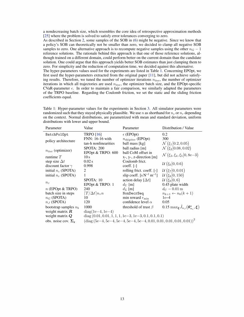
a nondecreasing batch size, which resembles the core idea of retrospective approximation methods[25] where the problem is solved to satisfy error tolerances converging to zero.As described in Section 2, some samples of the SOB in (6) might be negative. Since we know thata policy’s SOB can theoretically not be smaller than zero, we decided to clamp all negative SOBsamples to zero. One alternative approach is to recompute negative samples using the other nG − 1reference solutions. The rationale behind this approach is that one of those reference solutions, al-though trained on a different domain, could perform better on the current domain than the candidatesolution. One could argue that this approach yields better SOB estimates than just clamping them tozero. For simplicity and the reduction of computation time, we decided against this alternative.The hyper-parameters values used for the experiments are listed in Table 1. Concerning EPOpt, wefirst used the hyper-parameters extracted from the original paper [11], but did not achieve satisfy-ing results. Therefore, we tuned the number of optimizer iterations niter, the number of optimizeriterations in which all trajectories are used niter, the optimizer batch size, and the EPOpt-specificCVaR-parameter ε. In order to maintain a fair comparison, we similarly adapted the parametersof the TRPO baseline. Regarding the Coulomb friction, we set the static and the sliding frictioncoefficients equal.

Table 1: Hyper-parameter values for the experiments in Section 3. All simulator parameters wererandomized such that they stayed physically plausible. We use n as shorthand for nc or nr dependingon the context. Normal distributions, are parametrized with mean and standard deviation, uniformdistributions with lower and upper bound.

Parameter Value Parameter Distribution / Value

BatchPolOpt TRPO [16] ε (EPOpt) 0.2

policy architecture FNN: 16-16 with nskipiter (EPOpt) 300tan-h nonlinearities ball mass [kg] N

(ξ1∣∣0.2, 0.05

)niter (optimizer) SPOTA: 200 ball radius [m] N

(ξ2∣∣0.08, 0.02

)EPOpt & TRPO: 600 ball CoM offset in N

(ξ3, ξ4, ξ5

∣∣0, 8e−3)

runtime T 10 s x-, y-, z-direction [m]step size ∆t 0.02 s Coulomb frict. U

(ξ6∣∣0, 0.6)discount factor γ 0.998 coeff. [-]

initial nc (SPOTA) 2 rolling frict. coeff. [-] U(ξ7∣∣0, 0.01

)initial nr (SPOTA) 1 slip coeff. [s N−1 m−1] U

(ξ8∣∣0, 150

)nτ

SPOTA: 10 action delay [∆t] U(ξ9∣∣0, 6)

EPOpt & TRPO: 1 dU [m] 0.45 plate widthn (EPOpt & TRPO) 240 dL [m] dU − 0.01 mbatch size in steps dT/∆tenτn NonDecrSeq nk+1 ← n0(k + 1)nG (SPOTA) 10 min reward rmin 1e−4nJ (SPOTA) 120 confidence level α 0.05bootstrap samples nb 1000 threshold of trust β 0.15 maxξ JnJ

(θ?nc , ξ

)weight matrixR diag(1e−4, 1e−4)weight matrixQ diag (0.01, 0.01, 1, 1, 1, 1e−3, 1e−3, 0.1, 0.1, 0.1)

obs. noise cov. Σε (diag (5e−4, 5e−4, 5e−4, 5e−4, 5e−4, 0.01, 0.01, 0.01, 0.01, 0.01))2

13

D Supplementary Results of Experiment 3In experiment 3, we investigated to what extent SPOTA, EPOpt, TRPO, and LQR policies are ableto maintain their performance when evaluated using a different physics engine. Figure 6 displaysthe full cross-evaluation between Vortex and Bullet, i.e., the extended version of Figure 4. It canbe seen from the figures that policies trained using domain randomization generalize better to theother physics engine. In particular the SPOTA policy is able to maintain the performance level of theLQR controller, which’s parameters are invariant to the physics engine. Regarding the relatively lowperformance of the EPOpt policy, we want to add that it is common for this algorithm to yield lowerrewards for the nominal domain parameters, but to be robust against variations of these parameters(not depicted in Figure 6). Interestingly, the evaluation in Vortex yields notably better results. Oneexplanation for that could be that, despite using identical physics parameter values, we found thatthe simulation in Bullet appears to have less friction. Additional videos are provided at https://www.ias.informatik.tu-darmstadt.de/Team/FabioMuratore.

(a) Trained in Vortex, tested in Vortex (b) Trained in Vortex, tested in Bullet

(c) Trained in Bullet, tested in Vortex (d) Trained in Bullet, tested in Bullet

Figure 6: Cross-evaluation of SPOTA, EPOpt TRPO, and LQR policies trained in Vortex and thentested in Bullet. The simulators were set up to maximize the similarity between the physics enginesas much as possible. Moreover, the simulator parameters used for evaluating are the same as usedfor determining the LQR and TRPO policy, and equal to the nominal parameters for the SPOTA aswell as EPOpt procedure.

14