Does Year Round Schooling Affect the Outcome and … · Does Year Round Schooling Affect the...

Journal of Educational Research & Policy StudiesSpring 2010, Vol. 10, No. 1, pp. 79 - 97

79

Does Year Round Schooling Affect the Outcome and Growth of California’s API Scores?

Amery D. WuUniversity of British Columbia

Jake E. StoneSimon Fraser University

This paper examined whether year round schooling (YRS) in California had an effect upon the outcome and growth of schools’ Academic Performance Index (API) scores. While many previous studies had examined the connection between YRS and academic achievement, most had lacked the statistical rigour required to provide reliable interpretations. As a response, this study used data collected from 4,569 schools over six years and two integrated and more sophisticated statistical techniques – mixed analysis of covariance and latent growth model. Results showed that YRS did not affect either the outcome or the growth of API scores.

This paper examined whether year round schooling (YRS) in California had an effect upon the outcome and growth of schools’ Academic Performance Index (API) scores. Year Round Schooling refers to a school calendar that moves away from the traditional three semesters with a long summer break to shorter semesters interspersed with more but shorter holidays. Records of YRS calendars date back to the early twentieth century (Glines, 1996) with many reasons given for the creation of such calendars including helping immigrants learn English, creating more classroom space, improving learning, and meeting the needs of “laggards.” The depression and Second World War brought a pressure for conformity that ended most experiments in YRS, but by the late sixties, interest had been revived with a steady move of schools to the year round schedule in a number of states across America with various types of YRS calendar being implemented (Glines, 1996).

In California, there are a number of different calendars for YRS. Three typical calendars are 30/15 (i.e., 30 days of school followed by 15 days of holiday), 60/20 and 90/30. These schedules do not affect the total number of days spent in school in a year (California Department of Education, 2008). The Concept Six schedule, however, has more hours in a school day but just 163 days in a school year. Most year round schools

80

Wu and Stone

in California are multi-track, meaning that while some students are on break, others are still in school, which allows the capacity of a school to increase by between 25 and 50 percent (Orellana & Thorne, 1998).

The debate on the desirability of YRS is ongoing. There are a number of reasons cited for switching to a year round schedule, the most common of which are avoiding the burn out that children and teachers suffer through long semesters, and improving retention of academic learning as students do not forget what they have learned after a long summer break (Warrick-Harris, 1995). Other positive factors claimed for YRS include reducing discipline problems, improving attendance, providing more opportunity for intersession remedial classes, reducing stress, and allowing families to vacation out of peak season (Glines, 1996). There are also administrative advantages for a YRS calendar as multi-track systems expand the capacity of a school, and thus alleviate over-crowding and reducing construction and maintenance costs (Orellana & Thorne, 1998).

Criticisms of year round school include the problems entailed in managing the transition to a year round schedule, families having different schedules for older and younger children if the high school is on a traditional schedule, and the difficulty of motivating children to study in summer and hot classrooms that lack air conditioning (Glines, 1996). Multi-track year round schooling (MT-YRS) faces even more criticism as students miss out on school events and school programs that are not available on their particular track due to lack of resources. Mitchell and Mitchell (2005) provided evidence for social and ethnic segregation between tracks with academic performance varying from track to track in the same school.

The move towards MT-YRS in California can be attributed to rapid growth in school age population densities, especially in poorer immigrant communities. In the 1990s, California’s Year-Round School Grant Program encouraged school districts to move towards a MT-YRS system and by 2000, 25% of Californian school children attended year round schools, almost all of which were multi-track (Mitchell & Mitchell, 2005).

With such a large proportion of school children in MT-YRS, it is important that clear assessments can be made of its efficacy. As we saw in the description above, there are a broad number of areas in which MT-YRS influences education. However, as American educational institutions increasingly emphasize academic accountability, it is not surprising that many studies of YRS have focused upon this issue.

Palmer and Bemis (1999) reviewed 75 analyses of student achievement in YRS and found that 42 did not reveal a significant effect on achievement for students, while 27 indicated significant positive effects. A review by Zykowski, Mitchell, Hough, and Gavin (1991) concluded no difference between YRS and traditional schools. The North Carolina Department of Education used a matched sample of year-round and traditional public schools during the years 1997 and 1998, and did not determine there to be any difference in academic performance (Kirk, 2000), while Kneese (2000) reviewed thirty studies of YRS that took place in the 1990s and concluded that “there is an effective maintenance and improvement of the overall academic performance of students participating in a year-round education program” (p. 4). Shields and Oberg (2000) summarized the literature as follows:

Taken together, the literature suggests that YRS has, at worst, no impact on student

YRS Performance and Growth

81

academic performance and, at best, may be associated with gains. This seems particularly true for students in “at-risk” groups. Although some of the gains are not particularly meaningful, others are statistically significant. (p. 79)

While such a conclusion may be merited, the methodology used by many of the studies on YRS has left a little more wriggle room for interpretation than might be absolutely necessary. There are many factors that influence students’ performance and can confound with the effect of a YRS schedule. Social economic status (SES), for example, is a well-known factor affecting student performance (Jimerson, Egeland, & Teo, 1999; Lee & Burkam, 2002), and once SES has been accounted for in a regression analysis, the effect of other variables on performance typically diminishes (Betts, Rueben, & Danenberg, 2000). As Mitchell (2002) observed, many MT-YRS schools cater to students at the lower end of the SES spectrum with a proportion of English language learners that is also higher than in single-track traditional calendar schools, yet this is not always taken into account. Among the 20 inferential studies in the 1990s reviewed by Kneese (2000), only three studies used comparison groups and matched explicitly for SES. This could lead to possible misinterpretation of findings especially when YRS is compared to traditional calendar schools without taking the different SES profiles into account. Many comparisons between schools have been approximate at best. A review of 39 YRS studies by Cooper, Valentine, Charlton, and Melson (2003) found that 59% made no attempt to match students other than by comparing similar schools in similar neighbourhoods.

Furthermore, many studies of YRS do not rule out other possible explanations for the difference in achievement between YRS and non-YRS schools. Among the 20 inferential studies reviewed by Kneese’s (2000) research synthesis, only two used analysis of covariance (ANCOVA) and two used multiple regression to control for the effects of potential covariates. Eight simply used t-tests and seven used analysis of variance (ANOVA) to see if there were significant differences between groups. Neither of these methods of analysis examined whether significant differences between groups were attributable to factors other than school calendars.

Grooms and Smothermann (2003) reviewed the progress of single track YRS in thirteen school districts in Kentucky based on the California Test of Basic Skills (CTBS) composite scores. The results for YRS schools were shown to have exceeded the CTBS National Standard in 1997-1998 and 2001-2002 for both reading and mathematics. Furthermore, the results were better in 2001-2002 than 1997-1998. While this finding certainly shined a positive light upon YRS, it also leaves a few methodological questions to be answered as this report neither had a comparison group (such as non-YRS school districts), nor did it consider other possibly confounding covariates. This well publicized study did not provide any inferential statistics to demonstrate that the claimed improvement between the two testing times was not a result of chance capitalization.

Another drawback in the methodology adopted in the existing literature was the appropriateness of the design and statistical techniques used to investigate growth difference between YRS and non-YRS calendars. If data were collected through within-subject design (same study unit repeatedly measured), the independent sample

82

Wu and Stone

t-test, ANOVA, or even ANCOVA, which are only appropriate for cross-sectional data, could be flawed because the assumption of “independence” and “equal variances” underlying these techniques may be violated.

In addition, the methodology literature has long documented the potential problems of using difference scores between two waves of data with unequal variances and stressed the necessity of using at least three waves of data to study growth (e.g., Cronbach & Furby, 1970; Rogosa, 1980; Rogosa, Brandt, & Zimowski, 1982). To properly investigate growth across multiple observations, the methodology literature has recommended more integrated and advanced statistical techniques such as mixed design analysis of variance (Mixed ANOVA), multilevel modelling (MLM; a.k.a., hierarchical linear model, HLM), or structural equation modelling (SEM), which are capable of taking into account the dependence among multiple measures (Bryk & Raudenbush, 1992; Duncan, Duncan, Strycker, Li, & Alpert, 1999; Francis, Fletcher, Stuebing, Davidson, & Thompson, 1991).

Previous studies have often used a piece-meal analytical approach – studying the change in pairs of scores between two consecutive years (e.g., Grooms & Smothermann, 2003). Few, if any, of the studies that claimed to study growth trends included three or more waves of data and used appropriate statistical techniques. Consequently, the extant literature has not appropriately investigated the growth difference between YRS and non-YRS schools, or what other variables may be attributed to schools’ academic growth.

Another crucial but often-neglected measurement issue in studying growth was the use of different measures across time. When different measures are used across repeated measures, the measurement invariance requirement might be violated. Measurement invariance entails that the same outcome has been measured and measured on the same metric (Wu, Li, & Zumbo, 2007). If different tests and/or different metrics (e.g., total score) were used across time, different outcomes may have been measured and quantified on different metrics. As a result, the growth study comparing scores across time might not be meaningful. For example, different tests were used to compose the API score. Tests included in 2000 may be more difficult than those in 2001, resulting in a spurious growth that was only a reflection of the test difficulty. When different tests are used, some statistical techniques such as using ranked data, which is metric free, should complement metric data to examine whether the growth effect found in the metric data is merely a result of measurement artifact (Lloyd & Zumbo, in press).

In summary, the reservations about research methodology that we expressed above are very much echoes of similar sentiments expressed by Palmer and Bemis (1999), who noted that many studies of YRS spanned only one year with several comparing a single year-round school to a traditional school with similar student demographics. Furthermore, many studies did not conduct inferential statistical analysis, and many of those that did conduct such an analysis failed to provide key information. Cooper et al. (2003) concluded their review of the research on YRS by saying:

Perhaps the clearest conclusion to be drawn from this synthesis is that a truly credible study of modified calendar effects has yet to be conducted. It would be difficult to argue with policymakers who choose to ignore the existent database because they feel that the research designs have been simply too flawed to be trusted. (p. 43)


83

Even though a body of research on YRS has been documented, and there is a general consensus that YRS had no effect or a small positive effect on student performance, the methodology of many studies had left copious room for more rigorous verification. Furthermore, no previous study had examined the growth trajectories of school performance in YRS compared to traditional school calendars. The purpose of this study, therefore, was to use six waves of API data from the State of California to ask the following questions: 1) Does YRS have an effect upon elementary schools’ API scores when pre-existing differences in performance and demographic variables are taken into account? 2) Does YRS have an effect upon elementary schools’ growth in API scores when pre-existing differences in performance and demographic variables are taken into account?

Method

Data

California’s Public Schools Accountability Act (1999) and consequent detailed data collection has given today’s researchers an opportunity to fill in some of the methodological and statistical gaps in studies of YRS in a way that would have been so much harder a decade ago.

Our dataset was the Academic Performance Index Documentation, which consisted of demographic and performance data collected annually from every school under the auspices of the California Department of Education. This study used six data sets spanning the years 2000 to 2005.

Outcome measure – API. The API is an index derived from a series of academic tests of performance administered under California’s Standardized Testing and Reporting (STAR) Program since 1999. Prior to 2003, the Stanford 9 (Harcourt Educational Measurement, 1996), a nationally-normed test was administered to California public school students in grades 2 through 11. From 2003, the California Standards Test, which was developed by California Department of Education to be aligned more closely with the school curriculum, was used in its stead. The API for a school was calculated each year by collecting the students individual test scores, weighting the score for prescribed performance bands and then weighting for subject area such as reading or mathematics. All API scores were scaled to range from 0 to 1000. Readers can refer to California Department of Education (2001; 2006) for a clear and detailed explanation of API calculations.

This study used the API base score datasets rather than the growth score datasets. The scores in the growth dataset were already adjusted for comparison between two consecutive years so as to study year on year growth. To study the growth over the course of six years, this study required base scores without pair-wise statistical adjustment.

YRS measure. Each year, schools in the API datasets were denoted as a YRS school or a traditional calendar school. Our dataset included the 526 YRS elementary schools that had maintained their YRS schedule through the six years and the 4,043 elementary schools that had never been on a YRS schedule through the same period (never = 0, always = 1).

84

Wu and Stone

Covariates. This study included a broad number of covariates based upon what was available in the dataset, previous empirical findings, and existing theories pertaining to the factors that affect schools’ academic performance. We also conducted our own preliminary regression analyses to identify potential covariates. Because the covariates were available for each year of API data and remained consistent across six waves, with the exception of API score in the year 2000, we used a 6-year average score for each covariate. Below is the descriptions of these covariates.

The baseline API (year 2000) was treated as the pre-existing difference in performance. This was treated as a covariate in our mixed ANCOVA analysis. Note that the API 2000 score was used as the first wave data in our SEM model rather than a covariate (discussed in the Results section). The number of students tested (# of Students Tested, M = 363.03) at each school, which we referred to be an approximation of school size. The level of parents’ education (Parents’ Education, M = 2.78) was a measure collected on a voluntary basis from parents at each school that was aggregated into a school-level index ranging from one to five (not high school graduate = 1, high school graduate = 2, some college = 3, college graduate = 4, and graduate school = 5). The number of socio-economically disadvantaged students is calculated by the California Department of Education based upon the students eligible for free school meals. We converted this to a percentage and used it as an indicator of Social Economic Status (SES, M = 51.88). The percentage of students in each school who were identified as English Language Learners (% ESL Students, M = 25.53). Seven variables denoting ethnicity, which included the percentage of students who were African American (M = 7.81), American Indian (M = 1.28), Asian (M = 8.03), Filipino (M = 2.29), Hispanic (M = 40.52), Pacific Islanders (M = 0.63), and White (M = 38.35).

Results

To answer the research questions, this study adopted two different but compatible statistical methods. The first was the more conventional technique of “mixed design ANCOVA” and the second study was a “latent growth model” using a structural equation modeling technique. The employment of two methods examined whether the findings of one study would verify those of the other so that possible spurious conclusions due to methods could be ruled out. For each study, the analysis was conducted first without inclusion of any covariates and then with all the covariates. Also, the two analyses with inclusion of covariates were repeated on the ranked data to examine whether lack of measurement invariance was a possible threat to the credibility of the findings.

Study One: Mixed Design ANCOVA

The mixed design undertook the rationale of a typical quasi-experiment, where the independent variable YRS functioned as a treatment variable – a between-subject variable, and the five repeated measures of the API (2001-2005) functioned as the within-subject variable. Hence, the “mixed design” referred to the employment of both


85

a 2-level between subject variable (YRS and non-YRS) and 5-level within subject variable (years 2001-2005), entailing a 2 x 5 mixed ANOVA analysis. Because there was no random assignment of the treatments (i.e., random assignment of YRS calendar to schools), the potential variables that might have caused the pre-existing differences in the API performances were incorporated as covariates so that their confounding effects could be partialled out; hence a 2 x 5 mixed ANCOVA. These covariates included the first measure of API (i.e., baseline measure in year 2000), SES, # of Students Tested, Parent Education, % ESL Students, and the seven Ethnicity variables.

Table 1 compares the descriptive statistics of the six repeated measures of the API scores categorized by the YRS variable. It appears that, for both groups, API scores grew steadily over the studied years with schools on a YRS schedule starting with a poorer performance, a smaller variation, and a consistent lag behind those on a traditional calendar.

Table 1Descriptive Statistics of API Scores

Note. The API 2000 score was used as the baseline covariate.

Results without covariates. Because the current data violated the sphericity assumption for mixed ANOVA, Mauchly’s W = 0.204, χ2(9, N = 4,569) = 7,247.88, p < 0.001, Greenhouse-Geisser Epsilon = 0.516 (< 0.75, the suggested cut-off for violation of the sphericity assumption). Thus, the corrected Greenhouse-Geisser F test was reported for test of growth effect (i.e., within-subject effect), F(2.07, 9434.52) = 3,016.85, p < 0.001, Partial η2 = 0.398. This indicates that there was at least one true difference between a pair of API scores over two tested years.

Test of YRS effect (i.e., between-subject effect) showed that there was a significant group difference in the API scores, F(1, 4567) = 413.19, p < 0.001, Partial η2 = 0.083. This indicates that the mean of the traditional schools across five years (M = 739.19) was significant higher than that of the YRS schools (M = 651.53). There was also a significant “growth by YRS” interaction effect, F(2.07, 9434.52) = 186.84, p < 0.001, Partial η2 = 0.039. This indicates that the growth effect was dependent on whether a school was on a YRS calendar. In other words, the API growth effects were different between traditional and YRS schools.

The second and third columns of Table 2 summarize the interaction effect by tabulating the yearly API means predicted by the mixed ANOVA analysis without

YRSPerformance&Growth24

Table1

DescriptiveStatisticsofAPIScores

2000 2001 2002 2003 2004 2005

M NeverYRS 693.34 709.56 718.83 747.99 750.83 768.72

AlwaysYRS 595.97 595.97 628.30 667.69 675.66 690.02

Overall 677.79 696.49 708.41 738.75 742.18 759.66

SD NeverYRS 124.77 112.97 100.77 93.82 90.50 88.97

AlwaysYRS 109.50 96.79 78.92 70.47 66.22 66.05

Overall 130.43 116.98 102.65 94.95 91.25 90.20

Note.TheAPI2000scorewasusedasthebaselinecovariate.

86

Wu and Stone

the covariates. The profile plot on the left part of Figure 1 depicts the visual summary of the results. It shows that although both types of schools’ performance had been improving, non-YRS schools performed consistently better than YRS schools over the five-year period. Also, the “growth by YRS” interaction effect was indicated by the nonparallel lines, which show that the yearly difference between YRS and non-YRS schools was decreasing.

Table 2 Predicted Yearly API Means by Mixed ANOVA vs. Mixed ANCOVA

Results with the covariates. Would the growth effect, YRS effect, and the interaction effect remain significant if the covariates were brought into the analysis? The same mixed ANOVA analysis was conducted, however, this time the covariates were included (hence, mixed ANCOVA). Note that not only the main effects of covariates but also the “growth by covariate” interaction effects were all partialled out because the purpose was to covariate out as many of the pre-existing differences as possible1. Again, because the sphericity assumption was violated, Mauchly’s W = 0.470, χ2(9, N = 4,569) = 3,437.43, p < 0.001, Greenhouse-Geisser Epsilon = 0.700 (< 0.75). Thus, the corrected Greenhouse-Geisser F test was reported for test of growth effect, F(2.80, 12748.02) = 7.394, p < 0.001, Partial η2 = 0.002. This indicates that there was a small true growth during the studied period. Post-hoc LSD tests show that all the API scores were significantly higher than those of the previous years.

Test of YRS effect showed, once the effects of all the covariates were controlled for, the significant group difference in the API score averaged across five years disappeared, F(1, 4555) = 3.651, p = 0.056. The effect size partial η2 dropped from 0.083 to 0.001 from the model without the covariates to that with the covariates.

This indicates that the estimated mean of the traditional schools (M = 728.76) was no longer significantly higher than that of the YRS schools (M = 731.55). Although there was also a significant “growth by YRS” interaction effect, F(2.80, 12748.02) =

1 The within-by-between interaction is the default in SPSS mixed models, and is automatically calculated and outputted.


Table2

PredictedYearlyAPIMeansbyMixedANOVAvs.MixedANCOVA

MixedANOVA MixedANCOVA

Year Never

YRS

Always

YRS

Marginal

Never

YRS

Always

YRS

Marginal

2001 709.56 595.97 652.77 696.16 698.96 697.56

2002 718.83 628.30 673.56 707.91 712.22 710.06

2003 747.99 667.69 707.84 738.21 742.89 740.55

2004 750.83 675.66 713.25 741.72 745.68 743.70

2005 768.72 690.02 729.37 759.87 758.00 758.94

Marginal 739.19 651.53 691.13 728.78 731.55 730.16


87

Figure 1. Profile Plots for Mixed A

NO

VA vs. M

ixed AN

CO

VA.

5.677, p < 0.001, the effect size Partial η2 was very trivial at 0.001, a substantial drop from 0.039 for the model without the covariates.

The fifth and sixth columns of Table 2 summarize the interaction effect by tabulating the yearly API means predicted by the mixed ANCOVA. One can see that the yearly gaps between the non-YRS and YRS schools substantially closed after the inclusion of the covariates. The profile plot on the right part of Figure 1 summarizes the results. It shows that non-YRS schools’ performance was almost identical to YRS schools over the five-year period, and the interaction effect was hard to visualize. Note that because the main effects of the covariates and the interaction effects of “growth by covariates” were not the core interest of this study, they were not interpreted. Interested readers can findthem in the Appendix.

To examine the possibility of lack of measurement invariance across the six API measures, and its effect on the growth comparison, we conducted the identical mixed ANCOVA, but this time on the ranked data to

YRSPerform

ance&Grow

th30

88

Wu and Stone

examine whether the previous results could be verified. The 4,569 schools were ranked by their API score for each year. The results showed that the API rank growth effect was significant, F(2.75, 12532.44) = 21.247, p < 0.001, Partial η2 = 0.001. Test of YRS effect was not significant, F(1, 4555) = 0.162, p = 0.688, the partial η2 = 0.001. Although there was also a significant “growth by YRS” interaction effect, F(2.75, 12534.44) = 5.508, p < 0.001, the effect size Partial η2 was trivial. The results were identical to those based on raw API scores indicating that the findings on raw API scores were unlikely to be a consequence of measurement artifact.

Study Two: Latent Growth Model Using Structural Equation Model

The latent growth model depicted the observed growth trajectories of schools. The advantages of latent growth model using the SEM technique were that all the research questions could be answered in one single model, and the fit of the specified model to the given data could be computed (Muthén, 2004). Figure 2 displays the observed trajectories of the API measures over the six years (2000-2005). Each line in Figure 2 represents the trajectory of a school. Figure 2 also juxtaposes the trajectories of YRS and non-YRS schools. On the left, the YRS trajectories show a relatively lower start in the year 2000, but a relatively faster growth rate, and a relatively smaller variation compared to the trajectories of non-YRS schools on the right.

Many of the SEM software packages are capable of handling latent growth models. This study used Mplus, a very user-friendly and comprehensive statistical package (Muthén & Muthén, 1998-2006). The SEM technique was used to create two latent growth variables (i.e., unobserved variables) in order to represent the growth trend observed from the trajectories: the initial API performance and growth rate. The following description gives a conceptual account of latent growth models tailored for the present research purposes, a detailed description can be found in Duncan, Duncan, Strycker, Li, and Alpert (1999), Muthén (2004), and Muthén and Muthén (1998-2006).

Figure 3 delineates a latent growth model tailored to answer our research questions. The two latent growth variables were represented by the two ovals, which were created by summarizing the growth trend shown by the six observed measures of API. For each individual school, a latent initial performance and a latent growth rate were estimated; the means and variances of the estimated latent initial performance and growth rate hence can be calculated and predicted.

The initial performance variable was a random variable representing the starting performance of each school in the year 2000. It is the intercept, estimated API score at time zero (year 2000), of the linear trajectory for each school. The loadings (weights) of the latent initial performance on the six observed API measures were fixed to be one so as to indicate the intercepts at time zero (2000 baseline) for each school. The latentgrowth rate variable was a random variable representing the linear growth rate of each school. It is the slope, estimated yearly change of API score, of the linear trajectory foreach school. The loadings (weights) of the growth rate variables on the six observed API were fixed at 0, 1, 2, 3, 4, and 5 to indicate a constant linear growth pattern for each school.


89

Figure 2. Observed G

rowth Trajectories by Y

RS.

In this study, the initial performance was predicted by YRS indicated by the arrow going from the YRS variable to the latent initial performance. This arrow represents the unique contribution of YRS to the latent initial performance because the confounding effects were partialled out by including the covariates in the prediction, indicated by the arrow going from the covariates to the initial performance. Likewise, the arrow going from YRS to the latent growth rate indicates the unique effect of YRS on the latentgrowth rate. Note that in addition to the demographic covariates, the latent initial performance was added as a baseline covariate analogous to the observed API 2000 in the mixed ANCOVA analysis. The arrow going from the latent initial performanceto the latent growth rate indicates this baseline covariate effect. In short, the two latent growth factors, initial performance and growth rate, were treated separately as the dependent variables, and predicted by the YRS variable while all the covariate effects were partialled out.

YRSPerform

ance&Grow

th31

90

Wu and Stone

Figure 3. Latent Growth Model with Covariates.

Results of latent growth model. The fit indices shows that the model specified as in Figure 3 fit the data well2. The CFI = 0.935, TLI = 0.912, RMSEA = 0.130, and SRMR = 0.027. The R-squared values for the six observed API scores were 0.957, 0.978, 0.968, 0.954, 0.974, and 0.949. The R-squared values for the latent initial performance and growth rate were 0.855 and 0.692 respectively.

The mean of the latent initial performance was estimated at 679.73 indicating the average starting performance for all schools in year 2000. Table 3 reports the results of prediction of the latent initial performance by YRS. Controlling for the demographic covariates; the YRS school started 10.54 points lower, which is significantly lower than the non-YRS schools. Although the covariates were not the core interests of this study, their effects were also reported in Table 3.

2 In broad strokes, CFI and TLI ≥ 0.90, RMSEA≤ 0.08, and SRMR ≤ 0.05 are considered as good fit.



91

Table 3Prediction of API Initial Performance

Note. *p < 0.05; **p < 0.01.

The mean of the latent growth rate was estimated at 16.16 indicating the average yearly improvement over the five intervals from 2000 to 2005. Table 4 reports the prediction of the latent growth rate by YRS. Remember that, the latent initial API performance was added as a covariate in addition to the demographic variables. Controlling for all the covariates, the YRS schools did not improve faster or slower than the non-YRS schools. The yearly growth difference 0.30 (a.k.a., slope, the partial regression coefficient, or b-weight for YRS) was not significantly different from zero. Although the covariates were not the core interest of this study, their effects were also reported in Table 4.

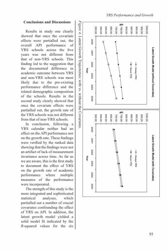
The second and third columns of Table 5 show the predicted yearly API means categorized by YRS and non-YRS without the covariates. The last two columns show the corresponding predicted means with the covariates included. The differences in the API score between YRS and non-YRS schools were substantially reduced once the covariates were included. Figure 4 summarizes the predicted trajectories indicated by the means in Table 5. The predicted trajectory on the left shows, without the covariates, the YRS started substantially lower than the non-YRS schools, but progressed faster than non-YRS schools. The trajectory on the right shows that once the covariate effects were partialled out, the difference in growth rate disappeared despite a small difference in the initial API performance. The change in growth trend as a result of including covariates was identical to that found by mixed ANCOVA in study one.

To examine the possibility of lack of measurement invariance across the six API measures and its effect on the latent growth model, we conducted the identical analysis, but this time on the ranked data to examine whether the previous results could be verified. The fit indices show that the model fit the ranked data very well. The CFI = 0.976, TLI = 0.968, RMSEA = 0.078, and SRMR = 0.007. The R-squared values forthe six observed API scores were 0.969, 0.978, 0.968, 0.967, 0.973, and 0.956. The R-squared values for the latent performance and growth rate were 0.861 and 0.207 respectively.

Predictors b-weight SE Z p YRS -10.54 2.73 -3.86 *SES (Disadvantaged) -1.37 0.07 -20.31 **# of students tested 0.01 0.01 0.97Parents' Education 51.45 2.46 20.89 **% ESL students -0.85 0.08 -11.17 *% American African students 0.23 0.39 0.59% American Indian students 0.15 0.43 0.34% Asian students 2.45 0.39 6.37 *% Filipino students 2.11 0.42 4.81 *% Hispanic students 1.02 0.38 2.70 *

92

Wu and Stone

Table 4Prediction of Growth Rate

Note. *p < 0.05; **p < 0.01.

Table 5Predicted Yearly API Means by Latent Growth Model: with vs. without Covariates

Controlling for the covariates, the YRS schools were ranked a significant 93 places lower than the non-YRS schools in the beginning year of 2000. However, controlling for all the covariates, the YRS schools did not improve faster or slower than the non-YRS schools, yearly growth difference in rank (1.8), was not significantly different from zero. The results were identical to those based on raw API scores indicating the findings on raw API scores were unlikely to be a consequence of measurement artifact.


Table5

PredictedYearlyAPIMeansbyLatentGrowthModel:withvs.withoutCovariates

WithoutCovariates WithCovariates

Year NeverYRS AlwaysYRS NeverYRS AlwaysYRS

2000 693.73 572.29 679.74 669.20

2001 707.75 598.04 695.89 685.36

2002 721.77 623.80 712.05 701.52

2003 735.79 649.55 728.21 717.68

2004 749.81 675.30 744.37 733.84

2005 763.83 701.06 760.53 749.99


Table4

PredictionofGrowthRate

Predictors bweight SE Z p

YRS 0.30 0.42 0.71

InitialPerformance 0.12 0.00 46.04 **

SES(Disadvantaged) 0.03 0.01 2.66 *

#ofstudentstested 0.00 0.00 3.16 *

Parents'Education 8.14 0.40 20.31 **

%ESLstudents 0.04 0.01 3.12 *

%AmericanAfricanstudents 0.35 0.06 5.81 *

%AmericanIndianstudents 0.26 0.07 3.89 *

%Asianstudents 0.50 0.06 8.38 *

%Filipinostudents 0.38 0.07 5.85 *

%Hispanicstudents 0.43 0.06 7.39 *

%PacificIslanders 0.00 0.12 0.03

%Whitestudents 0.40 0.06 6.70 *

Note.*p<0.05.**p<0.01.


93

Conclusions and Discussions

Results in study one clearly showed that once the covariate effects were partialled out, the overall API performance of YRS schools across the five years was not different from that of non-YRS schools. This finding led to the suggestion that the documented difference in academic outcome between YRS and non-YRS schools was most likely due to the pre-existing performance difference and the related demographic composition of the schools. Results in the second study clearly showed that once the covariate effects were partialled out, the growth rate of the YRS schools was not different from that of non-YRS schools.

In conclusion, following a YRS calendar neither had an effect on the API performance nor on the growth rate. These findings were verified by the ranked data showing that the findings were not an artifact of lack of measurement invariance across time. As far as we are aware, this is the first study to document the effect of YRS on the growth rate of academic performance where multiple measures of the performance were incorporated.

The strength of this study is the more integrated and sophisticated statistical analyses, which partialled out a number of crucial covariates confounding the effect of YRS on API. In addition, the latent growth model yielded a solid model fit indicated by the R-squared values for the six

Figure 4. Latent Grow

th Trajectories: with vs. w

ithout the Covariates.

YRSPerform

ance&Grow

th33

94

Wu and Stone

observed API scores, which were all greater than 0.9, in addition to the other important fit indices. Using two data-analytical approaches, the mixed ANCOVA and the latent growth model, that yielded almost identical findings as shown in Figure 1 and 4, we confirmed that the findings were unlikely to be a consequence of statistical artifact. The large sample size ruled out the possibility that the statistically non-significant effect of YRS on API performance and growth was due to low statistical power.

A major caveat is that these findings cannot be construed as a general conclusion that there is no difference in educational outcomes between YRS and traditional calendar schools. While the API has proven to be a useful indicator of student and school performance, it is not the only measure and does not take into account other important educational goals such as the well being of students and teachers, learning, development of creativity or social development. The debate on YRS needs to move on from normative measures of academic achievement to other equally important comparisons of educational attainment.

The findings of this study are limited in that the API in itself is an index. As with economic indices such as the Consumer Price Index, the content and measurement standards of the index are adjusted from year to year and the assignment of weightings to different factors that contribute to the index is as much an art as it is a science. Findings based solely upon the API must be considered as an informative guide and need further verification by other samples and other outcome measures.

An often-stated advantage of year round school is that the students lose less time in fall as they regain the academic standard that slipped through the summer vacation. The API, however, does not take this difference between YRS and traditional calendar schools into account as it is based upon a single annual measurement of achievement for each domain of interest. Future research may provide additional findings as to whether the retention of learning through the summer months provides additional value that is not identified in the API data.

Furthermore, it is not yet clear whether student performance in multi-track YRS is different to single track YRS, nor is it known how different YRS schedules affect student performance. A future study should investigate how different schedules and multi-track systems influence learning both at the national level and in California where the Concept Six schedule, for example, is quite different from other MT-YRS schedules.

References

Betts, J. R., Rueben, K. S., & Danenberg, A. (2000). Equal resources, equal outcomes? The distribution of school resources and student achievement in California. San Francisco, LA: Public Policy Institute of California.

Bryk, A. S., & Raudenbush, S. W. (1992). Hierarchical linear models: Applications and data analysis methods. Newbury Park, CA: Sage.

California Department of Education. (2001). 2000 academic performance index base report: information guide. Retrieved from: http://www.cde.ca.gov/ta/ac/ap/

California Department of Education. (2006). 2005 academic performance index base report: information guide. Retrieved from http://www.cde.ca.gov/ta/ac/ap/


95

California Department of Education. (2008). Year-round education program guide – multitrack year-round education. Retrieved from http://www.cde.ca.gov/ls/fa/yr/guide.asp

Cooper, H., Valentine, J., Charlton, K., & Melson, A. (2003). The effects of modified school calendars on student achievement and on school and community attitudes. Review of Education Research, 73(1), 1-52.

Cronbach, L., & Furby, L. (1970). How we should measure ‘change’ or should we? Psychological Bulletin, 74, 68-80.

Duncan, T. E., Duncan, S. C., Strycker, L. A., Li, F., & Alpert, A. (1999). An introduction to latent variable growth curve modeling: Concepts, issues, and applications. Mahwah NJ: Lawrence Erlbaum Associates.

Francis, D. J., Fletcher, J. M., Stuebing, K. K., Davidson, K. C., & Thompson, N. M. (1991). Analysis of change: Modelling individual growth. Journal of Consulting and Clinical Psychology, 59, 27–37.

Glines, D. (1996). YRE basics: History, methods, concerns, future. In R. Fogarty (Ed.), Year round education: A collection of articles (pp. 13-28). Arlington Heights: IRI/Skylight Training and Publishing Inc.

Grooms, A., & Smothermann, R. (2003). Study of year-round education in select Kentucky school districts. Cincinnati, OH: Educational Services Institute.

Harcourt Educational Measurement. (1996). Stanford achievement test series, 9th Ed. San Antonio, TX: Harcourt Educational Measurement.

Jimerson, S., Egeland, B., & Teo, A. (1999). A longitudinal study of achievement trajectories: Factors associated with change. Journal of Educational Psychology, 91, 116-126.

Kirk, P. J. (2000). Year-round schools and achievement in North Carolina. NC: State Board of Education.Kneese, C. (2000). Year round learning: A research synthesis relating to student

achievement. San Diego, CA: National Association of Year Round Education.Lee, V., & Burkam, D. (2002). Inequality at the starting gate: Social background

differences in achievement as children begin school. Washington, DC: Economic Policy Institute.

Lloyd, J. E. V., & Zumbo, B. D. (in press). The non-parametric difference score: A workable solution for analysing two-wave change when the measures themselves change across waves. Journal of Modern Applied Statistical Methods.

Mitchell, R. E. (2002). Segregation in California’s K-12 public schools: Biases in implementation, assignment, and achievement with the multi-track year-round calendar. Expert report prepared for counsels for the plaintiffs, Williams et al. v. State of California et al., Superior Court, San Francisco, California.

Mitchell, R. E., & Mitchell, D. E. (2005). Student segregation and achievement tracking in year- round schools. Teachers College Record, 107(4), 529-562.

Muthén, B. (2004). Latent variable analysis: Growth mixture modelling and related techniques for longitudinal data. In D. Kaplan (Ed.), Handbook of quantitative methodology for the social sciences (pp. 345-368). Newbury Park, CA: Sage Publications.

Muthén, L., & Muthén, B. (1998-2006). Mplus user’s guide. Los Angeles: Author.

96

Wu and Stone

Orellana, M., & Thorne, B. (1998). Year-round schools and the politics of time. Anthropology and Education Quarterly, 29(4), 446-472.

Palmer, E. A., & Bemis, A. E. (1999). Year-round education. (Just in time research: Children, Youth, & families). Retrieved from www.extension.umn.edu/distribution/familydevelopment/09

Public Schools Accountability Act, California State. (1999). Rogosa, D. R. (1980). Comparisons of some procedures for analyzing longitudinal

panel data. Journal of Economics and Business, 32, 136-151.Rogosa, D. R., Brandt, D., & Zimowski, M. (1982). A growth curve approach to the

measurement of change. Psychological Bulletin, 92, 726-748.Shields, C. M., & Oberg, S. L. (2000). Year-round schooling: promises and pitfalls.

Lanham, MD: Scarecrow Press. Warrick-Harris, E. (1995). Year-round school: The best thing since sliced bread.

Childhood Education, 71, 282-287.Wu, A. D., Li, Z., & Zumbo, B. D. (2007, February). Decoding the meaning of factorial

invariance and updating the practice of multi-group confirmatory factor analysis: A demonstration with TIMSS data. Practical Assessment Research & Evaluation, 12, Retrieved from http://pareonline.net/genpare.asp?wh=0&abt=12

Zykowski, J. L., Mitchell, D. E., Hough, D., & Gavin, S. E. (1991). A review of year-round education research. Riverside, CA: California Educational Research Cooperative.


97

Appendix

Covariate and Growth x Covariate Effects Partialled out in Mixed ANCOVAPredictors F p Partial η2

API2000 (Baseline) 4,880.194 0.000 0.517SES 38.980 0.000 0.008# of students tested 22.872 0.000 0.005Parents' Education 521.859 0.000 0.103% ESL students 2.117 0.146 0.000% American African students 33.386 0.000 0.007% American Indian students 24.266 0.000 0.005% Asian students 84.154 0.000 0.018% Filipino students 43.750 0.000 0.010% Hispanic students 60.874 0.000 0.013% Pacific Islanders 0.437 0.508 0.000% White students 53.012 0.000 0.012Growth x API2000 678.226 0.000 0.130Growth x SES 1.071 0.357 0.000Growth x # of students tested 2.869 0.039 0.001Growth x Parents' Education 121.837 0.000 0.026Growth x % ESL students 4.068 0.008 0.001Growth x % American African 13.343 0.000 0.003Growth x % American Indian 5.020 0.002 0.001Growth x % Asian 21.176 0.000 0.005Growth x % Filipino 9.616 0.000 0.002Growth x % Hispanic 17.074 0.000 0.004Growth x % Pacific Islander 2.052 0.109 0.000Growth x % White 14.082 0.000 0.003

Does Year Round Schooling Affect the Outcome and … · Does Year Round Schooling Affect the...

Documents

Transcript of Does Year Round Schooling Affect the Outcome and … · Does Year Round Schooling Affect the...