Does segregation matter for Latinos? - Jorge De la …Does segregation matter for Latinos? Jorge De...
30
Does segregation matter for Latinos? Jorge De la Roca * ‡ University of Southern California Ingrid Gould Ellen * § New York University Justin Steil * ¶ Massachusetts Institute of Technology This version, October 2017 Abstract: We estimate the effects of residential racial segregation on socio-economic outcomes for native-born Latino young adults over the past three decades. Using individual public use micro-data samples from the Census and a novel instrumental variable, we find that higher levels of metropolitan area segregation have negative effects on Latino young adults’ likelihood of being either employed or in school, on the likelihood of working in a professional occupation, and on income. The negative effects of segregation are somewhat larger for Latinos than for African Americans. Controlling for Latino and white exposure to neighborhood poverty, neighbors with college degrees, and industries that saw large increases in high-skill employment explains between one half and two thirds of the association between Latino-white segregation and Latino-white gaps in outcomes. Key words: racial segregation, Hispanics/Latinos, spatial inequality jel classification: j15, r23 * We thank Morgane Laouenan and Jonathan L. Rothbaum for valuable comments and discussions. We also thank Maxwell Austensen, Gerard Torrats Espinosa, and Justin Tyndall for their exceptional research assistance. ‡ Corresponding author. Sol Price School of Public Policy, University of Southern California, 650 Childs Way rgl 326, Los Angeles, ca 90089, usa (e-mail: [email protected]; website: http://jorgedelaroca.name). § Robert F. Wagner Graduate School of Public Service, New York University, 295 Lafayette Street, New York, ny 10012, (e-mail: [email protected]; website: https://wagner.nyu.edu/community/faculty/ingrid-gould-ellen). ¶ Department of Urban Studies and Planning, Massachusetts Institute of Technology, 77 Massachusetts Avenue, Room 9–515, Cambridge, ma 02139 (e-mail: [email protected]; website: https://steil.mit.edu/).
Transcript of Does segregation matter for Latinos? - Jorge De la …Does segregation matter for Latinos? Jorge De...

Does segregation matter for Latinos?
Jorge De la Roca*‡
University of Southern California
Ingrid Gould Ellen*§
New York University
Justin Steil*¶
Massachusetts Institute of Technology
This version, October 2017
Abstract: We estimate the effects of residential racial segregation onsocio-economic outcomes for native-born Latino young adults over thepast three decades. Using individual public use micro-data samplesfrom the Census and a novel instrumental variable, we find that higherlevels of metropolitan area segregation have negative effects on Latinoyoung adults’ likelihood of being either employed or in school, on thelikelihood of working in a professional occupation, and on income. Thenegative effects of segregation are somewhat larger for Latinos thanfor African Americans. Controlling for Latino and white exposure toneighborhood poverty, neighbors with college degrees, and industriesthat saw large increases in high-skill employment explains between onehalf and two thirds of the association between Latino-white segregationand Latino-white gaps in outcomes.
Key words: racial segregation, Hispanics/Latinos, spatial inequalityjel classification: j15, r23
*We thank Morgane Laouenan and Jonathan L. Rothbaum for valuable comments and discussions. We also thankMaxwell Austensen, Gerard Torrats Espinosa, and Justin Tyndall for their exceptional research assistance.
‡Corresponding author. Sol Price School of Public Policy, University of Southern California, 650 Childs Way rgl 326,Los Angeles, ca 90089, usa (e-mail: [email protected]; website: http://jorgedelaroca.name).
§Robert F. Wagner Graduate School of Public Service, New York University, 295 Lafayette Street, New York, ny 10012,(e-mail: [email protected]; website: https://wagner.nyu.edu/community/faculty/ingrid-gould-ellen).
¶Department of Urban Studies and Planning, Massachusetts Institute of Technology, 77 Massachusetts Avenue, Room9–515, Cambridge, ma 02139 (e-mail: [email protected]; website: https://steil.mit.edu/).

1. Introduction
Between 1990 and 2010, the Latino population in the United States more than doubled, from 22.4million to 50.5 million. As the Latino population has grown, levels of Latino-white residentialsegregation (as measured by the dissimilarity index) have remained relatively steady (at around0.50), while levels of Latino isolation have risen (from 0.43 in 1990 to 0.46 in 2010) (De la Roca, Ellen,and O’Regan, 2014).1 Despite this durable residential segregation, there has been little explorationof how that segregation affects the socio-economic outcomes of Latinos.
While existing research has found that black-white segregation negatively affects socio-economic outcomes for African Americans (e.g. Cutler and Glaeser, 1997, Ellen, 2000, Card andRothstein, 2007), there are reasons to expect that segregation may not have the same negativeconsequences for Latinos. For instance, research on ethnic enclaves has suggested that ethnicconcentration, in some circumstances, can improve employment outcomes by creating a marketfor ethnic goods and access to co-ethnic sources of capital (Portes and Sensenbrenner, 1993, Edin,Fredriksson, and Aslund, 2003, Cutler, Glaeser, and Vigdor, 2008). Residential segregation maystill undermine the socio-economic outcomes of Latinos, however, through the same mechanismsthat have been suggested to limit opportunities for blacks, by constraining Latinos to live inneighborhoods with less public investment, lower levels of human capital, or limited access toparticular jobs and job networks (Kain, 1968, Loury, 1977, Borjas, 1995, Lou and Song, 2017).
Thus, we examine how levels of residential segregation affect the educational and labor marketoutcomes of Latino young adults and how those effects differ from the effects of segregationon the outcomes of black young adults. To address concerns regarding within-city sorting, weexamine how metropolitan-level segregation affects the outcomes of individuals living anywherein the metropolitan area. To mitigate bias from across-city sorting, we restrict our sample tonative-born young adults and use the segregation level of the metropolitan area where they livedfive years earlier, lag our measurement of segregation by ten years, estimate longitudinal modelswith metropolitan area fixed effects, and focus on variation in effects between Latino and whiteresidents of the same metropolitan area, differencing out any residual unobserved attributes of themetropolitan area that may be related to segregation and affect outcomes. Finally, we also employinstrumental variables.
Specifically, we use a new instrument to predict Latino-white segregation, which capturesthe evenness of the distribution of single-family detached houses in relation to other types ofhousing in the metropolitan housing stock in 1970. The assumption is that the historical sepa-ration of single-family detached homes from other types of dwellings, such as attached homes ormulti-family buildings, contributes to contemporary levels of Latino metropolitan area segregationbecause Latinos are less likely to live in detached, single-family homes than other types of housing(Weicher and Thibodeau, 1988, Brueckner and Rosenthal, 2009). This instrument is more predictiveof Latino-white segregation than instruments that have been used for black-white segregation.
1Levels of black-white segregation over the same period declined somewhat (from a dissimilarity score of 0.68 to0.59) but remained high. Levels of black residential isolation also declined, but remained high (declining from 0.55 to0.46).
1

Using public-use decennial census data for 1990 and 2000 and data from the American Commu-nity Survey for 2007-2011, we examine how metropolitan area levels of segregation affect collegegraduation rates, employment rates, the likelihood of being in a professional occupation, andincome for native-born Latino and African-American young adults between the ages of 25 and 30.The estimates from longitudinal models with metropolitan area fixed effects show that segregationis negatively associated with each of the measured socio-economic outcomes of both Latino andAfrican-American young adults relative to whites.
These results, however, mask substantial heterogeneity in the link between segregation and out-comes for Latino groups of different ancestry and class status. Controlling for the heterogeneousexperiences of different Latino ancestry groups, we find that segregation has a significant negativeassociation with socio-economic outcomes for those who identify their ancestry in Mexico, SouthAmerica, Central America, the Dominican Republic, or Puerto Rico, but not for those who identifyas Cuban or of ‘another Hispanic origin.’
The instrumental variable results add a more robust causal analysis and confirm that segrega-tion has a negative effect on Latino young adults’ likelihood of being employed or in school, ontheir likelihood of working in a professional occupation, and their income. Segregation widensthe gaps in outcomes between Latinos and whites: in 2010, a one standard deviation increasein the metropolitan area level of segregation is associated with a decrease for Latinos relative towhites of 8 percentage points in college graduation rates and 15 percent in income, equivalent toa $4,219 annual income loss. The instrumental variable results also indicate that the wider gaps insocio-economic outcomes in more segregated metropolitan areas are driven in part by the fact thatwhites in those areas fare better than those in less segregated areas.
To understand why segregation has these effects, we examine potential mechanisms. We findthat the exposure of white and Latino residents to neighborhood poverty, neighbors with collegedegrees, and high-employment growth industries between 1990–2010 together explain betweenone half and two thirds of the association between segregation and white-Latino gaps in outcomes.
2. Theoretical framework and hypotheses
The effects of residential segregation are theoretically ambiguous and have been found to varysignificantly across groups and contexts. Residential segregation shapes access to neighborhoods,which in turn shape access to institutions, peers, and social networks, as well as exposure to crimeand environmental benefits and hazards (Durlauf, 2004, Bayer, Ross, and Topa, 2008, Epple andRomano, 2011, Ludwig, Sanbonmatsu, Gennetian, Adam, Duncan, Katz, Kessler, Kling, Lindau,Whitaker, and McDade, 2011, Graham, 2016). But the resources and opportunities that raciallyor ethnically homogenous neighborhoods provide are likely to vary depending on the socio-economic attributes of the group. In general, groups with greater economic or other resourcesmay benefit from segregation while those with fewer resources may be harmed.
Several studies have found that for immigrant groups with higher mean levels of human cap-ital, ethnic concentration is associated with better outcomes in employment and earnings, whilefor groups with lower mean levels of human capital, segregation is linked to lesser benefits or
2

negative effects (Borjas, 1995, Edin, Fredriksson, and Aslund, 2003, Cutler, Glaeser, and Vigdor,2008). Human capital levels have been found to shape the effects of segregation for native-bornblacks as well. For instance, increases in the proportion of college-educated African Americansin the metropolitan area reduce the negative effects of segregation on black youths’ educationalattainment (Bayer, Fang, and McMillan, 2014).
The average financial and political capital of a group also matters. Racial and ethnic groups withlower levels of financial and political capital may be less able to demand equal access to crucialmunicipal services, like school investment and community policing, to non-profit institutions thatprovide services and networks, and to private businesses that meet daily needs like child-care(Collins and Williams, 1999). Perhaps even more critically, violence tends to be disproportionatelyconcentrated in low-income neighborhoods and even indirect exposure to neighborhood violencediminishes academic performance (Sharkey, Schwartz, Ellen, and Lacoe, 2014).
Latinos in the United States have lower than average levels of education and income, andarguably less political clout given lower citizenship rates than whites, which may translate intoinferior neighborhood services and environmental amenities. Indeed, available measures of dif-ferences in neighborhood characteristics find that Latinos in more segregated metropolitan areasare exposed to fewer college educated neighbors, lower performing schools, and higher levels ofviolent crime than Latinos in less segregated cities (Steil, De la Roca, and Ellen, 2015).
There is of course, considerable variation in the socio-economic backgrounds of different Latinosub-groups in the United States. In 2010, nearly two thirds (63 percent) of the us Latino populationidentified as having Mexican ancestry, while 9 percent reported Puerto Rican, 8 percent CentralAmerican, 6 percent South American, 4 percent Cuban, 3 percent Dominican, and 8 percent ‘an-other Hispanic origin’ (United States Bureau of the Census, 2010). Mean educational attainmentvaries significantly by self-identified group of origin. For instance, 36 percent of Latinos in theUnited States who were 25 years and over and identified as having South American ancestry had acollege degree or higher in 2013 while only 20 percent of those identifying Puerto Rican origins, 14
percent of those identifying Central American origins, and 11 percent of those identifying Mexicanorigins had college degrees. There is similar heterogeneity with regard to childhood poverty. In2012, more than a third of those under 18 years of age with Puerto Rican (38 percent), CentralAmerican (36 percent), and Mexican (35 percent) origins lived below the poverty line compared to22 percent of those of Cuban descent, and 20 percent of those of South American descent (UnitedStates Bureau of the Census, 2013). This heterogeneity of Latino experiences by ancestry is likelyto contribute to variation in the effects of segregation.
While segregation’s effects may vary across groups, they are also likely to vary over time.For example, the negative effects of black-white residential segregation on black educational at-tainment and employment rates did not emerge until the economic restructuring and dramaticneighborhood change of the 1970s (Collins and Margo, 2000). There are reasons to believe thatthe effects of segregation on Latinos may differ over time as well. For instance, as the Latinopopulation in the United States has grown and Latinos have settled across a larger set of smallermetropolitan areas, the differences in neighborhood environments enjoyed by Latinos in high andlow segregation areas may have diminished.
3

3. Data and methods
To examine how metropolitan area segregation affects individual socio-economic outcomes, weuse public-use micro data gathered by the us Census and provided by ipums–usa of the Universityof Minnesota Population Center (Ruggles, Genadek, Goeken, Grover, and Sobek, 2015). We focusour analysis on data from the Decennial Censuses 5% samples in 1990 and 2000 and from theAmerican Community Survey (acs) 5-year estimates (2007-2011) to study the relationship betweenresidential segregation and socio-economic outcomes of native-born Latinos between the ages of25 and 30.2
We consider educational outcomes such as the probability of college graduation and labormarket outcomes such as the probability of working in a professional occupation, income and thelikelihood of being employed or in school. We focus on young adults because their metropolitanarea of residence is more likely to be affected by parental location choices than that of older adults.In order to most accurately estimate the level of segregation to which an individual was exposedwhile growing up, we lag our segregation measures by 10 years and use the level of segregation inthe metropolitan area in which the individual lived five years prior, for the 1990 and 2000 Census,and one year prior, for the 2007-2011 acs.3 We exclude the foreign born because the data do notprovide precise information on their year of arrival and, hence, we cannot tell how long they haveexperienced segregation.
Our sample includes individuals living in 187 Core Based Statistical Areas (cbsas) across theUnited States with a total population greater than 100,000 residents and a Latino population ofat least 5,000 residents in 2010 (see appendix A for a detailed explanation on the assignment ofindividuals in ipums to cbsas in each decade).4 Throughout the study, we use the metropolitanarea dissimilarity index from us2010, a joint project between the Russell Sage Foundation andBrown University, as our primary measure of Latino-white residential segregation.
Table 1 presents raw differences in socio-economic outcomes, pooled across 1990, 2000, and2010, by quartile of metropolitan area segregation. The upper panel shows segregation quartilesbased on the 2000 Latino-white dissimilarity index and the lower panel shows quartiles based onthe 2000 black-white dissimilarity index. Higher levels of segregation are consistently associatedwith larger gaps in every outcome between whites and blacks and between whites and Latinos.Notably, the link between segregation and racial differences in outcomes appears to be driven bothby better white outcomes and by worse black and Latino outcomes in more segregated areas.
Although these raw means by segregation quartile suggest a relationship between segrega-tion and outcomes, determining how the level of segregation shapes individual socio-economic
2Selective ethnic attrition may produce some bias in estimates of Latino educational and labor market outcomes(Duncan and Trejo, 2011); however, the acs does not allow us to control for immigrant generation or identify ethnicityother than through respondents’ self-reporting.
3We drop individuals in the armed forces and those living in group quarters, and we also estimate robustness teststhat exclude all those who recently moved across metropolitan areas.
4When looking at how metropolitan area segregation affects black young adults, our sample includes individualsliving in 184 Core Based Statistical Areas with a total population greater than 100,000 residents and a black populationof at least 5,000 residents in 2010.
4

Table 1: Relationship between segregation and outcomes, 1990–2010
College Not Professional Loggraduation idle occupation earnings
(1) (2) (3) (4)
Whites,All metropolitan areas 35.4% 89.4% 30.9% 9.94Low segregation 30.3% 87.9% 26.7% 9.81Moderate segregation 32.2% 88.9% 28.7% 9.87High segregation 33.3% 89.3% 29.6% 9.92Very high segregation 38.7% 89.9% 33.1% 10.01
Latinos,All metropolitan areas 15.9% 84.1% 18.6% 9.77Low segregation 21.1% 86.4% 21.0% 9.75Moderate segregation 16.0% 84.8% 18.6% 9.70High segregation 14.6% 84.5% 17.9% 9.73Very high segregation 16.2% 83.7% 18.7% 9.79
White-Latino gapAll metropolitan areas 19.5% 5.3% 12.3% 0.17Low segregation 9.2% 1.5% 5.8% 0.06Moderate segregation 16.2% 4.1% 10.1% 0.17High segregation 18.7% 4.8% 11.7% 0.19Very high segregation 22.5% 6.2% 14.5% 0.21
Whites,All metropolitan areas 35.4% 89.4% 30.9% 9.94Low segregation 28.4% 87.8% 26.9% 9.87Moderate segregation 32.6% 88.8% 28.7% 9.86High segregation 35.6% 90.2% 30.9% 9.94Very high segregation 37.8% 89.5% 32.4% 9.98
Blacks,All metropolitan areas 16.2% 83.5% 17.0% 9.56Low segregation 15.8% 85.5% 17.1% 9.59Moderate segregation 16.6% 85.2% 16.8% 9.54High segregation 17.4% 85.1% 18.3% 9.61Very high segregation 15.7% 82.4% 16.6% 9.55
White-black gapAll metropolitan areas 19.2% 5.9% 13.8% 0.38Low segregation 12.7% 2.3% 9.8% 0.27Moderate segregation 16.0% 3.6% 12.0% 0.32High segregation 18.1% 5.0% 12.7% 0.33Very high segregation 22.1% 7.1% 15.8% 0.43
Notes: In the top (bottom) panel, Core Based Statistical Areas are classified into quartiles—low, moderate, high andvery high—based on their 2000 Latino-white (black-white) dissimilarity index. Sample in the top (bottom) panel isrestricted to native-born whites and Latinos (blacks) between 25 and 30 years living in 187 (184) metropolitan areaswith population above 100,000 residents and more than 5,000 Latinos (blacks) in 2010. ’Not idle’ takes value one if theindividual is working or enrolled in school. Log annual income includes total income for the previous calendar yearand is available only for individuals who report positive income.
5

outcomes is intrinsically difficult because people sort into cities and neighborhoods based ontheir tastes, preferences, and unobserved resources. To address sorting across neighborhoods, wemeasure segregation at the level of the metropolitan area rather than at the level of the neigh-borhood (Cutler and Glaeser, 1997). A metropolitan area level of analysis has the added strengthof capturing metropolitan area wide restrictions on choice and of measuring how all membersof a racial or ethnic group in a metropolitan area may be affected by levels of segregation thatoperate at a higher spatial level, even those who do not live in a racially or ethnically homogenousneighborhood themselves (Chetty, Hendren, Kline, and Saez, 2014). We focus on variation in effectsacross racial or ethnic groups to difference out any unobserved characteristics of a metropolitanarea that shape economic outcomes and are correlated with segregation.
To learn how metropolitan area segregation affects Latinos, we regress an individual outcomesuch as the probability of college graduation or the likelihood of being employed or in school on ameasure of Latino metropolitan area residential segregation (e.g. Latino-white dissimilarity index).Specifically we estimate the following specification:
Yijt = α1 + β1 Segj,t−1 + β2 Segj,t−1 × Latinoij + β3 Xijt + β4 Zjt + Tt + ε ijt (1)
where Yijt represents a socio-economic outcome for individual i in metropolitan area j in decadet, Segj,t−1 is the dissimilarity index between Latinos and whites for metropolitan area j in theprevious decade t − 1, Xijt is a vector of individual level characteristics, Zjt is a vector of metropoli-tan level characteristics described below, and Tt is a decade time control. We let the coefficienton metropolitan area level of segregation—β2 in equation (1)—differ for whites and Latinos(Segj,t−1 × Latinoij). Therefore, we test whether segregation has a different association withsocio-economic outcomes for Latinos relative to its association with outcomes for whites.5 We lagsegregation to help address concerns about reverse causality and to better capture the segregationlevels present when young adults were growing up.
We include several individual variables as controls, including age indicator variables, gender,and a set of indicator variables for Latino groups of different origin (Mexicans, Puerto Ricans, Do-minicans, Cubans, Central Americans, and South Americans). As discussed above, these ancestrygroups exhibit substantial differences in levels of educational attainment, income, and presumablyunobserved traits that could explain differences in outcomes among Latinos. By including theseancestry-group indicator variables we capture a share of the variance in outcomes that can beattributed to the fact that Latinos of specific subgroups, who may be concentrated in differentmetropolitan areas, bring different backgrounds and may experience different treatment.
We also include additional time-varying metropolitan area level controls, specifically metropoli-tan area population and median household income, the fraction of the metropolitan area popula-tion that is Latino, black, Asian, foreign born, over 65 years, under 15 years, and unemployed,as well as the share of the metropolitan area workers employed in the manufacturing sector andworking in professional occupations, the share of residents with a college degree, the share of resi-dents in poverty status, and census region-year indicator variables. We interact these metropolitan
5The sum of the coefficient on segregation and the interaction of segregation with the Latino indicator variablecaptures the total effect of segregation on Latinos.
6

area controls with a Latino indicator variable to let the effects of metro area characteristics differ forLatinos as compared to whites. Again, by including all of these metropolitan area level variablesand interacting segregation with a Latino indicator variable, we test whether the level of segre-gation in a metropolitan area has a significantly different, independent effect on socio-economicoutcomes for Latinos than it does for whites.
Earlier work exploring the impacts of metropolitan segregation on individual outcomes hasonly examined a single year of data (e.g. Cutler and Glaeser, 1997). Using multiple years of dataallows us to introduce metropolitan area level fixed effects to examine how changes over time inthe level of Latino segregation in a metropolitan area are associated with changes in outcomes,while controlling for other unobserved, time-invariant metropolitan area-level factors.
To minimize both potential endogeneity from omitted variables and the reverse causality thatcould come from the gap in socio-economic outcomes between Latinos and whites itself con-tributing to metropolitan area levels of segregation, we estimate two-stage least squares models.These models address reverse causation in which a segment of the population already living in ametropolitan area might cause future segregation, but, because the instrumental variable is itselfcorrelated with segregation, their ability to fully address sorting from selection choices made bysubsequent movers is more limited (Ananat, 2011, Rosenthal and Ross, 2015). Multiple instrumen-tal variables have been developed to predict levels of black-white metropolitan area segregation,including rivers (Hoxby, 2000) and railroad tracks (Ananat, 2011), features of the natural or builtenvironment that enabled the black-white segregation that became entrenched through the rise ofJim Crow, the Great Migration, and post-war suburbanization.
These instruments, however, are not necessarily appropriate for the Latino-white segregationthat has emerged with the growth of the Latino population in the United States since 1970, giventhe different historical context. To instrument for levels of Latino-white dissimilarity from 1990
to 2010, we rely on an instrument that captures features of the historical built environment thatallowed for more segregation. Specifically, we create a variable measuring the dissimilarity indexbetween single-family detached housing and other housing types in 1970. In 1970, there were9.1 million individuals who identified as Latino in the United States, accounting for only 4.7percent of the population. In the four decades after the passage of the 1965 Immigration andNationality Act, more than 29 million immigrants from Latin America moved to the United States(Pew Research Center, 2015), and the relatively low incomes of those migrants constrained many tolive in less-expensive multi-family housing. We hypothesize that when different types of housingare ex-ante placed in separate parts of the city, more segregation is likely to result, as Latinos arelikely to disproportionately settle in multi-family or single-family attached housing because oftheir lower homeownership rates and lower average incomes (see Weicher and Thibodeau, 1988
and Brueckner and Rosenthal, 2009, for a related measure of the age of the housing stock).6
6To construct this instrument, we use the 1970 Neighborhood Change Database (ncdb) to calculate the dissimilarityindex in 1970 between single-family detached housing and all other types of housing units (single-family attacheddwellings, as well as all multi-family dwellings) for each Standard Metropolitan Statistical Area (smsa), the 1970
definition of metropolitan areas. The source units of analysis are census tracts as defined in 1970. We have data oninstruments for 142 out of the 187 cbsas in the initial sample. Those cbsas missing from the 2sls sample are generallysmaller and more recently recognized cbsas.
7

Table 2: Types of housing units by racial/ethnic group, 1980–2010
One family One family Building Building Otherdetached attached with 2 to 9 with 10+ (e.g. mobile
house house units units home, boat)
Whites,1980 60.2% 4.6% 16.2% 15.3% 3.6%1990 59.4% 6.3% 14.3% 14.5% 5.5%2000 62.7% 6.5% 12.7% 13.5% 4.7%2010 64.9% 6.9% 11.2% 13.0% 4.0%
Latinos,1980 42.9% 5.1% 24.8% 25.5% 1.7%1990 41.7% 7.0% 22.9% 24.4% 3.9%2000 42.9% 7.6% 21.8% 23.8% 3.9%2010 48.0% 6.6% 20.3% 20.9% 4.2%
Blacks,1980 39.2% 9.6% 26.9% 23.4% 0.9%1990 39.3% 10.1% 24.9% 23.0% 2.6%2000 42.5% 10.2% 23.4% 22.2% 1.8%2010 44.8% 9.8% 21.8% 21.8% 1.6%
Notes: ipums-usa data for 1990 5% sample Decennial Census, 2000 5% sample Decennial Census and acs 2007–2011.Race/ethnicity of household head is assigned to the type of housing unit. The sample for whites and Latinos isrestricted to the 142 Core Based Statistical Areas (cbsas) that are used in instrumental variable estimations, while thesample for blacks is restricted to the 147 cbsas used in analogous estimations.
In table 2, we present the share of white, Latino, and black households living in different typesof housing units by decade from 1980 to 2010. In each decade, Latinos are more likely to live inmulti-family housing than whites. While this difference also exists for blacks, the dissimilarity ofhousing types is not as consistent a predictor of black-white segregation as it is of Latino-whitesegregation (results shown below in table 3), because of the existence of already historically estab-lished patterns of black-white segregation independent of housing type.
Figure 1 shows a scatterplot of the strong positive relationship between the 2000 Latino-whitesegregation and the 1970 dissimilarity index between single-family detached housing and all otherhousing types. For example, the New York ny-nj-pa metropolitan area has simultaneously thehighest level of single/multi-family housing dissimilarity index (0.793) and a very high score onthe Latino-white dissimilarity index (0.656). At the other extreme, Modesto, ca has a very lowhousing type dissimilarity score (0.252) and also a low score on the Latino-white dissimilarityindex (0.352).
We combine this measure of the dissimilarity of residential housing typology with two existingmeasures of the jurisdictional or fiscal environments that enable segregation—the number of localgovernments and the share of local revenue from federal or state transfers (Cutler and Glaeser,1997), both from 1962, before the passage of the 1965 Immigration and Nationality Act and therapid increase of the us Latino population. Following Tiebout (1956), a larger number of different
8

Odessa, TXModesto, CA
Pensacola, FL
Salem, OR
Appleton, WI
San Francisco, CA
Chicago, IL−IN−WIHartford, CT
Washington, DC−VA−MD−WV
Philadelphia, PA−NJ−DE−MD
New York, NY−NJ−PA0.
10.
20.
30.
40.
50.
60.
70.
8
0.1 0.2 0.3 0.4 0.5 0.6 0.7 0.8 0.9
Single/multi−family housing dissimilarity index 1970
Lat
ino−
whi
te d
issi
mila
rity
ind
ex 2
000
Slope: 0.510 R2: 0.185
Figure 1: 2000 segregation and 1970 single-/multi-family dissimilarity index
municipalities within a given metropolitan area encourages greater sorting on the basis of mu-nicipal tax rates and service provision, thus facilitating greater segregation. Relatedly, the largerthe share of local revenue from state or federal sources, the lower the variation in municipal taxrates and the greater the equality of public goods, therefore presumably the lower the incentive forsorting by jurisdiction.7
The first stage estimations of the Latino-white lagged dissimilarity index by decade from 1980
to 2000 are presented in table 3.8 Note that in the 2sls regressions, we include the black-whitedissimilarity index as a control in order to capture historical levels of racial discrimination in ametropolitan area and related factors that change slowly over time, such as social, political, oreducational institutions shaped by segregated norms.9 As table 3 indicates, housing type dissimi-larity has the expected relationship with segregation, even after including the lagged black-whitesegregation level and other metropolitan area controls. The number of local governments, a gen-erally consistent predictor of black-white segregation, is not an effective predictor of Latino-whitesegregation in any of the three decades. The share of revenue from federal and state transfers does
7The data for both measures come from the 1962 Census of Governments Survey and are made available by theInter-university Consortium for Political and Social Research at the University of Michigan (United States Department ofCommerce, 2001, http://www.icpsr.umich.edu/icpsrweb/ICPSR/series/12). Like Cutler and Glaeser (1997), wemeasure the share of intergovernmental transfers for the localities in a state as a whole in order to avoid includinglocal endogenous factors and to better capture the relevant state political characteristics.
8Full results showing the effects of metropolitan area controls are available in online appendix tables B.10–B.12.9Results are largely similar without this control.
9
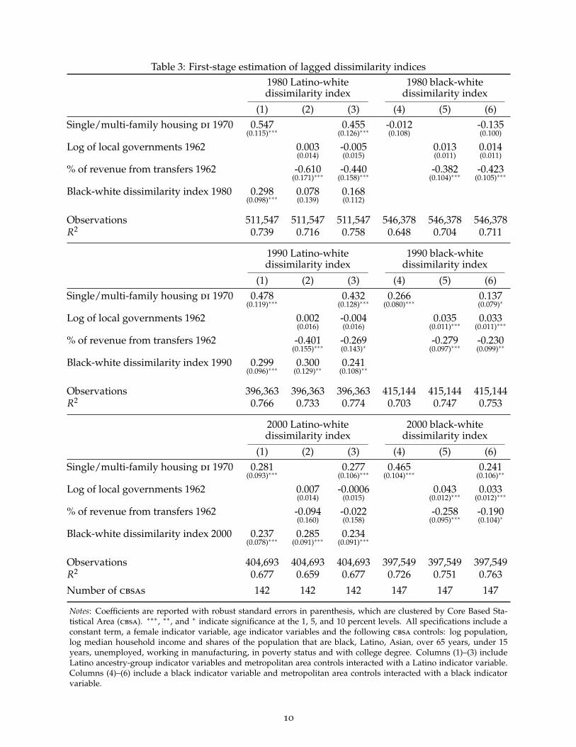
Table 3: First-stage estimation of lagged dissimilarity indices1980 Latino-white 1980 black-whitedissimilarity index dissimilarity index
(1) (2) (3) (4) (5) (6)Single/multi-family housing di 1970 0.547 0.455 -0.012 -0.135
(0.115)∗∗∗ (0.126)∗∗∗ (0.108) (0.100)
Log of local governments 1962 0.003 -0.005 0.013 0.014(0.014) (0.015) (0.011) (0.011)
% of revenue from transfers 1962 -0.610 -0.440 -0.382 -0.423(0.171)∗∗∗ (0.158)∗∗∗ (0.104)∗∗∗ (0.105)∗∗∗
Black-white dissimilarity index 1980 0.298 0.078 0.168(0.098)∗∗∗ (0.139) (0.112)
Observations 511,547 511,547 511,547 546,378 546,378 546,378R2 0.739 0.716 0.758 0.648 0.704 0.711
1990 Latino-white 1990 black-whitedissimilarity index dissimilarity index
(1) (2) (3) (4) (5) (6)Single/multi-family housing di 1970 0.478 0.432 0.266 0.137
(0.119)∗∗∗ (0.128)∗∗∗ (0.080)∗∗∗ (0.079)∗
Log of local governments 1962 0.002 -0.004 0.035 0.033(0.016) (0.016) (0.011)∗∗∗ (0.011)∗∗∗
% of revenue from transfers 1962 -0.401 -0.269 -0.279 -0.230(0.155)∗∗∗ (0.143)∗ (0.097)∗∗∗ (0.099)∗∗
Black-white dissimilarity index 1990 0.299 0.300 0.241(0.096)∗∗∗ (0.129)∗∗ (0.108)∗∗
Observations 396,363 396,363 396,363 415,144 415,144 415,144R2 0.766 0.733 0.774 0.703 0.747 0.753
2000 Latino-white 2000 black-whitedissimilarity index dissimilarity index
(1) (2) (3) (4) (5) (6)Single/multi-family housing di 1970 0.281 0.277 0.465 0.241
(0.093)∗∗∗ (0.106)∗∗∗ (0.104)∗∗∗ (0.106)∗∗
Log of local governments 1962 0.007 -0.0006 0.043 0.033(0.014) (0.015) (0.012)∗∗∗ (0.012)∗∗∗
% of revenue from transfers 1962 -0.094 -0.022 -0.258 -0.190(0.160) (0.158) (0.095)∗∗∗ (0.104)∗
Black-white dissimilarity index 2000 0.237 0.285 0.234(0.078)∗∗∗ (0.091)∗∗∗ (0.091)∗∗∗
Observations 404,693 404,693 404,693 397,549 397,549 397,549R2 0.677 0.659 0.677 0.726 0.751 0.763
Number of cbsas 142 142 142 147 147 147
Notes: Coefficients are reported with robust standard errors in parenthesis, which are clustered by Core Based Sta-tistical Area (cbsa). ∗∗∗, ∗∗, and ∗ indicate significance at the 1, 5, and 10 percent levels. All specifications include aconstant term, a female indicator variable, age indicator variables and the following cbsa controls: log population,log median household income and shares of the population that are black, Latino, Asian, over 65 years, under 15years, unemployed, working in manufacturing, in poverty status and with college degree. Columns (1)–(3) includeLatino ancestry-group indicator variables and metropolitan area controls interacted with a Latino indicator variable.Columns (4)–(6) include a black indicator variable and metropolitan area controls interacted with a black indicatorvariable.
10

contribute to predicting Latino-white dissimilarity in 1980 and 1990. The results in column (3)indicate that the coefficient on the housing type dissimilarity measure remains highly significantand does not experience a large change in its magnitude in the presence of the other instruments.We take this as evidence that our proposed instrument is strong. Further, the F-statistic reportedon the weak instruments identification test exceeds all thresholds proposed by Stock and Yogo(2005) for the maximal relative bias and maximal size in 1980 and 1990, though not in 2000.10 Asevidenced by the coefficients in columns (4) and (6), the housing type dissimilarity measure alsopredicts black-white dissimilarity in 1990 and 2000, though the strength of the prediction is not asstrong for black-white segregation as it is for Latino-white segregation, once other instruments areincluded.
We carry out several checks to validate our first stage results. First, to confirm that housingtype dissimilarity in 1970 was not the result of existing levels of Latino white segregation, wetest the relationship between the 1970 Latino-white dissimilarity index and our housing typedissimilarity index, controlling for log population of the metropolitan area in 1970, and do not finda statistically significant association.11 Second, higher levels of housing type dissimilarity in 1970
could have been more common in economically vulnerable and socially conservative metropolitanareas leading to more detrimental outcomes for minorities (Antecol and Cobb-Clark, 2008). Thebivariate relationships between metropolitan area characteristics in 1970 and our housing typedissimilarity measure actually show that more affluent metropolitan areas exhibited higher levelsof housing type dissimilarity.12 While we are unclear theoretically why this relationship exists, wecontrol for income, unemployment, college attainment, poverty rate and other metropolitan areacharacteristics in our first stage specifications. Third, we examine whether metropolitan areas withhigher levels of housing type dissimilarity experienced larger subsequent inflows of Latinos. Thiscould be a source of concern if Latinos disproportionately moved to these metropolitan areas basedon the availability of multi-family housing or another unobserved attribute correlated with thistype of housing (e.g. a booming construction sector). Specifically, we estimate regressions of ourhousing type dissimilarity index on the metropolitan area change in the share of Latinos between1970 and 1980, controlling for initial metropolitan area population, and do not find a significantassociation.13 Thus, historical housing configurations of some metropolitan areas contributed tothe segregation of Latinos from whites; however, they did not necessarily attract larger inflows of
10The F-statistic (or Kleinberger-Papp rk Wald statistic) exceeds 16 in 1980, 12 in 1990 and 4 in 2000. Only in 2000, itfalls slightly below the critical value for the 15% maximal iv size. This is in part due to the lack of significance of the twohistoric predictors of black-white segregation in column (3) of table 3 (bottom panel). Our estimates, shown in table 7,follow Wooldridge’s iv estimation adjustment (see Wooldridge, 2002) that uses as ‘instruments’ the predicted valueobtained for the Latino(black)-white dissimilarity index from the first-stage regression in table 3 and its interaction witha Latino(black) indicator variable.
11In complementary analogous estimations to our reported first-stage estimates, we control for other metropolitanarea variables in 1970 such as the log average household income and the proportion of the population that are Latino,black, unemployed, with college degree, in poverty status, and working in manufacturing, and again do not find astatistically significant association. Results available upon request.
12Metropolitan areas with higher housing type dissimilarity indices have a higher share of residents with a bachelor’sdegree, higher average household income, lower poverty rates and a lower share of Latino residents. Yet, they do nothave significant associations with the share of black residents or the proportion of workers in manufacturing.
13We obtain similar results when using the metropolitan area change in the share of Latinos between 1970 and 1990
as a dependent variable and when including a larger list of controls.
11

Table 4: Balancing tests of metropolitan area segregation on individual characteristics, 1990–2010Dependent variable: Latino-white lagged Black-white lagged
dissimilarity index dissimilarity index
(1) (2) (3) (4)
Female -0.012 -0.013 0.020 0.020(0.018) (0.022) (0.015) (0.016)
Age 26 0.022 0.022 0.021 0.020(0.026) (0.026) (0.019) (0.019)
Age 27 0.010 0.009 0.052 0.051(0.026) (0.027) (0.026)∗∗ (0.027)∗
Age 28 0.003 0.002 0.041 0.039(0.034) (0.035) (0.028) (0.029)
Age 29 -0.023 -0.025 0.045 0.043(0.047) (0.048) (0.034) (0.035)
Age 30 -0.041 -0.042 0.050 0.048(0.052) (0.054) (0.037) (0.038)
High school completed -0.056 -0.043(0.134) (0.096)
Associate degree -0.014 -0.195(0.116) (0.106)∗
College degree 0.071 0.309(0.157) (0.124)∗∗
F-test 0.920 0.12 1.12 2.09P-value 0.483 0.946 0.351 0.103
Observations 1,395,238 1,395,238 1,430,120 1,430,120R2 0.677 0.677 0.737 0.737
Notes: Coefficients are reported with robust standard errors in parenthesis, which are clustered by Core Based Sta-tistical Area (cbsa). ∗∗∗, ∗∗, and ∗ indicate significance at the 1, 5, and 10 percent levels. All specifications have aconstant term and census region-year indicator variables. Metropolitan area controls are listed in the notes of table 3.Sample in columns (1)–(2) is restricted to whites and Latinos. Sample in columns (3)–(4) is restricted to whites andblacks. See notes in table 1 for additional sample details. F-tests in columns (1) and (3) correspond to the joint effectof individual characteristics while in columns (2) and (4) correspond to the joint effect of the additional regressors onlevels of education.
Latinos compared to other metropolitan areas.Finally, we conduct balancing tests to examine the potential sorting of particular individuals
into metropolitan areas with different levels of segregation. The idea is to test whether observ-able individual characteristics (e.g. gender, age, and educational outcomes) are correlated withmeasures of segregation across metropolitan areas. If we do not find statistically significantassociations, then it is less likely that individuals sort into more or less segregated metropolitanareas based on unobserved characteristics (Bifulco, Fletcher, and Ross, 2011, Lou and Song, 2017).In table 4, we find no evidence that native-born white and Latino young adults have sorted onthose observable characteristics. We also allow for interactions between a Latino indicator variableand individual characteristics (results not shown) and do not find any significant association.Therefore, we find no indication of certain types of Latino or white young adults sorting basedon metropolitan area segregation.
12

4. Results
OLS results on the relation between segregation and individual outcomes
In table 5, we estimate ordinary least squares regressions of each individual outcome on metropoli-tan area levels of segregation, as well as individual and metropolitan area controls. We showresults with contemporaneous and lagged segregation levels (in which 1990 outcomes are linkedto 1980 segregation levels, etc.). We also show results for a regression with cbsa fixed effects withlagged segregation levels.14 In each pair of rows in the first panel, the first row reports the coeffi-cients on the metropolitan area Latino-white dissimilarity index and the second row the interactionbetween this index and a Latino indicator variable. For results in the top panel, the sample consistsonly of whites and Latinos, so the coefficient on the dissimilarity index can be interpreted as theassociation between Latino-white segregation and white outcomes, while the coefficient on theinteraction between the dissimilarity index and the Latino indicator variable shows any differencein the association between segregation and outcomes for Latinos as compared to whites. Standarderrors are clustered at the metropolitan area level.
Results reveal significant associations between metropolitan area segregation levels and everymeasured individual black and Latino outcome. Starting with the probability of having completedcollege for Latinos aged 25-30 in column (1), we find that the interaction coefficient is negativeand statistically significant, indicating that, in more segregated metropolitan areas, Latinos areless likely to complete college relative to their white counterparts. The results are similar whetherthe dissimilarity index is lagged or not, and, when metropolitan area fixed effects are included,the interaction coefficient increases in magnitude. A one standard deviation increase in theLatino-white dissimilarity index is related to a decline in the probability of finishing college of5.5 percentage points for Latinos relative to white graduation rates. The overall difference inthe means in college graduation rates for whites and Latinos, pooled across the 1990-2010 studyperiod, is 18.6 percentage points.
Looking at the incidence of being employed or in school again reveals that higher levels ofsegregation are consistently associated with a lower likelihood of being employed or in schoolfor Latino young adults relative to whites. A one standard deviation increase in the level ofsegregation is associated with a decrease in the likelihood of being either employed or in school forLatino 25-30 year olds relative to whites of 2.1 percentage points (the overall difference betweenwhites and Latinos in this age range is 5.1 percentage points).
As would be expected, the results with regard to professional occupations parallel the resultswith regard to college attainment. A one standard deviation increase in the Latino-white dissimi-larity index is related to a decline in the probability of professional employment of 3.7 percentagepoints for Latinos relative to white graduation rates (the overall difference in professional employ-ment rates between whites and Latinos is 11.7 percentage points).
As for income among 25-30 year olds, segregation is also associated with significantly largerLatino-white gaps. The results are consistent across all specifications and the magnitude is large.
14Results for cbsa fixed effects models are similar whether or not segregation is lagged.
13

Table 5: Estimation of the effect of segregation on individual outcomes, 1990–2010Dependent variable: College Not Professional Log annual
graduation idle occupation income
(1) (2) (3) (4)
Pooled ols,
Latino-white lagged dissimilarity index 0.032 0.037 0.011 0.127(0.043) (0.012)∗∗∗ (0.029) (0.081)
Latino-white lagged diss index × Latino -0.289 -0.141 -0.211 -0.657(0.041)∗∗∗ (0.019)∗∗∗ (0.028)∗∗∗ (0.086)∗∗∗
Pooled ols,
Latino-white dissimilarity index 0.031 0.036 0.009 0.146(0.045) (0.013)∗∗∗ (0.030) (0.085)∗
Latino-white diss index × Latino -0.330 -0.157 -0.228 -0.670(0.046)∗∗∗ (0.024)∗∗∗ (0.032)∗∗∗ (0.091)∗∗∗
cbsa,fixed-effects
Latino-white lagged dissimilarity index 0.080 0.019 0.046 0.146(0.041)∗ (0.015) (0.029) (0.081)∗
Latino-white lagged diss index × Latino -0.386 -0.149 -0.256 -0.653(0.051)∗∗∗ (0.021)∗∗∗ (0.035)∗∗∗ (0.073)∗∗∗
Observations 1,395,238 1,395,238 1,395,238 1,276,664Number of cbsas 187 187 187 187
Pooled ols,
Black-white lagged dissimilarity index 0.105 0.026 0.059 0.047(0.046)∗∗ (0.012)∗∗ (0.035)∗ (0.071)
Black-white lagged diss index × black -0.259 -0.151 -0.136 -0.404(0.048)∗∗∗ (0.022)∗∗∗ (0.034)∗∗∗ (0.091)∗∗∗
Pooled ols,
Black-white dissimilarity index 0.151 0.032 0.085 0.053(0.055)∗∗∗ (0.013)∗∗ (0.043)∗∗ (0.086)
Black-white diss index × black -0.280 -0.169 -0.129 -0.406(0.051)∗∗∗ (0.025)∗∗∗ (0.037)∗∗∗ (0.098)∗∗∗
cbsa,fixed-effects
Black-white lagged dissimilarity index -0.003 0.033 -0.005 0.122(0.069) (0.025) (0.039) (0.102)
Black-white lagged diss index × black -0.240 -0.132 -0.137 -0.436(0.055)∗∗∗ (0.021)∗∗∗ (0.032)∗∗∗ (0.078)∗∗∗
Observations 1,430,120 1,430,120 1,430,120 1,307,648Number of cbsas 184 184 184 184
Notes: Coefficients are reported with robust standard errors in parenthesis, which are clustered by Core Based Sta-tistical Area (cbsa). ∗∗∗, ∗∗, and ∗ indicate significance at the 1, 5, and 10 percent levels. In the top (bottom) panel,the sample is restricted to native-born whites and Latinos (blacks) between 25 and 30 years. All specifications havea constant term, a female indicator variable, age and census region-year indicator variables. The top panel includesLatino ancestry-group indicator variables, while the bottom panel includes a black indicator variable. Additional cbsa
controls include log population, log median household income and shares of population that are black, Latino, Asian,over 65 years, under 15 years, unemployed, working in manufacturing, in poverty status and with college degree.These cbsa controls are also interacted with a Latino or black indicator variable accordingly.
14
A one standard deviation increase in Latino-white segregation is associated with a 9.9 percentincrease in the gap between Latino incomes relative to whites. In the sample, annual income forwhites exceeds those for Latinos by 18.9 percent.
As shown in the second panel, the relationship between metropolitan area segregation andoutcomes among African American young adults is similar to that for Latinos. In more segregatedmetropolitan areas, black young adults are less likely to graduate from college, to be either inschool or employed, and to work in a professional occupation, and have lower incomes, relative towhites. The results are again robust to lagged dissimilarity and metropolitan area fixed effects.
In sum, higher levels of segregation are associated with worse educational and employmentoutcomes for both black and Latino young adults. The magnitudes of these negative associationsare larger for Latinos in every case except for the likelihood of being simultaneously out of workand out of school.15
We carried out alternative estimations that use the isolation index as the measure of metropoli-tan area segregation, estimated the same specifications for a younger sample of adults betweenthe ages of 20 and 24, and excluded recent (domestic) migrants from the sample. Results from allof these robustness tests, available upon request, are similar both in terms of significance andmagnitude of the effects. We also estimated regressions of black-white segregation on Latinooutcomes and of Latino-white segregation on black outcomes and found no significant associa-tions, suggesting that these results are not artifacts of unobserved metropolitan area characteristicsassociated with higher levels of residential segregation in general.16 In sum, our findings indicatethat Latino-white segregation has consistent negative associations with socio-economic outcomesfor Latino young adults relative to whites and black-white segregation has consistent negativeassociations with socio-economic outcomes for black young adults relative to whites.
The link between segregation and individual outcomes by ancestry
Examining the association between segregation and individual outcomes by ancestry in 2010
reveals considerable heterogeneity across groups.17 In table 6, we include interactions betweenthe dissimilarity index and seven ancestry groups (Cuban, Mexican, South American, CentralAmerican, Puerto Rican, Dominican and those who identified as ‘Other Hispanic’).18 Thus, thetotal effect of segregation in each of these groups is the sum of the general Latino interactioncoefficient and the ancestry group of interest. The association between segregation and outcomesis generally largest for Latinos who self-report having Puerto Rican or Dominican ancestry. For
15Note that the standard deviations of the Latino-white (0.144) and black-white (0.130) dissimilarity indices aresimilar. Thus, the magnitudes of the coefficients can be compared for both samples.
16Results available upon request.17The question on Latino ancestry identification varied in 2000 and this prevents us from establishing consistent
ancestry groups over time (Logan and Turner, 2013). We focus our analysis in 2010, when the Latino population in theUnited States is at its largest, most heterogeneous, and most geographically extensive.
18Sample sizes do not allow us to construct more narrow ancestry groups within Central and South America. Thetotal sample size for the Latino-white analyses in 2010 is 432,756 native born young adults, of which 359,903 (83.2%) arewhites. Of the Latinos in the sample, 47,256 (64.9%) identify their ancestry as Mexican, 11,590 (15.9%) as Puerto Rican,2,551 (3.5%) as Cuban, 2,902 (4.0%) as Central American, 1,482 (2.0%) as Dominican, 2,543 (3.5%) as South American,and 4,529 (6.2%) as ‘Other.’
15

Table 6: Estimation of the effect of segregation by Latino ancestry, 2010Dependent variable: College Not Professional Log annual
graduation idle occupation income
(1) (2) (3) (4)
Latino-white dissimilarity index 0.066 0.069 0.040 0.096(0.068) (0.017)∗∗∗ (0.045) (0.061)
Latino-white lagged di × other Latino -0.138 -0.063 -0.023 -0.303(0.086) (0.055) (0.072) (0.160)∗
Latino-white lagged di × Cuban -0.242 -0.059 -0.039 -0.050(0.159) (0.062) (0.095) (0.174)
Latino-white lagged di × Mexican -0.344 -0.110 -0.227 -0.516(0.068)∗∗∗ (0.034)∗∗∗ (0.049)∗∗∗ (0.093)∗∗∗
Latino-white lagged di × South American -0.511 -0.070 -0.413 -0.834(0.143)∗∗∗ (0.040)∗ (0.101)∗∗∗ (0.135)∗∗∗
Latino-white lagged di × Central American -0.545 -0.105 -0.333 -0.935(0.114)∗∗∗ (0.061)∗ (0.083)∗∗∗ (0.171)∗∗∗
Latino-white lagged di × Puerto Rican -0.614 -0.282 -0.451 -0.947(0.084)∗∗∗ (0.034)∗∗∗ (0.055)∗∗∗ (0.117)∗∗∗
Latino-white lagged di × Dominican Republic -0.685 -0.140 -0.584 -0.627(0.157)∗∗∗ (0.086) (0.121)∗∗∗ (0.212)∗∗∗
Latino ancestry-group indicators Yes Yes Yes Yes
Observations 432,756 432,756 432,756 395,742R2 0.093 0.033 0.048 0.064
Notes: Coefficients are reported with robust standard errors in parenthesis, which are clustered by Core Based Statisti-cal Area (cbsa). ∗∗∗, ∗∗, and ∗ indicate significance at the 1, 5, and 10 percent levels. Sample is restricted to native-bornwhites and Latinos between 25 and 30 years in 2010. Additional controls listed in notes of table 5 are included. The‘other Latino’ category includes those Latinos who self-report ‘Spaniard’ or ‘Other, not specified’ ancestry. di standsfor dissimilarity index.
instance, a one standard deviation increase in the dissimilarity index is associated for Puerto Ricanswith an 8.4 percentage-point decrease in the likelihood of attending college relative to whites, a 4.3percentage-point decrease in the likelihood of being employed or in school relative to whites, anda 13.7 percentage reduction in income relative to whites. This stronger association may reflect thelarger share of Puerto Ricans and Dominicans who are poor and identify or are perceived as black.
We see roughly similar associations for those who self-identified as having Central Americanancestry in terms of college graduation and income, but smaller associations between segregationand professional occupation as well as the likelihood of being simultaneously out of work andout of school. Segregation also has large negative associations with income and the likelihoodof being in a professional occupation for those who identify as having South American ancestry.The association between segregation and socio-economic outcomes is somewhat more modest forthose who identify as having Mexican ancestry, though the association with an increased likelihoodof being simultaneously out of school and out of work is large. Segregation has no negativeassociation with educational or labor market outcomes for those who identified Cuban ancestryand almost no negative association for those who identified their ethnicity as Hispanic, but theirancestry as ‘Other.’
16

Instrumental variable results
Table 7 presents the iv estimation of the effect of the Latino-white dissimilarity index on socio-economic outcomes in 1990, 2000, and 2010. The first two columns show results for 1990, withthe first column repeating the ols estimation for the 142 cbsas included in the sample and thesecond column showing iv estimates using all three instrumental variables discussed above forLatino-white segregation. The two subsequent rows within each panel show analogous results forblacks for a subset of 147 cbsas and iv estimates that use the same set of instrumental variablesfor black-white segregation. iv estimations use Wooldridge’s iv adjustment given that the sameinstruments are used to predict the coefficient on segregation and the interaction with the minorityindicator variable (see table note). Columns (3) and (4) show results for 2000, and columns (5) and(6) for 2010, all following the same pattern of ols estimations followed by iv estimations.
Instrumental variable estimates of the causal effect of segregation on racial or ethnic gaps incollege graduation show that segregation widens the gap in outcomes between whites and bothblacks and Latinos in all three decades. But in some years (2000 for blacks and 2010 for Latinos), thetotal effect of segregation (adding the coefficient on the dissimilarity index and the coefficient onthe interaction term) is zero or positive. Using the instrumental variable estimation, a one standarddeviation increase in metropolitan area segregation in 2010 had the effect of widening the gap incollege graduation rates between whites and Latinos by 8 percentage points, slightly more thanthe 5 percentage-point gap in the ols regression.
Regarding the likelihood of being either employed or in school, the iv results are significantand negative for Latinos in both 2000 and 2010 (as well as slightly larger than the ols results) butsignificant for blacks only in 2010. The 2 percentage-point gap between whites and Latinos causedby a one standard deviation increase in segregation is similar to the 1.6 percentage-point gap foundin the ols estimation.
For both blacks and Latinos, segregation widens the gap with whites in the likelihood ofprofessional occupation in all three decades. Further, when looking at point estimates the effectsof segregation on gaps in access to professional occupations were wider in 2000 and 2010 thanthey were in 1990. The magnitudes of the iv results are again larger than the ols estimates—a 6.9percentage-point gap caused by a one standard deviation increase in segregation compared to a3.5 percentage-point gap in the ols estimation.
Finally, with regard to income, the iv results are large, negative, and significant for both blacksand Latinos in all three decades. In fact, iv estimates indicate that a one standard deviation increasein the Latino-white dissimilarity index in 2010 almost doubles the income gap between Latinosand whites compared to ols estimates, from 8.1 to 15.3 percent. This causal effect of segregationaccounts for 56 percent of the total gap in earnings between Latinos and whites in 2010 (27.5percent). These earnings gaps have been remarkably persistent along the three decades.
Overall, the iv results present a relatively consistent story of negative effects of metropolitanarea segregation on socio-economic outcomes for both Latino and black young adults. Somewhatsurprisingly, the magnitudes of the effects of segregation are generally larger for Latinos than forAfrican-Americans. Also surprisingly, the negative effects of segregation for black young adults
17

Table 7: Instrumental variable estimation of the effect of segregation on individual outcomes1990 2000 2010
ols iv ols iv ols iv
(1) (2) (3) (4) (5) (6)
College graduation
Latino-white lagged diss index 0.072 0.433 0.046 0.535 0.014 0.827(0.054) (0.117)∗∗∗ (0.070) (0.197)∗∗∗ (0.076) (0.374)∗∗
Latino-white lagged di × Latino -0.280 -0.607 -0.422 -0.737 -0.421 -0.681(0.053)∗∗∗ (0.139)∗∗∗ (0.063)∗∗∗ (0.165)∗∗∗ (0.075)∗∗∗ (0.221)∗∗∗
Black-white lagged diss index 0.048 0.413 0.169 0.704 0.211 0.531(0.056) (0.162)∗∗ (0.054)∗∗∗ (0.156)∗∗∗ (0.071)∗∗∗ (0.128)∗∗∗
Black-white lagged di × black -0.149 -0.457 -0.343 -0.701 -0.372 -0.919(0.055)∗∗∗ (0.144)∗∗∗ (0.066)∗∗∗ (0.155)∗∗∗ (0.085)∗∗∗ (0.188)∗∗∗
Not idle,
Latino-white lagged diss index 0.028 0.067 0.021 0.060 0.023 0.019(0.014)∗∗ (0.027)∗∗ (0.016) (0.042) (0.020) (0.081)
Latino-white lagged di × Latino -0.144 -0.011 -0.193 -0.271 -0.138 -0.171(0.043)∗∗∗ (0.100) (0.030)∗∗∗ (0.058)∗∗∗ (0.033)∗∗∗ (0.059)∗∗∗
Black-white lagged diss index 0.069 0.164 0.040 0.109 0.050 0.088(0.018)∗∗∗ (0.043)∗∗∗ (0.015)∗∗ (0.030)∗∗∗ (0.018)∗∗∗ (0.039)∗∗
Black-white lagged di × black -0.114 -0.066 -0.144 -0.076 -0.114 -0.210(0.037)∗∗∗ (0.147) (0.028)∗∗∗ (0.072) (0.047)∗∗ (0.121)∗
Professional occupation
Latino-white lagged diss index -0.005 0.216 0.001 0.301 0.002 0.269(0.031) (0.070)∗∗∗ (0.039) (0.119)∗∗ (0.049) (0.176)
Latino-white lagged di × Latino -0.181 -0.361 -0.313 -0.671 -0.293 -0.583(0.046)∗∗∗ (0.101)∗∗∗ (0.040)∗∗∗ (0.118)∗∗∗ (0.048)∗∗∗ (0.130)∗∗∗
Black-white lagged diss index 0.036 0.222 0.095 0.400 0.101 0.237(0.032) (0.088)∗∗ (0.036)∗∗∗ (0.089)∗∗∗ (0.043)∗∗ (0.080)∗∗∗
Black-white lagged di × black -0.131 -0.277 -0.181 -0.458 -0.207 -0.475(0.040)∗∗∗ (0.105)∗∗∗ (0.044)∗∗∗ (0.127)∗∗∗ (0.058)∗∗∗ (0.115)∗∗∗
Log annual income
Latino-white lagged diss index 0.215 0.696 0.207 0.837 0.065 0.323(0.092)∗∗ (0.122)∗∗∗ (0.079)∗∗∗ (0.184)∗∗∗ (0.067) (0.322)
Latino-white lagged di × Latino -0.966 -1.707 -0.816 -1.567 -0.657 -1.205(0.145)∗∗∗ (0.309)∗∗∗ (0.107)∗∗∗ (0.234)∗∗∗ (0.088)∗∗∗ (0.209)∗∗∗
Black-white lagged diss index 0.030 0.363 0.201 0.867 0.197 0.497(0.098) (0.198)∗ (0.084)∗∗ (0.211)∗∗∗ (0.077)∗∗ (0.164)∗∗∗
Black-white lagged di × black -0.509 -0.884 -0.592 -0.680 -0.445 -0.975(0.144)∗∗∗ (0.467)∗ (0.132)∗∗∗ (0.344)∗∗ (0.116)∗∗∗ (0.256)∗∗∗
Notes: Coefficients are reported with robust standard errors in parenthesis, which are clustered by Core Based Statisti-cal Area (cbsa). ∗∗∗, ∗∗, and ∗ indicate significance at the 1, 5, and 10 percent levels. All specifications include a constantterm, a female indicator variable and age indicator variables. Controls included for cbsas and their interactionswith a Latino or black indicator variable are the ones listed in table B.12. The iv specifications for Latino-white andblack-white dissimilarity indices are columns (3) and (6) of table B.12, respectively. Regressions follow Wooldridge’siv estimation adjustment (see Wooldridge, 2002) that uses as ‘instruments’ the predicted value obtained for the Latino(black)-white dissimilarity index from the first-stage regression in table B.12 and its interaction with a Latino (black)indicator variable. di stands for dissimilarity index.
18

are largest in 2010, while the negative effects for Latino young adults are generally largest in 2000.The results also suggest some benefit to whites of segregated metropolitan areas for all four
measures of socio-economic outcomes in most specifications. These potential benefits for whitesare more significant for black-white segregation than Latino-white segregation, especially in 2010,and are particularly strong for college graduation and earnings. These findings are consistentwith Cutler and Glaeser (1997), who found that young white adults benefited from segregation in1990, at least with respect to college attainment. Segregation, by generating inequality in publicgoods and in social networks, is likely to both reinforce advantage and cumulate disadvantage bywidening inequality and facilitating resource hoarding (Durlauf, 2004, Graham, 2016).
Mechanisms
Table 8 examines mechanisms that can help explain how residential segregation translates intounequal individual outcomes. Using the Neighborhood Change Database developed by GeoLyticsand the Urban Institute, we construct weighted averages of neighborhood socio-economic charac-teristics. These weighted averages or exposure rates show the extent to which the average personof a specific race or ethnicity is exposed to a neighborhood characteristic. We construct measuresof exposure to poverty and exposure to neighbors with college degrees. We also use ipums data tocalculate the average growth in college graduate employment by three-digit industry in the nationas a whole between 1990 and 2010.19 We then calculate how exposed workers of different racesor ethnicities in each cbsa were to subsequent growing or declining industries. We subtract fromall our exposure measures the overall mean in the metropolitan area (calculated for all workersregardless of race) to avoid capturing differences in levels across metropolitan areas.
The exposure of white young adults to neighbors in poverty is associated with a decline inthe odds of being employed or in school. White exposure to neighbors with college degrees isassociated with an increase in college graduation and, relatedly, in the likelihood of working in aprofessional occupation.
The exposure of Latino young adults to individuals in poverty is associated with worse out-comes across the board, while exposure to neighbors with a bachelor degree is associated withan increased likelihood of college graduation. Latinos also benefit from being exposed to sectorsthat experienced notable skilled employment growth, in terms of college graduation, likelihood ofprofessional employment, and earnings.
Once we control for these exposures, the coefficient on Latino-white segregation interacted witha Latino indicator variable falls by between 48 and 67 percent, depending on the outcome. Largeunexplained effects remain for all outcomes.
The most consistent and largest iv results are the negative effects of segregation on black andLatino income in comparison to whites. To see how much of this effect could be explained bysegregation’s effects on educational attainment, we re-estimate our regressions of income, afteradding a set of binary variables indicating the educational level of the individual and their self-
19We construct time-consistent three-digit industry codes using the crosswalk provided in Autor and Dorn (2013).
19

Table 8: Potential mechanisms for the effects of Latino-white segregation, 2010Dependent variable: College Not Professional Log annual
graduation idle occupation income
(1) (2) (3) (4)
ols,
Latino-white lagged dissimilarity index 0.009 0.051 0.012 0.048(0.061) (0.016)∗∗∗ (0.039) (0.056)
Latino-white lagged diss index × Latino -0.364 -0.131 -0.253 -0.580(0.064)∗∗∗ (0.030)∗∗∗ (0.043)∗∗∗ (0.085)∗∗∗
ols including mechanisms
Latino-white lagged dissimilarity index -0.010 0.031 0.000 0.025(0.062) (0.018)∗ (0.040) (0.060)
Latino-white lagged diss index × Latino -0.119 -0.068 -0.094 -0.217(0.083) (0.041)∗ (0.063) (0.120)∗
White exposure to poverty × white 1.171 -0.459 0.783 -0.478(0.802) (0.233)∗∗ (0.563) (0.890)
White exposure to college × white 1.696 -0.041 1.064 -0.073(0.382)∗∗∗ (0.137) (0.270)∗∗∗ (0.419)
White exposure to industry growth × white -0.154 0.126 -0.012 -0.421(0.820) (0.180) (0.501) (0.866)
Latino exposure to poverty × Latino -0.559 -0.386 -0.428 -1.881(0.274)∗∗ (0.164)∗∗ (0.216)∗∗ (0.477)∗∗∗
Latino exposure to college × Latino 0.422 -0.156 0.188 -0.300(0.244)∗ (0.100) (0.171) (0.261)
Latino exposure to industry growth × Latino 0.199 0.032 0.177 0.386(0.088)∗∗ (0.064) (0.080)∗∗ (0.189)∗∗
Reduction in di coefficient for Latinos 67% 48% 63% 63%
Notes: Coefficients are reported with robust standard errors in parenthesis, which are clustered by Core Based Statisti-cal Area (cbsa). ∗∗∗, ∗∗, and ∗ indicate significance at the 1, 5, and 10 percent levels. Sample is restricted to native-bornwhites and Latinos between 25 and 30 years in 2010. Additional controls listed in notes of table 5 are included. Seemain text for an explanation on mechanisms.
reported English proficiency (whether they speak only English at home or speak it very well ascompared to not well or not at all). As shown in column (2) of table 9, the inclusion of educationand English proficiency explains just under 40 percent of the differences between blacks andwhites in annual income and half of the difference between Latinos and whites. When we shiftfrom examining log annual income to examining log hourly income, this still leaves significantdifferences between whites and Latinos in hourly income (though not between whites and blacks),even after controlling for education. In sum, a portion of the wider differences in income betweenwhites and minorities in more segregated metropolitan areas can be explained by differencesin educational attainment in those areas, and, for blacks, some of the differences can also beexplained by differences in participation or hours worked. For Latinos, we find that hourly incomeis significantly shaped by metropolitan area segregation, even after taking into account Englishproficiency, education and number of hours worked.
20

Table 9: Estimation of the effect of segregation on income, 1990–2010Dependent variable: Log annual income Log hourly income
(1) (2) (3) (4)
Pooled ols,
Latino-white lagged dissimilarity index 0.127 0.100 0.023 0.012(0.081) (0.083) (0.072) (0.073)
Latino-white lagged diss index × Latino -0.657 -0.368 -0.275 -0.138(0.086)∗∗∗ (0.081)∗∗∗ (0.067)∗∗∗ (0.067)∗∗
Pooled ols,
Latino-white dissimilarity index 0.146 0.129 0.049 0.042(0.085)∗ (0.089) (0.075) (0.077)
Latino-white diss index × Latino -0.670 -0.334 -0.293 -0.131(0.091)∗∗∗ (0.084)∗∗∗ (0.072)∗∗∗ (0.073)∗
cbsa,fixed-effects
Latino-white lagged dissimilarity index 0.146 0.083 0.072 0.036(0.081)∗ (0.073) (0.053) (0.049)
Latino-white lagged diss index × Latino -0.653 -0.309 -0.264 -0.093(0.073)∗∗∗ (0.054)∗∗∗ (0.044)∗∗∗ (0.034)∗∗∗
Education categories No Yes No YesEnglish proficiency No Yes No Yes
Observations 1,276,664 1,276,664 1,216,458 1,216,458Number of cbsas 187 187 187 187
Pooled ols,
Black-white lagged dissimilarity index 0.047 -0.0002 -0.008 -0.038(0.071) (0.064) (0.069) (0.063)
Black-white lagged diss index × black -0.404 -0.223 -0.012 0.081(0.091)∗∗∗ (0.074)∗∗∗ (0.063) (0.055)
Pooled ols,
Black-white dissimilarity index 0.053 -0.024 -0.005 -0.053(0.086) (0.074) (0.083) (0.075)
Black-white diss index × black -0.406 -0.204 0.051 0.153(0.098)∗∗∗ (0.080)∗∗ (0.070) (0.061)∗∗
cbsa,fixed-effects
Black-white lagged dissimilarity index 0.122 0.118 0.037 0.043(0.102) (0.102) (0.065) (0.067)
Black-white lagged diss index × black -0.436 -0.271 -0.082 0.001(0.078)∗∗∗ (0.060)∗∗∗ (0.048)∗ (0.038)
Education categories No Yes No YesEnglish proficiency No Yes No Yes
Observations 1,307,648 1,307,648 1,237,895 1,237,895Number of cbsas 184 184 184 184
Notes: Coefficients are reported with robust standard errors in parenthesis, which are clustered by Core Based Statis-tical Area (cbsa). ∗∗∗, ∗∗, and ∗ indicate significance at the 1, 5, and 10 percent levels. The same sample compositioncriteria and additional controls specified in notes of table 5 apply.
21

5. Discussion and conclusion
In summary, in our models with metropolitan-area fixed effects, segregation has only a weak ornon-existent association with the outcomes of whites, but it has a strong, negative association withthe educational and labor market outcomes of Latinos and blacks. As the level of segregationin a metropolitan area increases, the socio-economic outcomes of black and Latino young adultsliving in that metropolitan area deteriorate both absolutely and relative to whites. Among Latinos,segregation has a particularly negative association with the outcomes of young adults of PuertoRican and Dominican ancestry.
The instrumental variables results generally confirm the negative effects of segregation onblack and Latino young adults’ employment outcomes and indicate that, if anything, the ols
results understate the negative effects of segregation. These findings suggest that Latinos in moresegregated metropolitan areas have developed some means to mitigate the negative consequencesof segregation, yet, despite this attenuation, segregation’s effects remain large.
The instrumental variables results also suggest that whites in metropolitan areas with higherlevels of segregation are more likely to graduate from college. These positive effects of segregationon whites are most apparent in 2010, while the negative effects of segregation on Latino outcomesexhibit little variation between 2000 and 2010. Higher levels of black-white segregation alsoappear to lead to improved labor market outcomes for whites. On the one hand, whites maybenefit from segregation through the opportunity it affords to hoard resources, such as access tohigh-performing schools or neighborhoods with more highly educated peers. On the other hand,economic opportunities may happen to be greater and labor markets more robust in areas withgreater levels of segregation, but Latinos and blacks may be unable to access those benefits becauseof the physical and social barriers that residential segregation creates.
In short, our work makes clear that segregation heightens inequality between whites andLatinos. While the precise mechanisms are unclear, we provide suggestive evidence that part ofthe story is that residential segregation appears to lead to both differential exposure to growingindustries as well as differential exposure to peers and social networks, as proxied by neighbors’poverty and educational attainment.
References
Ananat, Elizabeth O. 2011. The wrong side(s) of the tracks: The causal effect of racial segregationon urban poverty and inequality. American Economic Journal: Applied Economics 3:34–66.
Antecol, Heather and Deborah A. Cobb-Clark. 2008. Racial and ethnic discrimination in localconsumer markets: Exploiting the army’s procedures for matching personnel to duty locations.Journal of Urban Economics 64(2):496–509.
Autor, David and David Dorn. 2013. The growth of low skill service jobs and the polarization ofthe us labor market. American Economic Review 103(5):1553–1597.
Bayer, Patrick, Hanming Fang, and Robert McMillan. 2014. Separate when equal? Racial inequalityand residential segregation. Journal of Urban Economics 82:32–48.
22

Bayer, Patrick, Stephen L. Ross, and Giorgio Topa. 2008. Place of work and place of residence:Informal hiring networks and labor market outcomes. Journal of Political Economy 116(6):1150–1196.
Bifulco, Robert, Jason M. Fletcher, and Stephen L. Ross. 2011. The effect of classmate characteristicson post-secondary outcomes: Evidence from the add health. American Economic Journal: EconomicPolicy 3(1):25–53.
Borjas, George. 1995. Ethnicity, neighborhoods, and human capital externalities. American EconomicReview 85(3):365–390.
Brueckner, Jan K. and Stuart S. Rosenthal. 2009. Gentrification and neighborhood housing cycles:will America’s future downtowns be rich? Review of Economics and Statistics 91(4):725–743.
Card, David and Jesse Rothstein. 2007. Racial segregation and the black-white test score gap.Journal of Public Economics 91(11–12):2158–2184.
Chetty, Raj, Nathaniel Hendren, Patrick Kline, and Emmanuel Saez. 2014. Where is the land ofopportunity? The geography of intergenerational mobility in the United States. Quarterly Journalof Economics 129(4):1553–1623.
Collins, Chiquita A. and David R. Williams. 1999. Segregation and mortality: The deadly effects ofracism? Sociological Forum 14(3):495–523.
Collins, William J. and Robert A. Margo. 2000. Residential segregation and socioeconomic out-comes: When did ghettos go bad? Economics Letters 69(2):239–243.
Cutler, David M. and Edward L. Glaeser. 1997. Are ghettos good or bad? Quarterly Journal ofEconomics 112(3):827–872.
Cutler, David M., Edward L. Glaeser, and Jacob L. Vigdor. 2008. When are ghettos bad? Lessonsfrom immigrant segregation in the United States. Journal of Urban Economics 63(3):759–774.
De la Roca, Jorge, Ingrid Gould Ellen, and Katherine M. O’Regan. 2014. Race and neighborhoodsin the 21
st century: What does segregation mean today? Regional Science and Urban Economics47:138–151.
Duncan, Brian and Stephen J. Trejo. 2011. Intermarriage and the intergenerational transmission ofethnic identity and human capital for Mexican Americans. Journal of Labor Economics 29(2):195–227.
Durlauf, Steven N. 2004. Neighborhood effects. In Vernon Henderson and Jacques-François Thisse(eds.) Handbook of Regional and Urban Economics, volume 4. Amsterdam: North-Holland, 2173–2242.
Edin, Per-Anders, Peter Fredriksson, and Olof Aslund. 2003. Ethnic enclaves and the economicsuccess of immigrants: Evidence from a natural experiment. Quarterly Journal of Economics118(1):329–357.
Ellen, Ingrid Gould. 2000. Is segregation bad for your health? The case of low birth weight.Brookings-Wharton Papers on Urban Affairs :203–238.
Epple, Dennis and Richard E. Romano. 2011. Peer effects in education: a survey of the theoryand evidence. In Jess Benhabib, Alberto Bisin, and Matthew O. Jackson (eds.) Handbook of SocialEconomics, volume 1. Amsterdam: North-Holland, 1053–1163.
23
Graham, Bryan S. 2016. Identifying and estimating neighborhood effects. Working Paper 22575,National Bureau of Economic Research.
Hoxby, Caroline M. 2000. Does competition among public schools benefit students and taxpayers?American Economic Review 90(5):1209–1238.
Kain, John F. 1968. Housing segregation, negro employment, and metropolitan decentralization.The Quarterly Journal of Economics 82(2):175–197.
Logan, John R. and Richard N. Turner. 2013. Hispanics in the United States: Not only Mexicans.Report, us2010 Project.
Lou, Tian and Tao Song. 2017. Ethnic segregation, education, and immigrants’ labor marketoutcomes. Processed, University of Connecticut.
Loury, Glenn C. 1977. A dynamic theory of racial income differences. In Phyllis A. Wallaceand Anette M. LaMond (eds.) Women, Minorities and Employment Discrimination. Lexington, ma:Lexington Books, 153–186.
Ludwig, Jens, Lisa Sanbonmatsu, Lisa Gennetian, Emma Adam, Greg J. Duncan, Lawrence F. Katz,Ronald C. Kessler, Jeffrey R. Kling, Stacy Tessler Lindau, Robert C. Whitaker, and Thomas W.McDade. 2011. Neighborhoods, obesity and diabetes—A randomized social experiment. NewEngland Journal of Medicine 365(16):1509–1519.
Pew Research Center. 2015. Modern immigration wave brings 59 million to u.s., driving popu-lation growth and change through 2065: Views of immigration’s impact on u.s. society mixed.Technical report, Pew Research Center, Washington, dc.
Portes, Alejandro and Julia Sensenbrenner. 1993. Embeddedness and immigration: Notes on thesocial determinants of economic action. American Journal of Sociology 98(6):1320–1350.
Rosenthal, Stuart S. and Stephen L. Ross. 2015. Change and persistence in the economic status ofneighborhoods and cities. In Gilles Duranton, Vernon Henderson, and William Strange (eds.)Handbook of Regional and Urban Economics, volume 5. Amsterdam: North-Holland, 1047–1120.
Ruggles, Steven, Katie Genadek, Ronald Goeken, Josiah Grover, and Matthew Sobek. 2015. Inte-grated Public Use Microdata Series: Version 6.0. Minneapolis, mn: University of Minnesota.
Sharkey, Patrick, Amy E. Schwartz, Ingrid Gould Ellen, and Johanna Lacoe. 2014. High stakesin the classroom, high stakes on the street: The effects of community violence on student’sstandardized test performance. Sociological Science 1:199–220.
Steil, Justin P., Jorge De la Roca, and Ingrid Gould Ellen. 2015. Desvinculado y desigual: Issegregation harmful to Latinos? The Annals of the American Academy of Political and Social Science660(1):57–76.
Stock, James H. and Motohiro Yogo. 2005. Testing for weak instruments in linear iv regression.In James H. Stock and Donald W. K. Andrews (eds.) Identification and Inference for EconometricModels: Essays in Honor of Thomas J. Rothenberg. Cambridge: Cambridge University Press, 109–120.
Tiebout, Charles M. 1956. A pure theory of local expenditures. Journal of Political Economy 64(5):416–424.
24

United States Bureau of the Census. 2010. Hispanic or Latino by specific origin. 2010 DecennialCensus Summary File 1. Retrieved from https://factfinder.census.gov/faces/tableservices/jsf/pages/productview.xhtml?pid=dec_10_sf1_pct11&prodType=table.
United States Bureau of the Census. 2013. Current Population Survey. Annual So-cial and Economic Supplement (asec) Supplement Survey, 2013. Retrieved fromhttps://www.census.gov/topics/population/hispanic-origin/data/tables.2013.html.
United States Department of Commerce, Bureau of the Census. 2001. Census of Governments,1962 and 1967. Ann Arbor, mi: Inter-university Consortium for Political and Social Research,https://doi.org/10.3886/icpsr00017.v1.
Weicher, John C. and Thomas G. Thibodeau. 1988. Filtering and housing markets: An empiricalanalysis. Journal of Urban Economics 23(1):21–40.
Wooldridge, Jeffrey M. 2002. Econometric Analysis of Cross Section and Panel Data. Cambridge, ma:The mit Press.
Appendix A. Assigning individuals in IPUMS to a Core Based Statistical Area (CBSA)
Barriers to using PUMAs
The smallest level of geography that can be identified in the Integrated Public Use MicrodataSample (ipums) is the Public Use Microdata Area (puma). pumas contain no fewer than 100,000
residents, are nested within state boundaries, and cover the entire United States. The CensusBureau oversees the delineation of pumas, which are redrawn for every decennial census. Becausepumas boundaries are not consistent across decennial censuses, they cannot be used to identifylocation patterns over time.
Barriers to using MSAs or CBSAs
Although ipums assigns observations to a ‘metropolitan area,’ the boundaries of any particularmetropolitan area change between censuses (generally becoming larger as the region grows).Therefore, we need to construct geographic units that generally correspond to metropolitan areasand are identical across the 1990, and 2000 Decennial Censuses, as well as the 2007–2011 AmericanCommunity Survey’s 5-year estimates.
Consistent PUMAs
We use publicly available ipums 5 percent unweighted samples. ipums-usa assigns every individ-ual observation to a puma and a ‘Consistent puma.’ Consistent pumas are the smallest geographicunits that do not change over time. Therefore, we can use them to link locations in the decennialcensuses and acs samples used in this study. The Consistent pumas contain no fewer than 400,000
residents, making them a significantly larger unit of geography than pumas.The Missouri Census Data Center provides a crosswalk from 2000 puma delineations to 2008
Cored Based Statistical Areas (cbsas). The crosswalk generates allocation factors for each puma,
25

indicating what percentage of the puma population falls within a particular cbsa. We assign anentire puma to a cbsa if more than 50% of the puma’s population lives within that cbsa. As a result,we build up a crosswalk that assigns each 2000 puma to a single cbsa or non-metropolitan area. Atotal of 1,694 pumas are linked to 353 cbsas.
As discussed, pumas cannot be used across years due to their boundaries being redrawn ineach census. However, given that all 2000 pumas also have a Consistent puma identifier, we cancreate a crosswalk that links Consistent pumas to cbsas. Using this crosswalk we can then assignindividual observations in the 1990 Census and the 2007–2011 acs data to a cbsa through theirConsistent puma identifier.
Assigning Consistent pumas to cbsas requires an additional level of assumptions. While someConsistent pumas are fully contained in large metropolitan areas, other Consistent pumas overlapseveral metropolitan areas or non-metropolitan areas. Using our crosswalk of 2000 pumas to 2008
cbsas and the population of each puma in 2000, we can calculate the share of the population foreach Consistent puma that lives in a particular cbsa. We then assign the whole population of theConsistent puma to the cbsa with the highest population share (as long as this share exceeds 50
percent of the Consistent puma’s population). We thus exclude those Consistent pumas whereno single cbsa contains more than 50 percent of the Consistent puma population. Of the 453
Consistent pumas that encompass some portion of a cbsa, we end up with 392 Consistent pumasin 242 cbsas. Most of the cbsas that we lose have small populations.
The assignment of individuals to cbsas through Consistent puma identifiers results in geo-graphic areas that are comparable over time. However, the cbsa boundaries we obtain do notcorrespond exactly to census cbsa boundaries. For example, a Consistent puma may have 51% ofits population within a cbsa but 49% within a non-metropolitan area; our method would essen-tially redraw the cbsa boundary to include this non-metropolitan area. Likewise, if a Consistentpuma overlaps two cbsas, then our method would entirely allocate this Consistent puma to a singlecbsa as long as the share of its population in this cbsa exceeds 50%. Furthermore, some parts ofcbsas are ignored when Consistent pumas partially overlap multiple geographic areas and do nothave half or more of their population within any one cbsa.
One potential concern is that the use of Consistent pumas may result in improper assignment ofobservations to cbsas due to the large size of Consistent pumas. We can examine the extent of thisproblem for the year 2000. As already mentioned, the crosswalk provided by the Missouri CensusData Center links 2000 ipums data to cbsas. We estimate our specifications for 2000 using bothpuma to cbsa assignment and the coarser Consistent puma to cbsa assignment. The two methodsgive generally consistent results.
26

Appendix B. Online appendix
Table B.10: First-stage estimation of lagged dissimilarity indices, 1980Dependent variable: 1980 Latino-white 1980 black-white
dissimilarity index dissimilarity index
(1) (2) (3) (4) (5) (6)Single/multi-family housing di 1970 0.547 0.455 -0.012 -0.135
(0.115)∗∗∗ (0.126)∗∗∗ (0.108) (0.100)
Log of local governments 1962 0.003 -0.005 0.013 0.014(0.014) (0.015) (0.011) (0.011)
% of revenue from transfers 1962 -0.610 -0.440 -0.382 -0.423(0.171)∗∗∗ (0.158)∗∗∗ (0.104)∗∗∗ (0.105)∗∗∗
Black-white di 1980 0.298 0.078 0.168(0.098)∗∗∗ (0.139) (0.112)
Log population -0.018 0.015 -0.005 0.069 0.050 0.054(0.015) (0.018) (0.019) (0.009)∗∗∗ (0.013)∗∗∗ (0.013)∗∗∗
% black population -0.004 0.398 0.135 0.151 0.277 0.344(0.198) (0.212)∗ (0.198) (0.101) (0.094)∗∗∗ (0.094)∗∗∗
% Latino population 0.928 0.827 0.854 -0.122 -0.069 -0.079(0.135)∗∗∗ (0.161)∗∗∗ (0.148)∗∗∗ (0.094) (0.113) (0.107)
% Asian population -0.445 -0.255 -0.399 -0.321 -0.141 -0.096(0.238)∗ (0.276) (0.243) (0.129)∗∗ (0.138) (0.144)
% population over 65 1.887 2.372 1.741 0.486 0.120 0.281(0.572)∗∗∗ (0.527)∗∗∗ (0.538)∗∗∗ (0.450) (0.406) (0.396)
% population under 15 0.851 1.257 0.817 -0.141 -0.328 -0.229(0.579) (0.529)∗∗ (0.523) (0.534) (0.462) (0.469)
% unemployed 1.085 1.329 0.826 0.853 0.622 0.777(0.904) (0.890) (0.904) (0.734) (0.747) (0.723)
% working in manufacturing 0.620 0.665 0.777 0.425 0.461 0.416(0.255)∗∗ (0.305)∗∗ (0.261)∗∗∗ (0.242)∗ (0.245)∗ (0.248)∗
% in poverty status -0.422 -0.547 -0.190 0.089 0.181 0.070(0.488) (0.554) (0.511) (0.443) (0.449) (0.448)
% with bachelor’s degree 0.478 0.789 0.491 -0.388 -0.379 -0.291(0.361) (0.393)∗∗ (0.339) (0.237) (0.226)∗ (0.225)
Log median household income 0.034 0.069 0.036 0.011 -0.013 -0.003(0.046) (0.049) (0.043) (0.027) (0.023) (0.027)
Observations 511,547 511,547 511,547 546,378 546,378 546,378Number of cbsas 142 142 142 147 147 147R2 0.739 0.716 0.758 0.648 0.704 0.711
Notes: Coefficients are reported with robust standard errors in parenthesis, which are clustered by Core Based Sta-tistical Area (cbsa). ∗∗∗, ∗∗, and ∗ indicate significance at the 1, 5, and 10 percent levels. All specifications include aconstant term, a female indicator variable and age indicator variables. Columns (1)–(3) include Latino ancestry-groupindicator variables and cbsa controls interacted with a Latino indicator variable. Columns (4)–(6) include a blackindicator variable and cbsa controls interacted with a black indicator variable. di stands for dissimilarity index.
27

Table B.11: First-stage estimation of lagged dissimilarity indices, 1990Dependent variable: 1990 Latino-white 1990 black-white
dissimilarity index dissimilarity index
(1) (2) (3) (4) (5) (6)Single/multi-family housing di 1970 0.478 0.432 0.266 0.137
(0.119)∗∗∗ (0.128)∗∗∗ (0.080)∗∗∗ (0.079)∗
Log of local governments 1962 0.002 -0.004 0.035 0.033(0.016) (0.016) (0.011)∗∗∗ (0.011)∗∗∗
% of revenue from transfers 1962 -0.401 -0.269 -0.279 -0.230(0.155)∗∗∗ (0.143)∗ (0.097)∗∗∗ (0.099)∗∗
Black-white di 1990 0.299 0.300 0.241(0.096)∗∗∗ (0.129)∗∗ (0.108)∗∗
Log population -0.017 0.001 -0.010 0.064 0.038 0.033(0.012) (0.016) (0.014) (0.009)∗∗∗ (0.013)∗∗∗ (0.013)∗∗
% black population -0.016 0.168 0.059 0.158 0.382 0.344(0.130) (0.128) (0.120) (0.096)∗ (0.094)∗∗∗ (0.094)∗∗∗
% Latino population 0.799 0.666 0.745 -0.098 0.002 0.032(0.110)∗∗∗ (0.116)∗∗∗ (0.113)∗∗∗ (0.088) (0.108) (0.108)
% Asian population -0.382 -0.220 -0.354 -0.299 0.043 0.004(0.155)∗∗ (0.182) (0.168)∗∗ (0.115)∗∗∗ (0.128) (0.135)
% population over 65 1.977 2.288 1.824 1.239 1.279 1.127(0.628)∗∗∗ (0.610)∗∗∗ (0.620)∗∗∗ (0.548)∗∗ (0.498)∗∗ (0.494)∗∗
% population under 15 0.951 1.382 0.915 -0.312 -0.067 -0.175(0.713) (0.762)∗ (0.678) (0.849) (0.724) (0.719)
% unemployed 0.504 1.527 0.481 -0.266 -0.421 -0.780(1.151) (1.024) (1.096) (1.071) (0.858) (0.864)
% working in manufacturing 0.678 0.540 0.758 1.024 0.680 0.731(0.213)∗∗∗ (0.268)∗∗ (0.253)∗∗∗ (0.231)∗∗∗ (0.256)∗∗∗ (0.248)∗∗∗
% in poverty status 0.126 0.055 0.256 0.187 0.083 0.144(0.400) (0.421) (0.442) (0.471) (0.447) (0.427)
% with bachelor’s degree 0.669 1.005 0.686 -0.164 -0.090 -0.184(0.262)∗∗ (0.305)∗∗∗ (0.260)∗∗∗ (0.186) (0.179) (0.174)
Log median household income 0.084 0.115 0.087 -0.047 -0.047 -0.055(0.057) (0.059)∗∗ (0.052)∗ (0.030) (0.028)∗ (0.029)∗
Observations 396,363 396,363 396,363 415,144 415,144 415,144Number of cbsas 142 142 142 147 147 147R2 0.766 0.733 0.774 0.703 0.747 0.753
Notes: Coefficients are reported with robust standard errors in parenthesis, which are clustered by Core Based Sta-tistical Area (cbsa). ∗∗∗, ∗∗, and ∗ indicate significance at the 1, 5, and 10 percent levels. All specifications include aconstant term, a female indicator variable and age indicator variables. Columns (1)–(3) include Latino ancestry-groupindicator variables and cbsa controls interacted with a Latino indicator variable. Columns (4)–(6) include a blackindicator variable and cbsa controls interacted with a black indicator variable. di stands for dissimilarity index.
28
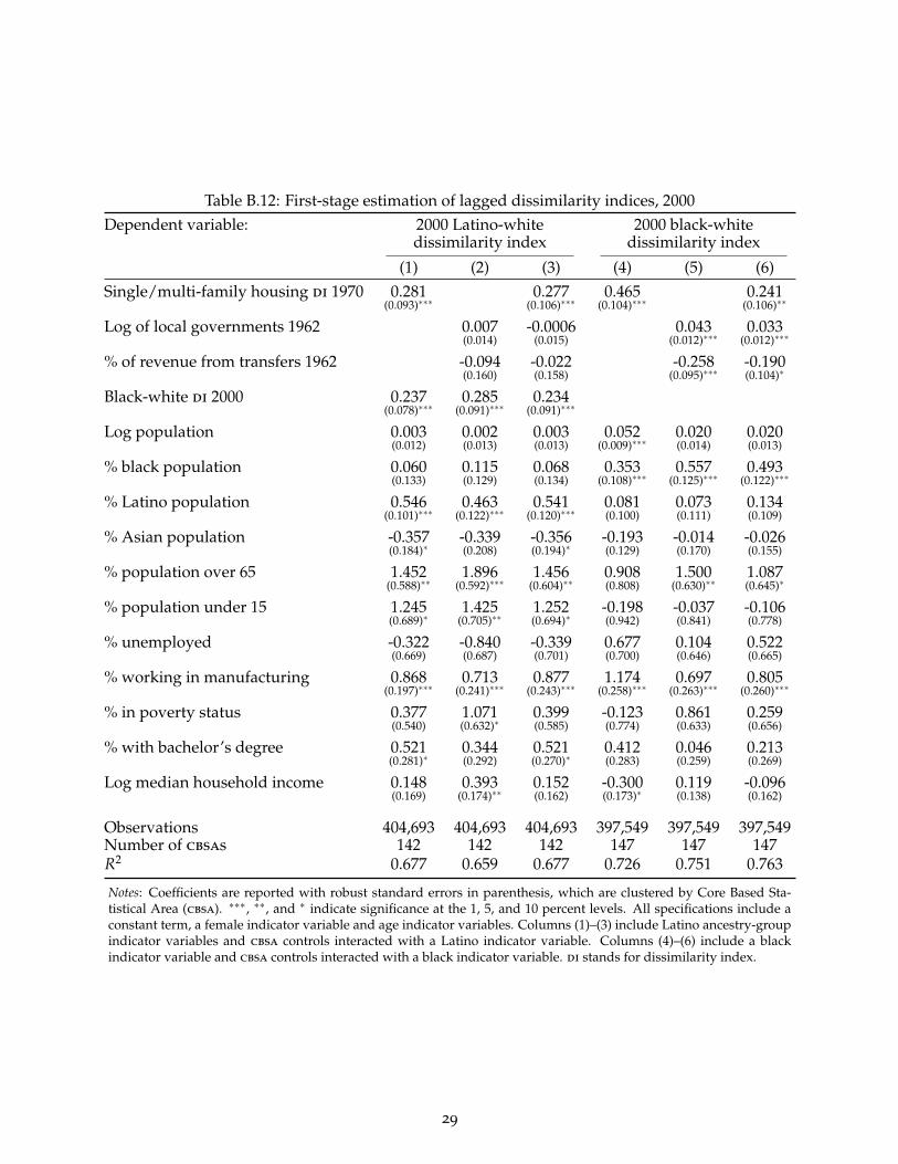
Table B.12: First-stage estimation of lagged dissimilarity indices, 2000Dependent variable: 2000 Latino-white 2000 black-white
dissimilarity index dissimilarity index
(1) (2) (3) (4) (5) (6)Single/multi-family housing di 1970 0.281 0.277 0.465 0.241
(0.093)∗∗∗ (0.106)∗∗∗ (0.104)∗∗∗ (0.106)∗∗
Log of local governments 1962 0.007 -0.0006 0.043 0.033(0.014) (0.015) (0.012)∗∗∗ (0.012)∗∗∗
% of revenue from transfers 1962 -0.094 -0.022 -0.258 -0.190(0.160) (0.158) (0.095)∗∗∗ (0.104)∗
Black-white di 2000 0.237 0.285 0.234(0.078)∗∗∗ (0.091)∗∗∗ (0.091)∗∗∗
Log population 0.003 0.002 0.003 0.052 0.020 0.020(0.012) (0.013) (0.013) (0.009)∗∗∗ (0.014) (0.013)
% black population 0.060 0.115 0.068 0.353 0.557 0.493(0.133) (0.129) (0.134) (0.108)∗∗∗ (0.125)∗∗∗ (0.122)∗∗∗
% Latino population 0.546 0.463 0.541 0.081 0.073 0.134(0.101)∗∗∗ (0.122)∗∗∗ (0.120)∗∗∗ (0.100) (0.111) (0.109)
% Asian population -0.357 -0.339 -0.356 -0.193 -0.014 -0.026(0.184)∗ (0.208) (0.194)∗ (0.129) (0.170) (0.155)
% population over 65 1.452 1.896 1.456 0.908 1.500 1.087(0.588)∗∗ (0.592)∗∗∗ (0.604)∗∗ (0.808) (0.630)∗∗ (0.645)∗
% population under 15 1.245 1.425 1.252 -0.198 -0.037 -0.106(0.689)∗ (0.705)∗∗ (0.694)∗ (0.942) (0.841) (0.778)
% unemployed -0.322 -0.840 -0.339 0.677 0.104 0.522(0.669) (0.687) (0.701) (0.700) (0.646) (0.665)
% working in manufacturing 0.868 0.713 0.877 1.174 0.697 0.805(0.197)∗∗∗ (0.241)∗∗∗ (0.243)∗∗∗ (0.258)∗∗∗ (0.263)∗∗∗ (0.260)∗∗∗
% in poverty status 0.377 1.071 0.399 -0.123 0.861 0.259(0.540) (0.632)∗ (0.585) (0.774) (0.633) (0.656)
% with bachelor’s degree 0.521 0.344 0.521 0.412 0.046 0.213(0.281)∗ (0.292) (0.270)∗ (0.283) (0.259) (0.269)
Log median household income 0.148 0.393 0.152 -0.300 0.119 -0.096(0.169) (0.174)∗∗ (0.162) (0.173)∗ (0.138) (0.162)
Observations 404,693 404,693 404,693 397,549 397,549 397,549Number of cbsas 142 142 142 147 147 147R2 0.677 0.659 0.677 0.726 0.751 0.763
Notes: Coefficients are reported with robust standard errors in parenthesis, which are clustered by Core Based Sta-tistical Area (cbsa). ∗∗∗, ∗∗, and ∗ indicate significance at the 1, 5, and 10 percent levels. All specifications include aconstant term, a female indicator variable and age indicator variables. Columns (1)–(3) include Latino ancestry-groupindicator variables and cbsa controls interacted with a Latino indicator variable. Columns (4)–(6) include a blackindicator variable and cbsa controls interacted with a black indicator variable. di stands for dissimilarity index.
29