Does Oil Corrupt? Evidence from a Natural Experiment … · 1 Does Oil Corrupt? Evidence from a...

1

Does Oil Corrupt?

Evidence from a Natural Experiment in West Africa∗

Pedro C. Vicente1

Forthcoming at the Journal of Development Economics

Abstract: This paper explores the oil discovery announcements in Sao Tome and Principe (1997-1999) to assess the role of natural resources in determining corruption. For this purpose, we use a natural experiment framework which contrasts Sao Tome and Principe to Cape Verde, a control West African country sharing the same colonial past and important recent economic and political shocks. Our measurement is based on tailored household surveys we conducted in both island countries. The unique survey instrument was retrospective and used personal histories to elicit memories from the respondents. We analyze changes in perceived corruption across a wide range of public services and allocations. We find clearest increases on vote buying, education (namely in the allocation of scholarships) and customs, ranging from 31 to 40% of the subjective scale. We interpret these findings as symptoms of increased competition for core state resources. JEL Codes: D73, O13, O55, P16. Keywords: Corruption, Political Economy, Natural Resources, Curse, Oil, West Africa, Sao Tome and Principe, Cape Verde.

∗ I wish to thank primarily Cátia Batista, Marianne Bertrand, Casey Mulligan, Roger Myerson, the editor Anne Case, and two anonymous referees for detailed comments. I am also grateful for suggestions to Abigail Barr, Paul Collier, Marcel Fafchamps, Nicola Gennaioli, Steven Levitt, Kenneth Rasinski, Allen Sanderson, Gerhard Seibert, Susan Stokes, Robert Townsend and Christopher Udry. I thank participants in seminars at SSE, Cornell, Oxford, ISEG-UTL, Yale, Navarra, Aarhus, UQAM and Chicago, and conference presentations at CSAE, GPRG, EEA, Econometric Society World Congress and CESifo for useful comments. I am grateful for institutional support to Lúcio Pinto at Instituto Superior Politécnico of Sao Tome and Principe and Deolinda Reis at the Instituto Nacional de Estatística of Cape Verde, to my co-interviewers in the surveys conducted, C. Castro, A. Coelho, E. Lima, A. Pinto, H. Santos, D. Solé, E. Solé, D. Vicente (Sao Tome and Principe) and C. Andrade, E. Fernandes, A. Gonçalves, V. Lenine, H. Mendes, R. Moniz, L. Pina, A. Semedo, N. Varela (Cape Verde), and to the 1907 respondents who answered our questions with generosity. I gratefully acknowledge financial support from Fundação para a Ciência e a Tecnologia (BD1215/2000), Henry Morgenthau Jr. Memorial Fund, Department of Economics at the University of Chicago, and ESRC-funded Global Poverty Research Group. All remaining errors are my responsibility alone. 1 Email: [email protected]. Affiliations: Trinity College Dublin, Department of Economics, Arts Building, Dublin 2, Ireland; CSAE – Centre for the Study of African Economies, University of Oxford; BREAD - Bureau for Research and Economic Analysis of Development.

2

“It's because of oil that they want to take over power”. - Fradique de Menezes, President of the Democratic Republic of São Tomé and Príncipe, after July 2003 coup attempt “The international community should investigate the activities of

successive governments in São Tomé”. - Fernando Pereira “Cobo”, July 2003 coup attempt leader

1 Introduction

Economists have long studied natural-resource curses. The precursor was the Dutch Disease, i.e.

the statement that resource booms, through the appreciation of the real exchange rate, reduce the

competitiveness of non-resource sectors, and correspondingly TFP growth rates (Corden and

Neary, 1982; van Wijnbergen, 1984; Krugman, 1987). More recent theories of resource booms

have highlighted the importance of rent seeking (Tornell and Lane, 1999; Baland and Francois,

2000; Torvik, 2002) and political corruption under fragile institutions (Robinson et al, 2006)2.

In the face of such theoretical detail, the literature’s empirical counterpart has only given us two

clear findings, both in the context of cross-country data: resource-rich countries do tend to grow

more slowly (Sachs and Warner, 1995), and especially when they have weak institutional

frameworks (Mehlum et al, 2006). Hence, not much is clear about the empirical mechanisms of

resource curses. The main objective of this paper is to contribute along this dimension, by

exploring the empirical effects of an oil discovery announcement on corruption3, using a natural

experiment setting with micro data measurement4.

In this paper we analyze the significant oil discovery announced in the period 1997-1999 in Sao

Tome and Principe, a low-income West African island-country neighbored by well known

resource-cursed countries (Equatorial Guinea, Gabon and Nigeria). We hypothesize (as do

Robinson et al, 2006) that these announcements increased the value to politicians of being in

power, leading both to more resources being spent on improving the likelihood of being elected

2 Other recent work relates natural resources with conflict – Bannon and Collier (2003), Collier and Hoeffler (2004) – and with dictatorships – Jensen and Wantchekon (2004). 3 As in Bardhan (1997), we take corruption as ‘abuse of public office for private gain’. See Becker and Stigler (1974), Rose-Ackerman (1978), Cadot (1987), Klitgaard (1988), Myerson (1993) for early approaches to the economics of corruption. 4 Some cross-country work linking natural resources to higher corruption was performed by Leite and Weidman (1999) and Ades and Di Tella (1999). Coupled with Mauro (1995), who shows a negative effect of corruption on growth, this line of work conveys a full curse-through-corruption narrative.

3

and to resource misallocation in the rest of the economy. The implication is an increase in

corruption, primarily in politics (of which vote buying is the clearest example), but also,

potentially, in many public services and allocations.

Our identification strategy is based on the comparison of Sao Tome and Principe with a control

West African island-country, Cape Verde. Both countries were under Portuguese colonial rule

until 1975 (a period close on five centuries). Moreover, these nations had remarkably similar

political and economic shocks after independence: in both, their first regime was socialist, ending

in 1991 when the first free elections were run (in both countries); in parallel with

democratization, aid levels increased and foreign-induced economic reforms were implemented.

We argue that the comparison between Sao Tome and Principe and Cape Verde will allow us to

control for these important macro-level post-independence shocks. In the face of the Sao Tomean

oil discovery, this comparison will then serve as a suitable natural experiment5.

Measurement in this paper is founded on tailored representative household surveys on perceived

corruption conducted by the author in both Sao Tome and Principe (841 interviews) and Cape

Verde (1066 interviews) after the oil discovery period. Perceived corruption questions were asked

regarding a wide range of public services and allocations: courts of law, customs, education

(about primary and secondary schools and concerning the allocation of scholarships),

infrastructure construction decisions, health care, license emission, police, the allocation of jobs

in the public sector, subsidies and state procurement (for suppliers of the state), and electoral

politics (vote buying). Importantly, the unique survey instrument used personal historical

markings gathered at the beginning of the interview as elicitors of memory for retrospective

measures of corruption (while only asking corruption questions of subjects reporting experience

with the corresponding public services or allocations). In addition, several measures of pessimism

over time (‘good old times’) were collected to control for any differing bias across treatment and

control groups.

Our main estimation approach is based on a standard difference-in-difference estimator

(identifying the difference between Sao Tome and Principe and Cape Verde, before–after the oil

discovery period, through comparing perceptions about the periods 1991 to 1997 and 2000 to the

5 In the disperse corruption literature other naturally occurring micro frameworks have recently been explored to derive causes of corruption: Duggan and Levitt (2000), Fisman (2001), Fisman and Miguel (2007).

4

‘present’), while controlling for differing characteristics of the country samples (from a wide

range of survey demographic measurements) and differing time pessimism. However, we also

attempt to improve on the raw perceptions of representative households as the basis of our

estimates of changes in corruption. With this objective, we apply an additional margin of

comparison in a triple-difference econometric approach, by which more- and less-informed

(about public services and allocations) respondents are contrasted. Our identifying assumption is

that both informed and uninformed subject groups may be subject to perception biases (like

unfounded public opinion), which we want to remove from our estimates. We use different

measures of information in trying to capture alternative dimensions of experience among

respondents.

We found clear increases on perceived corruption in a number of public services and allocations

after the Sao Tomean oil discovery, most solidly on vote buying, education, and customs. While

vote buying and corruption in customs are already prominent in the difference-in-difference

approach, corruption in scholarship allocations appears very clearly only in our triple-difference

estimation. Other services and allocations also yield significant increases in corruption, though

with lower magnitude and robustness: primarily in courts and the allocation of

subsidies/procurement and state jobs, but also on health care and police (the latter only significant

in one of the triple-difference variants). However, we do not observe statistical significance with

respect to infrastructures and licenses.

We interpret these results as indicative of increased competitiveness for state resources, namely

those that are accessible through the political channel. The effect on vote buying points squarely

in this direction, but the effect on higher education can also be interpreted in this vein, given the

prominent social status of scholarships for studying abroad. The effect on corruption in customs

may be a symptom of increased private consumption by the Sao Tomean elite (potentially funded

with oil-related moneys). Less clear effects on health and police may be due to relative scarcity in

those sectors as a consequence of inefficient allocation of state resources, in line with the

theoretical literature. Generally, we take this pattern of corruption change to indicate support of

political and institutional resource curses.

The paper proceeds as follows. First we contextualize our natural experiment, while depicting

basic features of Sao Tome and Principe and Cape Verde. We then present our main theoretical

hypothesis and corresponding identification strategy. In the following section, we describe the

5

data collection process, with both sampling and instrument design. We then devote our attention

to the empirical results, with basic descriptive statistics and alternative estimation strategies. We

finally conclude.

2 Historical Background

The empirical focus of this paper is on two island-countries in West Africa, Sao Tome and

Principe (STP) and Cape Verde (CV). STP is the second smallest country in sub-Saharan Africa

with 155 thousand inhabitants in 2006 and is composed of two main islands; CV has 519

thousand residents (2006) and is constituted by nine inhabited islands6. Both countries were

Portuguese colonies for close on 500 years, having both gained independence in the context of the

latest wave of African decolonization in 1975.

Since the focus of this paper is on institutional outcomes, we shall draw attention to the

remarkably similar political history of STP and CV. Both countries had autocratic socialist

regimes until 1989, at which point democratization was initiated, culminating in the first multi-

party elections to be run in both countries in 1991. In these elections (and contrary to the majority

of African countries), the incumbent was ousted in both parliamentary and presidential contests.

It is worth mentioning that electoral cycles and changes of parties in power were also very close

in both countries7.

In terms of economic shocks, we highlight that, contemporaneously to the democratization

period, a series of IMF and World Bank sponsored economic reforms (macroeconomic

stabilization/price liberalization, privatization plans - namely with respect to land ownership)

were implemented in both countries. Related to the fact that both countries have been classified as

‘low-income’ (World Bank) during the whole period of analysis in this paper, aid per capita

patterns (which in STP accounted for an average 53% of the state revenues in the period 1992-

20048) stayed on strikingly similar levels for most of the democratic period. OECD data on total

grant disbursements points to averages of 0.30 and 0.27 USD per capita/year for STP and CV

6 Population figures are provided by the World Development Indicators, World Bank, 2008. 7 Elections in STP: 1991 (Presidential PR/Parliamentary PL); 1994 (PL), 1996 (PR), 1998 (PL), 2001 (PR), 2002 (PL), 2006 (PR/PL). Elections in CV: 1991 (PR and PL); 1995 (PL), 1996 (PR), 2001 (PR/PL), 2006 (PR/PL). 8 See IMF Country Reports 98/93, 02/31, 04/107 and 06/329.

6

respectively over the period 1991-20059. A further point on the economy relates to the higher

importance of agriculture in STP, namely in the context of the long-running tradition of cocoa

production and exporting (80% of all exports10) in that country: from the late 80s, international

cocoa prices have been stable (17% standard deviation in the period 1989-2005)11, and we are

therefore confident that no differential shocks occurred in STP and CV for this reason in the

period 1991 to present.

It is also worth commenting on the strong cultural links these two countries share: important

waves of emigration from CV to fertile STP took place in the twentieth century, in the context of

the Portuguese colonial economic strategy. Carreira (1982) reports that almost 35 thousand Cape

Verdeans left for STP in the period 1950-1970. However most Cape Verdeans are accounted as

having returned immediately after the collapse of Portuguese rule in 1975: indeed, only 1.9% of

the population in the 2001 Sao Tomean census had Cape Verdean nationality. Moreover, this

segment of the population tends to be older, more rural, and poorer than either the average Sao

Tomean or Cape Verdean12. The recent size of the Cape Verdean community in STP and its

demographic profile reassure us that any shock affecting STP is not likely to have a relevant

impact in CV.

The events that constitute our focus in this paper occurred late in the nineties. During the period

1997-1999 there was a series of announcements regarding the existence of offshore oil in STP13.

It all began with a contract for soundings and exploration with a small US company in 1997,

accompanied by the first estimates of oil reserves off the coast of STP. But only late in 1998,

when ExxonMobil was given preferential rights for exploration, did the oil discovery earn

widespread credibility. In 1999 a joint exploration deal was agreed with Nigeria (due to unclear

maritime territory demarcation). The first round of auctions for offshore oil blocks occurred in

2003: highest bids amounted to 237% of STP’s GDP. Note that various accusations of corruption

in these early oil-related contracts signed by the STP government were being made from the

9 Seibert (2006), who presents a comprehensive study on the history of STP, underlines that the democracy path was the result of a recognition that the support of western countries and institutions would mean better offers of aid. 10 CIA World Factbook. 11 IMF Primary Commodity Prices, 2008, deflated using US Department of Labor CPI. 12 This pattern stands out in our representative surveys of Sao Tomean and Cape Verdean households. 13 Refer to Vicente (2006) for a detailed chronology of oil-related events in STP.

7

discovery years - see Frynas et al (2003) for a detailed description14. We argue these facts created

the exogenous variation in our natural experiment15. Crucially, oil has never been found in CV to

date and is said to be very unlikely to exist or to have viable exploration in its territory16.

In this setting, can we find external evidence in favor of our main hypothesis, i.e. that corruption

may have increased in STP relative to CV after the oil discovery announcements? Indeed, it

seems to be corroborated by the only international cross-country index of corruption perceptions

that is available for STP: the World Bank Institute’s Governance Indicators (Kaufmann et al,

2008), available from 1998. In Chart 1 we see a clear divergence path across the two countries,

with corruption clearly increasing in STP after 1999.

Finally, since we are going to focus our attention in the specific pattern of change of corruption

across public services and allocations, we display in Chart 2 the cross-sector pattern of public

investment in STP over the period 1992-2004 (IMF). Note that total public investment increased

on average by 6.2% per year during this period. We can observe a striking fact: an overwhelming

increase of investment in ‘public administration’ occurred after 1999, with health, education and

infrastructures facing a relatively stable sequence of investment over the whole period. We can

also observe that resources devoted to agriculture are clearly decreasing over time, given the

14 For a more recent account of facts, see: ‘Sao Tome – where the Champagne Swills in before the Oil Gushes Out’, Financial Times, March 25th/26th 2006; ‘Ressources Naturelles, Mercenaires et Pressions Géopolitiques: Fiévre Pétrolière à Sao-Tome-et-Principe’, Le Monde diplomatique, October, 2006; ‘No Oil yet, but African Isle Finds Slippery Dealings’, New York Times, July 2nd, 2007. 15 In Shadish et al (2002), a natural experiment is defined as stemming from a ‘naturally occurring event, one that cannot be manipulated’. 16 See Prime-Minister Neves side-declarations to Radio Comercial of CV in June 2003.

-0.6

-0.4

-0.2

0

0.2

0.4

0.6

0.8

1

1998 1999 2000 2001 2002 2003 2004 2005

Cor

rupt

ion

Scal

e (-

2.5

to 2

.5)

Chart 1: Corruption Perceptions Index (World Bank), STP vs. CV

STP

CV

STP OIL DISCOVERY

Source: World Bank - WBI, Kaufmann et al (2008).

8

foreign-induced privatization reforms already mentioned. These findings set the stage for our in-

depth analysis of corruption before and after the Sao Tomean oil discovery.

3 Experimental Design

3.1 Hypothesis

The main hypothesis under analysis in this paper is whether there is a political resource curse.

The recent paper by Robinson et al (2006) builds a theoretical model in which they find that

‘resource booms, by raising the value of being in power and by providing politicians with more

resources which they can use to influence the outcome of elections, increase resource

misallocation in the rest of the economy’. However this outcome critically depends on the initial

quality of institutions (political accountability): indeed, these authors argue that countries without

such institutions may suffer from a political resource curse. Note that the resource-misallocation

implication had already been the main contribution of Tornell and Lane (1999), Baland and

Francois (2000), and Torvik (2002), who emphasized (with slightly different variations) an

increase in inefficient activities like rent-seeking. However these authors did not assume an

explicitly electoral motive for these effects to emerge.

STP provides a stellar setting for the analysis of this proposition. We postulate that the oil-

discovery announcements of the period 1997-1999 increased the value of being in power in STP

(when oil-related revenues are available). If STP has in place low levels of political

0

10

20

30

40

50

60

1992 1993 1994 1995 1996 1997 1998 1999 2000 2001 2002 2003 2004

% A

nnua

l Pub

lic

Inve

stm

ent

Chart 2: Public Investment by Sector in STP

Public Administration

Agriculture and Fisheries

Public Infrastructures

Education

Health

Source: IMF Country Reports, 98/93, 02/31, 04/107, and 06/329.

9

accountability, despite the fact that it has been a working democracy since 1991, we shall observe

changes in corruption that are in accord with Robinson et al. First of all on the conduct of

elections (namely on electoral corruption), given the focus on gaining/maintaining political

power. Yet, other sectors and allocations where the state has an important influence could also

witness changes in corruption. These additional movements unrelated to electoral behavior could

originate not only in the same political power-seeking mechanism (for instance, if these

allocations facilitate future political power), but also in the simple public-resource misallocation

that is deduced by Robinson et al. In the latter case, a shift of resources towards the higher-valued

‘political’ allocations would increase relative scarcity of resources in non-‘political’ sectors (like

the ones relating to standard public services). Higher competition in these non-‘political’

allocations could then arise, leading to increased corruption in those sectors.

In the empirical analysis that follows, we aim at measuring the impact of the oil discovery

announcements on the level of corruption in different public services and allocations of STP. Our

prior premise is that by investigating the pattern of cross-sector corruption, we may throw some

light on the empirical validity of the political resource curse hypothesis (as posed above). We

designed our empirical measurement in such a way as to allow information-gathering about a

quasi-complete range of sectors/allocations where the state has a relevant direct role, and where

corruption could be responding to the exogenous resource boom. Different sectors and allocations

can sensibly be taken to embody in different ways the two mechanisms referred - power-seeking,

clearly associated with vote buying; and relative scarcity, plausibly linked (for example) to the

health sector. That is the assumed variation we intend to explore later in the paper to reconcile our

findings with theory. We are, however, alert to the fact that our cross-sector general

interpretations may be made difficult by idiosyncratic (and sometimes unknown to us) conditions

in specific public services and allocations of STP and CV.

3.2 Identification

Empirically we will focus on measuring proxies of corruption across public services and

allocations. Our identification strategy makes central use of the natural experiment setting that

was created between STP and CV with the exogenous oil discovery of the late nineties. Our

estimation approach is built around a standard difference-in-difference (STP vs. CV, before vs.

after) design.

10

We argue in this paper that a Cape Verdean sample may provide a competent control group for

our perceptions of interest for two main reasons. First, STP and CV are similar countries, with

comparable institutional frameworks and demographics (as we will be able to show in a precise

manner with our representative samples of both countries). They share the same cultural roots,

actively nurtured by Portuguese colonization up until 1975. Second, they share strikingly similar

recent political shocks, with socialist first-regimes and democratization/corresponding foreign-

induced economic reform starting at the end of the eighties. Note that the trend induced by this

shock, arguably the most important in the post-colonial period, could have been confounded in

the pure before-after difference in STP, had we not contrasted this first margin with the

corresponding Cape Verdean one in a difference-in-difference strategy.

Our time difference is enabled by a careful retrospective measurement within our surveys. This

measurement was based on using personal history markings over time (elicited at the start of the

survey questionnaire) to locate in time the questions about corruption perceptions in the different

services and allocations. The exact same technique, with the same memory elicitors, was used in

both countries.

The possibility that respondents, despite the implementation of the described measurement

technique, are still subject to a retrospective bias like the ‘good old times’ predisposition (by

which respondents may tend to spuriously report worsening conditions over time), is not, in our

view, a major threat to our identification strategy. This is for two reasons. First, if this bias is

comparable across STP and CV, it should disappear when we control for CV perceptions

(collected under the exact same conditions). Second, we gathered different measures of

pessimism over time, including a placebo time difference: we gathered corruption perceptions

about two different periods in the past when nothing major happened in either country. We are

therefore able to control for pessimism in our regressions.

We are then ready to present our main difference-in-difference regression specification:

iltlllitilt TfteTdtcYbXaC ε++++++= * , (1)

11

where C is a corruption outcome, i, l, t are identifiers for individuals, locations, and time (pre-oil

with value 0 and post-oil with value 117), T is a binary variable with value 1 for ‘treated’ locations

(STP, with value 1, CV with value 0), X is a vector of demographic and attitudinal controls, Y is a

geographical fixed effect. Our coefficient of interest in this specification is the interaction

coefficient f.

Note that in the presence of observable differences between the STP and CV samples, controlling

for X and Y may improve on the precision of the coefficient of interest (see Kling et al, 2007, for a

recent example).

In the final part of the paper, we will attempt to identify our target parameter in a subtler way by

trying to control for spurious changes in perceptions (e.g. through speculative public opinion

induced by widespread media). By assuming that both informed and uninformed groups may be

subject to a bias of this kind, we propose to add a further difference to our identification strategy

through the comparison of more- and less-informed respondents. In addition, by building on an

additional difference in our empirical strategy, we are able to further validate our assertion that

the results of the double-difference comparison are not driven by an unexplained difference in

trends between STP and CV.

The triple-difference regression specification is represented in the following equation:

iltililiillliilt GTktGjTGhtgGTfteTdtcYbXaC ε++++++++++= ***** , (2)

where G is a relevant internal-to-a-country margin of information about corruption. Our main

coefficient of interest in this specification is the full interaction coefficient, k.

This triple-difference rationale is based on finding suitable proxies of informed respondents. We

use two different variables, which we hope can be regarded as complementary.

We contrast urban with rural respondents as a way of putting the emphasis on the eminently top-

down nature of our theoretical hypothesis (any reaction to the oil discovery is born in the political

sphere); we are implicitly assuming that the political sphere is urban, since capital cities (in these

17 Note that, as Bertrand et al (2004) point out, the fact that we collapse time series variation into before/after periods, minimizes standard error biases from serial correlation.

12

small countries) are where most politicians (and definitely the most important ones) are based.

This proxy may have the disadvantage of being less precise in terms of identifying experience

with public services and allocations per se.

The other proxy we use employs a number of survey questions aimed at constructing an index of

usage and provision of public services for each respondent (a connectivity index). The advantage

and disadvantage of this proxy are the reverse of the ones described for the urban/rural

comparison: connectedness with services is obviously good, in that it provides better information

about those services; however, it may be blinder to centrality and therefore to our relevant top-

down theoretical hypothesis.

Note that this information margin has an obvious limitation: for services and allocations for

which both informed and uninformed respondents have knowledgeable perceptions, corruption

effects should be deservedly similar across urban and rural respondents. In this sense, when using

the information difference, we may be estimating a lower bound for our effects of interest.

In all specifications in this paper we allow for correlation in the error term by clustering at the

level of the enumeration area.

4 Data Collection: Tailored Household Surveys on Corruption

Data analyzed in this paper come from household surveys conducted by a team recruited and

trained by the author, and which included the author, in STP (Apr./May 2004), and in CV (Dec.

2005/Feb. 2006)18. In STP the survey was submitted to 841 households in 30 of the 149

enumeration (census) areas (20%) of the country (on average approximately 28 interviews per

area were conducted). In CV the survey was submitted to 1066 households (though only 997

respondents completed the full length of the interview) in 30 of the 561 enumeration (census)

areas (6%) of the country (on average 36 interviews per area).

4.1 Sampling

18 For details of fieldwork activities in both surveys, including maps of enumeration areas, visit http://users.ox.ac.uk/~econ0192/fieldwork.htm.

13

Our country survey samples were subject to a standard two stage sampling design, which first

selected clusters (enumeration areas), and then households, guaranteeing that the probability that

a given household was chosen was a priori the same across all households. We aimed at

nationally representative samples of households, since most of our questions concerned the

experience of households (as the relevant unit) about public services and allocations.

In specific terms, our sampled enumeration areas were chosen randomly, weighting by the

number of households19. Selected households were distributed as evenly as possible across the

census area, as we sought the nth house (depending on the number of households at each

area) in each enumeration area. In each selected household we invited one individual (a

household ‘representative’) to answer the questionnaire. This subject was required to be 30 years

or older, and had to fulfill a residence criterion for the country of surveying in our periods of

interest – before and after the oil discovery announcements, 1991-1997 and 2000-‘present’. These

criteria ensured that subjects could be knowledgeable about the public sector of their country in

the past.

Two sources of imperfection in the sampling of households should be mentioned: non-

respondents20, and differences in the number of targeted respondents across enumeration areas21.

The first problem was mitigated through data collection: when targeted respondents refused to

answer, interviewers would take note of their gender, approximate age, schooling and income,

and these data allowed us to draw a profile of non-respondents. All econometric work presented

in this paper uses weights22 to account for the two identified departures from perfect household

random sampling. This is for consistency with the sampling approach and does not change our

results in any relevant way.

4.2 Survey Instrument Design: Recall, ‘Good Old Times’, and Corruption Perceptions

19 The data that enabled this exercise (i.e. the distribution of households across the territory, from the 2000/2001 censuses in both countries) were provided by the National Statistics Offices of both countries. Note that in CV an additional cluster was used: the choice of 4 out of the 9 islands, which was weighted by population. 20 In this survey this problem was not significant by common standards in the survey literature: identified non-respondents amounted to 8.5% (STP) and 16% (CV) of the identified sample. 21 Namely, an oversample of the two enumeration areas of the island of Principe (STP) took place. 22 Standard techniques were followed - see Deaton (1997).

14

The survey instrument we used in both STP and CV was tailored to allow accurate measurement

of corruption perceptions in a wide range of public services and allocations for both periods of

interest in this paper (before and after the oil discoveries, 1991 to 1997 and 2000 to ‘present’)23.

We therefore devoted special attention to the difficulties of measuring perceptions about the past.

Namely we implemented specific techniques to improve recall and to measure a ‘good old times’

type of retrospective bias.

To improve on recall, the questionnaire asked questions about specific public services and

allocations of the households/individuals who had experience with those particular

services/allocations (this was assessed by asking directly or indirectly about that experience), and

elicited respondents’ memories by making use of their household’s historical markings24.

Since the questionnaire began with non-sensitive demographic questions (e.g. children’s ages)25,

interviewers had a demographic profile of the respondent available from the very beginning of the

interview. This information was useful in identifying legitimate respondents to specific questions

(e.g. a sufficient condition to answer the questions on the health care services was to have had at

least one child) and in eliciting memories/probing, as the interviewers always referred to our

periods of interest in a personal manner. (For example, for the subject whose first child had been

born in 1994, in the health care services question the interviewer referred to the period before-oil

announcement, 1991-97, as the period when the respondent's first child was born). Whenever

experience with a particular service/issue was not assessed (and corresponding memory elicitors

were not gathered) with the initial demographic part of the interview, specific questions regarding

that experience were posed just before asking the corresponding corruption-perception questions

(with corresponding answers used as memory elicitors). All experience assessors in the

questionnaire are used in building our connectivity index, which is included in our triple

difference identification strategy26.

Concerning the possibility of a ‘good old times’ bias, a placebo difference was elicited for

questions on corruption in health care, as we anticipated it to be the most frequently

23 The final version of the survey instruments is available in the original Portuguese (the official language of both STP and CV) and as an English translation from the author’s webpage. 24 This technique is well known in the survey design literature (see for instance Rasinski, Rips and Tourangeau, 2000). 25 Questions regarding more sensitive demography were presented at the end of the questionnaire (e.g. political preferences, income). 26 See Vicente (2006) for the specific components and corresponding weights used in this index.

15

answered question on standard perceived corruption (the pre-oil period 1991-1997 was

divided into 1991-1994 and 1994-1997, and both periods were used as independent periods of

interest); and two ‘agree/disagree’ (on a 1-7 subjective scale) questions were included concerning

general time-pessimism (phrased as ‘good times were those when you were young’ and ‘the

future of your country will be better than the present’). This information enables us to generate

measures of pessimism over time, which will become useful control variables later on in this

study.

Corruption-perception questions27 encompassed a wide range of public services and allocations.

These questions concerned the courts of law, customs, the allocation of scholarships for higher

education abroad, schools (primary and secondary), health care, infrastructures (public

construction decisions), license emission services, police, the allocation of jobs in the state, the

allocation of state subsidies and procurement (supplying contracts), and electoral politics (i.e.

vote buying). The corruption questions were always asked in a general, non-personal manner,

making sure respondents felt secure/relaxed in answering. In this paper we focus on questions on

general undue influence (the only ones asked across time), as opposed to questions about crude

bribery28. As a representative example, the precise phrasing of the relevant question for

corruption in the allocation of scholarships was (translation): ‘In the Sao Tomean/Cape Verdean

reality, when allocating scholarships for higher education abroad, what has been the need to know

someone important?’ (Answers were on a ‘Necessary/Not necessary’ scale, with 7 different

points). Note, however, that not all questions were formulated using this explicit/negative tone.

Some questions were asked using a naïve tone, i.e. asking whether the services were

functioning according to ‘the rules’ (specifying those rules for the corresponding service).

This mix worked as a balancer of tone in the interviews, as we wanted to minimize the

pessimistic tone embedded in the pure act of asking about corruption.

It should be noted that all questions on subjective assessments (including the corruption

questions) were given a 1 to 7 scale. Importantly, all these questions were approached in a two-

stage iterative process: when asking a question, the interviewer referred first to the three basic

27 See Bertrand and Mullainathan (2001) for a review of the main difficulties of using/designing subjective data. 28 See Vicente (2006) for a comparison of these different measures of corruption for STP and CV: it is shown that influence is more prevalent than crude bribery in both countries (generally across all services and allocations) and that its pattern is more similar (than that of bribery) when contrasting our STP and CV samples.

16

scale options 1-3, 4, and 5-7 (e.g. ‘important’ 1-3, ‘neither important nor unimportant’ 4, and

‘unimportant’ 5-7); when the subject chose one of these options, the interviewer, in the first and

last cases, asked about the different possibilities within the class already identified by the

respondent29. Note that all numbers had a precise language counterpart (using qualifiers, e.g.

‘extremely’, ‘very’, ‘somewhat’), which was the only way used by the interviewers to refer to

scales while surveying.

5 Empirical Results

5.1 Descriptive Statistics

We begin by contrasting our samples for STP and CV in terms of basic characteristics. In Tables

1 and 2 we display averages per country with corresponding standard errors.

Concerning central demographics we find more female respondents were recruited in CV than in

STP – this is due to the open sampling method we used, which asked for a household

‘representative’ and therefore allowed different household patterns to emerge. Cape Verdean

respondents are also older by two years on average. More Cape Verdeans live in STP (5.7%) than

the reverse (just 1.1%), which confirms the mid 20th century migration pattern already mentioned.

The main ethnic group in our STP sample is Forro (56.4%), while most of our CV respondents

are originally from Santiago Island (54%). A clear majority of the respondents considers itself to

be Catholic (75% in STP and 88% in CV). Both household size and number of children are

reported to be slightly higher (by one individual on average) in our Sao Tomean sample; very

similar patterns of children’s schooling are found in both countries. More STP subjects consider

themselves to be in an unmarried union.

We also collected information on patterns of education, occupation, and income. In terms of

education, schooling seems to be slightly higher in our STP sample (on average, with some

secondary level studies – represented by point 4 in our scale). However, enumerators classified

CV respondents as more fluent in the language of the questionnaire, Portuguese. In occupation, a

clearly higher number of Sao Tomeans is linked to agriculture (50.2% vs. 20.4% in CV) and

industry (9.3% vs. 1.6% in CV). However, for other sectors of activity differences are small:

29 These procedures were implemented in an attempt to increase the likelihood that the scale was perceived as equidistant (linearly) by respondents.

17

construction, commerce, transports, public administration, education and health care. CV

respondents seem to compensate in terms of household work (41.7% vs. 30.2% in STP) and

unemployment. Consistently with macro income data, household expenditure is reported to be

higher in CV than in STP. (Using middle points in the expenditure classes used, we find

expenditure per capita to be 0.98 USD in STP and 1.6 USD in CV). More land is held in STP by

respondents to our survey (consistent with a more important agricultural sector). However,

houses, cars and cattle are more frequently owned by Cape Verdeans.

Past base voting is divided between three political ‘families’ in STP, formed over time:

MLSTP/Pinto da Costa (president during the period 1975-1991) with 28.6%, ADI/Miguel

Trovoada (1991-2001) with 14.1%, and MDFM/Fradique de Menezes (2001 to present) with

35.6%. In CV politics are more clearly bipartisan, with PAICV, the independence party, getting

23.5% of respondents in our sample, and MPD holding 28.6% of base self-reported voters.

Political interest seems to be slightly higher in STP.

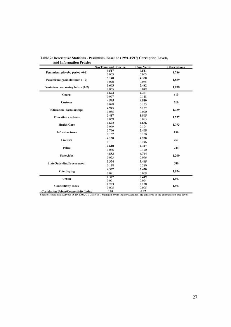
A note is also due on our pessimism measures (displayed in the top panel of Table 2). As per the

placebo difference described above, we do not find significant differences between the STP and

CV samples. We do, however, find some differences in our general question measures, which

seem to indicate that Sao Tomean respondents are more pessimistic.

In the middle panel of Table 2 we present our baseline corruption averages for both countries.

Corruption in 1991-1997 was considered to be higher in STP in terms of vote buying, undue

influence in construction contracts, courts and education (schools), but lower for favoritism in the

allocation of scholarships. For all other services/allocations, differences are not statistically

significant. Note that corruption is reported to be the highest for scholarship allocations in both

countries, followed by state jobs and health care in STP, and customs and state jobs in CV;

though questions on education (schools), infrastructures and state subsidies/procurement are not

directly comparable in absolute terms (given the different tone used in the questionnaire).

Finally, in the bottom panel of Table 2 we display descriptive statistics for our proxies of

information, to be used in our triple-difference identification strategy. The STP sample is slightly

less urban30 but more ‘connected’ than the CV sample. Note that these two dimensions yield a

30 Our classification of urban locations was: for STP - all enumeration areas in Água Grande (the district composed of the capital city and its suburbs) and the census area of Trindade-Cruzeiro (corresponding to

18

positive but low correlation (0.08 in STP and 0.07 in CV), which is consistent with a

complementary role in our exercise.

From this comparative analysis we can conclude that our STP and CV samples, although yielding

similar general demographic patterns, still present some different characteristics. In the

regressions we show in this paper, we control for the wide range of individual demographic and

pessimism observables described in this section, including all the ones where significant

differences between the two countries were found.

5.2 Difference-in-Difference Estimates: Sao Tome and Principe vs. Cape Verde

In Tables 3 and 4 we show the econometric results of our main specification (1), from which we

can identify the difference in corruption perceptions between the two country samples, before-

after the oil discovery announcements. This is our main proposed margin of identification of the

effect of the oil discovery on perceptions of corruption in public services and allocations of STP.

We begin by displaying OLS regressions where we only control for district fixed effects (Table

3)31. We can observe clear positive and significant interaction coefficients for all outcomes of

interest apart from corruption in construction projects (where statistical significance is not

achieved – note however that this question had very restrictive criteria for being asked and

therefore yields a low number of observations). Note that for most sectors/allocations, statistical

significance is realized at the 1% level.

Within these positive estimates, we can, however, distinguish a clear pattern of heterogeneity.

Largest effects (above or equal to 10% of the subjective scale) are for customs and vote buying.

Next, still in the top five, are corruption in state job allocations and distribution of subsidies/state

procurement, both with 9%, and in the courts of law, with 8%. Then, by decreasing order of

interaction coefficient estimates, we have corruption in education (schools), state licenses,

education (scholarships), health care and police.

the center of the second city of the country, itself in the outskirts of the capital district); for CV: all enumeration areas in the capital Praia (with the exception of suburb-village São Martinho Grande) and in Mindelo, the two major cities of the country. 31 We have undertaken separate robustness checks, using unweighted observations, interviewer fixed effects, and Ordered Probit, to account for corruption-scale non-linearities. None of these altered our estimates in any relevant way – all these additional exercises are available upon request from the author.

19

We can also observe (ceteris paribus) that Cape Verdean respondents generally reported an

increase in corruption in the period ‘2000 to present’ (with the exception of the allocations of

subsidies/procurement); and that for the baseline period, for customs and subsidies/procurement

only, Sao Tomeans reported lower corruption than Cape Verdeans.

Note that these results already indicate major effects in high level, political allocations (vote

buying). The effect on customs yields a less clear interpretation: it may be associated with the

clear increase in imports of non-food consumption goods over our period of interest32, and

indicative that there could already be sectors of STP society with increased wealth (spent outside

the country) after the oil discovery (consistent with persistent rumors of corrupt oil deals, as

mentioned above).

Note also that services and allocations where there is closer proximity to core state resources,

state jobs, subsidies and state procurement, and courts of law (where top politicians have been

handling accusations of corruption in recent years) see higher increases in perceived corruption

than, for instance, health care and police - where the link to top public administration is clearly

less direct.

We now add individual controls to our regressions (Table 4). As mentioned above, these

comprise all demographic33 and pessimism dimensions discussed in Section 5.1. Specifically we

use the same variables for all regressions, both for modeling consistency and to retain strict

comparability. Importantly, these variables include our pessimism proxies, both the placebo and

the general question variables, both alone and interacted with time (to capture the two relevant

types of effects of time pessimism).

We generally find a similar pattern of difference-in-difference effects. This is despite the fact that

all coefficient estimates of interest decreased slightly in magnitude. This was to be expected

given the controlling effect of our pessimism measures (which accounted on average for 50% of

32 From Statistical Appendices of STP Country Reports (IMF), imports other than foodstuffs, petroleum and investment goods continually increased from 2000 to 2004, more than doubling in absolute terms between these years (as a percentage of total imports, they increased from 8.7% to 15.1%). 33 For clarity, these traits are gender, age, ethnicity, religion, household size, number of children, children’s schooling, marital status, schooling and fluency, occupation, job insecurity, political activism, past voting, expenditure and property.

20

this change across all sectors34). This is a symptom that differential pessimism in STP could be at

work in affecting our estimates, but without a major impact in terms of magnitude, either in

absolute or relative (cross-sector) terms.

We can see that corruption in customs and vote buying are still witnessing the largest increases

(11% and 9%), with statistical significance at the 1% level. Still in the top five, we can find

changes in corruption in the allocations of subsidies and state procurement (8%), schools (a new

entry, 7%), and the courts (6%). Health care and state job allocations maintain statistical

significance, but scholarship allocations, licenses and police lose it.

5.3 Triple-Difference Estimates: Adding Internal Comparison Groups

We now turn to a more complex identification strategy. We use information proxies in an attempt

to disentangle spurious changes in perceptions of corruption from their real counterpart. For that

purpose, we use two alternative dimensions of information: we contrast urban (generally closer to

the central public services and allocations) vs. rural locations, and more vs. less ‘connected’

respondents (in terms of using/providing the whole range of public services and allocations). In

Tables 5 and 6 we show triple-difference regression estimates, where our coefficient of interest is

the change of corruption perceptions, over time, between informed and uninformed respondents

in STP vs. CV. All regressions control for district fixed effects and the same demographic

individual controls as the difference-in-difference regressions.

We first focus on the urban vs. rural margin (Table 5). We find the clearest changes in corruption

perceptions in the allocation of subsidies/state procurement question (14%), followed by courts

and schools (both 10%). By order of magnitude, customs, scholarships, vote buying and health

care yield positive coefficients (6% to 8%) and standard statistical significance. Police,

infrastructures, state jobs and licenses present statistically insignificant estimates of the full

interaction term.

For the connectivity index comparison (Table 6) we observe a different, though apparently

complementary, pattern35. Vote buying is the highest coefficient (40% when going from minimal

34 These are results of a middle-step exercise using the pessimism control variables only – available upon request from the author.

21

to maximal connectedness), statistically significant at the 1% level. Police, scholarships and

customs follow with magnitudes above 30% (significant at standard levels). Favoritism in state

job allocations and corruption in schools still present positive and significant coefficients (26%).

Courts, infrastructures, subsidies/state procurement, health care and licenses do not yield

statistical significance.

By looking at this pattern of results, and oriented by our basic difference-in-difference estimates,

we are confident in naming vote buying and corruption in customs to be robustly increasing in the

face of the oil discovery announcements in STP. However, our triple-difference results point to

education as an additional sector witnessing a solid increase in corruption. These interaction

estimates (for both schools and scholarships) are always significant across both proxies of the

information variable. Note that corruption in schools already appeared in the difference-in-

difference approach with a statistically significant increase.

Indeed, corruption in scholarship allocation is reported as having noticeably increased in Vicente

(2007). In that paper, real corruption proxies are constructed from the matching of student

characteristics (including grades) with scholarship-recipient identities. We interpret this general

effect on education as being driven by increased competition for scholarships. In the absence of a

local university, scholarships in STP are directed at higher education abroad (Portugal, Brazil and

France, to name most frequent destinations for Sao Tomeans) and have been seen (like in CV) as

the primary channel for these families to acquire/maintain a high social and economic status at

home. We therefore perceive this effect as a natural extension of this paper’s main hypothesis:

after the oil discovery, the elite of the country sees scholarships as more valuable, since they may

enable future access to the state’s natural riches.

No other sectors/allocations present full interaction effects that remain statistically significant

across both dimensions of information. Note, however, that a pattern of significance seems to

emerge, which accords with our assumptions for the use of these proxies. First we see that for the

urban/rural comparison, sectors and allocations less present in rural settings, but more closely

associated with central state bodies, appear to display clearer effects (subsidies/state procurement,

35 Note that our estimates of interest for the connectivity index cross-effect are not directly comparable to the urban/rural estimates. The connectivity index is built on a continuum from 0 to 1 (with individual heterogeneity), while the urban variable is a binary measurement (with location heterogeneity). This difference makes the interpretation of the effect of a change from 0 to 1 be different for these two variables: for the connectivity index, we compare arguably more extreme levels of information.

22

courts). Second, for the usage/provision dimension we can note that sectors and allocations more

widely spread over both urban and rural contexts, but less closely related to the central state

infrastructure, seem to embody more significant effects (police, state jobs). Note that licenses

(scarcely relevant for economic activity in either STP or CV, where informality is predominant)

and construction are sectors where we find no statistical significance of the effect of the oil

discovery announcements.

We conclude that symptoms of increased competition for state resources through corruption

appear to have emerged in STP after the oil discovery announcements of the late nineties. These

are most visible in vote buying (as the direct mechanism for holding political power), education

(as a lagged instrument for holding future ‘elite’ status), and customs (as a channel that facilitates

the consumption of import goods, potentially directly funded by the new resources). Other

services and allocations may have witnessed less clear increases in corruption, and among these

we can name those where indirect (public) resource misallocation seems to be the main

mechanism at work (police, health care).

6 Concluding Remarks

In this paper we have shown evidence in favor of a political resource curse. Through the analysis

of the effects of the oil discovery in tiny STP, which we contrasted to the control CV, we found a

clear pattern of change whereby sectors of primary importance to the political elite of the country

saw the clearest increases in corruption. This was particularly the case in the buying of votes.

Methodologically, we demonstrated that by designing appropriate household surveys we could

tailor measurement to a natural experiment with great research potential. Although not free from

limitations (e.g. external validity), this micro approach improves on well-known cross-country

empirical work in terms of identification of causes and of specific mechanisms of causality.

We feel there is much to improve in future research into the governance mechanism of the

resource curse. First, we focused on perception proxies of corruption, when we naturally care

about real corruption (for which perceptions, despite our range of efforts, may still be biased).

Second, corruption in itself is not necessarily conducive to inefficient outcomes (namely to

inferior growth rates): more is needed on the link between corruption and inefficiency in each

specific public service or allocation. Third, more knowledge of the links between corruption at

23

different public hierarchy levels would help shed light on the relevant flows of institutional

change.

A final note goes to policy implications. This paper’s results place the emphasis on the need to

monitor the political sphere of a country in the face of an oil discovery. We therefore corroborate

the development policy community’s recent push to put in place national laws, and both internal

and international supervision, in order to limit access by politicians to natural resource revenues.

Examples are: the Extractive Industries Transparency Initiative established in 2002, and the

‘model’ Revenue Management Program as originally sponsored by the World Bank as a

condition for its support of the Chad-Cameroon Pipeline. However, we risk an additional specific

proposal: how about, in the face of a resource boom, throw a spotlight on the conduct of

elections?

24

References

Ades, Alberto and Rafael Di Tella (1999), Rents, Competition, and Corruption, American Economic Review, 89(4), pp. 982-993;

Baland, Jean-Marie and Patrick Francois (2000), Rent-Seeking and Resource Booms, Journal of Development Economics, 61, pp. 527-542;

Bannon, Ian and Paul Collier (editors) (2003), Natural Resources and Violent Conflict: Options

and Actions, The World Bank;

Bardhan, Pranab (1997), Corruption and Development: A Review of Issues, Journal of Economic Literature, 35, pp. 1320-1346;

Becker, Gary S. and George J. Stigler (1974), Law Enforcement, Malfeasance, and Compensation

of Enforcers, Journal of Legal Studies, 3(1), pp. 1-18;

Bertrand, Marianne, Esther Duflo and Sendhil Mullainathan (2004), How Much Should We Trust

Difference-in-Differences Estimates?, Quarterly Journal of Economics, 119(1), pp. 249-275;

Bertrand, Marianne and Sendhil Mullainathan (2001), Do People Mean What They Say?

Implications for Subjective Survey Data, American Economic Review, 91(2), pp. 67-72;

Cadot, Olivier (1987), Corruption as a Gamble, Journal of Public Economics, 33, pp. 223-244;

Carreira, António (1982), The People of the Cape Verde Islands - Exploitation and Emigration, C. Hurst & Company;

Collier, Paul and Anke Hoeffler (2004), Greed and Grievance in Civil War, Oxford Economic Papers, 56, pp. 563-595;

Corden, W. Max and J. Peter Neary (1982), Booming Sector and De-Industrialisation in a Small

Open Economy, Economic Journal, 92(368), pp. 825-848;

Deaton, Angus (1997), The Analysis of Household Surveys: a Microeconometric Approach to

Development Policy, The John Hopkins University Press;

Duggan, Mark and Steven D. Levitt (2002), Winning Isn't Everything: Corruption in Sumo

Wrestling, American Economic Review, 92(5), pp. 1594-1605;

Fisman, Raymond (2001), Estimating the Value of Political Connections, American Economic Review, 91(4), pp. 1095-1102;

Fisman, Raymond and Edward Miguel (2007), Corruption, Norms, and Legal Enforcement:

Evidence from Diplomatic Parking Tickets, Journal of Political Economy, 115(6), pp. 1020-1048;

Frynas, Jedrzej G., Geoffrey Wood, and Ricardo S. Oliveira (2003), Business and Politics in São

Tomé and Príncipe: From Cocoa Monoculture to Petro-State, African Affairs, 102(1), pp. 51-80;

Jensen, Nathan and Leonard Wantchekon (2004), Resource Wealth and Political Regimes in

Africa, Comparative Political Studies, 37(7), pp. 816-841;

Kaufmann, Daniel, Aart Kraay, and Massimo Matruzzi (2008), Governance Matters VII:

Aggregate and Individual Governance Indicators, 1996-2007, World Bank Institute, Governance and Anti-Corruption, Working Paper;

Kling, Jeffrey R., Jeffrey B. Liebman, and Lawrence F. Katz (2007), Experimental Analysis of

Neighborhood Effects, Econometrica, 75(1), pp. 83-119;

Klitgaard, Robert (1988), Controlling Corruption, University of California Press;

Krugman, Paul (1987), The Narrow Moving Band, the Dutch Disease, and the Competitive

Consequences of Mrs. Thatcher, Journal of Development Economics, 27, pp. 41-55;

25

Leite, Carlos and Jens Weidmann (1999), Does Mother Nature Corrupt? Natural Resources,

Corruption, and Economic Growth, IMF, Working Paper 85;

Mauro, Paolo (1995), Corruption and Growth, Quarterly Journal of Economics, 110(3), pp. 681-712;

Mehlum, Halvor, Karl Moene and Ragnar Torvik (2006), Institutions and the Resource Curse, The Economic Journal, 116(508), pp. 1-20;

Myerson, Roger B. (1993), Effectiveness of Electoral Systems for Reducing Government

Corruption: A Game-Theoretic Analysis, Games and Economics Behavior, 5, pp. 118-132;

Rasinski, Kenneth, Lance J. Rips, and Roger Tourangeau (2000), The Psychology of Survey

Response, Cambridge University Press;

Robinson, James A., Ragnar Torvik and Thierry Verdier (2006), Political Foundations of the

Resource Curse, Journal of Development Economics, 79, pp. 447-468;

Rose-Ackerman, Susan (1978), Corruption: A Study in Political Economy, Academic Press;

Sachs, Jeffrey D. and Andrew M. Warner (1995), Natural Resource Abundance and Economic

Growth, NBER, Working Paper 5398;

Seibert, Gerhard (2006), Comrades, Clients and Cousins: Colonialism, Socialism and

Democratization in São Tomé and Príncipe, 2nd Edition, Brill Academic Publishers;

Shadish, William R., Thomas D. Cook, and Donald T. Campbell (2002), Experimental and

Quasi-Experimental Designs for Generalized Causal Inference, Houghton Mifflin Company;

Tornell, Aaron and Philip R. Lane (1999), The Voracity Effect, American Economic Review, 89, pp. 22-46;

Torvik, Ragnar (2002), Natural Resources, Rent Seeking and Welfare, Journal of Development Economics, 67, pp. 455-470;

Vicente, Pedro C. (2006), Does Oil Corrupt? Evidence from a Natural Experiment in West

Africa, University of Oxford, Working Paper;

Vicente, Pedro C. (2007), Corrupted Scholarships, University of Oxford, Working Paper;

van Wijnbergen, Sweder (1984), The ‘Dutch Disease’: A Disease After All?, Economic Journal, 94(373), pp. 41-55.

26

Appendix

Table 1: Descriptive Statistics - Demographics

Sao Tome and Principe Cape Verde Observations

0.554 0.330

0.026 0.01646.872 48.739

0.493 0.6010.933 0.011

0.017 0.0030.057 0.987

0.017 0.0030.564

0.0460.193

0.0410.540

0.0860.105

0.0420.754 0.884

0.024 0.0205.740 4.887

0.123 0.0955.526 4.412

0.188 0.1340.900 0.967

0.013 0.0060.620 0.573

0.035 0.0220.167 0.455

0.015 0.0170.121 0.308

0.014 0.0180.662 0.127

0.024 0.0113.105 2.759

0.085 0.1064.532 5.792

0.094 0.0628.346 8.879

0.074 0.0700.286

0.0200.356

0.0230.141

0.0180.235

0.0260.286

0.023Source: Household Surveys (STP 2004, CV 2005/06). Standard errors (below averages) are clustered at the enumeration area level.

Past voting: STP adi 814

Past voting: CV paicv 978

Past voting: CV mdp 978

Political indifference (2-10) 1,841

Past voting: STP mlstp 814

Past voting: STP mdfm 814

Marital: unmarried union 1,851

Schooling (1-7) 1,865

Fluency in portuguese (1-7) 1,829

% children in secondary school 1,648

Marital: single 1,851

Marital: married 1,851

Household size 1,852

Number of children 1,893

% children in primary school 1,751

Ethnic: CV santiago 977

Ethnic: CV sao vicente 977

Religion: catholic 1,845

Nationality: CV 1,849

Ethnic: STP forro 839

Ethnic: STP angolar 839

Gender (male) 1,854

Age 1,849

Nationality: STP 1,849

27

Table 2: Descriptive Statistics - Pessimism, Baseline (1991-1997) Corruption Levels,

and Information Proxies

Sao Tome and Principe Cape Verde Observations

0.517 0.511

0.003 0.0035.140 4.330

0.070 0.0853.603 2.482

0.065 0.0494.674 4.301

0.067 0.1184.595 4.810

0.098 0.1354.945 5.157

0.085 0.0903.417 1.805

0.069 0.0534.692 4.686

0.049 0.1043.766 2.468

0.167 0.1604.150 4.250

0.101 0.2464.610 4.347

0.066 0.1204.883 4.744

0.073 0.0963.374 3.445

0.118 0.2804.367 2.470

0.091 0.0690.377 0.419

0.091 0.0940.203 0.168

0.005 0.005Correlation Urban/Connectivity Index 0.08 0.07

Source: Household Surveys (STP 2004, CV 2005/06). Standard errors (below averages) are clustered at the enumeration area level.

Connectivity Index 1,907

Vote Buying 1,834

Urban 1,907

State Jobs 1,200

State Subsidies/Procurement 380

Licenses 257

Police 744

Health Care 1,793

Infrastructures 156

Education - Scholarships 1,339

Education - Schools 1,737

Courts 613

Customs 616

Pessimism; placebo period (0-1) 1,786

Pessimism: good old times (1-7) 1,889

Pessimism: worsening future (1-7) 1,878

28

Table 3: Difference-in-Difference Estimates - without Controls

Courts CustomsEducation -

Scholarships

Education -

SchoolsHealth Care Infrastructures Licenses Police State Jobs

State Subsidies

/ProcurementVote Buying

coef. 0.288*** 0.235*** 0.347*** 0.164*** 0.274*** 0.062 0.179 0.384*** 0.412*** -0.180*** 0.145***st. err. 0.087 0.062 0.078 0.028 0.062 0.126 0.184 0.085 0.071 0.063 0.039coef. 1.763*** -0.940*** -0.088 2.256*** 1.791*** 0.563** 3.301*** 1.590* 0.241*** -1.102*** 2.137***

st. err. 0.100 0.097 0.102 0.112 0.071 0.279 0.188 0.860 0.072 0.159 0.095coef. 0.483*** 0.696*** 0.431*** 0.464*** 0.415*** -0.159 0.441** 0.369*** 0.534*** 0.529*** 0.599***

st. err. 0.122 0.107 0.137 0.077 0.102 0.186 0.215 0.119 0.095 0.103 0.088coef. 3.025*** 5.657*** 5.017*** 1.656*** 3.181*** 3.469*** 0.911*** 3.204*** 4.622*** 4.850*** 2.406***

st. err. 0.044 0.031 0.041 0.014 0.032 0.063 0.092 0.853 0.036 0.031 0.020No No No No No No No No No No No

1,239 1,248 2,698 3,474 3,624 309 513 1,501 2,402 761 3,6650.063 0.082 0.061 0.372 0.079 0.214 0.041 0.077 0.108 0.146 0.298

Notes: *** p<0.01, ** p<0.05, * p<0.1. All regressions control for district fixed effects. Standard errors are clustered at the enumeration area level.

Controls

Number of observations

Adjusted R2

Oil

STP

Oil*STP

Constant

29

Table 4: Difference-in-Difference Estimates - with Controls


Scholarships

Education -


State Subsidies


coef. -1.645** -1.584** -1.824*** -0.451 -0.134 -0.854 -1.081* -1.445** -1.045*** -0.952* -0.247st. err. 0.689 0.660 0.448 0.296 0.371 0.917 0.657 0.566 0.379 0.575 0.350coef. 1.734*** -0.023 -0.081 1.552*** 0.466*** -0.275 -3.691*** 2.637*** 1.292*** -0.430 2.367***

st. err. 0.305 0.831 0.482 0.301 0.150 1.336 0.914 0.534 0.151 0.518 0.471coef. 0.383** 0.653*** 0.220 0.413*** 0.345*** -0.672*** 0.099 0.221 0.300** 0.431*** 0.543***

st. err. 0.157 0.131 0.154 0.090 0.108 0.250 0.254 0.152 0.137 0.158 0.092coef. 6.165*** 5.807*** 6.612*** 3.548*** 2.348*** 5.386** 11.269*** 4.307*** 4.056*** 5.532*** 4.001***

st. err. 0.991 1.378 0.886 0.476 0.582 2.484 1.529 1.279 0.562 1.323 0.836Yes Yes Yes Yes Yes Yes Yes Yes Yes Yes Yes983 942 2,118 2,702 2,863 238 419 1,185 1,887 633 2,841

0.109 0.112 0.105 0.400 0.135 0.314 0.153 0.124 0.166 0.139 0.316Notes: *** p<0.01, ** p<0.05, * p<0.1. All regressions control for district fixed effects. Standard errors are clustered at the enumeration area level.Controls are the same for all regressions (see Section 5.1 for all categories used).

Oil*STP

Constant

Controls


Adjusted R2

Oil

STP

30

Table 5: Triple-Difference Estimates - Urban Respondents


Scholarships

Education -


State Subsidies


coef. -1.552** -1.732*** -2.079*** -0.412 -0.336 -0.912 -1.358** -1.538*** -1.224*** -1.098* -0.344st. err. 0.670 0.660 0.457 0.295 0.356 0.946 0.675 0.546 0.383 0.602 0.367coef. 0.857 -0.414 -0.154 1.188*** 0.591 -0.388 -0.673 2.779*** 1.247*** -3.001*** 2.442***

st. err. 0.532 0.846 0.474 0.337 0.435 1.850 1.117 0.530 0.179 0.758 0.510coef. 0.128 0.408** 0.042 0.184* 0.209* -0.780** 0.111 0.127 0.218* 0.189 0.392***

st. err. 0.187 0.164 0.178 0.103 0.110 0.308 0.234 0.202 0.132 0.138 0.096coef. -0.386 -0.329 0.240 0.301** -0.547*** 0.599 -2.053*** -0.247 -0.182 -1.786*** -0.036

st. err. 0.392 0.260 0.191 0.122 0.161 0.738 0.795 0.158 0.203 0.282 0.146coef. -0.215 -0.024 0.246 -0.175** 0.246* 0.001 0.399 0.084 0.201 -0.477** 0.082

st. err. 0.203 0.172 0.158 0.077 0.149 0.335 0.423 0.182 0.199 0.224 0.072coef. 0.656 0.596 -0.356 0.015 0.476* -0.303 0.892 -0.083 0.067 2.143*** -0.206

st. err. 0.423 0.399 0.228 0.193 0.255 1.152 0.796 0.254 0.237 0.421 0.282coef. 0.615** 0.497** 0.432* 0.598*** 0.377* 0.254 0.071 0.308 0.210 0.865*** 0.404**

st. err. 0.266 0.245 0.257 0.157 0.194 0.425 0.502 0.251 0.245 0.287 0.166coef. 6.708*** 5.899*** 6.674*** 3.471*** 2.165*** 5.446** 9.309*** 4.426*** 4.137*** 7.526*** 4.049***


0.109 0.112 0.112 0.403 0.140 0.305 0.158 0.123 0.167 0.155 0.317Notes: *** p<0.01, ** p<0.05, * p<0.1. All regressions control for district fixed effects. Standard errors are clustered at the enumeration area level.Controls are the same for all regressions, including those in Table 4 (see Section 5.1 for all categories used).

Urban*STP

Urban*Oil*STP

Constant

Controls


Adjusted R2

Oil

STP

Oil*STP

Urban

Urban*Oil

31

Table 6: Triple-Difference Estimates - 'Connected' Respondents


Scholarships

Education -


State Subsidies


coef. -1.567** -1.480** -1.811*** -0.419 -0.216 -0.776 -1.292* -1.344** -1.004*** -0.986 -0.132st. err. 0.682 0.661 0.448 0.305 0.369 0.961 0.689 0.577 0.373 0.658 0.338coef. 1.846*** 0.553 0.449 1.549*** 0.965*** -0.577 -2.617* 3.051*** 1.666*** -0.990 2.858***

st. err. 0.488 0.799 0.518 0.334 0.196 1.684 1.487 0.579 0.231 0.887 0.473coef. 0.083 0.166 -0.232 0.088 0.199 -0.880 0.176 -0.292 -0.038 0.147 0.065

st. err. 0.283 0.239 0.282 0.136 0.162 0.585 0.490 0.242 0.219 0.265 0.141coef. -2.449 3.100* 0.481 -0.308 1.754** -6.324* -0.996 -0.020 -0.785 -3.836 1.290

st. err. 1.761 1.861 1.051 0.744 0.833 3.803 3.955 1.611 1.064 2.864 0.979coef. -0.275 -0.278 0.160 0.047 0.710 -0.421 1.084 -0.265 0.102 0.237 -0.350

st. err. 0.811 0.628 0.810 0.312 0.469 1.545 1.977 0.527 0.630 0.894 0.319coef. 0.123 -4.243*** -2.519** 0.058 -2.834*** 2.376 -2.624 -1.757 -1.444 2.351 -2.449**

st. err. 1.741 1.622 1.124 0.691 0.977 4.506 4.127 1.843 1.155 3.006 1.005coef. 1.210 1.878** 2.006* 1.528*** 0.568 1.087 -0.496 2.113** 1.551* 1.073 2.396***

st. err. 1.105 0.933 1.093 0.540 0.664 2.607 2.063 0.897 0.828 1.180 0.673coef. 6.439*** 5.524*** 6.480*** 3.602*** 2.067*** 6.752** 10.992*** 4.301*** 4.071*** 6.408*** 3.730***


0.112 0.121 0.110 0.401 0.140 0.337 0.160 0.125 0.170 0.142 0.318Notes: *** p<0.01, ** p<0.05, * p<0.1. All regressions control for district fixed effects. Standard errors are clustered at the enumeration area level.Controls are the same for all regressions, including those in Table 4 (see Section 5.1 for all categories used).

Connected*STP

Connected*Oil*STP

Constant

Controls


Adjusted R2

Oil

STP

Oil*STP

Connected

Connected*Oil

Does Oil Corrupt? Evidence from a Natural Experiment … · 1 Does Oil Corrupt? Evidence from a...

Documents

Transcript of Does Oil Corrupt? Evidence from a Natural Experiment … · 1 Does Oil Corrupt? Evidence from a...