Does median filtering truly preserve edges better than ... · PDF fileSo within the...

arX

iv:m

ath/

0612

422v

2 [

mat

h.ST

] 2

0 A

pr 2

009

The Annals of Statistics

2009, Vol. 37, No. 3, 1172–1206DOI: 10.1214/08-AOS604c© Institute of Mathematical Statistics, 2009

DOES MEDIAN FILTERING TRULY PRESERVE EDGES

BETTER THAN LINEAR FILTERING?

By Ery Arias-Castro and David L. Donoho

University of California, San Diego and Stanford University

Image processing researchers commonly assert that “median fil-tering is better than linear filtering for removing noise in the presenceof edges.” Using a straightforward large-n decision-theory framework,this folk-theorem is seen to be false in general. We show that medianfiltering and linear filtering have similar asymptotic worst-case mean-squared error (MSE) when the signal-to-noise ratio (SNR) is of order1, which corresponds to the case of constant per-pixel noise level ina digital signal. To see dramatic benefits of median smoothing in anasymptotic setting, the per-pixel noise level should tend to zero (i.e.,SNR should grow very large).

We show that a two-stage median filtering using two very differentwindow widths can dramatically outperform traditional linear andmedian filtering in settings where the underlying object has edges.In this two-stage procedure, the first pass, at a fine scale, aims atincreasing the SNR. The second pass, at a coarser scale, correctlyexploits the nonlinearity of the median.

Image processing methods based on nonlinear partial differentialequations (PDEs) are often said to improve on linear filtering in thepresence of edges. Such methods seem difficult to analyze rigorouslyin a decision-theoretic framework. A popular example is mean cur-vature motion (MCM), which is formally a kind of iterated medianfiltering. Our results on iterated median filtering suggest that somePDE-based methods are candidates to rigorously outperform linearfiltering in an asymptotic framework.

1. Introduction.

1.1. Two folk theorems. Linear filtering is fundamental for signal pro-cessing, where often it is used to suppress noise while preserving slowly

Received December 2006; revised December 2007.AMS 2000 subject classifications. Primary 62G08, 62G20; secondary 60G35.Key words and phrases. Linear filtering, kernel smoothing, median filtering, running

median, image denoising, minimax estimation, nonparametric regression.

This is an electronic reprint of the original article published by theInstitute of Mathematical Statistics in The Annals of Statistics,2009, Vol. 37, No. 3, 1172–1206. This reprint differs from the original inpagination and typographic detail.

1

http://arxiv.org/abs/math/0612422v2

http://www.imstat.org/aos/

http://dx.doi.org/10.1214/08-AOS604

http://www.imstat.org

http://www.ams.org/msc/

http://www.imstat.org

http://www.imstat.org/aos/

http://dx.doi.org/10.1214/08-AOS604

2 E. ARIAS-CASTRO AND D. L. DONOHO

varying signal. In image processing, noise suppression is also an importanttask; however, there have been continuing objections to linear filtering ofimages since at least the 1970s, owing to the fact that images have edges.

In its simplest form, linear filtering consists of taking the average over asliding window of fixed size. Indeed, linear filtering with fixed window sizeh “blurs out” the edges, causing a bias of order O(1) in a region of width haround edges. This blurring can be visually annoying and can dominate themean-squared error.

Median filtering—taking the median over a sliding window of fixed size—was discussed already in the 1970s as a potential improvement on linearfiltering in the “edgy” case, with early work of Matheron and Serra onmorphological filters [24, 33] in image analysis and (in the case of 1-d signals)by Tukey and collaborators [22, 37, 38].

To this day simple median filtering is commonly said to improve on linearfiltering in “edgy” settings [2, 8, 14, 16, 36]—such a claim currently appearsin the Wikipedia article on median filtering [1]. Formally, we have the

Median folk theorem. Median filtering outperforms linear filtering

for suppressing noise in images with edges.

Since the late 1980s, concern for the drawbacks of linear filtering of imageswith edges has led to increasingly sophisticated proposals. In particular,inspired by seminal work of Mumford and Shah [26] and Perona and Malik[27], a whole community in applied mathematics has arisen around the useof nonlinear partial-differential equations (PDEs) for image processing—including noise suppression [25, 31, 34].

A commonly heard claim at conferences in image processing and in appliedmathematics boils down to the following:

PDE folk theorem. PDE-based methods outperform linear filtering

for suppressing noise in images with edges.

1.2. A challenge to asymptotic decision-theory. While these folk theo-rems have many believers, they implicitly pose a challenge to mathematicalstatisticians.

Linear filtering of the type used in signal and image processing has alsobeen of interest to mathematical statisticians in implicit form for severaldecades. Indeed, much of nonparametric regression, probability density es-timation and spectral density estimation is in some sense carried out withkernel methods—a kind of “linear filter”—and there is extensive literaturedocumenting the optimality of such linear procedures in certain cases. Inmany cases, the correspondence of the underlying bias-variance analysis withthe kind of analyses being done in signal processing is quite evident.

MEDIAN VS LINEAR FILTERING 3

During the last two decades, mathematical statisticians have succeededin showing that for models of images with edges, nonlinear methods canindeed outperform linear ones in a minimax sense [5, 10, 11]. However, thenonlinear methods which have been analyzed fully rigorously in a decision-theoretic framework are somewhat different than the median and PDE casesabove; examples include methods of wavelet shrinkage and other harmonicanalysis techniques [5, 9, 10, 11].

So within the decision-theoretic framework it is rigorously possible to dobetter than linear filtering, but by methods somewhat different than thosecovered by the folk theorems above.

The great popularity of median- and PDE-based nonlinear filtering promptedus to evaluate their performance by a rigorous approach within the decision-theoretic framework of mathematical statistics. Three conclusions emerge:

• The Median-filtering folk theorem is false in general.• In an apparently meaningless special case—where the noise level per pixel

is negligible—the Median-filtering folk theorem is true.• A modified notion of median filtering—applying two passes in a multiscale

fashion—does improve on linear filtering, as we show here.

Before explaining these conclusions in more detail, we make a few remarks.

• Tukey’s emphasis with median filters was always on iterating median fil-ters sequentially applying medians over windows of different widths atdifferent stages, as we do here. We believe that Tukey’s intuition aboutthe benefits of median filtering actually applied to this iterated form; butthis intuition was either never formalized in print or has been forgottenwith time.

• The iterated median scheme we are able to analyze in this paper simplyinvolves two passes of medians at two very different scales.

Finally, we believe our results are part of a bigger picture:

• There is a formal connection between certain nonlinear PDEs used forimage processing (i.e., Mean Curvature Motion and related PDEs) anditerated medians.

• Nonlinear PDE-based methods in the form usually proposed by appliedmathematicians seem quite difficult to analyze within the decision-theoreticframework; this seems a looming challenge for mathematical statisticians.

• Our iterated median scheme seems related to such PDE-based methods. Itis perhaps less elegant than full nonlinear PDEs but is rigorously analyzedhere.

• Because of results reported here, we now suspect some subset of the PDEfolk theorem may well be true.


1.3. The framework. We describe the framework below in any dimensiond; however, this paper focuses on dimensions d= 1 (signal processing) andd= 2 (image processing).

Consider the classical problem of recovering a function f : [0,1]d 7→ [0,1]from equispaced samples corrupted by additive white noise. Here we observeYn = (Yn(i)) defined by

Yn(i) = f(i/n) + σZn(i), i ∈ Idn,(1.1)

where In = 1, . . . , n, d is the dimension of the problem (here, d= 1 or 2),σ > 0 is the noise level and Zn is white noise with distribution Ψ. Only Yn,σ and Ψ are known. Though unknown, f is restricted to belong to someclass F of functions over [0,1]d with values in [0,1]; several such F will beexplicitly defined in Sections 2, 3 and 4.

By linear filtering we mean the following variant of moving average. Fixa window size h≥ 0 and put

Lh[Yn](i) = AverageYn(j) : j ∈W[n,h](i);here W[n,h](i) denotes the discrete window of radius nh centered at i ∈ I

dn:

W[n,h](i) = j ∈ Idn :‖j− i‖ ≤ nh.

Similarly, by median filtering we mean

Mh[Yn](i) = MedianYn(j) : j ∈W[n,h](i).(More general linear and median filters with general kernels add no dramat-ically new phenomena in settings of interest to us, i.e., where signals arediscontinuous, so we ignore them.)

Following a traditional approach in mathematical statistics [21], the per-formance of an estimator T [Yn] is measured according to its worst-case riskover the functional class of interest F with respect to mean-squared error(MSE):

Rn(T ;F) = supf∈F

Rn(T ;f),

where

Rn(T ;f) =1

nd

∑

i∈Idn

E[(T [Yn](i)− f(i/n))2].

We consider for F certain classes of piecewise Lipschitz functions. Whenthe noise distribution Ψ is sufficiently nice—Gaussian, for example—we showthat linear filtering and median filtering have worst-case risks with the samerates of convergence to zero as n→ ∞. This contradicts the Median folktheorem.

Our conclusion does not rely on misbehavior at any farfetched functionf ∈ F . In dimension d= 1, linear filtering and median filtering exhibit thesame worst-case rate of convergence already at the simple step functionf(x) = 1x>1/2—the simplest model of an edge.


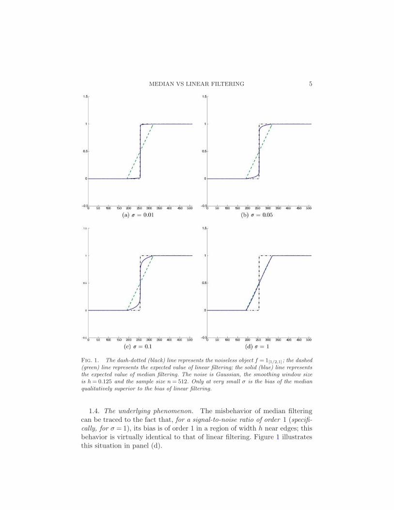
Fig. 1. The dash-dotted (black) line represents the noiseless object f = 1[1/2,1]; the dashed(green) line represents the expected value of linear filtering; the solid (blue) line representsthe expected value of median filtering. The noise is Gaussian, the smoothing window sizeis h = 0.125 and the sample size n = 512. Only at very small σ is the bias of the medianqualitatively superior to the bias of linear filtering.

1.4. The underlying phenomenon. The misbehavior of median filteringcan be traced to the fact that, for a signal-to-noise ratio of order 1 (specifi-

cally, for σ = 1), its bias is of order 1 in a region of width h near edges; thisbehavior is virtually identical to that of linear filtering. Figure 1 illustratesthis situation in panel (d).


However, the figure also illustrates, in panels (a), (b), (c), another phe-nomenon: for very low noise levels σ, that is, very high signal-to-noise ratios,the bias of the median behaves dramatically differently than the bias of lin-ear filtering. In particular, the bias is not large over an interval comparableto the window width, but only over a much smaller interval. In fact, asσ→ 0, the bias vanishes away from the edge. We call this the:

True hope of median filtering. At very low noise levels, medianfiltering can dramatically outperform linear filtering.

At first glance this seems utterly useless: why should we care to removenoise when there is almost no noise? On reflection, a useful idea emerges.Suppose we filter in stages, at the first stage using a relatively narrow windowwidth—much narrower than we would ordinarily use in a one-stage process—and at the second stage using a somewhat wider window width. The resultmay well achieve the noise reduction of the combined two-stage smoothingwith much smaller bias near edges.

Heuristic of iterated median filtering. Iterated median filtering,in which the data are first median-filtered lightly, at a fine scale, followedby a coarse-scale median filter, may outperform linear filtering.

Note that the same idea, applied to linear filtering, would achieve little.The composition of two linear filters can always be achieved by a singlelinear filter with appropriate kernel. And such weights do not change thequalitative effect of edges.

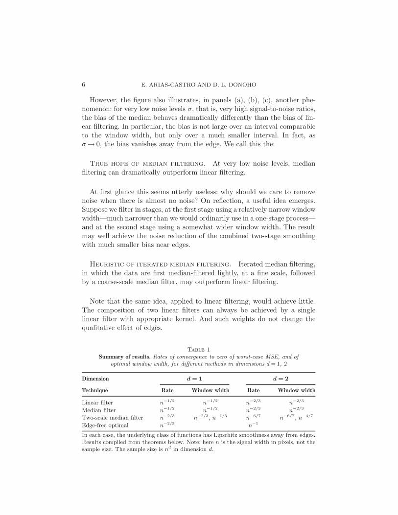
Table 1

Summary of results. Rates of convergence to zero of worst-case MSE, and ofoptimal window width, for different methods in dimensions d = 1, 2

Dimension d = 1 d = 2

Technique Rate Window width Rate Window width

Linear filter n−1/2 n−1/2 n−2/3 n−2/3

Median filter n−1/2 n−1/2 n−2/3 n−2/3

Two-scale median filter n−2/3 n−2/3, n−1/3 n−6/7 n−6/7, n−4/7

Edge-free optimal n−2/3 n−1

In each case, the underlying class of functions has Lipschitz smoothness away from edges.Results compiled from theorems below. Note: here n is the signal width in pixels, not thesample size. The sample size is nd in dimension d.


1.5. Results of this paper. Table 1 compiles the worst-case risk rates forlinear filtering, median filtering and two-scale median filtering over piece-wise Lipschitz function classes. The last line displays the minimax rates forLipschitz functions without discontinuities. Note that the rates would be thesame for classes of functions with higher degree of smoothness away from theedges—indeed, the three filtering methods considered here have worst-caserisk of same order of magnitude as their MSE for a simple step function suchas f(x) = 1x>1/2 in dimension d= 1.

Notice also that, in dimension d= 1 our two-scale median filtering achievesthe minimax rate for edge-free Lipschitz function classes. This is not the casein dimension d= 2, where other methods are superior [5, 21].

1.6. Iterated medians. As mentioned above, in the late 1960s Tukey al-ready proposed the use of iterated medians, although the motivations re-mained unclear to many at the time. In his proposals, different scales wereinvolved at different iterations, although the scales were relatively similarfrom the current viewpoint.

Significantly, iterated median filtering converges in some sense to MeanCurvature Motion (MCM), a popular PDE-based technique. In fact, thereis a wider link connecting PDE-based methods and iterative filtering; inparticular, iterated linear filtering converges to the Heat equation. See, forexample, [7, 8, 15]. Although MCM is highly nonlinear and hard to analyze,the heuristic above gives a hint that MCM might improve on linear filtering.

1.7. Prior literature. Several papers analyze the performance of medianfiltering numerically using simulations. For example, in [17], the authorsderive exact formulas for the distribution of the result of applying medianfiltering to a simple noisy edge like f0, and use computer-intensive simula-tions to provide numerical values. A similar approach is found in [19].

Closer to the present paper, [20] compares linear filtering and median fil-tering in the context of smooth functions and shows that they have minimaxrates of same order of magnitude. We will show here that the same holdsfor functions with discontinuities.

An extensive, but unrelated, body of literature explores the median’sability to suppress outliers, for example, [13] and also [28], which considerthe case of smoothing a one-dimensional signal corrupted with impulsivenoise. Using a similar framework, Donoho and Yu [12] study a pyramidalmedian transform.

1.8. Contents. In Sections 2 and 3, we consider one-dimensional and two-dimensional signals, respectively, in the constant-noise level case. In Section4 we consider per-pixel noise level tending to 0. In Section 5, we introduce a


two-scale median filtering and formulate results quantifying its performance.The proofs are postponed to the latter sections.

Though our results can be generalized to higher-dimensional signals andother smoothness classes, and can accommodate more sophisticated kernels,we choose not to pursue such extensions and generalizations here.

1.9. Notation. Below, we denote comparable asymptotic behavior of se-quences (an), (bn) ∈ R

N using an ≍ bn, meaning that the ratio an/bn isbounded away from 0 and ∞ as n becomes large.

2. Linear filtering and median filtering in dimension 1. Consider themodel (1.1) introduced in the Introduction for the case of dimension 1 (d=1). We now explicitly define the smoothness class of interest.

Definition 2.1. The local Lipschitz constant of the function f at x is

Lipx(f) = limsupε→0

sup|y−x|≤ε,y 6=x

|f(y)− f(x)||y − x| .

A function f : [0,1] 7→ R will be called essentially local Lipschitz if the es-sential supremum of the local Lipschitz constant on [0,1] is finite.

The function x1x>1/2(x) is essentially local Lipschitz but not Lipschitz;it has a local Lipschitz constant ≤ 1 almost everywhere on [0,1], but jumpsacross the line x= 1/2. More generally, piecewise polynomials without con-tinuity constraints at piece boundaries are essentially local Lipschitz and yetneither Lipschitz nor continuous.

Definition 2.2. Fix N ≥ 1 and β > 0. The class of punctuated-Lipschitz

functions pLip = pLip(β,N) is the collection of functions f : [0,1] 7→ [0,1]with local Lipschitz constant bounded by β on the complement of somefinite set (xi)

Ni=1 ⊂ (0,1).

Theorem 2.1. Assume Ψ has mean 0 and finite variance. Then,

infh>0

Rn(Lh;pLip)≍ n−1/2, n→∞.

This result can be proven using standard bias-variance trade-off ideas, andneeds only simple technical ingredients such as uniform bounds on functionsand derivatives. We explain in Section 7 that it can be inferred from existingresults, but then proceed to give a proof; this proof sets up a bias-variancetrade-off framework suitable for several less elementary situations whichcome later.


To analyze the behavior of median filtering, we must obtain uniformbounds on the stochastic behavior of empirical quantiles; these are laid outin Section 15 below. To enable such bounds, we make the following assump-tions on the noise distribution Ψ:

[Shape] Ψ has density ψ with respect to the Lebesgue measure on R, with

ψ unimodal, continuous and symmetric about 0.[Decay] ζ(Ψ) := sups > 0 :ψ(x)(|x| + 1)s is bounded> 1.

Note that the normal, double-exponential, Cauchy and uniform distribu-tions centered at 0 all satisfy both [Shape] and [Decay]. These conditionspermit an efficient proof of the following result—see Section 8; the conditionscould probably be relaxed considerably, leading to a more difficult proof.

Theorem 2.2. Assume Ψ satisfies [Shape] and [Decay]. Then,

infh>0

Rn(Mh;pLip)≍ n−1/2, n→∞.

For piecewise Lipschitz functions corrupted with white additive Gaus-sian noise (say) having constant per-pixel noise level, Theorems 2.1 and 2.2show that linear filtering and median filtering have risks of same order ofmagnitude Rn ≍ n−1/2—the same holds for any noise distribution Ψ withfinite variance satisfying [Shape] and [Decay]. In that sense, the Median folktheorem is contradicted.

The proof shows that the optimal order of magnitude for the width hn

of the median smoothing window obeys hn ≍ n−1/2—again the same as inlinear filtering.

3. Linear filtering and median filtering in dimension 2. Consider mod-el (1.1) of the Introduction in the case of dimension 2 (d= 2); our “signals”are now digital images. Our smoothness class here is a class of cartoon im-

ages, which are piecewise functions that are smooth except for discontinuitiesalong smooth curves—see also [6, 9, 21].

Just as in d= 1, we have the notion of local Lipschitz constant. In d= 2,the function x1x>1/2(x, y) is essentially local Lipschitz but not Lipschitz;this has a local Lipschitz constant bounded by 1 almost everywhere, butthe function jumps as we cross the line x = 1/2. More generally, cartoonimages have the same character: essentially local Lipschitz and yet neitherLipschitz nor continuous. Such cartoon images, of course, have jumps alongcollections of regular curves; we formalize such collections as follows.

Definition 3.1. A finite collection of rectifiable planar curves will becalled a complex. Fix λ > 0 and let Γ = Γ(λ) denote the class of rectifiablecurves in [0,1]2 with length at most λ. Let C(N,λ) denote the collection ofcomplexes composed of at most N curves from Γ(λ).


Definition 3.2. Fix N ≥ 1 and β > 0. The class of curve-punctuated

Lipschitz functions cpLip = cpLip(λ,β,N) is the collection of functionsf : [0,1]2 7→ [0,1] having local Lipschitz constant bounded by β on the com-plement of a C(N,λ)-complex.

Informally, such functions are “locally Lipschitz away from edges” andindeed can be viewed as models of “cartoons.” We prove the next two resultsin Sections 10 and 11, respectively.

Theorem 3.1. Assume Ψ has mean 0 and variance 1. Then

infh>0

Rn(Lh;cpLip) ≍ n−2/3, n→∞.


infh>0

Rn(Mh;cpLip)≍ n−2/3, n→∞.

The situation parallels the one-dimensional case. In words, for cartoon im-ages corrupted with white additive noise with constant per-pixel noise level,linear filtering and median filtering have risks of same order of magnitudeRn ≍ n−2/3. Again, the Median folk theorem is contradicted.

The proofs show that the width of the optimal smoothing window foreither type of smoothing is ≍ n−2/3.

4. Linear filtering and median filtering with negligible per-pixel noise

level. The analysis so far assumes that the noise level is comparable to thesignal level.

For very low-noise-per-pixel level and discontinuities well-separated fromthe boundary and each other, the situation is completely different: the Me-

dian folk theorem holds true.

Preliminary remark. We will see in Sections 9 and 12 that, both in di-mensions d= 1 and d= 2, linear filtering does not improve on no-smoothingif σnn

1/2 =O(1), while median filtering improves on no-smoothing if σnn→∞. In Theorems 4.1 and 4.2 below we therefore exclude the situation σnn=O(1).

Definition 4.1. The finite point set (xi)Ni=1 ⊂ [0,1] is called well-separated

with separation constant η > 0 if (i) each point is at least η-separated fromthe boundary 0,1:

min(xi,1− xi)≥ η ∀iand (ii) each point is at least η-separated from every other point:

|xj − xi| ≥ η ∀i, j.


Definition 4.2. Let sep-pLip = sep-pLip(η,β,N) denote the class offunctions in pLip(β,N) which have local Lipschitz constant ≤ β on thecomplement of some η-well-separated set (xi)

Ni=1.

Theorem 4.1. Let Ψ satisfy [Shape] and [Decay] and let the per-pixel

noise level tend to zero with increasing sample size, σ = σn → 0 as n→∞,

with σnn→∞. Then,

infh>0

Rn(Mh; sep-pLip) = o

(

infh>0

Rn(Lh; sep-pLip)

)

, n→∞.

The proof is in Section 9, where we provide more explicit bounds for therisks of linear and median filtering.

In dimension d= 2, we again have that for negligible per-pixel noise levelthe Median folk theorem holds true. To show this, we need the hypothesisthat the discontinuity curves are well-separated from the boundary, and fromeach other.

Definition 4.3 (Well-separated complex). Let d(A,B) denote Hauss-dorff distance between compact sets A and B. A complex C = (γi) of recti-fiable curves in [0,1]2 is said to be well-separated with separation parameterη > 0, if (i) the curves are separated from the boundary of the square:

d(γi,bdry[0,1]2)≥ η ∀iand (ii) the curves are separated from each other:

d(γi, γj)≥ η ∀i, j.

We also need that the curves are well-separated from themselves (i.e., donot loop back on themselves). Formally, we need the condition

Definition 4.4 (C2 Chord-arc curves). Fix parameters λ,κ, θ. Let Γ2 =Γ2(λ,κ, θ) be the collection of planar C2 curves γ with curvature boundedby κ and chord-arc ratio bounded by θ:

∀s < tt− s

|γ(t)− γ(s)| ≤ θ andlength(γ)− t+ s

|γ(t)− γ(s)| ≤ θ.

Related classes of curves appear in, for example, Section 5.3 of [21]. Note thatcurves with bounded chord-arc ratio appear in harmonic analysis related topotential theory, for example, [32].

Definition 4.5. Let sep-cpLip = sep-cpLip(λ, θ,κ, η, β,N) be the col-lection of curve-punctuated Lipschitz functions with local Lipschitz constantbounded by β on the complement of an η-well-separated C(N,λ)-complexof κ, θ chord-arc curves.


For an example, let f = 1D, where D is the disk of radius 1/4 centered at(1/2,1/2). Then the exceptional complex C = γ1, where

γ1(θ) = (12 ,

12)′ + 1

4(cos(θ), sin(θ))′, θ ∈ [0,2π).

For this example, f ∈ sep-cpLip with parameters

N ≥ 1, λ≥ π

2, β ≥ 0, θ ≥ π

2, κ≥ 4, η ≤ 1

4 .

As this example shows, we may choose parameters so that the classes Γ andsep-cpLip are nonempty. In the sequel, we assume this has been done, sothat sep-cpLip contains the f just given.

Theorem 4.2. Assume Ψ satisfies [Shape] and [Decay] and that the

per-pixel noise level tends to zero with increasing sample size, σ = σn → 0as n→∞, with σnn→∞. Then,

infh>0

Rn(Mh; sep-cpLip) = o

(

infh>0

Rn(Lh; sep-cpLip)

)

, n→∞.

The proof is in Section 12.

5. Iterated and two-scale median filtering. Iterated (or repeated) me-dian filtering applies a series of median filters Mh1,...,hm[Yn] ≡Mhm · · · Mh1 [Yn]. That is, median filtering with window size h1 is first applied, thenmedian filtering with window size h2 is applied to the resulting signal, andso on. In the 1970s Tukey advocated such compositions of medians in con-nection with d = 1 signals, for example, applying medians of lengths 3, 5,and 7 in sequence—possibly, along with other operations, including linearfiltering. Here we are interested in much longer windows than Tukey, in factin windows that grow large as n increases.

Tukey also advocated the iteration of medians until convergence—his so-called “3R” median filter applies running medians of three repeatedly untilno change occurs. The mathematical study of repeated medians Mh1,...,hm

is a challenging endeavor, however, because of the strong dependency thatmedian filtering introduces with every pass, though [3, 4] attempt to carryout just such studies, in the situation where there is only noise and no signal.See also Rousseeuw and Bassett [29].

Here, inspired by the intuition supplied in Figure 1 and by the results ofthe previous section, we consider two-scale median filtering. The first passaims at increasing the signal-to-noise ratio, so the second pass can exploitthe promising characteristics of median filtering at high signal-to-noise ratio.

We describe the process in dimension d. For h > 0, consider the squares

Bhk = [k1nh+ 1, (k1 + 1)nh)× · · · × [kdnh+ 1, (kd + 1)nh),

where k = (k1, . . . , kd) ∈ Nd with 0 ≤ kj < 1/h. Fix 0< h1 <h2 < 1 and define

Mh1,h2[Yn] as follows:


1. For k = (k1, . . . , kd) ∈ Nd with 0 ≤ kj < 1/h1, define

Y h1n (k) = MedianYn(i) : i ∈Bh1

k;

thus Y h1n is a coarsened version of Yn.

2. For i ∈Bh1k

, define

Mh1,h2[Yn](i) =Mh2 [Yh1n ](k).

In words, we apply median filtering to the coarse-scale version Y h1n and get

back the fine-scale version by crude piecewise interpolation. The followingresults, for d= 1,2, respectively, are proven in Sections 13 and 14.


inf0<h1<h2

Rn(Mh1,h2; sep-pLip) ≍ n−2/3, n→∞.


inf0<h1<h2

Rn(Mh1,h2; sep-cpLip) ≍ n−6/7, n→∞.

Compare Theorems 5.1 and 5.2 with Theorems 2.2 and 3.2, respectively. Indimension d= 1, the rate improves from O(n−1/2) to O(n−2/3); in dimensiond = 2, from O(n−2/3) to O(n−6/7). Hence, with carefully chosen windowsizes, our two-scale median filtering outperforms linear filtering. The optimalchoices are h1 ≍ n−2/3 and h2 ≍ n−1/3 for d= 1; h1 ≍ n−6/7 and h2 ≍ n−4/7

for d= 2.Though this falls short of proving that indefinitely iterated median filter-

ing of the sort envisioned by Tukey dramatically improves on linear filteringor that the PDE folk theorem is true for Mean Curvature Motion, it certainlysuggests hypotheses for future research in those directions.

6. Tools for analysis of medians. Before proceeding step-by-step withproofs of the theorems announced above, we isolate some special facts aboutmedians which are used frequently and which ultimately drive our analysis.

6.1. Elementary properties. Let Medn(·) denote the empirical median ofn numbers. We make the following obvious but essential observations:

• Monotonicity. If xi ≤ yi, i= 1, . . . , n,

Medn(x1, . . . , xn) ≤Medn(y1, . . . , yn).(6.1)

• Lipschitz mapping.

|Medn(x1, . . . , xn)−Medn(y1, . . . , yn)| ≤ nmaxi=1

|xi − yi|.(6.2)


6.2. Bias bounds. Since Huber [18] the median is known to be optimallyrobust against bias due to data contamination. Such robustness is essentialto our analysis of the behavior of median filtering near edges. In effect, datacontributed by the “other side” of an edge act as contamination that themedian can optimally resist.

Consider now a composite dataset of n + m points made from xi, i =1, . . . , n, yi, i = 1, . . . ,m. Think of the y’s as “bad” contamination of the“good” xi which may potentially corrupt the value of the median. Howmuch damage can the y’s do? Equation (6.1) yields the mixture bounds

Medn+m(x1, . . . , xn,−∞, . . . ,−∞) ≤ Medn+m(x1, . . . , xn, y1, . . . , ym)(6.3)

≤ Medn+m(x1, . . . , xn,∞, . . . ,∞).

Observe that if m<n, then the median of the combined sample cannot belarger than the maximum of the x’s nor can it be smaller than the minimumof the x’s:

Medn+m(x1, . . . , xn,−∞, . . . ,−∞)≥ min(x1, . . . , xn)

and

Medn+m(x1, . . . , xn,∞, . . . ,∞)≤ max(x1, . . . , xn).

Generalizing this observation leads to bias bounds employing the empir-ical quantiles of x1, . . . , xn. Let Fn(t) = n−1#i :xi ≤ t be the usual cu-mulative distribution function of the numbers (xi), and let F−1

n denote theempirical quantile function. Set ε=m/(m+n) and suppose ε ∈ (0,1/2). Asin [18], we bound the median of the combined sample by the quantiles ofthe “good” data only:

F−1n

(

1/2− ε

1− ε

)

≤Medn+m(x1, . . . , xn, y1, . . . , ym) ≤ F−1n

(

1/2

1− ε

)

.(6.4)

This inequality will be helpful later, when the combined sample correspondsto all the data within a window of the median filter, the “good” data cor-respond to the part of the window on the “right” side of an edge, and the“bad” data correspond to the part of the window on the “wrong” side of theedge.

6.3. Variance bounds for uncontaminated data. The stochastic proper-ties of the median are also crucial in our analysis; in particular we needbounds on the variance of the median of “uncontaminated” samples, that

is, of the samples (Zi)mi=1, Zi

i.i.d.∼ Ψ. The following bounds on the variance ofempirical medians behave similarly to expressions for variances of empiricalaverages.


Lemma 6.1. Suppose Ψ satisfies [Shape] and [Decay]. Then, there are

constants C1,C2 depending only on ζ(Ψ), such that

C1

m≤ E[Medm(Z1, . . . ,Zm)2] ≤ C2

m, m= 1,2, . . . .

Proof. In Section 15, we prove Lemma 15.1 which states that [Shape]and [Decay] imply a condition due to David Mason, allowing us to applyProposition 2 in [23].

We also need to analyze the properties of repeated medians (mediansof medians). Borrowing ideas of Rousseeuw and Bassett [29], we prove thefollowing in Section 15.

Lemma 6.2. Assume Ψ satisfies [Shape] and [Decay], and considerZ1, . . . ,Zm a sample from Ψ. Let Ψm denote the distribution of m1/2 MedianZ1,. . . ,Zm. Then, for all m, Ψm satisfies [Shape] and [Decay]. More precisely,

there is a constant C such that, for m large enough, ψm(x)(1+ |x|)4 ≤C for

all x.

6.4. Variance of empirical quantiles, uncontaminated data. Because ofthe bias bound (6.4) it will be important to control not only the empiricalmedian, but also other empirical quantiles besides p= 1

2 .Let Zm,p denote the empirical p-quantile of Z1, . . . ,Zm, a sample from

Ψ. That is, with Z(1), . . . ,Z(m) denoting order statistics of the sample, and0< p< 1,

Zm,p ≡Z(1+⌊mp⌋).

Lemma 6.3. Fix ζ > 1. Let Ψ satisfy [Shape] and [Decay]. Define

α=

5ζ − 3

4ζ − 4, if ζ > 3,

ζ

ζ − 1, if ζ ≤ 3.

(6.5)

There is a constant C > 0 such that, for all sufficiently large positive integer

m and p ∈ (2α/m,1 − 2α/m),

E[Z2m,p]≤C(p(1− p))−2α+2.

Proof. Again noting Lemma 15.1, we are entitled to apply Proposition2 in [23]. We then invoke Lemma 15.2.

In words, provided that we do not consider quantiles p very close to theextremes 0 and 1, the variance is well-controlled. The rate at which thevariance blows up as p→ 0 or 1 is ultimately determined by the value ofζ > 1 and will be of crucial significance for some bounds below.


6.5. MSE lower bound for contaminated data. As a final key ingredi-ent in our analysis, we develop a simple lower bound on the mean-squaredisplacement of the empirical median of contaminated data. Let

µn,m,∆ ∼ Medn+m(Z1, . . . ,Zn,Zn+1 + ∆, . . . ,Zn+m + ∆).

In words this is the empirical median of n+m values, the first n of whichare “good” data with median 0, and the last m of which are contaminated,having median ∆. For ∆> 0 and ε ∈ (0,1), define the mixture CDF

Fε,∆(·) = (1− ε)Ψ(·) + (1− ε)Ψ(· −∆).(6.6)

Let µ= µ(ε,∆) be the corresponding population median:

µ= F−1ε,∆(1

2).

Actually, µ(ε,∆) is almost the population median of the empirical medianµn,m,∆. More precisely, we have the following lemma.

Lemma 6.4. For ε=m/(n+m),

Pµn,m,∆ ≥ µ(ε,∆) ≥ 1/2.

Proof. For all a ∈ R

Pµn,m,∆ < a = P

n∑

j=1

Zj < a+n+m∑

j=n+1

Zj < a−∆ ≥ (n+m)/2

.

Applying a result of Hoeffding [35], page 805, Inequality 1, we get that, fora≤ µ(ε,∆), the right-hand side is bounded by

PBin(n+m,Fε,∆(a)) ≥ (n+m)/2 ≤ 1/2.

For each fixed ∆> 0, increasing contamination only increases the popu-lation median:

µ(ε,∆) is an increasing function of ε ∈ (0,1/2).(6.7)

Combining the last two observations, we have the MSE lower bound

Eµ2n,m,∆ ≥ µ(ε0,∆)2/2, ε0 <m/(n+m).(6.8)

7. Proof of Theorem 2.1. We now turn to proofs of our main results.In what follows, C stands for a generic positive constant that depends onlyon the relevant function class and the distribution Ψ; its value may changefrom appearance to appearance. Also, to simplify the notation we use W(i) ≡W[n,h](i), Lh(i) ≡Lh[Yn](i) and so on. We also write F1 in place of pLip.


7.1. Upper bound. Fix f ∈ F1. Let x1, . . . , xN ∈ (0,1) denote the pointswhere f is allowed to be discontinuous. Here and throughout the rest of thepaper we assume that h≥ 1/n. Indeed, if to the contrary h < 1/n, then forall i ∈ In, W(i) = i and so Rn(Lh;f) = σ2 ≍ 1.

We will demonstrate that

R(Lh;F1) ≤C

(

h+1

nh

)

.(7.1)

Minimizing the right-hand side as a function of h≥ 1/n gives hn = n−1/2,which implies our desired upper bound:

R(Lh;F1)≤Cn−1/2.(7.2)

This upper bound may also be obtained from existing results, because F1

is included in a total-variation ball. Indeed,

‖f‖BV ≤ 2β +N,

so, in an obvious notation F1 ⊂ BV (2β + N). From standard results onestimation of functions of bounded variation in white noise—[10, 21]—weknow that

infh>0

R(Lh;BV (ν))≤ ν · n−1/2,

which implies (7.2). Nevertheless, we spell out here an argument based onbias-variance trade-off, because this sort of trade-off will be used again re-peatedly below.

Write the mean-squared error as squared bias plus variance: Rn(Lh;f) =B2 + V , where

B2 =1

n

n∑

i=1

(E[Lh(i)]− f(i/n))2 and V =1

n

n∑

i=1

var[Lh(i)].

For the variance, since the Yn(j) : j ∈ In are pairwise uncorrelated andtheir variance is equal to σ2, we have

var[Lh(i)] =σ2

#W(i)≤ σ2

nh.

Therefore,

V ≤ σ2

nh.(7.3)

For the bias, recall that E[Yn(j)] = f(j/n) for all j ∈ In, so

E[Lh(i)] =1

#W(i)

∑

j∈W(i)

f(j/n).

Now consider separately cases where i is “near to” and “far from” the dis-continuity. Specifically, define:


• Near: ∆ = i ∈ In :mins |i/n − xs| ≤ h—in words, ∆ is the set of pointswhere the smoothing window does meet the discontinuity.

• Far: ∆c = i ∈ In :mins |i/n− xs|> h—∆c is the set of points where thesmoothing window does not meet the discontinuity.

Near the discontinuity, use the fact that as f takes values in [0,1],

|E[Lh(i)]− f(i/n)| ≤ 1.(7.4)

Far from the discontinuity, we apply a sharper estimate that we nowdevelop. Let i ∈ ∆c and consider j ∈ W(i). The local Lipschitz constantbound β gives

|f(j/n)− f(i/n)| ≤ h supx∈[i/n,j/n]

Lx(f)≤ βh,(7.5)

which implies

|E[Lh(i)]− f(i/n)| ≤ βh, i ∈ ∆c.(7.6)

Combining (7.4) and (7.6), we bound the squared bias by

B2 ≤ #∆c

nβ2h2 +

#∆

n.(7.7)

The number of “near” terms obeys 0≤ #∆ ≤N(2nh+1), and of course thefraction of “far” terms obeys #∆c/n≤ 1, so we get

B2 ≤ β2h2 + 2Nh+N/n≤Ch,(7.8)

since h≥ 1/n; we may take C = (β2 + 3N).Hence, R(Lh;f) ≤ C(h + 1/(nh)), and this bound does not depend on

f ∈F1, so (7.1) follows.

7.2. Lower bound. Let f be the indicator function of the interval [1/2,1].Then f ∈F1 for all N ≥ 1 and β > 0.

For the variance, since #W(i) ≤ 3nh, we have

V ≥ σ2

3nh.

For the squared bias, we show that the pointwise bias is large near thediscontinuity. For example, take n/2 − nh/2 ≤ i < n/2, so that f(i/n) = 0and therefore

|E[Lh(i)]− f(i/n)|= E[Lh(i)] =#j ∈W(i) : j/n≥ 1/2

#W(i).

Since #j ∈W(i) : j/n≥ 1/2 ≥ nh/2 and #W(i) ≤ 3nh, the pointwise biasexceeds 1/6:

|E[Lh(i)]− f(i/n)| ≥ nh/2

3nh≥ 1/6.


Therefore,

B2 ≥ #i ∈ In :n/2− nh/2 ≤ i < n/2n

(1/6)2 ≥Ch,

where C = 1/72 will do.Combining bias and variance bounds, we have for any choice of radius h,

Rn(Lh;f)≥C

(

h+1

nh

)

≥Cn−1/2.

8. Proof of Theorem 2.2. Now we analyze median filtering. The proofparallels that for Theorem 2.1 and uses the results of Section 6. Here too,we use abbreviated notation.

8.1. Upper bound. Fix f ∈F1. Let x1, . . . , xN ∈ (0,1) be the points wheref may be discontinuous. Without loss of generality, we again let h≥ 1/n.

We will show that

Rn(Mh;F1)≤C

(

h+1

nh

)

.(8.1)

As in the proof of Theorem 2.1, picking hn = n−1/2 in (8.1) implies ourdesired upper bound, namely:

infh>0

Rn(Mh;F1)≤Cn−1/2.

To get started, we invoke the monotonicity and Lipschitz properties ofthe median (6.1)–(6.2), yielding

|Mh(i)− f(i/n)| ≤ maxj∈W(i)

|f(j/n)− f(i/n)|+ σ|Z(i)|,

where Z(i) = MedianZn(j) : j ∈W(i).Near the discontinuity, we again observe that since f takes values in [0,1],

we have

maxj∈W(i)

|f(j/n)− f(i/n)| ≤ 1

for all i ∈ In, and so

|Mh(i)− f(i/n)| ≤ 1 + σ|Z(i)| ∀i ∈ In.(8.2)

Now consider the set ∆c = i ∈ In :mins |i/n− xs|> h far from the dis-continuity. Using (7.5), we get

|Mh(i)− f(i/n)| ≤ βh+ σ|Z(i)| ∀i ∈ ∆c.(8.3)

Using (8.2) and (8.3), we get

Rn(Mh;f)≤ #∆c

nβ2h2 +

#∆

n+

1

n

n∑

i=1

E[Z(i)2].(8.4)


The term on the far right is a variance term, which can be handled usingLemma 6.1 at sample size m= #W(i) ≥ nh, yielding variance V ≤C/(nh).The bias terms involve #∆ and #∆c and are completely analogous to thecase of linear filtering and are handled just as at (7.8), using 0 ≤ #∆ ≤N(2nh + 1). We obtain Rn(Mh;f) ≤ C(h + 1/(nh)). Since this does notdepend on f ∈ F1, (8.1) follows.

8.2. Lower bound. Let f be the indicator function of the interval [1/2,1].Surely, f ∈F1 for any N ≥ 1 and β > 0.

For i ∈ ∆c

|Mh(i)− f(i/n)| = σ|Z(i)|,so that, by Lemma 6.1,

E[(Mh(i)− f(i/n))2]≥C1

nh.(8.5)

Therefore,

1

n

∑

i∈∆c

E[(Mh(i)− f(i/n))2]≥C1

nh.

For i ∈ ∆, we view the window as consisting of a mixture of “good” data,on the same side of the discontinuity as i together with “bad” data, on theother side. Thus

|Mh(i)− f(i/n)| = σ|Kn(i)|,where, with w(i) = #W(i) ≍ nh, and

ρ(i) = #j : j ∈W(i) and on the same side of the discontinuitywe have

Kn(i) ∼ MedianZ1, . . . ,Zρ(i)w(i),Z1+ρ(i)w(i) + 1/σ, . . . ,Zw(i) + 1/σ.This is exactly a median of contaminated data as discussed in Section6.5, with ∆ = 1/σ, m + n = w(i), n = ρ(i)w(i) and ε = 1 − ρ(i). InvokingLemma 6.4 with µi = µ(1 − ρ(i),1/σ), applying (6.8) for ε0 = 1/5 and set-ting C = σ2µ2(1/5,1/σ)/2, we have

E[(Mh(i)− f(i/n))2]≥C ∀i such that ρ(i) ≤ 4/5.(8.6)

Since #i :ρ(i) ≤ 4/5 ≍ nh, we get

1

n

∑

i∈∆

E[(Mh(i)− f(i/n))2]≥Ch.

Combining pieces, we get for any choice of h

Rn(Mh;f)≥C

(

h+1

nh

)

≥C · n−1/2,

which matches the upper bound.


9. Proof of Theorem 4.1. We turn to the setting of Section 4: asymptot-ically negligible noise per pixel: σ = σn = o(1).

9.1. Linear filtering. By just carrying the variance term in Section 7 andcomparing with the no-smoothing rate, we immediately see that

R(Lh; sep-pLip)≍ σnn−1/2 ∧ σ2

n.

Hence, linear filtering improves on no-smoothing if, and only if, σnn1/2 →∞.

9.2. Upper bound for median filtering. We refine the argument from Sec-tion 8 in the case where the discontinuities are well-separated. Let F+

1 =sep-pLip as defined in Section 5. Note that (9.7) will be used in the proofof Theorem 5.1.

Assuming n > 2/η, choose h ∈ [1/n, η/2). Since median filtering is localand the discontinuities are η-separated, we may assume that f only hasN = 1 discontinuity point x1.

Far from the discontinuity, at i ∈ ∆c, we use (8.2) and Lemma 6.1 to get

E[(Mh(i)− f(i/n))2] ≤C

(

h2 +σ2

n

nh

)

, i ∈∆c;(9.1)

note that σn is now nonconstant.Near the discontinuity, we now take more seriously the viewpoint that the

window contains “good” data (on the same side of the discontinuity) and“bad” data (on the other side) and we bound the MSE more carefully thanbefore.

So take i ∈ ∆. Define the “good” subset G(i)—the subset of the windowon the same side of the discontinuity as i—by

G(i) =

W(i)∩ [nx1, n], i/n > x1,W(i)∩ [1, nx1), i/n < x1.

(9.2)

Let ρ(i) = #G(i)/#W(i) and ε(i) = 1− ρ(i). The window W(i) provides anε-contaminated sample in the sense of Huber [18].

By the contamination bias bound (6.4), Mh(i) lies between the 1/2−ε1−ε =

(2ρ(i)−1)/(2ρ(i)) and 12(1−ε) = 1/(2ρ(i)) quantiles of Yn(j) : j ∈ G(i). Also,

as in (7.5), we have

|f(j/n)− f(i/n)| ≤ βh ∀j ∈ G(i),

so the quantiles of these “good data” Yn(j) : j ∈ G(i) are small perturba-tions of the quantiles of corresponding zero-median data Zn(j) : j ∈ G(i).Let Qn(i) denote the maximum absolute value of the empirical (2ρ(i) −1)/(2ρ(i)) and 1/(2ρ(i)) quantiles of Zn(j) : j ∈ G(i). By (6.2) and (6.4)

|Mh(i)− f(i/n)| ≤ βh+ σnQn(i).(9.3)


We combine (9.3) with (8.2) and Lemma 6.1 to get

E[(Mh(i)− f(i/n))2] ≤CE[(1 + σ2nZ(i)2)∧ (β2h2 + σ2

nQn(i)2)]

≤C(1 + σ2nE[Z(i)2]) ∧ (β2h2 + σ2

nE[Qn(i)2])

≤C(h2 + 1∧ σ2nE[Qn(i)2]),

where for the last inequality we used Lemma 6.1 together with h≥ 1/n, andthe fact that a∧ (b+ c) ≤ (a∧ b) + c for any a, b, c≥ 0.

Recalling Section 6.4, let Zm,p denote the empirical p-quantile of Z1, . . . ,Zm,a sample from Ψ. Because Ψ is symmetric about 0, |Qn(i)| is stochasti-cally majorized by 2|Zm(i),p(i)|, with m(i) = #G(i) = ρ(i)#W(i) and p(i) =1/(2ρ(i)). Hence

E[Qn(i)2]≤ 4E[Z2m(i),p(i)].(9.4)

Using (9.4) and Lemma 6.3, we obtain, for i ∈∆,

E[(Mh(i)− f(i/n))2]≤C(h2 + 1∧ σ2n(p(i)(1− p(i)))−2α+2).

Therefore,

Rn(Mh;f)≤C

(

h2 +σ2

n

nh+

1

n

∑

i∈∆

1∧ σ2n(p(i)(1− p(i)))−2α+2

)

.(9.5)

We focus on the last term on the right-hand side.Let δ(i) = |i/n− x1|; since i ∈∆, δ(i) ≤ h. We have

ρ(i) =[nδ(i)] + [nh] + 1

2[nh] + 1≥ 1

2+C

δ(i)

h.

So there is a constant C > 0 such that

p(i)≤ 1−Cδ(i)/h ∀i ∈ ∆.(9.6)

Note that we always have p(i) ≥ 1/2.Therefore

1

n

∑

i∈∆

1∧ σ2n(p(i)(1− p(i)))−2α+2 ≤ C

1

n

∑

i∈∆

1∧ σ2n(δ(i)/h)−2α+2

≤ Ch1

nh

nh∑

i=1

1 ∧ σ2n(i/(nh))−2α+2

≤ Ch

∫ 1

01∧ σ2

ns−2α+2 ds=Chνn

with

νn =

σ2n, if ζ > 3,

σ2n log(1/σn), if ζ = 3,σζ−1

n , if ζ < 3.


Combining pieces gives

Rn(Mh;f)≤C

(

h2 +σ2

n

nh+ hνn

)

.(9.7)

Optimizing the right-hand side over h, we get

Rn(Mh;f)≤C(ν1/2n ∨ σ1/3

n n−1/6) · σnn−1/2 = o(σnn

−1/2).

This bound improves on no-smoothing if σnn→∞.

9.3. Lower bound for median filtering. A lower bound is not needed toprove Theorem 4.1. However, we will use the following lower bound in theproof of Theorem 5.1.

Let f be the indicator function of the interval [1/2,1]. A lower bound isobtained by using the arguments in Section 8.2, but this time carrying σn

along and noticing that µ(ε,∆) is increasing in ∆. One gets

Rn(Mh;f)≥C

(

hσ2n +

σ2n

nh

)

.(9.8)

This bound matches the upper bound, for example, when ζ > 3 and σnn1/4 →

∞. This is the setting that will arise in Section 13.

10. Proof of Theorem 3.1. We consider two-dimensional linear filtering.The structure of the argument parallels the one-dimensional case presentedin Section 7. The main difference involves counting points near to disconti-nuities.

10.1. Upper bound. We also write F2 in place of cpLip. Fix f ∈F2. Wecall γ1, . . . , γN ∈ Γ the curves where f may be discontinuous.

As before, we write MSE =B2 + V .Again, we may assume h ≥ 1/n. Since #W(i) ≥ (nh)2, we have V ≤

1/(nh)2.In the two-dimensional case, we define proximity to singularity as follows.

Write d(A,B) for Haussdorff distance between subsets A and B of the unitsquare:

• Far: Let ∆c = i ∈ I2n :mins d(i/n, γs)> h.

• Near: Let ∆ = i ∈ I2n :mins d(i/n, γs)≤ h.

Using the exact same arguments as in Section 7, we obtain the equivalentof (7.7):

B2 ≤ #∆c

n2β2h2 +

#∆

n2≤ β2h2 +

#∆

n2.


Lemma 16.1 provides an estimate for #∆ which, when used in the aboveexpression, implies B2 ≤Ch.

Thus, Rn(Lh;f)≤C(h+ 1/(nh)2). The right-hand side does not dependon f ∈F2, so

Rn(Lh;F2)≤C

(

h+1

(nh)2

)

.

Minimizing the right-hand side over h≥ 1/n gives h= n−2/3, yielding R(Lh;F2)≤Cn−2/3.

10.2. Lower bound. Fix 0< ζ < (1/2) ∧ (λ/4) and let f be the indicatorfunction of the axis-aligned square of sidelength ζ centered at (1/2,1/2),namely f = 1S where S = [1/2 − ζ/2,1/2 + ζ/2] × [1/2 − ζ/2,1/2 + ζ/2].Certainly, f ∈F2.

Again, the variance V ≥ 1/(3nh)2 . For the squared bias B2, we show thatthe pointwise bias is of order 1 near the discontinuity. For example, takei ∈ I

2n such that

i/n ∈ [1/2− ζ/2− h/2,1/2 − ζ/2]× [1/2− ζ/2,1/2 + ζ/2],

so that f(i/n) = 0 and therefore the bias obeys

|E[Lh(i)]− f(i/n)|= E[Lh(i)] =#j ∈W(i) : j ∈ nS

#W(i).

For such i, #W(i) ∩ nS is of order (nh)2, since the intersection of thedisc of radius h centered at i/n with S contains a square of sidelength Ch.Therefore, the bias is of order 1 for such i, and there are order n2h such i.Hence the squared bias B2 is at least of order h.

Combining pieces, we get for all h,

Rn(Lh;f)≥C ·(

h+1

(nh)2

)

≥C · n−2/3.

11. Proof of Theorem 3.2. The structure of the proof is identical to thecase of one-dimensional signals presented in Section 8. In the details, theonly significant difference is on computing the number of points away fromdiscontinuities. We use the same definitions ∆ and ∆c as in Section 8.

11.1. Upper bound. Fix f ∈ F2. We call γ1, . . . , γN ∈ Γ the curves wheref may be discontinuous. Again, we may assume h≥ 1/n.

Define ∆c = i ∈ I2n :mins d(i/n, γs)>h. Using the exact same arguments

as in Section 8, we obtain the equivalent of (8.4):

Rn(Mh;f)≤ #∆c

n2β2h2 +

#∆

n2+

1

n2

∑

i∈I2n

E[Z(i)2].


Lemma 16.1 provides an estimate for #∆ which, when used in the aboveexpression, leads to Rn(Lh;f)≤C(h+1/(nh)2). From there we conclude asin Section 10.1.

11.2. Lower bound. Let f ∈ F2 be the indicator function of a disc D.For i ∈ ∆c, the equivalent of (8.5) holds and together with Lemma 16.1

implies

1

n2

∑

i∈∆c

E[(Mh(i)− f(i/n))2]≥C1

(nh)2.

The equivalent of (8.6) holds as well and implies

1

n2

∑

i∈∆

E[(Mh(i)− f(i/n))2]≥C1

n2#i :ρ(i)≤ 4/5.

We now show that, for i/n ∈Dc such that δ(i) ≥ 1/n, ρ(i) ≤ 1/2+Cδ(i)/h.Let y ∈ ∂D be the closest point to i/n and L the tangent to ∂D at y. Ldivides B(i/n,h) into two parts A and B(i/n,h) ∩Ac, where i/n ∈ A. Wehave A= A0 ∪H , where H is the open half disc with diameter parallel toL that does not intersect ∂D. We have G(i) = I

2n ∩ nA, so that #G(i) ≤

#W(i)/2+#(I2n ∩nA0). A0 is contained within a rectangular region R withdimensions δ(i) by 2h and for any rectangular region, |R| ≤C|R|n2 +O(nh).Hence, since nδ(i) ≥ 1,

#(I2n ∩ nA0) ≤#(I2n ∩ nR)≤Chδ(i)n2.

Therefore, ρ(i)≤ 1/2 +Cδ(i)/h.We thus have

#i :ρ(i)≤ 4/5 ≥#i : 1/n≤ δ(i) ≤Ch.Let K = |x :d(x,∂D) ≤Ch|. We have nh≫ 1 so that

K ⊂⋃

i/n∈R

B(i/n,2/n),

which implies |K| ≤ C#i : δ(i) ≤ Ch/n2. By elementary calculus, |K| ≥Ch, so

#i :ρ(i)≤ 4/5 ≥Cn2h.

We obtain for all h

Rn(Mh;f)≥C

(

1

(nh)2+ h

)

≥Cn−2/3.

12. Proof of Theorem 4.2. We consider again median filtering in thenegligible-noise-per-pixel case of Section 4, this time in the two-dimensionalsetting.


12.1. Linear filtering. By just carrying the variance term in Section 10and comparing with the no-smoothing rate, we immediately see that

R(Lh; sep-cpLip)≍ σ2/3n n−2/3 ∧ σ2

n.

Hence, linear filtering improves on no-smoothing if, and only if, σnn1/2 →∞.

12.2. Upper bound for median filtering. We refine our arguments in thesetting of asymptotically negligible noise level σ = σn = o(1) with well-separated discontinuities. Let F+

2 = sep-cpLip as defined in Section 5. Notethat (12.1) will be used in the proof of Theorem 5.2.

Letting n > 2/η, choose h ∈ [1/n, η/2). Since median filtering is local andthe discontinuities are at least η apart, we may assume that N = 1, namelythat f only has one discontinuity curve γ ∈ Γ+. Being a Jordan curve, γpartitions [0,1]2 into two regions, the inside (Ω) and the outside (Ωc).

We proceed as in Section 8, introducing δ(i) = d(i/n, γ) and

G(i) =

W(i)∩Ω, if i/n ∈ Ω,W(i)∩Ωc, if i/n ∈ Ωc,

together with ρ(i) = #G(i)/#W(i) and p(i) = 1/(2ρ(i)).Using the exact same arguments as in Section 8, we obtain the equivalent

of (9.5):

Rn(Mh;f)≤C

(

h2 +σ2

n

(nh)2+

1

n2

∑

i∈∆

1∧ σ2n(p(i)(1− p(i)))−2α+2

)

.

We bound the last term on the right-hand side by

1

n2

∑

i∈∆∩∆c1

1∧ σ2n(p(i)(1− p(i)))−2α+2 +

1

n2

∑

i∈∆1

1,

where ∆c1 = i ∈ I

2n : δ(i)> 2(C1h

2 + n−1), the constant C1 > 0 being givenby Lemma 16.2—the second term in this last expression represents the biasdue to the curvature of the discontinuity.

For ℓ= 0, . . . , [nh], define

Ξℓ = i ∈ I2n : ℓ≤ nδ(i)< ℓ+ 1.

We use Lemma 16.4 to get

1

n2

∑

i∈∆1

1 =1

n2

2n(C1h2+n−1)∑

ℓ=0

#Ξℓ ≤C1

n

2n(C1h2+n−1)∑

ℓ=0

1 ≤C(h2 ∨ n−1).


We use Lemmas 16.2 and 16.4, and replicate the computations below (9.6)to get

1

n2

∑

i∈∆∩∆c1

1 ∧ σ2n(p(i)(1− p(i)))−2α+2 ≤ C

1

n2

nh∑

ℓ=0

#Ξℓ · (1∧ σ2n(ℓ/(nh))−2α+2)

≤ C1

n

nh∑

ℓ=0

1 · (1∧ σ2n(ℓ/(nh))−2α+2)

≤ Chνn.

Combining inequalities,

Rn(Mh;f)≤C

(

h2 +σ2

n

(nh)2+ hνn

)

.(12.1)

Optimizing the right-hand side over h, we get

Rn(Mh;f)≤C(ν2/3n ∨ σ1/3

n n−1/3) · σ2/3n n−2/3 = o(σ2/3

n n−2/3).

This bound improves on no-smoothing if σnn→∞.

12.3. Lower bound for median filtering. This is not needed to prove The-orem 4.2. However, we will use the following lower bound in the proof ofTheorem 5.2.

Let f be the indicator function of a disc D such that f ∈ F+2 . The low-

noise-per-pixel case comes again from carrying σn along, yielding

Rn(Mh;f)≥C

(

hσ2n +

σ2n

(nh)2

)

.(12.2)

This bound matches the upper bound, for example, when ζ > 3 and σnn1/3 →

∞. This is the setting that will arise in Section 14.

13. Proof of Theorem 5.1.

13.1. Upper bound. Without loss of generality, fix σ = 1. Let 1/n≤ h1 <h2 < 1 to be chosen later as functions of n. We only need consider h1 ≫ 1/n,for otherwise the first pass does not reduce the noise level significantly. Also,for simplicity we assume that both n1 = h−1

1 and nh1 are integers.Fix f ∈ F+

1 . Again, we may assume that N = 1 without loss of generality.Call x1 ∈ (0,1) the point where f is discontinuous and let

k1= k :x1 ∈ (Bh1k /n).

Using (6.1)–(6.2), we have

Y h1n (k) = f(kh1) +Zh1

n (k) + V h1n (k),


where

Zh1n (k) = MedianZn(i) : i ∈Bh1

k ,|V h1

n (k)| ≤ Uh1n (k) = max

i∈Bh1k

|f(i/n)− f(kh1)|.

Since for k 6= k1, f is locally Lipschitz in Bh1k , we have

|Uh1n (k)| ≤

βh1, k 6= k1,1, k = k1.

Let σ′n = (2nh1 + 1)−1/2 and define Z ′n(k) = Zh1

n (k)/σ′n. The Z ′n(k)’s are

independent and identically distributed, and by Lemma 6.2, their distribu-tion Ψ′

n satisfies [Shape] and [Decay] with ζ(Ψ′n) ≥ 4 and implicit constant

independent of n. Define Y ′n(k) = f(kh1) + σ′nZ

′n(k). For i ∈Bh1

k , we have

|Mh1,h2[Yn](i)− f(i/n)|≤ |Mh2[Y

h1n ](k)−Mh2 [Y

′n](k)|

+ |Mh2 [Y′n](k)− f(kh1)|+ |f(kh1)− f(i/n)|

≤ |Mh2[Y′n](k)− f(kh1)|+ 2|Uh1

n (k)|.

Hence, using the bounds on Uh1n (k), we have

Rn(Mh1,h2;f) =1

n

∑

k∈In1

∑

i∈Bh1k

E[(Mh1,h2[Yn](i)− f(i/n))2]

≤ C1

n1

∑

k∈In1

E[(Mh2 [Y ′n](k)− f(k/n1))

2] +Uh1n (k)2

≤ C1

n1

∑

k∈In1

E[(Mh2 [Y ′n](k)− f(k/n1))

2] +Ch1.

Using the upper bound (9.7) on the first term, which we may use since weare back to the original situation, we get

Rn(Mh1,h2;f)≤C

(

h22 +

(σ′n)2

n1h2+ h2(σ

′n)2)

+Ch1.

We then replace σ′n by its definition (2nh1 + 1)−1/2 and minimize over h1

and h2, with h1 = n−2/3 and h2 = n−1/3, and obtain the desired upper boundvalid for any f ∈F+

1 .


13.2. Lower bound. Fix h1 < h2. We again assume for convenience thatn1 = 1/h1 and nh1 are integers. Let f be the indicator function of the interval[t,1], where t is the middle of the unique interval of the form [kh1, (k+1)h1)containing 1/2. By the definition of f ,

#i ∈Bh1k1

:f(i/n) = 0#Bh1

k1

∈ [1/3,2/3].

Hence, because Mh1,h2[Yn](i) =Mh1,h2[Yn](j) for all i, j ∈Bh1k1

,

1

n

∑

i∈Bh1k1

E[(Mh1,h2 [Yn](i)− f(i/n))2]≥Cnh1

n=Ch1.

Now, because Uh1n (k) = 0 if k 6= k1, we have

1

n

∑

i/∈Bh1k1

E[(Mh1,h2[Yn](i)− f(i/n))2] =1

n1

∑

k 6=k1

E[(Mh2 [Y′n](k)− f(k/n1))

2].

We then use (9.8), which applies the same here even though we omit k = k1.Combining the cases k = k1 and k 6= k1, we get

Rn(Mh1,h2;f)≥C

(

(σ′n)2

n1h2+ h2(σ

′n)2)

+Ch1.

We conclude by noticing that the right-hand side is larger than n−2/3 for allchoices of h1 < h2.

14. Proof of Theorem 5.2.

14.1. Upper bound. We follow the line of arguments in Section 13.Fix f ∈ F+

2 . Again, we may assume that N = 1 without loss of generality.Call γ ∈ Γ+ the curve where f is discontinuous and let

K1 = k :γ ∩ (Bh1k/n) 6= ∅.

Here too, |Uh1n (k)| ≤ βh1 for k /∈ K1 and |Uh1

n (k)| ≤ 1 for k ∈ K1. Also,#K1 ≤Cn2

1h1, which comes from the fact that k ∈K1 implies δ(k) ≤√

2h1

and the application of Lemma 16.1.Using these facts and following the exact same arguments as for the one-

dimensional case, we get

Rn(Mh1,h2;f) ≤C1

n21

∑

k∈I2n1

E[(Mh2 [Y ′n](k)− f(k/n1))

2] +Ch1.


Using the upper bound (12.1) on the first term, we get

Rn(Mh1,h2;f)≤C

(

h22 +

(σ′n)2

(n1h2)2+ h2(σ

′n)2)

+Ch1.

Note that here σ′n ≍ (nh1)−1. We then minimize over h1 and h2, with h1 =

n−6/7 and h2 = n−4/7, and obtain the desired upper bound valid for anyf ∈F+

2 .

14.2. Lower bound. The proof is completely parallel to the one-dimensionalcase, this time using (12.2).

15. Variability of quantiles.

Lemma 15.1. Assume Ψ satisfies [Shape] and [Decay]. Then for all

α1 < ζ/(ζ − 1)<α2, there are positive constants C1,C2 such that

C1(p(1− p))−α1 ≤ d

dpΨ−1(p)≤C2(p(1− p))−α2 ∀p ∈ (0,1).

Moreover, if ψ(x)xζ ≍ 1, then

d

dpΨ−1(p) ≍ (p(1− p))−α,

where α= ζ/(ζ − 1).

Proof. Let 1< s< ζ < t such that α1 < s/(t− 1)< t/(s− 1)<α2. Wehave

A2(1 + |x|)−t ≤ ψ(x) ≤A1(1 + |x|)−s ∀x ∈ R.

By integration, we also have

B2(1 + |x|)−t+1 ≤ 1−Ψ(x) ≤B1(1 + |x|)−s+1 ∀x≥ 0.

Therefore,

C−12 (1−Ψ(x))t/(s−1) ≤ ψ(x) ≤C−1

1 (1−Ψ(x))s/(t−1) ∀x≥ 0.

By symmetry, we thus have

C−12 (Ψ(x)(1−Ψ(x)))t/(s−1) ≤ ψ(x) ≤C−1

1 (Ψ(x)(1−Ψ(x)))s/(t−1) ∀x ∈ R.

This is equivalent to

C1(p(1− p))−s/(t−1) ≤ d

dpΨ−1(p)≤C2(p(1− p))−t/(s−1) ∀p ∈ (0,1).

For the last statement, follow the same steps.


Lemma 15.2. Let Ψ satisfy [Shape] and [Decay]. Then for all α1 <ζ/(ζ − 1)<α2, there are positive constants C1,C2 such that

C1(p(1− p))−α1+1 ≤Ψ−1(p) ≤C2(p(1− p))−α2+1 ∀p ∈ (0,1).

Moreover, if ψ(x)xζ ≍ 1, then

Ψ−1(p)≍ (p(1− p))−α+1,

where α= ζ/(ζ − 1).

Proof. Integrate the result in Lemma 15.1.

15.1. Proof of Lemma 6.2. Proof. Assume ℓ is odd for simplicity andlet ℓ= 2m+ 1. We have

Ψ2m+1(x) = (Bm Ψ)(x/√

2m+ 1),

where (see, e.g., [30]) Bm is the β-distribution with parameters (m,m):

Bm(y) =(2m+ 1)!

(m!)2

∫ y

0(u(1− u))m du.

Given that Ψ has a continuous density ψ and Bm is continuously differ-entiable, Ψ2m+1 has a continuous density given by

ψ2m+1(x) =1√

2m+ 1ψ(x/

√2m+ 1) · (B′

m Ψ)(x/√

2m+ 1).

Moreover, since ψ is unimodal and symmetric about 0 and B′m is uni-

modal and symmetric about 1/2, ψ2m+1 is unimodal and symmetric about0. Therefore, Ψ2m+1 satisfies [Shape]. Ψ2m+1 also satisfies [Decay] sinceψ2m+1(x)≤Cmψ(x/

√2m+ 1).

We now show that there is a constant C such that, for m large enough,ψ2m+1(x)(1 + |x|)4 ≤ C for all x. It is enough to consider x > 0, which wedo. Fix s ∈ (1, ζ). Using Stirling’s formula and the fact that ψ is bounded,we find C such that

ψ2m+1(x) ≤C(4Ψ(x/√

2m+ 1)(1−Ψ(x/√

2m+ 1)))m.

In particular, ψ2m+1(x) ≤C for all x. Since Ψ(x)(1 + x)s−1 → 0 as x→∞,there is x0 > 0 such that 1 − Ψ(x) ≤ (1 + x)−s+1/4 for x ≥ x0. Now, forx≤ x0, (1 + x)4ψ2m+1(x) ≤C(1 + x0)

4; for x > x0,

(1 + x)4ψ2m+1(x) ≤C(1 + x)4

(1 + x/√

2m+ 1)(s−1)m.

By elementary calculus, as soon as (s − 1)m ≥ 4√

2m+ 1, which happenswhen m is large enough, the right-hand side is bounded by its value at x0,which is also bounded by C(1 + x0)

4.


16. Some properties of planar curves. This section borrows notationfrom Sections 10 and 11.

Lemma 16.1. For γ ∈ Γ2(λ) and h≥ 1/n, #∆≤Cn2h, C = 20(λ+ 1).

Proof. Assume γ is parametrized by arclength. Let sk = h/2 + kh, fork = 1, . . . , [length(γ)/h]. By the triangle inequality, for each x ∈ [0,1]2 inthe h-neighborhood of γ, there is k = 1, . . . , [length(γ)/h] such that x andγ(sk) are within distance 2h. Each ball centered at γ(sk) and of radius 2h,h≥ n−1, contains at most 20n2h2 gridpoints. Therefore, the h-neighborhoodof γ contains at most [length(γ)/h] ·Cn2h2 ≤C(λ+ 1)n2h gridpoints.

Lemma 16.2. There are constants h0,C1,C > 0 such that, if h < h0,

then for all i ∈∆ satisfying δ(i)> 2(C1h2 + n−1), p(i)≤ 1−Cδ(i)/h.

Proof. Let h0 be defined as in Lemma 16.3 and assume h < h0. Takex so that γ ∩B(x,h) 6= ∅, where B(x,h) is the disc of radius h centered atx. By Lemma 16.3, there are arclengths s1 < s2 such that

γ ∩B(x,h) = γ(s) :s1 < s < s2.A Taylor expansion of degree 2 gives

|γ(t)− γ(s)− (t− s)γ′(s)| ≤ κ/2(t− s)2 ∀s, t∈ [0, length(γ)].

Together with the triangle inequality and the fact that |γ′(s)| = 1 for all sand |γ(s2)− γ(s1)| ≤ 2h, this implies

s2 − s1 ≤ κ/2(s2 − s1)2 + 2h.

Therefore, there is C > 0 such that s2 − s1 ≤ Ch. Applying this Taylorexpansion twice also implies

∣

∣

∣

∣

γ(s)− γ(s1)− (s− s1)γ(s2)− γ(s1)

s2 − s1

∣

∣

∣

∣

≤ κ(s2 − s1)2 ∀s ∈ [s1, s2],

which now becomes∣

∣

∣

∣

γ(s)− γ(s1)− (s− s1)γ(s2)− γ(s1)

s2 − s1

∣

∣

∣

∣

≤C1h2 ∀s ∈ [s1, s2]

for some constant C1 > 0. This means that, for all s ∈ [s1, s2], γ(s) is withindistance C1h

2 from the segment joining γ(s1) and γ(s2). Let L be the lineparallel to, and at distance C1h

2 from [γ(s1), γ(s2)], that is, closest to x.The line L divides B(x,h) into two parts A and B(x,h)∩Ac, where x ∈A.Since we have d(x,L) ≥ d(x,γ)− d(L,γ) = d(x,γ)−C1h

2, if d(x,γ)>C1h2,

A ∩ γ = ∅ and A contains the closed half disc with diameter parallel to Lthat contains x.


Now, let x be of the form i/n with i ∈ I2n with 2C1h

2 +2n−1 ≤ δ(i)< h/2.Without loss of generality, assume that nh≥ 2.

By symmetry, all open half discs of B(i/n,h) contain the same numberof gridpoints, so that any closed half disc of B(i/n,h) contains more thanhalf of the gridpoints within B(i/n,h). Let A = A0 ∪H , where H is theclosed half disc with diameter parallel to L that does not intersect γ. Wehave G(i) = I

2n ∩nA, so that #G(i) ≥ #W(i)/2+#(I2n ∩nA0). A0 contains a

rectangular region R with dimensions d(i/n,L) by 2√

h2 − d(i/n,L)2, withd(i/n,L) = δ(i)−C1h

2 ≥ 2/n and 2√

h2 − d(i/n,L)2 ≥√

3h≥ 2/n. For such

a rectangular region, with sidelengths of at least 2/n,

R⊂⋃

i/n∈R

B(i/n,2/n),

so that

#(I2n ∩ nA0) ≥#(I2n ∩ nR)≥C|R|n2 ≥Chδ(i)n2.

It follows that ρ(i) ≥ 1/2+Cδ(i)/h, which in turn implies p(i) ≤ 1−Cδ(i)/h.We proved this for i such that δ(i) < h/2; however, this obviously extendsto i such that δ(i)<h with possibly a different constant C.

Lemma 16.3. There is a constant h0 > 0 such that the following holds

for all γ ∈ Γ+. If h < h0 and x ∈ [0,1]2 are such that γ ∩B(x,h) 6= ∅, then

there are arclengths s1 < s2 such that γ ∩B(x,h) = γ(s) :s1 < s < s2.

Proof. We assume γ is parametrized by arclength and consider ar-clengths modulo length(γ).

Take x ∈ [0,1]2 and h > 0 such that γ∩B(x,h) 6= ∅. If γ ⊂B(x,h), then γhas maximum curvature bounded below by h−1. We arrive at the sameconclusion if γ∩∂B(x,h) has infinite cardinality, for then γ∩∂B(x,h) wouldhave at least one accumulation point (since it is compact) at which thecurvature would be exactly h−1. Suppose h < κ−1 so that γ is not includedin B(x,h) and γ ∩ ∂B(x,h) is nonempty and finite. Consider the set ofarclengths s with the property that there exists ε0 > 0 such that, for all0< ε < ε0, γ(s− ε) ∈B(x,h) and γ(s+ ε) /∈B(x,h); this set is discrete, andtherefore of the form 0 ≤ s1 < · · ·< sm < length(γ). Note that because γis closed, m is even.

Define sm+1 = length(γ). We may assume that s1 = 0 and γ(s) ∈B(x,h)for all s ∈ [s1, s2]. Then, for all k = 1, . . . ,m/2, γ(s) /∈ B(x,h) for all s ∈(s2k, s2k+1).

Because γ ∈ Γ+, we have, for all k = 1, . . . ,m/2,

s2k+1 − s2k

|γ(s2k+1)− γ(s2k)|≤ θ and

length(γ)− s2k+1 + s2k

|γ(s2k+1)− γ(s2k)|≤ θ.


Suppose m> 2, so that m≥ 4. If s3−s2 ≤ length(γ)−s3 +s2, then s3−s2 ≤θ|γ(s3) − γ(s2)| ≤ 2θh. Otherwise s3 − s2 > length(γ) − s3 + s2, and sinces1 < s2 < s3 < sm, this implies that length(γ) − sm + s1 ≤ sm − s1 and solength(γ) − sm + s1 ≤ θ|γ(sm)− γ(s1)| ≤ 2θh. This is in turn equivalent tosm+1−sm ≤ θ|γ(sm+1)−γ(sm)| ≤ 2θh. In both cases, there is k = 1, . . . ,m/2such that s2k+1 − s2k ≤ |γ(s2k+1)− γ(s2k)| ≤ 2θh. Fix such a k. Let a be theangle between γ′(s2k) and γ′(s2k+1) and let b be the angle between [x,γ(s2k)]and [x,γ(s2k+1)]. We have

cos(a) = 〈γ′(s2k), γ′(s2k+1)〉= 1− |γ′(s2k)− γ′(s2k+1)|2

2

with |γ′(s2k)− γ′(s2k+1)| ≤ κ(s2k+1 − s2k) ≤ 2κ/θh. Suppose h < (√

2κθ)−1,so that a≤C1(s2k+1 − s2k), where C1 =C1(κ, θ). We also have

sin(b/2) =|γ(s2k)− γ(s2k+1)|

2h≥ s2k+1 − s2k

2θh,

so that b≥C2(s2k+1 − s2k)/h, where C2 =C2(κ, θ). Now, because γ′(s2k) iseither tangent or pointing outward and γ′(s2k+1) is either tangent or pointinginward with respect to B(x,h), we have a≥ b, if they are both tangent toB(x,h), a= b. Therefore, h≥C2/C1.

We thus let h0 = h0(κ, θ) be the minimum over all the constraints on hand C2/C1.

Lemma 16.4. There is a constant C > 0 such that, for all h > 0 and

ℓ= 0, . . . , nh,

#Ξℓ ≤Cn.

Proof. For i ∈ Ξℓ, B(i/n,1/(2n)) ⊂ T , where T = x : ℓ−1 ≤ nd(x,γ)<ℓ+2. Since those balls do not intersect, we have #ΞℓC1/n

2 ≤ |T |, C1 = π/4.As in the proof of Lemma 16.1, assume γ is parametrized by arclength.

Let sk = 1/(2n) + k/n, for k = 1, . . . , [n length(γ)]. Let ~n(s) be the normalvector to γ at γ(s) pointing out. Define x±k = γ(sk)±(ℓ/n)~n(sk). Take x ∈ T ,say outside of γ; it is of the form γ(s)+a~n(s), with a ∈ [(ℓ−1)/n, (ℓ+2)/n].Let k be such that |s− sk| ≤ 1/n. By the triangle inequality, we have

|x− x+k | ≤ |γ(s)− γ(sk)|+ |a− ℓ/n|+ |~n(s)− ~n(sk)|

≤ |s− sk|(1 + κ) + |a− ℓ/n|≤ C2/n, C2 = 3 + κ;

here we used |~n(s) − ~n(sk)| = |γ′(s) − γ′(sk)| ≤ κ|s − sk|. Therefore, T ⊂⋃

kB(x±k ,C2/n), so that |T | ≤ n · length(γ) ·C2/n2 ≤C2 · length(γ)/n.

In the end, we have #Ξℓ ≤C1|T |n2 ≤C1 ·C2 · length(γ) · n.


REFERENCES

[1] Anonymous. (2007). Median filter. Wikipedia.[2] Barner, K. and Arce, G. R. (2003). Nonlinear Signal and Image Processing: The-

ory, Methods, and Applications. CRC Press, Boca Raton, FL.[3] Bottema, M. J. (1991). Deterministic properties of analog median filters. IEEE

Trans. Inform. Theory 37 1629–1640. MR1134302[4] Brandt, J. (1998). Cycles of medians. Util. Math. 54 111–126. MR1658177[5] Candes, E. J. and Donoho, D. L. (2002). Recovering edges in ill-posed inverse

problems: Optimality of curvelet frames. Ann. Statist. 30 784–842. MR1922542[6] Candes, E. J. and Donoho, D. L. (2002). Recovering edges in ill-posed inverse

problems: Optimality of curvelet frames. Ann. Statist. 30 784–842. MR1922542[7] Cao, F. (1998). Partial differential equations and mathematical morphology. J. Math.

Pures Appl. 77 909–941. MR1656780[8] Caselles, V., Sapiro, G. and Chung, D. H. (2000). Vector median filters, inf-

sup operations, and coupled PDEs: Theoretical connections. J. Math. ImagingVision 12 109–119. MR1745601

[9] Donoho, D. L. (1999). Wedgelets: Nearly minimax estimation of edges. Ann.Statist. 27 859–897. MR1724034

[10] Donoho, D. L. and Johnstone, I. M. (1998). Minimax estimation via waveletshrinkage. Ann. Statist. 26 879–921. MR1635414

[11] Donoho, D. L., Johnstone, I. M., Kerkyacharian, G. and Picard, D. (1995).Wavelet shrinkage: Asymptopia? J. Roy. Statist. Soc. Ser. B 57 301–369.MR1323344

[12] Donoho, D. L. and Yu, T. P.-Y. (2000). Nonlinear pyramid transforms based onmedian-interpolation. SIAM J. Math. Anal. 31 1030–1061. MR1759198

[13] Fan, J. and Hall, P. (1994). On curve estimation by minimizing mean absolutedeviation and its implications. Ann. Statist. 22 867–885. MR1292544

[14] Gu, J., Meng, M., Cook, A. and Faulkner, M. G. (2000). Analysis of eye trackingmovements using fir median hybrid filters. In ETRA ’00: Proceedings of the 2000symposium on Eye tracking research and applications 65–69. ACM Press, NewYork.

[15] Guichard, F. and Morel, J.-M. (1997). Partial differential equations and imageiterative filtering. In The State of the Art in Numerical Analysis (York, 1996).Inst. Math. Appl. Conf. Ser. New Ser. 63 525–562. Oxford Univ. Press, NewYork. MR1628359

[16] Gupta, M. and Chen, T. (2001). Vector color filter array demosaicing. In Sensorsand Camera Systems for Scientific, Industrial, and Digital Photography Appli-cations. II (M. B. J. C. N. Sampat, ed.). Proceedings of the SPIE 4306 374–382.SPIE, Bellingham, WA.

[17] Hamza, A. B., Luque-Escamilla, P. L., Martınez-Aroza, J. and Roman-

Roldan, R. (1999). Removing noise and preserving details with relaxed medianfilters. J. Math. Imaging Vision 11 161–177. MR1727352

[18] Huber, P. J. (1964). Robust estimation of a location parameter. Ann. Math.Statist. 35 73–101. MR0161415

[19] Justusson, B. (1981). Median filtering: Statistical properties. In Two-DimensionalDigital Signal Processing. II (T. S. Huang, ed.). Topics in Applied Physics 43

161–196. Springer, Berlin. MR0688317[20] Koch, I. (1996). On the asymptotic performance of median smoothers in image

analysis and nonparametric regression. Ann. Statist. 24 1648–1666. MR1416654

http://www.ams.org/mathscinet-getitem?mr=1134302

















[21] Korostelev, A. P. and Tsybakov, A. B. (1993). Minimax Theory of Image Re-construction. Lecture Notes in Statistics 82. Springer, New York. MR1226450

[22] Mallows, C. L. (1979). Some theoretical results on Tukey’s 3R smoother. InSmoothing Techniques for Curve Estimation (Proc. Workshop, Heidelberg,1979). Lecture Notes in Math. 757 77–90. Springer, Berlin. MR0564253

[23] Mason, D. M. (1984). Weak convergence of the weighted empirical quantile processin L2(0,1). Ann. Probab. 12 243–255. MR0723743

[24] Matheron, G. (1975). Random Sets and Integral Geometry. Wiley, New York.MR0385969

[25] Morel, J.-M. and Solimini, S. (1995). Variational Methods in Image Segmentation.Birkhauser Boston, Boston, MA. MR1321598

[26] Mumford, D. and Shah, J. (1989). Optimal approximations by piecewise smoothfunctions and associated variational problems. Comm. Pure Appl. Math. 42 577–685. MR0997568

[27] Perona, P. and Malik, J. (1990). Scale-space and edge detection using anisotropicdiffusion. IEEE Trans. Pattern Anal. Mach. Intell. 12 629–639.

[28] Piterbarg, L. I. (1984). Median filtering of random processes. Problemy PeredachiInformatsii 20 65–73. MR0776767

[29] Rousseeuw, P. J. and Bassett, G. W. Jr. (1990). The remedian: A robust averag-ing method for large data sets. J. Amer. Statist. Assoc. 85 97–104. MR1137355

[30] Rousseeuw, P. J. and Bassett, G. W. Jr. (1990). The remedian: A robust averag-ing method for large data sets. J. Amer. Statist. Assoc. 85 97–104. MR1137355

[31] Sapiro, G. (2001). Geometric Partial Differential Equations and Image Analysis.Cambridge Univ. Press, Cambridge. MR1813971

[32] Semmes, S. W. (1988). Quasiconformal mappings and chord-arc curves. Trans. Amer.Math. Soc. 306 233–263. MR0927689

[33] Serra, J. (1982). Image Analysis and Mathematical Morphology. Academic Press,London. MR0753649

[34] Sethian, J. A. (1999). Level Set Methods and Fast Marching Methods, 2nd ed. Cam-bridge Monographs on Applied and Computational Mathematics 3. CambridgeUniv. Press, Cambridge. MR1700751

[35] Shorack, G. R. and Wellner, J. A. (1986). Empirical Processes with Aplicationsto Statistics. Wiley, New York. MR0838963

[36] Stranneby, D. (2001). Digital Signal Processing: DSP and Applications. OxfordUniv. Press, London, UK.

[37] Tukey, J. W. (1977). Exploratory Data Analysis. Addison-Wesley, Reading, MA.[38] Velleman, P. and Hoaglin, D. (1981). Applications, Basics, and Computing of

Exploratory Data Analysis. Duxbury, North Scituate, MA.

Department of Mathematics

University of California, San Diego

9500 Gilman Drive

La Jolla, California 92093-0112

E-mail: [email protected]

Department of Statistics

Stanford University

390 Serra Mall

Stanford, California 94305-4065

E-mail: [email protected]















mailto:[email protected]

mailto:[email protected]

Does median filtering truly preserve edges better than ... · PDF fileSo within the...

Documents

Transcript of Does median filtering truly preserve edges better than ... · PDF fileSo within the...