Does Income Statement Placement Matter to Investors?

The Case of Gains/Losses from Early Debt Extinguishment

ELI BARTOV

* ebartov@stern.nyu.edu

Leonard N. Stern School of Business, New York University, New York, NY 10012

PARTHA MOHANRAM partha.mohanram@rotman.utoronto.ca

Rotman School of Management, University of Toronto, Toronto, ON M5S 3E6

July 29, 2013

Abstract. Does the mere placement of a line item in the income statement matters to investors? To

answer this question, we empirically examine the market reaction to gains/losses from early debt

extinguishments before and after the passage of SFAS No. 145, which affords a quasi-experimental

setting because pre-SFAS No. 145 these gains/losses were reported below the line and post-SFAS No.

145 above the line. Our primary findings demonstrate that the market response to gains/losses from early

debt extinguishment varies significantly between the two accounting regimes. Specifically, pre-SFAS

No. 145 the market does not respond to these gains/losses, whereas post-SFAS No. 145 it does respond,

even after controlling for other changes that occur during our sample period. This suggests that the

market response to gains/losses is associated with their mere placement in the income statement, not with

their economic content. Our findings contribute to the literature on the importance of income statement

presentation by being the first to demonstrate that a line-item position in the income statement in itself has

important valuation implications, as well as to the literature on income statement classification shifting by

offering a possible managerial motivation for this behavior: a desire for a higher stock price.

Keywords: Early debt extinguishment, income statement classification shifting, APB No. 30, SFAS No.

4, SFAS No. 145, earnings components.

JEL Classification: G12; G14; M41

We would like to thanks Pallavi Ram, Audrey Wu, Matthew Yee and Emiry Yu for their able research assistance.

We would also like to thank seminar participants at the University of Amsterdam, University of California-Berkeley,

Concordia University, National University of Singapore, Bocconi University and University of Toronto for their

helpful comments. Partha Mohanram acknowledges the financial support from SSHRC-Canada. All errors are our

own.

* Corresponding author.

Does Income Statement Placement Matter to Investors?

The Case of Gains/Losses from Early Debt Extinguishment

Abstract. Does the mere placement in the income statement matters to investors? To answer this

question, we empirically examine the market reaction to gains/losses from early debt extinguishments

around the passage of SFAS No. 145, which affords a quasi-experimental setting because pre-SFAS No.

145 these gains/losses were reported below the line and post-SFAS No. 145 above the line. Our primary

finding demonstrates that the market response to gains/losses from early debt extinguishment varies

significantly between the two accounting regimes. Specifically, Pre-SFAS No. 145 the market does not

respond to these gains/losses, whereas post-SFAS No. 145 it does even after controlling for other changes

that occur during our sample period. This suggests that the market response to gains/losses is associated

with their mere placement in the income statement, not with their economic content. Our findings

contribute to the literature on the importance of income statement presentation by being the first to

demonstrate that a line-item position in the income statement in itself has important valuation

implications, as well as to the literature on income statement classification shifting by offering a possible

managerial motivation for this behavior: a desire for a higher stock price.

Keywords: Early debt extinguishment, income statement classification shifting, APB No. 30, SFAS No.

4, SFAS No. 145, earnings components.

JEL Classification: G12; G14; M41

1

Does Income Statement Placement Matter to Investors?

The Case of Gains/Losses from Early Debt Extinguishment

1. Introduction

Corporate executives, regulators, market observers, investors, and researchers have

shown substantial interest in the different ways investors use accounting information in their

decision-making processes. Early academic studies demonstrate that earnings are informative as

a summary measure (Ball and Brown 1968; Beaver 1968). More recent work, which consists of

two primary strands, focuses on individual line items from the income statement.

One strand of research examines the relationship between stock returns and earnings

components and generally finds that investors’ behavior suggests they determine the valuation

relevance of earnings components based on their placement in the income statement.

Specifically, the closer the line item to the top line the higher its valuation relevance (Lipe 1986;

Ohlson and Penman 1992; Strong and Walker 1993; Bradshaw and Sloan 2002). The other

strand examines variation in earnings components’ ability to predict future earnings. For

example, Fairfield, Sweeney, and Yohn (1996) find that a line item’s ability to predict future

earnings corresponds roughly to its position on the income statement. Specifically, special items

presented above the line help predict future earnings, whereas extraordinary items below the line

do not. Lipe (1986) documents that earnings components’ persistence and return reactions are

positively associated across components, which is consistent with the components providing

additional information due to differences in their time-series properties. Collectively, extant

academic literature shows that investors correctly weigh different line items on the income

statement that have different cash flow implications. This seems consistent with the Financial

Accounting Standards Board’s (FASB) view that users should analyze the earnings components

2

rather than relying solely on earnings (Statement of Financial Accounting Concepts No. 5, Para.

22), “…it is important to avoid focusing attention almost exclusively on ‘the bottom line’... The

individual items, subtotals, or other parts of a financial statement may often be more useful than

the aggregate to those who make investment, credit, and similar decisions.”

While one may interpret the findings above as evidence that investors carefully consider

the economic content of earnings components, such a conclusion may be premature. Because the

placement of a component on the income statement is correlated with its information content

(i.e., its ability to predict future earnings) and/or its persistence, it is not clear whether the mere

placement or the economic content drives investor reaction. Indeed, prior empirical and

experimental research has shown that investors rely on published accounting numbers without

paying attention to how these numbers are generated or to alternative sources of value-relevant

information. Hand (1990), in looking at the market reaction to “paper profits” generated by

debt-equity swaps, finds that investors ignore previously disclosed information and respond to

gains only when they are included in net income. Luft and Shields (2001) show experimentally

that expensing rather than capitalizing intangible expenditures significantly reduces the accuracy

and consistency of individuals' profit predictions.

Our goal is to examine whether investors weigh line items possessing similar cash flow

implications differently if they are presented in different places in the income statement.

Empirically investigating this question presents the fairly challenging task of identifying a setting

in which the gains/losses from similar transactions appear in two different places in the income

statement. However, the passage of Statement of Accounting Standards (SFAS) No. 145,

“Rescission of FASB Statements Nos. 4, 44 and 62, Amendment of FASB Statement No. 13, and

Technical Corrections,” provides such a setting. SFAS No. 4, “Reporting Gains and Losses

3

from Extinguishment of Debt,” issued in March 1975, required all material gains and losses from

early extinguishment of debt (the settlement in full of a debt before it is due) to be classified as

an extraordinary item below the line, net of related income tax effects. SFAS No. 145, which

was issued in April 2002 and became effective for financial statements released on or after May

15, 2002, specifies that gains and losses from early extinguishment of debt should be classified

as extraordinary items only if they meet the criteria in APB No. 30 of being both unusual and

infrequent.1 However, as early extinguishments of debt rarely meet both these criteria, they are

virtually always reported in above the line earnings after the regulatory change.

This regulatory change allows us to investigate the following research question: Does the

market response to gains/losses from early debt extinguishment vary between the pre-SFAS No.

145 period, in which they were reported as extraordinary items below the line, and the post-

SFAS No. 145 period, in which they are reported as special items above the line?

To test this question, the timing of market response to these gains/losses must be

ascertained. It is arguable that the gain/loss from an early extinguishment should be reflected in

the stock price before the end of the fiscal quarter in which the extinguishment occurred because

it could have been roughly estimated based on public information as it accrued (see Hand 1990).2

However, it is unlikely to see the market reacts to gains/losses this quickly. Hand (1990) finds

that the market reacts to gains from debt-equity swaps only at the earnings announcement date,

which occurs weeks or even months after the gains first become publicly available. Based on

1 APB 30 is entitled “Reporting the Results of Operations—Reporting the Effects of Disposal of a Segment of a

Business, and Extraordinary, Unusual and Infrequently Occurring Events and Transactions.”

2 SFAS No. 107, “Disclosures about Fair Value of Financial Instruments,” requires firms to disclose in their annual

reports the fair value of financial instruments, both assets and liabilities, recognized and not recognized in the

statement of financial position. Analyzing a random sample of nonfinancial firms from 1992 through 1995, Simko

(1999) finds that changes in unrealized gains/losses on liabilities are associated with equity returns in the periods in

which they occur. However, it is unclear whether these gains/losses are fully or only partially impounded.

4

this finding, it seems plausible to expect that the market reacts to gains/losses from early debt

extinguishment around the earnings announcement date as well. Still, in light of prior research

indicating a delayed response to the release of accounting numbers, a reaction around the

Securities and Exchange Commission (SEC) 10Q/10K filing date cannot be ruled out ex-ante

(Burgstahler et al. 2002; Bartov et al. 2010). Thus, our tests consider all three windows, not just

the window around earnings announcements.

We perform our analysis on a sample that spans the two accounting regimes: the pre-

SFAS No. 145 period from 1996 to mid-2002 and the post-SFAS No. 145 period from mid-2002

to 2009. Our sample consists of 135 distinct firms with gains/losses from early debt

extinguishment in both periods. Our analysis consists of portfolio return tests and regression

tests that assess the market response to gains/losses from early debt extinguishment.

Our primary finding is that the market response to gains/losses from early debt

extinguishment varies significantly between the two accounting regimes. In the pre-SFAS No.

145 period, the market does not respond to the gains/losses in any of the three return windows

examined. Conversely, in the post-SFAS No. 145 period, the market responds significantly to

gains/losses from early debt extinguishment in both the earnings announcement window and the

SEC 10Q/K filing window. These findings are derived from both the portfolio return tests, and

the return-gains/losses regression tests that control for earnings news, the motivation to retire

debt early, firm characteristics (debt), market characteristics (volatility), investor behavior

(sentiment), and macroeconomic factors (interest rates). In addition, we control for alternative

explanations by examining changes in: (1) the nature of the early retirement transactions, (2) the

information content of gains/losses from early retirements, and (3) the market reaction to above

and below the line items. Finally, we run sensitivity tests that assess our sample selection

5

procedure. These additional tests demonstrate that our results are robust. They support our

inference that the mere change in the position of gains/losses from early debt retirements in the

income statement underlies the differential market response between the two accounting regimes.

Our paper makes two contributions. First, we contribute to the literature on the

importance of the position of accounting numbers in financial statements. Prior research has

examined valuation implications of footnote disclosure versus income statement recognition

(Espahbodi et al. 2002), footnote disclosure versus balance sheet recognition (Davis-Friday et al.

1999), the characteristics of permanent versus transitory components of earnings (Elliott and

Hanna 1986), the location of other comprehensive income disclosures (Sougiannis et al. 2007;

Hirst and Hopkins 1998; Maines and McDaniel 2000) and whether managers signal their private

information through presentation choice (Riedl and Srinivasan 2010). We are the first to

examine the importance, for valuation, of the location of a line item in the income statement.

Our findings highlight the importance of the placement in the income statement, and thus have

implications for regulators and accounting standards setters involved in designing the income

statement format. This contribution seems particularly timely; in July 2010, the FASB released a

“Proposed Accounting Standards Update on Financial Statement Presentation” which states

(Para 43), “How an entity presents information in its financial statements is critical to effectively

communicating that information to those outside the entity.3 Effective financial statement

presentation provides disaggregated information organized in a manner that communicates

clearly a cohesive financial picture of an entity.”

Our paper also contributes to the literature on opportunistic expense classification

3 The exposure draft is available at

http://www.fasb.org/cs/BlobServer?blobkey=id&blobnocache=true&blobwhere=1175820952978&blobheader=appl

ication%2Fpdf&blobcol=urldata&blobtable=MungoBlobs

6

shifting (McVay 2006; Barua et al. 2010). Given that the position of a line item has valuation

implications, managers may use classification shifting to drive up stock prices. This evidence

supports the Securities and Exchange Commission’s (SEC 2000) claim that “The appropriate

classification of amounts within the income statement or balance sheet can be as important as the

appropriate measurement or recognition of such amounts. Recently, financial statement users

have placed greater importance and reliance on individual income statement captions and

subtotals such as revenues, gross profit, marketing expense, research and development expense,

and operating income.”

The remainder of the paper is organized as follows. The next section describes the

accounting change due to the passage of SFAS No. 145. Section 3 discusses the sample

selection procedure of this study, describes the data, and outlines the research design. Section 4

presents our primary tests and reports the results. Section 5 considers alternative explanations

for our findings, and Section 6 summarizes our findings and conclusions.

2. SFAS No. 145 and gains/losses from early debt extinguishment

SFAS No. 4, effective until 2002, required that gains/losses from early debt retirements

be reported as extraordinary items below the line, regardless of whether they were usual or

infrequent, while other extraordinary items governed by APB Opinion No. 30 needed to pass this

dual test. As a result, a large majority of reported extraordinary items were related to early debt

extinguishment. The American Institute of Certified Public Accountants’ (AICPA) annual

survey of 600 companies in 2002 discovered that out of a total of 78 extraordinary items, 70

were related to debt retirement.4 Concerns arose that firms used this loophole to separate the

4 Accounting Trends and Techniques, 56

th Edition, AICPA (page 450).

7

gains/losses arising from normal debt management strategies from normal operating earnings.

SFAS No. 145, issued in 2002, now forbids classifying gains/losses from early debt

extinguishment as extraordinary unless they qualify as extraordinary items under the provisions

of APB Opinion No. 30. FASB clarified that the new standard would improve financial

reporting because investors would be able to “distinguish transactions that are part of an entity’s

recurring operations from those that are unusual or infrequent or that meet the criteria for

classification as an extraordinary item.”

To illustrate the difference in income statement presentation, Appendix I displays two

income statements of one of our sample firms (Argosy Gaming). The first income statement

pertains to the quarter ended on September 30th

, 1999. In that quarter, the firm incurred an after-

tax loss of $3.660 million on early debt extinguishment, which under SFAS No. 4 is disclosed

separately, below the line, as an extraordinary item. The second income statement corresponds

to the quarter ended March 31st, 2004. In that quarter, the firm incurred a pretax loss on early

debt extinguishment of $25.277 million, which under SFAS No. 145 is disclosed as a special

item above the line. This illustration thus highlights why the issuance of SFAS No. 145 provides

a quasi-experimental setting to test investor response to the placement of items on the income

statement. If the cash flow implications of the early debt extinguishment are similar in both

accounting regimes and investors focus on economic content, the market reaction to the news of

the gain/loss should not change. Conversely, if investors react differently to income statement

numbers depending on their position, then market reaction between the two regimes will differ.

8

3. Data and Research Design

3.1. Sample selection

Our sample, which spans the 14 year period, 1996 – 2009, is divided into two subperiods:

the pre-SFAS No. 145 period from 1996 to mid-2002, and the post-SFAS No. 145 period from

mid-2002 to 2009.5 The sample period begins in 1996, as this is the first year 10Ks/10Qs are

widely available from EDGAR (Electronic Data Gathering, Analysis, and Retrieval). It ends in

2009 because our tests require data for one year after the extinguishment takes place.

The sample was constructed using data available on Compustat and CRSP, augmented by

hand collection of sample firms’ financial statements from EDGAR. We ensured that the sample

consisted solely of firms with below the line gains/losses from debt retirements in the pre-SFAS

No. 145 period and above the line gains/losses from debt retirements in the post-SFAS No. 145

period.

Table 1 outlines the sample selection process and its effect on the final sample size. Our

final sample of 135 distinct firms, consisting of 258 observations in the pre-SFAS No. 145

period and 342 observations in the post-SFAS No. 145 period, meets the following criteria:

(a) The gain/loss firm is incorporated in the U.S.

(b) The gain/loss firm is not in the financial services industry (Fama French codes 45-48;

SIC codes 6000 – 7000).

(c) The gain/loss from the early extinguishment is at least one percent of quarterly sales.

(d) The gain/loss firm reports at least one early debt extinguishment transaction in each

of the two periods.

5 Observations in calendar year 2002 could be classified as either pre-SFAS 145 or post-SFAS 145 because the

standard required all firms with fiscal years starting after May 2002 to apply the standard, and because some firms

were early adopters of the standard. The 10-Q/K filings for all observations in fiscal 2002 were checked to classify

them appropriately into the pre-SFAS No. 145 or post-SFAS No. 145 grouping.

9

(e) The extraordinary gain/loss retrieved from Compustat is related to early debt

extinguishment and not to other transactions/events (e.g. a cumulative effect of an

accounting change).

(f) The line item disclosure in the income statement explicitly states the gain/loss is from

early debt extinguishment.

We require incorporation in the U.S. in (a) to ensure the availability of the 10-K/10-Q on

EDGAR.6 These forms are needed to verify that the gains/losses from early debt extinguishment

retrieved from Compustat satisfy the criteria outlined in (e) and (f). We exclude financial-

services firms (Fama French codes 45-48; SIC codes 6000 – 7000) in (b) because the income

statement classification rules in APB Nos. 9 and 30 generally do not apply to financial-services

firms, which have different income-statement formats than those of the typical commercial

enterprise, designed to highlight the peculiar nature and sources of their income or operating

results. The purpose of the requirement in (c) that the gain/loss from the early extinguishment is

at least one percent of quarterly sales is to reduce noise in the data. This requirement represents

a tradeoff. While it increases the power of our tests and thus our ability to document a

significant market reaction, if it exists, it also reduces our sample size and thus limits our ability

to generalize our findings to all early debt extinguishment. Such sample selection criteria are

commonly used in accounting and finance research (Bartov and Bodnar 1994; Bartov and

Mohanram 2004).7

Our requirement in (d) that the gain/loss firm reports at least one early debt

extinguishment transaction in each of the two periods allows us to compare the market reaction

6 Foreign firms that are listed in the US are generally required to file with the SEC annual 20-F reports in lieu of 10-

K annual reports, but are not required to file quarterly financial statements in lieu of the 10-Q filings.

7 We test the sensitivity of our findings to sample selection criteria in (c) and (d) later.

10

to gains/losses before and after the accounting change, while keeping the firm constant. Thus, it

alleviates a potential concern that a differential market response between the two periods arises

from cross sectional differences in companies’ response coefficients, rather than the placement

of the gain/loss in the income statement. The purpose of our requirement in (e) that the

extraordinary gain/loss retrieved from Compustat is related to early debt extinguishment and not

to other transactions/events is to eliminate possible confounding effects of gains/losses other than

the ones from early debt extinguishment. Our final requirement in (f) that the line item in the

income statement explicitly states the gain/loss is from early debt extinguishment ensures that

the market reaction is to the gain/loss reported in the income statement, not to other disclosures,

such as footnote information, or other debt transactions (troubled debt restructuring).8,9

3.2 Sample Descriptive Statistics

Table 2 reports our sample distribution of the number of firm-quarter observations (N) by

industry (Panel A), time (Panel B), fiscal quarter (Panel C), the funding of the debt retirement

8 While not directly related to our research question, we analyze the language used in our sample to describe the

gain/loss from debt retirement on the income statement. We find remarkable similarity in the language used both in

the pre- and the post- periods. All the 258 pre-SFAS No. 145 observations use the one of the following words to

describe the gain/loss: item, charge, gain, loss. This is followed by language describing the reason for this, typically

retirement or extinguishment, and in a handful of cases redemption or repurchase. The 342 post-SFAS No. 145

observations show similar consistency, with 335 observations using one of the following words to describe the

gain/loss: cost, charge, expense, gain, loss, followed by the same descriptors as before (mostly retirement,

extinguishment, and rarely, repurchase or redemption). There are 7 observations where the disclosure differed

slightly, with 5 labeling the loss as a “refinancing charge” and 2 referring to a “write-off of debt issuance costs.”

Given the similarity and consistency of disclosure patterns, the only observable difference between the two regimes

is the location of the item within the income statement and the dropping of the word extraordinary.

9 Early extinguishment of debt and troubled debt restructuring (TDR) are distinctly different transactions. While the

former refers to the settlement in full of a debt before it is due, the latter concerns the creditor granting a concession

to the debtor for economic or legal reasons related to the debtor's financial difficulties (see, SFAS No. 15,

Accounting by Debtors and Creditors for Troubled Debt Restructurings). However, TDRs are unlikely to be

included in our sample because the language in the income statement for gains from TDRs (“gain on debt

restructuring;” “gain on restructuring of payables;” “restructuring gain”) is conspicuously different from the

language for gains from early debt extinguishments (“gain on early debt extinguishment”). As reported in Table 1

below, only eight observations in the pre-SFAS No. 145 period and two in the post-period were TDRs. Given this

small number, we deleted these observations from our sample.

11

means (Panel D), and SEC 8-K filing (Panel E). We classify our firms into industry groups

using the Fama and French (1997) 48-industry classification (FF classification). The results in

Panel A demonstrate that our sample firms span a large number of industries, 39 out of the 44

non-financial industries in the FF classification.10

Still, not all industries are equally represented.

Communications (FF 32) has the most observations both before and after SFAS No. 145,

followed by business services (FF 34), and entertainment (FF 7). The least represented

industries are beer & liquor (FF 4), recreation (FF 6), non-metallic mining (FF 28), and coal (FF

29). However, there appears to be little evidence of industry clustering within the sample.

The results in Panel B show that in the pre-SFAS No. 145 period the number of yearly

observations ranges between 18 observations in 1996 and 53 observations in 2001, and in the

post-SFAS No. 145 period between 17 observations in 2008 and 75 observations in 2004.

Hence, no discernible time pattern is observed in either period. The transition year 2002 has 28

observations classified as pre-SFAS No. 145 and 21 observations classified as post-SFAS No.

145. The numbers of observations by fiscal quarter, displayed in Panel C, appear to fluctuate

randomly across fiscal quarters in both the pre-SFAS No. 145 period (51, 76, 67, and 64) and the

post-SFAS No. 145 period (86, 91, 68, and 97). Overall, no discernible pattern emerges from

industry, time and fiscal quarter distributions.

Panel D of Table 2 reports the distribution of the early debt retirements by funding

means: cash, debt, equity or other. In both periods, the most common method to retire debt early

is debt refinancing, representing 55.5 percent of transactions in the pre SFAS No. 145 period and

49.4 percent in the post- period. The next most common is cash, representing 26.4 percent in the

pre SFAS No. 145 period and 40.4 in the post- period. The post SFAS No. 145 period has hence

10

The five non-financial industries with no observations are Candy & Soda (FF 3), Apparel (FF 10), Construction

Materials (FF 17), Aircraft (FF 24), and Shipbuilding & Railroad Equipment (FF 25).

12

seen a decrease in debt refinanced retirements and an increase in cash financed retirements. In

our empirical analysis, we control for this difference.

Finally, Panel E reports the frequency of 8-K filing of debt retirement prior to the

earnings announcement date. In the pre-SFAS No. 145 period, 102 out of the 258 observations

(39.5%) had an 8-K disclosure corresponding to the debt retirement. In the post-SFAS No. 145

period, the proportion of firms with 8-K disclosures is slightly lower, 115 out of the 342

observations (33.6%).

Table 3, Panel A, presents a comparison of firm characteristics between our two

subsamples. The results in the first row show insignificant difference in the mean and median

frequency of the gains vis-à-vis losses from early extinguishment (%DGAIN > 0). The next

three rows demonstrate that the magnitudes of the gains/losses are also fairly similar across the

two accounting regimes. For example, the means of the differences in: the gain/loss from early

extinguishment (DGAIN), its absolute value (|DGAIN|), and gain/loss scaled by market

capitalization (DGAIN / MCAP), are all insignificant.11

In addition, the magnitudes of |DGAIN|,

both scaled and unscaled, are economically important. This increases confidence that we are

likely to document market reaction to these gains/losses, if it exists. Further, the fifth and sixth

rows show that the results for differences in the absolute value of DGAIN scaled by either

market capitalization or by the absolute value of the quarterly earnings are also weak. While the

means of the differences are significant, the medians are not. The seventh and eighth rows show

that the two subsamples are also similar in terms of the quarterly income from continuing

operations (IBQ) and the frequency of quarterly losses (LOSS).

11

The medians of these differences provide a mixed picture, as they are significantly negative for DGAIN and

DGAIN / MCAP, and significantly positive for |DGAIN|.

13

The ninth to eleventh rows display a somewhat mixed picture: while the mean difference

in quarterly sales (SALESQ), total assets (ATQ), and market capitalization (MCAP) are all

insignificant, the medians of the first two are. One way to interpret these findings is that our

companies grew during our sample period but that this growth seems modest. Next, the statistics

about leverage provide an inconclusive picture, as the mean difference in DEBT, the sum of

short and long term debt in the quarter prior to the early retirement scaled by market

capitalization, is significant, whereas the median change is not. The change in interest expense

relative to the previous quarter of our sample firms (INT) seems weakly positive in the pre-

SFAS No. 145 period and negative in the post-period. This is to be expected as the market rates

were generally stable in 1996-2002 but then declined in 2002-2009. Finally, the mean change in

net income before extraordinary items relative to the previous quarter (between our two

sample subperiods is insignificant, whereas the median change is significant. Overall, the results

in Panel A of Table 3 show that our two subsamples are fairly similar regarding important firms

characteristics. Thus, our research design is successful in alleviating concerns that omitted

variables related to differences in company characteristics may underlie our findings. Still, some

differences do exist as companies change over time. Our empirical design thus employs

specifications that controls for the possible effects of these differences on our findings.

Panel B of Table 3 compares the stock price performance of our sample firms across the

two accounting regimes using three return windows: an SEC 8-K filing window, an earnings-

announcement window, and an SEC 10Q/10K filing window.12

Each of the three windows spans

three trading days, days -1, 0, and +1, where day 0 is the SEC formal filing date (for the 8-Ks

12

For each firm-year, we searched EDGAR for any 8-K announcement corresponding to debt retirements. We were

able to find 8-K announcements for 112 out of 258 firm-years and 115 out of 342 firm-years, respectively, in the

pre- and post-SFAS No. 145 period.

14

and 10Qs/10Ks windows) or the preliminary earnings announcement date (for the earnings-

announcement window). We use two alternative measures for stock price performance: raw

returns (RET) and the Fama-French three-factor-model returns (EXRET).13

Two salient points

are noteworthy. First, both RET and EXRET are fairly close to zero for all three windows in

both the pre- and post-SFAS No. 145 periods. Second, for both RET and EXRET, the difference

between the pre- and post-SFAS No. 145 periods is insignificant. These findings alleviate

concerns that our sample selection procedure might have generated an unusual or biased sample.

Panel C and Panel D of Table 3 displays, respectively, the mean and median results from

a comparison of firm characteristics between our sample and the Compustat universe. Clearly,

our sample firms differ from the Compustat universe in three important ways. First, they are

more highly-levered. In both sample periods total debt scaled by market capitalization at the

beginning of the quarter (DEBT) is significantly higher for our sample than for the Compustat

universe. Second, our sample firms are generally less profitable but appear to report losses less

frequently in the post-SFAS No. 145 period, as the quarterly before extraordinary items (IBQ) is

generally significantly smaller and the frequency of losses (LOSS) significantly higher. Finally,

while our sample firms are larger in terms of median sales (SALEQ), total assets (ATQ) and

market capitalization (MCAP), the differences with means general show an opposite trend.

Panel E of Table 3 compares mean characteristics for the sample partitioned by whether

or not the firms disclose the debt retirement in an 8-K filing. As the results indicate, both the

gain/loss characteristics and sample firm characteristics are similar, whether firms file 8-Ks or

not. There is some evidence that firms filing 8-Ks are less likely to have positive gains from debt

13

For each observation, we estimate betas for each of the Fama-French factors using daily returns and an estimation

period of 60 days, ending with the fiscal quarter (or ending just prior to the 8-K date for the subset of firms with 8-K

announcements). Buy-and-hold excess returns are then estimated using the estimated betas and the actual returns for

the Fama-French factors over each of the three-day windows.

15

retirement; however, this finding holds both before and after the passage of SFAS No. 145.

3.3 Research Design

Our research design consists of four sets of tests. Our first set of tests is portfolio returns

tests. In both the pre- and post-period, we divide our samples into portfolios based on the level

of the gains/losses from early debt extinguishments. We then analyze stock returns in the three

return windows to test the relationship, if any, between the gains/losses and the market reaction.

We expect to find no relationship between the gains/losses and returns in the pre-SFAS No. 145

period, when the gains/losses were disclosed below the line. Conversely, we expect to find a

significant positive relationship between gains/losses and returns in the post-SFAS No. 145

period, when the gains/losses are disclosed above the line.

However, it is arguable that the market reaction in the return windows varies across the

two accounting regimes for reasons other than the accounting change. Our second set of tests

consists of multivariate regression analyses, where we regress stock returns in the three return

windows on the gains/losses from debt extinguishment, while controlling for the earnings

surprise, the motivation to retire debt, the macroeconomic environment, firm characteristics,

capital market conditions and investor sentiment.

Our third set of tests attempts to rule out alternate explanations that might underlie the

relationship between gains/losses from debt extinguishment and stock returns. For instance, the

differential market reaction might be related to the increased frequency of cash-financed

retirements in the post-SFAS No. 145 period. We control for this by partitioning our regression

analysis on the basis of the nature of funding underlying the retirements. In addition, we also test

to ensure that the changes in either the information content of the gains/losses or changes in the

16

market reaction to above and below the line items are not driving our results. Our fourth and

final set of tests is sensitivity analyses to ensure that our results are not driven by the sample

selection procedure.

4. Tests and results

In this section we analyze our research question by performing portfolio return tests and

return-gains/losses regression tests.

4.1. Portfolio return tests

We begin our empirical analysis by performing portfolio return tests for the market

reaction to gains/losses from early debt extinguishment. We first partition our sample into two

subsamples, based on whether the early extinguishment transaction occurred in the pre- or post-

SFAS No. 145 period. In each subsample, we form three portfolios based on the magnitudes of

the gain/loss. One portfolio consists of early extinguishment observations exhibiting gains

(DGAIN > 0), and the other two consist of early extinguishment observations exhibiting the

smallest (below median) and largest (above median) losses scaled by beginning of the quarter

firm size (market capitalization). We estimate these portfolios’ raw returns (RET) and Fama-

French three-factor model returns (EXRET) around the SEC 8-K window, the earnings

announcement window, and the SEC 10Q/10K window.

Table 4 presents the results from this analysis for the pre-SFAS No. 145 period (Panel A)

and for the post-SFAS No. 145 period (Panel B). Consider first the results for DGAIN, the after

tax gain/loss for early debt extinguishment scale by the beginning-of-the-quarter firm size

(market capitalization), and NI, the seasonal change in quarterly earnings scaled by the

beginning-of-the-quarter firm size. Two salient points are noteworthy. First, the mean loss for

17

the Large Negative DGAIN portfolio is -4.04 percent in Panel A and -9.46 percent in Panel B,

whereas the mean gain for the Positive DGAIN portfolio is 10.89 percent in Panel A and 31.97

percent in Panel B. Thus, in both panels not only is the inter-portfolio variation in DGAIN

economically significant, the gain/loss relative to firm size and thus to its earnings in each

portfolio is substantial. This suggests that we designed powerful tests that are likely to

successfully document any stock price reaction to these gains/losses, if it exists. Second, there

appears to be some (weak) correlation between DGAIN and NI, as evidenced in both panels by

the negative mean NI in the Large Negative DGAIN portfolios and the positive mean NI in

the Positive DGAIN portfolios. Hence, our regression tests for differential market response to

gains/losses from early debt retirements include NI as a control variable.

The return results displayed in Table 4 suggest that in the pre-SFAS No. 145 period the

portfolio raw returns (RET) and the Fama-French three-factor-model returns (EXRET) reported

in Panel A are both generally small (close to zero) and statistically insignificant for all portfolios

in all return windows. For example, EXRET for the Large Negative DGAIN portfolio are: 0.79

percent, 0.00 percent, and 0.20 percent respectively, for the return windows around SEC 8-K

filings, earnings announcements, and SEC 10Q/10K filings. Likewise, EXRET for these three

windows for the Positive DGAIN portfolio are: 0.28 percent, -0.77 percent, and 0.66 percent. In

addition, the differences in returns between the two extreme portfolios are insignificant in all

three return windows. Thus, we conclude that in the pre-SFAS No. 145 period the market did

not respond to gains/losses from early debt extinguishment reported as extraordinary items below

the line, presumably because the market considers these numbers valuation irrelevant. This

finding corroborates Fairfield, Sweeney, and Yohn (1996) who show that extraordinary items

have little predictive power for future earnings.

18

Conversely, the return results for the post-SFAS No. 145 period, displayed in Panel B of

Table 4, portray a different story. While no response is observed around the SEC 8-K filing date,

as before, the market does respond to gains/losses from early debt retirements around the

earnings announcement date. Specifically, RET and EXRET are approximately -2 percent and 3

percent for the Large Negative and Positive DGAIN portfolio, respectively; the approximately 5

percent return difference between the two portfolios is significant. Thus, unlike the pre-SFAS

No. 145 period, in the post-period the market responds positively to gains and negatively to

losses from early debt extinguishment. At a first glance, this result appears consistent with

Fairfield, Sweeney, and Yohn’s (1996) finding that special items above the line help in

predicting future earnings. However, it differs from the finding in Panel A of Table 4, which

makes it unclear whether the market response reflects the cash flow implication of the gain/loss

on early retirements, or perhaps a mechanical response to income statement line items based on

their position.

One possible reason for the differential market response to the gains/losses from early

extinguishment between the two accounting regimes at the preliminary earnings announcement

date might be that the limited information released on that date does not allow separating

earnings into components. However, for this alternative story to be valid, more public

information about gains/losses should result in a stock price reversal, most likely around the SEC

filing date of the 10Q/10K when the full financial statements become publicly available.

However, the return results around the SEC 10Q/10K filings show no evidence of such reversals;

in fact, they point to a continuation of the stock price response observed around the earnings

announcement date. Specifically, similar to the earnings announcement returns, the SEC

10Q/10K filing returns are negative for the Large Negative DGAIN portfolio (RET = -2.31

19

percent; EXRET = -2.26 percent), positive for the Positive DGAIN portfolio (RET = 3.75

percent; EXRET = 4.25 percent), and the return difference (RET = 6.06 percent; EXRET = 6.51

percent) is highly significant. Collectively, the evidence in Table 4 suggests that the difference

in the placement of gains/losses from early extinguishment in itself explains the difference in the

market response between the two accounting regimes, which is consistent with a market reacting

to the earnings components’ mere placement on the income statement, not to their economic

content.

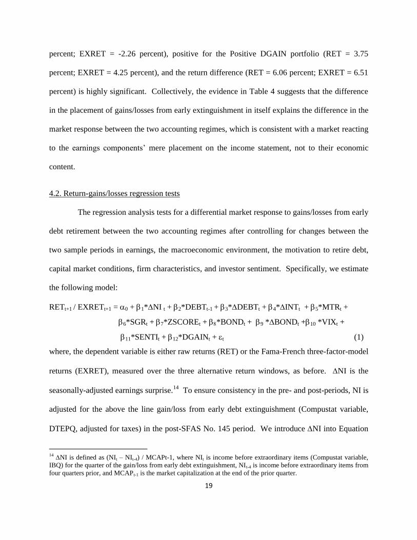
4.2. Return-gains/losses regression tests

The regression analysis tests for a differential market response to gains/losses from early

debt retirement between the two accounting regimes after controlling for changes between the

two sample periods in earnings, the macroeconomic environment, the motivation to retire debt,

capital market conditions, firm characteristics, and investor sentiment. Specifically, we estimate

the following model:

RETt+1 / EXRETt+1 = 0 + 1*NI t + 2*DEBTt-1 + 3*DEBTt + 4*INTt + 5*MTRt +

6*SGRt + 7*ZSCOREt + *BONDt + 9 *BONDt +10 *VIXt +

11*SENTIt + 12*DGAINt + t (1)

where, the dependent variable is either raw returns (RET) or the Fama-French three-factor-model

returns (EXRET), measured over the three alternative return windows, as before. NI is the

seasonally-adjusted earnings surprise.14

To ensure consistency in the pre- and post-periods, NI is

adjusted for the above the line gain/loss from early debt extinguishment (Compustat variable,

DTEPQ, adjusted for taxes) in the post-SFAS No. 145 period. We introduce NI into Equation

14

NI is defined as (NIt – NIt-4) / MCAPt-1, where NIt is income before extraordinary items (Compustat variable,

IBQ) for the quarter of the gain/loss from early debt extinguishment, NIt-4 is income before extraordinary items from

four quarters prior, and MCAPt-1 is the market capitalization at the end of the prior quarter.

20

(1) to control for the earnings surprise released simultaneously with the gain/loss from the early

debt retirement. Based on prior literature, we expect 1 > 0. We exclude NI in the regression

for the 8-K window, as earnings are not yet available at the time of the 8-K release.

Manzon (1994) identifies high-leverage and high-interest burden as motivations to retire

debt early. Hence, we include the level of debt (DEBT), change in debt DEBT), and change in

interest expense (INT) in our regression. Dis lagged total debt scaled by lagged market

capitalization andDEBT is the quarterly change in DEBT. INT is lagged quarterly change in

total interest expense scaled by lagged market capitalization. Manzon (1994) also shows that

firms with higher marginal tax rates are less likely to retire debt, since these firms ascribe a

greater value to the debt tax shield. We thus include MTR, the firm specific marginal tax rate as

estimated by Graham and Mills (2008). In addition, since Manzon (1994) demonstrates that

growing firms are less likely to retire debt, we control for sales growth (SGR), defined as sales

growth rate between current quarterly sales (SALEQ) and quarterly sales from four quarters

prior.15

Since companies in financial distress are less likely to early retire debt, we include

ZSCORE, the Altman Z-Score, in Equation (1).16

BOND is the Moody’s seasoned BAA

15

In untabulated analysis, we replicate Manzon’s analysis (1994) to ensure that the results are prevalent in our

sample and, more importantly, that the motivations behind debt retirements are similar across both the pre- and post-

periods. We estimate a probit model using all quarterly observations on Compustat between 1996 and 2009 with

non-zero long-term debt, using all the variables in Manzon (1994). Consistent with Manzon, the decision to retire

debt is positively associated with leverage and interest burden and negatively associated with sales growth and

marginal tax rate. More importantly, all variables are significant in the expected direction in both periods. A

comparison of the coefficients suggests that the effects of leverage and taxes are marginally stronger in the post-

SFAS No. 145 period.

16 We measure ZSCORE, using Compustat quarterly data, as: 1.2*(WC/ATQ) + 1.4*(REQ/ATQ) +

3.3*(4*OIADPQ/ATQ) + 0.6*(CSHOQ*PRCCQ/LTQ) + 0.999*(4*SALEQ/ATQ). Note that quarterly income

statement data are annualized.

21

corporate bond yield. BOND is the change in BOND compared to the year before.17

We add

these two variables to the regression to control for possible macroeconomic differences (level of

and changes in market interest rate) between our two sample periods. VIX is the Chicago Board

Options Exchange Market Volatility Index, and SENTI is the monthly market sentiment index

obtained from Baker and Wurgler (2007). We introduce these variables to control for possible

changes in capital market conditions or investor behavior between our two sample periods.

DGAIN, our variable of interest, is the after-tax gains or losses from extinguishment of

debt, as defined earlier.18

In terms of Equation (1), the parameter of interest is 12. If the market

responds to gains/losses from early debt extinguishment, we expect 12 > 0.

To address a potential problem of outlying observations that may arise when accounting

data are pooled across firms and over time, we follow the standard approach in the accounting

literature and winsorize all firm-level independent variables at the 1st and 99

th percentiles. In

addition, to control for the effects of firm- and time- clustering, all reported t-statistics are

adjusted for two-way clustering by firm (CUSIP) and time (years), as in Petersen (2009) and

Gow, Ormazabal and Taylor (2010). Finally, we control for industry-fixed effects, using the

Fama and French (1997) industry classification.

Table 5 reports the regression results. In Panel A the dependent variable is raw returns

and in Panel B the Fama-French three-factor-model returns. For each return window, we

estimate Equation (1) in both the pre- and post-SFAS No. 145 periods, and then test for equality

17

We use the yield on BAA bonds because of the risk profile of firms in our sample (smaller and less profitable than

the Compustat universe). Results are nearly identical when we use yield on AAA bonds instead.

18 Firm-specific effective tax rates are estimated as the ratio of quarterly income tax expense (TXTQ) to quarterly

pre-tax income (PIQ). If this information is unavailable, the tax rate is set to the median tax rate across all

observations in the same fiscal year. If the sign of effective tax rate is opposite what would be expected (i.e. income

tax expense despite a pre-tax loss or income tax credit despite a pre-tax profit), tax rate is set to zero. Our variable

DGAIN is set to DTEPQ multiplied by (1 - effective tax rate).

22

between the two corresponding coefficients across the two accounting regimes.19

Before discussing the results for our variable of interest, DGAIN, we note that 1, the

coefficient on our proxy for the quarterly earnings surprise, NI, is significantly positive in the

earnings announcement window in both accounting regimes: 0.082 (t-statistic of 2.57) in the pre-

period and 0.115 (t-statistic = 3.15) in the post-. However, the difference between the two

coefficients, 0.033, is insignificant. The significantly positive coefficient on NI in both sample

periods is consistent with findings in prior literature and thus alleviates concerns that our sample

is not representative. The insignificant difference between the two coefficients across the two

accounting regimes suggests that the market response to earnings news has not materially

changed. We also note that nearly all other control variables are either insignificant or show

insignificant differences across time. This increases our confidence that any differential market

response to gains/losses between the two periods can be attributed to income statement

presentation.

Our variables of interest, DGAIN, has an insignificant coefficient (12) for all three return

windows in the pre-SFAS No. 145. This suggests that investors have not reacted to gains/losses

from early debt extinguishments when they were reported as special item below the line. This is

consistent with Fairfield, Sweeney, and Yohn (1996), who find that special items below the line

have little predictive ability with respect to future earnings.20

It is clear, however, that the market response varies between the two periods for two

reasons. First, in the two return windows around which the gains/losses from early debt

19

For the sake of brevity, the discussion below focuses on the results in Panel A of Table 5; the results in Panel B

are fairly similar, which is not surprising given the short (three-day) return windows. 20

Fairfield, Sweeney, and Yohn (1996) consider special items above and below the line as groups; the components

within each group have not been separately analyzed, however.

23

retirements were announced, the SEC 8-K filings and the earnings announcements, 12 is

significantly positive, 0.141 (t-statistic = 2.41) and 0.086 (t-statistic = 2.16), respectively.

Second, the difference in 12 between the pre- and post-SFAS No. 145 periods in the earnings

announcement window is significantly positive, 0.121 (t-statistic = 1.88).21

Still, the differential

market response may follow from the limited information released on these two return windows,

which does not allow separating earnings to its components. For this alternative story to be

valid, a reversal in 12 should occur in the future, when more information about the gains/losses

becomes publicly available, most likely around the SEC 10Q/10K filing date when the full

financial statements become publicly available. However, inconsistent with this, 12 in this

return window is insignificant (-0.003, t-statistic -0.07) in the pre-SFAS No. 145 period and

significantly positive (0.104, t-statistic 2.98) in the post-SFAS No. 145 period, indicating a

continuation of the response, not a reversal.

Overall, the results from the portfolio return tests in Table 4 and from the return-

gains/losses regression tests in Table 5 suggest that the difference in the placement of

gains/losses from early extinguishment in itself explains the difference in the market response

between the two accounting regimes.

5. Alternative explanations and sensitivity tests

In this section we test alternative explanations that examine changes in: (1) the nature of

extinguishment transactions (cash vs. debt refinancing), (2) the information content of

gains/losses from early retirements, and (3) the market reaction to above and below the line

21

For the SEC 8-K filing window, 11 is significant in the post-SFAS No. 145 period and insignificant in the pre-

period. However, the difference between the two coefficients is insignificant, most likely due to a relatively small

sample size.

24

items. We also perform sensitivity tests that assess the validity of our sample selection

procedure.

5.1. Extinguishment transactions vary across the two accounting regimes

In general, in addition to reacting to the gain/loss from early retirement, the market may

also react to the form in which the retirement is carried out. For example, gains/losses associated

with a plain vanilla extinguishment, financed with cash, may provide little additional

information. Conversely, the market reaction to gains/losses from more complex

extinguishments, such as debt refinancing, may be confounded by its favorable terms. If the

distribution of the nature of extinguishments varies across the two periods, this will affect our

ability to interpret the differential market response.

Recall from Panel D of Table 2 that the two most common forms of funding debt

retirements are through debt refinancing and cash. However, the proportion of debt refinancing

declines from 55.4% to 49.4%, while the proportion of cash based retirements increases from

26.4% to 40.4%. To ensure that this shift does not influence our results, we partition the sample

into cash and debt refinancing subsamples and replicate the regression analysis reported in Table

5.

Panel A and Panel B of Table 6 report, respectively, the results for the debt refinancing

and cash retirement transactions, using the three-day abnormal returns (EXRET) as the

dependent variable. The picture that emerges from comparing the results in Panel A and Panel B

is that the stock returns associated with the gains/losses from cash retirements and debt

refinancing retirements are similar. Consider, for example, the coefficients on DGAIN in the

earnings announcement window. For the subset of debt refinancing retirements (Panel A of

Table 6), in the pre-SFAS No. 145 period the coefficient is close to zero and statistically

25

insignificant (-0.002; t-statistic = -0.02), whereas in the post-SFAS No. 145 it is approximately

eighty times larger (in absolute value) and statistically significant(0.171; t-statistic = 2.70).

Similarly, for the subset of cash retirements (Panel B of Table 6), in the pre-SFAS No. 145

period the coefficient on DGAIN is small and statistically insignificant (-0.044; t-statistic =

-0.50), whereas in the post-SFAS No. 145 it is significantly positive (0.144; t-statistic = 2.57).

Furthermore, in both partitions, the difference between the coefficients across the two accounting

regimes is significant. Overall, the results in Table 6 suggest that the differential reaction to

gains/losses from early retirements across the two accounting regimes cannot be attributed to

differences in the mode of financing across the two regimes.

5.2. Gains/losses from early extinguishment and earnings predictability

Another alternative explanation for our findings is that the future cash flow implications

of the debt retirements differ across the two subperiods. In other words, the observed market

response to the gains/losses from early retirements reflects an improvement in their ability to

predict future firm performance in the post-SFAS No. 145 period. We explore this possibility by

testing the ability of the gains/losses to predict future earnings and cash flows. To that end, we

estimate the following model:

PERFORMANCEt+i = 0 + 1* PERFORMANCE t+ 2*DGAINt +

+ 3*DGAINt*POST + t

where, the dependent variable, PERFORMANCEt+i, is either i-quarter-ahead cash from operation

(CFO) or i-quarter-ahead income before extraordinary items (IBQ). To ensure consistency in the

pre- and post-periods, IBQ is adjusted for the above the line gain from early debt extinguishment

(DTEAQ) in the post-SFAS No. 145 period. The independent variables are PERFORMANCEt,

the performance measure (CFO or IBQ) at the early retirement quarter, and the after tax gain/loss

26

from early debt extinguishment (DGAIN), which is also interacted with a dummy variable

POST that equals 1 for the post-SFAS No. 145 period (after 2002) and 0 otherwise. All

variables are deflated by lagged market value at the beginning of the early debt extinguishment

quarter and, as before, winsorized at the 1st and 99

th percentiles. Also, as before, we include

industry-fixed effects and present two way clustered t-statistics.

In equation (2), if the current performance measure is informative about future

performance, we expect 2 > 0, while if DGAIN is informative about future performance, we

expect 3 > 0. The coefficient of interest, however, is 33. If the ability of DGAIN to predict

future performance has improved between the two accounting regimes, we expect 33 > 0.

Table 7 reports the results from estimating Equation (2), measuring the dependent

variables in quarters t+1 to t+4. In Panel A, the dependent variable is IBQ and in Panel B, the

dependent variable is CFO. Three salient points emerge from these results. First, the coefficient

on current quarterly earnings (1) is significantly positive in all four quarters for both

performance measures. Second, DGAIN generally has little predictive power with respect to

future firm performance. Third, and most important, 33 is never significantly positive for either

performance measure in any of the quarters.22

Thus, the evidence in Table 7 is inconsistent with

an improvement in the predictive ability of DGAIN over time. This increases confidence that the

return pattern we document relates to the position of the gains/losses in the income statement.

5.3. Market reaction to below and above the line items varies across the two accounting regimes

In this section we assess the possibility that investor reaction to below and above the line

22

The only exception is in quarter t+1, when earnings are used as the performance measure. However, in this case

33 is significantly negative, not positive. These results are consistent with Fairfield et al. (2009) who show that

special items generally have an insignificant correlation with future profitability for firms with low profitability (the

majority of this sample) and a negative correlation with future profitability for firms with high profitability.

27

items changed over time, irrespective of the change in the position of gains/losses from early

debt extinguishments in the income statements. To examine this possibility, we compare the

market reaction to gains/losses from special items above the line (Table 8) and from

extraordinary items below the line (Table 9) around earnings announcements and SEC 10Q/10K

filings in the pre- and post-SFAS No. 145 periods. Consider the results in Table 8, focusing on

the earnings announcement widow. In both the pre-period (Panel A) and the post-period (Panel

B), the stock return is negative for the Large Negative portfolio (which contains firms with large

quarterly losses from special items) and positive for the Positive portfolio (containing firms with

quarterly gains from special items). The return difference in both panels is around 2 percent and

is highly significant. The results in Panel C further demonstrate that the market response to

special items has not changed between our two sample periods, as the return difference in

difference between the Positive portfolio and the Large Negative portfolio is insignificant.

Table 9 compares the market reaction to gains/losses from extraordinary items in the pre-

and post-SFAS No. 145 periods. The results in Panel A for the pre-period and in Panel B for the

post-period demonstrate there is no evidence of any market reaction to gains/losses from

extraordinary items. Moreover, the results in Panel C show that formal tests of return difference

in difference between the Positive portfolios and the Large Negative portfolios fail to reject the

null of equality in market response between the two periods. Overall, the results in Table 8 and

Table 9 show no evidence to support the alternative explanations that our results are driven by

differences in how the market reacts to all special items or extraordinary items over time.

5.4. Does our sample selection procedure affect our findings?

Do our results follow from a small number of serial extinguishers? To assess this

possibility, we replicate our tests in Table 4 after partitioning our sample into two approximately

28

equal size subsamples: one containing firms with two or less retirements in both subperiods and

the other more than two retirements in both subperiods.

The results displayed in Table 10 clearly demonstrate that the differential market

response to early retirements between the two accounting regimes is observed in both

subsamples, and that the results for the two subsamples are fairly similar to the results for the

entire sample, reported in Table 4. Specifically, focusing on the earnings announcement window

and the SEC 10Q/10K filing window, the results in Panel A of Table 7 show no stock price

response to gains/losses from early retirements in the pre-SFAS No. 145 period, but significant

response in the post-period. Likewise, the results in Panel B for the “serial extinguishers” show

no stock price response in the pre-period and significant response in the post-period (albeit only

marginally significant in the earnings announcement window).23

Overall, the results in Table 10

show that the differential stock price response across the two accounting regimes relates to all

extinguishers, not only to a small subset of them.

Finally, we examine the possibility that our findings are not generalizable because our

sample selection results in a biased sample. As discussed earlier, we impose restrictions on our

sample to increase statistical power (the gain/loss must be material) and to alleviate concerns that

alternative explanations underlie our findings (a firm must early retire in both accounting

regimes). Such an approach, however, may cast doubt on the generalizability of our finding. To

assess this possibility, we analyze the market response to gains/losses from early retirements

after removing the first sample-selection restriction (Table 11) and then both restrictions (Table

23

Interestingly, the stock-price response in the subsample of frequent extinguishers is about half of that of the

infrequent extinguishers. For example, around earnings announcements EXRET, the Fama-French three-factor-

model return is 8.59 percent for the latter and only 5.07 percent for the former. This may be expected, as investors

are likely able to better anticipate and therefore are less surprised by the gains/losses from early extinguishments in

firms that engage in such transactions regularly.

29

12).

We first relax the restriction that that the after-tax gain/loss be greater in absolute

magnitude than one percent of quarterly sales. Our sample here consists of all firms with

extraordinary items (Compustat item XIQ) in the pre-SFAS No. 145 period that also had

reported gains/losses from debt extinguishment (Compustat item DTEPQ) in the post-SFAS No.

145 period.24

The results reported in Table 11 show that removing the first restriction has little

effect on our finding. Specifically, the results in Panel A show no market response to

gains/losses from early retirements in the pre-SFAS No. 145 and the results in Panel B show a

significant market response in the post-period. Moreover, the difference in differences between

the returns to the Positive portfolios and the Large Negative portfolios reported in Panel C

continue to be significant. Next, we further relax the restriction that a given firm needs to have

at least one observation in the two subperiods. The results, presented in Table 12, are

qualitatively similar to those in Table 11, showing that our finding is robust to both sample

selection criteria.

6. Conclusion

Does the placement in the income statement in itself relate to the market response of an

earnings component? We investigate this question by exploiting a recent change in the reporting

requirements for gains/losses from early debt extinguishment. SFAS No. 145, which became

effective after May 15, 2002, rescinded SFAS No. 4 that required material gains and losses from

early extinguishment of debt be classified as extraordinary items below the line. As a result, in

24

The sample size for this sensitivity test is significantly bigger than the sample used for our primary tests. Given

the large sample size, we are unable to conduct the verification procedure to ensure that all the observations

correspond to debt retirements and rely on prior evidence that suggests that a vast preponderance of extraordinary

items in the pre-SFAS No.1 45 period did correspond to debt retirements.

30

the post SFAS No. 145 period, these gains and losses are classified as extraordinary items only if

they meet the criteria in APB No. 30: they are caused by an event that is both unusual and

infrequent. Since extinguishment of debt rarely meets these dual criteria, the related gains/losses

are reported above the line in the post-SFAS No. 145 period. This reporting change allows us to

test our research question.

We analyze a sample that spans both the pre-SFAS No. 145 period from 1996 to mid-

2002 (258 observations), and the post-SFAS No. 145 period from mid-2002 to 2009 (342

observations). We perform both portfolio return tests and return-gains/losses regression tests

that assess the market response to gains/losses from early debt extinguishment in 3-day return

windows around SEC 8-K filing, earnings announcement, and SEC 10Q/10K filing.

Our primary finding is that the market response to gains/losses from early debt

extinguishment varies significantly between the two accounting regimes. In the pre-SFAS No.

145 period, results from portfolio return tests show no market response in any of the three return-

windows examined. Conversely, in the post-SFAS No. 145 period, the portfolio tests show a

significant market response to gains/losses from early extinguishment in both the earnings

announcement window and the SEC 10Q/10K filing window. A differences-in-differences test

shows a significant shift in market response between the two accounting regimes. Results from

the return-gains/losses regression analysis that considers a variety of control variables for firm

characteristics, the motivation to early retire debt, the macroeconomic environment, the capital

market condition, and investor behavior confirm our portfolio return test result that in the post-

period, the market reacts to the same gains/losses that it was ignoring in the pre-period.

Moreover, examination of alternative explanations and sensitivity tests demonstrate that our

results are robust. This suggests that the change in the position within the income statement of

31

the gains/losses in itself explains the differential market response.

We contribute to the literature on the importance of income statement presentation by

being the first to demonstrate that the placement of a line item on the income statement in itself

has important valuation implications. This seems particularly timely and important in light of

the recent Proposed Accounting Standards Update on Financial Statement Presentation issued by

FASB. In addition, this finding complements prior results indicating that managers

opportunistically engage in expense classification shifting (e.g., McVay 2006; Barua 2010) out

of a desire for a higher stock price.

32

References

Ball, R., Brown, P., 1968. An empirical evaluation of accounting income numbers. Journal of

Accounting Research 6, 159 – 177.

Bartov, E., Balakrishnan, K., Faurel, L., 2010. Post Loss/Profit Announcement Drift. Journal of

Accounting and Economics 50, 20 - 41.

Bartov, E., Bodnar, G.M., 1994. Firm Valuation, Earnings Expectations, and the Exchange-Rate

Exposure Effect. The Journal of Finance 49, 1755 - 1785.

Bartov, E., Mohanram, P., 2004. Private Information, Earnings Manipulations, and Executive

Stock Option Exercises. The Accounting Review 79, 889 – 920.

Barua, A., Lin, S., and Sbaraglia, A. M., 2010. Earnings Management Using Discontinued

Operations. The Accounting Review 85, 1485 - 1509.

Beaver, W., 1968. The information content of annual earnings announcements. Journal of

Accounting Research Supplement 6, 67 – 92.

Bradshaw, M., Sloan, R., 2002. GAAP versus The Street: An Empirical Assessment of Two

Alternative Definitions of Earnings. Journal of Accounting Research 40, 41 - 66.

Burgstahler, D., Jiambalvo, J., Shevlin, T., 2002. Do Stock Prices Fully Reflect the Implications

of Special Items for Future Earnings? Journal of Accounting Research 40, 585 - 612

Davis-Friday, P., Folami, L., Liu, C., Mittelstaedt, H., 1999. The Value Relevance of Financial

Statement Recognition vs. Disclosure: Evidence from SFAS No. 106. The Accounting

Review 74, 403 - 423.

Elliott, J., Hanna, J., 1996. Repeated Accounting Writeoffs and the Information Content of

Earnings. Journal of Accounting Research 34 (supplement), 135-155.

Espahbodi, H., Espahbodi, P., Rezaee, Z., and Tehranina, H., 2002. Stock Price Reaction and

Value Relevance of Recognition versus Disclosure: The Case of Stock-Based

Compensation. Journal of Accounting and Economics 33, 343 - 373.

Fairfield, P, Kitching, K., and Tang, V., 2009. Are special items informative about future profit

margins? Review of Accounting Studies 14, 204-236.

Fairfield, P, Sweeney, R., Yohn, T., 1996. Accounting Classification and the Predictive Content

of Earnings. The Accounting Review 71, 337 - 355.

Fama, E., French. K. 1997. Industry Costs of Equity. Journal of Financial Economics 43, 153 -

193.

33

Gow, I., Ormazabal, G., Taylor, D., 2010. Correcting for Cross-Sectional and Time-Series

Dependence in Accounting Research. The Accounting Review 85, 483 - 512.

Graham, J.R, Mills, L. , 2008. Simulating Marginal Tax Rates Using Tax Return Data, Journal

of Accounting and Economics 46, 366-388.

Hand, J., 1989. Did Firms Undertake Debt-Equity Swaps for an Accounting Paper Profit or True

Financial Gain? The Accounting Review 64, 587 - 623.

Hand, J., 1990. A test of the extended functional fixation hypothesis. The Accounting Review 65,

740 - 763.

Hirst, D.E., Hopkins, P.E., 1998. Comprehensive Income Reporting and Analysts’ Valuation

Judgments. Journal of Accounting Research 36 Supplement, 47 – 75.

Lipe, R., 1986. The information contained in the components of earnings. Journal of Accounting

Research 24, 37–64.

Luft, J. L., Shields, M.D, 2001. Why Does Fixation Persist? Experimental Evidence on the

Judgment of Performance Effects of Expensing Intangibles. The Accounting Review

76(4), 561-588.

Maines, L.A., McDaniel, L.S., 2000. Effects of Comprehensive-Income Characteristics on

Nonprofessional Investors' Judgments: The Role of Financial-Statement Presentation

Format. The Accounting Review 75, 179-207.

Manzon, G.B., 1994. The Role of Taxes in Early Debt Retirement. Journal of the American Tax

Association 16, 87-100.

McVay, S., 2006. Earnings Management Using Classification Shifting. The Accounting Review

81, 501 - 531.

Ohlson, J., Penman, S., 1992. Disaggregated Accounting Data as Explanatory Variables for

Returns. Journal of Accounting, Auditing and Finance 7, 553 – 573.

Petersen. M., 2009. Estimating Standard Errors in Finance Panel Data Sets: Comparing

Approaches. Review of Financial Studies 22, 435-480.

Riedl, E., Srinivasan, S., 2010. Signaling Firm Performance through Financial Statement

Presentation: An Analysis using Special Items. Contemporary Accounting Research 27,

289-332.

Securities and Exchange Commission, Letter: 2000 Audit Risk Alert to the American Institute of

Certified Public Accountants (Washington, D.C.: Securities and Exchange Commission,

October 13, 2000).

34

Simko, P.J., 1999. Financial Instrument Fair Values and Nonfinancial Firms. Journal of

Accounting, Auditing and Finance 14(3), pp. 247 – 274.

Sougiannis, T., Chambers, D., Linsmeier, T., Shakespeare, C., 2007. An Evaluation of SFAS

No. 130 Comprehensive Income Disclosures. Review of Accounting Studies 12, 557 –

593.

Strong. N., Walker, M., 1993. The Explanatory Power of Earnings for Stock Returns. The

Accounting Review 68, 385-399.

35

APPENDIX I

Income Statement Disclosure of Gains/Losses from Early Debt Extinguishment

before and after SFAS No. 145

Pre-SFAS No. 145 Example

ARGOSY GAMING COMPANY CONDENSED CONSOLIDATED STATEMENTS OF INCOME

(In Thousands, Except Share and Per Share Data)

SEPTEMBER

30,

SEPTEMBER

30,

1999 1998

(UNAUDITED) (UNAUDITED)

REVENUES:

Casino $147,267 $124,330

Admissions 5,057 4,581

Food, beverage and other 15,265 13,780

167,589 142,691

Less promotional allowances -11,020 -9,158

Net revenues 156,569 133,533

COSTS AND EXPENSES:

Casino 65,610 57,935

Food, beverage and other 10,612 10,473

Other operating expenses 7,113 6,847

Selling, general and administrative 30,053 24,129

Depreciation and amortization 8,628 8,452

122,016 107,836

Income from operations 34,553 25,697

OTHER INCOME (EXPENSE):

Interest income 684 933

Interest expense -10,732 -14,627

-10,048 -13,694

Income before minority interests, income taxes 24,505 12,003

Minority interests -9,587 -7,697

Income tax expense -600 -195

Net income before extraordinary item 14,318 4,111

Extraordinary loss on extinguishment of debt -3,660

NET INCOME 10,658 4,111

36

APPENDIX I (Cont’d)

Income Statement Disclosure of Gains/Losses from Early Debt Extinguishment

before and after SFAS No. 145

Post-SFAS No. 145 Example

ARGOSY GAMING COMPANY CONDENSED CONSOLIDATED STATEMENTS OF INCOME

(In Thousands, Except Share and Per Share Data)

Three Months Ended

March 31,

2004 2003

(unaudited) (unaudited)

Revenues:

Casino $ 266,007 $ 240,857

Admissions 5,360 3,005

Food, beverage and other 26,460 24,760

297,827 268,622

Less promotional allowances (33,738 ) (32,290 )

Net revenues 264,089 236,332

Costs and expenses:

Gaming and admission taxes 91,578 79,857

Casino 32,574 34,146

Selling, general and administrative 44,176 35,789

Food, beverage and other 18,601 17,798

Other operating expenses 9,863 10,506

Depreciation and amortization 14,225 12,683

211,017 190,779

Income from operations 53,072 45,553

Other income (expense):

Interest income 21 51

Interest expense (18,051 ) (18,947 )

Expense on early retirement of debt (25,277 ) —

(43,307 ) (18,896 )

Income before income taxes 9,765 26,657

Income tax expense (5,805 ) (11,996 )

Net income $ 3,960 $ 14,661

37

Appendix II

Variable Definitions for Regression Analysis

Variable Definition

NI

Seasonally-adjusted earnings surprise.

DEBTt-1

Lagged total debt (sum of short term debt DLCQ and long term debt DLTTQ) scaled by lagged

market capitalization (PRCCQ * CSHO).

DEBTt Change in total debt scaled by lagged market capitalization

INTt Change in total interest expense scaled by lagged market capitalization.

MTR Firm specific marginal tax rate obtained from Graham and Mills (2008)

SGR Sales growth between current sales (SALEQ) and sales from 4 quarters prior.

ZSCORE

Altman Z-Score, computed at the end of the quarter of debt extinguishment

BOND

Moody’s seasoned BAA corporate bond yield

BOND

Change in BOND compared to one year before

VIX

Chicago Board Options Exchange Market Volatility Index.

SENTI

Monthly market sentiment index obtained from Baker and Wurgler (2007).

DGAIN

The after tax gains or losses from extinguishment of debt. For pre-FAS145 period, DGAIN is

hand-collected from 10-Q or 10-K. For the post-145 period, DGAIN is equal to the pre-tax gain

or loss from debt retirement (DTEPQ) from the Compustat FUNDQ database, adjusted for

taxes using the firm specific tax rate. DGAIN is deflated by lagged market value. NI the

seasonally-adjusted earnings surprise.

38

Table 1

Sample Composition

Criterion

# of Obs.

Pre-SFAS

No. 145

# of Obs.

Post-SFAS

No. 145

# of Distinct

Firms

Observations from 1996 to 2009 with required financial data on

Compustat and returns data on CRSP

3207 4269 2834

Firms incorporated in US 2899 3984 2571

Subset that is not in financial services (SIC 6000 -7000)

2340 3121 2091

Gain/loss from early extinguishment is at least one percent of quarterly

sales

1639 1824 1779

Firms with at least one observation pre-FAS 145 and post-FAS 145

552 739 308

Removal of observations verified as extraordinary items unrelated to

early debt extinguishment (pre-FAS 145) (and corresponding removal

of observations post-FAS 145 without any pre-FAS 145 observations

for a given firm)

380 495 200

FINAL CLEAN UP STEPS

Removal of observations where line item disclosure is not

explicitly provided on the income statement in the post-FAS

145 period (124 observations)

Removal of observations where extraordinary item

description in the pre-FAS 145 period does not explicitly

mention debt retirement (103 observations)

Deletion of Troubled Debt Restructurings

(8 in the pre-period and 2 in the post-period)

Ensuring that matching maintained in the pre and post period

FINAL SAMPLE 258 342 135

39

Table 2

Sample Distribution

Panel A: Industry Distribution using the Fama and French (1997) Classification

Pre-FAS 145 Post-FAS 145

FF Group Description N Proportion (%) N Proportion (%)

1 Agriculture 2 0.8% 2 0.6% 2 Food Products 2 0.8% 2 0.6% 4 Beer & Liquor 0 0.0% 1 0.3% 5 Tobacco Products 0 0.0% 4 1.2% 6 Recreation 1 0.4% 3 0.9% 7 Entertainment 15 5.8% 21 6.1% 8 Printing And Publishing 1 0.4% 4 1.2% 9 Consumer Goods 5 1.9% 6 1.8% 11 Healthcare 12 4.7% 14 4.1% 12 Medical Equipment 1 0.4% 1 0.3% 13 Pharmaceutical Products 10 3.9% 19 5.6% 14 Chemicals 7 2.7% 14 4.1% 15 Rubber And Plastic Products 2 0.8% 2 0.6% 16 Textiles 1 0.4% 3 0.9% 18 Construction 6 2.3% 4 1.2% 19 Steel Works 1 0.4% 1 0.3% 20 Fabricated Products 1 0.4% 1 0.3% 21 Machinery 6 2.3% 4 1.2% 22 Electrical Equipment 3 1.2% 5 1.5% 23 Automobiles And Trucks 2 0.8% 2 0.6% 26 Defense 4 1.6% 1 0.3% 27 Precious Metals 5 1.9% 9 2.6% 28 Non Metallic Mining 1 0.4% 0 0.0% 29 Coal 1 0.4% 1 0.3% 30 Petroleum And Natural Gas 36 14.0% 18 5.3% 31 Utilities 5 1.9% 3 0.9% 32 Communications 42 16.3% 97 28.4% 33 Personal Services 4 1.6% 8 2.3% 34 Business Services 12 4.7% 29 8.5% 35 Computers 6 2.3% 2 0.6% 36 Electronic Equipment 15 5.8% 21 6.1% 37 Measuring And Control Eqp. 3 1.2% 1 0.3% 38 Business Supplies 4 1.6% 8 2.3% 39 Shipping Containers 2 0.8% 2 0.6% 40 Transportation 13 5.0% 6 1.8% 41 Wholesale 4 1.6% 6 1.8% 42 Retail 7 2.7% 6 1.8% 43 Restaurants, Hotels & Motels 7 2.7% 3 0.9% 48 Other 9 3.5% 8 2.3%

Total 258 100.0 342 100.0

40

Table 2 (Cont’d)

Sample Distribution

Panel B: Time Distribution

Pre-SFAS 145 Period Post-SFAS 145 Period

Year N Proportion (%) Year N Proportion (%)

1996 18 7.0 2002 21 6.1

1997 40 15.5 2003 70 20.5

1998 42 16.3 2004 75 21.9

1999 30 11.6 2005 56 16.4

2000 47 18.2 2006 36 10.5

2001 53 20.5 2007 27 7.9

2002 28 10.9 2008 17 5.0

2009 40 11.7

TOTAL 258 TOTAL 342

Panel C: Fiscal Quarter Distribution

Pre-SFAS No. 145 Period Post-SFAS No. 145 Period

Quarter N Proportion (%) Quarter N Proportion (%)

1 51 19.8 1 86 25.1

2 76 29.5 2 91 26.6

3 67 26.0 3 68 19.9

4 64 24.8 4 97 28.4

TOTAL 258

342

Panel D: Funding of Debt Retirement Distribution

Pre-SFAS No. 145 Period Post-SFAS No. 145 Period

Funding N Proportion (%) Funding N Proportion (%)

Cash 68 26.4 Cash 138 40.4

Debt 143 55.4 Debt 169 49.4

Equity 25 9.7 Equity 13 3.8

Hybrid 22 8.5 Hybrid 22 6.4

TOTAL 258

342

Panel E: 8-K Filing of Debt Retirement Distribution

Pre-SFAS No. 145 Period Post-SFAS No. 145 Period

Disclosure N Proportion (%) Disclosure N Proportion (%)

8-K 102 39.5% 8-K 115 33.6%

No 8-K 156 60.5% No 8-K 227 66.4%

TOTAL 258

342

41

Table 3

Sample Descriptive Statistics

DGAIN is after tax gains or losses from extinguishment of debt. For pre-FAS145 period, DGAIN is hand-collected from 10-Q or

10-K. For the post-145 period, DGAIN is equal to the pre-tax gain or loss from debt retirement (DTEPQ) from the Compustat

FUNDQ database, adjusted for taxes using the firm-specific tax rate. ATQ is total assets. MCAP is market capitalization defined

as ending stock price (PRCCQ) times shares outstanding (CSHOQ) from the prior quarter. IBQ is quarterly income before

extraordinary items. DEBT is the sum of short term debt (DLCQ) and long term debt (DLTTQ) scaled by market capitalization.

DEBT is the change in total debt with respect to the prior quarter, also scaled by market capitalization. INT is change in

interest expense with respect to the previous quarter, scaled by market capitalization. NI is the change in income before

extraordinary items with respect to the previous quarter, scaled by market capitalization. Panel B presents raw returns (RET) and

Fama-French 3 factor adjusted excess returns (EXRET) computed in the three day window around 8-K release, earnings

announcement and SEC filing. Panel C compares sample firm characteristics with the universe of firms on Compustat (excluding

SIC 6000-7000). T-statistics for differences are calculated using a pooled estimate of standard error using the Satterthwaite

method. Z-statistics for differences in medians are from Wilcoxon sign-rank tests. Significance levels for difference are

represented by*** (1%), **

(5%) and * (10%).

Panel A: Firm Characteristics

Variable Mean

Pre-145

Mean

Post-145

Diff

(Post-Pre) t-stat

Median

Pre-145

Median

Post-145

Diff

(Post-Pre) z-stat

% DGAINt > 0 27.5% 21.1% -6.5% -1.82* 0.0% 0.0% 0.0% -1.83*

DGAINt -1.26 -3.53 -2.27 -0.24 -3.22 -5.87 -2.65 -2.86***

|DGAINt| 21.46 20.98 -0.48 -0.05 4.92 7.95 3.03 4.26***

DGAINt/MCAPt-1 0.8% 2.4% 1.7% 1.39 -0.4% -0.6% -0.2% -2.21***

|DGAINt/MCAPt-1| 4.6% 10.7% 6.1% 1.98** 1.1% 1.2% 0.1% 1.58

|DGAINt|/|IBQt| 1.57 2.25 0.68 1.82* 0.58 0.59 0.01 0.03

IBQt -9.19 5.23 14.42 1.40 0.79 0.73 -0.06 -0.57

LOSS 45.7% 48.0% 2.2% 0.54 0.0% 0.0% 0.0% 0.53

SALEQt 317 289 -28 -0.48 116 166 50 2.55***

ATQt-1 2731 2313 -418 -0.81 941 1247 307 2.27**

MCAPt-1 1907 1485 -422 -1.11 609 650 41 0.80

DEBTt-1 123.3% 193.7% 70.4% 3.50*** 70.0% 77.6% 7.7% 1.30

DEBTt 4.0% -4.8% -8.8% -2.95*** 0.0% -1.3% -1.3% -2.60***

INTt 0.05% -0.11% -0.15% -1.86* 0.00% -0.03% -0.03% -3.64***

NIt -0.88% -0.20% 0.68% 0.44 -0.06% 0.27% 0.33% 2.36**

Panel B: Stock returns (%)

Window Return Mean

Pre-145

Mean

Post-145

Diff

(Post-Pre) t-stat

Median

Pre-145

Median

Post-145

Diff

(Post-Pre)

z-stat

8-K

Release RET 0.24 -0.01 -0.25 -0.24 0.18 -0.17 -0.35 -0.05 EXRET 0.53 -0.09 -0.63 -0.66 -0.08 -0.28 -0.20 -0.11

Earnings

Annc RET 0.30 0.19 -0.11 -0.13 0.00 0.00 0.00 -0.53 EXRET 0.25 0.19 -0.06 -0.07 -0.21 0.25 0.46 0.52

SEC

Filing RET 0.39 -0.26 -0.65 -0.90 0.00 -0.55 -0.55 1.02 EXRET 0.18 -0.02 -0.21 -0.29 -0.28 -0.18 0.10 0.02

42

Table 3 (Cont’d)

Sample Descriptive Statistics

Panel C: Mean Firm Characteristics compared to Compustat universe

Variable Sample

Pre-145

All Firms

Pre-145

Diff

(Sample-

All Firms)

t-stat Sample

Post-145

All Firms

Post-145

Diff

(Sample-

All Firms)

t-stat

IBQt -9.19 15.30 -24.49 -5.20*** 5.23 35.05 -29.82 -3.51***

LOSS 45.7% 45.2% 0.50% 0.55 48.0% 49.8% -1.80% -2.28**

SALEQt 317 354 -37 -0.95 289 627 -338 -5.92***

ATQt-1 2731 2883 -152 -0.34 2313 7512 -5199 -4.28***

MCAPt-1 1907 1546 361 1.68* 1485 2418 -933 -4.21***

DEBTt-1 123.3% 39.3% 84.00% 37.29*** 193.7% 42.6% 151.10% 71.27***

Panel D: Median Firm Characteristics compared to Compustat universe

Variable Sample

Pre-145

All Firms

Pre-145

Diff

(Sample-

All Firms)

t-stat Sample

Post-145

All Firms

Post-145

Diff

(Sample-

All Firms)

t-stat

IBQt 1.38 0.37 1.01 1.47 -2.11 0.52 -2.64 -2.06**

SALEQt 103 19 84.06 11.58*** 159 27 132.75 13.35***

ATQt-1 711 123 587.66 12.13*** 1130 229 900.58 13.46***

MCAPt-1 568 89 478.75 11.13*** 640 143 496.72 11.75***

DEBTt-1 66.0% 0.7% 65.4% 16.70*** 84.7% 1.6% 83.0% 23.06***

Panel E: Mean Firm Characteristics partitioned on whether firms disclose 8-Ks or not

Variable No 8-K

Pre-145

8-K

Pre-145

Diff

t-stat No 8-K

Post-145

8-K

Post-145

Diff

t-stat

% DGAINt > 0 35.9% 14.7% -21.2% -4.06*** 25.1% 13.0% -12.1% -2.82***

DGAINt -4.49 3.67 8.16 0.46 0.77 -12.03 -12.80 -1.30

|DGAINt| 14.35 32.34 17.99 1.02 22.72 17.56 -5.16 -0.54

DGAINt/MCAPt-1 0.8% 0.7% -0.1% -0.09 3.4% 0.4% -3.0% -1.65

|DGAINt/MCAPt-1| 3.6% 6.1% 2.4% 0.76 11.3% 9.3% -2.0% -0.34

|DGAINt|/|IBQt| 1.54 1.61 0.07 0.17 2.52 1.73 -0.79 -1.30

IBQt -11.80 -5.21 6.59 0.36 -1.55 18.61 20.17 1.49

LOSS 47.4% 43.1% -4.3% -0.68 48.0% 47.8% -0.2% -0.03

SALEQt 305 335 30 0.27 280 305 25 0.46

ATQt-1 2644 2864 220 0.22 2240 2458 218 0.56

MCAPt-1 2021 1733 -288 -0.46 1276 1898 621 1.76*

DEBTt-1 132.3% 109.6% -22.7% -1.16 200.9% 179.6% -21.3% -0.61

DEBTt 0.2% 9.7% 9.5% 1.94* -6.4% -1.7% 4.7% 1.25

INTt 0.02% 0.09% 0.08% 0.65 -0.20% 0.07% 0.26% 2.16**

NIt -0.34% -1.72% -1.38% -0.63 -0.80% 0.97% 1.77% 0.92

43

Table 4

Portfolio analyses: Tests for market response around early debt retirements

The analysis variable is either raw returns (RET) or Fama-French 3 factor adjusted excess returns (EXRET) computed in the three day window around 8-K release, earnings announcement and

SEC filing. DGAIN is after tax gains or losses from extinguishment of debt. For pre-FAS145 period, DGAIN is hand-collected from 10-Q or 10-K. For the post-145 period, DGAIN is equal to

the pre-tax gain or loss from debt retirement (DTEPQ) from the Compustat FUNDQ database, adjusted for taxes using the firm specific tax rate. DGAIN is deflated by lagged market value. NI

the seasonally-adjusted earnings surprise. In each year, all observations are divided into three groups. Firms with negative DGAIN are split into two groups (Large Negative and Small Negative),

while firms with positive DGAIN are analyzed separately. Figures in parentheses represent t-statistics for the difference using the Satterthwaite method. Significance levels for difference are

represented by*** (1%), **

(5%) and * (10%).

Panel A: Pre-SFAS No. 145 Period

Returns around

SEC 8-K Filings Returns around

Earnings Announcements Returns around

SEC 10Q/10K Filings DGAIN

Portfolios N Mean

DGAIN (%) Mean

NIt (%) N RET EXRET N RET EXRET N RET EXRET

Large Negative 93 -4.04% -3.42% 47 0.73% 0.79% 93 0.05% 0.00% 93 0.23% 0.20%

Small Negative 94 -0.39% -1.45% 40 0.00% 0.33% 94 1.22% 1.27% 94 0.15% -0.20%

Positive 71 10.89% 3.74% 15 -0.63% 0.28% 71 -0.59% -0.77% 71 0.93% 0.66%

Positive – Large Negative 14.93% 7.16% -1.36% -0.51% -0.63% -0.77% 0.70% 0.46%

t-statistics NA (1.04) (-0.44) (-0.19) (-0.41) (-0.52) (0.56) (0.37)

Panel B: Post-SFAS No. 145 Period Returns around

SEC 8-K Filings Returns around

Earnings Announcements Returns around

SEC 10Q/10K filings DGAIN

Portfolios N Mean

DGAIN (%) Mean

NIt (%) N RET EXRET N RET EXRET N RET EXRET

Large Negative 135 -9.46% -0.55% 51 -0.36% -0.68% 135 -2.01% -1.82% 135 -2.31% -2.26%

Small Negative 135 -0.48% 0.47% 49 -0.62% 0.14% 135 0.68% 0.73% 135 -0.35% -0.06%

Positive 72 31.97% 4.10% 15 3.19% 1.12% 72 3.38% 2.95% 72 3.75% 4.25%

Positive – Large Negative 41.43% 4.65% 3.55% 1.80% 5.39% 4.77% 6.06% 6.51%

t-statistics NA (0.59) (0.85) (0.46) (2.15) ** (1.93) * (2.63) *** (2.94) ***

Panel C: Differences in differences in returns between Positive and Large Negative DGAIN firms (Post – Pre) -2.51% 4.91% 2.31% 6.02% 5.54% 5.36% 6.05% (-0.24) (0.94) (0.49) (2.05) ** (1.92) * (2.04) ** (2.38) **

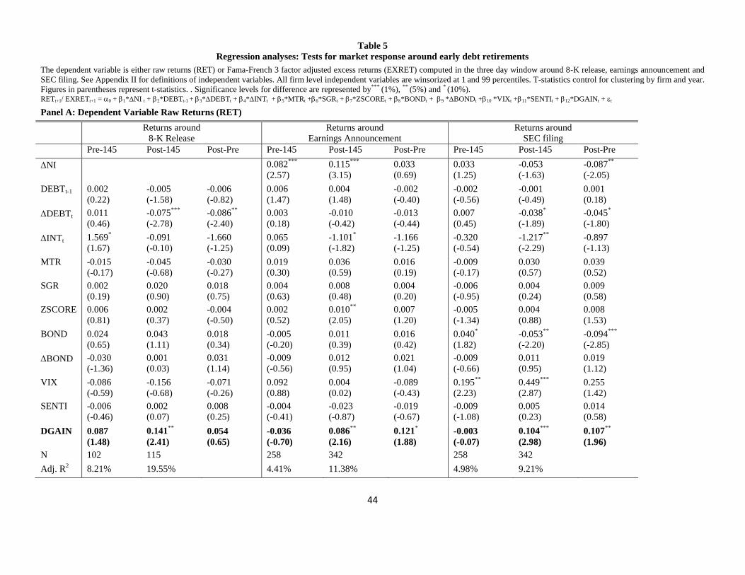
44

Table 5

Regression analyses: Tests for market response around early debt retirements

The dependent variable is either raw returns (RET) or Fama-French 3 factor adjusted excess returns (EXRET) computed in the three day window around 8-K release, earnings announcement and

SEC filing. See Appendix II for definitions of independent variables. All firm level independent variables are winsorized at 1 and 99 percentiles. T-statistics control for clustering by firm and year.

Figures in parentheses represent t-statistics. . Significance levels for difference are represented by*** (1%), **

(5%) and * (10%). RETt+1/ EXRETt+1 = 0 + 1*NI t + 2*DEBTt-1 + 3*DEBTt + 4*INTt + 5*MTRt +6*SGRt + 7*ZSCOREt + *BONDt + 9 *BONDt +10 *VIXt +11*SENTIt + 12*DGAINt + t

Panel A: Dependent Variable Raw Returns (RET)

Returns around

8-K Release

Returns around

Earnings Announcement

Returns around

SEC filing

Pre-145 Post-145 Post-Pre Pre-145 Post-145 Post-Pre Pre-145 Post-145 Post-Pre

NI

0.082***

(2.57)

0.115***

(3.15)

0.033

(0.69)

0.033

(1.25)

-0.053

(-1.63)

-0.087**

(-2.05)

DEBTt-1

0.002

(0.22)

-0.005

(-1.58)

-0.006

(-0.82)

0.006

(1.47)

0.004

(1.48)

-0.002

(-0.40)

-0.002

(-0.56)

-0.001

(-0.49)

0.001

(0.18)

DEBTt

0.011

(0.46)

-0.075***

(-2.78)

-0.086**

(-2.40)

0.003

(0.18)

-0.010

(-0.42)

-0.013

(-0.44)

0.007

(0.45)

-0.038*

(-1.89)

-0.045*

(-1.80)

INTt

1.569*

(1.67)

-0.091

(-0.10)

-1.660

(-1.25)

0.065

(0.09)

-1.101*

(-1.82)

-1.166

(-1.25)

-0.320

(-0.54)

-1.217**

(-2.29)

-0.897

(-1.13)

MTR

-0.015

(-0.17)

-0.045

(-0.68)

-0.030

(-0.27)

0.019

(0.30)

0.036

(0.59)

0.016

(0.19)

-0.009

(-0.17)

0.030

(0.57)

0.039

(0.52)

SGR

0.002

(0.19)

0.020

(0.90)

0.018

(0.75)

0.004

(0.63)

0.008

(0.48)

0.004

(0.20)

-0.006

(-0.95)

0.004

(0.24)

0.009

(0.58)

ZSCORE

0.006

(0.81)

0.002

(0.37)

-0.004

(-0.50)

0.002

(0.52)

0.010**

(2.05)

0.007

(1.20)

-0.005

(-1.34)

0.004

(0.88)

0.008

(1.53)

BOND

0.024

(0.65)

0.043

(1.11)

0.018

(0.34)

-0.005

(-0.20)

0.011

(0.39)

0.016

(0.42)

0.040*

(1.82)

-0.053**

(-2.20)

-0.094***

(-2.85)

BOND

-0.030

(-1.36)

0.001

(0.03)

0.031

(1.14)

-0.009

(-0.56)

0.012

(0.95)

0.021

(1.04)

-0.009

(-0.66)

0.011

(0.95)

0.019

(1.12)

VIX

-0.086

(-0.59)

-0.156

(-0.68)

-0.071

(-0.26)

0.092

(0.88)

0.004

(0.02)

-0.089

(-0.43)

0.195**

(2.23)

0.449***

(2.87)

0.255

(1.42)

SENTI

-0.006

(-0.46)

0.002

(0.07)

0.008

(0.25)

-0.004

(-0.41)

-0.023

(-0.87)

-0.019

(-0.67)

-0.009

(-1.08)

0.005

(0.23)

0.014

(0.58)

DGAIN

0.087

(1.48)

0.141**

(2.41)

0.054

(0.65)

-0.036

(-0.70)

0.086**

(2.16)

0.121*

(1.88)

-0.003

(-0.07)

0.104***

(2.98)

0.107**

(1.96)

N 102 115 258 342 258 342

Adj. R2 8.21% 19.55% 4.41% 11.38% 4.98% 9.21%

45

Table 5 (Cont’d)

Regression analyses: Tests for market response around early debt retirements

Panel B: Dependent Variable 3-factor adjusted Excess Returns (EXRET)

Returns around

8-K Release

Returns around

Earnings Announcement

Returns around

SEC filing

Pre-145 Post-145 Post-Pre Pre-145 Post-145 Post-Pre Pre-145 Post-145 Post-Pre

NI

0.094***

(3.07)

0.118***

(3.32)

0.025

(0.53)

0.037

(1.38)

-0.041

(-1.33)

-0.078*

(-1.91)

DEBTt-1

0.002

(0.29)

-0.006*

(-2.26)

-0.008

(-1.14)

0.007*

(1.78)

0.004

(1.50)

-0.003

(-0.62)

-0.002

(-0.62)

-0.001

(-0.59)

0.001

(0.19)

DEBTt

0.014

(0.65)

-0.08***

(-3.24)

-0.094***

(-2.87)

0.002

(0.14)

-0.004

(-0.16)

-0.006

(-0.22)

0.009

(0.60)

-0.034*

(-1.74)

-0.043*

(-1.75)

INTt

1.399

(1.62)

-0.54

(-0.63)

-1.939

(-1.60)

0.135

(0.20)

-1.121*

(-1.89)

-1.257

(-1.40)

-0.479

(-0.80)

-1.260**

(-2.46)

-0.780

(-0.99)

MTR

-0.013

(-0.16)

-0.013

(-0.21)

0.00

(0.00)

0.035

(0.58)

0.034

(0.57)

-0.001

(-0.02)

-0.012

(-0.22)

0.031

(0.61)

0.043

(0.58)

SGR

0.000 (0.01)

0.028 (1.40)

0.028 (1.28)

0.007 (1.11)

0.011 (0.67)

0.004 (0.20)

-0.008 (-1.28)

0.005 (0.35)

0.013 (0.82)

ZSCORE

0.004

(0.68)

-0.001

(-0.15)

-0.005

(-0.66)

0.004

(1.12)

0.009**

(1.96)

0.005

(0.77)

-0.003

(-0.99)

0.003

(0.74)

0.006

(1.20)

BOND

0.034

(0.99)

0.045

(1.29)

0.012

(0.24)

-0.015

(-0.59)

-0.006

(-0.22)

0.009

(0.24)

0.021

(0.95)

-0.051**

(-2.20)

-0.073**

(-2.24)

BOND

-0.022

(-1.06)

-0.007

(-0.47)

0.015

(0.61)

-0.005

(-0.37)

0.020

(1.60)

0.026

(1.31)

-0.003

(-0.20)

0.020*

(1.89)

0.023

(1.36)

VIX

-0.023

(-0.17)

-0.285

(-1.35)

-0.262

(-1.05)

0.033

(0.33)

0.053

(0.30)

0.020

(0.10)

0.166*

(1.87)

0.382**

(2.54)

0.217

(1.24)

SENTI

-0.010

(-0.79)

0.001

(0.05)

0.011

(0.37)

-0.003

(-0.30)

-0.038

(-1.46)

-0.035

(-1.27)

-0.007

(-0.84)

-0.009

(-0.41)

-0.002

(-0.09)

DGAIN

0.108**

(2.01)

0.129**

(2.40)

0.020

(0.27)

-0.030

(-0.62)

0.086**

(2.21)

0.116*

(1.86)

0.001

(0.03)

0.110***

(3.30)

0.109**

(2.00)

N 102 115 258 342 258 342

Adj. R2 7.66% 23.23% 5.88% 11.36% 4.28% 9.50%

46

Table 6

Regression analyses: Tests for market response around early debt retirements by funding means

The dependent variable is the Fama-French 3 factor adjusted excess returns (EXRET) computed in the three day window around 8-K release, earnings announcement and SEC filing. See

Appendix II for definitions of independent variables. All firm level independent variables are winsorized at 1 and 99 percentiles. T-statistics control for clustering by firm and year. Figures in

parentheses represent t-statistics. . Significance levels for difference are represented by*** (1%), **

(5%) and * (10%).

Panel A: Subset of debt refinancing retirements

Returns around

8-K Release

Returns around

Earnings Announcement

Returns around

SEC filing

Pre-145 Post-145 Post-Pre Pre-145 Post-145 Post-Pre Pre-145 Post-145 Post-Pre

NI

-0.021

(-0.36)

0.034

(0.62)

0.055

(0.69)

0.103**

(2.39)

0.076*

(1.91)

-0.027

(-0.46)

DEBTt-1

-0.002

(-0.25)

0.006***

(1.99)

0.008

(0.84)

0.003

(0.52)

0.001

(0.24)

-0.002

(-0.26)

0.000

(0.11)

-0.002

(-0.57)

-0.002

(-0.43)

DEBTt

0.007

(0.20)

-0.009

(-0.31)

-0.015

(-0.35)

0.023

(0.99)

-0.023

(-0.56)

-0.046

(-0.97)

0.008

(0.47)

-0.049

(-1.63)

-0.057*

(-1.65)

INTt

1.739

(0.77)

1.051

(0.66)

-0.689

(-0.25)

-0.534

(-0.44)

-1.031

(-0.87)

-0.497

(-0.29)

0.510

(0.55)

0.601

(0.70)

0.091

(0.07)

MTR

-0.035

(-0.32)

-0.018

(-0.29)

0.016

(0.13)

-0.037

(-0.47)

-0.018

(-0.19)

0.018

(0.15)

-0.009

(-0.15)

0.004

(0.06)

0.013

(0.14)

0.050**

(2.20)

0.051*

(1.83)

0.001 (0.02)

-0.001 (-0.05)

-0.006 (-0.16)

-0.005 (-0.14)

-0.014*

(-1.67)

0.003 (0.12)

0.017 (0.64)

ZSCORE

-0.006

(-0.68)

0.008

(1.32)

0.014

(1.30)

0.012*

(1.70)

0.016*

(1.71)

0.004

(0.37)

0.014***

(2.64)

0.007

(0.98)

-0.007

(-0.82)

BOND

0.037

(0.87)

0.075*

(2.18)

0.038

(0.70)

-0.039

(-1.22)

0.017

(0.38)

0.056

(1.02)

-0.002

(-0.09)

-0.03

(-0.94)

-0.028

(-0.69)

BOND

-0.007

(-0.29)

-0.018

(-1.30)

-0.01

(-0.37)

0.016

(0.81)

0.014

(0.69)

-0.001

(-0.05)

0.017

(1.18)

0.028*

(1.81)

0.01

(0.48)

VIX

0.023

(0.14)

-0.653***

(-3.01)

-0.675**

(-2.48)

0.002

(0.02)

-0.234

(-0.79)

-0.236

(-0.73)

0.169*

(1.85)

0.156

(0.72)

-0.013

(-0.05)

SENTI

-0.017

(-1.09)

0.024

(0.87)

0.041

(1.30)

-0.009

(-0.86)

-0.035

(-0.83)

-0.026

(-0.59)

-0.001

(-0.17)

-0.043

(-1.39)

-0.042

(-1.30)

DGAIN

0.267***

(3.39)

0.326**

(2.43)

0.059

(0.38)

-0.002

(-0.02)

0.171***

(2.70)

0.173*

(1.73)

-0.036

(-0.61)

0.100**

(2.19)

0.136*

(1.83)

N 66 60 143 169 143 169

Adj. R2 25.66% 39.86% 9.22% 8.82% 18.01% 10.67%

47

Table 6 (Cont’d)

Regression analyses: Tests for market response around early debt retirements by funding means

Panel B: Subset of cash financed retirements

Returns around

8-K Release

Returns around

Earnings Announcement

Returns around

SEC filing Pre-145 Post-145 Post-Pre Pre-145 Post-145 Post-Pre Pre-145 Post-145 Post-Pre

NI

0.147***

(2.95)

0.143***

(2.76)

-0.004

(-0.06)

0.054

(1.21)

-0.438***

(-9.14)

-0.492***

(-7.50)

DEBTt-1

0.004

(0.17)

-0.028***

(-5.46)

-0.032

(-1.39)

0.007

(0.66)

0.005

(1.74)

-0.002

(-0.15)

0.011

(1.18)

0.008***

(2.83)

-0.003

(-0.31)

DEBTt

-0.004

(-0.06)

-0.012

(-0.19)

-0.008

(-0.08)

-0.021

(-0.44)

-0.012

(-0.48)

0.009

(0.16)

0.018

(0.41)

-0.036

(-1.51)

-0.054

(-1.09)

INTt

-2.314**

(-2.00)

-2.495*

(-1.78)

-0.182

(-0.10)

0.247

(0.20)

-1.753***

(-2.63)

-2.00

(-1.42)

-0.759

(-0.68)

-0.483

(-0.78)

0.277

(0.22)

MTR

-0.058

(-0.20)

-0.026

(-0.26)

0.032

(0.10)

0.107

(0.65)

0.035

(0.52)

-0.072

(-0.40)

0.194

(1.30)

0.007

(0.11)

-0.187

(-1.16)

SGR

-0.021 (-1.26)

0.010 (0.29)

0.030 (0.82)

0.027**

(2.01) 0.009 (0.53)

-0.018 (-0.86)

-0.003 (-0.25)

0.015 (1.00)

0.018 (0.93)

ZSCORE

0.011

(0.63)

-0.013**

(-2.35)

-0.024

(-1.27)

0.001

(0.10)

0.007

(1.38)

0.006

(0.61)

-0.018**

(-2.40)

0.005

(1.03)

0.022***

(2.59)

BOND

-0.160

(-1.58)

-0.020

(-0.31)

0.140

(1.17)

-0.011

(-0.15)

-0.066**

(-2.10)

-0.055

(-0.74)

0.104*

(1.69)

-0.019

(-0.64)

-0.122*

(-1.80)

BOND

-0.023

(-0.44)

0.010

(0.36)

0.033

(0.56)

-0.011

(-0.32)

0.024*

(1.70)

0.035

(0.93)

-0.053*

(-1.66)

0.001

(0.09)

0.054

(1.56)

VIX

-0.817**

(-2.15)

0.182

(0.55)

0.998**

(1.99)

0.014

(0.05)

0.447**

(2.37)

0.432

(1.31)

0.543**

(2.23)

0.181

(1.04)

-0.362

(-1.21)

SENTI

0.053*

(1.70)

-0.011

(-0.21)

-0.064

(-1.04)

0.018

(0.66)

-0.072***

(-2.57)

-0.089**

(-2.31)

-0.021

(-0.87)

0.037

(1.42)

0.057

(1.63)

DGAIN

-0.187

(-1.63)

0.074

(0.86)

0.260*

(1.82)

-0.044

(-0.50)

0.144***

(2.57)

0.189*

(1.81)

-0.003

(-0.04)

0.200***

(3.83)

0.203**

(2.14)

N 19 41 68 138 68 138

Adj. R2 22.29% 55.06% 15.40% 33.47% 23.48% 42.59%

48

Table 7

Persistence of earnings and cash flows pre- and post-SFAS No. 145

The dependent variable is either income before extraordinary items (IBQ) or cash flow from operations for each of the four quarters following

debt retirement. DGAIN is equal to the pre-tax gain or loss from debt retirement (DTEPQ) from the Compustat FUNDQ database, adjusted for

taxes using the firm specific tax rate. DGAIN is deflated by lagged market value. All variables are scaled by lagged market capitalization.

POST is an indicator variable that equals 1 for the post-SFAS No. 145 period and 0 otherwise. All independent variables are winsorized at the

1st and 99th percentiles. Regressions include industry-fixed effects using the Fama and French (1997) classification. Figures in parentheses

represent t-statistics, which control for clustering by firm and year. Significance levels for difference are represented by*** (1%), **

(5%) and *

(10%).

Panel A: Persistence of Earnings

Model IBQt+i = 0 +1*POST +2*IBQt +22*IBQt*POST +3*DGAINt +33*DGAINt*POST + i=1,2,3,4

Expected Sign IBQt+1 IBQt+2 IBQt+3 IBQt+4

POST

1 ? 0.081

(1.57) 0.078

(1.45) -0.002

(-0.04) 0.033

(0.58)

IBQt 2 + 0.247***

(5.55) 0.288

***

(6.15) 0.210

***

(4.51) 0.273

***

(5.41)

IBQt*POST 22 ? -0.009

(-0.14) -0.111

*

(-1.73) -0.021

(-0.34) -0.058

(-0.83)

DGAIN 3 ? 0.299

(0.91) -0.222

(-0.64) -0.449

(-1.30) 0.086

(0.23)

DGAIN*POST 33 ? -0.780***

(-2.06) 0.178

(0.45) 0.642

(1.43) 0.006

(0.01)

2 + 22

+ 0.238***

(3.07) 0.177

**

(2.22) 0.189

**

(2.41) 0.216

**

(2.50)

3 + 33 ? -0.788**

(-2.05) 0.067

(0.170) 0.621

(1.45) -0.051

(-0.12)

N 580 583 585 572

Adj. R2 23.99% 26.49% 21.41% 22.46%

Panel B: Persistence of Cash Flows

Model CFOt+i = 0 + 1*POST+ 2*CFOt+22*CFOt*POST+ 3*DGAINt + 33*DGAINt*POST + i=1,2,3,4

Expected Sign CFOt+1 CFOt+2 CFOt+3 CFOt+4

POST 1 ? -0.002

(-0.04) -0.004

(-0.06) -0.048

(-0.64) -0.08

(-1.01)

CFOt 2 + 0.987***

(21.39) 4.669

***

(10.00) 2.934

***

(4.68) 1.339

**

(2.01)

CFOt*POST 22 ? 0.045

(0.70) -0.319

(-0.50) -0.822

(-0.93) 0.849

(0.83)

DGAIN 3 ? -0.033

(-0.11) -0.725

*

(-1.65) -0.967

**

(-2.07) -1.13

**

(-2.30)

DGAIN*POST 33 ? 0.054

(0.16) 0.347

(0.68) 0.542

(1.01) 0.759

(1.36)

2 + 22

+ 1.032***

(13.02) 4.349

***

(5.47) 2.113

*

(1.94) 2.188

*

(1.79)

3 + 33 ? 0.099

(0.29) 0.028

(0.03) -0.279

(-0.27) 1.609

(1.38)

N 580 583 585 572

Adj. R2 74.86% 48.63% 39.79% 35.31%

49

Table 8

Sensitivity Analysis: Tests for market response around special items pre- and post-SFAS No. 145

Sample consists of all valid observations in non-financial industries from 1996 to 2010 with special items (SPIQ) greater in absolute value than 1% of quarterly sales. Observations with debt

retirements as a part of special items in the post-SFAS No. 145 period (after 2002) are deleted. SPIQ is scaled by beginning market value. The analysis variable is either raw returns (RET) or

Fama-French 3 factor adjusted excess returns (EXRET) computed in the three day window around 8-K release, earnings announcement and SEC filing. In each year, all observations are divided

into three groups. Firms with negative SPIQ are split into two groups (Large Negative and Small Negative), while firms with positive SPIQ are analyzed separately. Figures in parentheses

represent t-statistics for the difference using the Satterthwaite method. Significance levels for difference are represented by*** (1%), **

(5%) and * (10%).

Panel A: Pre-SFAS No. 145 Period

Returns around

Earnings Announcements Returns around

SEC Filings SPIQ

Portfolios N Mean

SPIQ (%) Mean

NIt (%) N RET EXRET N RET EXRET

Large Negative 5430 -18.77% -16.72% 5430 -1.07% -1.33% 5430 -0.86% -0.95%

Small Negative 5431 -0.97% -0.76% 5431 -0.24% -0.48% 5431 -0.13% -0.25%

Positive 2702 5.28% 5.71% 2702 0.95% 0.79% 2702 0.18% -0.03%

Positive – Large Negative 24.04% 22.43%

2.03% 2.11%

1.04% 0.92%

NA (38.05) ***

(6.98) *** (7.46)

***

(4.23) *** (3.82)

***

Panel B: Post-SFAS No. 145 Period

Returns around

Earnings Announcements Returns around

SEC Filings SPIQ

Portfolios N Mean

SPIQ (%) Mean

NIt (%) N RET EXRET N RET EXRET

Large Negative 8741 -13.49% -8.43% 8741 -0.72% -0.84% 8741 -0.21% -0.47%

Small Negative 8741 -0.49% 0.49% 8741 0.03% -0.03% 8741 -0.08% -0.09%

Positive 3906 3.83% 6.00% 3906 1.00% 0.94% 3906 0.21% 0.19%

Positive – Large Negative 17.32% 14.43%

1.72% 1.78%

0.42% 0.66%

NA (29.76) ***

(7.68) *** (8.18)

***

(2.05) *** (3.33)

***

Panel C: Differences in differences in returns between Positive and Large Negative special items portfolios (Post – Pre) -0.31% -0.33% -0.62% -0.26% (-0.84) (-0.92) (-1.94)

* (-0.83)

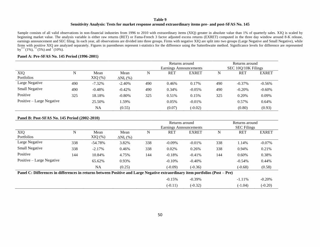
50

Table 9

Sensitivity Analysis: Tests for market response around extraordinary items pre- and post-SFAS No. 145

Sample consists of all valid observations in non-financial industries from 1996 to 2010 with extraordinary items (XIQ) greater in absolute value than 1% of quarterly sales. XIQ is scaled by

beginning market value. The analysis variable is either raw returns (RET) or Fama-French 3 factor adjusted excess returns (EXRET) computed in the three day window around 8-K release,

earnings announcement and SEC filing. In each year, all observations are divided into three groups. Firms with negative XIQ are split into two groups (Large Negative and Small Negative), while

firms with positive XIQ are analyzed separately. Figures in parentheses represent t-statistics for the difference using the Satterthwaite method. Significance levels for difference are represented

by*** (1%), **

(5%) and * (10%).

Panel A: Pre-SFAS No. 145 Period (1996-2001)

Returns around

Earnings Announcements Returns around

SEC 10Q/10K Filings XIQ

Portfolios N Mean

XIQ (%) Mean

NIt (%) N RET EXRET N RET EXRET

Large Negative 490 -7.32% -2.40% 490 0.46% 0.17% 490 -0.37% -0.56%

Small Negative 490 -0.48% -0.42% 490 0.34% -0.05% 490 -0.20% -0.60%

Positive 325 18.18% -0.80% 325 0.51% 0.15% 325 0.20% 0.09%

Positive – Large Negative 25.50% 1.59%

0.05% -0.01%

0.57% 0.64%

NA (0.55)

(0.07) (-0.02)

(0.80) (0.93)

Panel B: Post-SFAS No. 145 Period (2002-2010)

Returns around

Earnings Announcements Returns around

SEC Filings XIQ

Portfolios N Mean

XIQ (%) Mean

NIt (%) N RET EXRET N RET EXRET

Large Negative 338 -54.78% 3.82% 338 -0.09% -0.01% 338 1.14% -0.07%

Small Negative 338 -2.17% 0.46% 338 0.02% 0.26% 338 0.94% 0.21%

Positive 144 10.84% 4.75% 144 -0.18% -0.41% 144 0.60% 0.38%

Positive – Large Negative 65.62% 0.93%

-0.10% -0.40%

-0.54% 0.44%

NA (0.25)

(-0.09) (-0.36)

(-0.68) (0.58)

Panel C: Differences in differences in returns between Positive and Large Negative extraordinary item portfolios (Post – Pre)

-0.15% -0.39% -1.11% -0.20%

(-0.11) (-0.32) (-1.04) (-0.20)

51

Table 10

Portfolio analyses: Tests for market response around early debt retirements by retirement frequency

The analysis variable is either raw returns (RET) or Fama-French 3 factor adjusted excess returns (EXRET) computed in the three day window around 8-K release, earnings announcement and

SEC filing. DGAIN is after tax gains or losses from extinguishment of debt. For pre-FAS145 period, DGAIN is hand-collected from 10-Q or 10-K. For the post-145 period, DGAIN is equal to

the pre-tax gain or loss from debt retirement (DTEPQ) from the Compustat FUNDQ database, adjusted for taxes using the firm specific tax rate. DGAIN is deflated by lagged market value. NI

the seasonally-adjusted earnings surprise. In each year, all observations are divided into three groups. Firms with negative DGAIN are split into two groups (Large Negative and Small Negative),

while firms with positive DGAIN are analyzed separately. Figures in parentheses represent t-statistics for the difference using the Satterthwaite method. Significance levels for difference are

represented by*** (1%), **

(5%) and * (10%).

Panel A: Two or less retirements in both the pre- and post-SFAS No. 145 period

Pre-SFAS No. 145 Period

Returns around

SEC 8-K Filings Returns around

Earnings Announcements Returns around

SEC 10Q/10K Filings DGAIN

Portfolios N Mean

DGAIN (%) Mean

NIt (%) N RET EXRET N RET EXRET N RET EXRET

Large Negative 33 -6.26% -6.28% 18 1.75% 1.68% 33 -0.84% -0.83% 33 -0.34% -0.64% Small Negative 33 -0.56% -0.45% 23 -1.26% -0.93% 33 1.01% 1.16% 33 0.17% -0.14% Positive 22 6.03% 3.33% 11 -1.23% -0.01% 22 -0.32% -0.34% 22 1.35% 0.79% Positive – Large Negative

12.28% 9.61%

-2.98% -1.69%

0.52% 0.49%

1.68% 1.43%

t-statistics

NA (3.46) ***

(-2.30) ** (-0.78)

(0.24) (0.23)

(0.75) (0.86)

Post-SFAS No. 145 Period

Returns around

SEC 8-K Filings Returns around

Earnings Announcements Returns around

SEC 10Q/10K filings DGAIN

Portfolios N Mean

DGAIN (%) Mean

NIt (%) N RET EXRET N RET EXRET N RET EXRET

Large Negative 36 -22.46% -0.95% 22 1.44% 0.55% 36 -2.72% -2.64% 36 -3.15% -3.27% Small Negative 36 -0.63% 0.36% 26 -1.04% -0.66% 36 0.02% -0.17% 36 0.66% 0.54% Positive 17 37.81% 12.76% 6 8.89% 6.56% 17 6.09% 5.94% 17 10.36% 9.72% Positive – Large Negative

13.71%

7.45% 6.01%

8.81% 8.59%

13.51% 12.99%

t-statistics

NA (0.66)

(1.98) ** (0.99)

(1.89) * (2.09) **

(3.31) ** (2.02) **

Differences in differences in returns between Positive and Large Negative DGAIN firms (Post – Pre) 4.10% 10.43% 7.70% 8.29% 8.10% 11.83% 11.56%

(0.20) (2.62) *** (1.19) (1.61) (1.75) * (2.54) ** (1.74) *

52

Table 10 (Cont’d)

Portfolio analyses: Tests for market response around early debt retirements by retirement frequency

Panel B: More Than two retirements in both the pre- and post-SFAS No. 145 period

Pre-SFAS No. 145 Period

Returns around

SEC 8-K Filings Returns around

Earnings Announcements Returns around

SEC 10Q/10K Filings DGAIN

Portfolios N Mean

DGAIN (%) Mean

NIt (%) N RET EXRET N RET EXRET N RET EXRET

Large Negative 60 -2.47% -2.74% 29 0.23% 0.24% 60 0.66% 0.40% 60 0.79% 0.77%

Small Negative 61 -0.30% -0.88% 17 0.55% 1.02% 61 1.38% 1.52% 61 -0.05% -0.23%

Positive 49 14.06% 4.00% 4 0.05% 0.62% 49 -0.76% -1.05% 49 0.65% 0.59%

Positive – Large Negative

16.52% 6.75%

-0.18% 0.38%

-1.42% -1.46%

-0.14% -0.19%

t-statistics

NA (0.64)

(-0.03) (0.07)

(-0.68) (-0.74)

(-0.08) (-0.11)

Post-SFAS No. 145 Period

Returns around

SEC 8-K Filings Returns around

Earnings Announcements Returns around

SEC 10Q/10K Filings DGAIN

Portfolios N Mean

DGAIN (%) Mean

NIt (%) N RET EXRET N RET EXRET N RET EXRET

Large Negative 99 -3.81% -0.34% 29 -0.60% -0.99% 99 -2.43% -2.55% 99 -2.89% -2.79% Small Negative 99 -0.42% 0.49% 23 -0.44% 0.59% 99 0.69% 0.80% 99 -0.88% -0.38% Positive 55 30.16% 1.43% 9 1.11% -0.85% 55 2.55% 2.52% 55 1.70% 2.56% Positive – Large Negative

33.97% 1.77%

1.71% 0.13%

4.98% 5.07%

4.59% 5.34%

t-statistics

NA (0.25)

(0.33) (0.03)

(1.65) * (1.71) *

(2.08) * (2.53) **

Differences in differences in returns between Positive and Large Negative DGAIN firms (Post – Pre) -4.98% 1.89% -0.25% 6.40% 6.53% 4.73% 5.53% (-0.39) (0.23) (-0.03) (1.74) * (1.84) * (1.68) * (2.01) **

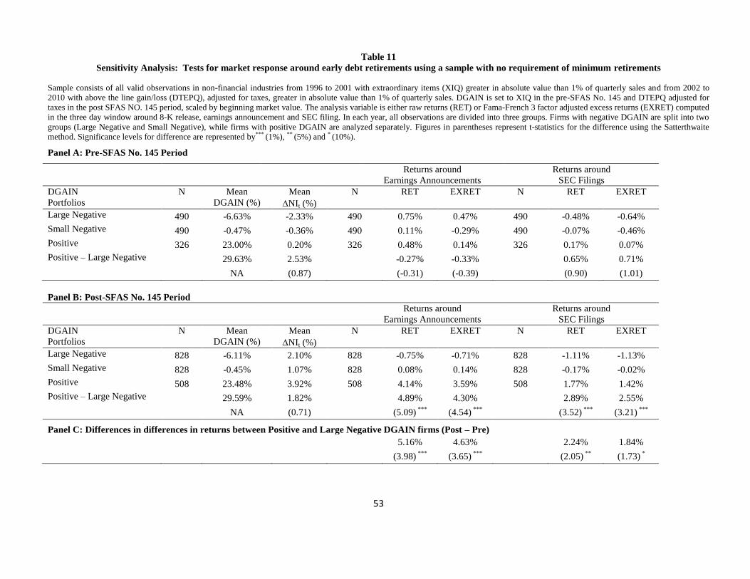
53

Table 11

Sensitivity Analysis: Tests for market response around early debt retirements using a sample with no requirement of minimum retirements

Sample consists of all valid observations in non-financial industries from 1996 to 2001 with extraordinary items (XIQ) greater in absolute value than 1% of quarterly sales and from 2002 to

2010 with above the line gain/loss (DTEPQ), adjusted for taxes, greater in absolute value than 1% of quarterly sales. DGAIN is set to XIQ in the pre-SFAS No. 145 and DTEPQ adjusted for

taxes in the post SFAS NO. 145 period, scaled by beginning market value. The analysis variable is either raw returns (RET) or Fama-French 3 factor adjusted excess returns (EXRET) computed

in the three day window around 8-K release, earnings announcement and SEC filing. In each year, all observations are divided into three groups. Firms with negative DGAIN are split into two

groups (Large Negative and Small Negative), while firms with positive DGAIN are analyzed separately. Figures in parentheses represent t-statistics for the difference using the Satterthwaite

method. Significance levels for difference are represented by*** (1%), **

(5%) and * (10%).

Panel A: Pre-SFAS No. 145 Period

Returns around

Earnings Announcements Returns around

SEC Filings DGAIN

Portfolios N Mean

DGAIN (%) Mean

NIt (%) N RET EXRET N RET EXRET

Large Negative 490 -6.63% -2.33% 490 0.75% 0.47% 490 -0.48% -0.64%

Small Negative 490 -0.47% -0.36% 490 0.11% -0.29% 490 -0.07% -0.46%

Positive 326 23.00% 0.20% 326 0.48% 0.14% 326 0.17% 0.07%

Positive – Large Negative 29.63% 2.53%

-0.27% -0.33%

0.65% 0.71%

NA (0.87)

(-0.31) (-0.39)

(0.90) (1.01)

Panel B: Post-SFAS No. 145 Period

Returns around

Earnings Announcements Returns around

SEC Filings DGAIN

Portfolios N Mean

DGAIN (%) Mean

NIt (%) N RET EXRET N RET EXRET

Large Negative 828 -6.11% 2.10% 828 -0.75% -0.71% 828 -1.11% -1.13%

Small Negative 828 -0.45% 1.07% 828 0.08% 0.14% 828 -0.17% -0.02%

Positive 508 23.48% 3.92% 508 4.14% 3.59% 508 1.77% 1.42%

Positive – Large Negative 29.59% 1.82%

4.89% 4.30%

2.89% 2.55%

NA (0.71)

(5.09) *** (4.54)

***

(3.52) *** (3.21)

***

Panel C: Differences in differences in returns between Positive and Large Negative DGAIN firms (Post – Pre) 5.16% 4.63% 2.24% 1.84%

(3.98) *** (3.65)

*** (2.05) ** (1.73)

*

54

Table 12

Sensitivity Analysis: Tests for market response around early debt retirements using unrestricted sample

Sample consists of all valid observations in non-financial industries from 1996 to 2001 with extraordinary items (XIQ) and from 2002 to 2010 with above the line gain/loss (DTEPQ), adjusted

for taxes. DGAIN is set to XIQ in the pre-SFAS No. 145 and DTEPQ adjusted for taxes in the post SFAS NO. 145 period, scaled by beginning market value. The analysis variable is either raw

returns (RET) or Fama-French 3 factor returns (EXRET) computed in the three day window around 8-K release, earnings announcement and SEC filing. In each year, all observations are

divided into three groups. Firms with negative DGAIN are split into two groups (Large Negative and Small Negative), while firms with positive DGAIN are analyzed separately. Figures in

parentheses represent t-statistics for the difference using the Satterthwaite method. Significance levels for difference are represented by*** (1%), **

(5%) and * (10%).

Panel A: Return Trend in the Pre-SFAS No. 145 Period

Returns around

Earnings Announcement Returns around

SEC filing DGAIN

Portfolios N Mean

DGAIN (%) Mean

NIt (%) N RET EXRET N RET EXRET

Large Negative 1216 -2.97% -1.19% 1216 0.18% -0.04% 1216 -0.19% -0.34% Small Negative 1216 -0.13% 0.07% 1216 0.45% 0.24% 1216 0.65% 0.34% Positive 891 6.35% 3.21% 891 0.30% -0.03% 891 -0.29% -0.47% Positive – Large Negative 9.31% 4.40%

0.12% 0.02%

-0.10% -0.13%

NA (3.64)***

(0.25) (0.04)

(-0.25) (-0.32)

Panel B: Return Trend in the Post-SFAS No. 145 Period

Returns around

Earnings Announcement Returns around

SEC filing DGAIN

Portfolios N Mean

DGAIN (%) Mean

NIt (%) N RET EXRET N RET EXRET

Large Negative 2368 -2.24% 1.66% 2368 -0.31% -0.34% 2368 -0.56% -0.61% Small Negative 2369 -0.07% 1.04% 2369 0.22% 0.23% 2369 0.01% 0.08% Positive 1468 4.99% 3.05% 1468 2.21% 1.97% 1468 0.80% 0.53% Positive – Large Negative 7.23% 1.39%

2.52% 2.31%

1.36% 1.14%

(1.41)

(5.38) *** (5.08)

***

(3.59) *** (3.14)

***

Panel C: Differences in differences in returns between Positive and Large Negative DGAIN firms (Post – Pre) 2.40% 2.29% 1.46% 1.27% (3.53)

*** (3.47) *** (2.61)

*** (2.33) ***