Does Financial Development Mitigate Negative Effects of ...

_____________________________________________________________________CREDIT Research Paper

No. 00/1_____________________________________________________________________

Does Financial Development MitigateNegative Effects of Policy Uncertainty

on Economic Growth?

by

Robert Lensink

_____________________________________________________________________

Centre for Research in Economic Development and International Trade,University of Nottingham

The Centre for Research in Economic Development and International Trade is based inthe School of Economics at the University of Nottingham. It aims to promote researchin all aspects of economic development and international trade on both a long term anda short term basis. To this end, CREDIT organises seminar series on DevelopmentEconomics, acts as a point for collaborative research with other UK and overseasinstitutions and publishes research papers on topics central to its interests. A list ofCREDIT Research Papers is given on the final page of this publication.

Authors who wish to submit a paper for publication should send their manuscript tothe Editor of the CREDIT Research Papers, Professor M F Bleaney, at:

Centre for Research in Economic Development and International Trade,School of Economics,University of Nottingham,University Park,Nottingham, NG7 2RD,UNITED KINGDOM

Telephone (0115) 951 5620Fax: (0115) 951 4159

CREDIT Research Papers are distributed free of charge to members of the Centre.Enquiries concerning copies of individual Research Papers or CREDIT membershipshould be addressed to the CREDIT Secretary at the above address.

_____________________________________________________________________CREDIT Research Paper

No. 00/1

Does Financial Development MitigateNegative Effects of Policy Uncertainty

on Economic Growth?

by

Robert Lensink

_____________________________________________________________________

Centre for Research in Economic Development and International Trade,University of Nottingham

The AuthorRobert Lensink is External Fellow of CREDIT and Associate Professor, Faculty ofEconomics, University of Groningen.

____________________________________________________________ Manuscript Received: February 2000

Does Financial Development Mitigate Negative Effects of Policy Uncertainty onEconomic Growth?

ByRobert Lensink

AbstractBy performing a cross-country growth regression for the 1970-1998 period this paper

finds evidence for the fact that countries with a more developed financial sector are

better able to nullify the negative effects of policy uncertainty on per capita economic

growth. This clearly indicates the relevance of financial sector development.

Outline1. Introduction2. Uncertainty, financial development and economic growth3. The policy uncertainty measures and the indicator for financial development4. The method and base model regression results5. Explaining financial market development: estimates with instruments6. Stability analysis7. Conclusions

1

1. INTRODUCTION

The importance of stable and predictable macroeconomic policies for economic growth,

especially for developing countries, has been debated quite extensively in the literature.

Many authors state that the successful implementation of a structural adjustment program

crucially depends on government policies being credible (see, e.g. Rodrik, 1989 and

Calvo, 1988). In line with this, several studies suggest that policy uncertainty has a

negative effect on aggregate investment and economic growth (see Aizenman and

Marion, 1993, and Lensink, Bo and Sterken, 1999).

The literature on financial development and economic growth argues that financial

intermediaries can better manage risk than individual wealth-holders. This implies that

firms in countries with a more developed financial sector are better able to diversify risks,

enabling them to carry out the more risky, but also more productive investment projects.

This suggests that the effect of policy uncertainty on economic growth is dependent on

the development of the financial sector. However, quite remarkable, there are no

empirical studies available that have tried to test this. This paper partly fills this gap by

examining whether a well-developed financial sector may undo the negative effects of

policy uncertainty on economic growth. It investigates whether a given level of policy

uncertainty has a different effect on economic growth in countries with a well-developed

financial sector as compared to countries with a poorly developed financial sector.1 This

is done by performing a Barro (1991) -type cross-country growth regression, in which

different policy uncertainty measures are included, and in which the interaction between

policy uncertainty and financial development is taken into account.

Section 2 surveys relevant literature for the analysis of this paper. I do not present a

formal model, but present several reasons as to why the uncertainty-growth relationship

probably depends on the degree of financial market development. Section 3 explains how

uncertainty and financial sector development is measured. Section 4 describes the

1 It may also be relevant to examine whether financial development affects the degree of uncertainty as such.However, that is not the focus point of this paper.

2

method, and presents regression results of a base model. Section 5 re-estimates the base

model by using instruments for financial market development. This is an important issue

in the new literature on financial market development and economic growth (see Levine,

1997a and Levine, Loayza and Beck, 1999). Section 6 examines the robustness of the

results. Section 7 concludes.

2. UNCERTAINTY, FINANCIAL DEVELOPMENT AND ECONOMIC

GROWTH

The literature on policy uncertainty and economic growth is closely connected to a now

booming research theme regarding the effects of uncertainty on investment. Well-known

references in this field are Lucas and Prescott (1971), Arrow (1968), Abel (1983),

Bernanke (1983), Caballero (1991), Abel and Eberly (1994), Dixit and Pindyck (1994)

and Leahy and Whited (1996). Lensink, Bo and Sterken (2000) present an up to date

overview. The literature shows that the impact of uncertainty on investment depends on

many factors, such as the risk behavior, the production technology in combination with

the market structure, the degree of irreversibility and expandability of investments and the

degree of capital market imperfections. Most models assume that firms are risk-neutral.

Traditionally, these models argue that uncertainty has a positive effect on investment. For

instance, Abel (1993) and more recently Caballero (1991), show that an increase in

(price) uncertainty stimulates investment as long as the marginal revenue product of

capital is a convex function of prices. This is always the case whenever firms are perfectly

competitive and the production function has constant returns to scale. In the case where

firms are not perfectly competitive, and/or the production function does not have constant

returns to scale, the investment-uncertainty sign is not necessarily positive. It depends e.g.

on the degree of irreversibility and expandability of investment.

The modern option approach to invest (Dixit and Pindyck, 1994) argues that investment

is (partly) irreversible due to sunk costs which can not be recovered completely by selling

capital when the investment has been done. In these models the “bad news principle of

irreversible investment” holds. This principle implies that higher uncertainty does not

symmetrically affect outcomes in the good and bad states. For instance, if demand is

unexpectedly high (good state), the firm can easily increase the capital stock. However, if

the demand is unexpectedly low (bad state) the firm can not undo the investment decision

3

due to the irreversibility of investment. Therefore only bad news will affect the current

investment decision and hence higher uncertainty leads to a decrease in immediate

investment. Due to the close connection between investment and economic growth, an

increase in uncertainty would probably have also a negative effect on economic growth.

In addition to the effect of the degree of irreversibility on the investment-uncertainty

relationship, the development of the financial market matters. Early contributions to the

theory of financial intermediation and economic growth are due to Schumpeter (1939)

and Gurley and Shaw (1955). They have stressed that financial intermediation could

contribute to economic growth by mobilizing saving and increasing the productivity of

capital. The relationship between financial markets and economic growth is now one of

the most important issues in development economics. There are too many studies to

mention, but see Levine and Renelt (1992), King and Levine (1993), Hermes and Lensink

(1996 and 1998), Levine (1997) and Levine, Loayza and Beck (1999) for some recent

theoretical and empirical contributions. The recent literature argues that financial

intermediaries primarily contribute to enhanced economic growth by providing a more

efficient allocation of resources. Financial intermediaries have larger pools of financial

resources as compared to individual wealth holders, so that they are better able to reduce

the adverse impact of risks of failing projects on the total returns earned by diversifying

their portfolio of investments financed. In other words, financial intermediaries are able to

diversify and pool risks. Moreover, financial intermediation leads to a reduction of

liquidity risks. Agents are uncertain about future liquidity needs. Therefore, agents in an

uncertain world without financial intermediaries will hold a substantial part of their wealth

in liquid assets, probably yielding low returns. Hence, without a well-developed financial

sector, many projects with high returns in the long-run will probably not be carried out in

an uncertain world. Financial intermediaries may contribute to enhanced resource

allocation by agglomerating the saving of many individuals and funnel these resources to

high return, low liquidity investment projects. Therefore, financial intermediaries can both

reduce liquidity risks for individuals and at the same time increase investment efficiency.

Moreover, in case of uncertain demand or productivity shocks in the macroeconomic

environment investing in firms by individual wealth holders is highly risky, and hence will

probably not take place. Since financial intermediaries, by holding diversified portfolios,

are better able to reduce risks of highly fluctuating returns, a well-developed financial

sector may contribute to financing a higher volume and efficiency of investment. In

4

addition, if capital markets are imperfect, firms can not issue more equity by which risk

can be absorbed (Greenwald and Stiglitz, 1990). Therefore, if capital markets are

imperfect, firms will probably lower investment when uncertainty about profitability

increases. Ghosal and Loungani (1997) argue that the uncertainty-investment relationship

depends on the degree of capital market imperfections. Peeters (1997), in a study on

investment for Belgian and Spanish firms, provides empirical evidence for the fact that

financial development matters for the uncertainty-investment relationship. She shows that

uncertainty only has a negative effect on investment of firms that are relatively financially

constraint.

The aforementioned literature on financial market development and economic growth

suggests that the impact of uncertainty on economic growth is dependent on the

development of the financial sector of a country. The reason is that a well-developed

financial system can manage risks more efficiently. In the case of stock markets, the risk

diversification will be direct, whereas it is indirect in the case of commercial banks. In the

remainder of the paper the effect of financial market development on the policy

uncertainty-economic growth relationship will be tested. The next section explains how I

have measured uncertainty and financial development.

3. THE POLICY UNCERTAINTY MEASURES AND THE INDICATOR FOR

FINANCIAL DEVELOPMENT

In the literature the following methods to measure uncertainty are used (see Lensink, Bo

and Sterken, 2000):

1) The standard deviation of the variable under consideration;

2) The standard deviation of the unpredictable part of a stochastic process;

3) The standard deviation from a geometric Brownian process;

4) The General AutoRegressive Conditional Heteroskedastic (GARCH) model of

volatility

5) The standard deviation derived from Survey Data.

The application of the third method (geometric Brownian motion) requires continuous

data, which makes the method not applicable to this paper. The fifth method, based on

5

survey data, is also almost impossible to use in this paper since the regressions are done

for a cross-section of almost 100 countries. It would need an enormous amount of

respondents to obtain reliable data. This leaves three possibilities. In this paper

uncertainty will primarily be measured using the second method. This method is

somewhat more sophisticated than the first method. Moreover, the fourth method, based

on the conditional variance estimated from a General Autoregressive Conditional

Heteroskedastic (GARCH)-type model, is especially relevant for high frequency data

which display clustering effects. Since the data set used consists of annual observations,

estimating uncertainty by the variance of the unpredictable part of a stochastic process is

appropriate. In order to test the sensitivity of the results for the measurement of

uncertainty, regressions are presented in which uncertainty is measured according to the

first or fourth method (see Section 6).

The preferred method to measure uncertainty works as follows. First specify and

estimate a forecasting equation to determine the expected part of the variable under

consideration. Next, the standard deviation of the unexpected part of the variable, i.e. the

residuals from the forecasting equation, is used as the measure of uncertainty. This

approach has also been used by e.g. Aizenman and Marion (1993), Ghosal (1995), and

Ghosal and Loungani (1996). Differences in the measurement of the uncertainty proxy

mostly stem from the way in which the forecasting equation is formulated. I follow the

customary approach and use a first-order autoregressive process, extended with a time

trend and a constant, as the forecasting equation:

Pt = a1 + a2T + a3Pt-1 + et,

where Pt is the variable under consideration, T is a time trend, a1 is an intercept, a3 is

the autoregressive parameters and et is an error term.

6

The above equation is estimated for all countries in the data set (see Appendix2), over

the 1970-1998 period.2 By calculating, for each country, the standard deviation of the

residuals for the entire sample period, a proxy for uncertainty is derived. Two types of

uncertainty can be identified to measure the credibility with regard to monetary and

fiscal policies, respectively (see Appendix1 for a list of variables):

UINFL: uncertainty with respect to inflation (P variable is the yearly inflation rate)

UGOV: uncertainty with respect to government consumption (P variable is

government expenditures divided by GDP)

2 I also estimated the forecasting equation by using a second and a third order autoregressive process withtrend. Results were similar. For reasons of space it is not possible to present the estimation results for allcountries.

7

The next step consists of the construction of the financial ratio. In several papers,

financial ratios are suggested to describe the size and structure of, and/or the

distribution, of loans through the financial sector. These papers claim that these ratios

contain information about the services provided by the financial institutions (see,

among others, King and Levine, 1993). Levine, Loayza and Beck (1999) distinguish

three measures: 1) Liquid liabilities of the financial system divided by GDP; 2) The

ratio of commercial bank assets divided by commercial bank plus central bank assets

and 3) the value of credits by financial intermediaries to the private sector divided by

GDP.

Levine, Loayza and Beck (1999) prefer the third measure since it isolates credit issued

to the private sector and hence gives information about the amount of loans that are

directed to the private sector. I also use credit to the private sector as a percentage of

GDP (CREDPR) as a measure for financial development. It should be noted that my

measure for financial sector development differs somewhat from the

one used by Levine, Loayaza and Beck (1999). The main difference is that their

measure excludes credits issued by the monetary authorities and government agencies.

I do not use their measure since it is only available for a much smaller data set. Both

measures are however strongly correlated (a correlation coefficient of about 90%).

Moreover, in Section 6 I will present some estimates in which I use the measure

developed by Levine, Loayaza and Beck in order to test the sensitivity of the results.

One may argue that the financial market indicator I use does not provide much

information about the quality of services of financial intermediaries. However, since

there are no better financial market indicators available that deal explicitly with the

quality of financial institutions, at the least for a large cross-section of countries, there

was not much of a choice.

4. THE METHOD AND BASE MODEL REGRESSION RESULTS

The aim of this paper is to examine whether possible growth reducing effects of policy

uncertainty may be nullified by financial sector development. A first question is whether it

is more appropriate to use a pure cross-section analysis, or to do the estimates on a panel

of countries. In the growth regressions literature both approaches are popular. The choice

8

depends on several factors, such as the aim of the study, data availability and the period

over which certain effects are expected to take place. If the panel technique is chosen, it is

common to divide the period for which data are available in different sub-periods, usually

of five years. The estimates are then performed on averages for the five year periods. For

our study an argument in favor of the panel approach using five year averages would be

that policies might change in short period of times. On the other hand, a strong argument

for the cross-section approach is that a reasonable estimate of the uncertainty proxy needs

a long estimation period. The variables used for the uncertainty measure are only available

on a yearly basis. Since the uncertainty proxy is calculated by taking the standard

deviation of the unpredicted part and the forecasting equation is based on an

autoregressive process, a five year period would certainly be too short. For this reason I

decided to perform a pure cross-country analysis using data averaged over the 1970-1998

period.

In line with most of the cross-country growth literature, the dependent variable is the

growth rate of real per capita Gross Domestic Product (GRO). This variable is calculated

from an updated series on real GDP per capita figures originally provided by Summers

and Heston. I start the analysis by estimating the following equations:

(1) GRO=α1+ α2 LGDPPCI+α3SECI+α4CREDPR+α5UGOV+α6UGOV*CREDPR+µ

(2) GRO = α7 + α8 LGDPPCI+α9SECI+α10CREDPR+α11UINFL+α

12UINFL*CREDPR+µ

Where GRO is the per capita growth rate of GDP over the 1970-1998 period; LGDPPCI

is the logarithm of the 1970 of per capita GDP; SECI is the 1970 secondary-school

enrollment rate and µ is an error term.

The interaction term is included in order to capture the importance of financial

development for the effects of policy uncertainty on economic growth.3 A closer look at

equation (1) may explain matters. Differentiating (1) with respect to UGOV gives:

3 The approach is in line with that of Ghosal (1991)

9

d (GRO)/d UGOV = α5+α6*CREDPR

This clearly shows that the above formulation implies that the growth effects of

uncertainty depend on financial development. In line with most empirical analysis, in

which it is shown that uncertainty negatively affects economic growth, I expect that α5 <

0. In addition, I assume that countries with a more developed financial system are better

able to insure themselves against negative uncertainty effects. Hence, I expect that α6 >0.

If α5 < 0 and α6 >0, the threshold level of financial development above which uncertainty

has a positive effect on economic growth can be calculated by setting the first derivative

equal to zero. The threshold level then equals: -α5 /α6.

In order to come up with a reasonable base model I include LGDPPCI and SECI in the

equations. These variables are shown to have a robust and significant impact on economic

growth, and hence are included in most recent growth regression studies (see, for

instance, Sala-i-Martin, 1997a and 1997b).4 LGDPPC is included to account for the

conditional convergence effect. The logarithmic form is suggested by theoretical

derivations of the convergence rate (see Barro and Sala-i-Martin, 1995). The sign is

expected to be negative. SECI proxies for the initial stock of human development. The

sign is expected to be positive. I also include CREDPR since the significance of the

interaction term may be the result of the omission of other variables, in particular

CREDPR itself. Hence, it is important to include the interaction term as well as both

individual terms separately in the equation. This makes it possible to jointly examine the

individual as well as the interactive effects of uncertainty and financial market

development on economic growth.5

Before presenting the regression results of the base models descriptive statistics of the

main variables are given in Table 1. The table shows that for some variables the mean

4 It should, however, be noted that results are somewhat mixed with respect to the robustness of

SECI.

5 Some growth regressions include the investment to GDP ratio in the base model. However, since investmentis clearly endogenous this is somewhat problematic. For that reason I do not present results in which theinvestment to GDP ratio is included as an additional variable.

10

substantially differs from the median. Hence, some variables suffer from skewness. This is

a normal phenomenon in cross-section and panel studies. It signals that in estimating the

models one should be cautious about nonnormality of the residuals.6

Table 1: Descriptive statistics main variables

GRO LGDPPCI SECI UGOV UINFL CREDPR ICREDPR RULELAW

Mean 1.434 7.669 32.976 1.412 118.403 38.871 34.697 0.149

Median 1.579 7.615 24.000 0.986 6.897 27.496 28.670 -0.013

Maximum 6.476 9.284 102.000 9.123 4240.660 155.216 106.880 1.939

Minimum -4.356 5.690 1.000 0.244 1.067 2.665 -1.454 -2.153

Std. Dev 1.926 0.996 27.413 1.238 538.829 25.881 20.502 0.989

Skewness -0.149 0.046 0.677 3.297 6.159 1.549 1.084 0.127

Kurtosis 3.939 1.864 2.178 18.972 43.661 6.878 4.538 2.023

Jarque-Bera 3.433 4.598 8.874 1057.505 6392.763 87.251 25.034 3.608

Obs. 85 85 85 85 85 85 85 85

Statistics are based on a balanced sample

The regression results of the two base models are presented as equation (1) and equation

(2) in Table 2. LGDPPCI appears to be highly significant with the correct sign. The

coefficient on LGDPPCI is between 1 and 1.5, which suggests that for each country the

convergence to its steady state is achieved at a rate between 1% and 1.5% per year. This

is in line with other cross-country studies (see Sala-i-Martin, 1997b). SECI is also

significant with the correct sign. The coefficient is about 0.05, which is also in line with

other recent growth regressions. The base regressions suggest that policy uncertainty has

an individual significant negative effect on growth performance. The coefficients for

UINFL, and UGOVC are highly significant with a negative sign. Most importantly are the

results for the interaction terms. They are highly significant in both cases, with a positive

sign. This clearly confirms the hypothesis that countries with a more developed financial

sector, as measured both by CREDPR, are better able to undo the growth reducing

6 For all estimates done I tested whether the residuals were normally distributed using the Jarque-Bera teststatistic. According to this test, the residuals were normally distributed for all regressions.

11

effects of policy uncertainties. Finally, the base regressions suggest that development of

the financial sector does not have an individual significant effect on economic growth:

CREDPR is insignificant in both cases.

Table 2: Base model estimates on financial development, uncertainty and economicgrowth

1 2

LGDPPCI -1.179 (-3.65) -1.112 (-3.56)

SECI 0.046 (3.87) 0.054 (4.52)

CREDPR 0.008 (0.75) 0.014 (1.17)

UGOV -0.781 (-2.94)

UGOV*CREDPR 0.025 (2.76)

UINFL -0.001 (-14.86)

UINFL*CREDPR 4.96E-05 (8.01)

CONSTANT 8.807 (4.22) 7.813 (3.78)

Statistics

R2 0.38 0.32

F 12.35 9.21

Obs. 94 87

Dependent variable: GRO. t-Statistics between parenthesis. t-Statistics are based on WhiteHeteroskedasticity-Consistent Standard Errors. R2 is the adjusted R-squared.

5 EXPLAINING FINANCIAL MARKET DEVELOPMENT: ESTIMATES

WITH INSTRUMENTS

An important issue in the recent literature on financial development and economic growth

is the endogeneity of financial sector development. The causality between growth and

financial sector development may run from growth to financial sector development, which

may have important implications for the base regressions presented in the previous

section. In these regressions it is implicitly assumed that the causality runs from financial

market development to economic growth. A way around this problem is to use

instruments for financial sector development. In this way it is possible to extract the

exogenous component of financial sector development and to examine whether the

exogenous component of financial intermediary development is positively correlated with

12

economic growth. The problem is to find instruments which are uncorrelated with the

error and highly correlated with the dependent variable, in this case with CREDPR.

Levine (1997a) and Levine, Loayza and Beck (1999) argue that indicators with respect to

the legal system and the regulatory environment are appropriate instruments for financial

sector development. They suggest to use indicators for the legal origin of the country and

the rule of law.7 With respect to the indicators for regulatory environment I had a choice

between six measures: GRAFT, PINST, RULELAW, REGBURDEN, VOICE and

GOVEFF (see Appendix1).8 Table 3 shows that these six indicators are strongly

correlated. Therefore, I only used RULELAW as instrument. The results are not affected

by this choice.

Table 3: Correlation matrix aggregate governance indicators

GRAFT PINST RULELAW REGBURDEN VOICE GOVEFF

GRAFT 1.00 0.75 0.88 0.68 0.76 0.92

PINST 1.00 0.88 0.68 0.68 0.79

RULELAW 1.00 0.74 0.72 0.89

REGBURDEN 1.00 0.75 0.76

VOICE 1.00 0.77

GOVEFF 1.00

7 Levine, Loayza and Beck use legal origin indicators for countries with predominantly English, French,German or Scandinavian legal origin.

8 It should be noted that these indicators are not exactly the same as the indicators used by Levine, Loayza andBeck (1999). However, they are comparable. I have not used their indicators since they were only available fora much smaller data set. The set of indicators I use is available for almost all countries in the sample.

13

In addition to the six aggregate governance indicators, I also tested the relevance of some

legal origin indicators. I examined the relevance of British, French, Scandinavian, German

or Socialist legal origin. Finally, again in line with Levine (1997a) and Levine, Loayza and

Beck (1999) I included LGDPPCI as additional instrument. In Table 4 estimation results

concerning the instruments are presented. It appears that RULELAW and LGDPPCI are

highly significant in all regressions with CREDPR as the independent variable (equations

1, 2 and 3). In the case where all legal origin indicators are included not one of them is

significant (equation 2). However, when one of them is ignored LEGGERMAN, the

dummy for countries with a German legal origin becomes significant (see equation 3).

Based on these regression results I use RULELAW, LGDPPCI, LEGGERMAN and a

constant as instruments for CREDPR. From this regression I obtain a fitted variable of

CREDPR, called ICREDPR.

Table 4: Determination instruments for financial development

1 2 3 4

LGDPPCI 6.782 (3.58) 6.556 (3.62) 6.477 (3.56) 12.588 (3.22)

RULELAW 13.749 (5.93) 11.708 (4.80) 11.800 (5.26) 7.843 (2.75)

LEGBRITISH -16.475 (-1.19)

LEGFRENCH -19.222 (-1.42)

LEGSOCIALIST -28.549 (-1.58)

LEGSCAN -21.878 (-1.29)

LEGGERMAN 27.152 (1.139) 46.049 (2.42) 46.513 (3.07)

CONSTANT -19.641 (-1.38) -18.352 (-1.33) -67.756 (-2.27)

14

Statistics

R2 0.44 0.52 0.52 0.66

F 51.88 24.31 47.64 44.24

Obs. 131 128 128 69

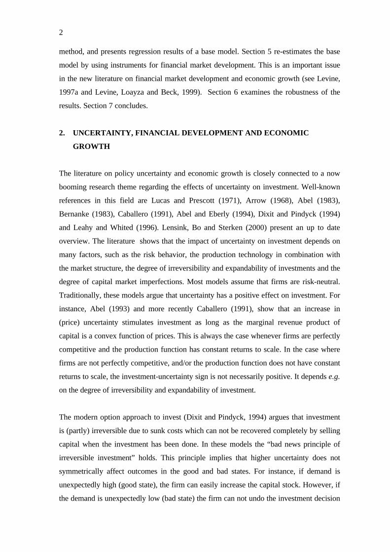
Dependent variable in equation 1, 2 and 3 is CREDPR. In equation 4 the dependent variable isLCREDPR. t-Statistics between parenthesis. t-Statistics are based on White Heteroskedasticity-Consistent Standard Errors. R2 is the adjusted R-squared.

The next step is to re-estimate the two base equations by replacing CREDPR by its fitted

value ICREDPR . The results are given by equations 1 and 2 in Table 5. It appears that

the main results so far still hold: uncertainty has an individual negative effect on economic

growth and the negative effect of uncertainty on economic growth becomes smaller the

more developed the financial sector of a country. There is one main difference with the

estimates presented before: the individual effect of the exogenous component of financial

sector development (ICREDPR) is now also significant with the correct sign.

Table 5: Estimates with instruments for financial market development

1 2 3 4

LGDPPCI -1.582 (-5.43)

-1.273 (-4.35) -1.566 (-5.15)

-1.278 (-4.33)

SECI 0.027 (2.42) 0.033 (2.96) 0.028 (2.53) 0.033 (2.95)

ICREDPR 0.033 (1.80) 0.053 (2.61) 0.033 (1.78) 0.054 (2.60)

UGOV -1.572 (-5.49)

-1.536 (-4.78)

UGOV*ICREDPR 0.042 (4.46) 0.042 (4.38)

UINFL -0.001 (-9.07) -0.001 (-1.68)

UINFL*ICREDPR 3.21E-05(4.10)

3.12E-5 (5.36)

15

GOV -0.015 (-0.47)

INFL 0.0005 (0.21)

CONSTANT 12.026 (5.99) 8.333 (4.45) 12.042 (6.02) 8.356 (4.42)

Statistics

R2 0.50 0.38 0.50 0.38

F 19.20 11.42 15.88 9.40

Obs. 92 85 92 85


Finally, I include the average government expenditures to GDP ratio (GOV) and the

average inflation rate (INFL) in the equations containing UGOV and UINFL respectively.

These results are given by equations 3 and 4 in Table 5. The inclusion of GOV appears to

have no effect on the regression results. It is remarkable that GOV is insignificant,

whereas UGOV is strongly significant with a negative sign. This indicates that absence of

credibility with respect to fiscal policy in the form of government expenditures is much

more negative for economic growth than an increase in government expenditures as such.

In the case where INFL is added to the model, the significance of UINFL drops

substantially. This suggests that the variability of inflation is strongly correlated with the

level of the inflation rate, which is a well-known phenomenon.

6. STABILITY ANALYSIS

To test the reliability of the above results, I conduct several stability tests. I start by

testing whether the results are sensitive to the use of CREDPR as financial sector

indicator. I replace CREDPR by LCREDPR, which is the preferred indicator for financial

sector development of Levine, Loyaza and Beck (1999). As explained before, the main

difference concerns the exclusion of credit issued by the monetary authorities and

government agencies. The disadvantage of using LCREDPR is that it is not available for

the entire group of countries in the cross-section I use. In line with the analysis before, I

16

use instruments for financial sector development. This comes down to replacing

LCREDPR by its fitted value, LICREDPR, from an equation in which LGDPPCI,

RULELAW and LEGGERMAN are used as instruments (see equation 4 in Table 4). The

results of the regressions using LICREDPR in stead of ICREDPR are presented in Table

6. The message which comes out of these regressions is the same as before: policy

uncertainty has a negative individual effect on growth and a more developed financial

sector may partly undo the negative effects of policy uncertainty on economic growth.

Table 6: Estimates using an alternative measure for financial development

1 2 3 4

LGDPPCI -1.999 (-5.30) -1.493 (-3.24) -1.990 (-5.23) -1.535 (-3.29)

SECI 0.030 (2.25) 0.036 (2.43) 0.027 (1.74) 0.037 (2.47)

LICREDPR 0.015 (0.92) 0.043 (1.87) 0.016 (0.93) 0.044 (1.87)

UGOV -2.581 (-7.60) -2.599 (-7.84)

UGOV*LICREDPR 0.062 (7.65) 0.060 (6.45)

UINFL -0.001 (-9.24) -0.002 (-3.70)

UINFL*LICREDPR 3.46E-05 (3.70) 3.22E-05 (3.35)

GOV 0.018 (0.50)

INFL 0.002 (1.20)

CONSTANT 16.370 (6.06) 10.413 (3.42) 16.177 (5.87) 10.649 (3.46)

Statistics

R2 0.62 0.42 0.62 0.41

F 19.25 8.98 15.81 7.44

Obs. 56 56 56 56


Next, I test whether the results are sensitive to the measurement method of policy

uncertainty. I proxy uncertainty using two alternative methods. First, I estimate

uncertainty by using a GARCH approach. The uncertainty proxies are then defined as

UGOV1 and UINFL1. More specifically, I re-estimate the forecasting equation presented

in Section 2 by a GARCH(1,1) model. A GARCH model assumes that the variance of the

error terms is not constant over time. The technique comes down to taking into account

an additional equation for the conditional variance which depends on a lagged value of

the squared error terms and a lagged value of the conditional variance. The model is

17

estimated using the maximum-likelihood technique. As proxy for uncertainty I use, for all

countries in the data set, the standard deviation of the residuals of the forecasting

equation for the entire sample period.9 Note that the forecasting equation is called the

mean equation in case of a GARCH model. Moreover, as an alternative sensitivity test, I

proxy uncertainty by the standard deviation of government expenditures over GDP and

the inflation rate, respectively. These proxies are defined as UGOV2 and UINFL2. The

results using the alternative estimates for uncertainty are presented in Table 7. It appears

that the main conclusion still holds. The use of a GARCH model to determine the

uncertainty proxy does not seem to affect the results. This can be explained by the fact

that the sample is based on yearly data for which no clustering effects are expected.

Table 7: Alternative measures for uncertainty

1 2 3 4

LGDPPCI -1.588 (-5.53) -1.329 (-4.53) -1.275 (-4.34) -1.279 (-4.35)

SECI 0.029 (2.56) 0.024 (2.25) 0.033 (2.95) 0.033 (2.96)

ICREDPR 0.033 (1.76) 0.047 (1.93) 0.053 (2.62) 0.053 (2.62)

UGOV1 -1.471 (-5.03)

UGOV1*ICREDPR 0.042 (4.22)

UGOV2 -0.509 (-3.26)

9 Alternatively one could argue that it would also be appropriate to use the mean or the median of theconditional variances over the sample period as the proxy for uncertainty.

18

UGOV2*ICREDPR 0.009 (1.91)

UINFL1 -0.0008 (-8.89)

UINFL1*LICREDPR 2.35E-05(2.55)

UINFL2 -0.0011 (-9.01)

UINFL2*LICREDPR 3.45E-05(3.62)

CONSTANT 11.877 (5.99) 9.848 (4.93) 8.336 (4.44) 8.367 (4.44)

Statistics

R2 0.48 0.40 0.38 0.38

F 18.00 13.14 11.33 11.32

Obs. 92 92 85 85


I also test the sensitivity of the outcomes for different samples of countries. Table 8

presents estimation results with respect to UGOV for two different split-ups of the entire

sample. The first equation gives estimates for all countries having a value of LGDPPCI

below the median value of LGDPPCI (see Table 1). The second equation refers to the

estimates for the countries having a value of LGDPPCI higher than the median value. The

third and fourth equations refer to estimates for only developing countries (LDC) or only

developed countries (DC), respectively. Table 9 present comparable results for UINFL.

Table 8: Different samples of countries. Estimates for UGOV

LGDPPCI<7.615 LGDPPCI>7.615 LDC DC

LGDPPCI -1.867 (-3.60) -2.533 (-5.09) -1.731 (-5.81) -2.567 (-4.68)

SECI 0.053 (2.21) 0.014 (1.10) 0.037 (2.73) -0.020 (-1.80)

ICREDPR 0.035 (1.80) 0.011 (0.46) 0.059 (3.60) -0.022 (-0.97)

UGOV -1.452 (-4.17) -3.501 (-2.48) -1.204 (-3.77) -5.338 (-1.59)

UGOV*ICREDPR 0.045 (3.76) 0.073 (2.39) 0.031 (2.89) 0.102 (1.51)

CONSTANT 13.112 (3.87) 22.741 (5.277) 12.024 (5.64) 27.694 (5.23)

Statistics

19

R2 0.55 0.50 0.53 0.67

F 12.32 9.63 15.86 10.53

Obs. 48 44 68 24


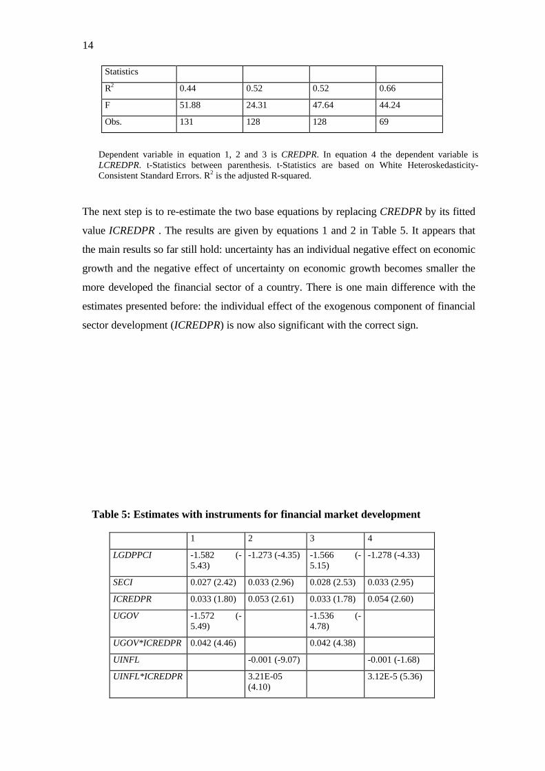
Table 9: Different samples of countries. Estimates for UINFL

LGDPPCI<7.615 LGDPPCI>7.615 LDC DC

LGDPPCI -1.774 (-2.87) -2.287 (-4.22) -1.506 (-5.07) -2.157 (-4.40)

SECI 0.082 (2.01) 0.026 (2.22) 0.047 (2.84) -0.021 (-1.25)

ICREDPR 0.064 (2.90) 0.042 (1.79) 0.081 (5.18) -0.007 (-0.95)

UINFL -0.0009 (-7.19) -0.002 (-1.55) -0.0009 (-8.44) -0.495 (-1.78)

UINFL*ICREDPR 2.39E-05 (3.81) 2.28E-05 (0.60) 2.16E-05 (2.41) 0.0097 (1.73)

CONSTANT 10.686 (2.68) 18.174 (4.36) 9.006 (4.60) 23.424 (5.57)

Statistics

R2 0.46 0.40 0.44 0.65

F 8.05 6.41 10.74 9.03

Obs. 43 42 62 23


Table 8 and Table 9 show that the main result concerning the effect of financial sector

development on the uncertainty-economic growth relationship holds for the relatively

low-income groups. Both for the group of countries having a LGDPPCI below the

median value as well as the group of LDCs the individual uncertainty terms are negative

and significant, whereas the interactive terms are positive and significant. The results for

the more developed income groups are somewhat mixed. In some cases the main result

still holds. This is, for instance, the case for effects of UGOV on countries having a

LGDPPCI above the median value. In other cases, the uncertainty term as well as the

20

interactive term becomes insignificant. The reason might be that for richer countries the

specification of the model is not appropriate. It may also be the case that the sample

becomes too small to get reliable results. This especially holds for the estimates in which

the sample consists of only the group of developed countries

Finally, I test whether the coefficients for the variables of interest (in our case, the

coefficients for the uncertainty measure and the interaction term) are robust when some

additional variables are taken into account in the base regressions. The analysis starts by

defining a group of variables that are usually found to be important in growth regressions.

From this group additional variables to be included in the regressions are drawn. I use the

following set of variables:

an indicator for ethnic diversity (ETHFRAC); the number of assassinations per million

inhabitants (ASSASSINATION); the black market premium (LBMP); the number of

coups (COUPS); the longitude (LONGITUDE); an index of political rights (PRIGHTS);

an indicator for trade openness (TRADE); tax receipts divided by GDP (TAX); the

number of revolutions (REVOLUTION); an indicator for perception of corruption

(GRAFT); the value of government consumption as a percentage of GDP (GOV) and the

inflation rate (INFL).

Next, I determine all possible combinations of three of the above-presented set of 12

variables and perform regressions in which the base variables are included as well as 3

additional variables. This implies that, for all base models, 12!/(9!3!) = 220 variants

(models j) are estimated. Per regression 9 independent variables are taken into account

(the constant, LGDPPC, SECI, ICREDPR,UGOV or UINFL, the interaction term, and 3

additional variables from the pool of 12).

I start by conducting an extreme bound analysis (EBA) in line with Levine and Renelt

(1992). The procedure is as follows. For each regression j an estimate for the coefficient

and the standard error of the variable under concern is obtained. The lower extreme

bound is the lowest value of the coefficient minus two times the standard error. The upper

bound is the highest value of the coefficient plus two times the standard error. If the signs

of the upper and lower extreme bounds differ, the variable is not robust according to the

EBA analysis. The extreme bounds are given in Table 10 in the columns High and Low.

21

According to this sensitivity test, UGOV and the interaction term between UGOV and

ICREDPR are robust. Inflation uncertainty and the interaction term between inflation

uncertainty and financial market development are not robust.

The EBA analysis is criticized for being too strict a robustness test. If only in one of the

220 regressions the variable under concern is not significant, the test concludes that the

variable is not robust. Therefore, I also perform a stability analysis in line with Sala-i-

Martin (1997a). The stability test entails to looking at the distribution of these

coefficients, and calculating the fraction of the cumulative distribution function lying on

each side of zero. By assuming that the distribution of the estimates of the coefficients is

normal and calculating the mean and the standard deviation of this distribution, the

cumulative distribution function (CDF) can be calculated.

More precisely, if βj is the coefficient for the variable in variant (model) j, and σj is the

standard error of the coefficient βj, I proxy the mean and the standard deviation of the

distribution by:

n

= jβ

βΣ

n

= jσ

σΣ

where n =220.

In Table 10, the mean estimate is given by the column Average Coefficient. The mean

standard deviation by the column Average Standard Error.

Table 10: Robustness test

Average

Coefficient

AverageStandardError

High Low CDF AverageR2

Robust1 Robust2

Results for equation containing UGOV

ICREDPR 0.024 0.017 0.065 -0.019 0.924 0.51 No No

22

UGOV -1.589 0.302 -0.611 -2.728 1 0.51 Yes Yes

UGOV*ICREDPR 0.043 0.010 0.085 0.011 1 0.51 Yes Yes

Results for equation containing UINFL

ICREDPR 0.048 0.020 0.097 -0.005 0.993 0.38 No Yes

UINFL -0.141 0.077 0.442 -1.047 0.963 0.38 No Yes

UINFL*ICREDPR 0.005 0.003 0.041 -0.022 0.955 0.38 No Yes

Average coefficient: the average coefficient of all equations estimated; Average Standard Error: the averagestandard error of all equations estimated. High (low) is the highest (lowest) coefficient from the entire group ofestimates (calculated as coefficient plus or minus 2 times the standard error). CDF: cumulative distributionfunction. Average R2: the average adjusted R-squared for al equations estimated. Robust1: robust accordingto EBA analysis; Robust2: robust according to the robustness test of Sala-i-Martin. For both sets of estimates220 equations are estimated.

By using a table for the (cumulative) normal distribution, I am able to calculate which

fraction of the cumulative distribution function is on the right or left-hand side of zero.

The test statistic I use is defined as the mean over the standard deviation of the

distribution. In Table 10 CDF denotes the larger of the two areas. If CDF is above 0.95, I

conclude that the variable under consideration has a robust effect on economic growth. It

appears that both inflation uncertainty and uncertainty with respect to government

expenditures have a robust negative effect on economic growth. Most importantly, for

both variables the interaction term has a robust positive effect on economic growth. This

once again suggests that the policy uncertainty-economic growth relationship is

dependent on the development of the financial sector. The results with respect to the

individual term for financial sector development are mixed. The model testing inflation

uncertainty suggests that financial sector development has an individually robust and

positive effect on economic growth. However, the model testing the effects of uncertainty

with respect to government expenditures concludes the opposite.

As explained in Section 4, it is possible to calculate a threshold value of the financial

development indicator above which policy uncertainty starts to have a positive effect on

economic growth. This can be done by dividing the coefficient for the interactive term by

the absolute value of the coefficient for the individual uncertainty variable. For instance,

if the estimates presented in Section 5 with respect to UGOV are considered (Table 5

equation 1), it can be easily calculated that the threshold value of ICREDPR equals about

37% (1.572/0.042). It should be noted that the outcome of this exercise should not be

23

taken too literally since confidence intervals for the variables are not taken into account.

Since the estimate of the threshold is based on two coefficients it is somewhat arbitrary to

calculate a confidence interval. The highest value of the threshold could be obtained by

dividing the coefficient for the interactive term plus two times the corresponding standard

error by the coefficient for the individual uncertainty term minus two times the standard

error of this term.10 This would result in an upper value of the threshold of 2.145/0.023 =

92%. The lower extreme is found by dividing the coefficient for the interactive term

minus two times the standard error by the coefficient for the individual term plus two

times the standard error. This would result in a lower extreme of 0.999/0.061 = 16%.

Since this interval is very large, it is a dangerous exercise to determine the set of countries

for which a rise in policy uncertainty will probably have a positive effect on economic

growth. The more important result of this paper is that it strongly suggests that countries

with a more developed financial sector are better able to undo negative policy uncertainty

effects than countries with a poorly developed financial sector.

7. CONCLUSIONS

In this paper, I examine whether financial sector development may partly undo growth-

reducing effects of policy uncertainty. By performing a standard cross-country growth

regression for the 1970-1998 period I show that policy uncertainty has a robust and

negative individual effect on per capita economic growth. More importantly, I find some

strong evidence that countries with a more developed financial sector are better able to

nullify the negative effects of policy uncertainty on per capita economic growth.

The results of this paper point at two important policy conclusions. First, especially for

developing countries where the financial sector is often very rudimentary, a stable and

credible government policy appears to be of utmost importance. Second, a well-

developed financial sector is an important means by which growth reducing effects of

policy uncertainties can be undone. This clearly indicates the relevance of financial sector

development.

10 Standard errors are calculated by dividing the coefficient by the t-value.

24

Appendix1: List of Variables and sources

ASSASSINATION = The average number of assassinations per million inhabitants for the

1970-1993 period. Source: Easterly and Yu (1999). Original source:Banks Cross national

time-series data archive.

BMP = the average black market premium (%) for the 1970-1997 period. Source:

Easterly and Yu (1999).

COUPS = The average number of coups for the 1970-1988 period. Source: Easterly and

Yu (1999). Original source Banks Cross national time-series data archive.

CREDPR = The average value of credit to the private sector as a percentage of GDP for

the 1970-1997 period. Source: World Bank (1999)

DC = Developed countries.

ETHFRAC = Indicator for ethnic diversity. Source: Easterly and Yu (1999).

GOV = The average value of government consumption as a percentage of GDP

for the 1970-1997 period. Source: World Bank (1999)

GRO = The average real per capita growth rate over 1970-1998 period . Calculated from

real GDP per capita data in constant dollars. Source: Easterly and Yu (1999). Original

source: Penn World Table 5.6 (Summers-Heston data). Missing data calculated from

1985 GDP per capita and GDP per capita growth rates (Global Development Finance &

World Development Indicators).

ICREDPR = The forecasted value of CREDPR based on an estimate in which CREDPR

is explained by LGDPPCI, LAWRULE, LEGGERMAN and a constant.

INFL = The average inflation rate over the 1970-1998 period. Source: Easterly and Yu

(1999). Original source: Global Development Finance & World Development Indicators.

LBMP = Log (1+BMP)

25

LDC = Developing countries

LGDPPCI = The logarithm of the 1970 value of real GDP per capita in constant dollars

(international prices, base year 1985). Source: Easterly and Yu (1999). Original source:

Penn World Table 5.6.

LCREDPR = The value of credits by financial intermediaries to the private sector divided

by GDP. It excludes credits issued by the monetary authorities and government agencies

(which are included in CREDPR). See Levine, Loayaza and Beck (1999). The data come

from the Levine-Loaza-Beck Data Set (available on internet:

http:/www.worldbank.org/html/prdmg/grthweb/llbdata.html)

LICREDPR = The forecasted value of LCREDPR based on an estimate in which

LCREDPR is explained by LGDPPCI, LAWRULE, LEGGERMAN and a constant.

LONGITUDE = Longitude. Source: Easterly and Yu (1999.

PRIGHTS = Average value of an index of political rights for the 1970-1990 period (from

1 to 7; 1 is most political rights). Source: the Barro-Lee (1994) data set.

REVOLUTION = The average number of revolutions for the 1970-1993 period. : Easterly

and Yu (1999). Original source: Banks Cross national time-series data archive.

SECI = The 1970 secondary school enrollment rate. Source: Easterly and Yu (1999).

Original source: Global Development Finance & World Development Indicators.

TAX = The average value of total tax revenue as a percentage of GDP for the 1970-1997

period. Source: World Bank (1999).

TRADE = The average value of exports plus imports divided by GDP for the 1970-1997

period. Source: World Bank (1999). This variable measures the degree of openness.

26

UGOV = Indicator which measures uncertainty concerning the government consumption

to GDP ratio. It is calculated by taking the standard deviation of the unexplained part.

The expected government consumption is measured by using the ordinary least squares

technique.

UGOV1 = Indicator which measures uncertainty concerning the government consumption

to GDP ratio. It is calculated by taking the standard deviation of the unexplained part.

The expected government consumption is measured by using a GARCH approach.

UGOV2 = Indicator which measures uncertainty concerning the government consumption

to GDP ratio. It is calculated by taking the standard deviation of the original series.

UINFL = Indicator which measures uncertainty concerning the inflation rate. It is

calculated by taking the standard deviation of the unexplained part. Expected inflation is

measured by using the ordinary least squares technique.

UINFL1 = Indicator which measures uncertainty concerning the inflation rate. It is

calculated by taking the standard deviation of the unexplained part. Expected inflation is

measured by using a GARCH approach.

UINFL2 = Indicator which measures uncertainty concerning the inflation rate. It is

calculated by taking the standard deviation of the original series.

GOVERNANCE INDICATORS

The six aggregate governance indicators described below are kindly provided by Pablo

Zoido-Lobaton. See Kaufmann, Kraay and Zoido-Lobaton (1999) for an extensive

description. Governance is measured on a scale of about -2.5 to 2.5 with higher values

corresponding to better outcomes. The data are based on data for 1997 and 1998.

1) GOVEFF = An indicator of the ability of the government to formulate and implement

sound policies. It combines perceptions of the quality of public service provision, the

quality of the bureaucracy, the competence of civil servants. the independence of the civil

27

service from political pressures, and the credibility of the government’s commitment to

policies into a single grouping.

2) GRAFT = This indicator measures perception of corruption: the exercise of public

power for private gain.

3) LAWRULE = Indicator which measures the extent to which agents have confidence in

and abide by the rules of society. These include perceptions of the incidence of both

violent and non-violent crime, the effectiveness and predictability of the judiciary, and the

enforceability of contracts. See Kaufmann, Kraay and Zoido-Lobaton (1999) for an

extensive description. Data obtained from the authors.

4) PINST = This index combines indicators which measure perceptions of the likelihood

that the government in power will be destabilized or overthrown by possibly

unconstitutional and/ or violent means.

5) REGBURDEN= An indicator of the ability of the government to formulate and

implement sound policies. It includes measures of the incidence of market-unfriendly

policies such as price controls or inadequate bank supervision, as well as perceptions of

the burdens imposed by excessive regulation in areas such as foreign trade and business

development.

6) VOICE = This index includes indicators which measure the extent to which citizens of

a country are able to participate in the selection of governments.

LEGAL ORIGIN INDICATORS

The five legal system indicators are obtained from Easterly and Yu (1999). They are

zero-one dummies.

1) LEGBRITISH = National legal system from British origin.

2) LEGFRENCH = National legal system from French origin.

3) LEGGERMAN = National legal system from German origin.

4) LEGSCAN = National legal system from Scandinavian origin.

28

5) LEGSOCIALIST = National legal system from Socialist origin

29

Appendix2: Countries in data set

Countries in the sampleAlgeria Costa Rica Indonesia Netherlands SudanAngola Cote d'Ivoire Ireland New Zealand SwazilandArgentina Denmark Israel Niger SwedenAustralia Dominican

RepublicItaly Nigeria Syrian Arab

RepublicAustria Ecuador Jamaica Norway TanzaniaBelgium Egypt, Arab

Rep.Japan Pakistan Togo

Benin El Salvador Kenya Panama Trinidad andTobago

Bolivia Ethiopia Korea, Rep. Paraguay TunisiaBotswana Finland Lesotho Peru UgandaBrazil France Luxembourg Philippines United KingdomBurkina Faso Gabon Madagascar Poland UruguayBurundi Gambia, The Malaysia Portugal VenezuelaCameroon Ghana Mali Romania ZambiaCanada Greece Malta Rwanda ZimbabweCentral AfricanRepublic

Guatemala Mauritania Saudi Arabia

Chile Guinea Mauritius Senegal

China Guinea-Bissau

Mexico Sierra Leone

Colombia Hong Kong,China

Morocco Singapore

Comoros Iceland Mozambique South Africa

Congo, Dem.Rep.

India Nepal Spain

The base model with UGOV contains the 94 countries shown in the table. Due to taking instruments,the Central African Republic and the Comoros drop out of the sample (no data available forRULELAW). Hence, estimates with UGOV and instruments contain 92 countries. If UINFL isincluded the following countries drop out of the sample: Angola, Benin, Comoros, Guinea, HongKong, Mali, Romania and Swaziland. On the other hand, Taiwan is included in addition to thecountries in the table shown above (no data available for GOV). The group of developed countries(DC) contains: Australia, Austria, Belgium, Canada, Denmark, France, Finland, Greece, Hong Kong,Iceland, Ireland, Israel, Italy, Japan, Luxembourg, Malta, Netherlands, New Zealand, Norway,Portugal, Singapore, Spain, Sweden and the United Kingdom.

31

REFERENCES

Abel, A.B. (1983), “Optimal investment under uncertainty,” American Economic Review,

72, 228-233.

Abel, A.B. and J.C. Eberly (1994), “A unified model of investment under uncertainty,”

American Economic Review, 84, 1369-1384.

Aizenman, J. and N.P. Marion (1993), “Macroeconomic uncertainty and private

investment,” Economics Letters, 41, 207-210.

Arrow, K.J. (1968), “Optimal capital policy with irreversible investment,” in J.N. Wolfe

(ed.), Value, Capital and Growth, Essays in Honour of Sir John Hicks, Edinburgh

University Press.

Barro, R.J. (1991), “Economic growth in a cross-section of countries,” Quarterly

Journal of Economics, 106, 407-443.

Barro, R.J. and J.W. Lee (1994), Data set for a panel of 138 countries, NBER Internet

site, 1994.

Barro, R.J. and X. Sala-i-Martin (1995), Economic Growth, McGraw-Hill, New York.

Bernanke, B.S. (1983), “Irreversibility, uncertainty and cyclical investment,” Quarterly

Journal of Economics, 98, 85-106.

Caballero, R.J. (1991), “On the sign of the investment-uncertainty relationship,”

American Economic Review, 81, 279-288.

Calvo, G. (1988), “Costly trade liberalisations: durable goods and capital mobility,” IMF

Staff Papers, 35, 461-473.

Dixit, A.K. and R.S. Pindyck (1994), Investment under uncertainty, Princeton University

Press.

Easterly, W. and H. Yu (1999), Global Development Network Growth Database,

available on internet:

http://www.worldbank.org/html/prdmg/grthweb/gdndata/htlm.

Ghosal, V. (1991), “Demand uncertainty and the capital-labor ratio: evidence from the

U.S. manufacturing sector,” The Review of Economics and Statistics, 73, 157-160.

Ghosal, V. (1995), “Input choices under price uncertainty,” Economic Inquiry, 142-158.

32

Ghosal, V. and P. Loungani (1997), The differential impact of uncertainty on investment

in small and large businesses, Manuscript.

Greenwald, B. and J. Stiglitz (1990), “Macroeconomic Models with Equity and Credit

Rationing,”in Hubbard, R.G. (ed.), Asymmetric information, Corporate Finance,

and Investment. Chicago: University of Chicago Press, pp. 15-42.

Gurley, J.G. and E.S. Shaw (1955), Money n a theory of finance, Washington, DC: The

Brookings Institution.

Hermes, N. and R. Lensink (Eds.) (1996), Financial development and economic growth:

theory and experiences from developing countries, London: Routledge.

Hermes, N. and R. Lensink (1998), “Financial development and economic growth:

evidence from Latin America,” in Auroi (ed.), Latin American and East European

economies in transition: a comparative view, EADI book series 21, Frank Cass,

London, 61-83.

Kaufmann, D., A. Kraay and P. Zoido-Lobaton (1999), Governance matters, Policy

Research Working Paper no. 2196, World Bank, Washington, D.C.

King, R.G. and R. Levine (1993), “Finance and growth: Schumpeter might be right,”

Quarterly Journal of Economics, 108, 717-737.

Leahy, J. and T.M. Whited (1996), “The effects of uncertainty on investment: some

stylized facts,” Journal of Money, Credit, and Banking, 28, 64-83.

Lensink, R. (1999), “Uncertainty, financial development and economic growth: an

empirical analysis,” SOM Research Report 99 E37,University of Groningen.

Lensink, R., H. Bo and E. Sterken (1999), “Does uncertainty affect economic growth?

An empirical analysis,” Weltwirtschaftliches Archiv, 135, 379-396.

Lensink, R., H. Bo and E. Sterken (2000), Investment, capital market imperfections and

uncertainty: theory and empirical results, Edward Elgar, Cheltenham, UK,

forthcoming.

Levine, R. and D. Renelt (1992), “A sensitivity analysis of cross-country growth

regressions,” American Economic Review, 82, 942-963.

Levine, R. (1997), “Financial development and economic growth: views and agenda,”

Journal of Economic Literature, 35, 688-726.

33

Levine, R (1997a), “Law, finance, and economic growth,” Available on the internet:

http://www.worldbank.org/research/.

Levine, R, N. Loayza and T. Beck (1999), “Financial intermediation and growth:

causality and causes,” Available on the internet:

http://www.worldbank.org/research/.

Lucas, R.E. and E.C. Prescott (1971), “Investment under uncertainty,” Econometrica,

39, 659-681.

Peeters, M. (1997), “Does Demand and Price Uncertainty Affect Belgian and Spanish

Corporate Investment?,” De Nederlandsche Bank Staff Reports, No. 13.

Rodrik, D. (1989), “Credibility of trade reform: a policy maker’s guide,” The World

Economy, 12, 1-16.

Sala-i-Martin (1997a), “I just ran two million regressions,” American Economic Review,

87, 178-183.

Sala-i-Martin (1997b), “I just ran four million regressions,” unpublished manuscript,

Colombia University and Universitat Pompeu Fabra.

Schumpeter, J.A. (1939), Business cycles: a theoretical, historical, and statistical

analysis of the capitalist process, New York: McGraw-Hill.

World Bank (1999), World Development Indicators 1999, available on CD-Rom

CREDIT PAPERS

98/1 Norman Gemmell and Mark McGillivray, “Aid and Tax Instability and theGovernment Budget Constraint in Developing Countries”

98/2 Susana Franco-Rodriguez, Mark McGillivray and Oliver Morrissey, “Aidand the Public Sector in Pakistan: Evidence with Endogenous Aid”

98/3 Norman Gemmell, Tim Lloyd and Marina Mathew, “Dynamic SectoralLinkages and Structural Change in a Developing Economy”

98/4 Andrew McKay, Oliver Morrissey and Charlotte Vaillant, “AggregateExport and Food Crop Supply Response in Tanzania”

98/5 Louise Grenier, Andrew McKay and Oliver Morrissey, “Determinants ofExports and Investment of Manufacturing Firms in Tanzania”

98/6 P.J. Lloyd, “A Generalisation of the Stolper-Samuelson Theorem withDiversified Households: A Tale of Two Matrices”

98/7 P.J. Lloyd, “Globalisation, International Factor Movements and MarketAdjustments”

98/8 Ramesh Durbarry, Norman Gemmell and David Greenaway, “NewEvidence on the Impact of Foreign Aid on Economic Growth”

98/9 Michael Bleaney and David Greenaway, “External Disturbances andMacroeconomic Performance in Sub-Saharan Africa”

98/10 Tim Lloyd, Mark McGillivray, Oliver Morrissey and Robert Osei,“Investigating the Relationship Between Aid and Trade Flows”

98/11 A.K.M. Azhar, R.J.R. Eliott and C.R. Milner, “Analysing Changes in TradePatterns: A New Geometric Approach”

98/12 Oliver Morrissey and Nicodemus Rudaheranwa, “Ugandan Trade Policyand Export Performance in the 1990s”

98/13 Chris Milner, Oliver Morrissey and Nicodemus Rudaheranwa,“Protection, Trade Policy and Transport Costs: Effective Taxation of UgandanExporters”

99/1 Ewen Cummins, “Hey and Orme go to Gara Godo: Household RiskPreferences”

99/2 Louise Grenier, Andrew McKay and Oliver Morrissey, “Competition andBusiness Confidence in Manufacturing Enterprises in Tanzania”

99/3 Robert Lensink and Oliver Morrissey, “Uncertainty of Aid Inflows and theAid-Growth Relationship”

99/4 Michael Bleaney and David Fielding, “Exchange Rate Regimes, Inflationand Output Volatility in Developing Countries”

99/5 Indraneel Dasgupta, “Women’s Employment, Intra-Household Bargainingand Distribution: A Two-Sector Analysis”

99/6 Robert Lensink and Howard White, “Is there an Aid Laffer Curve?”99/7 David Fielding, “Income Inequality and Economic Development: A Structural

Model”99/8 Christophe Muller, “The Spatial Association of Price Indices and Living

Standards”99/9 Christophe Muller, “The Measurement of Poverty with Geographical and

Intertemporal Price Dispersion”

99/10 Henrik Hansen and Finn Tarp, “Aid Effectiveness Disputed”99/11 Christophe Muller, “Censored Quantile Regressions of Poverty in Rwands”99/12 Michael Bleaney, Paul Mizen and Lesedi Senatla, “Portfolio Capital Flows

to Emerging Markets”99/13 Christoph Muller, “The Relative Prevalence of Diseases in a Population if Ill

Persons”00/1 Robert Lensink, “Does Financial Development Mitigate Negative Effects of

Policy Uncertainty on Economic Growth?”

DEPARTMENT OF ECONOMICS DISCUSSION PAPERSIn addition to the CREDIT series of research papers the Department of Economicsproduces a discussion paper series dealing with more general aspects of economics.Below is a list of recent titles published in this series.

98/1 David Fielding, “Social and Economic Determinants of English Voter Choicein the 1997 General Election”

98/2 Darrin L. Baines, Nicola Cooper and David K. Whynes, “GeneralPractitioners’ Views on Current Changes in the UK Health Service”

98/3 Prasanta K. Pattanaik and Yongsheng Xu, “On Ranking Opportunity Setsin Economic Environments”

98/4 David Fielding and Paul Mizen, “Panel Data Evidence on the RelationshipBetween Relative Price Variability and Inflation in Europe”

98/5 John Creedy and Norman Gemmell, “The Built-In Flexibility of Taxation:Some Basic Analytics”

98/6 Walter Bossert, “Opportunity Sets and the Measurement of Information”98/7 Walter Bossert and Hans Peters, “Multi-Attribute Decision-Making in

Individual and Social Choice”98/8 Walter Bossert and Hans Peters, “Minimax Regret and Efficient Bargaining

under Uncertainty”98/9 Michael F. Bleaney and Stephen J. Leybourne, “Real Exchange Rate

Dynamics under the Current Float: A Re-Examination”98/10 Norman Gemmell, Oliver Morrissey and Abuzer Pinar, “Taxation, Fiscal

Illusion and the Demand for Government Expenditures in the UK: A Time-Series Analysis”

98/11 Matt Ayres, “Extensive Games of Imperfect Recall and Mind Perfection”98/12 Walter Bossert, Prasanta K. Pattanaik and Yongsheng Xu, “Choice Under

Complete Uncertainty: Axiomatic Characterizations of Some Decision Rules”98/13 T. A. Lloyd, C. W. Morgan and A. J. Rayner, “Policy Intervention and

Supply Response: the Potato Marketing Board in Retrospect”98/14 Richard Kneller, Michael Bleaney and Norman Gemmell, “Growth, Public

Policy and the Government Budget Constraint: Evidence from OECDCountries”

98/15 Charles Blackorby, Walter Bossert and David Donaldson, “The Value ofLimited Altruism”

98/16 Steven J. Humphrey, “The Common Consequence Effect: Testing a UnifiedExplanation of Recent Mixed Evidence”

98/17 Steven J. Humphrey, “Non-Transitive Choice: Event-Splitting Effects orFraming Effects”

98/18 Richard Disney and Amanda Gosling, “Does It Pay to Work in the PublicSector?”

98/19 Norman Gemmell, Oliver Morrissey and Abuzer Pinar, “Fiscal Illusion andthe Demand for Local Government Expenditures in England and Wales”

98/20 Richard Disney, “Crises in Public Pension Programmes in OECD: What Arethe Reform Options?”

98/21 Gwendolyn C. Morrison, “The Endowment Effect and Expected Utility”

98/22 G.C. Morrisson, A. Neilson and M. Malek, “Improving the Sensitivity of theTime Trade-Off Method: Results of an Experiment Using Chained TTOQuestions”

99/1 Indraneel Dasgupta, “Stochastic Production and the Law of Supply”99/2 Walter Bossert, “Intersection Quasi-Orderings: An Alternative Proof”99/3 Charles Blackorby, Walter Bossert and David Donaldson, “Rationalizable

Variable-Population Choice Functions”99/4 Charles Blackorby, Walter Bossert and David Donaldson, “Functional

Equations and Population Ethics”99/5 Christophe Muller, “A Global Concavity Condition for Decisions with

Several Constraints”99/6 Christophe Muller, “A Separability Condition for the Decentralisation of

Complex Behavioural Models”99/7 Zhihao Yu, “Environmental Protection and Free Trade: Indirect Competition

for Political Influence”99/8 Zhihao Yu, “A Model of Substitution of Non-Tariff Barriers for Tariffs”99/9 Steven J. Humphrey, “Testing a Prescription for the Reduction of Non-

Transitive Choices”99/10 Richard Disney, Andrew Henley and Gary Stears, “Housing Costs, House

Price Shocks and Savings Behaviour Among Older Households in Britain”99/11 Yongsheng Xu, “Non-Discrimination and the Pareto Principle”99/12 Yongsheng Xu, “On Ranking Linear Budget Sets in Terms of Freedom of

Choice”99/13 Michael Bleaney, Stephen J. Leybourne and Paul Mizen, “Mean Reversion

of Real Exchange Rates in High-Inflation Countries”99/14 Chris Milner, Paul Mizen and Eric Pentecost, “A Cross-Country Panel

Analysis of Currency Substitution and Trade”99/15 Steven J. Humphrey, “Are Event-splitting Effects Actually Boundary

Effects?”99/16 Taradas Bandyopadhyay, Indraneel Dasgupta and Prasanta K.

Pattanaik, “On the Equivalence of Some Properties of Stochastic DemandFunctions”

99/17 Indraneel Dasgupta, Subodh Kumar and Prasanta K. Pattanaik,“Consistent Choice and Falsifiability of the Maximization Hypothesis”

99/18 David Fielding and Paul Mizen, “Relative Price Variability and Inflation inEurope”

99/19 Emmanuel Petrakis and Joanna Poyago-Theotoky, “Technology Policy inan Oligopoly with Spillovers and Pollution”

99/20 Indraneel Dasgupta, “Wage Subsidy, Cash Transfer and Individual Welfare ina Cournot Model of the Household”

99/21 Walter Bossert and Hans Peters, “Efficient Solutions to BargainingProblems with Uncertain Disagreement Points”

99/22 Yongsheng Xu, “Measuring the Standard of Living – An AxiomaticApproach”

99/23 Yongsheng Xu, “No-Envy and Equality of Economic Opportunity”

99/24 M. Conyon, S. Girma, S. Thompson and P. Wright, “The Impact ofMergers and Acquisitions on Profits and Employee Remuneration in the UnitedKingdom”

99/25 Robert Breunig and Indraneel Dasgupta, “Towards an Explanation of theCash-Out Puzzle in the US Food Stamps Program”

99/26 John Creedy and Norman Gemmell, “The Built-In Flexibility ofConsumption Taxes”

99/27 Richard Disney, “Declining Public Pensions in an Era of DemographicAgeing: Will Private Provision Fill the Gap?”

99/28 Indraneel Dasgupta, “Welfare Analysis in a Cournot Game with a PublicGood”

99/29 Taradas Bandyopadhyay, Indraneel Dasgupta and Prasanta K.Pattanaik, “A Stochastic Generalization of the Revealed Preference Approachto the Theory of Consumers’ Behavior”

99/30 Charles Blackorby, WalterBossert and David Donaldson, “Utilitarianismand the Theory of Justice”

99/31 Mariam Camarero and Javier Ordóñez, “Who is Ruling Europe? EmpiricalEvidence on the German Dominance Hypothesis”

99/32 Christophe Muller, “The Watts’ Poverty Index with Explicit PriceVariability”

99/33 Paul Newbold, Tony Rayner, Christine Ennew and Emanuela Marrocu,“Testing Seasonality and Efficiency in Commodity Futures Markets”

99/34 Paul Newbold, Tony Rayner, Christine Ennew and Emanuela Marrocu,“Futures Markets Efficiency: Evidence from Unevenly Spaced Contracts”

99/35 Ciaran O’Neill and Zoe Phillips, “An Application of the Hedonic PricingTechnique to Cigarettes in the United Kingdom”

99/36 Christophe Muller, “The Properties of the Watts’ Poverty Index UnderLognormality”

99/37 Tae-Hwan Kim, Stephen J. Leybourne and Paul Newbold, “SpuriousRejections by Perron Tests in the Presence of a Misplaced or Second BreakUnder the Null”

Members of the Centre

Director

Oliver Morrissey - aid policy, trade and agriculture

Research Fellows (Internal)

Adam Blake – CGE models of low-income countriesMike Bleaney - growth, international macroeconomicsIndraneel Dasgupta – development theoryNorman Gemmell – growth and public sector issuesKen Ingersent - agricultural tradeTim Lloyd – agricultural commodity marketsAndrew McKay - poverty, peasant households, agricultureChris Milner - trade and developmentWyn Morgan - futures markets, commodity marketsOliver Morrissey (Director) – aid policy, trade and agricultureChristophe Muller – poverty, household panel econometricsTony Rayner - agricultural policy and trade

Research Fellows (External)

V.N. Balasubramanyam (University of Lancaster) - trade, multinationalsDavid Fielding (Leicester University) - investment, monetary and fiscal policyGöte Hansson (Lund University) - trade and developmentMark McGillivray (RMIT University) - aid and growth, human developmentJay Menon (ADB, Manila) - trade and exchange ratesDoug Nelson (Tulane University) - political economy of tradeDavid Sapsford (University of Lancaster) - commodity pricesHoward White (IDS) - macroeconomic impact of aid, povertyRobert Lensink (University of Groningen) – macroeconomics, capital flowsScott McDonald (Sheffield University) – CGE modellingFinn Tarp (University of Copenhagen) – macroeconomics, CGE modelling

Does Financial Development Mitigate Negative Effects of ...

Documents

Transcript of Does Financial Development Mitigate Negative Effects of ...