1

Does exporting increase productivity? Evidence from India

Megha Mukim*

London School of Economics

June 20, 2011

Abstract

This paper identifies two separate effects – that of exporting on productivity across firms, and that of starting to export on productivity within firms. It uses detailed panel data from 1990 to 2008 for over 8,000 manufacturing firms in India across 4-digit product categories. The findings show that exporting is associated with a jump in productivity, both within industries and within firms, but that this effect tapers over time. Entry into export markets has a positive effect on firm performance in the very beginning, but there is no evidence of sustained learning-by-exporting.

JEL Classification: F14, D24 Keywords: Exporting, Productivity, Within Firms versus Across Firms, India

* Department of International Development, London School of Economics, Email: m.mukim@lse.ac.uk; Website: http://personal.lse.ac.uk/mukim. I am grateful to Diana Weinhold, TN Srinivasan and James Harrigan for helpful comments and suggestions, to David Weinstein, Amit Khandelwal and other participants at the Trade Colloquium at Columbia University, to Ana Fernandes, HL Kee and other seminar participants at the World Bank, to Patrick Conway and other participants at the Rocky Mountain Empirical Trade Conference, and to Michael Ferrantino and other participants at the US International Trade Commission for useful discussions.

2

1 Introduction In this paper, I examine the link between exporting and productivity for manufacturing firms in India. I study firm-level data in India at the National Industrial Classification (NIC) level for the period 1990-2008. With the exception of the last few years, this period saw significant entry into exports markets – see Figure 1. I find three main results. First, I demonstrate that firms’ productivity is positively related to their participation in export markets, across firms and within firms. Second, I show that part of the increase in productivity is accounted for by learning-by-exporting, after having controlled for any self-selection into exporting. And third, I find that the learning-by-exporting effect is the highest immediately subsequent to entry into exporting and then begins to level off. An important empirical finding of the literature (Roberts and Tybout 1997, Clerides et al 1998, Bernard and Jensen 1999, Van Biesebroeck 2006, Alvarez and Lopez 2005) is that exporters are more productive than non-exporters. There are two mechanisms that can explain this difference - the first is related to self-selection and the second to learning-by-exporting. Exporters may be more productive than their counterparts, who only supply the domestic market, simply because more productive firms are able to engage in export activity and compete in international markets. The second, more important mechanism, and one which this paper will focus on, is learning-by-exporting by firms, in other words, post-entry productivity benefits. The idea being that when firms enter export markets they gain new knowledge and expertise, which allows them to improve their level of efficiency. However, the two effects are not mutually exclusive – it is possible that high productivity firms that enter the export market continue to improve their productivity because of their exposure to exporting. The remainder of the paper is organised as follows: The next section provides a descriptive overview of the theoretical and empirical literature on exporting and firm productivity. Section 3 describes the data and shows that exporters are in fact different from non-exporters in a number of ways. Section 4 outlines the empirical specification for unbiased production function estimates, and the identification of gains from exporting. Section 5 carries out robustness checks and Section 6 concludes.

2 Theory and Evidence The potential link between trade and economic growth has been fundamental to international and to development economics. This paper concerns itself with the question of whether firms achieve higher productivity growth by becoming exporters. The empirical and theoretical literatures have moved forward in fits and starts. Earlier endogenous growth models (Grossman and Helpman 1991, Rivera-Batiz and Romer 1991) predicted that international technology diffusion through exposure to export

3

markets could boost within-plant productivity1. The traditional export-led growth hypothesis (Kaldor 1970, Dixon and Thirlwall 1975) posited that external demand would enable firms to exploit economies of scale2 leading to productivity growth. Firms could also invest in productivity-enhancing technology in anticipation of larger export markets (Yeaple 2005). Another microeconomic channel is the reallocation of economic activity across firms within industries. Models by Helpman and Krugman (1985) and Krugman (1994) predicted that average productivity could rise if resources were shifted to industries with lower average costs. Heterogeneous firm models (Melitz 2003 and Bernard et al 2003) also argue that the existence of trade costs allows only the most productive firms to enter export markets. As low productivity firms exit, output and employment are reallocated towards higher productivity firms and average industry productivity increases. In other words, it is the reallocation of activity across firms, and not within-firm productivity growth, that drives industry-level productivity. A slew of papers test the predictions of these theoretical models, and their empirical findings demonstrate that differences between exporters and non-exporters could arise whether or not exporting enhanced productivity. There are many studies that find little or no evidence of learning-by-exporting. See Table 1 for a summary of some key studies. For instance Bernard and Jensen (1999) find that the benefits from exporting for American firms are unclear. Although employment, growth and profitability are higher for exporters, productivity and wage growth is not superior. Kim (2000) finds only marginal increases in productivity following trade liberalisation in Korea. Delgado et al (2002) find evidence of higher productivity for exporters versus non-exporters, and evidence of self-selection of more productive firms into the export market. However, they do not find much evidence to support the learning-by-doing hypothesis, and if so, only for younger exporters. Castellani (2002) finds evidence of productivity gains associated with increases in export intensity. Other studies, such as Isgut (2001) and Clerides et al (1998), the latter using data from several countries, also conclude in favour of the self-selection and against the learning-by-exporting hypothesis. Only the most productive firms have a sufficient cost advantage to overcome transportation costs and compete internationally. Exporters are more productive than non-exporters, not because there are any benefits associated with export activities, but they are simply more productive from the outset. Some studies look at trade liberalisation in general and not just exporting. Hung et al (2004) find that exporting activity itself does not seem to promote productivity in the US, and that it is import competition that attributed for the largest part of labour productivity growth in manufacturing during 1996-2001. Pavcnik (2002) and Fernandes (2007) find that it is trade liberalisation more generally that has a strong positive impact on firm-level 1 Industrial-level productivity could also rise if individual firms’ new technological learning spill over and positively affect the total stock of knowledge for all firms, thus raising aggregate productivity. 2 Firms move to a lower point on the average cost curve since a rise in output is accompanied by a less than proportionate rise in average costs.

4

productivity in Chile and Columbia, respectively. Indeed the former is one of the few papers in the literature that is able to identify the within-industry and the within-plant effects. However, some studies do find empirical support for post-entry productivity gains. For instance, Kraay (1999) for China, Bigsten et al (2004) for sub-Saharan Africa, and Aw et al (2000) for Taiwan, find evidence of learning-by-exporting. Loecker (2007) finds that Slovenian export entrants become more productive once they start exporting, and that the productivity gap between exporters and their domestic counterparts widens over time. He also finds that productivity gains are higher for firms exporting to higher-income regions. Biesebroek (2005) finds evidence that sub-Saharan exporters are more productive than their counterparts who only serve the domestic market, and that the former enjoy increasing rates of productivity growth. Other examples of some studies are Castellani (2002), Baldwin and Gu (2003, 2004), Blalock and Gertler (2004), Girma et al. (2004) and Greenaway and Kneller (2008). Park et al (2010) study firms in China and find that the productivity gains are greater for firms that export to more developed markets. However, not all studies are able to describe the source of these learning effects. A notable exception is Baldwin and Gu (2004). From their analysis of Canadian plants they conclude that exporters learn from participation in export markets through channels that include new innovations, as well as technology transfer from abroad and investments in absorptive capacity such as human capital. A recent working paper by Tabrizy and Trofimenko (2010) studies the effect of exporting on productivity for firms in India. They find no evidence of post-entry productivity gains and conclude that productivity differences between exporters and non-exporters are explained only by self-selection. There are some crucial differences between this paper and their study. Although the sample of firms comes from the same data source, their period of study covers only a ten-year period (1998-2008) whilst this paper studies firms over a twenty-year period (1989-2008). Additionally their measure of productivity, which has been calculated using Levinsohn-Petrin techniques, controls for simultaneity bias but does not control for endogenous exit. As capital-intensive firms are better able to weather a negative productivity shock and thus more likely to survive in the market, and since exporters also tend to be more capital-intensive than non-exporters, this suggests that their productivity estimate does not account for the large downward bias on the capital coefficient. They also deflate firm-level data using a national wholesale price index and not industry-specific input and output deflators. Most importantly, their paper describes pre- and post-entry productivity differentials between exporters and non-exporters mainly by using dummy variables for different types of exporting behaviour. It is interesting that for the same countries different studies (albeit, not always for overlapping periods in time) find confirming or conflicting evidence of learning-by-exporting effects. For instance, both papers that study the United States (Bernard and Jensen 1999, and Hung et al 2004) find no evidence of learning-by-exporting. There are three studies for Germany, of which the first finds a positive result (Bernard and Wagner 1997), while the later two (Wagner 2002, and Arnold and Hussinger 2004) find no effect. Both studies for the United Kingdom (Girma et al 1004 and Greenaway and Kneller

5

2008) find positive effects. For Columbia, the first two studies (Clerides et al 1998 and Isgut 2001) find no evidence, while a later study (Fernandes 2007) finds some evidence. It seems that if a study focuses on a developed country or if it uses cross sectional analysis, it is less likely to find learning-by-exporting effects. It is also possible that firms in developing countries that are further away from the technological frontier and that export to other, perhaps more developed markets, also make larger strides in productivity increases. According to the Global Economic Prospects report (World Bank 2008), progress in developing countries reflects the absorption of pre-existing technologies and not at-the-frontier inventions. The technology achievement index3 for developing countries clearly shows that India is a laggard with a score of 0.04 – the highest value is 0.25 for the United States. Thus, one might expect Indian exporters to enjoy large productivity increases as compared their other domestic counterparts, whilst US exporters may not be much more productive than non-exporters.

3 Data and preliminary analysis 3.1. Data description Firm-level data on output and inputs is drawn from the Prowess database. Prowess is a corporate database that contains normalised data built on a sound understanding of disclosures of over 20,000 companies in India. The database provides financial statements, ratio analysis, fund flows, product profiles, returns and risks on the stock market etc. The Centre for Monitoring of the Indian Economy (CMIE), which collects data from 1989 onwards, assembles the Prowess database. The database contains information on 23,168 firms in agriculture, mining, manufacturing and services for the years 1989 – 2008, yielding a total of 437,283 observations. On average there are 8 years of data on each firm. However, data are either not available or are reported as missing values for a number of observations for different variables such as sales, capital stock and wages. This paper focuses mainly on firms in the manufacturing sector, since their exporting behaviour is more easily observable. After cleaning the data4, the final dataset contains 8,253 firms for the years 1989-2008, yielding a total of 69,286 observations. There is a large degree of firm heterogeneity in terms of size and age. Firms in the sample also include both exporters and non-exporters – a total of 5,191 firms enter the export

3 The technology achievement index is published by the United Nations Development Programme and combines (a) the indicators of human skills (mean years of schooling in the population age 15 and older and enrollment ratio for tertiary-level science programs); (b) the diffusion of old innovations (electricity consumption per capita and telephones per capita) and of recent innovations (Internet hosts per capita and high- and medium-tech exports as a share of all exports); and (c) the creation of technology (patents granted to residents per capita and receipts of royalties and license fees from abroad). The index is constructed as simple averages of these indicators within subgroups and then across groups. 4 I exclude observations for which data on sales, gross assets and wages are missing. I check whether these values are systematically missing for particular industries, years or types of firm (by age, and by type of ownership), and find that this is not the case.

6

market at least once over the period of study. Some caveats should be mentioned here. It is not mandatory for firms to supply data to the CMIE, and one cannot tell exactly how representative of the industry is the membership of the firms in the organisation. Prowess covers 60-70 percent of the organised sector in India, 75 percent of corporate taxes and 95 percent of excise duties collected by the Government of India (Goldberg et al 20105). Large firms, which account for a large percentage of industrial production and foreign trade, are usually members of the CMIE and are more likely to be included in the database. This also explains why more than 60% of the firms in the sample enter the export market at some point over their lifetime. And so, the analysis is based on a sample of firms that is, in all probability, taken disproportionately from the higher end of the size distribution. As Tybout and Westbrook (1994) point out, a lot of productivity growth comes from larger plants, and so a more comprehensive study might have found smaller average residual effects. 3.2 Preliminary Analysis: Are exporters different? At the outset I am interested in knowing whether the facts found in the literature – that exporters differ from non-exporters – also hold for firms in India. By regressing firm characteristics on a dummy for whether the firm exports, a number of studies have documented that exporters differ from non-exporters in important ways. Following Bernard and Jensen (1999) and others, I first run the following OLS regression that tells me whether firms that export are different from those that don’t:

€

ln xit = α + βEXPit + γControlsit + δ tTimet + λkIndkk∑ + ξ jDistrict j

j∑ +ε ikt

t∑ (1)

where

€

x refers to the characteristics of firm

€

i at period

€

t active in industry

€

k in district

€

j ,

€

EXP is an export dummy equal to one when the firm is an exporter and zero otherwise. Firm-specific controls include the size (number of employees), the age and the type of firm (private domestic, private foreign, public or mixed). I also control for industry, year and location effects, where subscripts

€

k ,

€

t and

€

j run through the number of industries

€

(Ind), years

€

(Time), and districts (

€

District ) respectively. The coefficient

€

β reveals to what extent exporters differ from non-exporters, within the same year, industry and district. The results are presented in column (1) of Table 3. However, this regression doesn’t say anything about whether there is something about the act of exporting that makes exporters different from non-exporters. Indeed, if I re-run regression (1), comparing exporters with non-exporters before the former started to export, I find that exporters were different from the outset – see column (2) of Table 3. Thus, to know if exporting is truly associated with any changes in firm characteristics, I run the following OLS regression that tells me whether participation in export markets is associated with differential characteristics for a given firm:

€

ln xit = α + βEXPit + γControlsit + δ iFirmi + δ tTimett∑ +ε it

i∑ (2)

5 Quoted in earlier version of NBER working paper.

7

where

€

x refers to the characteristics of firm

€

i at time

€

t active in any particular industry and location.

€

EXP is an export dummy equal to one when the firm exports and zero otherwise. Firm-specific controls include the size and the age of the firm. The difference is that since I am now mainly interested in within-firm variation with regards to exporting over time, I include firm and year fixed effects. The coefficient

€

β reveals whether a given firm is different with regard to exporting. The results are reported in column (3) of Table 3. The results show that exporters are indeed different from non-exporters: they have a higher wage bill (128 per cent higher), operate on a larger scale, add higher value, sell more and invest more than non-exporters. However, this is not very informative in itself because exporters were different from the outset. Thus, what is pertinent is that, for a given firm, participation in export markets is associated with a higher wage bill (57 per cent higher), more assets, more value added, higher sales and more investment. While others in this field have compared exporters to non-exporters within a given industry, location and/or year and found differences (see Table 1), the data for firms in India clearly shows that these differences could easily be driven by intrinsic pre-exporting differences. And that only by studying firm characteristics for a given firm can one truly identify the association, if any, between the act of exporting and productivity. It should be kept in mind that nominal values are deflated using NIC 2-digit level output and input specific price indices. Since more productive forms are likely to have a lower-than-average firm specific price, the use of industry price indices might systematically underestimate the output of more productive firms and therefore underestimate their productivity. On the other hand, if exporters were more likely to use better quality inputs and materials, then using industry-specific deflators would overestimate productivity. The converse would be true for less productive firms. In the absence of firm-specific prices I am unable to overcome this bias. The strong positive association between a given firm’s characteristics and its participation in export markets could reflect the decision of better firms to self select into the export market and/or it could reflect the effect of exporting on the firm. Ultimately I am interested in the effect of exporting on productivity - as Paul Krugman said ‘Productivity isn’t everything, but in the long run it is almost everything’6. The next chapter will deal with the computation of productivity and will then go on to disentangling the effect of exporting on productivity by controlling for the self-selection effect, across firms and within firms.

6 Paul Krugman (1994) The Age of Diminished Expectations, MIT Press.

8

4 Empirical Specification Following the influential papers of Bernard and Jensen (1999) and Clerides et al (1998), the literature has used two main methods to measure learning-by-exporting effects. The first method consists of separating the sample into mutually exclusive groups, such as exporters and non-exporters, to assess differences in plant performance between these groups (see Loecker 2007, Greenaway and Kneller 2008, Girma el al 2004). The second method of measurement of learning-by-exporting effects consists of one or more dummies for lagged export participation in a regression explaining some measure of firm performance. For example, Clerides et al (1998) regress average variable costs on lagged export participation controlling for real exchange rate, lagged capital stock and lagged average variable costs. Kraay (1999) regresses three alternative measures of performance (labour productivity, TFP, and unit costs) on lagged export participation, lagged performance and firm fixed effects. Bigsten et al (2004) and Van Biesebroeck (2004) estimate production functions with a lagged export participation dummy added as a shifter of total factor productivity. The measure of plant performance used in this paper to assess the presence of learning-by-exporting effects is total factor productivity (TFP)7. I use the two-step approach to estimate the causal effect of exporting on firm-level productivity.

4.1 Estimating Productivity The estimation of production functions can be affected by two different sources of bias. Since firms’ inputs and outputs are simultaneously chosen, inputs will be correlated with any shocks, say demand or productivity shocks, that would be captured in the error term and co-efficient estimates will be biased. Under fairly general assumptions8, Levinsohn and Petrin (2003) show that under simple OLS estimations the labour co-efficient will be upward biased and the capital co-efficient will be downward biased, implying that productivity estimates will be upward biased for more capital-intensive firms (such as exporters). On the other hand, the selection problem is generated by the relationship between the unobserved productivity variable and the shutdown decision. In this case, firms’ choices on whether to exit the export market depend on their productivity. Olley and Pakes (1996) obtain consistent production function estimates controlling for the fact that firms’ choices on whether to exit the market depends on their productivity9.

7 TFP measures the economic and technical efficiency with which resources are converted into products. 8 Levinsohn and Petrin (2003) consider the bias in three different cases: when only labour responds to the shock and capital is not correlated with labour (the labour co-efficient will be biased upwards, and the capital co-efficient will be unbiased); when only labour responds to the shock and capital and labour are positively correlated (the labour co-efficient will be biased upwards, and the capital co-efficient will be biased downwards); when labour and capital respond to the shock, the two are positively correlated and labour responds more strongly to the shock (the labour co-efficient will be biased upwards and the capital co-efficient will be biased downwards). 9 Olley and Pakes (1996) use investment as a proxy to control for the simultaneity problem, i.e. when inputs are endogenous to productivity.

9

This paper follows Olley and Pakes (1996) – henceforth referred to as OP – to obtain consistent production function estimates. The OP approach uses investment to control for the simultaneity between inputs and outputs. Consider the following production function:

€

Yit = AitLitβ l Iit

β i Kitβ k

where

€

Yit is output,

€

Ait is total factor productivity, and

€

Lit ,Kit ,Iit represent labour, capital and investment, respectively. TFP is modelled as:

€

Ait = exp(ω it +ε it ) where

€

ω it is a firm-specific productivity shock known to the firm manager, but unknown to the econometrician, and

€

ε it is a zero-mean productivity shock realised after variable inputs have been chosen. The production function of a given firm is described as follows, where output is expressed as a function of the log of inputs and shocks:

€

yit = β0 + βl lit + βkkit + βiiit +ω it +ε it (3) As mentioned above, there is a possibility that the coefficients on the variable input, i.e. labour, are upwardly biased and that there is a corresponding downward bias in the coefficient on the quasi-fixed input, i.e. capital. To obtain consistent production function estimates, I use the OP procedure. Estimation proceeds in two stages. In the first stage, I obtain the coefficients on labour by semi-parametric techniques. It is assumed that a firm’s demand for investment increases monotonically with productivity, conditional on capital. Then the inverse of the investment demand function depends only on observable inputs and capital, and its non-parametric estimate can be used to control for unobservable productivity, removing the simultaneity bias. Since productivity is assumed to affect capital with a lag10, there is no simultaneity problem in estimation the coefficient on capital. Loecker (2010) argues that if firms that export are also firms that invest more, then using the OP procedure would overestimate the capital coefficient and underestimate the returns from exporting. I do not include past exporting experience when estimating productivity, although I do carry out a robustness check by including lagged exports as a state variable later in the paper. The OP procedure also controls for the endogeneity of firm exit by computing survival probabilities for the firm. The probability that the firm survives in the market depends on lagged values of capital and the proxy for productivity. These probabilities control for the selection bias and are based on some threshold of productivity below which a firm exits the market. The survival probabilities are then introduced into the production function to generate the coefficient on capital. In Appendix A, I discuss the estimation algorithm for

10 More specifically, it is assumed that productivity follows a Markov process:

€

ω it = E[ω it |ω it−1]+ ξit where

€

ξit represents the unexpected part of current productivity to which capital does not adjust.

10

getting reliable estimates of the production function in more detail. Nominal values have been deflated using output (sales) and input (labour, capital, investment) deflators11. I re-run Equations (1) and (2) with the computed measure of unbiased productivity as the dependent variable. I find that exporters are 11 per cent more productive than non-exporters. More importantly, I find that for a given firm, exporting is associated with a 26 per cent increase in productivity. I also run Equation (2), i.e. with firm and year fixed effects by 2-digit National Industrial Classification (NIC) and find that the positive association between exporting and productivity is broadly positive across firms in all manufacturing industries, with the exception of tobacco products – see Table 5. Another way to see this relationship is graphically. I rescale time in such a way so that

€

t =1 refers to the year when the firm begins to export,

€

t = 2 is when the firm has exported for a year and so on and so forth. The relationship between productivity and exporting for a given firm is shown in Figure 3. The bold lines refer to the estimated coefficient for the dummy variable that equals 1 if the firm exports, after controlling for firm characteristics (size and age) and including firm and year fixed-effects. The dashed lines show the 99% confidence intervals around the parameter estimates. The levels of TFP jump at the time of entry into export markets and then taper off and do not grow over time. I emphasise here that these regressions do not control for endogenous self-selection of more productive firms into exports, but they do find that (1) exporters are different from non-exporters within the same industry, location and year, and that (2) for a given firm, exporting is associated with a jump in productivity. 4.2 Identification of productivity gains from exporting In the following sub-sections I will identify two separate estimates of exporting on productivity, using propensity score matching and instrumental variables techniques. The first estimate is a within-industry estimate that provides me with the effect of exporting on aggregate industrial productivity after controlling for the self-selection of more productive firms into the export market. This estimate of productivity is directly comparable with other empirical papers in the literature that also compare productivity differentials between exporters and non-exporters within a given industry (and often within a given location and year). The second estimate is a within-firm estimate that provides me with the effect of entry into export markets on aggregate firm productivity after controlling for the self-selection problem. In other words, I will identify the effect of exporting on a given firm over time and the coefficient would no longer be constrained to be the same across all firms. In summary, this section will separate the cross-section variation across firms using Propensity Score Matching (PSM), and the time-series variation within firms using Instrumental Variables (IV).

11 Where the input deflators are constructed by their weight in the Consumer Price Index basket, and the data is taken from the Central Statistical Organisation.

11

Across-Firm Estimate (Propensity Score Matching) Following Girma et al (2004) and Loecker (2007), I control for the self-selection of more productive firms in a given industry into export markets (i.e. the Melitz effect) by creating control groups using matching techniques based on average treatment models as suggested by Heckman et al (1997). The aim of this methodology is to evaluate the causal effect of exporting on productivity by matching export starters with non-exporters. The identifying assumption in estimating the treatment effect (i.e. exporting) comes from the introduction of the state variable – lagged productivity – in the matching procedure and this has a strong interpretation in the underlying structural framework. The method constructs a counterfactual that allows me to analyse how productivity of a firm would have evolved if it had not started exporting. The main problem in this type of analysis is that one does not observe the counterfactual and therefore it is necessary to match the exporting firm with a control group of similar firms that do not export. The aim is to evaluate the causal effect of exporting on the performance indicator – here, TFP. Following Loecker (2007) I rescale the time periods in such a way that a firm starts exporting at

€

s = 0. Let

€

ω is be the outcome at time

€

s - the productivity of firm

€

i at period

€

s - following entry in export markets at

€

s = 0 and the variable

€

STARTi takes on the value one if the firm

€

i starts to export. The causal effect can be verified by looking at the difference: (

€

ω is1 −ω is

0), where the superscript denotes the export behaviour. The crucial problem is that

€

ω is0 is not observable. I follow the micro-econometric evaluation literature

(Heckman et al 1997) and I defined the average effect of export entry on productivity as:

€

E[ω is1 −ω is

0 | STARTi =1] = E[ω is1 | STARTi =1] − E[ω is

0 | STARTi =1] (4) The key difficulty is to identify a counterfactual for the last term in Equation (4). This is the productivity effect that entrants in export markets would have experienced, on average, had they not exported. What is mainly of interest is the magnitude of the ‘impact’, labelled in red in Figure   4 and the main problem is the calculation of the counterfactual that is to be deducted from the total change. This counterfactual is estimated by the corresponding average value of firms that remain non-exporters:

€

E[ω iso | STARTi = 0]. An important feature of the construction of the

counterfactual is the selection of a valid control group. In order to identify this group it is assumed that all the differences in productivity (except that caused by exporting) between exporters and the appropriately selected control group is captured by a vector of observables, including the pre-export productivity of a firm. The intuition behind selecting the appropriate control group is to find a group that is as close as possible to the exporting firm in terms of its predicted probability to start exporting. More formally, I apply the propensity score matching method as proposed by Rosenbaum and Rubin (1983). This boils down to estimating a probit model with a dependent variable equal to one if a firm starts exporting and zero elsewhere on lagged observables including productivity.

12

The probability of starting to export is modelled as follows.

€

START is a dummy variable that equals one at the time a firm starts exporting. The probability of starting to export, i.e. the propensity score, can be represented as follows:

€

Pr(STARTi,0 =1) = F(ω i,−1,CONTROLSi,−1) (5) where

€

F(.) is the normal cumulative distribution function. The re-scaling of the time periods implies that the probability of starting to export is regressed on variables prior to this period

€

s = 0 and I use the subscript ‘

€

−1’ to denote this. The most important variable in estimating the propensity score estimation clearly is the productivity variable. Differences in productivity will be conditioned on pre-export levels of productivity and the size and age of the firm. I also include a full set of industry and year dummies to control for common aggregated demand and supply shocks. I use nearest-neighbour one-to-one matching, with replacement12. Let the predicted export probability for firm

€

i (which is an eventual exporter) be denoted by

€

pi . The matching is based on the method of the nearest neighbour, which selects a non-exporting firm

€

j that has a propensity score

€

p j closest to that of the export entrant. This results in a group of matched exporting and non-exporting firms needed in order to evaluate the causal impact of exporting on productivity. Following both Girma et al (2004) and Loecker (2007) I match within each 2-digit NIC sector and therefore create control groups within narrowly defined sectors as opposed to matching across the entire set of firms. This is likely to be important as the marginal effect of various variables on the probability of starting to export may differ substantially between different sectors due to different technological and market conditions that firms face in different industries. This implies that I estimate the probability to start exporting for each industry separately, allowing the coefficients to vary across the various industries. However, I am unable to control for other differences between firms that produce the same product, for instance, quality, mark-ups, employee skill sets etc. Once I have this counterfactual in hand I use a difference-in-differences (DID) methodology to assess the impact of exporting on productivity. Following Loecker (2007) the estimator of the learning-by-exporting effect (

€

βLBE ) is calculated in the following way. Assume

€

N firms that started exporting and a set

€

C of control firms and

€

ω1 and

€

ω c are the estimated productivity of the treated and the controls respectively. Denote

€

C(i) as the set of control units matched to a firm

€

i with a propensity score of

€

pi . The number of control firms that are matched with an observation

€

i (starter) is denoted as

€

Nic and the weight

€

wij =1Ni

c if

€

j ∈C(i) and zero otherwise. In this way every firm

€

i that

started exporting is matched with

€

Nic control firms. I stress that the matching is always

performed at the time a firm starts exporting and

€

s = {1,2,.....,S} denotes the time periods after the decision to start exporting, i.e. at

€

s = 0. I introduce two estimators getting at the

12 Matching with replacement tends to reduce bias, and can be performed in cases where the control group is smaller than the treatment group.

13

productivity effect at every time

€

s (Equation 8) and a cumulative productivity effect (Equation 9). The estimator

€

βLBEs at every period

€

s after the decision to start exporting is given by:

€

βLBEs =

1Ns i∑ ω is

1 − wijω jsc

j∈C (i)∑ )

⎛

⎝ ⎜ ⎜

⎞

⎠ ⎟ ⎟ (6)

In words, I estimate the productivity premium of firms that started exporting at each period

€

s compared with (a weighted average of) productivity of a control group based on nearest neighbour matching at every period

€

s. However, since I am also interested in how starting to export impacts the productivity trajectory of a firm, I estimate the average cumulative treatment effect. This is the productivity gain gathered over a period

€

S after the decision to start exporting. The estimator

€

βLBES is given by:

€

βLBES =

1NS

ω is1 − wijω js

c

j∈C ( i)∑

s=0

S

∑s=0

S

∑⎛

⎝ ⎜ ⎜

⎞

⎠ ⎟ ⎟

i∑ (7)

This provides me with an average cumulative productivity gain at every time period and plotting these estimated coefficients over time gives me a relation between time (

€

s) and the productivity gain. The estimate in Equation (9) gives us the productivity premium new exporters have gathered over time. This implies that the entire productivity path of export entrants is compared to that of the control group, whereas the estimate in Equation (8) estimates the productivity premium at the each time period

€

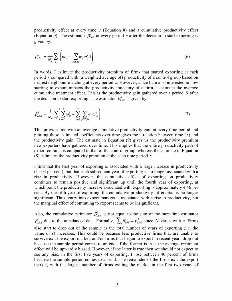
s. I find that the first year of exporting is associated with a large increase in productivity (11.03 per cent), but that each subsequent year of exporting is no longer associated with a rise in productivity. However, the cumulative effect of exporting on productivity continues to remain positive and significant up until the fourth year of exporting, at which point the productivity increase associated with exporting is approximately 4.46 per cent. By the fifth year of exporting, the cumulative productivity differential is no longer significant. Thus, entry into export markets is associated with a rise in productivity, but the marginal effect of continuing to export seems to be insignificant. Also, the cumulative estimator

€

βLBES is not equal to the sum of the pure time estimator

€

βLBEs due to the unbalanced data. Formally,

€

βLBEs

s∑ ≠ βLBE

S since

€

N varies with

€

s. Firms also start to drop out of the sample as the total number of years of exporting (i.e. the value of s) increases. This could be because less productive firms that are unable to survive exit the export market, and/or firms that began to export in recent years drop out because the sample period comes to an end. If the former is true, the average treatment effect will be upwardly biased. However, if the latter is true then we should not expect to see any bias. In the first five years of exporting, I lose between 40 percent of firms because the sample period comes to an end. The remainder of the firms exit the export market, with the largest number of firms exiting the market in the first two years of

14

exporting. And so, the coefficients could be biased upwards since I am unable to control for endogenous exit. The propensity matching score method also assumes that there exists a region of ‘common support’, where the treated and control propensity scores overlap, and over which a robust comparison can be made. A straightforward way to check overlap is a visual analysis of the density distribution of the propensity scores across the treated and control groups before and after matching (see Figure 5). Firms that fall outside of the region of common support are disregarded and for these firms the treatment effect cannot be estimated. With matching the proportion of such firms is small, and since the region of common support is vastly improved the estimated effect on the remaining firms can be viewed as representative. In Table 7 I provide the t-test of the equality of means between the treated and the matched control group. I find that there is no statistically significant difference in the means of the conditioning variables between the treated and the control group, and that matching reduces the bias by 19 percent for productivity to 95 percent for sales.

Within-Firm Estimate (Instrumental Variables) The problem with propensity score matching techniques is that it eliminates the selection problem based only on observables, and that it assumes away every possible problem with the error terms – this could include endogeneity and/or measurement error. Additionally, this estimate only provides me with the productivity differential between exporters and non-exporters within a given industry, and says nothing about the within-firm effect of exporting on productivity. In this section, I will use an instrument to deal with the methodological shortcomings of the matching procedure, and to identify that part of the effect of exporting on productivity that is owing to time-series variation. A good instrument would be a variable that affects the productivity of the firm only through its effect on the firm’s decision to export, and which would be exogenous to changes in firm-level productivity. I use effectively applied tariffs faced by exporting firms. These tariffs are defined by destination country for each industrial sector at the NIC 4-digit level from 1990 to 2008. Since these are tariffs imposed by destination countries, individual firms in India should not be able to affect the level of tariffs. And in theory, a fall in tariffs should positively affect a firm’s decision to enter the export market and thus affect firm-level productivity. One might argue that increases in firm-level productivity in India could have a direct impact on tariffs faced by exporting firms if destination markets raised their tariffs to protect their domestic markets. If this were the case, one would expect to see a positive relationship between exporting and tariffs. But in fact tariffs and exports are negatively related (see Figure 6), and so it would seem more likely that lower tariffs drive higher export volumes. Alternatively one may argue that an increase in firm-level productivity leads to an increase in exports, which in turn creates pressure from exporting firms from the originating country, i.e. India, on destination markets to lower their tariffs. In other

15

words, that exports are driving tariffs. However, India’s share of the global export market is tiny, and since independence has varied between 0.5 and 2.5 percent and between 0.5 and just over 1 percent over the period of study. When disaggregated by sector the range varies between 0.32 and 0.55 percent. When further disaggregated by the top 20 country destinations (that make up almost 75 percent of the total market share of Indian exports), the range varies between 5.72 and 0.09 percent (see Figure 9). So, a more likely story would be that Indian exporters are in fact price takers in global markets13. It has been argued that India is able to punch above its weight at the WTO, for instance through anti-dumping investigations. In fact in 2002, India overtook the US to become the highest initiator of anti-dumping cases at the WTO. However, the point of anti-dumping cases is mainly to try and protect domestic markets from cheap imports. For instance, most anti-dumping cases were brought out against China, Brazil, and Taiwan etc. It could, however, be the case that countries may still use anti-dumping as a clever negotiating tool to increase market access. I use effectively applied tariff rates, in levels and changes, taken from the Trade Analysis and Information System (TRAINS)14. The classification system used is ISIC Revision 3 as this corresponds on a one-to-one basis to the Indian NIC system. I re-run Equation (1) with productivity as the dependent variable and I instrument the dummy variable for starting to export with tariffs, weighted by exports. My instrument, i.e. tariffs, varies by industry and year, whilst my instrumented variable, i.e. the dummy variable for when the firm starts exporting, varies by firms over time. I am unable to find an instrument that is specific to firms, but I use tariffs at the 4-digit industry level to narrow the effect as best I can. As in my earlier OLS specifications, I include firm fixed-effects, which also controls for the differential effects that changes in industry-level tariffs would have on firms depending on their individual characteristics. I also include year fixed-effects. Thus, the instrument is time varying and applies within firms. Recall, that productivity here has been calculated after having controlled for the potential simultaneity of input choices and unobserved exit, and so I am mainly trying to control for any reverse causality between productivity and the decision of the firm to start exporting. I run the regression using changes and levels of weighted tariffs, using two-stage least squares techniques. I check the exogeneity of the export status using the Durbin-Wu Hausman specification test, and find that the results of the IV estimates are preferable. The instrumented coefficient remains positive and significant. The F-statistic is above the rule-of-thumb value of 10 in the case of changes in tariffs, but this is not the case for tariff levels. I also find that instrumenting for starting to export raises the coefficient dramatically. With OLS techniques starting to export is associated with a 15.88 percent increase in productivity. However, instrumenting with changes in tariffs raises this effect to 24.71 percent. Similarly, when instrumenting with tariff levels the co-efficient rises to 84.17 13 It could be argued that Indian exporters may be able to influence tariffs in products where they have a small share of the destination market precisely because the latter might not care about providing better access, especially if in return it were able to gain concessions in other sectors. 14 TRAINS data is made available through the World Integrated Trade Solution (WITS) database.

16

percent, although the coefficient is not statistically significant. My endogenous variable, exports, is weakly correlated with my instruments, whether changes or levels of tariffs (see Table 8 for first-stage results). In general, the weaker the correlation between the instrument and the variable being instrumented, the greater is the population variance of the coefficient. The increase in the instrumented coefficient could also be owing to heterogeneity in export effects, implying that the marginal return to exporting is higher for lower productivity firms, who are also more affected by changes in effectively applied tariffs. Biesebroeck (2005) finds a similar result using ethnicity of the owner as an instrument, and Card (2001) elaborates on such econometric results when using instrumental variables.

5 Robustness and Other Exercises 5.1 Intensive Margin Another interesting sub-question is whether productivity is determined not just by participation in export markets, but also by the intensity of that participation. In other words, firm productivity could be affected by the extensive margin of exporting (i.e. participation), but additionally it could be affected by the intensive margin of exporting wherein firms increase their years and/or intensity of exports. As pointed out by Park et al (2010) one might expect to see continued improvements in productivity with more years of exporting if for instance, productivity-enhancing investments are lumpy and firms make additional investments following a few years of exporting. Research by Blalock and Gertler (2004) and Kraay (1999) finds that firms grow more productive with continued participation in export markets. Others, such as Castellani (2002) and Girma et al (2004) find that export intensity is also related to larger increases in firm-level productivity. In this section, I examine how productivity changes are related to continued participation (and discontinuation of that participation) and the intensity of that participation in export markets. First, I examine within the same regression, how entry into, continued stay in and exit from export markets impacts firm-level productivity. I follow Bernard and Jensen (1999) and run the following modified regression:

€

(ω iT −ω i0)T

= β0 + β1startiT + β2stopiT + β3continueiT + γControlsiT + δ iFirmi +ε iTi∑

(8) where

€

startiT =1 if a firm did not export at 0 but exports at

€

T ,

€

stopiT =1 if a firm exported at 0 but no longer at

€

T and

€

continue1iT =1 if a firm exports at both

€

T and 0, interacted with the number of years of exporting up to 5 years, and

€

continue2iT =1 is interacted with the number of years of exporting up to 10 years. Firm-specific controls include the size (number of employees) and the age of the firm. In contrast to other

17

papers that study between-firm effects, since I am mainly interested in within-firm changes, I include firm fixed-effects. According to the results (see Table 10), the year of entry into the export market is associated with an increase in productivity for the firm. Column (1) studies the change in productivity between the year of entry into export markets and the previous year. Column (2) compares the change in productivity between the year of entry into export markets and all subsequent years. In other words, starting to export is associated with an 8.05 per cent increase in productivity from one year to the next, and a 10.45 per cent increase in productivity compared to all subsequent years before entry. However, the positive effect disappears if the firm ‘continues’ to export. The variable ‘continue’ is interacted with the number of years of exporting in the short (5 years) and in the medium term (10 years)15. Although the cumulative change in productivity in the short and medium term in always positive, the effect of exporting begins to taper off in the short terms and the marginal effect is negative in the medium term. Although after 10 years of exporting, firms remain 0.99 per cent more productive than before. What is interesting is that exiting the export market has a negative effect on firm productivity. In the immediate year of exit, the fall in productivity is 18.57 percent, and compared to previous years, the fall in productivity is 11.32 percent. It should be kept in mind that although the OP method controls for endogenous exit from the sample, it does not control for endogenous exit from export markets. And so the negative coefficient on ‘stop’ could be an overestimate since I am unable to observe firms that exit both, the export market and the sample, at the same instant. In the second exercise, following Castellani (2002) and Girma et al (2004) I regress firms’ TFP on exports as a proportion of sales, controlling for the age and size of the firm and with the inclusion of firm fixed-effects (see Column 3). I find that the value of total exports has a positive and significant effect on firms’ productivity – implying that the more that a firm exports, the higher the productivity of the firm. In this case, a percentage point increase in export volume leads to a 4.72 percent in productivity for my sample of firms. 5.2 Spillovers The sample also provides me with information on whether firms belong to particular ownership groups. These are large business groups that own a number of firms, usually operating in similar industries, along the vertical or horizontal scale of production. There are a total of 583 business groups where the mean number of firms within each group is 6.5, the minimum 2 and the maximum 12716. As an example, take the ‘Rane Group’, which has 12 firms that produce steering systems, engine valves, brake linings etc. In any given year, anywhere between 1 to 5 firms within the Rane Group export.

15 The possible range is (1,20), with firms exporting for an average of 4-5 years. 16 The business group with the most firms is the Tata Group.

18

One might expect knowledge spillovers to be high for firms within the same business group since there would be fewer or no restrictions on technology sharing. Technological spillovers are one of the channels through which firms with access to foreign markets became more productive. It could be theorised that non-exporting firms might be able to access better technologies or production processes or designs if other firms within the same business group had access to foreign markets through exporting. I regress productivity of non-exporters in a given business group on the total number of exporting firms within the same business group in that year, controlling for the location, age and size (number of employees) of firms and again I include firm and year fixed-effects since I mainly interested in the effect for a given firm. I also carry out this exercise at the 2-digit NIC level to study how spillovers might matter between firms in industries with higher technological relatedness. I find that on average (see Table 11), the number of exporters within a business group seems to have no statistically significant effect on the productivity of non-exporters within the same business group. I find similar results if I use lagged values. However, when I drill down to particular industry groups I find more interesting results. For manufacturers of rubber and plastic products (NIC 25), the productivity of a given non-exporter falls by 5.92 percentage points if an additional firm within the same business group exports, suggesting that firms within the same business group grow at the expense of others. On the other hand, the effect of additional exporters on the productivity of non-exporters in a given business group is positive for motor manufacturers and for fabricated metal procurers – the productivity of a given non-exporter increases by a whopping 6.69 and 19.84 percent if an additional firm within the same business group exports.

6 Concluding remarks This paper analyses the effect of exporting on firm-level productivity over a period that saw a large increase in the number of exporting firms. Descriptive statistics find that exporting is positively associated with size, capital intensity and value addition, within and across firms. Ultimately, however, what is really interesting is the causal effect of exporting on a given firm’s performance. In the paper I identify the effect of entering export markets after controlling for the self-selection of more productive firms into such markets. Since I am mainly interested in the within-firm effect of exporting, wherever possible, I use firm-fixed effects. This is in stark contrast to the earlier literature that studies between-firm effects. To identify the within-industry effect of exporting on productivity, I use propensity-matching techniques. I construct a set of ‘control firms’ and then evaluate the effect of the ‘treatment’, i.e. exporting. I find that exporting does indeed lead to a positive and significant effect on the productivity of firms that begin to export. I also find that the marginal effect of continuing to export is insignificant, although the cumulative effect of exporting after a few years of exporting is still positive. Since I match firms within a

19

given industry, this methodology allows me to identify the within-industry effect of exporting. Using matching, I control for a Melitz-type effect wherein more productive firms are also more likely to become exporters. I then move on to identifying the effect of exporting on a given firm, i.e. the within-firm productivity premium. I use effectively applied tariffs faced by a given firm in world markets to control for reverse causality. The decision of the firm to enter the export market is instrumented with simple and weighted tariffs – the intuition being that a fall in tariffs would reduce the fixed cost of entry for firms at the margin. Again, I find that entry is associated with a large increase in productivity. The large jumps in productivity immediately subsequent to entry leads me to suspect that firms in my sample might anticipate entry into export markets, making productivity-enhancing investments which then allow them to recoup large productivity premiums in the first few years of exporting. There is no evidence of continued learning-by-exporting effects, whether within-industry or within-firms. I also study the effect of the intensive margin of exporting for firms, for continued participation and for higher intensity of participation. I find that the gains from exporting are the highest in the first few year of entry and then begin to taper off. In other words, after tracking firm performance for up to 5 years, I find that there is no evidence of further productivity benefits, except in those firms that are most exposed to export markets. I also find evidence that productivity gains are reversed when the firm decides to exit the export market. I check for any evidence of spillovers from exporting to non-exporting firms within the same business group, and find that there be positive externalities for some industries, but that on average there are little or no spillovers. My results for the within-industry effects are in line with previous findings in the literature. Loecker (2007) uses propensity-score matching techniques to identify the effect of exporting on firms in Slovenia and finds that the annual productivity premium from exporting varies between 8 to 13 per cent. Using similar techniques, this paper finds that average productivity premium for firms that start to export are 11 per cent, but that these premiums are no longer significant over time. Biesenbroeck (2005) incorporates lagged exports within the production function and finds robust evidence for a positive effect of exporting on productivity. He also uses the ethnicity of the firm owner as an instrument for the decision of firms to export, and again finds evidence for a causal and positive impact. Using different techniques, his estimate of the effect of exporting on productivity varies between 25 to 28 per cent for firms in Africa. I use effectively applied tariffs as instruments, but the instrument applied within-firms and not across-firms, and my estimate of the effect of starting to export is around 24 percent. In other words, I find that the effect of exporting on within-firm productivity is much higher than that for within-industries. This study makes a few contributions to an already crowded literature. It is an attempt to understand the productivity premium from exporting for a poor, rapidly developing country. There has been no previous robust methodological work on answering the age-old, yet classic, question of the effect of exporting on firm-level productivity for a large

20

and increasingly important country like India. Developing countries that are growing briskly are also where one would expect the gains to be the highest. Evidence on the determinants and computation of firm-level productivity in low-income countries is also rare. I also use an instrument, i.e. effectively applied tariffs that has previously not been used in the literature to control for the self-selection effect within firms. The use of tariffs nicely isolates the effect of entry into export markets on productivity, and since these tariffs are hardly unique to the case of India, they could easily be applied in other settings. And lastly and most importantly, to my knowledge, this is a first attempt to identify the effect of participation in export markets that separates the across-firm effect from the within-firm effect. The existing empirical literature focuses almost primarily on controlling for the self-selection of more productive firms within a given industry. In contrast, in this paper I identify the effect of starting to export within firms. Although the question of whether exporting raises aggregate industrial productivity is a tremendously interesting one, it seems perilous to ignore the effects on aggregate firm productivity.

References Alvarez, R. and Lopez, R.A. (2005), ‘Exporting and performance: evidence from Chilean

plants’, Canadian Journal of Economics, 3(4): 1384-1400. Arnold, J. and Hussinger, K. (2004), ‘Export behaviour and firm productivity in German

manufacturing: A firm-level analysis’, Discussion Paper No. 04-12, Centre for European Economic Research (ZEW).

Aw, BY., Chung, S and Roberts, MJ. (2000) ‘Productivity and turnover in the export market: micro-level evidence from the Republic of Korea and Taiwan (China)’, World Bank Economic Review, 14(1): 65– 90.

Baldwin, JR. and Gu, W. (2003), ‘Export market participation and productivity performance in Canadian manufacturing’, Canadian Journal of Economics, 36(3): 634–657.

Baldwin, J.R. and Gu, W. (2004), ‘Trade liberalisation: Export-market participation, productivity growth and innovation’, Oxford Review of Economic Policy, 20(3): 372–392.

Bernard, A. and Jensen, J.B. (1995), ‘Exporters, jobs and wages in US manufacturing: 1976–1987’, Brookings papers on economic activity, Microeconomics, 67–119.

Bernard, A. and Jensen, J.B. (1999), ‘Exceptional exporter performance: cause, effect or both?’ Journal of International Economics, 47: 1-25.

Bernard, A., Eaton, J., Jensen, J.B., and Kortum, S.S. (2003), ‘Plants and productivity in international trade’, American Economic Review, 93(4): 1268-1290

Bernard, A. and Jensen, J.B. (2004), ‘Why some firms export’, Review of Economics and Statistics, 86(2): 561–569.

21

Bernard, A., Jensen, J.B., Redding, S. and Schott, P.K. (2007), ‘Firms in international trade’, NBER Working Paper No. 13054.

Biesebroeck, V.J. (2005), ‘Exporting raises productivity in sub-Saharan African manufacturing firms’, Journal of International Economics, 67: 373-391.

Bigsten, A., Collier, P., Dercon, S., Fafchamps, M., Gauthier, B., Gunning, J.W., Oduro, A., Oostendorp, R., Pattillo, C., Soderbom, M., Teal, F. and Zeufack, A. (2004), ‘Do African manufacturing firms learn from exporting’, Journal of Development Studies, 40 (3): 115– 141.

Blalock, G. and Gertler, P.J. (2004), ‘Learning from exporting revisited in less developed setting’, Journal of Development Economics, 75(2): 397–416.

Blundell, S. and Bond, S. (1998), ‘Initial conditions and moment restrictions in dynamic panel data models’, Journal of Econometrics, 87: 29-52.

Card, D. (2001), ‘Estimating the return to schooling: progress on some persistent econometric problems’, Econometrica, 69(5): 1127–1160.

Castellani, D. (2002), ‘Export behaviour and productivity growth: Evidence from Italian manufacturing firms’, Weltwirtschaftliches Archiv, 138: 605–628.

Clerides, S., Lach, S. and Tybout, J. (1998), ‘Is learning by exporting important? Micro-dynamic evidence from Colombia, Mexico, and Morocco’, Quarterly Journal of Economics, 113(11): 903-947.

Delgado, M.A., Farinas, J.C. and Ruano, S. (2002), ‘Firm productivity and export markets: a non-parametric approach’, Journal of International Economics, 57: 397-422.

Dixon, R.J. and Thirlwall, A.P. (1975), ‘A model of regional growth differences on Kaldorian lines’, Oxford Economic Papers, 27: 201-214.

Fernandes, A.M. (2007), ‘Trade policy, trade volumes and plant-level productivity in Colombian manufacturing industries’ Journal of international economics, 71: 52-71.

Girma, S., Greenaway, D. and Kneller, R. (2004), ‘Does exporting increase productivity? A microeconometric analysis of matched firms’, Review of International Economics, 12(5): 855–866.

Goh, A.T. (2000), ‘Opportunity cost, trade policies and the efficiency of firms’ Journal of Development Economics, 62(2): 363-383.

Goldberg, P, Khandelwal, A., Pavcnik, N. and Topalova, P. (2010), ‘Multiproduct firms and product turnover in the developing world: Evidence from India’, Review of Economics and Statistics, 92(4): 1042-1049.

Greenaway, D. and Kneller, R. (2008), ‘Exporting, productivity and agglomeration’, European Economic Review, 52(5): 919-939.

Grossman, G. amd Helpman. E. (1991), Innovation and Growth in the World Economy, MIT Press: Cambridge.

Heckman, J., Ichimura, H., Smith, J., and Todd, P. (1997), ‘Matching as an Econometric Evaluation Estimator: Evidence from Evaluating a Job Training Programme’, Review of Economic Studies, 64:605–654.

Helpman, E. and Krugman P. (1985), Market Structure and Foreign Trade, MIT Press: Cambridge.

Hung, J., Salomon, M. and Sowerby, S. (2004), ‘International trade and US productivity’, Research in International Business and Finance, 18: 1-25.

Isgut, A.E. (2001), ‘What’s different about exporters? Evidence from Colombian

22

manufacturing’, Journal of Development Studies, 37 (5): 57– 82. Kaldor, N. (1970), ‘The case for regional policies’, Scottish Journal of Political

Economy, 17: 337-348. Kim, E. (2000), ‘Trade liberalization and productivity growth in Korean manufacturing

industries: price protection, market power, and scale efficiency’, Journal of Development Economics, 62(1): 55-83.

Kraay, A. (1999), ‘Exports and economic performance: Evidence from a panel of Chinese enterprises’, Revue d'Economie du Developpement,1(2): 183-207.

Levinsohn, L. and Petrin, A. (2003), ‘Estimating production functions using inputs to control for unobservables’, Review of Economic Studies, 70(2): 317-341.

Loecker, J.D. (2007), ‘Do exports generate higher productivity? Evidence from Slovenia’, Journal of International Economics, 73: 69-98.

Loecker, J.D. (2010), ‘A note on detecting learning by exporting’, NBER Working Paper 16546.

Melitz, M. (2003), ‘The impact of trade on intra-industry reallocations and aggregate industry productivity’, Econometrica, 71 (6): 1695-1725.

Olley, G.S. and Pakes, A. (1996), ‘The dynamics of productivity in the telecommunications equipment industry’, Econometrica, 64 (6): 1263-1297.

Park, A., Yang, D., Shi, X. and Jiang, Y. (2010) ‘Exporting and firm performance: Chinese exporters and the Asian financial crises’, Review of Economics and Statistics, 92(4): 822-842.

Pavcnik, N. (2002) , ‘Trade liberalisation, exit and productivity improvements: Evidence from Chilean plants’, The Review of Economic Studies, 61(1): 245-276.

Rivera-Batiz, L. and Romer, P. (1991), Economic integration and endogenous growth, Quarterly Journal of Economics, 106: 531-555.

Roberts, M. and Tybout, J. (1997), ‘The decision to export in Colombia: An empirical model of entry with sunk costs’, American Economic Review, 87(4): 545–564.

Srinivasan, T.N. And Archana, V. (2009), ‘India in the global and regional trade: determinants of aggregate and bilateral trade flows and firms’ decision to export’, Working Paper No. 232, Indian Council for Research on International Economic Relations (ICRIER).

Tabrizy, S.S. and Trofimenko, N. (2010), ‘Scope for export-led growth in a large emerging economy: Is India learning by exporting?”, Kiel Working Paper No. 1633, Kiel, Germany.

Tybout, J.R. and Westbrook, M.D. (1994), ‘Trade liberalisation and the dimensions of efficiency change in Mexican manufacturing industries’, Journal of International Economics, 39: 53-78.

Wagner, J. (2002), ‘The causal effects of exports on firm size and productivity: First evidence from a matching approach’, Economics Letters, 77: 287–292.

World Bank (2008), ‘Global Economic Prospects: Technology diffusion in the developing world’, Washington DC.

Yasar, M., Raciborski, R. and Poi, B. (2008), ‘Production function estimation in Stata using the Olley and Pakes method’, The Stata Journal, 8(2): 221-231.

Yeaple, S.R. (2005) ‘A simple model of firm heterogeneity, international trade, and wages’, Journal of International Economics, 65: 1-20.

23

Appendix A

A.1 Estimating Productivity

Following Olley and Pakes (1996) it is assumed that in year

€

t the manager observes the firm’s current productivity

€

ω it before choosing labour

€

lt and investment

€

it to combine with the quasi-fixed input, capital

€

kt for the production of output

€

yt . Output is expressed as follows:

€

yt = β0 + βl lt + βiit + βkkt +ω t +ε t (A1)

Inputs are divided into a freely variable ones (

€

lt ,it ) and the state variable capital (

€

kt ). The error term is assumed to be additively separable in a transmitted component (

€

ω t ) and an i.i.d. component (

€

ε t). The key difference between the former and the latter is that the former is a state variable and hence impacts the firm’s decision rules, while the latter has no impact on the firm’s decisions.

Since

€

ω t is known to the manager but unknown to the econometrician and may be positively correlated with

€

lt and

€

it , it generates a potential simultaneity bias that is addressed by the following estimation procedure. The firm’s variable input demands, derived from profit maximisation, depend on privately known productivity and capital. Investment’s demand function is given by:

€

it = i(ω t ,kt ) and it must be monotonic in all

€

ω t for all relevant

€

kt to qualify as a valid proxy – implying that conditional on capital the demand for investment increases with productivity. Assuming that monotonicity holds, the input demand function can be inverted to obtain

€

ω t as a function of investment and capital, as below. Note that this function depends on observables only.

€

ω t =ω(it ,kt )

Consider the problem of self-selection. Firms with larger capital stocks can expect higher returns on capital even in the face of lower levels of productivity, and will choose to stay longer in the market. Thus the self-selection generated by the exit behaviour implies that the expectation of productivity will be decreasing in capital, leading to a negative bias in the capital coefficient.

The first stage of the estimation proceeds by rewriting Equation (A1) in a partially linear form:

€

yt = βl lt + φ(it ,kt ) +ε t (A2) where,

€

φ(it ,kt ) = β0 + βiit + βkkt +ω(it ,kt ) (A3)

24

Since

€

E[ε t | it ,kt ] = 0 , taking the difference between Equation (A2) and its expectation conditional on investment and capital generates the following expression:

€

yt − E[yt | it ,kt ] = βl (lt − E[lt | it ,kt ]+ε t (A4)

Equation (A4) is estimated by OLS (no constant) to obtain consistent parameter estimates for labour. The conditional expectations in Equation (A4) are the intercepts of locally weighted least squares (LWLS) regressions of output and labour on (

€

it ,kt ). After obtaining estimates for

€

βl , we estimate the function

€

φ(.) as a LWLS regression of

€

yt − ˆ β l lt on (

€

it ,kt ). If one were only concerned with the marginal productivities of the variable inputs (but not the co-efficient on the proxy variable) one could stop here. To obtain a capital co-efficient, a plant-level measure of productivity a more complete model for

€

φt (.) will be required since capital enters it twice. To estimate

€

βk , in addition to the estimates of

€

βl obtained from the partially linear model, estimates of the survival probabilities are also used. These probabilities are given by:

€

Pr{χt+1 =1 |ω t+1(kt+1)Jt} ≡ Pt (A5) where

€

χt is defined as the indicator function and is equal to zero if the firm exits the market, and

€

Jt refers to the information available at time

€

t . In the implementation the probability of survival is estimated by fitting a probit model of

€

χt+1 on the state and proxy variables, as well as their squares and cross products.

In the next stage the expectation of

€

yt+1 − βl lt+1 conditional on information at time

€

t and survival is given as:

€

yt+1 − βl lt+1 = βkkt+1 + g(Pt ,φt − βkkk ) + ξt+1 +ε t+1 (A6) where,

€

ξt+1 =ω t+1 − E[ω t+1 |ω t ,χt+1 =1], and is the unexpected productivity shock and is independent and identically distributed (i.i.d.). The unknown function

€

g(.) is approximated by a second-order polynomial in

€

φt − βkkk and

€

Pt17. The estimates of

€

βl ,

€

φt and

€

Pt are substituted in (A6) for the true values of

€

βl ,

€

φt and

€

Pt , to then obtain estimates of

€

βk by minimising the sum of squared residuals in equation (A6). Since the estimation routine involves three steps, the stat command implemented uses the clustered bootstrap errors, treating all observations for a single firm as one cluster.

Following Loecker (2007) with the coefficients of the production function in hand, I then recover a productivity measure for the firm

€

i in industry

€

j at time

€

t 18:

€

ω ijt = yijt −βlj lijt −βkjkijt

17 Readers interested in the details of the estimation system can refer to Yasar et al (2008). 18 It should be noted here that this measure of productivity if not the true unobserved productivity shock. It also includes the i.i.d. component which is assumed to be zero on average.

25

Tables

Table 1: Summary of empirical findings on exports and productivity

Study Country Sample Methodology Evidence*

€

ω e >ω ne

LBE

effects Aw and Hwang (1995) Taiwan 2,832 firms; 1986 Translog production function, cross-section √ x

Bernard and Wagner (1997)

Germany 7,624 firms; 1978-92 Panel Data √ √

Clerides et al (1998) Colombia, Mexico, Morocco

All firms; 1981-91, 1986-90, 1984-91

FIML of cost functions; Panel data √ √1

Kraay (1999) China 2,105 firms; 1988-92 Dynamic panel √ √ Bernard and Jensen (1999)

US 60,000 plants; 1984-92 Linear probability with fixed effects √ x

Kim (2000) Korea 36 sectors; 1966-1988 Translog production function; cross-sections √ x Isgut (2001) Colombia 6453 plants; 1981-1991 Difference-in-Differences methodology (with

dummies) √ x

Delgado et al (2002) Spain 1,766 firms; 1991-96 Nonparametric analysis of productivity distributions

√ x

Castellni (2002) Italy 2,898 firms; 1989-94 Cross-section √ √2 Wagner (2002) Germany 353 firms; 1978-89 Panel data; Matching √ x Alvarez and Lopez (2005)

Chile 5,000 plants; 1990-96 Ordered probit; pooled data √ √

Baldwin and Gu (2003) Canada 8215 firms; 1974-1996; System GMM; Cross-sections √ √

Arnold and Hussinger (2004)

Germany 389 firms; 1992-2000 Olley and Pakes production function; Matching techniques

√ x

Bigsten et al (2004) Cameroon, Ghana, Zimbabwe

289 firms; 1992-1995 Maximum likelihood, System GMM methods; Panel data √ √

Girma et al (2004) UK 8,992 firms; 1988-1999 Matched samples √ √

Hung et al (2004) US 40 industries; 1996-2001 Difference-in-Differences Methodology; Panel data

√ x

Blalock and Gertler (2004)

Indonesia 20,000 firms; 1990-1996 Translog, Olley and Pakes, Levinsohn and Petrin production function;

√ √

Van Bisebroeck (2005) Sub-Saharan Africa

1916 firms (9 countries); 1992-1996

GMM, Maximum likelihood, Olley and Pakes production function; Cross-section √ √

Loecker (2007) Slovenia 7915 firms; 1994-2000 Olley and Pakes production function; Matched samples

√ √

Fernandes (2007) Colombia 6474 plants; 1977-1991 Levinsohn and Petrin for production function; Panel data

√ √

Greenaway and Kneller (2008)

UK 11,225 firms; 1988-2002 Matched samples √ √

Park et al (2010) China 3,339 firms; 1995, 1998, 2000

Instrumental Variables Technique √ √

*

€

ω e >ω ne : Exporters more productive than non-exporters; LBE: Learning-by-exporting effects. 1: Some learning from exporting in the case of Morocco. 2: Learning associated with export intensity. Source: Girma et al (2004), modified and updated

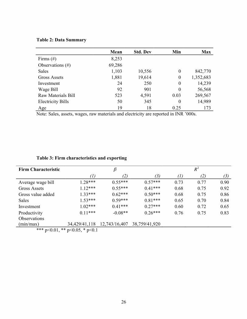
26

Table 2: Data Summary

Mean Std. Dev Min Max Firms (#) 8,253 Observations (#) 69,286 Sales 1,103 10,556 0 842,770 Gross Assets 1,881 19,614 0 1,352,683 Investment 24 250 0 14,239 Wage Bill 92 901 0 56,568 Raw Materials Bill 523 4,591 0.03 269,567 Electricity Bills 50 345 0 14,989 Age 19 18 0.25 173

Note: Sales, assets, wages, raw materials and electricity are reported in INR ’000s.

Table 3: Firm characteristics and exporting

Firm Characteristic

€

β

€

R2 (1) (2) (3) (1) (2) (3)

Average wage bill 1.28*** 0.55*** 0.57*** 0.73 0.77 0.90 Gross Assets 1.12*** 0.55*** 0.41*** 0.68 0.75 0.92 Gross value added 1.33*** 0.62*** 0.50*** 0.68 0.75 0.86 Sales 1.53*** 0.59*** 0.81*** 0.65 0.70 0.84 Investment 1.02*** 0.41*** 0.27*** 0.60 0.72 0.65 Productivity 0.11*** -0.08** 0.26*** 0.76 0.75 0.83 Observations (min/max) 34,429/41,118 12,743/16,407 38,759/41,920

*** p<0.01, ** p<0.05, * p<0.1

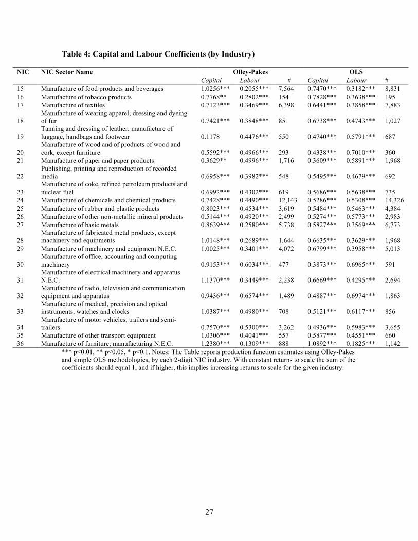
27

Table 4: Capital and Labour Coefficients (by Industry)

NIC NIC Sector Name Olley-Pakes OLS Capital Labour # Capital Labour # 15 Manufacture of food products and beverages 1.0256*** 0.2055*** 7,564 0.7470*** 0.3182*** 8,831 16 Manufacture of tobacco products 0.7768** 0.2802*** 154 0.7828*** 0.3638*** 195 17 Manufacture of textiles 0.7123*** 0.3469*** 6,398 0.6441*** 0.3858*** 7,883

18 Manufacture of wearing apparel; dressing and dyeing of fur 0.7421*** 0.3848*** 851 0.6738*** 0.4743*** 1,027

19 Tanning and dressing of leather; manufacture of luggage, handbags and footwear 0.1178 0.4476*** 550 0.4740*** 0.5791*** 687

20 Manufacture of wood and of products of wood and cork, except furniture 0.5592*** 0.4966*** 293 0.4338*** 0.7010*** 360

21 Manufacture of paper and paper products 0.3629** 0.4996*** 1,716 0.3609*** 0.5891*** 1,968

22 Publishing, printing and reproduction of recorded media 0.6958*** 0.3982*** 548 0.5495*** 0.4679*** 692

23 Manufacture of coke, refined petroleum products and nuclear fuel 0.6992*** 0.4302*** 619 0.5686*** 0.5638*** 735

24 Manufacture of chemicals and chemical products 0.7428*** 0.4490*** 12,143 0.5286*** 0.5308*** 14,326 25 Manufacture of rubber and plastic products 0.8023*** 0.4534*** 3,619 0.5484*** 0.5463*** 4,384 26 Manufacture of other non-metallic mineral products 0.5144*** 0.4920*** 2,499 0.5274*** 0.5773*** 2,983 27 Manufacture of basic metals 0.8639*** 0.2580*** 5,738 0.5827*** 0.3569*** 6,773

28 Manufacture of fabricated metal products, except machinery and equipments 1.0148*** 0.2689*** 1,644 0.6635*** 0.3629*** 1,968

29 Manufacture of machinery and equipment N.E.C. 1.0025*** 0.3401*** 4,072 0.6799*** 0.3958*** 5,013

30 Manufacture of office, accounting and computing machinery 0.9153*** 0.6034*** 477 0.3873*** 0.6965*** 591

31 Manufacture of electrical machinery and apparatus N.E.C. 1.1370*** 0.3449*** 2,238 0.6669*** 0.4295*** 2,694

32 Manufacture of radio, television and communication equipment and apparatus 0.9436*** 0.6574*** 1,489 0.4887*** 0.6974*** 1,863

33 Manufacture of medical, precision and optical instruments, watches and clocks 1.0387*** 0.4980*** 708 0.5121*** 0.6117*** 856

34 Manufacture of motor vehicles, trailers and semi-trailers 0.7570*** 0.5300*** 3,262 0.4936*** 0.5983*** 3,655

35 Manufacture of other transport equipment 1.0306*** 0.4041*** 557 0.5877*** 0.4551*** 660 36 Manufacture of furniture; manufacturing N.E.C. 1.2380*** 0.1309*** 888 1.0892*** 0.1825*** 1,142

*** p<0.01, ** p<0.05, * p<0.1. Notes: The Table reports production function estimates using Olley-Pakes and simple OLS methodologies, by each 2-digit NIC industry. With constant returns to scale the sum of the coefficients should equal 1, and if higher, this implies increasing returns to scale for the given industry.

28

Table 5: Exporting and TFP (by Industry)

NIC NIC Sector Name

€

β Errors #

€

R2 15 Manufacture of food products and beverages 0.2686*** [0.036] 4,955 0.708 16 Manufacture of tobacco products -1.1438*** [0.248] 126 0.789 17 Manufacture of textiles 0.2609*** [0.030] 4,757 0.618 18 Manufacture of wearing apparel; dressing and dyeing of fur 0.6911*** [0.128] 483 0.564 19 Tanning and dressing of leather; manufacture of luggage, handbags and footwear 1.0234*** [0.167] 347 0.701 20 Manufacture of wood and of products of wood and cork, except furniture 0.2577*** [0.093] 228 0.749 21 Manufacture of paper and paper products 0.3966*** [0.058] 1,181 0.560 22 Publishing, printing and reproduction of recorded media 0.1837** [0.072] 373 0.766 23 Manufacture of coke, refined petroleum products and nuclear fuel -0.0323 [0.092] 479 0.619 24 Manufacture of chemicals and chemical products 0.3354*** [0.022] 8,945 0.618 25 Manufacture of rubber and plastic products 0.3084*** [0.040] 2,681 0.635 26 Manufacture of other non-metallic mineral products 0.1969*** [0.043] 2,016 0.557 27 Manufacture of basic metals 0.3733*** [0.040] 3,918 0.628 28 Manufacture of fabricated metal products, except machinery and equipments 0.4486*** [0.062] 1,060 0.705 29 Manufacture of machinery and equipment N.E.C. 0.0813*** [0.028] 3,293 0.716 30 Manufacture of office, accounting and computing machinery -0.1037 [0.152] 320 0.670 31 Manufacture of electrical machinery and apparatus N.E.C. -0.0480 [0.045] 1,713 0.731 32 Manufacture of radio, television and communication equipment and apparatus 0.1458** [0.068] 1,165 0.716 33 Manufacture of medical, precision and optical instruments, watches and clocks 0.1107 [0.094] 469 0.800 34 Manufacture of motor vehicles, trailers and semi-trailers 0.0775*** [0.029] 2,326 0.707 35 Manufacture of other transport equipment 0.1869 [0.116] 475 0.812 36 Manufacture of furniture; manufacturing N.E.C. 0.1914 [0.121] 610 0.568

*** p<0.01, ** p<0.05, * p<0.1. Notes: The Table reports estimates of Equation (2) with the sample restricted to a given 2-digit NIC industry. Each row reports the co-efficient, standard errors clustered at the firm level and the

€

R2 from one regression as well as the number of observations. Table 6: Estimated learning by exporting effects

s 1 2 3 4 5 Outcome: productivity

€

βLBEs 0.1103*** -0.0420 -0.0302 -0.0329 0.0277 [0.038] [0.034] [0.040] [0.039] [0.052]

# treated 4324 3538 3204 2786 2445 # controls 3394 2971 2690 2344 2073 Outcome: cumulative productivity

€

βLBES 0.1103*** 0.0814*** 0.1007*** 0.0446* 0.0072

[0.038] [0.029] [0.029] [0.024] [0.025] # treated 4324 6278 9856 13060 15846 # controls 3394 4558 6322 7484 8022

*** p<0.01, ** p<0.05, * p<0.1 Standard errors in square brackets

29

Table 7: Balancing Tests

Mean t-test Variable Sample Treated Control % bias % bias ↓ t p>|t| Lag (Sales) Unmatched 5.2063 5.6853 -26.6 -10.86 0.000 Matched 5.2063 5.2287 -1.2 95.3 -0.46 0.687 Lag (Productivity) Unmatched -0.1919 -0.3138 9.0 3.88 0.000 Matched -0.1919 -0.0937 -7.2 19.3 -2.27 0.023

Table 8: First-Stage Results

Predictors Start Δ Weighted tariffs -0.0009**

[0.000]

Weighted tariffs (levels) -0.0007* [0.000] Age -0.0052*** -0.0056*** [0.001] [0.001] Size 0.0000 0.0000 [0.000] [0.000]

Firm & Year FE Yes Yes # 16,442 15,899

€

R2 0.496 0.499 Partial

€

R2 0.001 0.001 F-Statistic 10.17 5.61 *** p<0.01, ** p<0.05, * p<0.1

Robust standard errors in square brackets (clustered at the firm level)

30

Table 9: IV Estimation

Predictors OLS IV (Tariffs)

Tariffs (Δ) Tariffs (level) Start 0.1588*** 0.2471* 0.8417 [0.030] [1.036] [2.344] Age -0.0236*** -0.0202 -0.0223*** [0.005] [0.013] [0.008] Size 0.0000 0.0000 0.0000 [0.000] [0.000] [0.000] Firm & Year FE Yes Yes Yes # 16,444 16,442 15,899

€

R2 0.814 0.814 0.815 *** p<0.01, ** p<0.05, * p<0.1

Robust standard errors in square brackets (clustered at the firm level19). The dependent variable is firm-level productivity.

19 The residuals could be correlated across firms or time. For instance, economy-level shocks would cause correlation between firms at a moment in time, and persistent firm-specific shocks could cause correlation across time. Thus, I also cluster standard errors by year, but this does not affect the results.

31

Table 10: Exporting and the Intensive Margin

Variables Δ Productivity Δ Productivity (Cumulative) Productivity

(1) (2) (3) Start 0.0805*** 0.1045* [0.017] [0.013] Continue1 0.0054 0.0124*** (5 years) [0.002] [0.003] Continue2 -0.0038 0.0099*** (10 years) [0.001] [0.002] Stop -0.1857*** -0.1132*** [0.025] [0.026] Log (Exports) 0.0472*** [0.006] Age -0.0004 -0.0002 -0.0003 [0.001] [0.001] [0.000] Size 0.0000 0.0000** 0.0000 [0.000] [0.000] [0.000] Firm & Year FE Yes Yes Yes # 38,440 41,920 25,378

€

R2 0.196 0.829 0.922 *** p<0.01, ** p<0.05, * p<0.1

Robust standard errors in square brackets (clustered at the firm level)

32

Table 11: Business Groups

NIC NIC Sector Name Exporters (sum)

L.Exporters (sum) Observations

15-36 0.0055 2,103 0.770

All 0.0081 1,879 0.792

15 -0.0036 492 0.658

Manufacture of food products and beverages -0.0147 448 0.715

17 -0.0567 146 0.728

Manufacture of textiles -0.0341 124 0.730

21 -0.0278 81 0.746

Manufacture of paper and paper products -0.0104 73 0.742

22 -0.0475 26 0.977

Publishing, printing and reproduction of recorded media -0.0069 22 0.952

23 0.0755 30 0.786

Manufacture of coke, refined petroleum products and nuclear fuel 0.0627 28 0.906

24 0.0271 348 0.688

Manufacture of chemicals and chemical products 0.0190 304 0.653

25 -0.0592*** 93 0.847

Manufacture of rubber and plastic products -0.0778*** 86 0.855

26 -0.0095 188 0.533

Manufacture of other non-metallic mineral products -0.0104 175 0.559

27 0.0053 144 0.643

Manufacture of basic metals 0.0085 128 0.664

28 0.1984*** 29 0.995

Manufacture of fabricated metal products, except machinery and equipments 0.1680*** 25 0.998

29 -0.0235 84 0.852

Manufacture of machinery and equipment N.E.C. -0.0007 74 0.862

30 0.0854 23 0.872

Manufacture of office, accounting and computing machinery 0.0109 18 0.975

31 0.0083 108 0.732

Manufacture of electrical machinery and apparatus N.E.C. 0.0217* 96 0.867

32 -0.0053 52 0.843

Manufacture of radio, television and communication equipment and apparatus 0.0337 48 0.904

34 0.0669*** 116 0.862

Manufacture of motor vehicles, trailers and semi-trailers 0.0504*** 102 0.860

35 -0.0482 52 0.619

Manufacture of other transport equipment 0.0326 46 0.543

*** p<0.01, ** p<0.05, * p<0.1 Robust standard errors clustered at the firm level (not shown)

33

Figures

Figure 1: Number of exporters

Source: Based on Prowess, CMIE (Centre for Monitoring of the Indian Economy)

Figure 2: Technology Achievement Index

Source: Based on data from Global Economic Prospects (World Bank 2008)

34

Figure 3: TFP and entry into export markets

Figure 4: Identification of the true impact

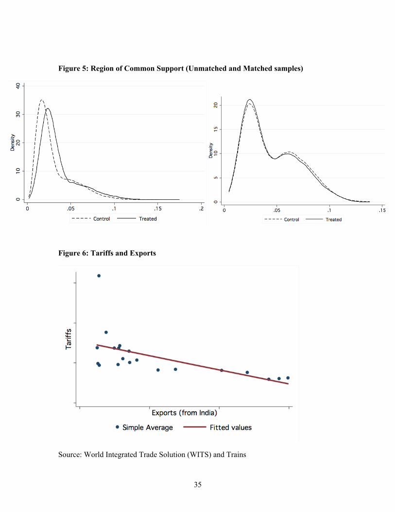
35

Figure 5: Region of Common Support (Unmatched and Matched samples)

Figure 6: Tariffs and Exports

Source: World Integrated Trade Solution (WITS) and Trains

36

Figure 7: Indian Export share

Source: World Integrated Trade Solution (WITS) and Comtrade

Figure 8: Range of export shares by industries

Source: World Integrated Trade Solution (WITS) and Comtrade

37

Figure 9: Range of export shares by top 20 export markets and industries

Source: World Integrated Trade Solution (WITS) and Comtrade