Does Attending a Low-Achieving School Affect High ... Attending a Low-Achieving School Affect...
47
Does Attending a Low-Achieving School Affect High-Performing Student Outcomes? Eric Parsons* February 2015 This paper follows a cohort of initially high-performing Missouri students from grade-3 through grade-9 and examines whether attending a low-achieving school impacts their subsequent standardized exam scores, as well as the grade in which they first take Algebra I. Two key findings emerge. First, attending a low-achieving school does not affect the standardized exam performance of initially high- performing students once school quality (as measured by value-added) is accounted for. Second, high-performing students who attend low-achieving schools are more likely to take Algebra I later relative to their counterparts who attend higher- achieving schools. Keywords: high-performing students, school quality, student achievement, tracking * The author is from the Department of Economics at the University of Missouri. I would like to thank Cory Koedel, Mike Podgursky, Peter Mueser, Bradly Curs, Saku Aura, and Mark Ehlert for their helpful comments on earlier drafts of this manuscript, as well a collaborative relationship with the Missouri Department of Elementary and Secondary Education. The usual disclaimers apply.
Transcript of Does Attending a Low-Achieving School Affect High ... Attending a Low-Achieving School Affect...
Does Attending a Low-Achieving School Affect High-Performing Student Outcomes?
Eric Parsons*
February 2015
This paper follows a cohort of initially high-performing Missouri students from grade-3 through grade-9 and examines whether attending a low-achieving school impacts their subsequent standardized exam scores, as well as the grade in which they first take Algebra I. Two key findings emerge. First, attending a low-achieving school does not affect the standardized exam performance of initially high-performing students once school quality (as measured by value-added) is accounted for. Second, high-performing students who attend low-achieving schools are more likely to take Algebra I later relative to their counterparts who attend higher-achieving schools. Keywords: high-performing students, school quality, student achievement, tracking
* The author is from the Department of Economics at the University of Missouri. I would like to thank Cory Koedel, Mike Podgursky, Peter Mueser, Bradly Curs, Saku Aura, and Mark Ehlert for their helpful comments on earlier drafts of this manuscript, as well a collaborative relationship with the Missouri Department of Elementary and Secondary Education. The usual disclaimers apply.

1
1. Introduction
The topic of ability tracking in K-12 education has received considerable attention in
research (e.g. see Kulik & Kulik, 1982; Oakes, 1985; Gamoran, 1986; Slavin, 1990; Hoffer, 1992;
Argys, Rees, & Brewer, 1996; Betts & Shkolnik, 2000; Figlio & Page, 2002). The argument in favor
of ability tracking is that it reduces the variance of student ability within classrooms, allowing
teachers to more easily target instruction at each student’s individual skill level and increasing
educational efficiency overall (Kerckhoff, 1986; Hallinan, 1994). However, this “technical” view of
tracking is countered by critics who rightly point out that tracking is not simply a production
decision but also has sociological implications, with different tracks conferring differing levels of
social status on the students (Gamoran, 1986). These status effects may combine with poor
instruction in the lower tracks to have significant educational impacts that reinforce and enhance
inequality (Oakes, 1985). Hallinan (1994) provides a nice context for the tracking debate and
ultimately argues for better tracking, not de-tracking.
The literature on tracking in the U.S. has focused largely on within-school tracking in the
secondary grades because, as Hanushek and Woessman (2006) note, “no country tracks students
between differing-ability schools in the early primary grades.” However, to the extent that (a)
housing segregation, school and teacher quality, and other sociological and economic factors result
in variation in average achievement levels across schools (Black, 1999) and (b) instruction at the
school-level is differentiated to account for these differences, students may face de facto tracking from
the moment they enter the public school system. In fact, de facto school-level tracking may be a
larger issue at the elementary level than at the middle and high school levels because elementary
schools are generally less diverse (owing to smaller catchment areas) and do not have formal tracking
policies in place to potentially counter instructional targeting issues.
2
Evidence suggests that differentiated instruction across schools does occur in practice. For
example, Polikoff and Struthers (2013) find that schools serving disadvantaged and advantaged
students have different instructional responses to the accountability pressures imposed by No Child
Left Behind (NCLB), with disadvantaged schools shifting towards activities requiring lower
cognitive demands.1 In addition, low-performing students are more likely to choose to transfer to
the charter sector (Cowen & Winters, 2013), which may be indirect evidence of school-level
instructional targeting. And although social status issues are perhaps less of a concern when de facto
tracking of this nature occurs at the school-level, instructional issues are likely heightened given the
lack of mobility between “tracks.” A notable group of students who may be particularly affected by
this potential misalignment are high-achieving students who attend generally low-achieving schools.
The extent to which this type of de facto school-level tracking is a problem for improperly-tracked
students has not been addressed in previous research.
To better understand if and how high-achieving students are affected by school-level
instructional targeting, this paper follows a cohort of high-achieving students from grade-3 to grade-
9 and examines whether high-achievers are adversely affected by attending generally low-achieving
schools. Two key findings emerge. First, there is no evidence to suggest that attending a low-
achieving school has a negative impact on standardized exam performance for high achievers
through grade-8 (which is typically the end of the standardized testing regime in public K-12
schools). In fact, it appears that schools that are successful at promoting academic growth among
low-achieving students are also doing well with students at the high end of the achievement
distribution. This is in line with much of the larger tracking literature that finds zero to small effects
1 Although NCLB has given way in most states to accountability systems defined by NCLB waivers, recent research suggests that there is a large degree of overlap between the old and new systems (Polikoff, McEachin, Wrabel, & Duque, 2014).

3
of tracking on student achievement (Kulik & Kulik, 1982; Slavin, 1990; Betts & Shkolnik, 2000;
Figlio & Page, 2002).
Second, de facto school-level tracking does appear to affect course-taking outcomes for
high-achieving students in later grades. Specifically, high-achieving students who attend low-
achieving schools take Algebra I later in their schooling careers relative to their high-achieving
counterparts who attend higher-achieving schools. Moreover, these findings for Algebra I may be
indicative of more general challenges in course alignment for these students. Although the test-score
findings suggest that the cognitive development of high-achieving students is not harmed by
attending schools where they differ substantially from their peers, to the extent that delayed course
taking affects college readiness, they may be adversely affected. In fact, these college readiness issues
may provide a partial explanation for why high achievers from disadvantaged backgrounds do not
apply to selective colleges (Hoxby & Avery, in press). The potential negative impacts of course
misalignment are also supported by research suggesting that accelerated coursework has positive
impacts on high-achieving student outcomes (Kulik & Kulik, 1982; Kulik & Kulik, 1984; Burris,
Heubert, & Levin, 2006; Clotfelter, Ladd, & Vigdor, 2012b).
2. Prior Research
The research literature on the effects of tracking in education is long and varied, dating back
at least to the 1930s (Billett, 1932; Whipple, 1936). However, despite the lengthy history of research
on the topic, the state of knowledge on the issue is perhaps best summarized by Betts in his 2011
review of the literature when he states, “What we do not know about the effects of tracking on
outcomes greatly exceeds what we do know.” As mentioned in the introduction, studies examining
the average effects of tracking on student outcomes generally find small to zero effects (Kulik &
Kulik, 1982; Slavin, 1990). However, early studies on the differential effects of tracking generally
find that tracking improves outcomes for high-ability students, while hurting those of low-ability

4
students (Kerckhoff, 1986; Gamoran & Mare, 1989; Hoffer, 1992; Argys, Rees, & Brewer, 1996),
results that support the inequality-enhancing sociological theory of tracking put forth by Oakes
(1985). In a cross-country differences-in-difference analysis, Hanushek and Woessman (2006) also
find that tracking increases inequality, although they find that both low- and high-achieving students
are harmed by tracking with a larger negative effect for low-achieving students.
However, as noted by Betts (2011), methodological issues, endogeneity concerns, and
differing definitions of tracking across districts, states, and nations limit the generalizability of these
results. For example, when Betts and Shkolnik (2000) attempt to control for track selection by
restricting comparisons to similar-ability students in tracked and untracked schools, they find much
smaller differential effects than Hoffer (1992) and Argys, Rees, and Brewer (1996). Figlio and Page
(2002) control for the endogeneity of student placement into tracks by using only school-level
variation (rather than student-type variation) to identify their model and similarly find no effects of
tracking. Furthermore, when the authors also control for the possible endogeneity of school choice,
the differential effects are flipped, i.e. tracking has positive effects for low-achieving students and
negative effects for high-achieving students.
Recent experimental and quasi-experimental studies further add to the variety of estimated
tracking effects. Guyon, Maurin, and McNally (2012) find that a policy change in Northern Ireland
expanding enrollment at elite secondary schools had an overall positive effect on performance, with
a slight negative effect on low-achieving students, a large positive impact on marginal students who
would have attended non-elite schools prior to the policy change but attend elite schools following
the change, and no impact on high-achieving students. In contrast, Duflo, Dupas, and Kremer
(2011) find marked improvements across all ability levels as the result of a tracking experiment in
Kenyan primary schools.

5
In addition to the tracking literature, two other strands of educational research also merit
mention in relation to the present study. The first is the college “mismatch” literature, which
although largely focused on the mechanisms that result in students mismatching to colleges (e.g. see
Roderick, Coca, & Nagaoka, 2011; Bowen, Chingos, & McPherson, 2009; Arcidiacono, Aucejo,
Fang, & Spenner, 2011; Smith, Pender, & Howell, 2013; Dillon & Smith, 2013; Hoxby & Turner,
2013; Hoxby & Avery, in press; Pallais, in press), finds that the probability of graduation increases
for students of all ability levels the closer the student’s ability “matches” that of the institution
attended (Light & Strayer, 2000) and that the over-representation of African American students in
non-selective and urban colleges accounts for some of the difference in graduation rates across races
(Arcidiacono & Koedel, 2014).2 Both of these results suggest that students may benefit from
attending educational institutions with students of similar achievement levels, at least at the post-
secondary level. The second related line of research examines how proficiency-based accountability
systems have affected student performance across the test-score distribution, with studies by Ballou
and Springer (2008), Reback (2008), Dee and Jacob (2011), and Deming, Cohodes, Jennings, and
Jencks (2013) finding that schools target instruction and resources at certain segments of the student
population in response to accountability pressures.
The current paper expands on the above-described literature in three ways. First, the
consideration of tracking as a school effect rather than a within-school phenomenon is novel to the
literature on tracking in the United States and explores a potentially important system-wide influence
on student outcomes. Related to the first point, de facto tracking at the school-level is likely to be
less flexible than within-school tracking, increasing the probability that students are “mistracked.”
2 Several other studies specifically examine the effects of overmatch, a situation in which a student’s entrance indicators are well below the indicators for other students attending the same institution, on postsecondary outcomes (e.g. see Loury & Garman, 1995; Arcidiacono, Aucejo, & Spenner, 2012; Rothstein & Yoon, 2008; Sander, 2004; Ayres & Brooks, 2005; and Ho, 2005).

6
This paper explicitly explores the effects of track misplacement on the outcomes of a policy relevant
set of students – high-achieving students from disadvantaged backgrounds (Hoxby & Turner, 2013;
Pallais, in press; Hoxby & Avery, in press). Finally, the de facto nature of the school-level tracking
explored in this paper largely eliminates the endogeneity concerns related to within-school track
placement highlighted by Argy, Rees, and Brewer (1996), Betts and Shkolnik (2000), and Figlio and
Page (2002), although it does not eliminate the potential for school sorting effects (Figlio & Page,
2002), an issue that I return to in section 6 below.
3. Data Description and Construction of Key Variables
The data for this project are from the Missouri Department of Elementary and Secondary
Education’s statewide longitudinal data system. The data panel covers all students who attend a
public elementary or secondary school in the state of Missouri and, by virtue of a unique student
identifier, allows for student records to be linked over time and across schools within the state from
2006 through 2012. In addition to student enrollment data, the system also contains assessment data
for all students who have taken from the Missouri Assessment Project (MAP) exam, as well as
course assignments for all students. All MAP scores used in this analysis are standardized by grade,
subject, and year. I look for ceiling effects in each grade-subject-year cell using the methodology of
Koedel and Betts (2010) and find no evidence to suggest that ceiling effects are a concern with the
tests.
3.1 Identifying High Performing Students
To examine the effects of attending a low-achieving school on high-achieving student
outcomes, I focus on a single cohort of high-performing students who were in grade-3 in 2006 (the
first year of the data panel). This cohort was chosen because (a) these students have complete test-
score records from grades 3-8 available in the data and (b) they can be followed into grade-9 in the
final year of the data panel, which allows for the analysis to be extended to evaluate Algebra I course

7
taking as an outcome. Like many states, Missouri’s standardized exam regimen begins in grade-3 and
ends in grade-8, with end-of-course exams replacing grade-based exams from grade-9 onward.
Students are identified as initially high performing based on their grade-3 and grade-4 MAP
scores in mathematics. Specifically, students with a score in the top 10 percent of their grade cohort
for one of the two years and a score not outside the top 20 percent for the other year are included as
high performers. For example, a student who ranked in the 88th percentile in grade-3 and the 94th
percentile in grade-4 would be identified as initially high performing, while a student that scored in
the 88th and 81st percentiles, respectively, would not. In an alternative definition, students are flagged
as initially high performing if they score in the top 10% of their grade cohort in one subject on the
MAP exam (either mathematics or communication arts) and no worse than the top 20% on the other
subject in both grade-3 and grade-4. Aside from gender composition issues (males are over-
represented in the high-performers sample under the primary definition, while females are over-
represented under the alternative definition), the results from this alternative definition are very
similar to those presented in the main analysis and are available from the author upon request.
A limitation of the high-performing student definition is that it is based on standardized test
performance, and therefore students cannot be classified until after grade-4. Ideally an earlier
measure could be constructed. However, in Missouri, like most states, earlier achievement measures
are not available. A potential consequence of the lack of earlier achievement data is that the findings
presented here, if anything, will understate the effects of de facto school-level tracking on high-
achieving K-12 students. This is because some of the effect may have already occurred prior to the
availability of the achievement measures by which high-achieving students are identified (see Table 1
below).
Outside of this limitation related to data availability, the approach I use to identify high-
achieving students is appealing for several reasons. First, the focus on mathematics scores is
8
supported by research indicating that early mathematics performance is the best predictor of future
academic success (Duncan et al., 2007; Claessens & Engel, 2013). Moreover, the requirement that
students must meet a ranking criterion for two consecutive years reduces the role of measurement
error in the designation of high-performing status and, subsequently, limits the impact that
regression to the mean and other measurement-related factors have on the findings (although, of
course, it does not eliminate the problem entirely). This is important because measurement error can
significantly influence individual student exam scores, particularly for those in the tails of the
distribution (Boyd, Lankford, Loeb, & Wyckoff, 2012; Koedel, Leatherman, & Parsons, 2012).
However, it is worth noting that Xiang, Dahlin, Cronin, Theaker, and Durant (2011), using a group
of high-achieving students who are identified based on their performance on a single exam, find that
many initially high-performing students do not maintain high-performing status through grade-8
even after accounting for misclassification due to measurement error.
Table 1 presents the demographic characteristics of the initial cohort of high-performing
students compared to the entire population of Missouri grade-3 students in 2006. Even at this
relatively early starting point, there are stark demographic differences between high-performing
students and the general student population. In particular, high-performing students are much less
likely to be eligible for free/reduced-price lunch and less likely to be a disadvantaged minority (black
or Hispanic). This “high performance gap”, i.e. the under-representation of poor and minority
students at the top of the exam score distribution, has been noted by other authors, e.g. see
Olszewski-Kubilius and Clarenbach (2012). Again, moving forward it is important to keep in mind
that the results described in this study may underestimate the impacts of de facto school-level
tracking given the large discrepancies already present by grade-3.

9
3.2 Outcomes
As noted above, I examine the effects of attending a low-achieving school on high-achieving
students’ long-term performance on standardized tests and Algebra I course timing. To construct
the test-score outcome measure, I divide the initial sample of high-achieving students into two
groups based on their grade-7 and grade-8 mathematics exams (at the end of the standardized
testing regime). The end-period groupings are formed using criteria analogous to the criteria that I
use to initially identify high-performing students in grades 3 and 4. Specifically, students who score
in the top 10 percent on either their grade-7 or grade-8 mathematics exam and do not fall outside
the top 20 percent in either of those grades are coded as having maintained high-performing status;
all other students are coded as falling out of the high-performing group. I ask whether initially high-
achieving students are more or less likely to maintain their high-performing status as a result of
attending low-achieving schools that may target instruction at their lower-achieving peers.
Given that the high-performing student definition used in this paper is based on percentile
rankings, the maintenance of high-performing status represents a zero-sum game. Still, if high-
achieving students attending low-achieving schools have worse outcomes than their counterparts in
higher-achieving schools by this measure, it would provide evidence that this group of students is
being adversely affected by de facto school-level tracking. An alternative approach would be to
define high performers by setting a specific level of knowledge that any top-performing student in a
specific grade should have. Unfortunately, for this “knowledge threshold” to be meaningful, the
exams used must both be properly vertically scaled across grades and have cut-off values for each
grade that represent equivalent, grade-appropriate knowledge levels. Research on this issue suggests
that many commonly used standardized assessments may not meet the first criterion (Ballou, 2009),
and the second criterion is difficult to assess.

10
The second outcome measure is Algebra I course timing. Algebra I is widely viewed as a
cornerstone course in students’ K-12 careers (Helfand, 2006; GreatSchools, 2010), and research
indicates that math skills are particularly valuable in the labor market (Murnane, Willet, & Levy,
1995; Rose & Betts, 2004; Tyler, 2004; Joensen & Nielsen, 2009; Koedel & Tyhurst, 2012).
Furthermore, Algebra I course timing is of additional interest as a broader indicator of de facto
school-level tracking in the sense that access to a properly-timed Algebra I course will be a function
of a school’s capacity to provide the course at the right time, which may depend on the general
course-taking patterns of students at the school. In this way, Algebra I course timing is a proxy for
more-general de facto school-level tracking issues at the K-12 level.
3.3 School-Level Controls
A key explanatory variable in the analysis is school-level average achievement. This is
measured as the average, standardized MAP score for all students who took a MAP exam in the
school in the given year. As such, it indicates the general level of achievement to which the school is
potentially targeting instruction and serves as a continuous measure of the school’s de facto
instructional track. High-performing students who attend schools with low average achievement
may be adversely affected by this instructional targeting, to the extent that it exists, while high-
achieving students who attend high-achieving schools may benefit from it.
Separate measures of school-level achievement can be calculated in mathematics and
communication arts. However, including both measures in the models is problematic for
interpretation because they are highly collinear. A simple solution would be to include school
achievement measures for mathematics only given that the main focus of this paper is on
mathematics outcomes. However, this results in the loss of potentially important information about
school-level achievement.

11
In order to include achievement information from both subjects in the empirical models in
an informative way, I apply a straightforward extension of the method developed by Lefgren and
Sims (2012) that facilitates the use of achievement measures in both subjects. Based on Legren and
Sims (2012), I produce a weighted composite measure of total achievement that combines math and
reading.3 To determine the weights I estimate the following regression model for each school j :
11 0610 0610
1 2j j j jCM M (1)
where 11
jM is school j ’s average mathematics MAP score in 2011, 0610
jM is school j ’s average
mathematics MAP score from 2006-2010, and 0610
jC is the comparable average for communication
arts. Hence, the model in (1) uses average student achievement from both subjects in the early part
of the data panel to predict student achievement in mathematics in the last year of the panel.
In the next step of the process, coefficients from the estimation of equation (1) are applied
to the annual, subject-specific average achievement measures to create the composite achievement
variable for each school in each year. Specifically, the composite achievement measures are
calculated as follows:
1 2ˆ ˆˆ ˆ ˆcomposite
jt jt jtA M C (2)
where 1̂ and 2̂ are taken from the estimation of equation (1). The estimates of 1̂ and 2̂ from
equation (1) are 0.832 and 0.118, respectively.
Note that the composite measure incorporates information about math and reading
achievement, but it is still math-centric given that the weights are selected based on a model that
predicts math achievement (equation (1)). Nonetheless, the composite measure contains more
3 Lefgren and Sims (2012) apply this method to create composite value-added measures, rather than measures of average student achievement. A direct application of the Lefgren and Sims (2012) approach is also applied to the value-added school quality measures discussed later in this section.

12
information about total school-level achievement than a direct measure of math achievement alone.
Also note that the findings presented below are qualitatively unaffected by reasonable adjustments to
this approach (e.g., predicting the simple average of math and communication arts scores in
equation (1), in which case the estimates of 1̂ and 2̂ change to 0.492 and 0.467, respectively).
De facto school-level tracking in K-12 schools will adversely affect test scores for high-
achieving students if low-achieving schools target instruction at low-achieving students and this
targeting impedes the growth of high-achieving students also attending these schools. However, it
may also be the case that low-achieving schools are of lower quality in terms of promoting overall
test score growth. If true, then high-achieving students attending low-achieving schools may
underperform not because these schools target instruction at low-achieving students but because
these schools are relatively ineffective at improving student test scores in general.
To disentangle these two issues, two separate value-added measures are estimated and
included in the analysis that follows. The first value-added measure is estimated using data from all
students who were not in the high performers’ grade, similarly to a jackknife procedure.4 The
objective of this first measure is to capture general school effectiveness in promoting test score
growth among students of all ability levels. As such, it controls for the possibility that low-achieving
schools may also be less effective at promoting test score growth. Put differently, the inclusion of
this variable in the model ensures that comparisons between low- and high-achieving schools, who
may be targeting instruction differentially at their average students, are limited to schools with
similar levels of student growth.
4 Traditionally, the jackknife procedure involves calculating an estimated parameter n times with a different observation
left out of the estimation procedure for each of the n iterations and is often used to explore questions pertaining to the
bias and variance of the estimated value (Miller, 1974). Jackknife (“leave-year-out”) measures of teacher value-added have been used to measure teacher performance in studies by Chetty, Friedman, and Rockoff (2014a) and Jacob, Lefgren, and Sims (2010).

13
The second value-added measure is estimated using all students in the high performers’
grade cohort who were in the bottom 50 percent of the distribution on the 2006 grade-3
mathematics test. This second measure allows for the possibility that schools may be differentially
effective with high- and low-performing students, possibly as a result of instructional targeting.
Specifically, this measure controls for how well schools are promoting growth among students who
start the standardized testing regime below median mathematics achievement. If schools that are
eliciting growth from low performers are achieving this through targeted instruction rather than
general school quality effects (which are captured by the first value-added measure), and this
targeted instruction harms high achievers at these schools, it will be captured by this measure.
Both of the school quality measures are calculated following a three-step procedure. The first
step is an auxiliary value-added model of the following form:
ˆ( 1) 1 2 3( 1)ijkt ijk t it t j ijktijk tZ XZ Z
(3)
where ijktZ is the (standardized) exam score from student i at school j in subject k ( k represents
the off-subject score; e.g., communication arts in the model where the mathematics score is the
dependent variable) in time t , itX is a vector of student-level demographic controls for student i in
time t , t are year effects, j represents a vector of school fixed effects, and ijkt is the error term.
The X -vector contains controls for student free/reduced-price lunch (F/RL) eligibility, race,
gender, special education status, English as a second language (ESL) status, and an indicator for
whether the student was in the school where the exam was taken for the entire school year (student
mobility). If a student has a missing off-subject lagged exam score, then the missing value is set to
zero (the standardized mean) and a missing score dummy variable is initialized. In addition, this
dummy variable is also interacted with the student’s same-subject lagged exam score, essentially
assigning more predictive weight to this value in the presence of missing data. If the student has a

14
missing same-subject lagged exam score, the student is dropped from the analysis. Standard errors
are clustered at the student-level to control for repeated student observations over time and are
robust to heteroskedasticity.
The parameters of interest in equation (3) are the school fixed effects, j . Similar to the
school-level achievement measures, separate fixed-effect estimates are obtained for schools in
mathematics and communication arts. In the second step of the procedure, I again apply the Lefgren
and Sims (2012) method to incorporate information from both subjects into a single composite
measure. Applying this method, I estimate the following regression model (paralleling equation (1))
for each school j :
1011, 0709, 1 0709, 2
math math com
j j j j (4)
where 1011,
math
j is school j ’s value-added measure for mathematics estimated using pooled 2010 and
2011 data, 0709,
math
j is school j ’s value-added measure for mathematics estimated using pooled data
from 2007 through 2009, and 0709,
com
j is school j ’s value-added measure for communication arts
estimated using pooled data from 2007 through 2009 (all students in all schools in Missouri over the
course of the panel are included in the value-added estimates used in equation (4)). Hence, the
model in (4) uses student growth from both subjects in the early part of the data panel to predict
student growth in mathematics over the later portion of the panel.
In the third step of the process, coefficients from the estimation of equation (4) are applied
as weights to the subject-specific school effects, ˆj , estimated in equation (3) to create the
composite value-added measures. Specifically, school quality for school j is estimated as follows:
1 2ˆ ˆ ˆ ˆ ˆcomposite math com
j j j (5)

15
where 1̂ and 2̂ are taken from the estimation of equation (4). The estimates of 1̂ and 2̂ from
equation (4) are 0.577 and -0.038, respectively. Note that the value for 2̂ is not statistically
significant, suggesting that a school’s past performance in producing communication arts growth is
not predictive of its ability to produce future mathematics growth. Lefgren and Sims (2012) report a
similarly negligible (although nominally positive) value of 2̂ .
As with the average achievement measure, the school’s mathematics value-added score is
chosen as the outcome variable in the equation (4). This specification follows Lefgren and Sims
(2012), who find that mathematics value-added is a much stronger predictor (relative to
communication arts) of future value-added in mathematics and also for a simple-average composite
of value-added in mathematics and communications arts. However, similarly to above, alternative
composite value-added measures are calculated and included in separate models to examine the
sensitivity of the main findings to specification adjustments. The qualitative findings reported below
are robust to reasonable modifications to the above-described approach.5
The Lefgren and Sims (2012) procedure has the added benefit of producing shrunken
estimates of the school quality measures. Shrunken estimates are preferred when using value-added
measures as independent variables in regression analyses because shrinkage techniques help to
correct for measurement error in the effect estimate, reducing attenuation bias (Chetty, Friedman, &
Rockoff, 2014b; Jacob & Lefgren, 2008; for a more extensive treatment of this issue, see Appendix
C of Jacob & Lefgren, 2005). Value-added measures for schools and teachers are put to similar use
in recent studies by Chetty, Friedman, and Rockoff (2014b) and Deming, Hastings, Kane, and
Staiger (2014) to examine the effect of value-added on subsequent outcomes.
5 One alternative weighting scheme involves using the simple average of the mathematics and communication arts value-added estimates as the outcome variable in equation (4). The resulting weights are 0.301 for mathematics and 0.253 for communication arts. In addition, I considered a third composite value-added measure that uses weights taken directly from Lefgren and Sims (2012, Table 2), which are 0.765 for mathematics and 0.030 for communication arts.
16
In summary, the three key school-level variables used in the models estimated below are as
follows:
School-level Average Achievement – This variable provides a continuous measure of a school’s de
facto “track.” In isolation, the effects of this variable potentially include instructional
targeting effects, as well as peer effects and general school quality effects (as measured by
exam score growth). Conditional on including the other two school-level variables in the
model, this measure accounts for average peer effects and school-level instructional targeting
that is not differentially effective for low-achieving students, i.e. it measures the general
effect of attending a low-achieving school on high-achieving student outcomes conditional
on general school quality and instructional targeting at low-achieving students.
Overall School Quality – This value-added measure is estimated using all students who attend
the school who are not in the high-achievers’ grade cohort and controls for general school
quality effects as measured by test score growth. Including this measure in the models allows
for the isolation of the instructional targeting effect in the other two school-level measures,
net of overall school quality.
Test Score Growth among Initial Low Achievers – This measure is estimated using students from
the high-achievers’ grade cohort who scored in the bottom 50 percent of the grade-3
mathematics exam score distribution. Its inclusion controls for the possibility of differential
school effects on student growth across the achievement distribution. If the promotion of
growth among low-achieving students negatively impacts high achievers, the effect will be
captured by this measure.

17
4. Empirical Strategy
I estimate the following model, specified as a probit, to explore the question of whether
attending a low-achieving school (de facto school-level tracking) impacts the ability of initially high-
performing students to maintain their high achievement levels through middle school:
06/07
i i i i iHP Z X S (6)
In (6), the dependent variable, iHP , is an indicator for whether initial high performer i was still a
high performer in grades 7 and 8. 06/07
iZ is a vector containing the student’s two-year average MAP
scores (2006 and 2007) separately in mathematics and communication arts. iX is a vector of student
demographic characteristics including race, gender, F/RL eligibility, special education status (which
indicates that the student has an individualized education plan (IEP) and can cover a wide variety of
disabilities including ADHD, dyslexia, and behavioral issues), and ESL status. For the time-varying
characteristics (F/RL eligibility, special education status, and ESL status), the measure used in the
models is the total number of times the condition was met over the course of the panel and, as such,
can vary from zero to six. Hence, the marginal effects from these controls can be interpreted as the
impact of meeting the relevant criterion for one additional school year. As an example, the marginal
effect of F/RL eligibility estimated from equation (6) represents the change in the probability of
remaining a high-performing student through the end of the panel when the number of years of
F/RL eligibility increases by one.
The final set of controls included in equation (6), iS , is a vector of school-level
characteristics that includes the measures of average student achievement and school quality
described above, as well as the number and share of initial high performers in high performer i ’s
grade cohort (these variables are included to control for non-linear peer effects – see Hoxby &
Weingarth, 2006; Imberman, Kugler, & Sacerdote, 2012; Lavy, Silva, & Weinhardt, 2012; Burke &

18
Sass, 2013), total enrollment in high performer i ’s grade cohort, and school-level aggregates of the
student characteristics included in iX .6 All school-level control variables are weighted averages of
the values for all of the schools attended by the student over the course of the data panel, where the
weights are the number of years enrolled in the given school. Thus, they should be interpreted as
indicating the characteristics of the average school attended by student i . To the extent that families
sort to schools based on these characteristics (Black, 1999), there may be concerns about bias in the
estimated effects. I return to this question more fully in Section 6 but for now simply note that the
results suggest the scope for bias appears to be small in the current context.
Turning to Algebra I course taking, the following model is estimated via Ordinary Least
Squares (OLS):7
06/07
i i i i iSG Z X (7)
In this equation, iG is the grade in which student i took Algebra I, and the remaining variables are
defined as in equation (6).8
5. Results
5.1 Maintaining High-Performing Status
Table 2 presents descriptive information for initially-identified high performers. Students are
divided into subgroups based upon whether they maintained high-performer status through grade-8.
Note that nearly 40 percent of the initial high performers lost their high-performing status. While it
6 As an aside, the estimated peer effects are negative and significant across all model specifications for the maintaining high-performing status outcome measure (equation (6)) and positive and significant across all model specifications for the Algebra I course-taking outcome (equation (7)), consistent with a “crowding out effect” or “invidious comparison” peer effects (Hoxby & Weingarth, 2006; Lavy et al., 2012). 7 The model was also estimated as a tobit and ordered probit, and qualitatively similar results were obtained. 8 There is a current policy debate over the optimal grade in which Algebra I should be taken. Studies by Clotfelter, Ladd, and Vigdor (2012a), Domina, McEachin, Penner, and Penner (in press), and Parsons, Koedel, Podgursky, Ehlert, and Xiang (2015) find that accelerated Algrebra-I course taking adversely affects student outcomes overall. However, Clotfelter, Ladd, and Vigdor (2012b) show that high-performing students (top quintile) benefit from taking Algebra I earlier, as they are more likely to pass subsequent mathematics courses when they do so. As noted previously, this latter result seems particularly relevant for the present study.
19
is important to keep in mind that the decline in exam scores necessary for this to occur need not be
dramatic (e.g., a student who scores at the 85th percentile in grades 7 and 8 would be identified as
losing high-performing status by the above definition), substantial performance declines are not
uncommon. In fact, from grade-5 onward, roughly 20 percent of the initially-identified high
performers had mathematics exam scores in the 50th to 80th percentiles.
Table 3 presents the characteristics of the schools that high-performing students attend,
again broken down by students who do and do not maintain high-performing status. School
characteristics are presented for high performers in grade-3 (2006) and grade-8 (2011). To mitigate
the influence of mobile students, the sample used to construct the table is restricted to students who
attended schools within the same district for both grades. In this way, the table allows for a
straightforward comparison of how the characteristics of the schools attended by high performers
change as the result of structural school changes; e.g. progressing from small, neighborhood
elementary schools to larger, more diverse middle and junior high schools (as opposed to changes
resulting from mobility across districts).
Looking first at the school-level achievement metrics, two findings stand out. First, high-
performing students who maintain their status initially attend higher-achieving schools than those
who do not, but the gap is not large. In 2006, the school-level average MAP score in mathematics
for schools attended by high performers who maintain their status is 0.251, while the corresponding
value for those who do not maintain their status is 0.234. In communication arts, the comparable
numbers are 0.217 and 0.178. The difference between the mathematics averages is marginally
significant, while the difference between the communication arts averages is significant at the one-
percent level. Perhaps not surprisingly given the way high performers are defined in this paper, the
mathematics achievement levels are higher than communication arts in both instances.

20
Second, as high-performing students progress from neighborhood elementary schools to
more diverse middle schools they experience a drop in peer achievement, and the drop is particularly
stark for high-performing students who do not maintain their high-performing status. School-level
average achievement for the 2011 school attended by initially high-performing students who do not
maintain their status is 0.147 points lower than in 2006. Communications arts scores also fall by a
large amount, 0.083. In contrast, the average scores for those who maintain their high-performing
status fall by only 0.042 and 0.034, respectively.
To summarize, both subgroups of high-performing students begin their schooling careers in
similarly high-achieving schools. Although average peer achievement declines for all students by
grade-8, likely in large part because of the merging of homogenous elementary schools into diverse
middle schools, both groups progress to middle schools with above average achievement. However,
the middle schools attended by those who do not maintain their high-performing status are much
closer to the statewide average than the middle schools attended by their peers who do maintain
their status. Examining district-level achievement provides additional insight into this matter.
Specifically, high performers who maintain their status attend schools with average achievement that
is higher than the district average in both 2006 and 2011. In contrast, high performers who do not
maintain their status start in schools with achievement that is above the district average but end the
panel in schools with achievement that is at or below the district average.
For the school quality measures (as measured by value-added), the 2006 results mirror those
for school achievement. Specifically, although both groups attend schools with above average
quality, high performers who maintain their status start out in schools that are producing more test
score growth than the schools attended by their counterparts who do not remain high performing.
All students also see a drop in school quality as they progress from grade-3 to grade-8. However, by
the end of the panel, initially high-performing students who lose their high-performing status are no

21
longer attending above average schools. In fact, the schools attended by these students in grade-8
are producing below average growth in both subjects. This is particularly true in mathematics, where
the average value-added estimate for schools attended by these students in 2011 is -0.011, a drop of
0.058 from the grade-3 level, although it is worth noting that the 2011 gap in communication arts
value-added between schools attended by the two subgroups of students is actually smaller than in
2006. As Table 3 is restricted to those students who attend the same district in both grade-3 and
grade-8, the school environment changes are likely the result of forced transitions occurring between
the elementary and middle school levels.
Table 4 presents the average marginal effects of selected variables from equation (6). Five
different specifications of the probit model are presented, from a sparse model that only includes
school-level variables to the full specification as shown in equation (6). The sparser models in Table
4 point to a clear association between a student’s maintenance of high-performing status and
composite school achievement. For example, in column 1, with limited conditioning variables, there
is a large, positive and statistically significant relationship between students’ maintaining high-
performing status and the composite average achievement measure. Although this association is
consistent with an adverse de facto school-level tracking effect, it does not hold up in the more
detailed specifications. In the full model, shown in column 5, the composite school-achievement
measure is no longer a significant predictor of whether initially high-performing students are able to
maintain their high-performing status. The build-up of the models in Table 4 indicates that the key
explanatory variables are the school-quality measures, and in particular the “non-cohort” overall
measure of school quality. In summary, Table 4 shows that holding all else equal (and in particular
overall school quality), attending low-achieving schools by itself does not affect the ability of high-
performing students to maintain their high-performing status.
22
The results thus far provide two key takeaways. First, they suggest that instructional targeting
towards low-achieving students, if present, does not appear to harm initially high-performing
students’ subsequent exam score performance. In fact, the estimates throughout Table 4 show that
schools that are doing well with low-performing students are also doing well with high achievers (as
evidenced by the consistently positive coefficients for the bottom-50-percent value-added measures
in the models). Second, low school-level achievement (attending a “low academic track” school) is
only important as a predictor of achievement for high-performing students to the extent that it
serves as a proxy for overall school quality. Put differently, a high-performing student in a low-
achieving but high-value-added school is expected to perform just as well as her counterpart who
attends a high-achieving school, all else equal. As mentioned in the introduction, these results
generally support those in the tracking literature that find minimal effects of tracking on student
achievement (Kulik & Kulik, 1982; Slavin, 1990; Betts & Shkolnik, 2000; Figlio & Page, 2002).
5.2 Algebra I Timing
Moving onto the second outcome measure, Algebra I course taking, a concern is that low-
achieving schools may not be able to offer accelerated coursework to high achievers if they do not
have the resources or student interest to support appropriate courses. In support of this concern,
recent research shows a link between district characteristics and their course-timing policies (Parsons
et al., 2015). Given that there are likely positive effects of course acceleration for high-achieving
students (Kulik & Kulik, 1982; Kulik & Kulik, 1984; Burris, Heubert, & Levin, 2006; Clotfelter,
Ladd, & Vigdor, 2012b), high-achievers attending low-achieving schools may be negatively affected
by district- and school-level course-timing policies targeted at low-achievers, and these effects may
have important implications for college readiness.
Table 5 presents the results of a simple model where the proportion of students in a district
who take Algebra I in grade-8 is regressed upon a number of district characteristics, specifically
23
average grade-6 mathematics and communication arts achievement, percent F/RL eligible, percent
minority, percent female, percent ESL eligible, percent of students receiving special education
services, and percent mobile students. Note that the model presented in Table 5 must be estimated
at the district rather than school-level because Algebra I is commonly offered in both middle and
high schools (limiting the model to middle schools containing grade-8 would remove the majority of
Algebra I students in Missouri from the analysis). The table shows that districts with higher grade-6
achievement enroll a larger fraction of their students in Algebra I in grade-8, while districts with
higher percentages of F/RL eligible and mobile students have a lower proportion of their students
taking Algebra I in grade-8. Interestingly, conditional on the other factors, districts with a higher
percentage of minority students are actually more likely to accelerate Algebra I course taking, although
this relationship is not maintained unconditionally (results omitted for brevity).
Of course, although Table 5 demonstrates the relationship between district characteristics
and course-timing policies, it is still important to directly determine if high-achieving students who
attend low-achieving schools are taking Algebra I later than expected, likely as the result of school
(or district) policies designed with the typical student attending these schools in mind. A student-
level exploration of this question is necessary because formal within-school tracking may work to
offset school and district course-timing policies. For example, even generally low-achieving middle
schools where most students do not take Algebra I in grade-8 may offer a section of Algebra I for
advanced students.
Table 6 presents the distribution of Algebra I course timing for the high-performers sample
at the individual level.9 Given the low incidence of students taking Algebra I prior to grade 8 (3.6%
9 The results presented in this section explore the factors that determine the specific grade in which high-performing students take Algebra I. A related question explores the factors that determine the grade in which high-performing students take Algebra I relative to the district mode. This alternative analysis examines the characteristics of schools that have the resources to accelerate high performers’ coursework given their own district curricular policies. The primary
24
of the analytic sample), these students were grouped together into a single “grade-7 and under”
category. At the other end of the spectrum, students who had not taken Algebra I by grade-9, the
last year of the data panel, are placed into a “grade-10 or higher” category, which accounts for an
additional 5.3% of initial high performers. Another 163 students (2.9% of the sample) attended
districts that do not offer a traditional Algebra I course. These students were dropped from this
portion of the analysis. As a final data note, some students appear in the course record files with no
Algebra I course records but course records for a higher mathematics course. In these cases, the
students were assigned an Algebra I grade for the same grade in which the higher math course was
taken. These students account for 7.6% of all cases. However, models that exclude these students
produce results consistent with those presented below.
Table 6 shows that nearly two-thirds of high-performing students took Algebra I in grade-8,
while another quarter took it in grade-9. Given that the statewide mode is grade-9 (approximately
half of students in Missouri take Algebra I in grade-9), these results indicate that high-performing
students are taking the course earlier than the typical student in the state. Interestingly, although all
of the students analyzed are high-performing mathematics students, less than four percent took
Algebra I before grade-8. Clotfelter et al. (2012a) find negative impacts among high-performing
students who were accelerated into Algebra I in grade-7. Hence, the fact that very few high-
performing students in Missouri are taking Algebra I prior to grade-8 can be seen as a positive
outcome.
Table 7 presents student-level characteristics of high performers broken down by whether
they took Algebra I before, during, or after grade-9. Note that in both Table 7 and Table 8 the
averages for the “Early” and “Late” groups are compared to the average for the “Grade-9” group.
results from this parallel research question are similar to those presented in the main body of this paper, although there are some differences. These results are available from the author upon request.
25
To avoid confusion, significant differences in comparison to the “Grade-9” group are only marked
in the “Early” and “Late” columns. From Table 7, it is apparent that high-performing students who
maintain their high-performing status, as measured by standardized exam performance, are more
likely to take Algebra I early. Specifically, nearly 69 percent of initially high-performing students who
remained high-performing through grade-8 took Algebra I early. In contrast, less than fifty percent
of the high performers who did not maintain their status took Algebra I in or after grade-9. Of
course, this comparison is strictly descriptive, as maintaining high-performing status is endogenous
to Algebra I course timing. There are also important differences along demographic lines. For
example, high-performing students who take Algebra I early are significantly less likely to be F/RL
eligible than those who take it during grade-9, while the reverse is true for those who take Algebra I
late.
Next, Table 8 compares the schools attended by high performers who take Algebra I in
different grades. There are a number of interesting patterns consistent with de facto school-level
tracking being an important consideration. For example, in 2006 and 2011 the average school
attended by high performers who take Algebra I late is serving a student population with lower
overall achievement than the average school attended by high performers who take Algebra I early
or in grade-9. The gaps are larger in 2011. Interestingly, the differences in school quality (as
measured by value-added) across types are typically smaller than the differences in achievement
levels and are often insignificant, particularly for mathematics. This suggests that school quality does
not differ across schools where high performers take Algebra I at different times. This pattern in the
data is consistent with schools structuring their course sequences to serve the typical student, with
the result being that students in disadvantaged schools take Algebra I later (as suggested by Table 5).
High-performing students in these schools are inadvertently caught up in this policy.
26
Table 9 presents the results from equation (7). The model is estimated via OLS; however,
tobit and ordered probit specifications were also estimated and returned qualitatively similar results.
Like in Table 4, Table 9 presents the results from a variety of model specifications, some of which
omit certain sets of variables from the full specification shown in equation (7).
The results from the empirical models in Table 9 provide evidence of a de facto school-level
tracking effect. There is a large, negative, and highly significant effect of school-level achievement in
every model specification. The negative effect implies that as school-level achievement rises, high-
achieving students are more likely to take Algebra I earlier. And unlike in the test-score analysis, the
effect of school-level achievement if anything gets stronger when the school quality measures are
included in the regression. Furthermore, the coefficient on the VAM estimated for low-performing
students, which is designed to capture differential effects of instructional targeting, is large, positive,
and highly significant. In other words, high performers who attend high-achieving schools are more
likely to take Algebra I early, and high performers who attend schools that do particularly well with
low-performing students (those in the bottom half on the 2006 grade-3 mathematics distribution)
are more likely to take Algebra I late.
As a final note to this section, it would be possible to include the district share of early
Algebra I takers (the outcome measure in Table 5) as an independent variable in equation (7). If this
variable were included in equation (7), then the coefficients on the tracking variables would
represent the impact of de facto school-level tracking on the grade in which Algebra I is taken net of
district course-timing policies (for discussion of a similar model, see footnote 9). However, as
suggested by Table 5, these district policies are influenced by student preparedness and, as such,
represent an important channel through which de facto school-level tracking effects are likely to
occur. Hence, this variable is not included in the estimation of equation (7), and the results

27
presented in Table 9 capture the total school-level tracking effect, which is derived from course-
timing policies and other channels.
6. Student Sorting
A potential threat to the validity of the results presented thus far is student sorting.
Specifically, previous research indicates that the housing decisions of parents, which largely
determine the school of enrollment for their children, are at least partially influenced by student
achievement levels in the local school (Black, 1999). Perhaps the most compelling indication that the
findings are not driven by selection bias is that the likely direction of the bias would push toward
finding negative de facto school-level tracking effects. Put differently, if the families of high-
achieving students who attend low-achieving schools locate near these schools because they have
fewer resources, place less value on education, etc., this would be expected to have a negative impact
on student performance. However, the findings in the test-score models are not consistent with such
bias being present once I include the rich set of conditioning variables in the models. This logic
extends to the Algebra I course-timing models given that (a) the test-score and course-taking
outcomes are occurring at similar points in time and (b) it seems unlikely that family factors would
affect course-taking decisions but have no impact on exam score performance. It is also noteworthy
that evidence from previous studies suggests that the school-quality measures, which serve as critical
independent variables of interest in the models, are unlikely to be significantly biased by student
selection. For example, Deming (2014) shows that the student-level controls typically available to
researchers, which are similar to those included in equations (6) and (7), produce value-added
estimates for schools with negligible bias (also see similar evidence for teacher value-added from
Chetty, Friedman and Rockoff, 2014a). Evidence also suggests (indirectly) that students do not sort
to schools based on value-added (Cullen, Jacob, & Levitt, 2006).
28
7. Discussion and Conclusion
The effects of within-school tracking on student achievement and other outcomes in the
United States have been the subject of much research and debate, although differing results and
difficult methodological issues have prevented the formation of a consensus opinion among
researchers (Betts, 2011). But little attention has been paid to de facto tracking that occurs at the
school-level resulting from a variety of factors that include, among others, housing segregation and
school quality. This paper takes up this issue and considers tracking as a school effect, rather than a
within-school phenomenon. Analyzing the subject in this manner helps to control for some, but not
all, of the endogeneity concerns raised by other authors (Argys, Rees, & Brewer, 1996; Betts &
Shkolnik, 2000; and Figlio & Page, 2002). In addition, the current paper expands on the tracking
literature by focusing on the effects of tracking on a set of “mistracked” students of particular policy
interest – specifically, high-achieving students who attend low-achieving schools.
To examine how de facto school-level tracking affects high-achieving students in low-
achieving schools, I follow a cohort of high-performing students from the time of their first
statewide assessment in grade-3 into their early high school years. I examine whether de facto
school-level tracking plays a role in their ability to continue to attain high scores on standardized
achievement tests and on the grade in which they take Algebra I. Two key results emerge. First, I
find no evidence of adverse effects on the test scores of high-achieving students once school quality
is appropriately controlled for. In fact, schools that do well with low-performing students are also
generally supporting academic growth among high performers. This suggests that de facto school-
level tracking may not be a problem through the middle grades. However, the issue becomes more
salient when I examine Algebra I course timing, where I show that high-performing students who
attend low-achieving schools take Algebra I later than comparable high performers who attend high-
achieving schools. Noting that schools serving both types of students appear to elicit similar levels

29
of mathematics growth from their respective student bodies, at least through grade-8, the course-
timing result is consistent with the hypothesis that low-achieving schools are purposefully slowing
the mathematics course sequence, a practice that may be effective in promoting achievement for
most of their students despite it slowing student progress in mathematics for high-achieving
students.
These findings have important policy implications for those concerned with economic
growth and social mobility in the United States because high-achieving students are important
drivers of economic growth independent of the average level of human capital in a nation
(Hanushek & Woessman, 2012). As de facto school-level tracking seems to have little effect on test
scores through grade-8, policy at the elementary level should be less concerned with placing students
in the “right” school but should instead focus on improving general school quality. However, as
high performers move into the middle and upper grades, de facto school-level tracking appears to
become a larger problem, at least with respect to course-taking outcomes. Policies that allow high-
performing students to transfer to or take specific courses at schools that serve more academically
prepared student populations in higher grades merit consideration.10 Such policies would give high
performing students from disadvantaged backgrounds opportunities to accelerate their coursework
that they might not otherwise have if they remain in their local schools, which would likely enhance
outcomes (Kulik & Kulik, 1982; Kulik & Kulik, 1984; Burris, Heubert, & Levin, 2006; Clotfelter,
Ladd, & Vigdor, 2012b). A policy of this nature might also give these students the opportunity to
pursue additional extracurricular activities, which Agasisti and Longbardi (2013) and Bromberg and
Theokas (2014) find to be a school-level factor that is important to the success of high-achieving
students from disadvantaged backgrounds. Targeted interventions for this vulnerable population of
10 Hoxby and Avery (in press) find that high-achieving, low-income students who do not apply to selective colleges (“income-typical”) are concentrated in rural areas, where the transfer policies discussed above may be less feasible. In these cases, some form of distance or electronic learning might serve as a reasonable substitute.

30
high achievers could provide substantial benefits in terms of college readiness, as well as potentially
opening up wider fields of study for these students once they proceed into postsecondary education.

31
References
Agasisti, T., & Longobardi, S. (2013). Equality of education opportunities and resilient students – An
empirical study of EU-15 countries using OECD-PISA 2009 Data. Working Paper.
Arcidiacono, P., Aucejo, E. M., Fang, H., & Spenner, K. I. (2011). Does affirmative action lead to
mismatch? A new test and evidence. Quantitative Economics, 2, 303-333.
Arcidiacono, P., Aucejo, E. M., & Spenner, K. I. (2012). What happens after enrollment? An analysis
of the time path of racial differences in GPA and major choice. IZA Journal of Labor
Economics, 1, Article 5.
Arcidiacono, P., & Koedel, C. (2014). Race and college success: Evidence from Missouri. American
Economic Journal: Applied Economics, 6(3), 20-57.
Argys, L. M., Rees, D. I., & Brewer, D. J. (1996). Detracking America’s schools: Equity at zero cost?
Journal of Policy Analysis and Management, 15(4), 623-645.
Ayres, I., & Brooks, R. (2005). Does affirmative action reduce the number of black lawyers?”
Stanford Law Review, 57(6), 1807-1854.
Ballou, D. (2009). Test scaling and value-added research. Education Finance and Policy, 4(4), 351-383.
Ballou, D., & Springer, M. (2008). Achievement trade-offs and No Child Left Behind. Nashville, TN:
Peabody College of Vanderbilt University.
Betts, J. R. (2011). The economics of tracking in education. In Hanushek, E. A., Machin, S., &
Woessmann, L. (Eds.), Handbook of the Economics of Education, Volume 3 (341-381).
Amsterdam: North Holland.
Betts, J. R., & Shkolnik, J. L. (2000). The effects of ability grouping on student achievement and
resource allocation in secondary schools. Economics of Education Review, 19, 1-15.
Billett, R. O. (1932). The administration and supervision of homogeneous grouping. Columbus, Oh.: Ohio
State University Press.
32
Black, S. (1999). Do better schools matter? Parental evaluation of elementary education. Quarterly
Journal of Economics, 114(2), 577-599.
Bowen, W. G., Chingos, M. M., & McPherson, M. S. (2009). Crossing the finish line. Princeton, NJ:
Princeton University Press.
Boyd, D., Lankford, H., Loeb, S., & Wyckoff J. (2012). Measuring test measurement error: A general
approach. NBER Working Paper No. 18010.
Bromberg, M., & Theokas C. (2014). Falling out of the lead: Following high achievers through high
school and beyond. Washington DC: The Education Trust (April).
Burke, M., & Sass, T. (2013). Classroom peer effects and student achievement. Journal of Labor
Economics, 31(1), 51-82.
Burris, C. C., Heubert, J. P., & Levin, H. M. (2006). Accelerating mathematics achievement using
heterogeneous grouping. American Educational Research Journal, 43(1), 105-136.
Chetty, R., Friedman, J. N., & Rockoff, J. E. (2014a). Measuring the impacts of teachers I:
Evaluating bias in teacher value-added estimates. American Economic Review, 104(9), 2593-
2632.
Chetty, R., Friedman, J. N., & Rockoff, J. E. (2014b). Measuring the impacts of teachers II: teacher
value-added and student outcomes in adulthood. American Economic Review, 104(9), 2633-
2679.
Claessens, A. & Engel, M. (2013). How important is where you start? Early mathematics knowledge
and later school success. Teachers College Record, 115(6), 1-29.
Clotfelter, C. T., Ladd, H. F., & Vigdor, J. L. (2012a). The aftermath of accelerating algebra:
Evidence from a district policy initiative. NBER No. Working Paper 18161.
Clotfelter, C. T., Ladd, H. F., & Vigdor, J. L. (2012b). Algebra for 8th graders: Evidence on its effects
from 10 North Carolina districts. NBER Working Paper No. 18649.
33
Cowen, J. M., & Winters, M. A. (2013). Choosing charters: Who leaves public school as an
alternative sector expands? Journal of Education Finance, 38(3), 210-229.
Cullen, J. B., Jacob, B. A., & Levitt, S. (2006). The effect of school choice on participants: Evidence
from randomized lotteries. Econometrica, 74(5), 1191-1230.
Dee, T. S., & Jacob, B. A. (2011). The impact of No Child Left Behind on student achievement.
Journal of Policy Analysis and Management, 30, 418–446.
Deming, D. J. (2014). Using school choice lotteries to lest measures of school effectiveness. American
Economic Review Papers & Proceedings, 104(5), 406-411.
Deming, D. J., Cohodes, S., Jennings, J., & Jencks, C. (2013). High-stakes testing, postsecondary
attainment and earnings. NBER Working Paper No. 19444.
Deming, D. J., Hastings, J. S., Kane, T. J., & Staiger, D. O. (2014). School choice, school quality and
postsecondary attainment. American Economic Review, 104(3), 991-1014.
Dillon, E., & Smith, J. (2013). The determinants of mismatch between students and colleges. NBER
Working Paper No. 19286.
Domina, T., McEachin, A., Penner, A., & Penner, E. (in press). Aiming high and falling short:
California’s 8th grade algebra-for-all effort. Educational Evaluation and Policy Analysis.
Duflo, E., Dupas, P., & Kremer, M. (2011). Peer effects and the impacts of tracking: Evidence from
a randomized evaluation in Kenya. American Economic Review, 101(5), 1739-1774.
Duncan, G. J., Dowsett, C. J., Claessens, A., Magnuson, K., Huston, A. C., Klebanov, P., . . . Japel,
C. (2007). School readiness and later achievement. Developmental Psychology, 43(6), 1428-1446.
Figlio, D. N., & Page, M. E. (2001). School choice and the distributional effects of ability tracking:
Does separation increase inequality? Journal of Urban Economics, 51, 497-514.
Gamoran, A. (1986). Instructional and institutional effects of ability grouping. Sociology of Education,
59, 185-198.
34
Gamoran, A., & Mare, R. D. (1989). Secondary school tracking and educational inequality:
Compensation, reinforcement, or neutrality? American Journal of Sociology, 94, 1146-1183.
GreatSchools. (2010). Why is algebra so important? Retrieved from
http://www.greatschools.org/students/academic-skills/354-why-algebra.gs
Guyon, N., Maurin, E., & McNally, S. (2012). The effect of tracking student by ability into different
schools: A natural experiment. The Journal of Human Resources, 47(3), 684-721.
Hallinan, M. T. (1994). Tracking: From theory to practice. Sociology of Education, 67(2), 79-84.
Hanushek, E., & Woessmann, L. (2006). Does educational tracking affect performance and
inequality? Differences-in-differences evidence across countries. The Economic Journal,
116(510), C63-C76.
Hanushek, E., & Woessmann, L. (2012). Do better schools lead to more growth? Cognitive skills,
economic outcomes, and causation. Journal of Economic Growth, 17, 267-321.
Helfand, D. (2006). A formula for failure in LA schools. Los Angeles Times (1-30-2006).
Ho, D. E. (2005). Why affirmative action does not cause black students to fail the Bar. Yale Law
Journal, 114(8), 1197-2004.
Hoffer, T. B. (1992). Middle school ability grouping and student achievement in science and
mathematics. Educational Evaluation and Policy Analysis, 14(3), 205-227.
Hoxby, C., & Avery, C. (in press). The missing "one-offs": The hidden supply of high-achieving, low
income students. Brookings Papers on Economic Activity.
Hoxby, C., & Turner, S. (2013). Expanding college opportunities for high-achieving, low-income
students. SIEPR Discussion Paper No. 12-014.
Hoxby, C. M., & Weingarth, G. (2006). Taking race out of the equation: School reassignment and
the structure of peer effects. Unpublished manuscript, Department of Economics, Harvard
University.

35
Imberman, S. A., Kugler, A. D., & Sacerdote, B. I. (2012). Katrina’s children: Evidence on the
structure of peer effects from hurricane evacuees. American Economic Review, 101(5), 2048-82.
Jacob, B. A., & Lefgren, L. (2005). Principals as agents: Subjective performance measurement in
education. NBER Working Paper No. 11463.
Jacob, B. A., & Lefgren, L. (2008). Can principals identify effective teachers? Evidence on subjective
performance evaluation in education. Journal of Labor Economics, 26(1), 101-136.
Jacob, B. A., Lefgren, L., & Sims, D. P. (2010). The persistence of teacher-induced learning gains.
Journal of Human Resources, 45(4), 915-943.
Joensen, J. S., & Nielsen, H. S. (2009). Is there a causal effect of high school math on labor market
outcomes? Journal of Human Resources, 44(1), 171-198.
Kerckhoff, A. C. (1986). Effects of ability grouping in British secondary schools. American Sociological
Review, 51, 842-858.
Koedel, C. & Betts, J. R. (2010). Value-added to what? How a ceiling in the testing instrument
influences value-added estimation. Education Finance and Policy, 5(1), 54-81.
Koedel, C., Leatherman, R., & Parsons, E. (2012). Test measurement error and inference from
value-added models. The B. E. Journal of Economic Analysis & Policy, 12(1). (Topics)
Koedel, C., & Tyhurst, E. (2012). Math skills and labor-market outcomes: Evidence from a resume-
based field experiment. Economics of Education Review, 31(1): 131-140.
Kulik, C. C., & Kulik, J. A. (1982). Effects of ability grouping on secondary school students: A meta-
analysis of evaluation findings. American Educational Research Journal, 19(3), 415-428.
Kulik, J. A., & Kulik, C. C. (1984). Effects of accelerated instruction on students. Review of
Educational Research, 54(3), 409-425.
Lavy, V., Silva, O., & Weinhardt, F. (2012). The good, The bad and the average: Evidence of ability
peer effects in schools. Journal of Labor Economics, 30(2), 367-414.

36
Lefgren, L., & Sims, D. (2012). Using subject test scores efficiently to predict teacher value-added.
Educational Evaluation and Policy Analysis, 34(1), 109-121.
Light, A., & Strayer, A. (2000). Determinants of college completion: School quality or student
ability? Journal of Human Resources, 35(2), 299-322.
Loury, L. D., & Garman, D. (1995). College selectivity and earnings. Journal of Labor Economics, 13(2),
289-308.
Miller, R. G. (1974). The jackknife – A review. Biometrika, 61(1), 1-15.
Murnane, R. J., Willett, J. B., & Levy, F. (1995). The growing importance of cognitive skills in wage
determination. Review of Economics and Statistics, 77(2), 251-266.
Oakes, J. (1985). Keeping track: How schools structure inequality. New Haven, CT: Yale University Press.
Olszewski-Kubilius, P., & Clarenbach, J. (2012). Unlocking emerging talent: Supporting high
achievement of low-income, high-ability students. Washington DC: NAGC.
Pallais, A. (in press). Small differences that matter: Mistakes in applying to college. Journal of Labor
Economics.
Parsons, E., Koedel, C., Podgursky, M., Ehlert, M., & Xiang, P. B. (2015). Incorporating end-of-
course exam timing into educational performance evaluations. Journal of Research on
Educational Effectiveness, 8(1), 130-147.
Polikoff, M. S., McEachin, A., Wrabel, S.L., & Duque, M. (2014). Waive of the future: School
accountability in the waiver era. Educational Researcher, 43(1), 45-54.
Polikoff, M. S. & Struthers, K. S. (2013). Changes in the cognitive complexity of English instruction:
The moderating effects of school and classroom characteristics. Teachers College Record, 115(8),
1-26.
Reback, R. (2008). Teaching to the rating: School accountability and the distribution of student
achievement. Journal of Public Economics, 92, 1394-1415.

37
Roderick, M., Coca, V., & Nagaoka, J. (2011). Potholes on the road to college: High school Effects
in shaping urban students’ participation in college application, four-year college enrollment,
and college match. Sociology of Education, 84, 178-211.
Rose, H., & Betts, J. R. (2004). The effect of high school courses on earnings. Review of Economics and
Statistics, 86(2), 497-513.
Rothstein, J. & Yoon, A. (2008). Mismatch in law school. NBER Working Paper No. 14275.
Sander, R. H. (2004). A systemic analysis of affirmative action in American law schools. Stanford Law
Review, 57(2), 367-483.
Slavin, R. E. (1990). Achievement effects of ability grouping in secondary schools: A best evidence
synthesis. Review of Educational Research, 60(3), 471-499.
Smith, J., Pender, M., & Howell, J. (2013). The full extent of student-college academic undermatch.
Economics of Education Review, 32, 247-261.
Tyler, J. (2004). Basic skills and the earnings of dropouts. Economics of Education Review, 23(2), 221-
235.
Whipple, G. M. (1936). The grouping of pupils (Thirty-fifth Yearbook, Part 1, National Society for the
Study of Education). Chicago: University of Chicago Press.
Xiang, Y., Dahlin, M., Cronin, J., Theaker, R., & Durant, S. (2011). Do high flyers maintain their
altitude? Performance trends of top students. Washington DC: Thomas B. Fordham
Institute (September).

Table 1. High-Performing Student Cohort Demographics.
Cohort of All Missouri Third
Graders in 2006 High Performers
Total Number of Students 64369 6151 (9.6%)
Percent Female 49.1% 47.3%
Percent Free/Reduced Lunch Eligible 44.4 17.8
Percent Black 18.1 3.8
Percent Hispanic 3.5 1.3
Percent Asian 1.8 3.5
Percent White 76.2 91.0
Notes: Students are flagged as high performing if they scored in the top 10 percent of their statewide grade cohort on the mathematics MAP examination in either grade-3 or grade-4 (2006 or 2007) and no worse than the top 20 percent in the other grade. All demographic values are taken from the 2006 student records.

Table 2. Student Demographic Characteristics of Initially High-Performing Students who Did and Did Not Maintain Their High-Performing Status through Grade-8.
Initially High-Performing Students Maintained Status
(n=3462) Did Not Maintain Status
(n=2179) Percent White 92.2% 91.3% Percent Black 2.3** 5.5** Percent Hispanic 1.2 1.5 Percent Asian 4.0** 1.2** Percent Female 46.7† 49.3† Percent F/RL Eligible 23.1** 39.6** Notes: ** indicates that the means are significantly different at the 0.01 level, * at the 0.05 level, and † at the 0.10 level. For purposes of this table, students were categorized as F/RL eligible if they were ever F/RL eligible over the course of the entire panel.

Table 3. Average Characteristics of Schools Attended by Initially High-Performing Students who Did and Did Not Maintain Their High-Performing Status through Grade-8. 2006 and 2011 schools attended.
Initially High-Performing Students Maintained Status (n=3462) Did Not Maintain Status (n=2179) School Attended School Attended 2006 2011 2006 2011 Avg. MAP Math Score 0.251† 0.209** 0.234† 0.087** Avg. MAP Com Arts Score 0.217** 0.183** 0.178** 0.095** Avg. VAM Math Effect 0.059** 0.016** 0.047** -0.011** Avg. VAM Com Arts Effect 0.045** 0.008** 0.025** -0.005** Percent Female 48.9% 49.0% 48.9% 49.0% Percent F/RL Eligible 29.5%** 35.4%** 35.8%** 41.4%** Percent Minority 12.2%† 15.8% 13.1%† 15.9% Number of Initial High Performers 13.2* 33.1 12.7* 32.8 Share of Initial High Performers 16.0% 13.1%** 16.2% 12.5%** Notes: Statistical tests on the equality of school means are conducted within years on schools attended by students who did and did not maintain high-performing status. For example, the 2006 average school-level math MAP score of schools attended by students who maintained their high-performing status (0.251) is compared to the 2006 average school-level math MAP score of schools attended by students who did not maintain their high-performing status (0.234). ** indicates that the means are significantly different at the 0.01 level, * at the 0.05 level, and † at the 0.10 level. The VAM estimates are taken from the overall VAM that excludes all students from the high performers’ grade cohort. Furthermore, the initial year VAM estimates are taken from the school attended for the 2007 school year, rather than 2006, as a number of high performers attended schools in 2006 for which VAM school-level values could not be estimated. The sample of students in this table is limited to those that attended schools within the same district in both 2006 and 2011. Hence, the differences in the average school characteristics between 2006 and 2011 indicate structural school differences by grade configurations within districts, i.e. students progressing from smaller, neighborhood elementary schools to larger, more diverse middle schools, rather than differences observed when mobile students move from one district to another over time.

Table 4. Effects of Student- and School-Level Characteristics on the Probability of Retaining High-Performing Status.
Notes: ** represents significance at the 0.01 level, * at the 0.05 level, and † at the 0.10 level. 61.4 percent of students in the sample retained their high-performing status over the course of the panel. Values presented for the probit models represent average marginal effects for each of the independent variables.
Probability of Maintaining High-Performing Status (Probit) Model 1 Model 2 Model 3 Model 4 Model 5 n=5641 n=5624 n=5616 n=5624 n=5616 Student-Level 2006/2007 Average Math MAP Score
0.200** (0.015)
0.201** (0.015)
0.200** (0.015)
0.201** (0.015)
2006/2007 Average Com Arts MAP Score
0.169** (0.011)
0.170** (0.011)
0.173** (0.011)
0.173** (0.011)
School-Level Composite Average MAP Score
0.520** (0.061)
0.440** (0.058)
0.282** (0.066)
0.107 (0.070)
0.068 (0.072)
Composite VAM – Bottom 50% of Cohort Students
0.790** (0.156)
0.352* (0.168)
Composite VAM – All Non-Cohort Students
1.928** (0.227)
1.729** (0.246)
Student-Level Demographic Controls Included
X X X X
School-Level Demographic Controls Included
X X X X X
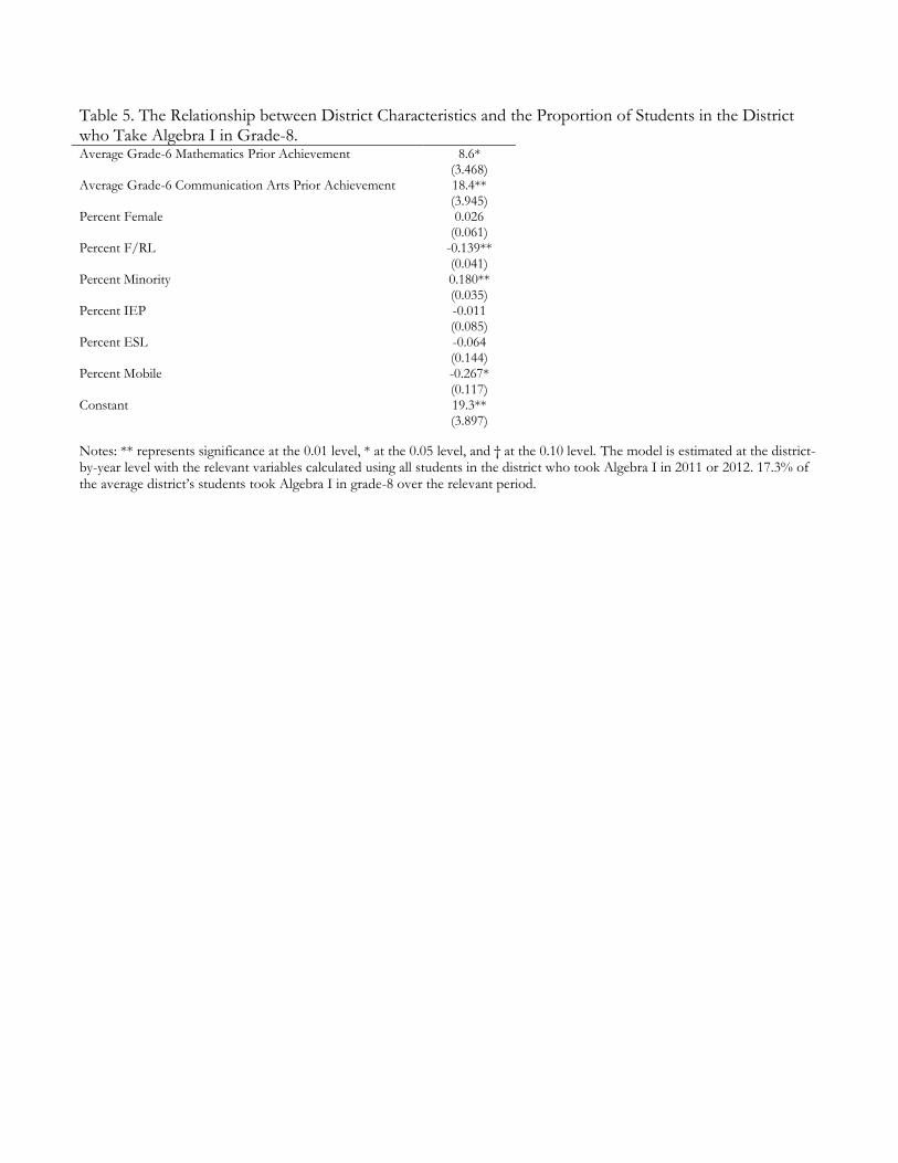
Table 5. The Relationship between District Characteristics and the Proportion of Students in the District who Take Algebra I in Grade-8.
Notes: ** represents significance at the 0.01 level, * at the 0.05 level, and † at the 0.10 level. The model is estimated at the district-by-year level with the relevant variables calculated using all students in the district who took Algebra I in 2011 or 2012. 17.3% of the average district’s students took Algebra I in grade-8 over the relevant period.
Average Grade-6 Mathematics Prior Achievement 8.6* (3.468)
Average Grade-6 Communication Arts Prior Achievement 18.4** (3.945)
Percent Female 0.026 (0.061)
Percent F/RL -0.139** (0.041)
Percent Minority 0.180** (0.035)
Percent IEP -0.011 (0.085)
Percent ESL -0.064 (0.144)
Percent Mobile -0.267* (0.117)
Constant 19.3** (3.897)

Table 6. Distribution of the Grade in which Algebra I is Taken among Initially High-Performing Students.
Grade Taken Frequency Percentage 7th or earlier 198 3.6%
8th 3516 64.2 9th 1473 26.9
10th or later 291 5.3

Table 7. Student Characteristics of Initially High-Performing Students by the Distribution of the Grade in which Algebra I is Taken.
Baseline
Sample Averages
Algebra I Taken:
Early Grade-9 Late n=5478 n=3714 n=1473 n=291 Maintained High Performance 61.2% 68.8%** 44.2% 49.5%† Percent White 92.0 91.7† 93.3 88.7* Percent Black 3.5 3.3 3.7 4.5 Percent Hispanic 1.3 1.2 1.0 3.8* Percent Asian 2.9 3.5** 1.4 2.8 Percent Female 47.8 49.1* 45.4 43.0 Percent F/RL Eligible 29.6 26.5** 35.0 42.6* Notes: ** indicates that the means are significantly different at the 0.01 level, * at the 0.05 level, and † at the 0.10 level. For the “Algebra I Taken” panel, both the “Early” and “Late” group means are compared to the means from the “Grade-9” group. To avoid confusion, significant differences in comparison to the “Grade-9” group are only marked in the “Early” and “Late” columns. In addition, the percent F/RL eligible value is based on if the student ever met that criterion over the course of the panel.
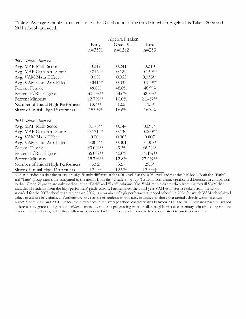
Table 8. Average School Characteristics by the Distribution of the Grade in which Algebra I is Taken. 2006 and 2011 schools attended.
Algebra I Taken: Early Grade-9 Late n=3371 n=1282 n=253 2006 School Attended Avg. MAP Math Score 0.249 0.241 0.210 Avg. MAP Com Arts Score 0.212** 0.189 0.129** Avg. VAM Math Effect 0.057 0.053 0.035** Avg. VAM Com Arts Effect 0.041** 0.033 0.019** Percent Female 49.0% 48.8% 48.9% Percent F/RL Eligible 30.3%** 34.6% 38.2%* Percent Minority 12.7%** 10.0% 21.4%** Number of Initial High Performers 13.4** 12.5 11.5* Share of Initial High Performers 15.9%* 16.6% 16.3% 2011 School Attended Avg. MAP Math Score 0.178** 0.144 0.097* Avg. MAP Com Arts Score 0.171** 0.130 0.060** Avg. VAM Math Effect 0.006 0.003 0.007 Avg. VAM Com Arts Effect 0.006** 0.001 -0.008* Percent Female 49.0%** 49.3% 48.2%* Percent F/RL Eligible 36.0%** 40.0% 45.1%** Percent Minority 15.7%** 12.8% 27.2%** Number of Initial High Performers 33.2 32.7 29.5* Share of Initial High Performers 12.9% 12.9% 12.3%† Notes: ** indicates that the means are significantly different at the 0.01 level, * at the 0.05 level, and † at the 0.10 level. Both the “Early” and “Late” group means are compared to the means from the “Grade-9” group. To avoid confusion, significant differences in comparison to the “Grade-9” group are only marked in the “Early” and “Late” columns. The VAM estimates are taken from the overall VAM that excludes all students from the high performers’ grade cohort. Furthermore, the initial year VAM estimates are taken from the school attended for the 2007 school year, rather than 2006, as a number of high performers attended schools in 2006 for which VAM school-level values could not be estimated. Furthermore, the sample of students in this table is limited to those that attend schools within the same district in both 2006 and 2011. Hence, the differences in the average school characteristics between 2006 and 2011 indicate structural school differences by grade configurations within districts, i.e. students progressing from smaller, neighborhood elementary schools to larger, more diverse middle schools, rather than differences observed when mobile students move from one district to another over time.
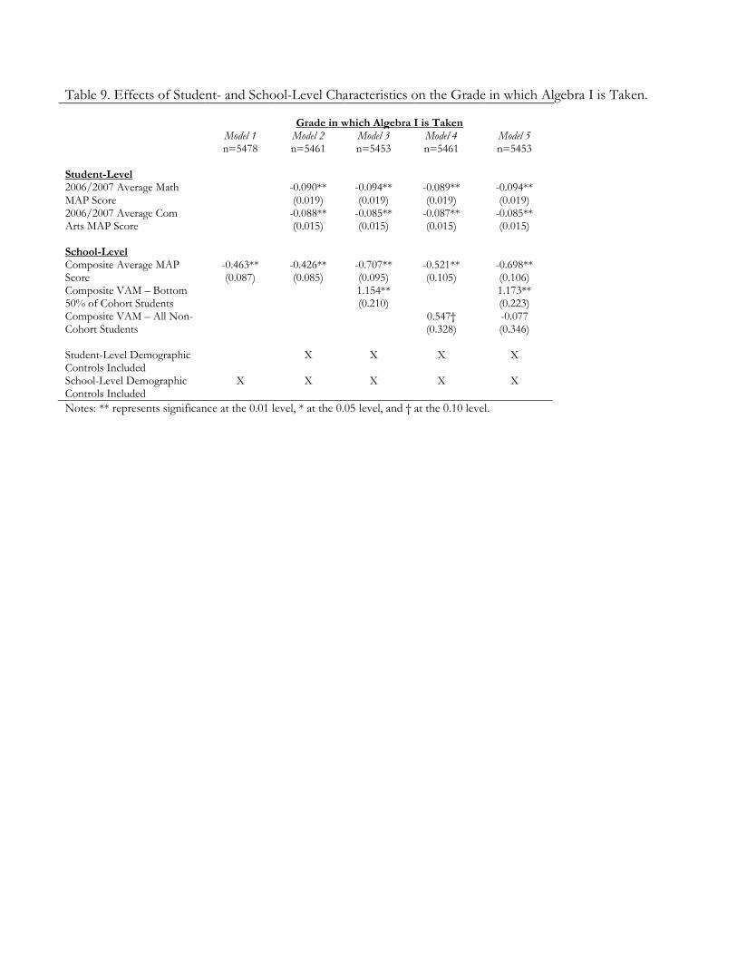
Table 9. Effects of Student- and School-Level Characteristics on the Grade in which Algebra I is Taken.
Notes: ** represents significance at the 0.01 level, * at the 0.05 level, and † at the 0.10 level.
Grade in which Algebra I is Taken Model 1 Model 2 Model 3 Model 4 Model 5 n=5478 n=5461 n=5453 n=5461 n=5453 Student-Level 2006/2007 Average Math MAP Score
-0.090** (0.019)
-0.094** (0.019)
-0.089** (0.019)
-0.094** (0.019)
2006/2007 Average Com Arts MAP Score
-0.088** (0.015)
-0.085** (0.015)
-0.087** (0.015)
-0.085** (0.015)
School-Level Composite Average MAP Score
-0.463** (0.087)
-0.426** (0.085)
-0.707** (0.095)
-0.521** (0.105)
-0.698** (0.106)
Composite VAM – Bottom 50% of Cohort Students
1.154** (0.210)
1.173** (0.223)
Composite VAM – All Non-Cohort Students
0.547† (0.328)
-0.077 (0.346)
Student-Level Demographic Controls Included
X X X X
School-Level Demographic Controls Included
X X X X X