
DOCUMENTOS DE TRABAJOsi2.bcentral.cl/public/pdf/documentos-trabajo/pdf/dtbc798.pdf · La...
33
DOCUMENTOS DE TRABAJO The Impact of Warnings Published in a Financial Stability Report on the Loan to Value Ratio Andrés Alegría Rodrigo Alfaro Felipe Córdova N.º 798 Febrero 2017 BANCO CENTRAL DE CHILE
Transcript of DOCUMENTOS DE TRABAJOsi2.bcentral.cl/public/pdf/documentos-trabajo/pdf/dtbc798.pdf · La...

DOCUMENTOS DE TRABAJO
The Impact of Warnings Published in a Financial Stability Report on the Loan to Value Ratio
Andrés AlegríaRodrigo AlfaroFelipe Córdova
N.º 798 Febrero 2017BANCO CENTRAL DE CHILE

BANCO CENTRAL DE CHILE
CENTRAL BANK OF CHILE
La serie Documentos de Trabajo es una publicación del Banco Central de Chile que divulga los trabajos de investigación económica realizados por profesionales de esta institución o encargados por ella a terceros. El objetivo de la serie es aportar al debate temas relevantes y presentar nuevos enfoques en el análisis de los mismos. La difusión de los Documentos de Trabajo sólo intenta facilitar el intercambio de ideas y dar a conocer investigaciones, con carácter preliminar, para su discusión y comentarios.
La publicación de los Documentos de Trabajo no está sujeta a la aprobación previa de los miembros del Consejo del Banco Central de Chile. Tanto el contenido de los Documentos de Trabajo como también los análisis y conclusiones que de ellos se deriven, son de exclusiva responsabilidad de su o sus autores y no reflejan necesariamente la opinión del Banco Central de Chile o de sus Consejeros.
The Working Papers series of the Central Bank of Chile disseminates economic research conducted by Central Bank staff or third parties under the sponsorship of the Bank. The purpose of the series is to contribute to the discussion of relevant issues and develop new analytical or empirical approaches in their analyses. The only aim of the Working Papers is to disseminate preliminary research for its discussion and comments.
Publication of Working Papers is not subject to previous approval by the members of the Board of the Central Bank. The views and conclusions presented in the papers are exclusively those of the author(s) and do not necessarily reflect the position of the Central Bank of Chile or of the Board members.
Documentos de Trabajo del Banco Central de ChileWorking Papers of the Central Bank of Chile
Agustinas 1180, Santiago, ChileTeléfono: (56-2) 3882475; Fax: (56-2) 3882231

Documento de Trabajo
N° 798
Working Paper
N° 798
The impact of warnings published in a financial stability report
on loan-to-value ratios
Andrés Alegría
Banco Central de Chile
Rodrigo Alfaro
Banco Central de Chile
Felipe Córdova
Banco Central de Chile
Abstract
This paper shows how central bank communications can play a role in macroprudential supervision.
We document how specific warnings about real estate markets, published in the Central Bank of
Chile’s Financial Stability Reports of 2012, affected bank lending policies. We provide empirical
evidence of a rebalancing in the characteristics of mortgage loans granted, with a reduction in the
number of mortgage loans with high loan-to-value ratios (LTV), along with an increase in loans with
lower LTV ratios.
Resumen
Este trabajo presenta evidencia sobre como los mensajes emitidos por bancos centrales pueden jugar
un rol en la supervisión macro prudencial. Documentamos el canal a través del cual ciertos mensajes
específicos, referentes al mercado inmobiliario, publicados en el Informe de Estabilidad Financiera
del Banco Central de Chile durante el 2012, afectaron las políticas de otorgamiento de crédito de los
bancos. Encontramos evidencia empírica de un rebalanceo en las características de los créditos
hipotecarios entregados, con una reducción en aquellos con alta razón préstamo a garantía, en favor
de un aumento en los de menor razón.
The views are those of the authors and do not necessarily represent those of the Central Bank of Chile. We would like to
thank Michael Ehrmann for reviewing an earlier version of this paper and providing insightful suggestions that greatly
improved this work. Comments received from several participants at the Closing Conference of the BIS CCA CGDFS
Working Group: The impact of macroprudential policies: an empirical analysis using credit registry data, are appreciated.
We also want to thank Claudio Raddatz and Jorge Bravo. The authors’ e-mail addresses are [email protected],

1
1. Introduction
Since the onset of the Great Recession, there has been a heated debate on how to prevent the
risk of instability from propagating across financial markets and how best to assure financial
stability in the future. Central banks, which have taken a central role in this discussion, have
made increasing use of communications as an additional policy tool to restore stability. In
particular, through the publication of Financial Stability Reports (FSR) and also in speeches
and interviews, policymakers have made efforts to convey their views on the potential risks
faced by the financial system.
Considering the relevance to central banks of the effective design and implementation of
macroprudential policies, the relative novelty of these tools and the breadth of the definition
of macroprudential policies, it is natural to ask how far they have been successful in conveying
their messages and achieving the intended effects.
The main aim of this paper is to measure the effect on local financial markets of
communicational tools used by the Central Bank of Chile (CBC) . In particular, this paper
focuses on the local housing market. By using a detailed administrative database of every
housing transaction in the country, we study the extent to which warnings issued in the
central bank’s Financial Stability Reports had an effect on house prices, lending standards, and
the volume of mortgage loans.
Since the onset of the subprime crisis, the real estate sector has received increasing attention
from academics and policymakers, for at least three reasons. First, the bursting of the housing
bubble in several economies initiated a process of deleveraging that led to deep
macroeconomic adjustments. Second, as housing is the main asset of the average household;
changes in property values considerably affect total household wealth. Third, a significant
amount of home purchases are financed with mortgage loans, so that banks are significantly
exposed to this sector. Since 2010, the Central Bank of Chile, through its Financial Stability
Report (FSR), has documented sustained and above-trend growth rate in house prices. Again
through the FSR, the central bank has analyzed the different constituent components of
housing prices and warned that recent developments in house price trends should not be
extrapolated for future investment decisions, i.e. that agents should not expect the recent
trends to continue unchanged in the future.

2
The paper starts by looking at the evolution of aggregate variables related to the real estate
sector around the issuance time of the warnings. Included in this analysis are housing debt
decomposed by financing instrument, the number of mortgage loans granted, average housing
debt, house prices and volume of home sales. In principle, the warnings did not seem to have
any effect on these broad variables, supporting the view that the evolution of these variables
was consistent with macroeconomic fundamentals. However, when looking more closely at
the distribution of loan-to-value (LTV) ratios of loans granted, the messages conveyed
through the FSR seem to have had an impact. Using a detailed administrative database for
mortgage loan transactions, this paper shows that FSR warnings had an effect on bank lending
policies between 2011 and 2014. In particular, following the FSR warnings, there was a
noticeable reduction in the number of loans granted with high LTV ratios. Later, the analysis
is formalized using probit and quantile regressions; these estimations confirm the previous
findings. The warnings had a statistically significant effect, reshaping the distribution of LTV
ratios for loans granted. In particular, during the period there is evidence of a shift out of
mortgages with high LTVs, and into lower ratios. Furthermore, private banks and the state-
owned bank responded differently to these messages, most likely due to the mandate under
which the latter institution operates.
2. Chilean Real Estate Market
2.1 Housing finance
Since the early 1990s, the Chilean housing market has experienced significant developments
in several aspects. In particular, Micco et al (2012) show that: (i) the fraction of overcrowded
houses1 dropped from 24% to 9% between 1990 and 2009, and (ii) the housing deficit2
decreased from 540 thousand units to 410 thousand units. In addition, the Survey of Housing
Finance conducted by the Central Bank of Chile indicates in its 2014 wave that
homeownership rate was about 70%. According to Warnock (2014) this figure is at the top
among Latin-American countries. A key element of this homeownership rate is the access to
1 According to the National Socioeconomic Characterization (CASEN) Survey, conducted in Chile and used by Micco et al. Overcrowded houses are defined as those where the ratio of residents over the number of bedrooms in a house exceeds 2.5.
2 Micco et al. define housing deficit as the difference between total population and the stock of habitable permanent houses (excluding mobile units and those located in slums).

3
housing finance. Several elements must be considered in order to understand the Chilean
mortgage market. First, there is a unit of account indexed to inflation (UF3) in which banks
and financial institutions can grant long-term (20-30 years) loans. Second, most of this market
is dominated by banks, having a share of 88% of mortgage loans as of 2010 and a historical
average of 90% since early 2000 (Graph 1). Given these facts, the following description will be
focused on the banking sector. Among banks, a big player is BancoEstado (BE), a state-owned
bank with a participation of 24% over total banking mortgage loans (Table 1).
Table 1: Total and mortgage loans by bank, as of December 2010
TOTAL LOANS MORTGAGE LOANS
BANK US$ Millions Percent US$ Millions Percent
Banco Bice 4,516 2.7% 473 1.2%
BBVA 12,277 7.4% 3,342 8.1%
Consorcio 257 0.2% 52 0.1%
De Chile 32,888 19.8% 6,144 15.0%
BCI 20,377 12.2% 4,030 9.8%
BancoEstado 23,647 14.2% 9,762 23.8%
Falabella 1,421 0.9% 482 1.2%
Internacional 1,381 0.8% 7 0.0%
Itaú (Chile) 5,895 3.5% 1,181 2.9%
Paris 383 0.2% 28 0.1%
Ripley 419 0.3% 119 0.3%
Santander - Chile 35,739 21.5% 9,796 23.9%
Security 4,621 2.8% 633 1.5%
Corpbanca 12,504 7.5% 2,144 5.2%
HSBC Bank (Chile) 686 0.4% 2 0.0%
Scotiabank Chile 8,195 4.9% 2,837 6.9%
Others 1,149 0.7% 1 0.0%
Total 166,355 100% 41,032 100%
Source: Central Bank of Chile.
Third, a number of mortgage-instruments are available for financing the purchase of a house:
mortgage notes, endorsable mortgage loans, and non-endorsable mortgage loans. Mortgage
notes can be used to finance a fraction of the value of the property, having a maximum
allowed Loan to Value of 75%; there is also a limit on Dividend to Income (DTI) of 25% for
small and medium size loans. Endorsable mortgage loans have a maximum LTV of 80% and no
3 Unidad de Fomento (UF) is a unit of account used in Chile. Its value in Chilean pesos is indexed to total inflation. It is widely used in determining the value of real estate, housing associated costs, and secured loans.

4
limit on DTI. Finally, non-endorsable mortgage loans have no limit on LTV nor on DTI. During
the early 2000s, most housing funding was granted through mortgage notes, but since 2004
there has been an increasing participation of non-endorsable mortgage loans. One reason
behind this composition change is the combination of an increased credit demand and the
relatively larger flexibility of non-endorsable mortgage loans, in terms of LTV and DTI limits,
length of term, interest rates, and minimum down payment requirement. The shift also
coincides with the introduction, in November 2002, of a transaction tax exemption to loan
renegotiations. According to Flores (2006) who studies the evolution of the housing market
financing instruments in more detail, both new and existing mortgage loans financed through
mortgage notes rapidly switched to non-endorsable mortgage loans after the implementation
of the tax exemption mentioned above (Graph 1).
In addition to the stock figures presented in Table 1, information on flows between 2011 and
2014 (period under study) shows that eight banks accounted for about 95% of the total
transactions and 93% of the total amount lent (Graph 2). This distribution allows us to focus
on this subset of banks for our methodological framework, including the state-owned bank
(BancoEstado, BE). It should be noted that the participation of BE in the total number of loans
is about 33%, but weighted by amount is only 17%. That implies that BE tends to grant loans
of relatively small size.

5
Graph 1: Banking housing debt by
instrument
(percent)
Graph 2: Number of loans by bank in
sample4
(cumulative percent)
Source: Superintendency of Banks.
Source: Chilean Tax Authority.
Focusing on the period between years 2011 and 2014, mortgage debt showed steady growth,
reaching real annual variations close to 9%. This growth is mainly due to the increase in
average debt, as opposed to number of debtors (Graph 3). Although this is consistent with the
evolution of housing prices discussed below, there was an increment in the number of
mortgage loans by debtor. Indeed, the fraction of debtors with more than one mortgage has
increased from 19 to 23% (Graph 4).
4 Unweighted is the cumulative percentage of number of loans granted by each bank. Weighted is the cumulative percentage of the number of loans granted, weighted by the total sum of loan flows corresponding to each bank.
0
25
50
75
100
01 03 05 07 09 11 13 15
Non endorsable mortgage loans Mortgage notes
Endorsable mortgage loans
0
25
50
75
100
BE B1 B3 B4 B5 B6 B7 B8 B9 B10 B11 B12 B13 B14 B15
Unweighted
Weighted

6
Graph 3: Mortgage loans
(real annual variation, percent)
Graph 4: Mortgage loans by debtor
(percent)
Source: Central Bank of Chile. Source: Superintendency of Banks.
2.2 Housing Price Index
The Chilean Tax Authority maintains a detailed administrative database of every housing
transaction in the country. The database includes information related to the transaction, such
as price, location of the house, etc. It also includes information about the characteristics of the
house, such as: size (measured in squared meters), or type (apartment, town house). Finally,
in this database there is information related to the conditions of the loan (if applies), such as:
maturity and bank name. With this information it is straightforward to compute the LTV ratio
per transaction.
Using the Chilean Tax database, the Central Bank of Chile calculates the housing price index
(HPI) using a methodology known as stratified method or mix-adjustment5. This methodology
measures the variations of prices of different types of houses by splitting the sample in groups
by certain characteristics, such as, price, geographical location, size, etc. This methodology,
therefore, controls for changes in the composition of the sold houses between periods not in
groups. For each group average price is computed and we obtain an aggregate index by
weighting averages across groups. Further, the sample is divided into seven geographic zones:
North, Center, South and the Metropolitan Area (M.A.)6 which is divided in M.A. East, M.A
5 For more details about methodology see Central Bank of Chile (2013).
6 The Metropolitan Area is the most densely populated in Chile.
0
2
4
6
8
10
12
11 12 13 14 15
Debtors Average debt
Total variation Warnings
60
70
80
90
100
11 12 13 14 15
1 2 >2

7
West, M.A Downtown and M.A South7. Also, each zone is divided between town-houses and
apartments, getting a grand total of 14 groups. This allows the CBC to construct the HPI by
zone and type of house, the aggregation is performed weighting these by squared meters. In
addition to this index, there is a private estimate of house prices generated by the Chilean
Chamber of Construction (CChC). The latter is computed only for M.A. and it is based on new
houses only. In addition, the index includes houses that are still under construction
(promises), we use this additional source since the latter information is not available in our
Chilean Tax database.
According to the different sources mentioned above, aggregate prices have shown growth
rates consistent with increasing national private income and low long-term interest rates
(Graphs 5 and 6)8. The previous factors, combined with changes in the sales tax policy had an
impact on the sale of housing units in Santiago, which have shown a positive trend since 2009
(Graph 7). However, the national figures hide substantial heterogeneity across zones, which is
probably influenced by differences in the behavior of demand and the relative supply in each
of them. Del Negro and Otrok (2007) documented this heterogeneity in the U.S. Their findings
indicate that the factors driving house prices switch over time from local to national sources;
the national variation does not seem to be linked to monetary policy changes. Allen et al.
(2009) also explore this regional price heterogeneity using Canadian data, they find little
evidence of long run correlation between different cities and also document a disconnect
between house prices, interest rates and other macroeconomic variables. Local factors such as
union wage levels, new housing prices and number of building permits issued seem to be
more closely related to local house prices. Regarding our dataset, despite differences in
methodologies of both indexes, they show similar trends. However, the one computed by
CChC shows fewer fluctuations, most likely because it is based on a fitted model.
7 More details about the subdivision into zones see Central Bank of Chile (2013). A detailed map depicting the different zones is included for reference in Appendix 1.
8 For further details see Chapter III in Financial Stability Report (2013:S2).

8
Graph 5: Comparison of HPIs9 (*)
(index; 100 = 2008)
Graph 6: House price index by zone (*)
(index; 100 = 2008)
Sources: Central Bank of Chile and CChC. Source: Central Bank of Chile.
(*) Central Bank of Chile information as of June 8, 2016.
Between 2011 and 2014, new home sales and construction in Santiago remained close to
60,000 per year. The production of new homes, including gross commitments, grew strongly
during the period. . Finally, relative to disposable income, housing prices were stable within
our sample and in the lower range of indicators for a wide set of countries.10
9 CChC uses a hedonic methodology to calculate the index, as opposed to the other indices where a stratified methodology is utilized.
10 For further details see Chapter III in Financial Stability Report (2015:S1).
40
60
80
100
120
140
160
180
02 03 04 05 06 07 08 09 10 11 12 13 14 15 III
Warnings CChC
HPI Metropolitan area
40
60
80
100
120
140
160
180
02 03 04 05 06 07 08 09 10 11 12 13 14 15 III
Warnings North zoneCenter zone South zoneMetropolitan area

9
Graph 7: Sales by type of property
(units)
(*) Include promises. Source: Chilean Chamber of Construction.
2.3 Warnings in the Financial Stability Report
Twice a year, the CBC publishes its Financial Stability Report (FSR). The objective of the FSR is
to provide information to the general public, on a half-yearly basis, on recent macroeconomic
and financial events that could affect the financial stability of the Chilean economy. In
addition, the FSR presents policies and measures that support the normal operation of the
internal and external payment system. In the first and second half of 2012 two warnings were
published in the FSR, they were associated with the real estate market and its developments
(Table 2). Both referred to the existence of potential risks in the housing market, and the
second one explicitly mentioned lending standards. The warnings were also included in the
Reports’ summaries, not just within the corresponding chapters. Regarding the resonance of
the warnings in the media, they were widely covered in newspapers, television news and
specialized magazines. These messages were also delivered by the Members of the Board in
their presentations and speeches in the days following the issuance of the Reports. It is hard
to quantify the intensity of the messages just by reading the warnings. That is why we will
take a quantitative approach in order to do this.
0
5,000
10,000
15,000
20,000
25,000
09 10 11 12 13 14 15
Apartments Houses

10
Table 2: FSR Warnings
First Half 2012 (June 18, 2012)
Second Half 2012 (December 18, 2012)
“Aggregate housing prices move in tandem with the economy’s level of interest rates and income. At some districts in the central and eastern area of the Santiago Metropolitan Region prices are outgrowing their historic trends, possibly due to constraints in the land available. It is important to keep in mind that the materialization of the risk scenario described in this Report could lead to a breakdown in current price trends. The potential implications of this are price adjustments influencing the profits of executed projects and, additionally, the collaterals backing mortgage loans”.
“The Report highlights that aggregate housing prices indices have maintained their pace of expansion, in line with the dynamism of the economy, and that in many districts prices are rising above historic trends. These increases occur in a context of high growth in housing demand and a significant expansion of activity in this sector. […] This, together with somewhat less stringent lending standards for mortgage credit. These developments could lead to financial vulnerabilities in the real estate and construction industry, or in those households searching for a home”.
Source: Central Bank of Chile.
As we showed in the previous section, these warnings do not seem to have had an effect on
aggregate house prices or the total volume of mortgage loans granted. The warning issued in
June 2012 is marked in Graph 5 with a red bar; there is no noticeable effect on aggregate
housing prices. The same lack of variation is observed when house prices are decomposed by
zone (Graph 6). The second warning —also marked with a red bar— does not appear to have
an impact on prices either. Graph 3 shows the growth rate of mortgages loans accelerating
following the issuance of warnings. Thus, the aggregate figures suggest that warnings had no
impact, and Central Bank communication through the FSR was ineffective as a
macroprudential tool. There are two possible explanations for this. First, the warnings may
not have had enough power because market participants did not value the messages delivered
in the FSR. This would imply a failure of warnings as a feasible macroprudential tool. Second,
these warnings may have had no impact on these aggregate variables because the warnings
did not point to an existing imbalance in the market, but to the risks of such an imbalance.
Thus, it is expected that warnings of this sort would affect the lending policies of banks, for
instance on Loan to Value ratio.

11
By considering the information of the eight largest banks in this market, the distribution of
LTV ratios for newly originated mortgages showed some variation around the two warning
events. In particular, the high-end of the LTV distribution (90th percentile) fell after the first
warning and then dropped again after the second warning (Graph 8). It is worth noting that
the 75th percentile did not react to these warnings, being a compression of high LTV‘s. Prior
to the first warning, about 10% of mortgage loans were granted with an LTV of 100%, after
the warnings around 10% of loans were granted with an LTV of 90%. Concerned about a
possible bias in our results due to the presence of the state owned bank (BE), which in
previous crisis episodes has shown a different behavior compared to the rest of the banking
system11, we removed it from the sample. When re-estimating with this trimmed sample, the
impact remains (Graph 9).
Graph 8: LTV full sample (*)
(percent)
Graph 9: LTV without BE (*)
(percent)
(*) Vertical lines indicate the warnings dates.
Source: Central Bank of Chile.
11 Also in the past, it was documented that BE had a higher NPL ratio in its portfolio of housing loans compared to other banks. Moreover, in the same post crisis period, credit growth would have been weaker without BE. These facts are evidence of a different behavior of BE in terms of lending conditions (see Financial Stability Report First Half 2010).
40
50
60
70
80
90
100
11 III 12 III 13 III 14
P10, P90 P75 Median
40
50
60
70
80
90
100
11 III 12 III 13 III 14
P10, P90 P75 Median
12
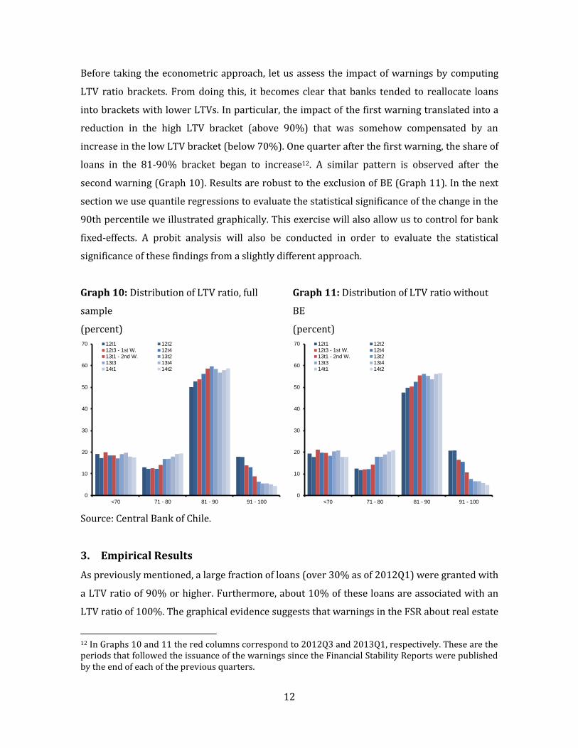
Before taking the econometric approach, let us assess the impact of warnings by computing
LTV ratio brackets. From doing this, it becomes clear that banks tended to reallocate loans
into brackets with lower LTVs. In particular, the impact of the first warning translated into a
reduction in the high LTV bracket (above 90%) that was somehow compensated by an
increase in the low LTV bracket (below 70%). One quarter after the first warning, the share of
loans in the 81-90% bracket began to increase12. A similar pattern is observed after the
second warning (Graph 10). Results are robust to the exclusion of BE (Graph 11). In the next
section we use quantile regressions to evaluate the statistical significance of the change in the
90th percentile we illustrated graphically. This exercise will also allow us to control for bank
fixed-effects. A probit analysis will also be conducted in order to evaluate the statistical
significance of these findings from a slightly different approach.
Graph 10: Distribution of LTV ratio, full
sample
(percent)
Graph 11: Distribution of LTV ratio without
BE
(percent)
Source: Central Bank of Chile.
3. Empirical Results
As previously mentioned, a large fraction of loans (over 30% as of 2012Q1) were granted with
a LTV ratio of 90% or higher. Furthermore, about 10% of these loans are associated with an
LTV ratio of 100%. The graphical evidence suggests that warnings in the FSR about real estate
12 In Graphs 10 and 11 the red columns correspond to 2012Q3 and 2013Q1, respectively. These are the periods that followed the issuance of the warnings since the Financial Stability Reports were published by the end of each of the previous quarters.
0
10
20
30
40
50
60
70
<70 71 - 80 81 - 90 91 - 100
12t1 12t212t3 - 1st W. 12t413t1 - 2nd W. 13t213t3 13t414t1 14t2
0
10
20
30
40
50
60
70
<70 71 - 80 81 - 90 91 - 100
12t1 12t212t3 - 1st W. 12t413t1 - 2nd W. 13t213t3 13t414t1 14t2

13
market vulnerabilities made by the Central Bank of Chile had an impact on the high end of the
LTV distribution. To document whether these warnings had a significant impact, two different
methodologies are used in this section. First, a binary probit model is estimated in order to
quantify the effectivity of public warnings about potential housing market vulnerabilities had
in diminishing the probability that a high LTV ratio loan was granted. In this model a positive
outcome is defined as the granting of a loan with an LTV ratio exceeding a given threshold.
Second, as we showed in the previous section, the central moments of the LTV ratio
distribution remained unchanged with the effects concentrated on its upper tail. Thus, a
quantile regression is estimated in order to compute the impact of the public warnings on the
median and several other percentiles of the LTV ratio distribution. Attending to the historical
behavior of the state owned bank, a robustness exercise excluding BancoEstado is conducted
for both probit and quantile estimations. In the estimations below we use the Chilean Tax
Authority data. Regarding our implicit counterfactual scenario, following others in the related
literature, such as Best et al. (2015), Wong et al. (2015) and Price (2014), we define an
implicit counterfactual of no change in the LTV distribution after the issuance of the warnings.
This is underlying the definition of our dummy variables. The pre-warning level can be
computed as the case where the corresponding dummy variable is equal to zero. The sample
includes all mortgage loan transactions that took place between 2011 and 2014 with daily
frequency.
3.1 Binary Modeling for Loan to Value Ratio
In this section we estimate a probit model. We do not use OLS since the LTV variable is
bounded above at 100 by the Chilean regulation. Our dependent variable is binary, it is equal
to 1 when the LTV ratio associated to a transaction is higher than a given threshold, and 0
otherwise. We construct two dependent variables for two LTV thresholds, namely LTV90 and
LTV80 for 90 and 80% thresholds, respectively. All of the results corresponding to probit
models are estimated coefficients, they are not marginal effects.
As independent variables, we construct two dummy variables, one for each FSR warning. The
first one was issued in 2012Q2, and the second in 2012Q4. Each of the corresponding dummy
variables is equal to 1 after the respective warning is issued and 0 otherwise13. In tables 3 and
13 In the result tables shown below the dummy variables are labeled 2012Q3 and 2013Q1, respectively, to reflect the fact that they are equal to one starting on the quarter that follows the issuance of each warning.

14
4 results are presented for the sample containing all 8 banks, as well as the sample excluding
BE. For the LTV90 estimation, in column 1 we can see the first warning reduced the
probability of a loan being granted with an LTV higher than 90%. In columns 2 and 3 we
report how the second warning also had a significant negative effect on the probability of
occurrence. The sign for the first warning switches to positive; however the joint effect of both
warnings remains negative and statistically significant. Furthermore, the estimation excluding
BE shows a robust result, with a larger magnitude for the total effect than the one obtained
with the full sample. The fact this effect is larger without the state owned bank could be due to
its mandate, and segment of the mortgage loan market where it operates. Next we show the
estimation results for the 80% threshold in Table 4. For the model in column 1, with the first
warning only, the effect is positive. This result is puzzling, but could be explained by a
reallocation of loans, with banks granting more loans with lower LTV to compensate for the
reduction in those with a higher ratio. This result follows the same pattern when we include
both warnings in columns 2 and 3; there is a positive sign for the first warning and negative
for the second, both statistically significant. When we estimate excluding BE, the impact of
each warning over the probability of occurrence is individually negative and significant. Once
again this could be due to the mandate that rules the state owned bank BE.
Table 3: Probit - (LTV90)
Full Sample Without BE (1) (2) (3) (4) (5) (6) 2012q3 -0.07*** 0.04*** 0.06*** -0.22*** -0.06*** -0.04*** (0.01) (0.01) (0.01) (0.01) (0.01) (0.01) 2013q1 -0.16*** -0.16*** -0.21*** -0.22*** (0.01) (0.01) (0.01) (0.01) Constant -0.25*** -0.25*** -0.04*** -0.19*** -0.19*** 0.02*** (0.00) (0.00) (0.01) (0.00) (0.00) (0.01) Bank FE - - Yes - - Yes N 198,299 198,299 198,299 157,985 157,985 157,985
Note: Table shows in Columns (2) and (3) how the second warning had a significant and negative effect on the right tail of the LTV distribution. Columns (5) and (6) show how this effect is larger when we exclude the state-owned bank. *, **, *** indicate statistical significance at 10, 5, and 1% levels, respectively. Standard error in parenthesis. Source: Author’s calculations.

15
Table 4: Probit – (LTV80)
Full Sample Without BE (1) (2) (3) (4) (5) (6) 2012q3 0.05*** 0.09*** 0.11*** -0.12*** -0.08*** -0.06*** (0.01) (0.01) (0.01) (0.01) (0.01) (0.01) 2013q1 -0.05*** -0.06*** -0.05*** -0.07*** (0.01) (0.01) (0.01) (0.01) Constant 0.50*** 0.50*** 0.62*** 0.62*** 0.62*** 0.69*** (0.00) (0.00) (0.01) (0.00) (0.00) (0.01) Banks FE - - Yes - - Yes N 198,299 198,299 198,299 157,985 157,985 157,985
Note: Table shows in Columns (2) and (3) how the second warning had a significant and negative effect on the right tail of the LTV distribution. Columns (5) and (6) show how this effect is also negative and significant for the first warning. *, **, *** indicate statistical significance at 10, 5, and 1% levels, respectively. Standard error in parenthesis. Source: Author’s calculations.
3.2 Quantile regression
The main objective of the analysis in this sub-section is to study how the FSR warnings
affected the distribution of LTV ratios for newly originated mortgage loans, focusing on the
upper tail of this distribution. In particular, we consider quantile regression analysis for the
90, 75 and 50th percentiles14. We show additional results for the 85 and 80th percentiles in
Appendix 2.
As dependent variable we use the LTV ratio of granted mortgage loans. Independent variables
are the same we used when estimating the probit model, dummy variables for each of the two
warnings issued by the Central Bank of Chile. As we showed in Graphs 9 and 10, the median
and 75th percentile LTV ratios remain almost constant after both warnings. This is a desirable
outcome since the warnings did not aim towards correcting a misalignment in the less risky
brackets of LTV. Instead, the second warning explicitly mentioned the somewhat less
stringent lending standards for mortgage credit, which in turn is associated with the upper
tail of the LTV ratio distribution.
Our results in Table 5 suggest that the FSR warnings were relevant reducing the LTV of loans
granted with ratios above 90% (graphically shown above in Graph 8). Column 2 shows how
both warnings significantly reduced the 90th percentile of the LTV ratio distribution, for this
14 We consider the quantile regression framework, as opposed to linear regression, because our focus is on upper-tail events. The quantile regression estimation algorithm we utilize is the one available by default in Stata 14.

16
specification we cannot reject that the effects of both warnings are equal to each other. The
effect of the second warning becomes relatively larger in Column 3, with respect to the first,
when we add bank level fixed effects, in fact now we reject the null of equal effects. Similar to
the probit specification, the effect of the second warning becomes larger, relative to the first
one, when we exclude BE from the sample (columns 4 through 6)15, which historically has
had a behavior different from that of private banks. As mentioned above, this different effect
could be due to the explicit mention to less stringent lending standards included in the second
warning. This element, combined with the different nature of the state owned bank, are
plausible explanations to why the effects are larger when BE is excluded.
Table 5: Quantile Regression - (Q90)
Full Sample Without BE (1) (2) (3) (4) (5) (6) 2012q3 -9.87*** -4.95*** -0.63*** -9.48*** -3.89*** -1.07*** (0.05) (0.08) (0.14) (0.03) (0.05) (0.18) 2013q1 -4.95*** -1.36*** -6.06*** -5.00*** (0.09) (0.15) (0.05) (0.19) Constant 99.95*** 99.95*** 100.00*** 100.00*** 100.00*** 100.00*** (0.04) (0.03) (0.11) (0.02) (0.02) (0.12) Banks FE - - Yes - - Yes N 198,299 198,299 198,299 157,985 157,985 157,985
Note: Table shows in Columns (2) and (3) how the second warning had a significant and negative effect on the right tail of the LTV distribution. Columns (5) and (6) show how this effect is relatively larger for the second warning, compared with the first, when we exclude the state-owned bank. *, **, *** indicate statistical significance at 10, 5, and 1% levels, respectively. Standard error in parenthesis. Source: Author’s calculations.
15 In both Columns 5 and 6 we reject the null of equal effects stemming from the first and second warnings.

17
Table 6: Quantile Regression - (Q75)
Full Sample Without BE (1) (2) (3) (4) (5) (6) 2012q3 -0.02*** -0.01*** -0.00 -0.04*** -0.02*** -0.01 (0.00) (0.00) (0.04) (0.00) (0.00) (0.06) 2013q1 -0.02*** -0.01 -0.02*** -0.02 (0.00) (0.04) (0.00) (0.06) Constant 90.02*** 90.02*** 90.97*** 90.04*** 90.04*** 90.97*** (0.00) (0.00) (0.03) (0.00) (0.00) (0.04) Banks FE - - Yes - - Yes N 198,299 198,299 198,299 157,985 157,985 157,985
Note: Table shows how the negative effect of the warnings approaches zero as we move closer to the center of the LTV distribution. *, **, *** indicate statistical significance at 10, 5, and 1% levels, respectively. Standard error in parenthesis. Source: Author’s calculations.
Table 7: Quantile Regression - (Q50)
Full Sample Without BE (1) (2) (3) (4) (5) (6) 2012q3 -0.27*** 0.38*** 0.02 -1.27*** -0.14 -0.01 (0.05) (0.08) (0.12) (0.04) (0.09) (0.13) 2013q1 -1.00*** -0.13 -1.80*** -1.15*** (0.08) (0.13) (0.09) (0.14) Constant 89.54*** 89.54*** 89.99*** 89.95*** 89.95*** 90.00*** (0.03) (0.03) (0.09) (0.03) (0.04) (0.09) Banks FE - - Yes - - Yes N 198,299 198,299 198,299 157,985 157,985 157,985
Note: Table shows how the negative effect of the warnings approaches zero as we move closer to the center of the LTV distribution. *, **, *** indicate statistical significance at 10, 5, and 1% levels, respectively. Standard error in parenthesis. Source: Author’s calculations.
Then, we estimate the model for the 75th percentile, looking for movements distinct to those
in the 90th percentile in an a priori less risky bracket. As shown in Table 6, the magnitude of
the effects is smaller than those previously obtained for the 90th percentile. When we add
bank level fixed effects in column 3, the warning coefficients are no longer statistically
significant. Also, we no longer observe an important difference in estimated coefficients after
removing BE (columns 4 through 6).
Finally, results for the 50th percentile in Table 7 suggest that the first warning had a positive
and statistically significant effect over the granting of mortgage loans, but still negative when
aggregating the impact of both warnings (column 2). When we add bank fixed effects, the
effects of both warnings are no longer significant (column 3). Once again this could be due to

18
the warnings being aimed towards a riskier segment of credit. After excluding BE from the
sample (columns 4 through 6), the effect of the first warning is not statistically significant. The
second warning still has a negative and significant coefficient.
Besides the exercises presented above, we perform three additional variations. First, we re-
define the warning issuance dummy variable to be equal to one since the day the FSR is
presented to the Congress and released to the market and analysts (referred to as ‘week – for
each warning´ in Appendix 3). This variation is implemented in order to isolate other
contemporaneous developments that could also affect the LTV distribution. Secondly, also
aimed towards refining the identification of the effect, we re-estimate the models using a
tighter window of periods around the issuance of the warnings, just one quarter after and
before the warnings to be more precise (referred to as ‘tighter window’ in Appendix 3).
Finally, for completeness we estimate the quantile regression including the two refinements
just described together (namely with the dummy variable re-definition and a tighter window
around the FSR presentation date, referred to as ‘week and tighter window’ in Appendix 3).
The results are roughly the same as in the original estimations, confirming that the warnings
had a statistically significant impact on the 90th percentile of the LTV distribution, with the
second warning having a larger impact than the first one when BE is excluded. Among all the
additional exercises considered, the most relevant difference is detected when we estimate
using a tighter window and include bank fixed effects. Particularly, in this case none of the
warnings have a significant effect over the LTV distribution. In general, the results obtained
with the two variations combined are similar to those obtained using a tighter window.
19
Final remarks
The structure and behavior of the mortgage market are crucial elements to consider when
analyzing the home purchasing decision. In 2012, given the developments in the housing
market, the Central Bank of Chile through its Financial Stability Report raised concerns
regarding potential vulnerabilities in certain geographical areas. On an aggregate level, in the
real estate market as a whole, these warnings do not seem to have had an effect on the volume
of home sales or loans granted. However, at the micro level, empirical evidence suggests that
the number of loans granted with high LTV ratios was significantly reduced after the relevant
warnings were published in these reports. The mechanism underlying the latter result is one
of coordination among banks, where initially they did not internalize the potential social cost
of granting high-LTV loans. The warnings served as a way of alleviating this market failure
through communication. After the warnings were published, by the end of 2013 discussions
on the adjustment of the loan loss provision policy started.16 By the end of 2015, the proposed
modifications were made public by the Superintendency of Banks and Financial Institutions.
Among other changes, provisions were to be calculated separately for residential loans, by
using a standardized method for all banks that explicitly takes into account the share of non-
performing loans and their LTV ratios.17 The new regulation went into effect in January 2016.
Based on different methodologies, we conclude that the issued warnings had a significant
effect on bank lending policies. This finding is in line with the central bank’s decision to point
out the existence of potential risks arising from less stringent lending standards in the
extremes of the distribution.
16 Superintendencia de Bancos e Instituciones Financieras, Chile. Compendio de Normas Contables, Capítulo B-1 / 18.12.2013.
17 Superintendencia de Bancos e Instituciones Financieras, Chile. Circular N° 3.598 / 24.12.2015.

20
References
Allen, J., R. Amano, D.P. Byrne, and A.W. Gregory, 2009. "Canadian city housing prices and
urban market segmentation" Canadian Journal of Economics/Revue canadienne d'économique
42.3: 1132-1149.
Best, C., J. Cloyne, E. Ilzetzki, and H.J. Kleven, 2015. “Interest rates, debt and intertemporal
allocation: evidence from notched mortgage contracts in the United Kingdom” Bank of
England Staff Working Paper Series 543, August.
Central Bank of Chile, 2014. “Índice de Precios de Vivienda en Chile: Metodología y
Resultados”. Studies in Economic Statistics 107, June.
Central Bank of Chile. Financial Stability Report. Various issues.
Del Negro, M., C. Otrok, 2007. “99 Luftballons: Monetary policy and the house price boom
across states”, Journal of Monetary Economics, 54, 1962-1985.
Flores, C., 2006. “Financiamiento Hipotecario para la Vivienda, Evolución Reciente 1995-
2005”. Technical Studies Series N°004, Superintendency of Banks and Financial Institutions,
March.
Micco, A., E. Parrado, B. Piedrabuena, A. Rebucci, 2012. "Housing Finance in Chile:
Instruments, Actors, and Policies" Research Department Publications 4779, Inter-American
Development Bank, Research Department.
Price, G., 2014. “How has the LVR restriction affected the housing market: a counterfactual
analysis” Reserve Bank of New Zealand Analytical Note series AN2014/03, May 2014.
Superintendencia de Bancos e Instituciones Financieras, 2013. “Compendio de Normas
Contables” SBIF Chapter B-1, December 2013.
Superintendencia de Bancos e Instituciones Financieras, 2013. “Circular N° 3.598” SBIF,
December 2015.
21
Warnock F., 2014. “Housing Finance in Latin America”. IIMB-IMF Conference on Housing
Markets, Financial Stability and Growth, December.
Wong E., A. Tsang, and S. Kong, 2014. “How Does Loan-To-Value Policy Strengthen Banks'
Resilience to Property Price Shocks - Evidence from Hong Kong" Working Papers 032014,
Hong Kong Institute for Monetary Research.

22
Appendix 1
Chilean geographic zones
Source: Author´s elaboration.
Chilean geographic zones
North South
Center M.A
M.A South M.A East
M.A West M.A Downtown
Source: Author´s elaboration.

23
Appendix 2
Table A1: Quantile Regression - (Q85)
Full Sample Without BE (1) (2) (3) (4) (5) (6) 2012q3 -2.94*** -2.76*** -0.04 -5.07*** -3.16*** -2.23*** (0.14) (0.24) (0.05) (0.10) (0.20) (0.12) 2013q1 -0.18 -0.04 -1.92*** -0.42*** (0.25) (0.05) (0.21) (0.13) Constant 92.97*** 92.97*** 100.00*** 95.10*** 95.10*** 100.00*** (0.10) (0.10) (0.03) (0.07) (0.08) (0.08) Banks FE - - Yes - - Yes N 198,299 198,299 198,299 157,985 157,985 157,985
*, **, *** indicate statistical significance at 10, 5, and 1% levels, respectively. Standard error in parenthesis. Source: Author’s calculations.
Table A2: Quantile Regression - (Q80)
Full Sample Without BE (1) (2) (3) (4) (5) (6) 2012q3 -0.05*** -0.02*** -0.01 -0.83*** -0.79*** -0.10 (0.00) (0.00) (0.05) (0.06) (0.10) (0.09) 2013q1 -0.03*** -0.02 -0.04 -0.03 (0.00) (0.05) (0.11) (0.09) Constant 90.06*** 90.06*** 95.09*** 90.84*** 90.84*** 95.16*** (0.00) (0.00) (0.04) (0.04) (0.04) (0.06) Banks FE - - Yes - - Yes N 198,299 198,299 198,299 157,985 157,985 157,985
*, **, *** indicate statistical significance at 10, 5, and 1% levels, respectively. Standard error in parenthesis. Source: Author’s calculations.

24
Appendix 3
Week – for each warning
Table A3: Quantile Regression - (Q90)
Full Sample Without BE (1) (2) (3) (4) (5) (6) 2012-18-06 -9.90*** -4.97*** -0.03 -9.15*** -2.33*** 0.00 (0.05) (0.08) (0.13) (0.06) (0.06) (0.18) 2012-18-12 -4.97*** -1.92*** -7.60*** -5.71*** (0.08) (0.14) (0.06) (0.19) Constant 100.00*** 100.00*** 100.00*** 100.00*** 100.00*** 100.00*** (0.04) (0.03) (0.10) (0.04) (0.02) (0.12)
Banks FE - - Yes - - Yes N 198,299 198,299 198,299 157,985 157,985 157,985
*, **, *** indicate statistical significance at 10, 5, and 1% levels, respectively. Standard error in parenthesis. Source: Author’s calculations.
Table A4: Quantile Regression - (Q85)
Full Sample Without BE (1) (2) (3) (4) (5) (6) 2012-18-06 -2.96*** -2.46*** -0.04 -5.10*** -2.07*** -1.51*** (0.14) (0.24) (0.05) (0.10) (0.21) (0.12) 2012-18-12 -0.51** -0.04 -3.04*** -1.03*** (0.24) (0.05) (0.22) (0.13) Constant 92.99*** 92.99*** 100.00*** 95.13*** 95.13*** 100.00*** (0.10) (0.10) (0.04) (0.07) (0.09) (0.08)
Banks FE - - Yes - - Yes N 198,299 198,299 198,299 157,985 157,985 157,985
*, **, *** indicate statistical significance at 10, 5, and 1% levels, respectively. Standard error in parenthesis. Source: Author’s calculations.

25
Table A5: Quantile Regression - (Q80)
Full Sample Without BE (1) (2) (3) (4) (5) (6) 2012-18-06 -0.05*** -0.02*** -0.01 -0.83*** -0.78*** -0.09 (0.00) (0.00) (0.05) (0.06) (0.10) (0.09) 2012-18-12 -0.03*** -0.02 -0.06 -0.04 (0.00) (0.05) (0.10) (0.09) Constant 90.06*** 90.06*** 95.09*** 90.84*** 90.84*** 95.17*** (0.00) (0.00) (0.04) (0.04) (0.04) (0.06)
Banks FE - - Yes - - Yes N 198,299 198,299 198,299 157,985 157,985 157,985
*, **, *** indicate statistical significance at 10, 5, and 1% levels, respectively. Standard error in parenthesis. Source: Author’s calculations.
Table A6: Quantile Regression - (Q75)
Full Sample Without BE (1) (2) (3) (4) (5) (6) 2012-18-06 -0.02*** -0.00** -0.00 -0.04*** -0.02*** -0.01 (0.00) (0.00) (0.04) (0.00) (0.00) (0.06) 2012-18-12 -0.02*** -0.02 -0.02*** -0.02 (0.00) (0.04) (0.00) (0.06) Constant 90.02*** 90.02*** 90.97*** 90.04*** 90.04*** 90.97*** (0.00) (0.00) (0.03) (0.00) (0.00) (0.04)
Banks FE - - Yes - - Yes N 198,299 198,299 198,299 157,985 157,985 157,985
*, **, *** indicate statistical significance at 10, 5, and 1% levels, respectively. Standard error in parenthesis. Source: Author’s calculations.
Table A7: Quantile Regression - (Q50)
Full Sample Without BE (1) (2) (3) (4) (5) (6) 2012-18-06 -0.13** 0.45*** 0.03 -1.14*** -0.08 0.00 (0.05) (0.08) (0.12) (0.05) (0.09) (0.13) 2012-18-12 -0.93*** -0.08 -1.70*** -1.01*** (0.08) (0.12) (0.09) (0.13) Constant 89.49*** 89.49*** 89.98*** 89.94*** 89.94*** 90.00*** (0.03) (0.03) (0.09) (0.03) (0.04) (0.09)
Banks FE - - Yes - - Yes N 198,299 198,299 198,299 157,985 157,985 157,985
*, **, *** indicate statistical significance at 10, 5, and 1% levels, respectively. Standard error in parenthesis. Source: Author’s calculations.

26
Tighter window
Table A8: Quantile Regression - (Q90)
Full Sample Without BE (1) (2) (3) (4) (5) (6) 2012q3 -8.21*** -5.00*** 0.00 -5.04*** -3.89*** 0.00 (0.31) (0.06) (0.17) (0.19) (0.24) (0.16) 2013q1 -4.93*** -0.07 -5.72*** -3.75*** (0.06) (0.16) (0.23) (0.16) Constant 100.00*** 100.00*** 100.00*** 100.00*** 100.00*** 100.00*** (0.26) (0.05) (0.19) (0.15) (0.17) (0.17)
Banks FE - - Yes - - Yes N 60,074 60,074 60,074 48,155 48,155 48,155
*, **, *** indicate statistical significance at 10, 5, and 1% levels, respectively. Standard error in parenthesis. Source: Author’s calculations.
Table A9: Quantile Regression - (Q85)
Full Sample Without BE (1) (2) (3) (4) (5) (6) 2012q3 -4.72*** -4.56*** -0.09 -5.75*** -3.90*** -1.65*** (0.08) (0.13) (0.06) (0.17) (0.30) (0.10) 2013q1 -0.17 -0.03 -1.91*** -0.35*** (0.13) (0.06) (0.30) (0.10) Constant 94.77*** 94.77*** 100.00*** 95.84*** 95.84*** 100.00*** (0.07) (0.10) (0.07) (0.14) (0.22) (0.11)
Banks FE - - Yes - - Yes N 60,074 60,074 60,074 48,155 48,155 48,155
*, **, *** indicate statistical significance at 10, 5, and 1% levels, respectively. Standard error in parenthesis. Source: Author’s calculations.
27
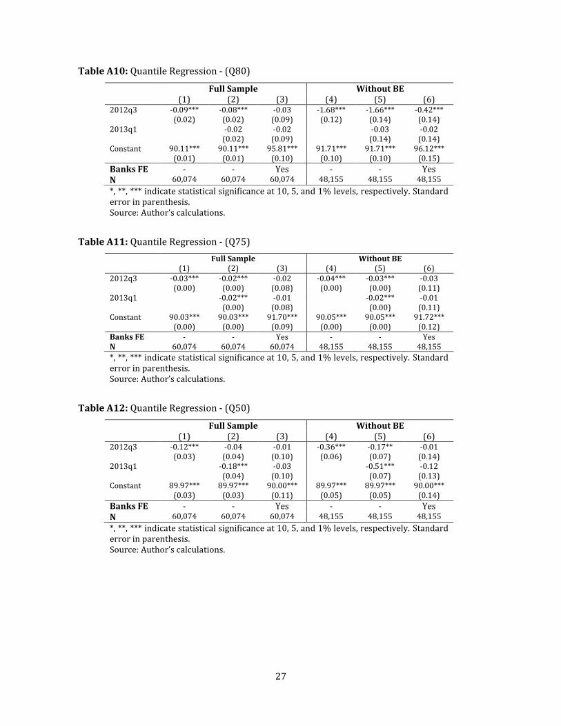
Table A10: Quantile Regression - (Q80)
Full Sample Without BE (1) (2) (3) (4) (5) (6) 2012q3 -0.09*** -0.08*** -0.03 -1.68*** -1.66*** -0.42*** (0.02) (0.02) (0.09) (0.12) (0.14) (0.14) 2013q1 -0.02 -0.02 -0.03 -0.02 (0.02) (0.09) (0.14) (0.14) Constant 90.11*** 90.11*** 95.81*** 91.71*** 91.71*** 96.12*** (0.01) (0.01) (0.10) (0.10) (0.10) (0.15)
Banks FE - - Yes - - Yes N 60,074 60,074 60,074 48,155 48,155 48,155
*, **, *** indicate statistical significance at 10, 5, and 1% levels, respectively. Standard error in parenthesis. Source: Author’s calculations.
Table A11: Quantile Regression - (Q75)
Full Sample Without BE (1) (2) (3) (4) (5) (6) 2012q3 -0.03*** -0.02*** -0.02 -0.04*** -0.03*** -0.03 (0.00) (0.00) (0.08) (0.00) (0.00) (0.11) 2013q1 -0.02*** -0.01 -0.02*** -0.01 (0.00) (0.08) (0.00) (0.11) Constant 90.03*** 90.03*** 91.70*** 90.05*** 90.05*** 91.72*** (0.00) (0.00) (0.09) (0.00) (0.00) (0.12) Banks FE - - Yes - - Yes N 60,074 60,074 60,074 48,155 48,155 48,155
*, **, *** indicate statistical significance at 10, 5, and 1% levels, respectively. Standard error in parenthesis. Source: Author’s calculations.
Table A12: Quantile Regression - (Q50)
Full Sample Without BE (1) (2) (3) (4) (5) (6) 2012q3 -0.12*** -0.04 -0.01 -0.36*** -0.17** -0.01 (0.03) (0.04) (0.10) (0.06) (0.07) (0.14) 2013q1 -0.18*** -0.03 -0.51*** -0.12 (0.04) (0.10) (0.07) (0.13) Constant 89.97*** 89.97*** 90.00*** 89.97*** 89.97*** 90.00*** (0.03) (0.03) (0.11) (0.05) (0.05) (0.14)
Banks FE - - Yes - - Yes N 60,074 60,074 60,074 48,155 48,155 48,155
*, **, *** indicate statistical significance at 10, 5, and 1% levels, respectively. Standard error in parenthesis. Source: Author’s calculations.

28
Week and tighter window
Table A13: Quantile Regression - (Q90)
Full Sample Without BE (1) (2) (3) (4) (5) (6) 2012-18-06 -7.37*** -4.97*** 0.00 -5.00*** -2.33*** 0.00 (0.44) (0.10) (0.18) (0.06) (0.36) (0.18) 2012-18-12 -4.93*** -0.07 -6.81*** -3.24*** (0.09) (0.15) (0.31) (0.15) Constant 100.00*** 100.00*** 100.00*** 100.00*** 100.00*** 100.00*** (0.39) (0.08) (0.20) (0.05) (0.28) (0.18)
Banks FE - - Yes - - Yes N 60,074 60,074 60,074 48,155 48,155 48,155
*, **, *** indicate statistical significance at 10, 5, and 1% levels, respectively. Standard error in parenthesis. Source: Author’s calculations.
Table A14: Quantile Regression - (Q85)
Full Sample Without BE (1) (2) (3) (4) (5) (6) 2012-18-06 -4.94*** -4.46*** -0.14** -6.72*** -3.89*** -0.96*** (0.04) (0.13) (0.07) (0.23) (0.35) (0.14) 2012-18-12 -0.50*** -0.04 -3.03*** -0.80*** (0.11) (0.06) (0.30) (0.12) Constant 95.00*** 95.00*** 100.00*** 96.95*** 96.95*** 100.00*** (0.04) (0.11) (0.07) (0.20) (0.28) (0.14)
Banks FE - - Yes - - Yes N 60,074 60,074 60,074 48,155 48,155 48,155
*, **, *** indicate statistical significance at 10, 5, and 1% levels, respectively. Standard error in parenthesis. Source: Author’s calculations.

29
Table A15: Quantile Regression - (Q80)
Full Sample Without BE (1) (2) (3) (4) (5) (6) 2012-18-06 -0.21*** -0.19*** -0.03 -2.08*** -2.04*** -0.68*** (0.03) (0.03) (0.10) (0.11) (0.14) (0.15) 2012-18-12 -0.02 -0.02 -0.05 -0.02 (0.02) (0.09) (0.12) (0.13) Constant 90.24*** 90.24*** 95.81*** 92.11*** 92.11*** 96.33*** (0.02) (0.02) (0.11) (0.10) (0.11) (0.15)
Banks FE - - Yes - - Yes N 60,074 60,074 60,074 48,155 48,155 48,155
*, **, *** indicate statistical significance at 10, 5, and 1% levels, respectively. Standard error in parenthesis. Source: Author’s calculations.
Table A16: Quantile Regression - (Q75)
Full Sample Without BE (1) (2) (3) (4) (5) (6) 2012-18-06 -0.03*** -0.02*** -0.02 -0.05*** -0.03*** -0.03 (0.00) (0.00) (0.09) (0.01) (0.01) (0.12) 2012-18-12 -0.02*** -0.01 -0.02*** -0.01 (0.00) (0.08) (0.01) (0.11) Constant 90.04*** 90.04*** 91.70*** 90.05*** 90.05*** 91.71*** (0.00) (0.00) (0.10) (0.01) (0.01) (0.13)
Banks FE - - Yes - - Yes N 60,074 60,074 60,074 48,155 48,155 48,155
*, **, *** indicate statistical significance at 10, 5, and 1% levels, respectively. Standard error in parenthesis. Source: Author’s calculations.
Table A17: Quantile Regression - (Q50)
Full Sample Without BE (1) (2) (3) (4) (5) (6) 2012-18-06 -0.08** -0.03 -0.00 -0.28*** -0.11 -0.01 (0.03) (0.04) (0.11) (0.07) (0.07) (0.15) 2012-18-12 -0.14*** -0.02 -0.43*** -0.05 (0.03) (0.09) (0.06) (0.13) Constant 89.97*** 89.97*** 90.00*** 89.97*** 89.97*** 90.00*** (0.03) (0.03) (0.12) (0.06) (0.06) (0.15)
Banks FE - - Yes - - Yes N 60,074 60,074 60,074 48,155 48,155 48,155
*, **, *** indicate statistical significance at 10, 5, and 1% levels, respectively. Standard error in parenthesis. Source: Author’s calculations.

DOCUMENTOS DE TRABAJO • Febrero 2017