Documentation for the VS-Lite Model, version 2.2

S.E. Tolwinski-Ward (tolwinski@math.arizona.edu)

November 22, 2011

1 New Features and Relation to Past Model Versions

There is one new features of the VS-Lite model in version 2.2: the option to run the “Leaky Bucket”

hydrology at a sub-monthly timestep (hereafter referred to as “substepping”). The model may be

run without the substepping option, in which case it is equivalent to the VS-Lite model version 2.1

previously archived on the WDCA-Paleo software library

(http://www.ncdc.noaa.gov/paleo/softlib/softlib.html). As with previous versions, VS-Lite version

2.2 is also compatible with the freeware Matlab-clone, Octave 3.2.4 s(www.octave.org).

The original Leaky Bucket model of hydrology requires monthly input climate data, but actually

updates soil moisture at a sub-monthly timestep to account for the nonlinearity of the soil moisture

response (Huang et al. (1996)). Without the substepping, the Leaky Bucket model authors found

that a single step for the entire month can cause the soil to dry out too quickly (Nicholas Graham,

Konstantine Georgakakos, personal communication, March 2011.) Past versions of the VS-Lite

model code did not include the option for sub-stepping. Version 2.2 with the substepping option

bases tree-ring width growth on the instantaneous soil moisture computed at the end of each

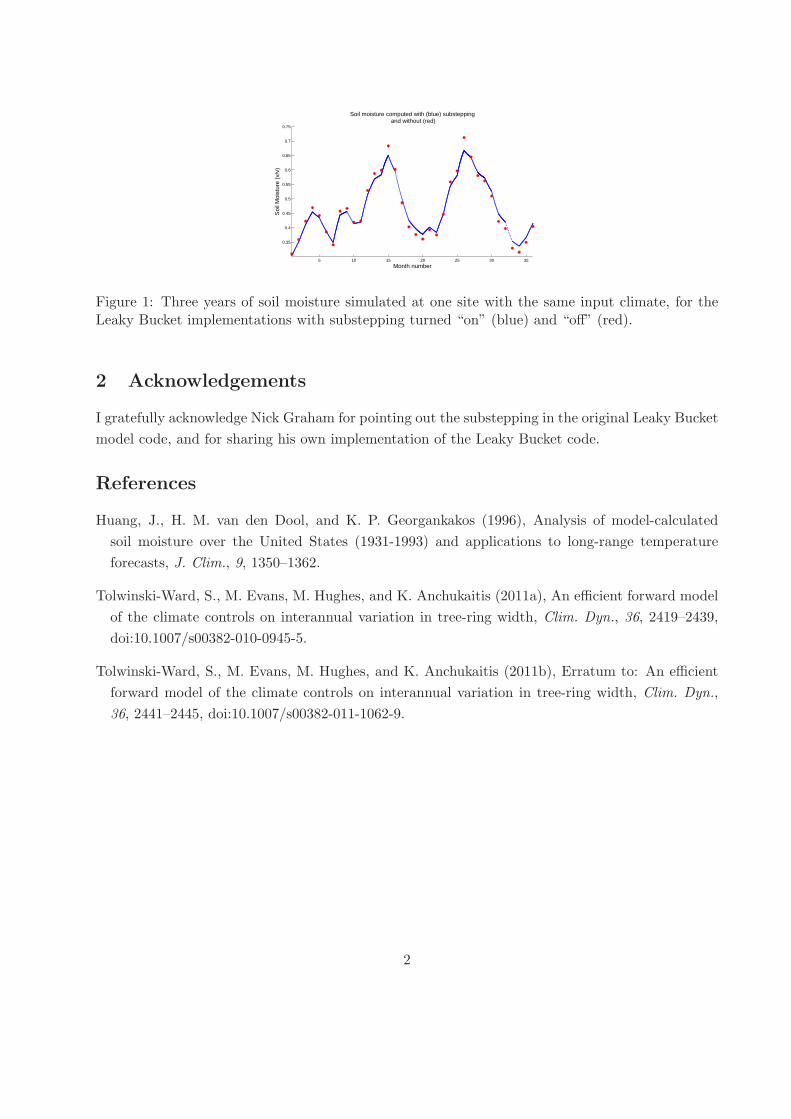
month. In general, comparisons of the model output with and without substepping show that using

substepping tends to add more “drag” to the modeled hydrological system, so that the substepping

tends to curb the largest rates of change in the system compared to the implementation without

substepping (see Figure 1). Note that if the initial soil moisture input to the model is less than

zero and thus unphysical, the model sets the initial value to a default value of 0.2 v/v.

The VS-lite v2.2 model has been validated with leaky bucket temporal substepping using all the

same tests used and described and implemented by Tolwinski-Ward et al. (2011a) and Tolwinski-

Ward et al. (2011b) to validate the earlier model version. The differences in simulations performed

with and without substepping appear quite minor in the test networks examined; results are pro-

vided Tables 3-6 and Figures 2-12 below (Tables and Figures are numbered to correspond with

numbering of results in Tolwinski-Ward et al. (2011a)).

A script called vslite bayes param cal.m for Bayesian calibration of the VS-Lite v2.2 model

parameters has also been developed and archived with separate documentation at the WDCA-

Paleo software library (http://www.ncdc.noaa.gov/paleo/softlib/softlib.html).

1

5 10 15 20 25 30 35

0.35

0.4

0.45

0.5

0.55

0.6

0.65

0.7

0.75

Month number

Soi

l Moi

stur

e (v

/v)

Soil moisture computed with (blue) substepping and without (red)

Figure 1: Three years of soil moisture simulated at one site with the same input climate, for theLeaky Bucket implementations with substepping turned “on” (blue) and “off” (red).

2 Acknowledgements

I gratefully acknowledge Nick Graham for pointing out the substepping in the original Leaky Bucket

model code, and for sharing his own implementation of the Leaky Bucket code.

References

Huang, J., H. M. van den Dool, and K. P. Georgankakos (1996), Analysis of model-calculated

soil moisture over the United States (1931-1993) and applications to long-range temperature

forecasts, J. Clim., 9, 1350–1362.

Tolwinski-Ward, S., M. Evans, M. Hughes, and K. Anchukaitis (2011a), An efficient forward model

of the climate controls on interannual variation in tree-ring width, Clim. Dyn., 36, 2419–2439,

doi:10.1007/s00382-010-0945-5.

Tolwinski-Ward, S., M. Evans, M. Hughes, and K. Anchukaitis (2011b), Erratum to: An efficient

forward model of the climate controls on interannual variation in tree-ring width, Clim. Dyn.,

36, 2441–2445, doi:10.1007/s00382-011-1062-9.

2

Table 2: Fraction of observed signal variances at frequencies of 1/5 yr−1 and lower at each site; cor-relation and significance of bristlecone pine simulations with observed chronologies. Low-frequencysignals are given by 5-year filtering of the signals; high-frequency signals are the residuals. Low-freq. p-values are corrected for effective number of degrees of freedom. Sites marked “UFB” are atthe upper forest border. Highlighted rows are results for VS-Lite v2.2 with substepping

turned “on”, while white rows are previous results for simulations with VS-Lite v2.1.

Site Abbrv. Low Freq. Var. Frac. Low-freq. High-freq.

Pearl Peak (UFB) PRL 0.64 0.55 (p < 0.01) 0.12 (p ≈ 0.3)

Pearl Peak (UFB) PRL 0.64 0.57 (p < 0.01) 0.10 (p ≈ 0.3)

Sheep Mountain (UFB) SHP 0.48 0.69 (p < 0.001) 0.31 (p < 0.002)

Sheep Mountain (UFB) SHP 0.48 0.69 (p < 0.001) 0.31 (p < 0.002)

Mount Washington (UFB) MWA 0.51 0.51 (p < 0.02) 0.12 (p ≈ 0.2)

Mount Washington (UFB) MWA 0.51 0.49 (p < 0.03) 0.16 (p ≈ 0.1)

Cottonwood Lower CWL 0.60 0.21 (p ≈ 0.3) 0.35 (p < 0.001)

Cottonwood Lower CWL 0.60 0.21 (p ≈ 0.3) 0.34 (p < 0.001)

Methuselah Walk MWK 0.45 0.42 (p ≈ 0.06) 0.32 (p < 0.002)

Methuselah Walk MWK 0.45 0.42 (p ≈ 0.06) 0.29 (p < 0.01)

Patriarch Lower PAL 0.55 0.08 (p ≈ 0.7) 0.28 (p < 0.01)

Patriarch Lower PAL 0.55 0.09 (p ≈ 0.7) 0.25 (p < 0.01)

Table 3: Mean percentage of sites, across an ensemble of 100 simulations, whose simulations cor-relate significantly with observed tree-ring width chronologies at two significance levels in the M08network. Results shown for simulations by principal components regression calibrated at each site,simulations by VS-Lite with parameters calibrated at each site, and simulations by VS-lite with asingle, “global” parameter set calibrated on the network as a whole. Errors represent 1 standarddeviation in the percentages simulated significantly across ensemble members. Highlighted rows

are results for simulations using VS-Lite v2.2 with substepping turned “on”, and white

rows show previous results with VS-Lite v2.1.

M08 Network (N = 282)

PC Regr., site-by-site VS-Lite, site-by-site VS-Lite, global

Calibration Validation Calibration Validation Calibration Validation

p < 0.01 73% ± 3% 40% ± 3% 69% ± 2% 59% ± 3% 46% ± 3% 48% ± 3%

p < 0.01 73% ± 3% 40% ± 3% 69% ± 2% 60% ± 3% 47% ± 2% 49% ± 3%

p < 0.05 83% ± 3% 56% ± 3% 80% ± 2% 71% ± 3% 59% ± 3% 61% ± 3%

p < 0.05 83% ± 3% 56% ± 3% 80% ± 2% 71% ± 3% 59% ± 2% 61% ± 3%

3

1900 1910 1920 1930 1940 1950 1960 1970 1980 1990 2000−4

−2

0

2

4VS−Lite at PRL, r = 0.39

1900 1910 1920 1930 1940 1950 1960 1970 1980 1990 2000−4

−2

0

2

4VS−Lite at SHP, r = 0.54

1900 1910 1920 1930 1940 1950 1960 1970 1980 1990 2000−4

−2

0

2

4VS−Lite at MWA, r = 0.39

1900 1910 1920 1930 1940 1950 1960 1970 1980 1990 2000−4

−2

0

2

4VS−Lite at CWL, r = 0.3

1900 1910 1920 1930 1940 1950 1960 1970 1980 1990−4

−2

0

2

4VS−Lite at MWK, r = 0.42

1900 1910 1920 1930 1940 1950 1960 1970 1980 1990 2000−4

−2

0

2

4VS−Lite at PAL, r = 0.19

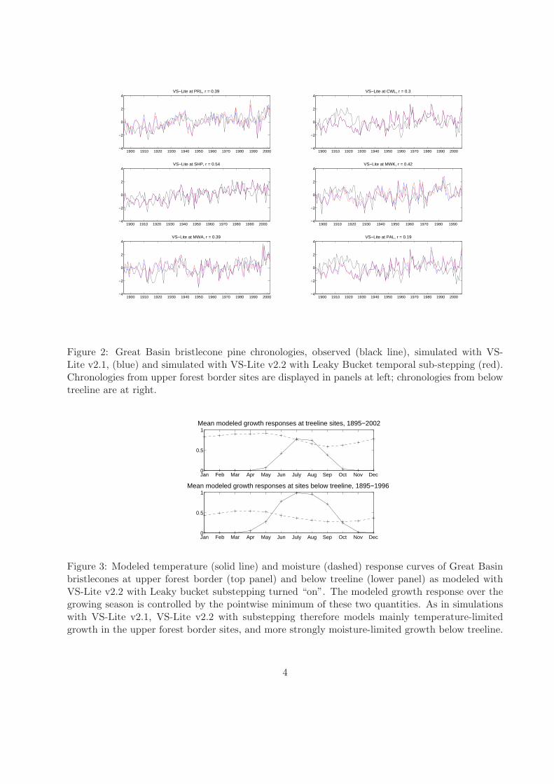
Figure 2: Great Basin bristlecone pine chronologies, observed (black line), simulated with VS-Lite v2.1, (blue) and simulated with VS-Lite v2.2 with Leaky Bucket temporal sub-stepping (red).Chronologies from upper forest border sites are displayed in panels at left; chronologies from belowtreeline are at right.

Jan Feb Mar Apr May Jun July Aug Sep Oct Nov Dec0

0.5

1Mean modeled growth responses at treeline sites, 1895−2002

Jan Feb Mar Apr May Jun July Aug Sep Oct Nov Dec0

0.5

1Mean modeled growth responses at sites below treeline, 1895−1996

Figure 3: Modeled temperature (solid line) and moisture (dashed) response curves of Great Basinbristlecones at upper forest border (top panel) and below treeline (lower panel) as modeled withVS-Lite v2.2 with Leaky bucket substepping turned “on”. The modeled growth response over thegrowing season is controlled by the pointwise minimum of these two quantities. As in simulationswith VS-Lite v2.1, VS-Lite v2.2 with substepping therefore models mainly temperature-limitedgrowth in the upper forest border sites, and more strongly moisture-limited growth below treeline.

4

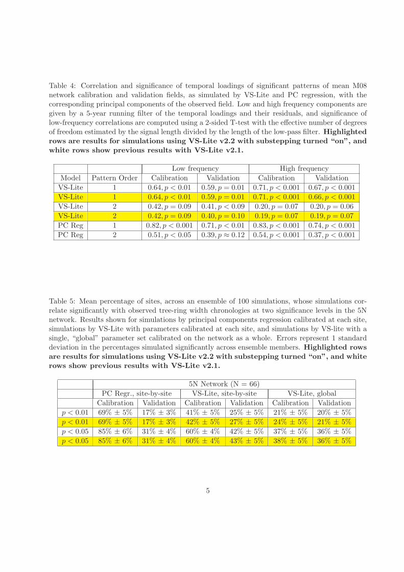
Table 4: Correlation and significance of temporal loadings of significant patterns of mean M08network calibration and validation fields, as simulated by VS-Lite and PC regression, with thecorresponding principal components of the observed field. Low and high frequency components aregiven by a 5-year running filter of the temporal loadings and their residuals, and significance oflow-frequency correlations are computed using a 2-sided T-test with the effective number of degreesof freedom estimated by the signal length divided by the length of the low-pass filter. Highlighted

rows are results for simulations using VS-Lite v2.2 with substepping turned “on”, and

white rows show previous results with VS-Lite v2.1.

Low frequency High frequency

Model Pattern Order Calibration Validation Calibration Validation

VS-Lite 1 0.64, p < 0.01 0.59, p = 0.01 0.71, p < 0.001 0.67, p < 0.001

VS-Lite 1 0.64, p < 0.01 0.59, p = 0.01 0.71, p < 0.001 0.66, p < 0.001

VS-Lite 2 0.42, p = 0.09 0.41, p < 0.09 0.20, p = 0.07 0.20, p = 0.06

VS-Lite 2 0.42, p = 0.09 0.40, p = 0.10 0.19, p = 0.07 0.19, p = 0.07

PC Reg 1 0.82, p < 0.001 0.71, p < 0.01 0.83, p < 0.001 0.74, p < 0.001

PC Reg 2 0.51, p < 0.05 0.39, p ≈ 0.12 0.54, p < 0.001 0.37, p < 0.001

Table 5: Mean percentage of sites, across an ensemble of 100 simulations, whose simulations cor-relate significantly with observed tree-ring width chronologies at two significance levels in the 5Nnetwork. Results shown for simulations by principal components regression calibrated at each site,simulations by VS-Lite with parameters calibrated at each site, and simulations by VS-lite with asingle, “global” parameter set calibrated on the network as a whole. Errors represent 1 standarddeviation in the percentages simulated significantly across ensemble members. Highlighted rows

are results for simulations using VS-Lite v2.2 with substepping turned “on”, and white

rows show previous results with VS-Lite v2.1.

5N Network (N = 66)

PC Regr., site-by-site VS-Lite, site-by-site VS-Lite, global

Calibration Validation Calibration Validation Calibration Validation

p < 0.01 69% ± 5% 17% ± 3% 41% ± 5% 25% ± 5% 21% ± 5% 20% ± 5%

p < 0.01 69% ± 5% 17% ± 3% 42% ± 5% 27% ± 5% 24% ± 5% 21% ± 5%

p < 0.05 85% ± 6% 31% ± 4% 60% ± 4% 42% ± 5% 37% ± 5% 36% ± 5%

p < 0.05 85% ± 6% 31% ± 4% 60% ± 4% 43% ± 5% 38% ± 5% 36% ± 5%

5

VS−Lite,Calibration

120 ° W 110° W 100° W 90° W 80

° W 70

° W

30 ° N

40 ° N

50 ° N

VS−Lite,Validation

120 ° W 110° W 100° W 90° W 80

° W 70

° W

30 ° N

40 ° N

50 ° N

PC Regression,Calibration

120 ° W 110° W 100° W 90° W 80

° W 70

° W

30 ° N

40 ° N

50 ° N

PC Regression,Validation

120 ° W 110° W 100° W 90° W 80

° W 70

° W

30 ° N

40 ° N

50 ° N

Figure 4a: Mean validation-interval significance of correlations of ring width simulations withobservations over a 100-member ensemble of simulations of the M08 network, simulated with VS-lite v2.2 with substepping turned “on”. Ensemble members differ in their randomized calibrationintervals. Black circles: p < .01, gray circles: p < .05, white circles: p > .05.

6

VSLite Validationno substepping

120 ° W 110° W 100° W 90° W 80° W

70° W

30 ° N

40 ° N

50 ° N

VSLite Validationwith substepping

120 ° W 110° W 100° W 90° W 80° W

70° W

30 ° N

40 ° N

50 ° N

Figure 4b: Mean validation-interval significance of correlations of ring width simulations withobservations over a 100-member ensemble of simulations of the M08 network, simulated with VS-lite v2.1 (left) and v2.2 with substepping turned “on” (right). Ensemble members differ in theirrandomized calibration intervals. Black circles: p < .01, gray circles: p < .05, white circles: p > .05.

0.02 0.04 0.06 0.08 0.1

0.35

0.4

0.45

0.5

0.55

0.6

0.65

0.7

0.75

0.8

p−value

Fra

ctio

n si

gnifi

cant

Fraction of M08 simulationssignificantly correlated with observation

0.4 0.6 0.8 10.4

0.5

0.6

0.7

0.8

0.9

1

Stability index of statistical model

Sta

bilit

y in

dex

of V

SLi

te m

odel

Stability index of models,M08 Network Sites

VSLite v2.1

VSLite v2.1 global

VSLite v3.0

VSLite v3.0 global

PC Reg.

Figure 5: Performance indices of modeling by VS-Lite and principal components regression on theM08 Network. Left panel plots the fraction of network sites whose simulations correlate significantlywith observations at a range of p-values for three different simulation approaches. Previous resultsare plotted in black for comparison; results for simulations using VS-Lite v2.2 with substeppingturned “on” are plotted in red. Right panel plots the stability index (eqn. 3) of simulations bycorrected VS-Lite code versus PC regression, with one indicating perfect stability of simulationsfrom the calibration to validation periods, and zero representing complete instability. 203 out of282 points fall above y = x (compare to 202 out of 282 for simulations using VS-lite v2.1).

7

First EOF,Observed

120 ° W 110° W 100° W 90° W 80° W 70

° W

30 ° N

40 ° N

50 ° N

First EOF,Simulated

120 ° W 110° W 100° W 90° W 80° W 70

° W

30 ° N

40 ° N

50 ° N

1900 1910 1920 1930 1940 1950 1960 1970 1980−0.4

−0.3

−0.2

−0.1

0

0.1

0.2

0.3

Year

Observed (dashed) and MVF (solid) PC 1, r = 0.62

1 2 3 4 5 6 7 8 9 10 11 12

Projected gT (solid) and g

W (dashed)

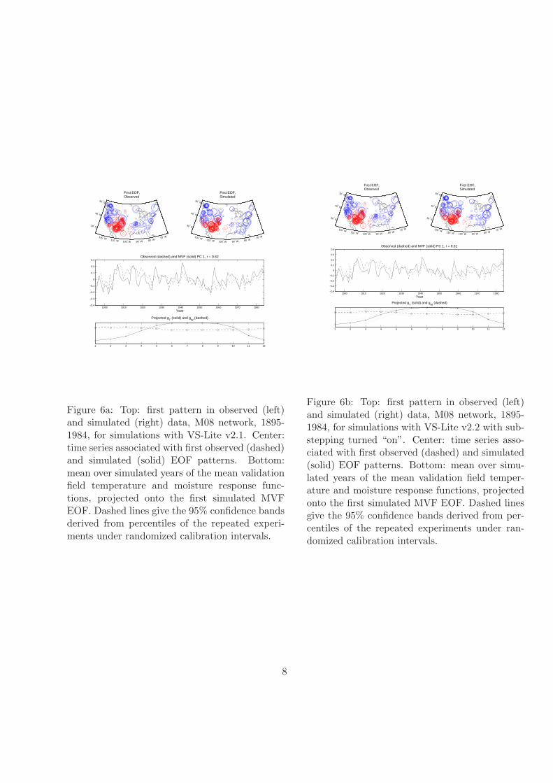
Figure 6a: Top: first pattern in observed (left)and simulated (right) data, M08 network, 1895-1984, for simulations with VS-Lite v2.1. Center:time series associated with first observed (dashed)and simulated (solid) EOF patterns. Bottom:mean over simulated years of the mean validationfield temperature and moisture response func-tions, projected onto the first simulated MVFEOF. Dashed lines give the 95% confidence bandsderived from percentiles of the repeated experi-ments under randomized calibration intervals.

First EOF,Observed

120 ° W 110° W 100° W 90° W 80° W 70

° W

30 ° N

40 ° N

50 ° N

First EOF,Simulated

120 ° W 110° W 100° W 90° W 80° W 70

° W

30 ° N

40 ° N

50 ° N

1900 1910 1920 1930 1940 1950 1960 1970 1980−0.4

−0.3

−0.2

−0.1

0

0.1

0.2

0.3

0.4

Year

Observed (dashed) and MVF (solid) PC 1, r = 0.61

1 2 3 4 5 6 7 8 9 10 11 12

Projected gT (solid) and g

W (dashed)

Figure 6b: Top: first pattern in observed (left)and simulated (right) data, M08 network, 1895-1984, for simulations with VS-Lite v2.2 with sub-stepping turned “on”. Center: time series asso-ciated with first observed (dashed) and simulated(solid) EOF patterns. Bottom: mean over simu-lated years of the mean validation field temper-ature and moisture response functions, projectedonto the first simulated MVF EOF. Dashed linesgive the 95% confidence bands derived from per-centiles of the repeated experiments under ran-domized calibration intervals.

8

Second EOF,Observed

120 ° W 110° W 100° W 90° W 80° W 70

° W

30 ° N

40 ° N

50 ° N

Second EOF,Simulated

120 ° W 110° W 100° W 90° W 80° W 70

° W

30 ° N

40 ° N

50 ° N

1900 1910 1920 1930 1940 1950 1960 1970 1980−0.4

−0.3

−0.2

−0.1

0

0.1

0.2

0.3

Year

Observed (dashed) and MVF (solid) PC 2, r = 0.33

1 2 3 4 5 6 7 8 9 10 11 12

Projected gT (solid) and g

W (dashed)

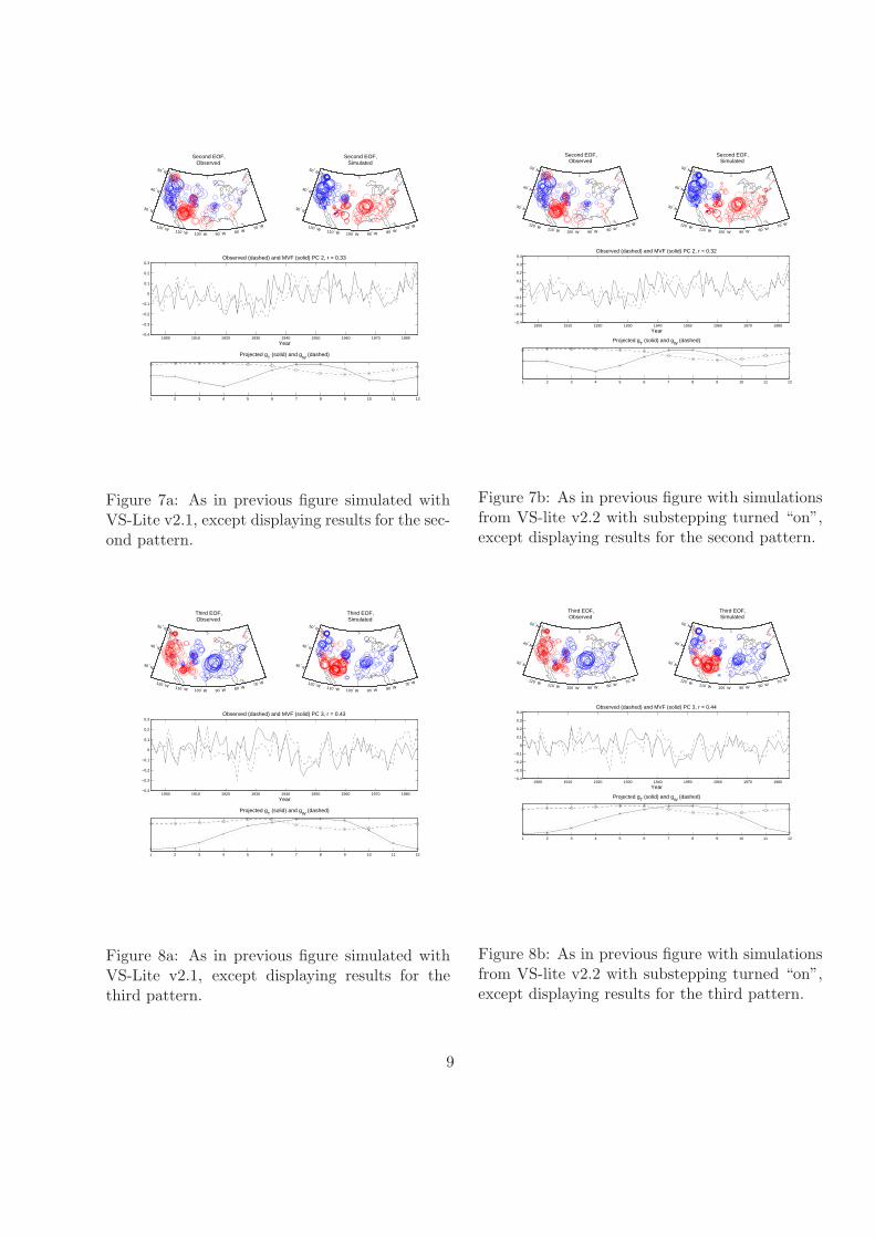
Figure 7a: As in previous figure simulated withVS-Lite v2.1, except displaying results for the sec-ond pattern.

Second EOF,Observed

120 ° W 110° W 100° W 90° W 80° W 70

° W

30 ° N

40 ° N

50 ° N

Second EOF,Simulated

120 ° W 110° W 100° W 90° W 80° W 70

° W

30 ° N

40 ° N

50 ° N

1900 1910 1920 1930 1940 1950 1960 1970 1980−0.4

−0.3

−0.2

−0.1

0

0.1

0.2

0.3

0.4

Year

Observed (dashed) and MVF (solid) PC 2, r = 0.32

1 2 3 4 5 6 7 8 9 10 11 12

Projected gT (solid) and g

W (dashed)

Figure 7b: As in previous figure with simulationsfrom VS-lite v2.2 with substepping turned “on”,except displaying results for the second pattern.

Third EOF,Observed

120 ° W 110° W 100° W 90° W 80° W 70

° W

30 ° N

40 ° N

50 ° N

Third EOF,Simulated

120 ° W 110° W 100° W 90° W 80° W 70

° W

30 ° N

40 ° N

50 ° N

1900 1910 1920 1930 1940 1950 1960 1970 1980−0.4

−0.3

−0.2

−0.1

0

0.1

0.2

0.3

Year

Observed (dashed) and MVF (solid) PC 3, r = 0.43

1 2 3 4 5 6 7 8 9 10 11 12

Projected gT (solid) and g

W (dashed)

Figure 8a: As in previous figure simulated withVS-Lite v2.1, except displaying results for thethird pattern.

Third EOF,Observed

120 ° W 110° W 100° W 90° W 80° W 70

° W

30 ° N

40 ° N

50 ° N

Third EOF,Simulated

120 ° W 110° W 100° W 90° W 80° W 70

° W

30 ° N

40 ° N

50 ° N

1900 1910 1920 1930 1940 1950 1960 1970 1980−0.4

−0.3

−0.2

−0.1

0

0.1

0.2

0.3

0.4

Year

Observed (dashed) and MVF (solid) PC 3, r = 0.44

1 2 3 4 5 6 7 8 9 10 11 12

Projected gT (solid) and g

W (dashed)

Figure 8b: As in previous figure with simulationsfrom VS-lite v2.2 with substepping turned “on”,except displaying results for the third pattern.

9

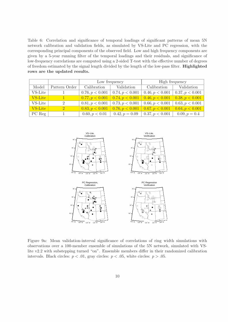
Table 6: Correlation and significance of temporal loadings of significant patterns of mean 5Nnetwork calibration and validation fields, as simulated by VS-Lite and PC regression, with thecorresponding principal components of the observed field. Low and high frequency components aregiven by a 5-year running filter of the temporal loadings and their residuals, and significance oflow-frequency correlations are computed using a 2-sided T-test with the effective number of degreesof freedom estimated by the signal length divided by the length of the low-pass filter. Highlighted

rows are the updated results.

Low frequency High frequency

Model Pattern Order Calibration Validation Calibration Validation

VS-Lite 1 0.76, p < 0.001 0.74, p < 0.001 0.46, p < 0.001 0.37, p < 0.001

VS-Lite 1 0.77, p < 0.001 0.74, p < 0.001 0.46, p < 0.001 0.38, p < 0.001

VS-Lite 2 0.81, p < 0.001 0.73, p < 0.001 0.66, p < 0.001 0.63, p < 0.001

VS-Lite 2 0.83, p < 0.001 0.76, p < 0.001 0.67, p < 0.001 0.64, p < 0.001

PC Reg 1 0.60, p < 0.01 0.42, p = 0.09 0.37, p < 0.001 0.09, p = 0.4

VS−Lite,Calibration

125° W 120° W 115° W 110° W 105° W

35° N

40° N

45° N

50° N

VS−Lite,Verification

125° W 120° W 115° W 110° W 105° W

35° N

40° N

45° N

50° N

PC Regression,Calibration

125° W 120° W 115° W 110° W 105° W

35° N

40° N

45° N

50° N

PC RegressionVerification

125° W 120° W 115° W 110° W 105° W

35° N

40° N

45° N

50° N

Figure 9a: Mean validation-interval significance of correlations of ring width simulations withobservations over a 100-member ensemble of simulations of the 5N network, simulated with VS-lite v2.2 with substepping turned “on”. Ensemble members differ in their randomized calibrationintervals. Black circles: p < .01, gray circles: p < .05, white circles: p > .05.

10

VS−Lite Validationno substepping

125° W 120° W 115° W 110° W 105° W

35° N

40° N

45° N

50° N

VS−Lite Validationwith substepping

125° W 120° W 115° W 110° W 105° W

35° N

40° N

45° N

50° N

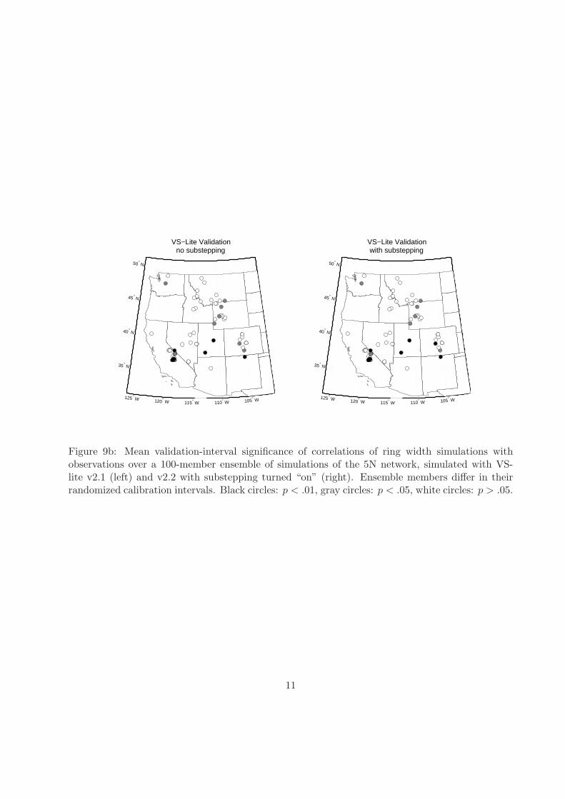
Figure 9b: Mean validation-interval significance of correlations of ring width simulations withobservations over a 100-member ensemble of simulations of the 5N network, simulated with VS-lite v2.1 (left) and v2.2 with substepping turned “on” (right). Ensemble members differ in theirrandomized calibration intervals. Black circles: p < .01, gray circles: p < .05, white circles: p > .05.

11

0.02 0.04 0.06 0.08 0.1

0.2

0.25

0.3

0.35

0.4

0.45

0.5

0.55

p−value

Fra

ctio

n si

gnifi

cant

Fraction of 5N network simulationssignificantly correlated with observation

0.4 0.5 0.6 0.7 0.8 0.9 10.4

0.5

0.6

0.7

0.8

0.9

1

Stability index of statistical model

Sta

bilit

y in

dex

of V

SLi

te m

odel

Stability index of models,5N Network Sites

VSLite v2.1

VSLite v2.1, global

VSlite v3.0

VSlite v3.0, global

PC Reg.

Figure 10: Performance indices of modeling by VS-Lite and principal components regression on the5N network. Left panel plots the fraction of network sites whose simulations correlate significantlywith observations at a range of p-values for three different simulation approaches. Previous resultsare plotted in black for comparison; results for simulations using VS-Lite v2.2 with substeppingturned “on” are plotted in red. Right panel plots the stability index (eqn. 3) of simulations bycorrected VS-Lite code versus PC regression, with one indicating perfect stability of simulationsfrom the calibration to validation periods, and zero representing complete instability. 48 out of 66points fall above x = y (compare to 42 out of 66 with previous results using VS-Lite v2.1).

12

First EOF,Observed Chronologies

125° W 120° W 115° W 110° W 105° W

35° N

40° N

45° N

50° N

1st Heterogeneous Corr. Map,Simulated RWs

125° W 120° W 115° W 110° W 105° W

35° N

40° N

45° N

50° N

1900 1910 1920 1930 1940 1950 1960 1970 1980−3

−2

−1

0

1

2

3

Year

Observed PC 1 (dashed) and first MVF time series (solid)r = 0.59

1 2 3 4 5 6 7 8 9 10 11 120

0.5

1

Projected gT (solid) and g

W (dashed)

Month

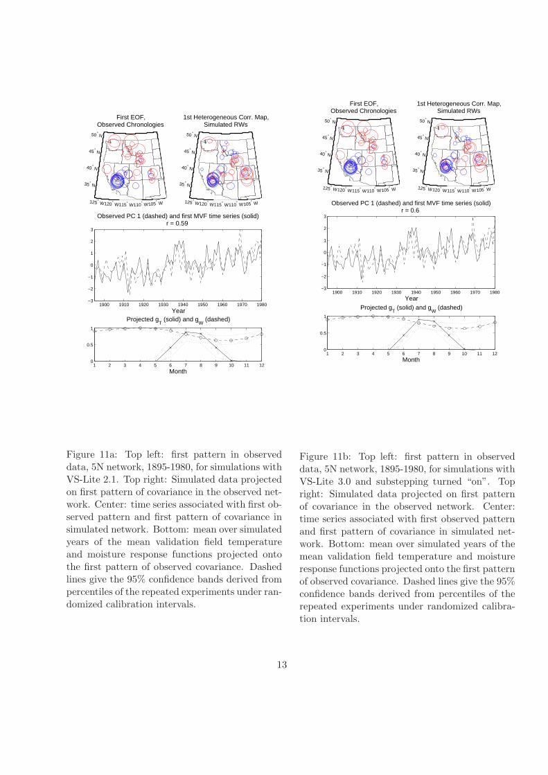
Figure 11a: Top left: first pattern in observeddata, 5N network, 1895-1980, for simulations withVS-Lite 2.1. Top right: Simulated data projectedon first pattern of covariance in the observed net-work. Center: time series associated with first ob-served pattern and first pattern of covariance insimulated network. Bottom: mean over simulatedyears of the mean validation field temperatureand moisture response functions projected ontothe first pattern of observed covariance. Dashedlines give the 95% confidence bands derived frompercentiles of the repeated experiments under ran-domized calibration intervals.

First EOF,Observed Chronologies

125° W 120° W 115° W 110° W 105° W

35° N

40° N

45° N

50° N

1st Heterogeneous Corr. Map,Simulated RWs

125° W 120° W 115° W 110° W 105° W

35° N

40° N

45° N

50° N

1900 1910 1920 1930 1940 1950 1960 1970 1980−3

−2

−1

0

1

2

3

Year

Observed PC 1 (dashed) and first MVF time series (solid)r = 0.6

1 2 3 4 5 6 7 8 9 10 11 120

0.5

1

Projected gT (solid) and g

W (dashed)

Month

Figure 11b: Top left: first pattern in observeddata, 5N network, 1895-1980, for simulations withVS-Lite 3.0 and substepping turned “on”. Topright: Simulated data projected on first patternof covariance in the observed network. Center:time series associated with first observed patternand first pattern of covariance in simulated net-work. Bottom: mean over simulated years of themean validation field temperature and moistureresponse functions projected onto the first patternof observed covariance. Dashed lines give the 95%confidence bands derived from percentiles of therepeated experiments under randomized calibra-tion intervals.

13

Second EOFObserved Chronologies

125° W 120° W 115° W 110° W 105° W

35° N

40° N

45° N

50° N

2nd Heterogeneous Corr. Map,Simulated RWs

125° W 120° W 115° W 110° W 105° W

35° N

40° N

45° N

50° N

1900 1910 1920 1930 1940 1950 1960 1970 1980−3

−2

−1

0

1

2

3

Year

Observed PC 2 (dashed) and 2nd MVF time series (solid)r = 0.68

1 2 3 4 5 6 7 8 9 10 11 120

0.5

1

Projected gT (solid) and g

W (dashed)

Month

Figure 12a: As in previous figure with simulationsfrom VS-Lite v2.1, except displaying results forthe second pattern.

Second EOFObserved Chronologies

125° W 120° W 115° W 110° W 105° W

35° N

40° N

45° N

50° N

2nd Heterogeneous Corr. Map,Simulated RWs

125° W 120° W 115° W 110° W 105° W

35° N

40° N

45° N

50° N

1900 1910 1920 1930 1940 1950 1960 1970 1980−3

−2

−1

0

1

2

3

Year

Observed PC 2 (dashed) and 2nd MVF time series (solid)r = 0.7

1 2 3 4 5 6 7 8 9 10 11 120

0.5

1

Projected gT (solid) and g

W (dashed)

Month

Figure 12b: As in previous figure with simulationsfrom VS-Lite v2.2 with substepping turned “on”,except displaying results for the second pattern.

14