Babes–Bolyai University of Cluj-NapocaFaculty of Mathematics and Informatics

Department of Applied Mathematics

Doctoral Report

Scientific conductor: PhD student:Dr. Ioan A. Rus Egri Edith

2006

Numerical and approximativemethods in some mathematical

models

Universitatea Babes–Bolyai, Cluj-NapocaFacultatea de Matematica si Informatica

Matematica Aplicata

Referat de doctorat

Conducator stiintific, Doctorand,Prof. dr. Ioan A. Rus Egri Edith

2006

Metode numerice si aproximative ınunele modele matematice

Contents

1 Introduction 2

2 The computational singular perturbation method 32.1 The theory of CSP . . . . . . . . . . . . . . . . . . . . . . . . . . . . . . . 42.2 A simple example . . . . . . . . . . . . . . . . . . . . . . . . . . . . . . . . 6

3 Euler method 8

4 Runge-Kutta methods 104.1 Runge-Kutta method of order 2 . . . . . . . . . . . . . . . . . . . . . . . . 104.2 Runge-Kutta method of order 4 . . . . . . . . . . . . . . . . . . . . . . . . 104.3 Controlling the step size . . . . . . . . . . . . . . . . . . . . . . . . . . . . 10

5 The Adomian’s decomposition method 115.1 The theory of ADM . . . . . . . . . . . . . . . . . . . . . . . . . . . . . . . 115.2 Applications . . . . . . . . . . . . . . . . . . . . . . . . . . . . . . . . . . . 12

6 Stiff systems 156.1 Introduction . . . . . . . . . . . . . . . . . . . . . . . . . . . . . . . . . . . 156.2 Stiff systems in chemistry . . . . . . . . . . . . . . . . . . . . . . . . . . . 176.3 Handling the stiffness . . . . . . . . . . . . . . . . . . . . . . . . . . . . . . 186.4 Rosenbrock methods . . . . . . . . . . . . . . . . . . . . . . . . . . . . . . 206.5 Semi-implicit extrapolation method . . . . . . . . . . . . . . . . . . . . . . 226.6 Gear algorithm . . . . . . . . . . . . . . . . . . . . . . . . . . . . . . . . . 236.7 Multistep, multivalue, and predictor-corrector methods . . . . . . . . . . . 24

7 Positive and conservative numerical methods 267.1 Stiff systems related to mass action kinetics . . . . . . . . . . . . . . . . . 27

7.1.1 Explicit Euler scheme . . . . . . . . . . . . . . . . . . . . . . . . . . 297.1.2 Linearized implicit Euler scheme . . . . . . . . . . . . . . . . . . . . 297.1.3 Runge–Kutta’s fourth-order scheme . . . . . . . . . . . . . . . . . . 307.1.4 A semi-implicit scheme . . . . . . . . . . . . . . . . . . . . . . . . . 307.1.5 A fully implicit scheme . . . . . . . . . . . . . . . . . . . . . . . . . 327.1.6 A second-order positive scheme . . . . . . . . . . . . . . . . . . . . 347.1.7 Two better second-order positive schemes . . . . . . . . . . . . . . 357.1.8 A second-order diagonally implicit Runge–Kutta scheme . . . . . . 36

8 Solving stiff IVP’s with Maple 36

1

1 Introduction

Historically, differential equations have originated in chemistry, physics, and engineer-ing. More recently they have also arisen in models in medicine, biology, anthropology,and the like. Here we mainly restrict our attention to ordinary differential equations; adiscussion of partial differential equations is a much more complicated issue. We focus oninitial value problems and present some of the more commonly used methods for solvingsuch problems.

It is often difficult to find the analytic or exact solution to many differential equations.This may be because the equation is non-linear or has coefficients that vary with time.

Alternative strategies to approximate the solution of a differential equations would be:

• simplify the ordinary differential equation (ODE) and solve it analytically;

• use methods for directly approximating the solution.

As an application for the first strategy, we will present later the computational singularperturbation (CSP) method. Other well-known methods would be quasi steady stateapproximation and partial equilibrium approaches.

There are many methods for finding direct approximate solutions to differential equa-tions. These methods are referred to by a variety of different names including: numericalmethods, numerical integration, or approximate solutions, among others.

The numerical methods for solving ordinary differential equations are methods of inte-grating a system of first order differential equations, since higher order ordinary differentialequations can be reduced to a set of first order ODEs.

Errors enter into the numerical solution of initial value problems (IVPs) from twosources. The first is discretization error and depends on the method being used. Thesecond is computational error which includes such things as roundoff error, the error inevaluating implicit formulas, etc. In general, roundoff error can be controlled by carryingenough significant figures in the computation. The control of other computational errorsagain depends on the method being used.

There are two measures of discretization error commonly used in discussing the ac-curacy of numerical methods for solving IVPs. The first is true or global error. Globalerror is simply the difference between the true solution and the numerical approximationto it. Even though this is the error in which we are usually interested, it is a relativelydifficult and expensive to estimate. The other measure of error is local error. It is theerror incurred in taking a single step using a numerical method.

Three major types of practical numerical methods for solving initial value problemsfor ODEs are:

• Runge-Kutta methods,

• Richardson extrapolation and its particular implementation as the Bulirsch- Stoermethod,

• predictor-corrector methods.

A brief description of each of these types follows.

2

1. Runge-Kutta methods propagate a solution over an interval by combining the in-formation from several Euler-style steps (each involving one evaluation of the right-hand f’s), and then using the information obtained to match a Taylor series expan-sion up to some higher order.

2. Richardson extrapolation uses the powerful idea of extrapolating a computed resultto the value that would have been obtained if the step size had been very muchsmaller than it actually was. In particular, extrapolation to zero step size is thedesired goal. The first practical ODE integrator that implemented this idea wasdeveloped by Bulirsch and Stoer, and so extrapolation methods are often calledBulirsch-Stoer methods.

We have to mention here that these techniques are not for differential equationscontaining nonsmooth functions, and they are not particularly good for differentialequations that have singular points inside the interval of integration.

3. Predictor-corrector methods store the solution along the way, and use those resultsto extrapolate the solution one step advanced; they then correct the extrapolationusing derivative information at the new point. These are best for very smoothfunctions.

In what follows, we mainly will deal with the first type of numerical method, i.e. withthe Runge–Kutta methods.

The framework of the report is the following: section 2 is about the computationalsingular perturbation method illustrated by an example. Then forward and backwardEuler methods are presented. A more accurate and more elaborate technique, the Runge-Kutta methods are mentioned in section 4. The next section is meant for the Adomian’sdecomposition method. After that stiff systems are discussed and numerical methods aregiven for handling the stiffness. Section 7 deal with positive and conservative numericalintegration methods for ODEs which describe chemical kinetics. Then the last sectioncontain a few Maple codes and examples to solve stiff IVPs.

2 The computational singular perturbation method

When an investigator is confronted with an unfamiliar problem in chemical kinetics,the traditional first step is to identify the relevant chemical species and the importantelementary reactions which occur among them. After establishing a complete model of thereaction system, it is usually desirable to obtain a simplified model by taking advantageof available approximations. For sufficiently simple problems, conventional analyticalmethods can be used.

Recently, databases containing extensive, reliable and up-to-date data for certain re-action systems are available. Computations using complete models from such databasescan now be routinely carried out. In this new computational era, it is no longer necessaryto pick out only the relevant chemical species and the important elementary reactions be-cause inclusion of benign superfluous terms in the formulation is not a problem. An optionincreasingly available to modern theoreticians is to first generate a complete model nu-merical solution, examine the resulting data to discern significant and interesting causes

3

and effects - making additional diagnostic runs if necessary – and then try to proposesimplifications and approximations.

The goal of developing a general theory of singular perturbation which can handle anysystem of nonlinear first order ODEs in a programmable manner seems very ambitious inchemistry. The conventional method, using the partial equilibrium and quasi steady stateapproximations, is only viable for relatively simple problems for which adequate amountof experience and intuition have been accumulated, and that the algebra involved is man-ageable. For massively complex problems a better method was found, the computationalsingular perturbation method (CSP). It exploits the power of the computer to do simpli-fied kinetics modeling. A CSP computation not only generates the numerical solution ofthe given problem, but also the simplified equations in terms of the given information.Thistheory was developed by S. H. Lam and published in 1985 in [Lam85] and it can be used todeal with massively complex problems, but only for boundary–layer type problems whereall fast modes eventually decay exponentially. Fortunately, most problems in chemicalkinetics are of this type. The basic strategy of CSP is to uncouple the fast, exhaustedmodes from the slower, currently active modes though an intelligent choice of basis vec-tors. In this way we get a simplified model which can generate approximate solutions tothe full chemistry model.

2.1 The theory of CSP

Consider a reaction system of N unknowns1 denoted by the column state vector y =[y1, y2, . . . , yN ]>. The governing system of ODE is:

dy

dt= g(y)

where

g(y) =R∑

r=1

srFr(y),

R is the number of elementary reactions being included in the reaction system, sr andF r(y) are the stoichiometric vector and the reaction rate of the r-th elementary reactions,respectively. The N -dimensional column vector g is the overall reaction rate vector,and can be interpreted as the velocity vector of y in the N -dimensional y-space. For amassively complex problem, N and R can be large numbers, and the accuracy or reliabilityof the available rate constants is usually less than ideal.

The physical problem is completely specified by g(y), a non-linear function of y ob-tained by summing all the physical processes which contribute to the time rate of changeof y. Since g is a N -dimensional vector, it can always be expressed in terms of a setof arbitrarily chosen N linearly independent column basis vectors, ai(t), i = 1, 2, . . . , N.Then the set of inverse row basis vectors, bi(t), i = 1, 2, . . . , N, can be computed from theorthonormal relations:

bi ¯ aj = δij, i, j = 1, 2, . . . , N. (2.1)

1The N -dimensional column vector may include temperature, total density, etc. in addition to chemicalspecies

4

Here the operator ¯ denotes the dot product of the N -dimensional vector space.In this case a column vector g has an alternative representation:

g =N∑

i=1

aifi, (2.2)

where

f i := bi ¯ g =R∑

r=1

BirF

r, i = 1, 2, . . . , N, (2.3)

andBi

r = bi ¯ sr, i = 1, 2, . . . , N. (2.4)

Each of the additive terms in (2.2) represents a reaction mode, or simply mode. Theamplitude and direction of the ith mode are f i and ai, respectively. Eventually, CSPprovides an algorithm to compute an approximation to the ”ideal” set of basis vectors forthe derivation of the simplified models.

The physical representation of g uses the physically meaningful (and time–independent)stoichiometric vectors as the default column basis vectors.

Now, differentiating (2.3) with respect to time along a solution trajectory y(t), weobtain:

df i

dt=

N∑j=1

Λijf

j, i = 1, 2, . . . , N, (2.5)

where

Λij :=

[dbi

dt+ bi ¯ J

]¯ aj, i, j = 1, 2, . . . , N,

and J denotes the Jacobian matrix of g.A set of basis vectors ai(t) is said to be ideal if

• the inverse row vectors bi(t) can be accurately computed for all time interval ofinterest,

• Λij(t) is diagonal,

• the diagonal elements of Λij(t) are ordered in descending magnitudes.

For linear problems where J is a constant matrix, the ideal basis vectors would be the(constant) ordered eigenvectors of J. For nonlinear problems, the eigenvectors of J aretime–dependent, and they do not diagonalize Λi

j.The reciprocal of an eigenvalue, called the time scale, has the dimension of time, and

shall be denoted by τ(i). Ordering them in increasing magnitudes, we have:

|τ(1)| < . . . < |τ(i)| < . . . < |τ(N)|,

which provides an approximate speed ranking of the ”eigen–modes”.Events whose time scales are shorter than ∆t are not of interest. Hence, the group of

M modes which satisfy: |τ(m)| < ∆t, m = 1, 2, . . . , M, are considered fast modes, and

5

all others are considered the slow modes. The fastest group of active slow modes are therate–controlling modes. Slow modes with negligible amplitudes are called dormant modes.

The method of CSP does not attempt to find the ideal set of basis vectors even wheng is linear. Instead, it assumes that, at any moment in time, a trial set of ordered basisvectors is somehow available, that the first M fastest modes are exhausted as measuredby some criterion, and generates from this trial set a new refined set of basis vectors,a0

i and bi0, i = 1, 2, . . . , N using a two-step refinement procedure (see [Lam93]). When

recursively applied, the refinement procedure successively weakens the coupling betweenthe fast modes and the slow modes.

Using the refined basis vectors, the governing system of ODEs become simpler.For a more detailed description of the method and some other related works of S. H.

Lam see [Lam93, Lam95].

2.2 A simple example

Take a simple hypothetical reaction system (see [Lam94]) with state vector y =[A,B, C]>, where A and B are chemical concentrations and C is temperature. The ele-mentary reactions are:

A + A ­ B + ∆H1,

A ­ B + ∆H2, (2.6)

B + B ­ A + ∆H3,

where ∆H1, ∆H2 and ∆H3 are the heats of reaction of the respectively reactions. The(generalized) stoichiometric vectors and the reaction rates are:

s1 = [−2, 1, ∆H1]>, F 1 = k1(A

2 −K1B),

s2 = [−1, 1, ∆H2]>, F 2 = k2(A−K2B),

s3 = [1,−2, ∆H3]>, F 3 = k3(B

2 −K3A),

where the reaction rate coefficients k1, k2, k3 and the equilibrium constants K1, K2, K3

are known and their dependence on C is negligible. If we separately identify the forwardand reverse reaction rates, i.e. take F r = F r

+ − F r− (r = 1, 2, . . . R), the induced kinetic

differential equation system reads:

dA

dt= −2F 1 − F 2 + F 3,

dB

dt= F 1 + F 2 − 2F 3, (2.7)

dC

dt= ∆H1F

1 + ∆H2F2 + ∆H3F

3,

To make things concrete the rate coefficients are given numerical values:

k1 ≈ 104cc/mole· second, K1 ≈ 1.1× 10−2mole/cc,

k2 ≈ 10−1cc/mole· second, K2 ≈ 1.1× 102mole/cc,

k3 ≈ 104cc/mole· second, K3 ≈ 0.8× 10−8mole/cc,

6

and

∆H1 ≈ +1.1× 104cc·K/mole,

∆H2 ≈ +1.0× 105cc·K/mole,

∆H3 ≈ −2.9× 105cc·K/mole.

The initial conditions are also given numerical values:

A(0) ≈ 1.5× 10−4mole/cc, B(0) ≈ 0.1× 10−6mole/cc, C(0) ≈ 300K (2.8)

To obtain the reduced chemistry system, we need to remove reactions which partici-pation is negligible and remove reactants which are not important to the issues at hand.

Experience and intuition (which is an important requirement of partial equilibriumor quasi steady state approximations) can play no role here because the problem is hy-pothetical, and indeed may not even make chemical sense. Note that concerning ourproblem, detailed balance would require K3 = K1/(K2)

3, thermodynamics would require∆H3 = ∆H1−3∆H2, and the law of mass action would require sr and F r to be consistent.

On how to apply conventional methodologies to this example one can consider thepaper of S. H. Lam, [Lam94].

Here we only will show the CSP method on this example. For our example, the defaultset is:

a1 = s1 = [−2, 1, ∆H1]>,

a2 = s2 = [−1, 1, ∆H2]>,

a3 = s3 = [1,−2, ∆H3]>,

Using this set, the inverse row vectors can easily be computed:

b1 = [2∆H2 + ∆H3, ∆H2 + ∆H3, 1]/H,

b2 = [−2∆H1 −∆H3,−∆H1 − 2∆H2,−3]/H,

b3 = [−∆H1 + ∆H2,−∆H1 + 2∆H2,−1]/H,

where H := ∆H1 − 3∆H2 −∆H3.Using the given input numerical data, we have: H = 103cc−◦K/mole.It can be verified that at t = 0, the amplitudes of the modes are:

f 1 = b1 ¯ g = F 1 = 2.14× 10−4mole/cc-second,

f 2 = b2 ¯ g = F 2 = 1.39× 10−5mole/cc-second,

f 3 = b3 ¯ g = F 3 = −1.19× 10−8mole/cc-second,

In terms of these basis vectors, the original reaction system becomes:

dy

dt= a1f

1 + a2f2 + a3f

3. (2.9)

We can rewrite (2.9) in long-hand notation as follows:

dA

dt= −2f 1 + f 2 + ∆H1f

3,

dB

dt= −f 1 + f 2 + ∆H2f

3, (2.10)

dC

dt= f 1 − 2f 2 + ∆H3f

3.

7

The CSP idea is very simple: instead of using the physically meaningful stoichiometricvectors as the default basis vectors, lets exploit the theoreticians prerogative of tryingdifferent alternatives-may be something else works better.

Now, we assume that at the beginning we have no idea which reaction is fast. Theeigenvalues λ(i) and eigenvectors of J at t = 0 can be computed numerically. We have:

λ(1) = −1.27× 102/second,

λ(2) = −0.173/second,

λ(3) = 0.00/second,

indicating that there is a fast mode with time scale of the order of 10−2 seconds, followedby a slower mode with time scale of the order of about 101 seconds.

Taking the right (column) eigenvectors αi and left (row) eigenvectors βi, ranked inorder of decreasing speed, these may be used as our time–independent trial basis vectorsfor t ≥ 0 but they diagonalize Λi

j only at t = 0. Since our time resolution of interest is inseconds, only the first mode can be considered fast. Hence, M = 1.

The first eigenmode (which has the largest eigenvalue magnitude) is obviously thefastest. In what follows, we shall choose

a1 = [−2.00, 1.00, 1.10× 104]>

andb1 = [−9.00× 101,−1.90× 102, 1.00× 10−3]

instead of trial fast basis vectors for t ≥ 0.Since we are not interested in the rapid transient period which lasts tens of millisec-

onds, the main issue now is to find the adjusted initial conditions for the simplified modelwhich governs the slow evolutionary period.

In the rapid transient period, y adjusts rapidly in such a way that the amplitude ofthe fastest mode approaches zero. Here, the amplitude of the fastest mode at t = 0 isf 1 = F 1 = 2.14 × 10−4. Making the radical correction using the trial fast basis vectors,we obtain the following adjusted initial condition at t = 0+ (see [Lam94]):

y(0+) = y(0) + ∆yrc = [1.46× 10−4, 1.95× 10−6, 300.02]>,

which yields a much smaller amplitude, f 1 = F 1 = −1.36× 10−7.From the mathematical point of view, reduced chemistry modeling can be routinely

accomplished once an appropriate set of basis vectors which approximately decouples thefast and slow modes is available. In conventional methods, such fast basis vectors areidentified by guessing – based primarily on experience and intuition of the investigator.The CSP method simply provides an iterative algorithm to find such decoupling basisvectors using an iterative (refinement) procedure.

3 Euler method

In the 18th century Leonhard Euler invented a simple scheme for numerically approx-imating the solution to an ODE. It results from ignoring second and higher order termsin Taylor series to approximate the solution.

8

Thus, to solve an IVP

y′(x) = f(x, y), y(x0) = y0, (3.1)

we have to pick the marching step h and compute

k1 = hf(xn, yn),

yn+1 = yn + k1 +O(h2).

It is an explicit method, i.e., yn+1 is given explicitly in terms of known quantities.The formula is unsymmetrical: it advances the solution through an interval h, but

uses derivative information only at the beginning of that interval. That means that thesteps error is only one power of h smaller than the correction, i.e O(h2).

Implicit methods can be used to replace explicit ones in cases where the stabilityrequirements of the latter impose stringent conditions on the time step size. However,implicit methods are more expensive to be implemented for non-linear problems since yn+1

is given only in terms of an implicit equation, which have to be solved to find yn+1. Oneoften uses functional iteration or (some modification of) the Newton-Raphson method toachieve this. The implicit analogue of the explicit FE method is the backward Euler (BE)method, which reads as follows:

k1 = hf(xn+1, yn+1),

yn+1 = yn + k1 +O(h2).

There are several reasons that Euler’s method is not recommended for practical use.Among them, the method is not very accurate when compared to other methods run atthe equivalent step size, and neither is it very stable. Clearly, there is a trade-off betweenaccuracy and complexity of calculation which depends heavily on the chosen value for h.In general as h is decreased the calculation takes longer but is more accurate. However,if h is decreased too much the slight rounding that occurs in the computer (because itcannot represent real numbers exactly) begins to accumulate enough to cause significanterrors. For many higher order systems, it is very difficult to make the Euler approximationeffective.

One possibility is to use not only the previously computed value yn to determine yn+1,but to make the solution depend on more past values. This yields a so-called multistepmethod. Almost all practical multistep methods fall within the family of linear multistepmethods, which have the form

αkyn+k + αk−1yn+k−1 + · · ·+ α0yn =

= h[βkf(xn+k, yn+k) + βk−1f(xn+k−1, yn+k−1) + · · ·+ β0f(xn, yn)].

Another possibility is to use more points in the interval [tn, tn+1]. This leads to thefamily of Runge-Kutta methods, named after Carle Runge and Martin Kutta.

9

4 Runge-Kutta methods

4.1 Runge-Kutta method of order 2

In this case, to solve (3.1) we have to pick the marching step h and compute

k1 = hf(xn, yn),

k2 = hf

(xn +

h

2, yn +

k1

2

),

yn+1 = yn + k2 +O(h3).

As indicated in the error term, O(h3), this symmetrization cancels out the first-ordererror term, making the method second order2. Thus, the second-order Runga–Kuttamethod, also known as the midpoint method, improves the Euler method by adding amidpoint in the step which increases the accuracy by one order.

There are many ways to evaluate the right-hand side f(x, y) that all agree to firstorder, but that have different coefficients of higher-order error terms. Adding up the rightcombination of these, we can eliminate the error terms order by order. That is the basicidea of the Runge–Kutta method.

4.2 Runge-Kutta method of order 4

The fourth-order Runge-Kutta method is by far the ODE solving method most oftenused. In this case, to solve (3.1) we have to pick the marching step h and compute

k1 = hf(xn, yn),

k2 = hf

(xn +

h

2, yn +

k1

2

),

k3 = hf

(xn +

h

2, yn +

k2

2

)

k4 = hf(xn + h, yn + k3).

Then yn+1 = yn +k1

6+

k2

3+

k3

3+

k4

6+O(h5).

4.3 Controlling the step size

A good ODE integrator should exert some adaptive control over its own progress, mak-ing frequent changes in its step size. Usually the purpose of this adaptive step size controlis to achieve some predetermined accuracy in the solution with minimum computationaleffort.

The main principle is that to take each integration step twice, once as a full step, then,independently, as two half steps. In this case the difference between the two numerical

2A method is conventionally called nth order if its error term is O(hn+1).

10

estimes (∆ := y1− y2) will be a convenient indicator of the truncation error. To keep thedesired degree of accuracy (∆0), the step size is adjusted according to: new time step =

old time step ×(

∆0

∆

0.2).

More about Runge–Kutta methods with adaptive step size choice, see [Pre88].

5 The Adomian’s decomposition method

As we mentioned earlier, most realistic system of ordinary differential equations donot have analytic solutions so that a numerical technique must be used. But in the caseof using the Adomian’s decomposition method (ADM) [Ado94] is that it can provideanalytical approximation to the problems. It is a relatively new field of study, but hasalready found applications in many branches of physics and engineering.

ADM has been acclaimed as a significant powerful method for systems of nonlinearequations. It is useful for obtaining both analytic and numerical approximations of linearor nonlinear differential equations and it is also quite straightforward to write computercodes.

An implementation of the ADM in chemical applications can be found in [Kay04]. Inthe mentioned work D. Kaya have illustrated the advantages and simplicity of using thedecomposition method over traditional methods, namely the simple Taylor series methodand fourth-order RungeKutta method in terms of numerical comparisons.

5.1 The theory of ADM

We will present the method to obtain approximate solution of the (kinetic) system

dyi

dt= fi(t, y1(t), y2(t), . . . , yp(t)), yi(0) = αi, i = 1, 2, . . . , p (5.1)

where f1, f2, . . . , fp are real continuous functions defined on same domain D; αi is aspecified constant vector, and yi(t) is the solution vector.

In the decomposition method, equation (5.1) is approximated by the operators in thefollowing form:

Lyi(t) = fi(t, y1(t), y2(t), . . . , yp(t)), i = 1, 2, . . . , p (5.2)

where L symbolizes ddt

.

Assuming the inverse of the operator L−1 =∫ t

0(·)dt exists, then applying this inverse

to (5.2) yieldsL−1Lyi(t) = L−1fi(t, y1(t), y2(t), . . . , yp(t)), (5.3)

where i = 1, 2, . . . , p. Therefore, it follows that

yi(t) = yi(0) + L−1fi(t, y1(t), y2(t), . . . , yp(t)),

i = 1, 2, . . . , p. The decomposition method consists of representing yi(t) in the decompo-sition series form given by

yi(t) =∞∑

n=0

fi,n(t, y1(t), y2(t), . . . , yp(t)),

11

where the components yi,n(t), n ≥ 1 and i = 1, 2, . . . , p can be computed readily in arecursive manner. We may define the components yi,n(t), n ≥ 1 and i = 1, 2, . . . , p of thedecomposition series by the following recursive relationship:

yi(0) = αi, i = 1, 2, . . . , p, (5.4)

yi,n+1(t) = L−1fi,n(t, y1(t), y2(t), . . . , yp(t)), n ≥ 0. (5.5)

Since yi,0 is known

yi,1(t) = L−1fi,0(t, y1(t), y2(t), . . . , yp(t)),

yi,2(t) = L−1fi,1(t, y1(t), y2(t), . . . , yp(t)),

...

Then, the series solution is given by

yi(t) = yi,0(t) +∞∑

n=1

{L−1fi,n(t, y1(t), y2(t), . . . , yp(t))},

i = 1, 2, . . . , p. The solution yi(t) must satisfy the requirements imposed by the initialconditions.

Using the decomposition method it provides a reliable technique that requires lesswork if compared with the traditional techniques. Moreover, this method does not needdiscretization of the problem to obtain numerical results. We can evaluate the approxi-mative solution φi,m, by using the m-term approximation

φi,1 = yi,0(t),

φi,2 = yi,0(t) + yi,1(t),

φi,3 = yi,0(t) + yi,1(t) + yi,2(t),...

φi,m = yi,0(t) + yi,1(t) + yi,2(t) + · · ·+ yi,m−1(t).

5.2 Applications

In order to illustrate the decomposition technique discussed above, let see an examplewhich arose in a chemistry problem:

dy1

dt= −k1y1 + k2y2y3,

dy2

dt= k3y1 − k4y2y3 − k5y

22,

dy3

dt= k6y

22,

where the values of the reaction rate constants are considered as follows, k1 = 0.04,k2 = 0.01, k3 = 400, k4 = 100, k5 = 3000, k6 = 30. Moreover, take the initial conditionsy1(0) = 1, y2(0) = 0, and y3(0) = 0.

12

In addition to equations (5.4) and (5.5) we define the nonlinear operator Ny = y22 =

∞∑n=0

An(t), where An is the convenient Adomian polynomial, given as

An(x0, . . . , xn; y0, . . . , yn) =1

n!

dn

dλn

[F

(n∑

k=0

λkxk,

n∑

k=0

λkyk

)]

λ=0

, n ≥ 0.

This formulae is easy to set computer code to get as many polynomial as we need inthe calculation of the numerical as well as explicit solutions. For example a Maple codeto compute these polynomials can be found in [Bia06]. For Ny = y2

2, we get A0 = y220,

A1 = 2y20y21, A2 = y221 + 2y20y22, . . . .

The first terms of decomposition series solutions, by using the zeroth components (5.4)and the recursive relationship (5.5) will be

y1 = 1.0− k1t +k2

1

2t2 − k3

1

6t3 + · · · ,

y2 = k3t− k1k3

2t2 +

(k3

1k3 − k33k5

6

)t3 + · · · ,

y3 =k2

3k6

3t3 + · · ·

Another application for the decomposition method and comparison of it with Taylorseries methods, power series methods and Runge–Kutta methods (using MATLAB) canbe found in [Edw97], where a predator prey model is discussed.

The predator-prey equations have the following familiar form:

dN(t)

dt= N(t)

[r

(1− N(t)

K

)− kP (t)

N(t) + D

],

dP (t)

dt= P (t)

[s

(1− hP (t)

N(t)

)],

(5.6)

where r,K, k, D, s, h are positive constants; subject to the initial conditions

N(t0) = N0, P (t0) = P0. (5.7)

The direct application of ADM to the more complex model equations (5.6) subjectto the parameter choice as in [Edw97], provides an approximate solution of reasonableperformance. The authors observe that ADM solutions only converge locally to the truesolution of (5.6) and are less accurate at similar floating point operational cost than a 4thorder Runge–Kutta routine.

The Adomian’s decomposition method can also be applied to a large class of systemof partial differential equations with approximates that converges rapidly to accuratesolutions. The implementation of the method has shown reliable results in that fewterms are needed to obtain either exact solution or to find an approximate solution ofa reasonable degree of accuracy in real physical models. Moreover, no linearization or

13

perturbation is required in the method. T. Alabdullatif et al. in [Ala07] have used thismethod to obtain an analytic approximate solution for nonlinear reaction–diffusion systemof Lotka-Volterra type:

ut = (uux)x + u(a1 + b1u) + h1 + c1v,

vt = (vvx)x + v(a2 + b2v) + h2 + c2u,(5.8)

a1, a2, b1, b2, c1, c2, h1, h2 are arbitrary constant such that b1b2 6= 0 and c1c2 6= 0, i.e. system(5.8) contains quadratic nonlinearity in reaction terms and the two equations are coupled.

In the case of PDEs we define the linear operator (and its inverse operator) in thefollowing way:

Lt =∂

∂tand L−1

t =

∫ t

0

(·)dt. (5.9)

Using (5.9), system (5.8) can be written as

Ltu = (uux)x + u(a1 + b1u) + h1 + c1v,

Ltv = (vvx)x + v(a2 + b2v) + h2 + c2u.(5.10)

Applying the inverse operator to both sides of the above system, we get

u(x, t) = f(x) + L−1t [a1u + c1v + h1 + F (u)],

v(x, t) = g(x) + L−1t [a2v + c2u + h2 + G(v)],

(5.11)

whereF (u) = (uux)x + b1u

2, G(v) = (vvx)x + b2v2 (5.12)

are the nonlinear terms in (5.10), u(x, 0) = f(x) a nd v(x, 0) = g(x).According to the method we assume that a series solution of the unknown functions

u(x, t) and v(x, t) are given by

u(x, t) =∞∑

n=0

un(x, t), v(x, t) =∞∑

n=0

vn(x, t). (5.13)

The nonlinear terms F (u) and G(v) can be decomposed into the infinite series ofpolynomials given as

F (x, t) =∞∑

n=0

An, G(x, t) =∞∑

n=0

Bn, (5.14)

where An’s and Bn’s are the Adomian polynomials of un’s and vn’s respectively. Thesepolynomials for nonlinear terms can be calculated via the formula

An(u0, u1, . . . , un) =1

n!

[dn

dλnF

(n∑

k=0

λkuk

)]

λ=0

, n ≥ 0, (5.15)

Bn(v0, v1, . . . , vn) =1

n!

[dn

dλnG

(n∑

k=0

λkvk

)]

λ=0

, n ≥ 0. (5.16)

14

For example,

A0 = bu20 + u0u0xx + (u2)x,

A1 = 2bu0u1 + u1u0xx + u0u1xx + 2u0xu1x,

A2 =1

2

[b(2u2

1 + 4u0u2) + 2u2u0xx + u1u1xx + 2u0u2xx + 2(u1x)2 + 4u0xu2x

]

...

The components un and vn for n ≥ 0 are given by the following recursive relationships:

u0 = u(x, 0) = f(x),

v0 = v(x, 0) = g(x),

u1 = L−1t [a1u0 + c1v0 + h1 + A0],

v1 = L−1t [a2v0 + c2u0 + h2 + B0],

...

un+1 = L−1t [a1un + c1vn + h1 + An],

vn+1 = L−1t [a2vn + c2un + h2 + Bn].

Using the above recursive relationships, we construct the solutions u(x, t) and v(x, t)as

u(x, t) = limn→∞

ψn(x, t), v(x, t) = limn→∞

ϕn(x, t),

where

ψn(x, t) =n−1∑i=0

ui(x, t), ϕn(x, t) =n−1∑i=0

vi(x, t), n ≥ 1.

This scheme was used in [Ala07] to obtain analytic approximate solution of the nonlin-ear reaction diffusion system of Lotka-Volterra type. The results obtained by the authorsindicate that the method is efficient and accurate.

Beside these we would like to mention here the work of P. Dita and N. Grama, whohave shown in [Dit06] that with a few modification the Adomian’s method for solvingsecond order differential equations can be used to obtain the known results of the specialfunctions. Their results can also be seen as a good illustration for the effectiveness of thePicard method of successive approximation.

6 Stiff systems

6.1 Introduction

A stiff problem is a particular case of an initial value problem:

{y′(x) = f(x, y(x)), a ≤ x ≤ b;y(a) = ya

In this case there are N equations and y : [a, b] → RN , f : [a, b]× RN → RN .

15

The step by step numerical algorithm builds an approximate solution by an interactiveprocedure starting from x = a. Denote y(xn) the exact solution at the point xn of theassociated interval division

a = x0 < · · · < xn < · · · < xM = b,

and yn, the approximate value computed with the numerical method.For the unicity of the exact solution we put the following condition:

• the system function f is continuous on

D = {(x, y)|x ∈ [a, b], ||y(x)− y|| ≤ d},where d ∈ R+;

• f satisfies the Lipschitz’s inequality

||f(x, u)− f(x, v)|| ≤ L||u− v||, a ≤ x ≤ b, ∀(x, u), (x, v) ∈ D.

For almost all differential equation systems, the value L(b−a) is of hundreds order. Forsuch systems the classical step by step methods, like Runge-Kutta’s processes or Adam’sformulae are satisfactorily (in the sense of a small error).

Unfortunately, there are some exceptions, for instance, the case when the functionvariation is very strong. When the value L(b− a) exceeds the thousands order, a varietyof restrictions are imposed to the classical methods, especially on the step size, so thereare useless. Such a system is classified to be of stiff kind one.

The essence of the stiff phenomenon consists in the fact that the exact solution includessome components with a very fast decreasement that can be very hard to be followed bythe numerical solution given by step by step iterative process.

We can give some pragmatic definitions, too:

• The stiff equations are the equations for which some implicit methods work betterthan the explicit ones.

• A problem is stiff in a given integration interval if, for a given numerical code, thestep size must be very strongly reduced.

• The stiff differential equations are wrong conditioned in the computational sense.

• An ordinary differential equation system is stiff in a given integration interval [0, T ]if, in the exact solution, there is at least one component with a very large variationrelative to the value 1/T.

• An ODEs is defined stiff if the real parts of the Jacobian matrix eigenvalues arenegative and vary over many orders of magnitude.

Definition 6.1. An ordinary differential equation system with y′ = f(x, y), numericalintegrated on the interval [a, b], starting from the initial value y(a) = ya, is stiff if thefunction f has a Lipschitz’s constant very large relative to the interval length, and theerror tolerance.

16

The principal characteristics of the stiff problems are:

• the exact solutions are stable in the sense that small perturbations in the initialvalues are followed only by small perturbations in the exact solutions;

• trying to solve the problem with the standard methods we get some strict restrictionson the step size from the stability conditions.

6.2 Stiff systems in chemistry

It is well-known that for a numerical chemistry model the computational time neededis a function of both the number of species and the number of reactions. A particularproblem arising in the solution of these ODEs is that of stiffness, which is related to theexistence of widely differing timescales in the solution.

As it was stated earlier, a stiff system can be described mathematically as one in whichall the eigenvalues of the Jacobian matrix of the system are negative, and the ratio ofthe absolute values of the largest to smallest real parts of the eigenvalues is much greaterthan one. For example, for atmospheric chemistry problems, the ratio is often greaterthan 1000, making the system very stiff.

The stiffness problem coupled with the fact that these equations must be solved fortens of thousands of cells in a typical modeling application require that special numericalmethods be employed. The use of standard explicit methods is often precluded becauserelatively small time steps are required to maintain numerical stability and obtain accuratesolutions. On the other hand, classical implicit methods that are both accurate and stablehave not often been used because of high computational demands.

In their paper, see [Ver95], J. G. Verwer and D. Simpson discussed and comparedthree explicit methods for a selected chemical kinetics system, which lies in the study ofair pollution: the first and the second method are of the explicit QSSA type and the thirdis based on the two-step backward differentiation formula, combined with Gauss-Seideliteration to approximately solve the implicitly defined solution.

In [Cli96] L. J. Clifford et al. have investigated computationally faster methods ofsolving finite-rate chemistry than the chemical kinetics methods. One approach to this isto try to reduce a chemical kinetics data set to the lowest possible number of reactions andspecies using a detailed reduction strategy. The authors have shown that some stiff ODEsolving methods are fastest in certain conditions and other methods are faster in otherconditions. They also have derived an induction parameter model for reactions involvingthe oxidation of ethylene in an argon atmosphere.

The system of convection-diffusion equations with stiff source terms are also discussedby R. P. Fedkiw et al. in [Fed97] who developed the framework needed to apply modernhigh accuracy numerical methods from computational gas dynamics to this extendedsystem. They among others also have shown how to treat the stiff reactions via timesplitting (or fractional time step), in which the various operators (transport, diffusion,chemistry, etc.) are treated separately, and in particular how to increase accuracy byavoiding the common practice of approximating the temperature. The authors were basedon general consideration that, since the stiff source terms require specialized and costlytime integration, it is most practical to use a time splitting to isolate their treatment fromthe rest of the problem.

17

6.3 Handling the stiffness

To illustrate the stiffness phenomenon, consider the following set of equations:

x = 998x + 1998y,

y = −999x− 1999y,(6.1)

with boundary conditionsx(0) = 1, y(0) = 0. (6.2)

Using the transformation

x = 2u− v, y = −u + v

which is equivalent withu = x + y, v = x + 2y,

we find the new system

u = −u,

v = −1000u.(6.3)

Take into account the initial condition u(0) = 1, v(0) = 1, we can solve the system(6.3) easily, and get

u(t) = e−t,

v(t) = 1000e−t.

Finally, we find the solution of (6.1)

x(t) = 2e−t − e−1000t,

y(t) = −e−t + e−1000t.(6.4)

If we integrated the system (6.1) with any of the methods given so far, the presence ofthe e−1000t term would require a step size h ¿ 1/1000 for the method to be stable. Thisis so even though the e−1000t term is completely negligible in determining the values of xand y as soon as one is away from the origin (see fig. 1).

This is the generic disease of stiff equations: we are required to follow the variationin the solution on the shortest length scale to maintain stability of the integration, eventhough accuracy requirements allow a much larger step size.

Implicit integration methods are the cure of stiffness. For example, having the systemy′ = f(y), implicit differencing gives

yn+1 = yn + hf(yn+1). (6.5)

In general this is some nasty set of nonlinear equations that has to be solved iterativelyat each step. Suppose we try linearizing the equations, as in Newton’s method:

yn+1 = yn + h

[f(yn) +

∂f

∂y

∣∣∣∣yn

· (yn+1 − yn)

]. (6.6)

18

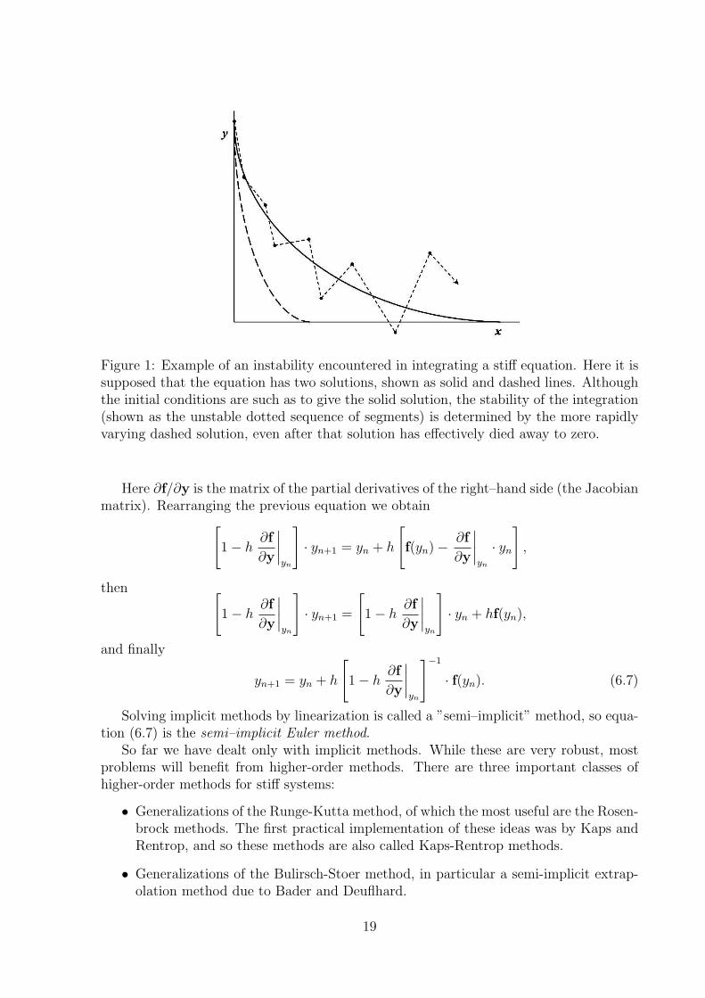
Figure 1: Example of an instability encountered in integrating a stiff equation. Here it issupposed that the equation has two solutions, shown as solid and dashed lines. Althoughthe initial conditions are such as to give the solid solution, the stability of the integration(shown as the unstable dotted sequence of segments) is determined by the more rapidlyvarying dashed solution, even after that solution has effectively died away to zero.

Here ∂f/∂y is the matrix of the partial derivatives of the right–hand side (the Jacobianmatrix). Rearranging the previous equation we obtain

[1− h

∂f

∂y

∣∣∣∣yn

]· yn+1 = yn + h

[f(yn)− ∂f

∂y

∣∣∣∣yn

· yn

],

then [1− h

∂f

∂y

∣∣∣∣yn

]· yn+1 =

[1− h

∂f

∂y

∣∣∣∣yn

]· yn + hf(yn),

and finally

yn+1 = yn + h

[1− h

∂f

∂y

∣∣∣∣yn

]−1

· f(yn). (6.7)

Solving implicit methods by linearization is called a ”semi–implicit” method, so equa-tion (6.7) is the semi–implicit Euler method.

So far we have dealt only with implicit methods. While these are very robust, mostproblems will benefit from higher-order methods. There are three important classes ofhigher-order methods for stiff systems:

• Generalizations of the Runge-Kutta method, of which the most useful are the Rosen-brock methods. The first practical implementation of these ideas was by Kaps andRentrop, and so these methods are also called Kaps-Rentrop methods.

• Generalizations of the Bulirsch-Stoer method, in particular a semi-implicit extrap-olation method due to Bader and Deuflhard.

19

• Predictor-corrector methods, most of which are descendants of Gears backwarddifferentiation method.

6.4 Rosenbrock methods

Now consider the ODE system in the autonomous form

y = f(y), t > t0, y(t0) = y0. (6.8)

This places no restriction since every non-autonomous system can be put in the form(6.8) by treating time t also as a dependent variable.

Rosenbrock methods have the advantage of being relatively simple to understand andimplement. For moderate accuracies and moderate-sized systems, they are competitivewith the more complicated algorithms. For more stringent parameters, theese methodsremain reliable; they merely become less efficient than competitors like the semi-implicitextrapolation method.

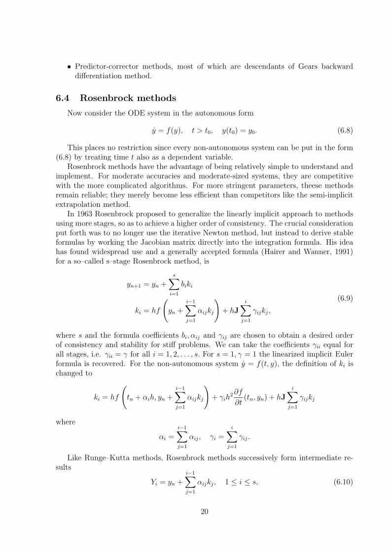
In 1963 Rosenbrock proposed to generalize the linearly implicit approach to methodsusing more stages, so as to achieve a higher order of consistency. The crucial considerationput forth was to no longer use the iterative Newton method, but instead to derive stableformulas by working the Jacobian matrix directly into the integration formula. His ideahas found widespread use and a generally accepted formula (Hairer and Wanner, 1991)for a so–called s–stage Rosenbrock method, is

yn+1 = yn +s∑

i=1

biki

ki = hf

(yn +

i−1∑j=1

αijkj

)+ hJ

i∑j=1

γijkj,

(6.9)

where s and the formula coefficients bi, αij and γij are chosen to obtain a desired orderof consistency and stability for stiff problems. We can take the coefficients γii equal forall stages, i.e. γii = γ for all i = 1, 2, . . . , s. For s = 1, γ = 1 the linearized implicit Eulerformula is recovered. For the non-autonomous system y = f(t, y), the definition of ki ischanged to

ki = hf

(tn + αih, yn +

i−1∑j=1

αijkj

)+ γih

2∂f

∂t(tn, yn) + hJ

i∑j=1

γijkj

where

αi =i−1∑j=1

αij, γi =i∑

j=1

γij.

Like Runge–Kutta methods, Rosenbrock methods successively form intermediate re-sults

Yi = yn +i−1∑j=1

αijkj, 1 ≤ i ≤ s, (6.10)

20

which approximate the solution at the intermediate time points tn + αih. Rosenbrockmethods are therefore also called Runge–Kutta–Rosenbrock methods. Observe that if weidentify J with the zero matrix and omit the ∂f/∂t term, a classical explicit Runge–Kuttamethod results.

Rosenbrock methods are attractive for a number of reasons. Like fully implicit meth-ods, they preserve exact conservation properties due to the use of the analytic Jacobianmatrix. However, they do not require an iteration procedure as for truly implicit methodsand are therefore more easy to implement. They can be developed to possess optimallinear stability properties for stiff problems. They are of one-step type, and thus canrapidly change step size.

For an application of a second order Rosenbrock method applied to photochemicaldispersion problems see [Ver97].

In [Cab] one can found an investigation on a chemical mechanism which demonstratesstiffness. The authors have compared various explicit and implicit numerical methods tosolve the model for the GABA reaction scheme, which is based on the classical bimolecularreaction of Michaelis-Menten, suitably adapted to account for reversible reactions andmultiple receptor states.

In [Vos01] parallel Rosenbrock methods are developed for systems with stiff chemicalreactions.

The authors first have considered the Robertson chemical kinetics problem:

y1 = −0.04y1 + 104y2y3;

y2 = 0.04y1 − 104y2y3 − 3× 107y22;

y3 = 3× 107y22

(6.11)

with initial conditionsy1(0) = 1, y2(0) = 0, y3(0) = 0.

Next they have considered the enzyme kinetics problem of MichaelisMenten type:

∂u

∂t= d

∂2u

∂x2− u

1 + u, d > 0, (x, t) ∈ [0, 1]× [0,∞),

u(x, 0) = 1, u(0, t) = 0, u(1, t) = 0,

(6.12)

whose steady state solution is u = 0.Unlike classical Runge-Kutta methods, parallel Rosenbrock methods avoid the neces-

sity to iterate at each time step. Parallelism across the method allows for the solutionof the linear algebraic systems in essentially backward Euler–like solves on concurrentprocessors. In addition to possessing excellent stability properties, these methods arecomputationally efficient while preserving positivity of the solutions. Numerical resultsapplied to problems above, involving stiff chemistry, and enzyme kinetics confirm thesecharacteristics.

Finally, we mention here that for an application on second order Rosenbrock method

21

one can study the paper of Verwer et al., see [Ver97], where this scheme is defined as:

yn+1 = yn +3

2γk1 +

1

2γk2,

(1

γhI− J

)k1 = f(tn, yn) + γhft,

(1

γhI− J

)k2 = f(tn + h, yn +

1

γk1)− 2

γhk1 − γhft,

(6.13)

with γ = 1 + 1/√

2. In [Ver97] it was noted that the second order Rosenbrock methodhave favorable positivity properties, and the method is stable for nonlinear problems evenwith large fixed step sizes.

6.5 Semi-implicit extrapolation method

The Bulirsch–Stoer method, which discretizes the differential equation using the mod-ified midpoint rule, does not work for stiff problems. Bader and Deuflhard discovereda semi–implicit discretization that works very well and that lends itself to extrapolationexactly as in the original Bulirsch–Stoer method. The starting point is an implicit formof the midpoint rule:

yn+1 − yn−1 = 2hf

(yn+1 + yn−1

2

)(6.14)

Convert this equation into semi-implicit form by linearizing the right-hand side aboutf(yn). The result is the semi–implicit midpoint rule:

[1− h

∂f

∂y

]· yn+1 =

[1 + h

∂f

∂y

]· yn−1 + 2h

[f(yn)− ∂f

∂y· yn

]. (6.15)

It is used with a special first step, the semi-implicit Euler step (6.7), and a special”smoothing” last step in which the last yn is replaced by

yn :=1

2(yn+1 + yn−1). (6.16)

Bader and Deuflhard showed that the error series for this method once again involvesonly even powers of h.

For practical implementation, it is better to rewrite the equations using ∆k = yk+1−yk.With h = H/m, start by calculating

∆0 =

[1− h

∂f

∂y

]−1

· hf(y0)

y1 = y0 + ∆0.

(6.17)

Then for k = 1, 2, . . . , m− 1, set

∆k = ∆k−1 + 2

[1− h

∂f

∂y

]−1

· [hf(yk)−∆k−1],

yk+1 = yk + ∆k.

(6.18)

22

Finally compute

∆m =

[1− h

∂f

∂y

]−1

· [hf(ym)−∆m−1],

ym = ym + ∆m.

(6.19)

6.6 Gear algorithm

Consider the ODE system

y = f(y, t), t > t0, y(t0) = y0. (6.20)

arising from chemistry.In what follows we will present here the Gear algorithm in reference to the above

system.The Gear algorithm is one of a class of methods referred to as backward differentiation

formulae (BDF). The generalized BDF that forms the basis for Gear’s method can beexpressed as follows:

yn = hβ0f(yn, tn) +

p∑j=1

αjyn−j (6.21)

where n refers to the time step, h is the size of the time step, p is the assumed order,β0 and αj are scalar quantities that are functions of the order, and f(y, t) is the functionwhich describe the rate of change of each species concentration in a chemical mechanism.The method is implicit since concentrations at the desired time step n depend on valuesof the first derivatives contained in f(yn, tn) that are functions of the concentrations atthe same time. The order of the method corresponds to the number of concentrationsat previous time steps that are incorporated in the summation on the right hand side ofequation (6.21).

To facilitate changing step size and estimating errors, the multi-step method in equa-tion (6.21) is transformed to a multi-value form in which information from only the pre-vious step is retained, but information on higher order derivatives is now used. In thisformulation, the solution is first approximated by predicting concentrations and higherorder derivatives at the end of a time step for each species using the following matrixequation:

zi,n,(0) = Bzi,n−1 (6.22)

where zi = [yi, hy′i, . . . , hpyiy(p)i /p!]>, the subscript n, (0) refers to the prediction at the

end of time step n, and the subscript n−1 refers to values obtained at the end of previoustime step (or the initial conditions when n = 1). B is the Pascal triangle matrix, thecolumns of which contain the binomial coefficients.

The prediction obtained from equation (6.22) is then corrected by solving for zi,n suchthat the following relations hold for all species:

zi,n = zi,n,(0) + r[hfi(yn, tn)− hy′i,n,(0)]. (6.23)

In equation (6.23), r is a vector of coefficients that is dependent on the order, butr2, the element corresponding to the first derivative location in z, is always equal to one.

23

Thus, the correct value of yi,n is obtained when the calculated value of y′i,n equals fi(yn, tn)in equation (6.23). An approximate solution for yi,n is obtained by applying Newton’smethod to the system of equations that correspond to the first equation in (6.23) for allspecies. This leads to the following corrector iteration equation:

yn,(m+1) = yn,(m) + [I− hβ0J]−1r1[hf(yn,(m), tn)− hδyn,(m)] (6.24)

where m refers to the Newton iteration number, the vector f(yn, tn) is calculated usingconcentrations computed for the mth iteration, δc is the vector containing the most recentestimates of first derivatives, I is the identity matrix, and J is the Jacobian matrix whoseentries are defined as:

Jij =∂fi(y, tn)

∂yj

; i, j = 1, 2, . . . , N. (6.25)

At the end of each iteration, the vector containing the first derivatives (δc) is updated,but higher order derivatives in z need not be computed until convergence is achieved.

Although several variants of the basic Gear algorithm have been developed, the fun-damental computational scheme can be described generically as follows. At the beginningof any integration interval, the order is set to one and the starting time step is eithercalculated or selected by the user. Each time step is initiated by predicting concentra-tions at the end of the time step using equation (6.22). Corrector iterations are thencarried out using equation (6.24) until prescribed convergence criteria are achieved ornon-convergence is deemed to have occurred.

We have to mention here that Jacobson and Turco (1994) have modified the Gearalgorithm to incorporate additional computational efficiencies that can achieve speedupson the order of 100 on vector computers. About half of the improvement is attributed toenhanced vectorization, and half to improved matrix operations.

6.7 Multistep, multivalue, and predictor-corrector methods

The terms multistep and multivalue describe two different ways of implementing es-sentially the same integration technique for ODEs. Predictor–corrector is a particularsubcategory of these methods in fact, the most widely used. Accordingly, the namepredictor–corrector is often loosely used to denote all these methods.

To advance the solution of y′ = f(x, y) from xn to x, we have

y(x) = yn +

∫ x

xn

f(x′, y)dx′. (6.26)

In a multistep method, we approximate f(x, y) by a polynomial passing through severalprevious points xn, xn−1, . . . and possibly also through xn+1. The result of evaluating theintegral (6.26) at x = xn+1 is then of the form

yn+1 = yn + h(β0y′n+1 + β1y

′n + β2y

′n−1 + β3y

′n−2 + . . .) (6.27)

where y′n denotes f(xn, yn), and so on. If β0 = 0, the method is explicit; otherwise it isimplicit. The order of the method depends on how many previous steps we use to geteach new value of y.

24

Consider how we might solve an implicit formula of the form (6.27) for yn+1. Twomethods suggest themselves: functional iteration and Newtons method. In functionaliteration, we take some initial guess for yn+1, insert it into the right-hand side of (6.27)to get an updated value of yn+1, insert this updated value back into the right-hand side,and continue iterating. To get an initial guess for yn+1 one must use some explicit for-mula of the same form as (6.27) This is called the predictor step. In the predictor stepwe are essentially extrapolating the polynomial fit to the derivative from the previouspoints to the new point xn+1 and then doing the integral (6.26) from xn to xn+1. Thesubsequent Simpson-like integration, using the prediction steps value of yn+1 to interpo-late the derivative, is called the corrector step. The difference between the predicted andcorrected function values supplies information on the local truncation error that can beused to control accuracy and to adjust step size.

The most popular predictor-corrector methods are probably the Adams- Bashforth-Moulton schemes, which have good stability properties. The Adams- Bashforth part isthe predictor.

The Adams-Bashforth formula has the form

xi+1 = xi +n∑

j=1

cjfj, where fj = f(ti−(j−1), x(ti−(j−1))).

Note the formula uses the function values at points left to ti, namely, at ti, ti−1, . . . , ti−(n−1).To determine the coefficients in the Adams-Bashforth formula one have to solve a

linear system for the cj’s,

∫ 1

0

r(i−1)dr =n∑

j=1

(cj(1− j)(i−1)

)

where 1, r, r2, . . . , r(n−1) are the testing polynomials.For example the the 2nd-order Adams-Bashforth method becomes as follow:

x0 = x0, x1 = x1, xi+1 = xi +h(3f(ti, xi)− f(ti−1, xi−1))

2

for i > 0.In practice, Adams-Bashforth formula is not used alone. Neither does Adams-Moulton

formula. Instead, the Adams-Moulton formula, which is implicit, is modified by approx-imating xi+1 using the solution we get from the Adams-Bashforth method. This avoidssolving a nonlinear equation for xi+1 in the original Adams-Moulton formula, and improvesaccuracy of the Adams-Bashforth formula.

For instance, the 2nd-order Adams-Bashforth formula and the 2nd-order Adams-Moulton formula lead us to a second order predictor–corrector method:

x0 = x0, x1 = x1,

yi+1 = xi +h(3f(ti, xi)− f(ti−1, xi−1))

2,

xi+1 = xi +h(f(ti+1, yi+1) + f(ti, xi))

2.

(6.28)

25

7 Positive and conservative numerical methods

There exist specialized softwares that translate kinetic reactions into differential equa-tions (e.g., KPP [Dam02]). As we mentioned earlier, the ODEs describing chemical ki-netics can be nonlinear and very stiff. The stiffness in these systems forces the use ofimplicit numerical techniques for their solution. The drawback to the use of an implicitnumerical technique is the need to solve a large nonlinear algebraic system of equations foreach numerical time step at each spatial grid point. The greater the number of chemicalspecies modeled, the larger the resulting system. Thus, the numerical overhead associatedwith solving these nonlinear algebraic systems can account for a significant portion of thetotal runtime, for example, in atmospheric sciences (reactive flow problem, combustion,climate modeling, chemical-radiative-transport model).

Several recent studies have proposed techniques that effectively eliminate the need forthe matrix algebra typically associated with an implicit numerical method, for instance,the preconditioned implicit methods. That study led to the development of the ChemicalSolver for Ordinary Differential Equations (CHEMSODE) package to support the use ofthese methods. The paradigm of the preconditioned implicit methods combine an implicitODE integration formula with an iterative technique for solving simultaneous algebraicsystems. This idea is illustrated in [Aro96] and have been drawn from two previous stud-ies. The above report documents the CHEMSODE package: a collection of FORTRANsubroutines implementing three different types of preconditioned time differencing tech-niques along with a choice of step length control.

A comparison between two classical integrators for stiff ordinary differential equations,Quasi Steady State Approximation (QSSA), and Hybrid Solver (HS), and CHEMSODEpackage is presented in [Lor99]. The results have been compared with an ”exact” solutionobtained by the Livermore Solver for Ordinary Differential Equations (LSODE).

A comprehensive numerical comparison between some(other) explicit and implicitsolvers can also be found in [San97]. For another comparison of numerical methods forthe integration of kinetic equations in atmospheric chemistry and transport models, see[Say95].

When fast reversible reactions precede slower ones in a mechanism, in order to deriveapproximate analytical expressions, beside the QSSA classical method we can use anotheruseful approximation method, the pre-equilibrium approximation (PEA), also called equi-librium approximation. Both approximations can also be used to simplify the numericalintegration of complex reaction schemes, reducing the dimensionality and decoupling timescales. In their work, see [Rae02], M. Rae and N. Berberan–Santos were presented a gen-eral view of the pre-equilibrium approximation via several photophysical systems. Theyalso have shown that the kinetic behavior of systems subject to pre-equilibration can beobtained by the application of perturbation theory.

Air quality models solve the convection-diffusion reaction set of partial differentialequations which describe the atmospheric physical and chemical processes. Usually anoperator-split approach is taken: chemical equations and convectiondiffusion equations aresolved in alternative steps. In this setting the integration of chemical kinetic equations isa demanding computational task. The chemical integration algorithm should be stable inthe presence of stiffness; ensure a modest level of accuracy, typically 1%; preserve mass;and keep the concentrations positive. Since chemical kinetics conserves mass and renders

26

nonnegative solutions a good numerical simulation would ideally produce mass-balanced,positive concentration vectors. Many time-stepping methods are mass conservative (mul-tistep, Runge-Kutta, Rosenbrock); however, unconditional positivity restricts the orderof a traditional method to one. Clipping (setting the negative concentrations to zero)enhances stability but artificially adds mass to the system. In [San97] was presented aprojection method which ensure mass conservation and positivity, alleviating the orderand step-size restrictions. The solutions computed at each step by a standard integrationmethod are ”projected” back onto the reaction simplex. The resulting vectors betterapproximate the true solution itself.

Another approach to accelerate reacting flow calculations was proposed by O. Knothand R. Wolke in [Kno98]. The authors gave implicit-explicit time integration schemeswhich use explicit higher order Runge-Kutta schemes for the integration of the horizontaladvection. The stiff chemistry and all vertical transport processes (turbulent diffusion,advection, deposition) are integrated in an implicit and coupled manner by a higher orderbackward differentiation formula method.

7.1 Stiff systems related to mass action kinetics

Numerical schemes that maintain numerical analogous of physical properties such asnonnegativity of the solution and atomic mass conservation without time step restrictionsare also described in [Ber96]. Classical explicit schemes maintain these properties withtoo strong time-step restrictions to be useful. Classical implicit schemes maintain theseproperties with weaker time-step restrictions, but require the solution of an algebraicsystem at each time step. In the above mentioned paper, E. Bertolazzi proposed anddiscussed the solution of these algebraic systems without the use of Jacobian matrices, butby the repeated inversion of M-matrices that can be easily constructed, thus considerablysimplifying and accelerating the computer implementation of the schemes.

To illustrate the idea consider a reaction mechanismm∑

i=1

α(i, r)Xi ­m∑

i=1

β(i, r)Xi r = 1, 2, . . . , k

which can be written in the formm∑

i=1

σ(i, r)Xi = 0, r = 1, 2, . . . , k. (7.1)

The associated system of polynomial differential equation describing the time evolutionof the species concentrations can be written as

dx

dt= σw(x), (7.2)

where x =

x1

x2...

xm

, σ =

σ(1, 1) σ(1, 2) . . . σ(1, k)σ(2, 1) σ(2, 2) . . . σ(2, k)

...... . . .

...σ(m, 1) σ(m, 2) . . . σ(m, k)

, w(x) =

w1(x)w2(x)

...wk(x)

are the

molar concentration vector, the stoichiometric matrix and the reaction velocity vector,respectively.

27

If Mi is the atomic mass of the ith species, then ρi = Mixi is its density. Defining

D = diag(M1,M2, . . .Mm),

ρ = Dx,

f(ρ) = w(D−1ρ),

ν = Dσ,

chemical system (7.1) can be written in term of densities as follows:

dρ

dt= νf(ρ). (7.3)

We have to mention here that in mass action kinetic reaction rates often have the formf(ρ) = cρα1

1 ρα22 . . . ραm

m , where c is a constant and αi ≥ 0.Related to equation (7.3), it is important that, there exist two general requirements

(see [Ber96]):

• one for the reaction rate f with its stoichiometric vector ν

(i) f ∈ C(Rm

+ ,R+),

(ii) if νi < 0, then the function q(ρ) := f(ρ)/ρi is such that q ∈ C(Rm

+ ,R+)

• the other is connected with the nonnegativity of the solution:

if ρ0 ≥ 0 =⇒ ∀t > 0, ρ(t; ρ0) ≥ 0 (7.4)

where ρ(t; ρ0) denotes the solution of system (7.3) with ρ0 as initial value.Now, consider the kernel ν>, i.e., Ker(ν>) = {z|zν> = 0}. If z ∈ Ker(ν>) then from

(7.3), it follows that z>dρ

dt= z>νf(ρ) = 0, so that the function

gz(ρ) = z>ρ = z1ρ1 + · · ·+ zmρm, z ∈ Ker(ν>) (7.5)

is a first integral of (7.3). In the case of a conservative system, we have ||ρ||1 = ρ1 +ρ2 + · · ·+ ρm = constant so that ge is a first integral of the system (7.3), or equivalently,e ∈ Ker(νT ), where e = [1, 1, . . . , 1]>.

In what follows we will take a survey through some classical numerical schemes toestablish whether mass conservation and positivity preservation is realized.

A general numerical one-step scheme can be written as

ρn+1 = G(ρn), n = 1, 2, . . . (7.6)

For this scheme the conservation and nonnegativity properties (7.5) can be written as

G(ρ) ≥ 0, ∀ρ ≥ 0, (7.7a)

z>(ρ−G(ρ)) = 0, ∀z ∈ Ker(ν>), ∀ρ ≥ 0. (7.7b)

We will consider a single reaction system

dρ

dt= νf(ρ), (7.8)

where the reaction rate f is an homogeneous function of degree 1, for example f(ρ) =

cρα11 ρα2

2 . . . ραmm , with αi =

{1, if νi < 0,0, if νi ≥ 0,

and discretize (7.8) with some classical schemes.

28

7.1.1 Explicit Euler scheme

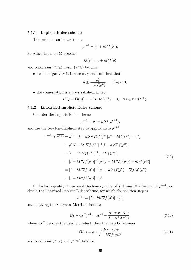
This scheme can be written as

ρn+1 = ρn + hνf(ρn),

for which the map G becomes

G(ρ) = ρ + hνf(ρ)

and conditions (7.7a), resp. (7.7b) become

• for nonnegativity it is necessary and sufficient that

h ≤ ρni

−νif(ρn), if νi < 0,

• the conservation is always satisfied, in fact

z>(ρ−G(ρ)) = −hz>νf(ρn) = 0, ∀z ∈ Ker(ν>).

7.1.2 Linearized implicit Euler scheme

Consider the implicit Euler scheme

ρn+1 = ρn + hνf(ρn+1),

and use the Newton–Raphson step to approximate ρn+1

ρn+1 ≈ ρn+1 = ρn − [I − hν∇f(ρn)]−1[ρn − hνf(ρn)− ρn]

= ρn[I − hν∇f(ρn)]−1[I − hν∇f(ρn)]−

− [I − hν∇f(ρn)]−1[−hνf(ρn)]

= [I − hν∇f(ρn)]−1[ρn(I − hν∇f(ρn)) + hνf(ρn)]

= [I − hν∇f(ρn)]−1[ρn + hν (f(ρn)−∇f(ρn)ρn)]

= [I − hν∇f(ρn)]−1ρn.

(7.9)

In the last equality it was used the homogeneity of f. Using ρn+1 instead of ρn+1, weobtain the linearized implicit Euler scheme, for which the solution step is

ρn+1 = [I − hν∇f(ρn)]−1ρn,

and applying the Sherman–Morrison formula

(A + uv>)−1 = A−1 − A−1uv>A−1

I + v>A−1u, (7.10)

where uv> denotes the dyadic product, then the map G becomes

G(ρ) = ρ +hν∇f(ρ)ρ

I − h∇f(ρ)ν (7.11)

and conditions (7.7a) and (7.7b) become

29

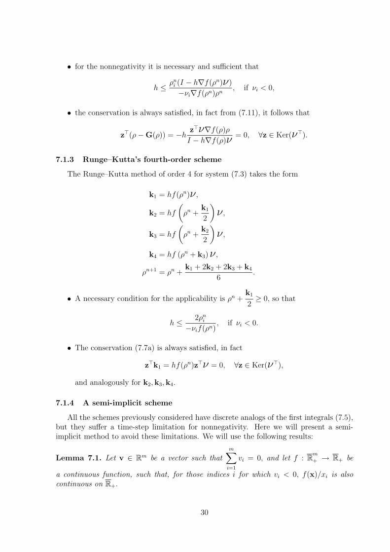
• for the nonnegativity it is necessary and sufficient that

h ≤ ρni (I − h∇f(ρn)ν)

−νi∇f(ρn)ρn, if νi < 0,

• the conservation is always satisfied, in fact from (7.11), it follows that

z>(ρ−G(ρ)) = −hz>ν∇f(ρ)ρ

I − h∇f(ρ)ν = 0, ∀z ∈ Ker(ν>).

7.1.3 Runge–Kutta’s fourth-order scheme

The Runge–Kutta method of order 4 for system (7.3) takes the form

k1 = hf(ρn)ν ,

k2 = hf

(ρn +

k1

2

)ν ,

k3 = hf

(ρn +

k2

2

)ν ,

k4 = hf (ρn + k3)ν ,

ρn+1 = ρn +k1 + 2k2 + 2k3 + k4

6.

• A necessary condition for the applicability is ρn +k1

2≥ 0, so that

h ≤ 2ρni

−νif(ρn), if νi < 0.

• The conservation (7.7a) is always satisfied, in fact

z>k1 = hf(ρn)z>ν = 0, ∀z ∈ Ker(ν>),

and analogously for k2,k3,k4.

7.1.4 A semi-implicit scheme

All the schemes previously considered have discrete analogs of the first integrals (7.5),but they suffer a time-step limitation for nonnegativity. Here we will present a semi-implicit method to avoid these limitations. We will use the following results:

Lemma 7.1. Let v ∈ Rm be a vector such thatm∑

i=1

vi = 0, and let f : Rm

+ → R+ be

a continuous function, such that, for those indices i for which vi < 0, f(x)/xi is alsocontinuous on R+.

30

Then f(x)v can be written as

C(x,v)x = f(x)v,

where C(x,v) is m×m matrix with continuous entries such that

Ci,i(x,v) ≤ 0, i = 1, 2, . . . ,m,

Ci,j(x,v) ≥ 0, i 6= j,m∑

i=1

Ci,j(x,v) = 0, i = 1, 2, . . . , m.

(7.12)

Theorem 7.1. Let ν be a m× k matrix and f : Rm

+ → Rk

+ be a continuous map; then iffor those indices i, j for which νi,j < 0,

fi(x)

xj

,

is also continuous on Rn

+, and

m∑i=1

vi,j = 0, j = 1, 2, . . . , k,

then νf(ρ) can be written in the form C(ρ,ν)ρ, where C(ρ,ν) is a m ×m matrix withcontinuous entries, such that

i) Ci,i(ρ,ν) ≤ 0, i = 1, 2, . . . , m,

ii) Ci,j(ρ,ν) ≥ 0, i 6= j,

iii)m∑

i=1

Ci,j(ρ,ν) = 0, i = 1, 2, . . . , m.

For the proof of the lemma and the theorem above, the definition of matrix C(x,v)see [Ber96].

With the matrix C, it is possible to define a semi-implicit numerical scheme for (7.3)as follows:

ρn+1 = ρn + hC(ρn,ν)ρn+1,

which results in the following advancing step:

ρn+1 = [I − hC(ρn,ν)]−1ρn.

The matrix I − hC(ρn,ν) is strictly diagonally dominant with elements positive onthe diagonal and nonnegative elsewhere, consequently, it is a M -matrix. By definition oda M -matrix, it follows that I − hC(ρn,ν)−1 ≥ 0, and therefore, ρn+1 ≥ 0 for arbitrarilylarge h. Unfortunately, this scheme has not a numerical analogs of first integral (7.5).

31

7.1.5 A fully implicit scheme

All the previous considered schemes cannot have both a discrete analogs of first integral(7.5) and nonnegativity preservation for arbitrarily large time step. The implicit Eulerscheme

ρn+1 = ρn + hνf(ρn+1) (7.13)

can be used to avoid time-step restrictions, but the advancing steps involve the solutionof a nonlinear system as follows:

ρn+1 = the solution of x− hνf(x)− ρn = 0. (7.14)

For system (7.14), there is the question of existence and uniqueness of the solution andan iterative procedure is needed to find the solution.

Existence of a solution: A nonnegative solution of the nonlinear system

x− hνf(x)− ρn = 0, (7.15)

is also, by Theorem 7.1, a fixed point of the map

Φ(x) := (I − hC(x,ν))−1ρn. (7.16)

Theorem 7.2. The map Φ admits at least one nonnegative fixed point (i.e., with non-negative components). Moreover if x∗ is a nonnegative fixed point, then ||x∗||1 = ||ρn||1.Proof. The map Φ has the property ∀ρ ≥ 0 =⇒ Φ(ρ) ≥ 0, and from (7.16), we can write

Φ(x)− hC(x,ν)Φ(x) = ρn, (7.17)

multiplying (7.17) by e> and using the fact e>C(x,ν), it follows

e>Φ(x) = e>ρn =⇒ ||Φ(x)||1 = ||ρn||1, ∀x ≥ 0.

Consequently, the image Φ(Rn

+) is contained into the convex compact

K = {x ≥ 0|||x||1 = ||ρn||1}, (7.18)

so that, if x∗ is a fixed point, it must be contained in K and ||x||1 = ||ρn||1. Moreover,the map Φ can be viewed as a continuous map from K into K, and by the Brouwer fixedpoint theorem it follows that Φ has at least one fixed point.

Observe that the proof is independent of the magnitude of h, so that the nonlinearsystem (7.15) has a nonnegative solution no matter how large the time step is.

32

The question of uniqueness: In general, it is not possible to see if system (7.15) hasa unique solution for arbitrarily large h. However, there are some special cases for whichwe have also uniqueness. It is the case, for instance, when the system consists of only onereaction and the reaction rate f satisfies

νi∂fρi ≤ 0, i = 1, 2, . . . ,m,

which exclude auto-inhibition in the reaction. In this case, if x∗ and y∗ are two solutionsof (7.15), it follows

0 = x∗ − y∗ − hν [f(x∗)− f(y∗)] = [I − hν∇f(ξ)](x∗ − y∗), (7.19)

and using the Sherman-Morrison formula (7.10)

[I − hν∇f(ξ)]−1 = I +hν∇f(ξ)

I − hν∇f(ξ), (7.20)

so that by (7.19) and (7.20), it follows that x∗ = y∗. In the case of more than one reaction,it is possible to prove uniqueness for small h.

Theorem 7.3. Let νf(ρ) be a m × k matrix and f ∈ C1(Rm+,R+), then if for those

indices i, j for which νi,j < 0,

fi(x)

xj

∈ C1(Rm+,R+),

then for all h satisfying

h <1

m||ρn||1 maxz∈K ||∇Ci,j(z,ν)||∞ ,

the map Φ : Rm

+ → Rm

+ defined in (7.16) is a contraction, where K is given by (7.18).

Proof. Observe that ∀z ≥ 0

e>[I − hC(z,ν)] = e> =⇒ e> = e>[I − hC(z,ν)]−1,

so that it follows ||[I − hC(z,ν)]−1||1 = 1. Next

Φ(x)− Φ(y) = [I − hC(x,ν)]−1ρn − [I − hC(y,ν)]−1ρn =

= h[I − hC(x,ν)]−1[C(x,ν)−C(y,ν)][I − hC(y,ν)]−1ρn,

and taking the || · ||1 norm on both sides

||Φ(x)− Φ(y)||1 ≤ h||C(x,ν)−C(y,ν)||1||ρ||1 ≤ hL||x− y||1,where

L = m||ρn||1 maxz∈K

||∇ci,j(z,ν)||∞,

so that if h <1

Lthe map Φ becomes a contraction.

Obviously, if the map Φ is a contraction, then it has a unique fixed point.

33

7.1.6 A second-order positive scheme

The implicit Euler scheme has no stability restriction, but it is only first-order accurate.A second-order scheme can be the following:

ρn+1 = ρn + hν f(ρn+1) + f(ρn)

2.

The solution step, as in (7.13), involves the solution of a nonlinear system in the unknownx

x− hf(x)

2= ρn + h

νf(ρn)

2.

In order to guarantee the existence of a nonnegative solution, it is sufficient that:

ρn + hνf(ρn)

2≥ 0.

This condition introduces a time-step bound. To avoid time-step restriction, an alternativeapproach is to switch to second-order accuracy when reactions are slow and first-orderaccuracy when reactions are fast. The scheme becomes

ρn+1 = ρn + hν [(1− α)f(ρn+1) + αf(ρn], (7.21)

where α is such thatmax

α∈[0,1/2][ρn + αhνf(ρn)] ≥ 0.

If the reaction rates have very different orders of magnitudes, this scheme can loose toomuch accuracy for slow reactions. a better result can be obtained y using different α’s foreach reaction as follows:

ρn+1 = ρn + h

k∑j=1

ν·,j[(1− αi)fj(ρn+1) + αjfj(ρ

n)]. (7.22)

With (7.22), the solutio step involves the solution of the nonlinear system in the unknownx

x− h

k∑j=1

(1− αj)ν·,jfj(x) = ρn + h

k∑j=1

αjν·,jfj(ρn).

For positivity preservation, it suffices that

ρn +k∑

j=1

αjν·,jfj(ρn) ≥ 0. (7.23)

In order to satisfy condition (7.23), we set

αj = min

(1

2,

{− βjρ

ni

hνi,jfj(ρn)|νi,j < 0, i = 1, 2, . . . , m

}),

where βj > 0 are weighting parameters with∑k

j=1 βj = 1. The weighting factors are useful;if, for example, the first reaction is very slow, we can use very small β1 and maintainα1 = 1/2. This permits us to increase the α’s for the fast reactions. The weighting factorscan be chosen in many ways. A simple choice could be βi = 1/k.

34

7.1.7 Two better second-order positive schemes

The scheme (7.21) has the disadvantage of slowing down the accuracy for time stepsthat are large compared to the reaction rates. An alternative can be an implicit versionof Collatz scheme which takes the form

ρn+1 = ρn + hνf

(ρn+1 − h

2νf(ρn+1)

). (7.24)

Equation (7.24) involves the solution of the nonlinear system in the unknown x

x− hνf

(x− h

2νf(x)

)= ρn. (7.25)

To solve (7.25), we will introduce a new variable

y = x− h

2νf(x),

so that system (7.25) is equivalent to the new system

x− hνf(y) = ρn, x− h

2νf(x) = y. (7.26)

This system, by Theorem 7.1, can be written in the following equivalent form:

λy − hC(y,ν)y = ρn − x + λy, x− h

2C(x,ν)x = y,

where λ is a free parameter. This relation suggests the following iterative procedure tosolve (7.26)

yl+1 =

(I − h

λC(yl,ν)

)−1 (ρn − xl

λ+ yl

),

xl+1 =

(I − h

2C(xl,ν)

)−1

yl+1.

(7.27)

Another scheme can be an implicit version of Heun scheme which takes the form

ρn+1 = ρn + h1

2ν [f(ρn+1 − hνf(ρn+1)) + f(ρn+1)]. (7.28)

Equation (7.28) involves the solution of the nonlinear system in the unknown x

x− h

2ν [f(x− hνf(x)) + f(x)] = ρn. (7.29)

To solve (7.29), it is convenient to introduce a new variable

y = x− hνf(x),

so that the system is equivalent to the new system

y − hνf(y) = 2ρn − x, x− hνf(x) = y.

35

The equivalent form of this system applying Theorem 7.1 will be

(1 + λ)y − hC(y,ν)y = 2ρn − x + λy, x− hC(x,ν)x = y.

This suggests the following iterative procedure to solve (7.26)

yl+1 =((1 + λ)I − hC(yl,ν)

)−1(2ρn − xl + λyl),

xl+1 =(I − hC(xl,ν)

)−1yl+1.

(7.30)

7.1.8 A second-order diagonally implicit Runge–Kutta scheme

The schemes (7.24) and (7.28) have the disadvantage of a slow rate of convergenceof the procedures (7.27) and (7.30). An alternative can be the use of diagonally implicitRunge–Kutta schemes, so that, instead of solving a large nonlinear system, we solve aseries of smaller nonlinear systems. For example the S-stable two-stage diagonally implicitRunge–Kutta scheme of Alexander after some manipulation takes the form

x− αhνf(x) = ρn,

y − αhνf(x) =(2α− 1)ρn + (1− α)x

α,

ρn+1 = y,

(7.31)

where α = 1±√2/2.

8 Solving stiff IVP’s with Maple

Maple is a procedural programming language. It is a computer algebra software thatcan perform symbolic computation as well as numerical computation, graphics, program-ming, and more. It can handle differential equations, too. Sometimes Maple can solvethem symbolically, finding the general solution. If the equation can not be solved sym-bolically, one can always find a numerical answer.

If it takes too long to solve an initial value problem (IVP) with the default numeri-cal solver (for example, rkf45, which stands for Fehlberg fourth-fifth order Runge-Kuttamethod) then the IVP might be stiff. A stiff IVP can be solved efficiently with either thedefault solver using the stiff=true option (rosenbrock) in dsolve command or any of theback- options in lsode. Obtained numerical solutions may be plotted using the odeplotcommand in the plots package.

First we initialize Maple.> restart;with(DEtools):with(plots):with(linalg):

The equation we wish to solve a second order ODE y′′(x)+ (λ+1)y′(x)+λ y = 0 withthe initial conditions y(0) = 1, y’(0)=-1.

36

By introducing auxiliary variables we can convert it into a set of first order ODEs,where λ is a constant:

y′(x) = z(x)

z′(x) = −λ y(x)− (λ + 1)z(x).

We shall investigate how varying λ affects the numerical solution. The above is anexample of a stiff equation. If we solve the above analytically, we find that: y(x) = e−x.We also have an unwanted solution where y(x) = e−λ x.

We will show that under certain circumstances forward Euler fails to converge to thereal solution, and instead blows up to infinity. In fact forward Euler is only stable for thestep sizes that satisfy h < 2λ−1.

Now we will present two implementations of forward and backward Euler to modelthe stiff equation:

> GeneralForwardEuler := proc(vars, f, init, h, interval)local makeeqn, ans, solveEqns, assignList, diffValue, newICSet,i,j,k, ic; ic := init;makeeqn := nops(u);ans := [];ans := [op(ans), ic];

while op(1,ic) < interval dosolveEqns := [];assignList := [];for j from 1 by 1 to makeeqn doassignList := [op(assignList), op(j, u) = op(j, ic)];end do;for i from 1 by 1 to makeeqn dodiffValue := eval(op(i, f),assignList);solveEqns := [op(solveEqns),op(i, u) = op(i, ic) + h * (diffValue)];end do;newICSet := solve(convert(solveEqns, set), convert(u, set));for k from 1 by 1 to makeeqn doic := subsop(k = eval(op(k, u), newICSet), ic);end do;ans := [op(ans), ic];end do;

return matrix(ans);end proc:> GeneralBackwardEuler := proc(vars, f, init, h, interval)local makeeqn, ans, solveEqns, assignList, diffValue, newICSet, i, j, k,ic;ic := init;makeeqn := nops(u);ans := [];ans := [op(ans), ic];

while op(1,ic) < interval dosolveEqns := [];assignList := [];for j from 1 by 1 to makeeqn do

37

assignList := [op(assignList), op(j, u) = op(j, ic)];end do;for i from 1 by 1 to makeeqn dodiffValue := eval(op(i, f), assignList);solveEqns := [op(solveEqns), op(i, u) = op(i, ic) + h * (op(i, f))];end do;newICSet := solve(convert(solveEqns, set),convert(u, set));for k from 1 by 1 to makeeqn doic := subsop(k = eval(op(k, u), newICSet), ic);end do;ans := [op(ans), ic];end do;

return matrix(ans);end proc:

To investigate how varying the value of λ changes the nature of the numericalsolution, first take λ = 1000 and h = 0.1.> u := [x,y,z];f := [1,z,-la103*y - (la103 + 1)*z];ic := [0,1,-1];

u := [x, y, z]

f := [1, z,−1000 y − 1001 z]

ic := [0, 1,−1]

> la103 := 10^3;la103 := 1000

If we limit the range for x = [0, 1.5], there doesn’t seem to be a problem, until x = 1.5where we have a sudden jump in value.

> solBE1 := GeneralBackwardEuler(u,f,ic,0.1,1.5):solFE1 := GeneralForwardEuler(u,f,ic,0.1,1.5):plot_yz := []:plot_yzLa := []:plot_yz1 := []:plot_yz2 := []:

for i from 1 by 1 to 16 doplot_yz := [op(plot_yz),[solBE1[i,1], exp(-solBE1 [i,1])]]:plot_yzLa := [op(plot_yzLa),[solBE1[i,1], exp(-la103*(solBE1 [i,1]))]]:plot_yz1 := [op(plot_yz1),[solBE1[i,1], solBE1[i,2]]]:plot_yz2 := [op(plot_yz2),[solFE1[i,1],solFE1[i,2]]]:end do:

plotsetup("ps", plotoptions="color");plot([plot_yz, plot_yzLa, plot_yz1, plot_yz2], legend=["Real sol", "Unwantedsol", "Backward Euler","Forward Euler"], colour=[green, brown, red, black],style=[line,line,line, point]);plotsetup(default);plot([plot_yz, plot_yzLa, plot_yz1, plot_yz2], legend=["Real sol", "Unwantedsol", "Backward Euler","Forward Euler"], colour=[green, brown, red, black],style=[line,line,line, point]);

38

1

0.6

0.8

0.4

0.4

0

0.2

1.41.210.80.20 0.6

Real sol

Unwanted sol

Backward Euler

Forward Euler

However, when increasing the range to x = 1.6, we find that forward Euler breaks downfar more significantly. Increasing x further, and forward Euler becomes very unstable,blowing up to infinity.

> solBE2 := GeneralBackwardEuler(u,f,ic,0.1,1.6):solFE2 := GeneralForwardEuler(u,f,ic,0.1,1.6):plot_yz := []:plot_yzLa := []:plot_yz1 := []:plot_yz2 := []:

for i from 1 by 1 to 17 doplot_yz := [op(plot_yz),[solBE2[i,1], exp(-solBE2 [i,1])]]:plot_yzLa := [op(plot_yzLa),[solBE2[i,1], exp(-la*(solBE2 [i,1]))]]:plot_yz1 := [op(plot_yz1),[solBE2[i,1], solBE2[i,2]]]:plot_yz2 := [op(plot_yz2),[solFE2[i,1],solFE2[i,2]]]:end do:

39

plotsetup("ps", plotoptions="color");plot([plot_yz, plot_yzLa, plot_yz1, plot_yz2], legend=["Real sol", "Unwantedsol", "Backward Euler","Forward Euler"], colour=[green, brown, red, black],style=[line,line,line, point]);plotsetup(default);plot([plot_yz, plot_yzLa, plot_yz1, plot_yz2], legend=["Real sol", "Unwantedsol", "Backward Euler","Forward Euler"], colour=[green, brown, red, black],style=[line,line,line, point]);

0.80

-40

0.40

-60

-80

1.61.2

-20

Real sol

Unwanted sol

Backward Euler

Forward Euler

Now we can try h=0.01. Here we find that forward Euler breaks down far quicker, inspite of having a step size.

> solBE3 := GeneralBackwardEuler(u,f,ic,0.01,0.2):sol6 := GeneralForwardEuler(u,f,ic,0.01,0.2):plot_yz := []:plot_yzLa := []:plot_yz1 := []:plot_yz2 := []:

for i from 1 by 1 to 21 do

40

plot_yz := [op(plot_yz),[solBE3[i,1], exp(-solBE3 [i,1])]]:plot_yzLa := [op(plot_yzLa),[solBE3[i,1], exp(-la*(solBE3 [i,1]))]]:plot_yz1 := [op(plot_yz1),[solBE3[i,1], solBE3[i,2]]]:plot_yz2 := [op(plot_yz2),[solFE3[i,1],solFE3[i,2]]]:end do:plotsetup("ps", plotoptions="color");plot([plot_yz, plot_yzLa, plot_yz1, plot_yz2], legend=["Real sol", "Unwantedsol", "Backward Euler","Forward Euler"], colour=[green, brown, red, black],style=[line,line,line, point]);plotsetup(default);plot([plot_yz, plot_yzLa, plot_yz1, plot_yz2], legend=["Real sol", "Unwantedsol", "Backward Euler","Forward Euler"], colour=[green, brown, red, black],style=[line,line,line, point]);

2

-4

0

-2

-6

-8

0.20.150.10.050

Real sol

Unwanted sol

Backward Euler

Forward Euler

Now we can try h = 0.001. Here we find that forward Euler is stable. This is notsurprising as h < 2 λ−1 where 2 λ−1 = 0.002.

> solBE4 := GeneralBackwardEuler(u,f,ic,0.001,10):sol8 := GeneralForwardEuler(u,f,ic,0.001,10):plot_yz := []:

41

plot_yzLa := []:plot_yz1 := []:plot_yz2 := []:

for i from 1 by 100 to 10001 doplot_yz := [op(plot_yz),[solBE4[i,1], exp(-solBE4 [i,1])]]:plot_yzLa := [op(plot_yzLa),[solBE4[i,1], exp(-la*(solBE4 [i,1]))]]:plot_yz1 := [op(plot_yz1),[solBE4[i,1], solBE4[i,2]]]:plot_yz2 := [op(plot_yz2),[solFE4[i,1],solFE4[i,2]]]:end do:#print(plot_yz);plotsetup("ps", plotoptions="color");plot([plot_yz, plot_yzLa, plot_yz1, plot_yz2], legend=["Real sol", "Unwantedsol", "Backward Euler","Forward Euler"], colour=[green, brown, red, black],style=[line,line,line, point]);plotsetup(default);plot([plot_yz, plot_yzLa, plot_yz1, plot_yz2], legend=["Real sol", "Unwantedsol", "Backward Euler","Forward Euler"], colour=[green, brown, red, black],style=[line,line,line, point]);

1

0.6

0.8

0.4

0108

0.2

20 64

Real sol

Unwanted sol

Backward Euler

Forward Euler

42

Next we can try λ = 1000000. We shall first let h = 0.1.> u := [x,y,z];f := [1,z,-la106*y - (la106 + 1)*z];ic := [0,1,-1];

u := [x, y, z]

f := [1, z,−la106 y − (la106 + 1) z]

ic := [0, 1,−1]

> la106 := 10^6;la106 := 1000000

If we limit the range for x = [0, 0.8], there are no sudden ”jumps”.> solBE5 := GeneralBackwardEuler(u,f,ic,0.1,0.8):solFE5 := GeneralForwardEuler(u,f,ic,0.1,0.8):plot_yz := []:plot_yzLa := []:plot_yz1 := []:plot_yz2 := []:

for i from 1 by 1 to 9 doplot_yz := [op(plot_yz),[solBE5[i,1], exp(-solBE5 [i,1])]]:plot_yzLa := [op(plot_yzLa),[solBE5[i,1], exp(-la*(solBE5 [i,1]))]]:plot_yz1 := [op(plot_yz1),[solBE5[i,1], solBE5[i,2]]]:plot_yz2 := [op(plot_yz2),[solFE5[i,1],solFE5[i,2]]]:end do:plot([plot_yz, plot_yzLa, plot_yz1, plot_yz2], legend=["Real sol", "Unwantedsol", "Backward Euler","Forward Euler"], colour=[green, brown, red, black],style=[line,line,line, point]);

43

1

0.8

0.9

0.7

0.5

0.6

0.80.60.40.20

Real sol

Unwanted sol

Backward Euler

Forward Euler

However, when increasing the range to x = 0.9, we encounter the same problem seenearlier with forward Euler.

> solBE6 := GeneralBackwardEuler(u,f,ic,0.1,0.9):solFE6 := GeneralForwardEuler(u,f,ic,0.1,0.9):plot_yz := []:plot_yzLa := []:plot_yz1 := []:plot_yz2 := []:

for i from 1 by 1 to 10 doplot_yz := [op(plot_yz),[solBE6[i,1], exp(-solBE6 [i,1])]]:plot_yzLa := [op(plot_yzLa),[solBE6[i,1], exp(-la*(solBE6 [i,1]))]]:plot_yz1 := [op(plot_yz1),[solBE6[i,1], solBE6[i,2]]]:plot_yz2 := [op(plot_yz2),[solFE6[i,1],solFE6[i,2]]]:end do:plot([plot_yz, plot_yzLa, plot_yz1, plot_yz2], legend=["Real sol", "Unwanted

44

sol", "Backward Euler","Forward Euler"], colour=[green, brown, red, black],style=[line,line,line, point]);

1000

800

600

400

0

200

0.80.60.40.20

Real sol

Unwanted sol

Backward Euler

Forward Euler

Now we can try h = 0.01 The solution generated by forward Euler very quickly becomesunstable.

> solBE7 := GeneralBackwardEuler(u,f,ic,0.01,0.08):solFE7 := GeneralForwardEuler(u,f,ic,0.01,0.08):plot_yz := []:plot_yzLa := []:plot_yz1 := []:plot_yz2 := []:

for i from 1 by 1 to 9 doplot_yz := [op(plot_yz),[solBE7[i,1], exp(-solBE7 [i,1])]]:plot_yzLa := [op(plot_yzLa),[solBE7[i,1], exp(-la*(solBE7 [i,1]))]]:plot_yz1 := [op(plot_yz1),[solBE7[i,1], solBE7[i,2]]]:

45

plot_yz2 := [op(plot_yz2),[solFE7[i,1],solFE7[i,2]]]:end do:plot([plot_yz, plot_yzLa, plot_yz1, plot_yz2], legend=["Real sol", "Unwantedsol", "Backward Euler","Forward Euler"], colour=[green, brown, red, black],style=[line,line,line, point]);

0.96

0.94

1

0.98

0.080.04 0.060.020

Real sol

Unwanted sol

Backward Euler

Forward Euler

We could try a step size that satisfies the rule for stability say

h = 0.000001

However, this is computationally very demanding, if we could run this, it would bestable. Note that

h < 2 λ−1

where2 λ−1 = 0.000002

46

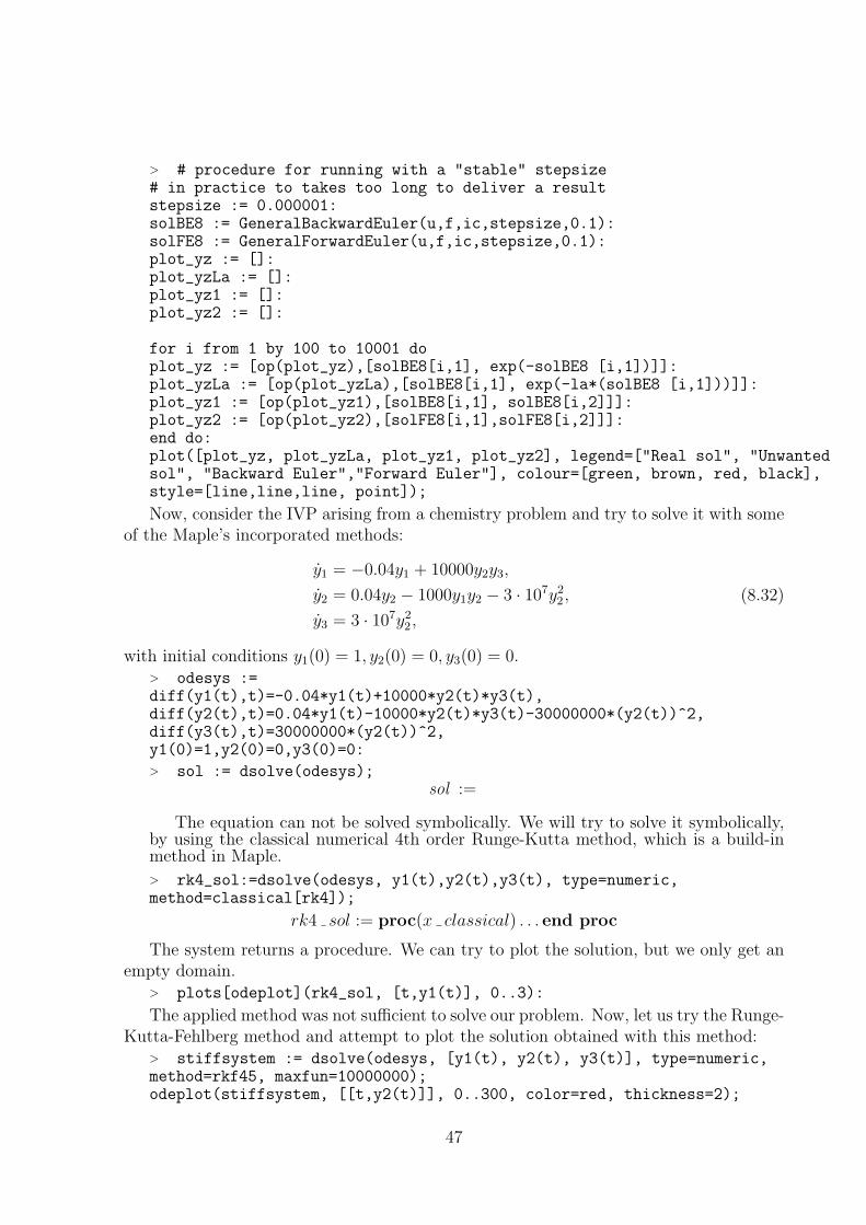
> # procedure for running with a "stable" stepsize# in practice to takes too long to deliver a resultstepsize := 0.000001:solBE8 := GeneralBackwardEuler(u,f,ic,stepsize,0.1):solFE8 := GeneralForwardEuler(u,f,ic,stepsize,0.1):plot_yz := []:plot_yzLa := []:plot_yz1 := []:plot_yz2 := []:

for i from 1 by 100 to 10001 doplot_yz := [op(plot_yz),[solBE8[i,1], exp(-solBE8 [i,1])]]:plot_yzLa := [op(plot_yzLa),[solBE8[i,1], exp(-la*(solBE8 [i,1]))]]:plot_yz1 := [op(plot_yz1),[solBE8[i,1], solBE8[i,2]]]:plot_yz2 := [op(plot_yz2),[solFE8[i,1],solFE8[i,2]]]:end do:plot([plot_yz, plot_yzLa, plot_yz1, plot_yz2], legend=["Real sol", "Unwantedsol", "Backward Euler","Forward Euler"], colour=[green, brown, red, black],style=[line,line,line, point]);

Now, consider the IVP arising from a chemistry problem and try to solve it with someof the Maple’s incorporated methods:

y1 = −0.04y1 + 10000y2y3,

y2 = 0.04y2 − 1000y1y2 − 3 · 107y22,

y3 = 3 · 107y22,

(8.32)

with initial conditions y1(0) = 1, y2(0) = 0, y3(0) = 0.> odesys :=diff(y1(t),t)=-0.04*y1(t)+10000*y2(t)*y3(t),diff(y2(t),t)=0.04*y1(t)-10000*y2(t)*y3(t)-30000000*(y2(t))^2,diff(y3(t),t)=30000000*(y2(t))^2,y1(0)=1,y2(0)=0,y3(0)=0:> sol := dsolve(odesys);

sol :=

The equation can not be solved symbolically. We will try to solve it symbolically,by using the classical numerical 4th order Runge-Kutta method, which is a build-inmethod in Maple.

> rk4_sol:=dsolve(odesys, y1(t),y2(t),y3(t), type=numeric,method=classical[rk4]);

rk4 sol := proc(x classical) . . . end proc

The system returns a procedure. We can try to plot the solution, but we only get anempty domain.

> plots[odeplot](rk4_sol, [t,y1(t)], 0..3):

The applied method was not sufficient to solve our problem. Now, let us try the Runge-Kutta-Fehlberg method and attempt to plot the solution obtained with this method:

> stiffsystem := dsolve(odesys, [y1(t), y2(t), y3(t)], type=numeric,method=rkf45, maxfun=10000000);odeplot(stiffsystem, [[t,y2(t)]], 0..300, color=red, thickness=2);

47

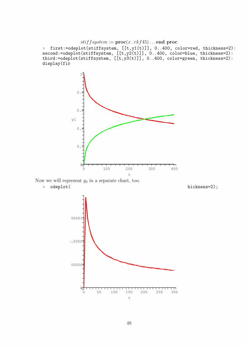
stiffsystem := proc(x rkf45) . . . end proc> first:=odeplot(stiffsystem, [[t,y1(t)]], 0..400, color=red, thickness=2):second:=odeplot(stiffsystem, [[t,y2(t)]], 0..400, color=blue, thickness=2):third:=odeplot(stiffsystem, [[t,y3(t)]], 0..400, color=green, thickness=2):display(first,second,third);

y1

0.8

0

1

0.6

t

4003001000

0.2

0.4

200

Now we will represent y2 in a separate chart, too.> odeplot(stiffsystem, [[t,y2(t)]], 0..300, color=red, thickness=2);

0.000005

0.000015

0.00001

0

t

300250150100 200500

48

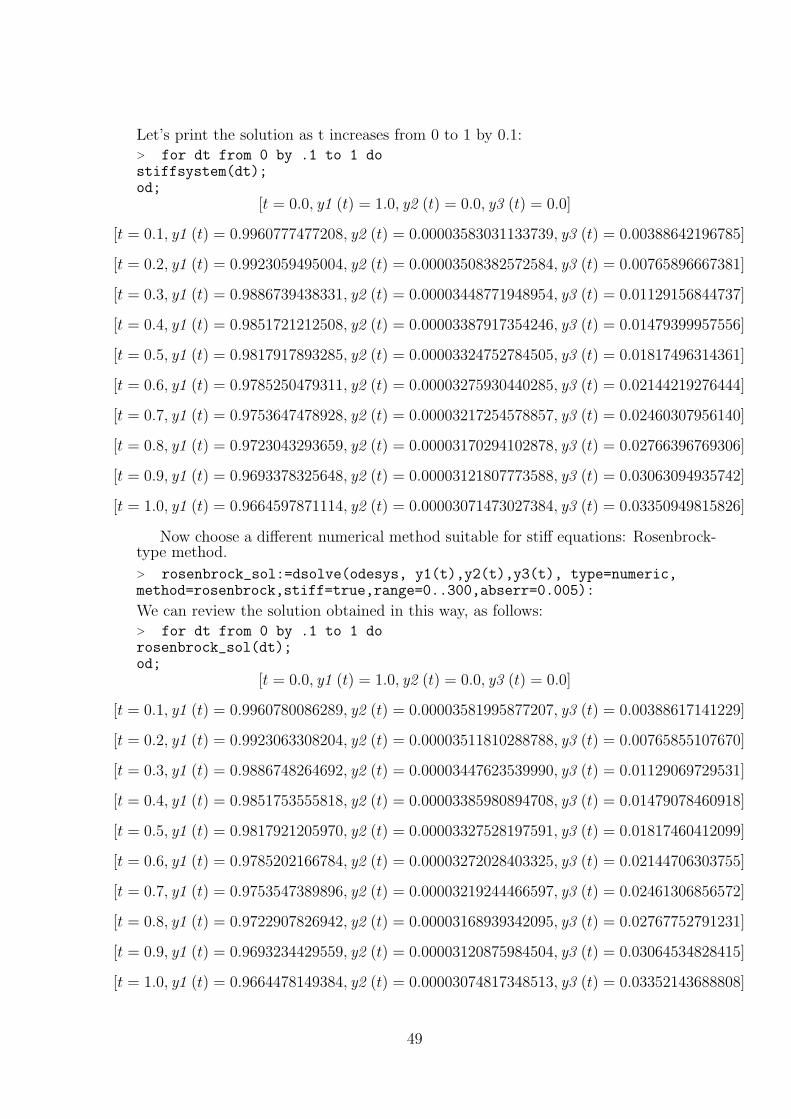
Let’s print the solution as t increases from 0 to 1 by 0.1:> for dt from 0 by .1 to 1 dostiffsystem(dt);od;

[t = 0.0, y1 (t) = 1.0, y2 (t) = 0.0, y3 (t) = 0.0]

[t = 0.1, y1 (t) = 0.9960777477208, y2 (t) = 0.00003583031133739, y3 (t) = 0.00388642196785]

[t = 0.2, y1 (t) = 0.9923059495004, y2 (t) = 0.00003508382572584, y3 (t) = 0.00765896667381]

[t = 0.3, y1 (t) = 0.9886739438331, y2 (t) = 0.00003448771948954, y3 (t) = 0.01129156844737]

[t = 0.4, y1 (t) = 0.9851721212508, y2 (t) = 0.00003387917354246, y3 (t) = 0.01479399957556]

[t = 0.5, y1 (t) = 0.9817917893285, y2 (t) = 0.00003324752784505, y3 (t) = 0.01817496314361]

[t = 0.6, y1 (t) = 0.9785250479311, y2 (t) = 0.00003275930440285, y3 (t) = 0.02144219276444]

[t = 0.7, y1 (t) = 0.9753647478928, y2 (t) = 0.00003217254578857, y3 (t) = 0.02460307956140]

[t = 0.8, y1 (t) = 0.9723043293659, y2 (t) = 0.00003170294102878, y3 (t) = 0.02766396769306]

[t = 0.9, y1 (t) = 0.9693378325648, y2 (t) = 0.00003121807773588, y3 (t) = 0.03063094935742]

[t = 1.0, y1 (t) = 0.9664597871114, y2 (t) = 0.00003071473027384, y3 (t) = 0.03350949815826]

Now choose a different numerical method suitable for stiff equations: Rosenbrock-type method.

> rosenbrock_sol:=dsolve(odesys, y1(t),y2(t),y3(t), type=numeric,method=rosenbrock,stiff=true,range=0..300,abserr=0.005):

We can review the solution obtained in this way, as follows:> for dt from 0 by .1 to 1 dorosenbrock_sol(dt);od;

[t = 0.0, y1 (t) = 1.0, y2 (t) = 0.0, y3 (t) = 0.0]

[t = 0.1, y1 (t) = 0.9960780086289, y2 (t) = 0.00003581995877207, y3 (t) = 0.00388617141229]

[t = 0.2, y1 (t) = 0.9923063308204, y2 (t) = 0.00003511810288788, y3 (t) = 0.00765855107670]

[t = 0.3, y1 (t) = 0.9886748264692, y2 (t) = 0.00003447623539990, y3 (t) = 0.01129069729531]

[t = 0.4, y1 (t) = 0.9851753555818, y2 (t) = 0.00003385980894708, y3 (t) = 0.01479078460918]

[t = 0.5, y1 (t) = 0.9817921205970, y2 (t) = 0.00003327528197591, y3 (t) = 0.01817460412099]

[t = 0.6, y1 (t) = 0.9785202166784, y2 (t) = 0.00003272028403325, y3 (t) = 0.02144706303755]

[t = 0.7, y1 (t) = 0.9753547389896, y2 (t) = 0.00003219244466597, y3 (t) = 0.02461306856572]

[t = 0.8, y1 (t) = 0.9722907826942, y2 (t) = 0.00003168939342095, y3 (t) = 0.02767752791231]

[t = 0.9, y1 (t) = 0.9693234429559, y2 (t) = 0.00003120875984504, y3 (t) = 0.03064534828415]

[t = 1.0, y1 (t) = 0.9664478149384, y2 (t) = 0.00003074817348513, y3 (t) = 0.03352143688808]

49

A graphical representation of the solution can be obtained via the following commands:> first’:=plots[odeplot](rosenbrock_sol, [t,y1(t)], 0..300, color=red):> second’:=plots[odeplot](rosenbrock_sol, [t,y2(t)], 0..300, color=blue,thickness=2):> third’:=plots[odeplot](rosenbrock_sol, [t,y3(t)], 0..300, color=green,thickness=2):> plots[display](first’, second’, third’);

y1

0.8

0

1

0.6

t

300250150100

0.2

0.4

2000 50

Another alternative to solve the stiff system may be the use of the Livermore ODEsolver based on backward differentiation formulas. The solution was depicted in this caseas well.

> stiff back := dsolve(odesys, y1(t), y2(t), y3(t), type=numeric,method=lsode[backfull]);odeplot(stiff back, [[t,y1(t)],[t,y2(t)],[t,y3(t)]], 0..300, color=green,thickness=2);

stiff back := proc(x lsode) . . . end proc

50

y1, y2, y3

0.8

0

1

0.6

t

300250150100

0.2

0.4

2000 50

References

[Ado94] G. Adomian, Solving Frontier Problems of Physics: The Decomposition Method,Kluwer Academic Publishers, Boston, MA, 1994.

[Ala07] M. Alabdullatif, H. A. Abdusalam, E. S. Fahmy, Adomian decomposition methodfor nonlinear reaction diffusion system of Lotka-Volterra type, International Mathe-matical Forum, 2, 2007, no. 2, 87–96.

[Aro96] C. J. Aro, CHEMSODE: a stiff ODE solver for the equations of chemical kinetics,Computer Physics Communications 97 (1996) 304–314.

[Ber96] E. Bertolazzi, Positive and Conservative Schemes for Mass Action Kinetics, Com-puters Math. Applic. Vol. 32, No. 6, pp. 29–43, 1996.

[Bia06] J. Biazar, M. Pourabd, A Maple program for computing Adomian polynomials,International Mathematical Forum, 1, 2006, no. 39, 1919-1924.

[Cab] M. Caberlin, N. Nigam, S. Qazi, Invariant manifolds in a model for the GABAreceptorhttp://www.math.mcgill.ca/nigam/MAIN/pub/caberlin nigam qazi.pdf

51

[Cli96] L. J. Clifford, A. M. Milne, B. A. Murray, Numerical modeling of Chemistry anGas Dynamics During Shock-Induced Ethylene Combustion Combustion and Flame104; 311–327, 1996, Elsevier Science Inc.

[Dam02] V. Damian, A. Sandu, M. Damian, F. Potra, G. R. Carmichael, The kineticpreprocessor KPP–a software environment for solving chemical kinetics, Computersand Chemical Engineering 26 (2002) 1567–1579.

[Dit06] P. Dita, N. Grama, On Adomians Decomposition Method for Solving DifferentialEquations,arXiv:solv-int/9705008 1, May 24, 2006,http://arxiv.org/PS cache/solv-int/pdf/9705/9705008.pdf

[Edw97] J. T. Edwards, J. A. Roberts, N. J. Ford, A comparison of Adomian’s decompo-sition method and Runge Kutta methods for approximate solution of some predatorprey model eqautions, Numerical Analysis Report no. 309, October 1997.

[Fed97] R. P. Fedkiw, B. Merriman, S. Osher, High Accuracy Numerical Methods forThermally Perfect Gas Flows with Chemistry, Journal of Computational Physics,132, 175-190 (1997) article no. CP965622.

[Kay04] D. Kaya A reliable method for the numerical solution of the kinetics problems,Appl. Math. Comput. 156 (2004) 261-270.

[Kno98] O. Knoth, R. Wolke, Implicit-explicit Runge-Kutta methods for computing atmo-spheric reactive flows, Applied Numerital Mathematics 28 (1998) 327–341.

[Lam85] S. H. Lam, Singular perturbation for stiff equations using numerical methods,Recent Advances in the Aerospace Sciences, Corrado Casci, Ed., Plenum Press, NewYork and London, pp.3–20, 1985.

[Lam93] S. H. Lam, Using CSP to Understand Complex Chemical Kinetics, CombustionScience and Technology, 89, 5–6, pp. 375, 1993.

[Lam94] S. H. Lam, D. A. Goussis, The CSP Method for Simplifying Kinetics, Interna-tional Journal of Chemical Kinetics 26, pp. 461–486, 1994.

[Lam95] S. H. Lam, Reduced Chemistry Modeling and Sensitivity Analysis, Lecture notesfor Aerothermochemistry for Hypersonic Technology, 1994-1995,http://www.princeton.edu/∼lam/SHL/VKI.pdf

[Lor99] R. Lorenzini, L. Passoni, Test of numerical methods for the integration of kineticequations in tropospheric chemistry, Computer Physics Communications 117 (1999)241–249.

[Pre88] http://www.library.cornell.edu/nr/cbookcpdf.html

[Rae02] M. Rae, M. N. Berberan-Santos, Pre-equilibrium approximation in chemical andphotophysical kinetics, Chemical Physics 280 (2002) 283-293.

52

[San97] A. Sandu, J. G. Verwer, M. Van Loon, G. R. Carmichael, F. A. Potra, D. Dabdub,J. H. Seinfeld, Benchmarking stiff ode solvers for atmospheric chemistry problems-I. Implicit vs explicit, Athmospheric Environment, Vol. 31, No. 19, pp. 3151–3166,1997.

[Say95] R. D. Saylor, G. D. Ford, On the comparison of numerical methods for the inte-gration of kinetic equations in atmospheric chemistry and transport models, Athmo-spheric Environment, Vol. 29, No. 19, pp. 2585-2593, 1995.

[Ver95] J. G. Verwer, D. Simpson, Explicit methods for stiff ODEs from atmosphericchemistry, Applied Numerical Mathematics 18 (1995) 413–430.

[Ver97] J. G. Verwer, E.J. Spee, J.G. Blom, W. Hundsdorfer, A Second Order RosenbrockMethod Applied to Photochemical Dispersion Problems, Report MAS-R9717, August31, 1997,http://ftp.cwi.nl/CWIreports/MAS/MAS-R9717.pdf

[Vos01] D. A. Voss, A. Q. M. Khaliq, Parallel Rosenbrock methods for chemical systems,Computers and Chemistry 25 (2001) 101-107.

53