DOCSIS 4.0 - A Key Ingredient of the 2030's Broadband Pie

© 2021, SCTE® CableLabs® and NCTA. All rights reserved. 1

DOCSIS 4.0 - A Key Ingredient of the 2030's Broadband Pie

A Technical Paper prepared for SCTE by

Zoran Maricevic, Ph.D. Engineering Fellow

CommScope Wallingford, CT 203-303-6547

[email protected]

James Andis

General Manager – HFC Technologies | CTO Networks, Engineering & Security (NES)

nbn™ Australia Melbourne, Victoria - Australia

+61 409 066 745 [email protected]

Tom Cloonan, Ph.D. Chief Technology Officer

CommScope Lisle, IL

630-281-3050 [email protected]

John Ulm

Engineering Fellow CommScope

Moultonborough, NH 978-609-6028

[email protected]


Table of Contents Title Page Number

1. Introduction .......................................................................................................................................... 4 2. Network Evolution: Drivers and Timing ............................................................................................... 6

2.1. The 10GTM Initiative ................................................................................................................ 6 2.2. Traffic Engineering For the Future ......................................................................................... 6 2.3. Some Potential Future Service Tier Use Cases .................................................................... 7

3. Network Evolution: Various Paths Considered ................................................................................. 13 3.1. Baseline – an N+5 node area to start from .......................................................................... 13 3.2. Network evolution options .................................................................................................... 14 3.3. N+2 and N+0 upgrade options ............................................................................................. 14

4. Network Evolution: Total Cost of Ownership Compared................................................................... 17 4.1. Network upgrade paths considered ..................................................................................... 17 4.2. Capital Expenditures (CAPEX) ............................................................................................ 18 4.3. Operating Expenditures (OPEX) .......................................................................................... 19 4.4. Total Cost of Ownership (TCO) ............................................................................................ 20 4.5. Sensitivity Analysis - CAPEX ............................................................................................... 21 4.6. Sensitivity Analysis - OPEX ................................................................................................. 22 4.7. Sensitivity Analysis – TCO ................................................................................................... 24 4.8. Will network capacity gains justify various upgrade costs? ................................................. 25 4.9. TCO analysis Takeaways .................................................................................................... 27 4.10. Scenarios in which going straight to FTTP/PON makes more sense .................................. 27 4.11. Greenfield scenarios – business as usual or FTTP/PON? .................................................. 29

5. Discussion – The Steps to Get There ............................................................................................... 29 5.1. The name of the game is optionality .................................................................................... 29

6. Conclusions ....................................................................................................................................... 32 Abbreviations .............................................................................................................................................. 34 Bibliography & References.......................................................................................................................... 35


List of Figures Title Page Number Figure 1 – The nbnTM Residential FTTP journey ........................................................................................... 4 Figure 2 – Past Downstream and Upstream Average Bandwidth Usage Trends ......................................... 8 Figure 3 – Future Downstream and Upstream Average Bandwidth Usage Predictions ............................... 8 Figure 4 – Future Downstream and Upstream Maximum Service Level Agreement Trends ....................... 9 Figure 5 – 1794/300 MHz migration with 8G x 2G Service Tier, 120 subs/SG .......................................... 10 Figure 6 – 1794/492 MHz migration with 6G x 3G Service Tier, 120 subs/SG .......................................... 10 Figure 7 – 1794/300 MHz migration with 10G x 2G Service Tier, 60 subs/SG .......................................... 12 Figure 8 – 1794/492 MHz migration with 7.5G x 3.5G Service Tier, 60 subs/SG ...................................... 12 Figure 9 – HFC area under study, 945 HP, uneven distribution across node ports ................................... 13 Figure 10 – Possible future evolution path directions for a typical HFC network ....................................... 14 Figure 11 – Single node area under study converted from N+5 to N+2 topology ...................................... 15 Figure 12 – Single node area converted from N+5 to N+0 “fiber-deep” topology ....................................... 15 Figure 13 – Percentage of New Fiber + Coax required for various Upgrade Options ................................ 16 Figure 14 – Overview of Upgrade elements considered in CAPEX calculation ......................................... 17 Figure 15 – Network upgraded from I-CCAP to DAA ................................................................................. 17 Figure 16 – Normalized CAPEX in $/HP for each upgrade paths .............................................................. 18 Figure 17 – 15-year Normalized OPEX, in $/HP, for each upgrade path ................................................... 19 Figure 18 – Field actives failure over time, for estimating maintenance cost ............................................. 20 Figure 19 – 15-year Normalized TCO, in $/HP, for each upgrade path ..................................................... 20 Figure 20 – Monte-Carlo variability and sensitivity analysis of CAPEX for CCAP N+5 .............................. 21 Figure 21 – Monte-Carlo variability and sensitivity analysis of CAPEX for ESD N+5 ................................ 22 Figure 22 – Monte-Carlo variability and sensitivity analysis of CAPEX for 10G R-PON ............................ 22 Figure 23 – OPEX variability of PON upgrades and HFC upgrades .......................................................... 23 Figure 24 – OPEX sensitivity analysis for PON and HFC upgrades .......................................................... 23 Figure 25 – CAPEX + OPEX variability adding to that of TCO variability ................................................... 24 Figure 26 – Sensitivity of ESD N+5 Total Cost to the various assumptions and their ranges .................... 24 Figure 27 – Year 2021 DS/US top tier rates enabled by the 9 upgrade paths (FDX, ESD presumed not

yet available) ....................................................................................................................................... 25 Figure 28 – Year 2036 DS/US top tier rates enabled by 9 upgrade paths; mid-split US out of gas ........... 26 Figure 29 – Year 2036 DS/US top tier rates enabled by 9 upgrade paths; high-split in the 1st three ........ 26 Figure 30 – An example of preexisting cell-tower fiber routes, with "dark fiber" strands available to

support FTTP/PON .............................................................................................................................. 28

List of Tables Title Page Number Table 1 – How HFC network attribute change with upgrading N+5 area to N+2 and N+0 ......................... 16 Table 2 – Network upgrade scenarios considered ..................................................................................... 18


1. Introduction There is no doubt that Fiber to the Premise (FTTP) is the very long-term end goal of every operator. The questions of when and how to move to FTTP within a cable brownfield is the billion-dollar question. It is widely recognized that FTTP is expected to cost more than a comparable upgrade to DOCSIS 4.0 using Extended Spectrum DOCSIS (ESD) – yet both will yield similar speed tiers and revenue from a residential service perspective during the 2030’s and into the early 2040’s.

In Australia, nbnTM (National Broadband Network) is a government-business enterprise that has recently completed the rollout of a ubiquitous broadband network. This national broadband network is leveraging copper, coax, fiber, Fixed Wireless and Satellite assets, and has used a truly technology agnostic approach to servicing 100% of the population. Like other operators in the post-COVID world, nbn is driving its broadband infrastructure efficiently to meet traffic demands and expected performance, and nbn has one of the most extensive DOCSIS 3.1 deployments in the world. Coupled with fully segmented (4x4) nodes over a fully analogue forward and return path architecture, nbn is now evaluating what the next significant investment cycle, expected in 2025/26, will entail and is asking the hard question as to whether this is the right time to overbuild FTTP to every residential home or to do another round of DOCSIS investments using Distributed Access Architectures (DAA) and DOCSIS 4.0.

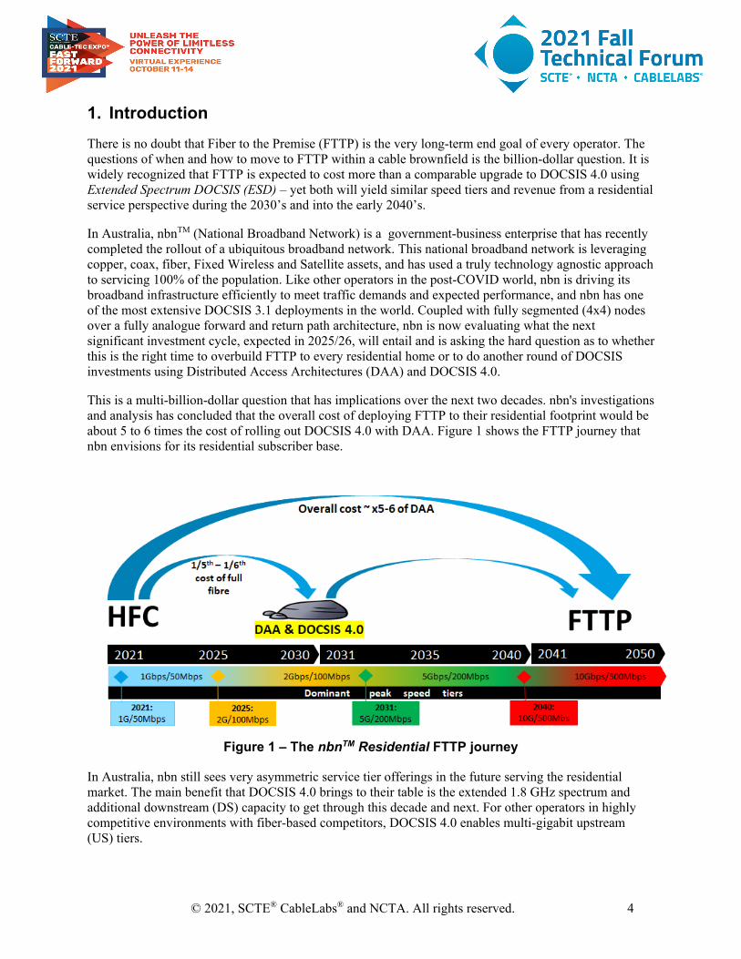
This is a multi-billion-dollar question that has implications over the next two decades. nbn's investigations and analysis has concluded that the overall cost of deploying FTTP to their residential footprint would be about 5 to 6 times the cost of rolling out DOCSIS 4.0 with DAA. Figure 1 shows the FTTP journey that nbn envisions for its residential subscriber base.

Figure 1 – The nbnTM Residential FTTP journey

In Australia, nbn still sees very asymmetric service tier offerings in the future serving the residential market. The main benefit that DOCSIS 4.0 brings to their table is the extended 1.8 GHz spectrum and additional downstream (DS) capacity to get through this decade and next. For other operators in highly competitive environments with fiber-based competitors, DOCSIS 4.0 enables multi-gigabit upstream (US) tiers.


For the next 5-10 years, nbn will be prioritizing major uplifts to FTTP in area’s served by copper infrastructure (Fiber-to-the-Node/FTTN), namely, to address demand for higher speed services (> 50 Mbps or > 100 Mbps) which come with associated revenue uplifts and ceases further investment in copper remediation required to maintain the network. These copper areas will utilize existing Distribution Fiber Network (DFN) that nbn has already deployed to serve the DSLAM nodes, essentially extending the fiber deeper to pass all the premises served by the copper Distribution Area (DA). Fiber drops to homes will be built when customers order services of 100 Mbps or more; essentially using a demand driven approach.

Unlike copper-based services, nbn’s HFC services do not suffer from the inability to reach Gigabit speeds or require intense and expensive remediation activities to maintain those speeds. For this reason, there is no major uplift in revenue expected from offloading HFC services to FTTP. When coupled with the recent large scale DOCSIS 3.1 investment and deployment, the nbn HFC network has adequate headroom in capacity to defer the next major investment cycle for several years.

There is no doubt that fully symmetric services will become an important offering for business in the near future. Fibre based 1 G and 10 G Ethernet are commonly deployed for businesses as well. However, DOCSIS-based alternatives with lower deployment costs might also have a great appeal - to business customers and operators alike.

For operators, DOCSIS 4.0 is a compelling proposition. It allows them to remain competitive, by delivering reliable high-speed residential services well into the 2030’s across a wide footprint. As an interim technology, it allows operators to strategically deploy deep-fibre and FTTP where needed, while enabling the evolution of the HFC network towards N+0/N+1/N+2 DAA deployments. The reality is that most operators don’t have the funds and resources to deploy FTTP to every customer in a short time frame – this is evident from the efforts of many companies who have attempted full fibre overbuilds.

This paper provides a case study of possible network evolution steps on an actual node; and then looks at the Total Cost of Ownership (TCO) for each option. This will show others the same steps that nbn went through in their decision-making process. The three approaches considered are:

• Full FTTP overbuild and offload. • DOCSIS 4.0 Extended Spectrum DOCSIS (ESD) using DAA • A hybrid approach - where deep-fibre DOCSIS 4.0 DAA deployments are coupled with

selective/targeted FTTP offloads – to provide an optimum outcome that minimizes upfront CAPEX and maximizes the longevity of operator Investments in the DOCSIS part of network

The paper also considers network power consumption, material and truck roll costs for actives, passives, fiber and coax maintenance, as well as for the drop line maintenance and replacement, and give overview on how to make estimates for the costs over an extended period of performance.

The net present value (NPV) of the expected OPEX savings is the dollars-and-sense measuring stick against the investments required to achieve the savings - similar to calculating a payoff for a solar-powered home system without giving credit to all the environmental benefits. (Going green while collecting greens, that is.)


2. Network Evolution: Drivers and Timing

2.1. The 10GTM Initiative

The 10G Initiative within the Cable Industry is a key focal point for future vendor product developments and for future Multiple System Operator (MSO) architectural plans. At a high level, 10G defines the simple goal of providing 10 Gbps to subscribers in the future. In addition to speed increases, 10G also defines important goals of improving latency, security, and reliability within future Cable Industry service platforms. As a result, 10G will undoubtedly drive innovation on many fronts into the Cable Industry.

The upcoming arrival of DOCSIS 4.0 equipment (both Full Duplex, FDX, and Extended Spectrum DOCSIS, ESD) within the next few years will mark the next step in the quest for 10G - with a focus on providing the bandwidth via HFC plant augmentations. Since DOCSIS 4.0 equipment deployments will begin in the near future, it is imperative that we begin studying the timing and magnitude of the associated bandwidth capacity needs to ensure that the DOCSIS 4.0 equipment can support the required bandwidths.

These future capacity needs are being partially driven by subscriber demands (higher average bandwidth consumption resulting from higher resolution IP Video and larger subscriber numbers). But as we move forward towards 10G services, the biggest drivers for 10G operation will likely materialize from market challenges instead of subscriber demands. These challenges may result from competitor technologies that are capable of offering service level agreements (SLA) with bandwidths exceeding the typical maximum SLA of 1 Gbps offered by many Multiple System Operators (MSOs) today. Last-mile technologies that may be competitive to DOCSIS over the next 10-15 years include Passive Optical Networks (PON), 5G wireless/fixed wireless, and satellite services.

Satellite services are becoming more ubiquitous with more broadband-oriented, low-earth orbit satellites being launched on a regular basis. However, large latencies (due to the lengthy round-trip path) and relatively low bandwidth capacities (< 100 Mbps) would likely preclude these systems from competing with fiber and DOCSIS in a high-bandwidth marketing war of the future [SATELLITE].

5G wireless/fixed wireless can potentially offer competitive bandwidth capacities, and it has much more bandwidth capacity than satellite services. For sub-6 GHz 5G operations, capacities are expected to reach 500 Mbps. However, mmWave 5G technologies using 24-39 GHz ranges could offer 1.5 Gbps service level agreements or higher that could leap-frog the current DOCSIS 1 Gbps capacity [FORBES]. Limitations in current DOCSIS upstream capacity may be another area where fixed wireless service providers may attack.

PON is the most competitive to DOCSIS of these last-mile technologies. Several variants of PON already support 10 Gbps services. These include 10G EPON (10G x 10G), XG-PON (10G x 2.5G), XGS-PON (10G x 10G), NG-PON2 (multiple 10G lambdas), and NG-EPON (25G x 25G or 50G x 50G) [ITU]. Coherent PON services are also being studied that may eventually support even higher capacities.

Thus, 5G and PON are both technologies that could launch capacity-oriented marketing campaigns against DOCSIS in the coming years. It may prove beneficial to use forward-looking estimates of likely bandwidth capacity rollouts to predict when DOCSIS 4.0 augmentations may be required in the future.

2.2. Traffic Engineering For the Future

Previously, [CLO_2014] introduced traffic engineering and quality of experience (QoE) for broadband networks. From there, the paper went on to develop a relatively simple traffic engineering formula for


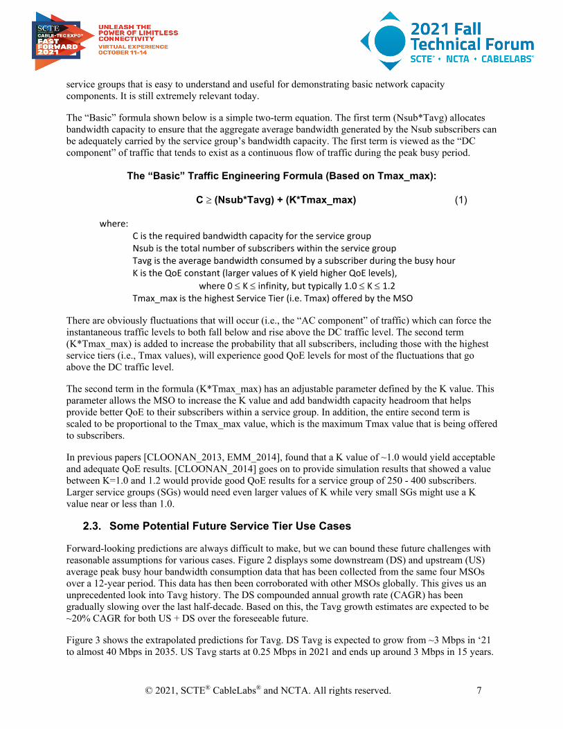
service groups that is easy to understand and useful for demonstrating basic network capacity components. It is still extremely relevant today.

The “Basic” formula shown below is a simple two-term equation. The first term (Nsub*Tavg) allocates bandwidth capacity to ensure that the aggregate average bandwidth generated by the Nsub subscribers can be adequately carried by the service group’s bandwidth capacity. The first term is viewed as the “DC component” of traffic that tends to exist as a continuous flow of traffic during the peak busy period.

The “Basic” Traffic Engineering Formula (Based on Tmax_max):

C ≥ (Nsub*Tavg) + (K*Tmax_max) (1)

where: C is the required bandwidth capacity for the service group Nsub is the total number of subscribers within the service group Tavg is the average bandwidth consumed by a subscriber during the busy hour K is the QoE constant (larger values of K yield higher QoE levels),

where 0 ≤ K ≤ infinity, but typically 1.0 ≤ K ≤ 1.2 Tmax_max is the highest Service Tier (i.e. Tmax) offered by the MSO

There are obviously fluctuations that will occur (i.e., the “AC component” of traffic) which can force the instantaneous traffic levels to both fall below and rise above the DC traffic level. The second term (K*Tmax_max) is added to increase the probability that all subscribers, including those with the highest service tiers (i.e., Tmax values), will experience good QoE levels for most of the fluctuations that go above the DC traffic level.

The second term in the formula (K*Tmax_max) has an adjustable parameter defined by the K value. This parameter allows the MSO to increase the K value and add bandwidth capacity headroom that helps provide better QoE to their subscribers within a service group. In addition, the entire second term is scaled to be proportional to the Tmax_max value, which is the maximum Tmax value that is being offered to subscribers.

In previous papers [CLOONAN_2013, EMM_2014], found that a K value of ~1.0 would yield acceptable and adequate QoE results. [CLOONAN_2014] goes on to provide simulation results that showed a value between K=1.0 and 1.2 would provide good QoE results for a service group of 250 - 400 subscribers. Larger service groups (SGs) would need even larger values of K while very small SGs might use a K value near or less than 1.0.

2.3. Some Potential Future Service Tier Use Cases

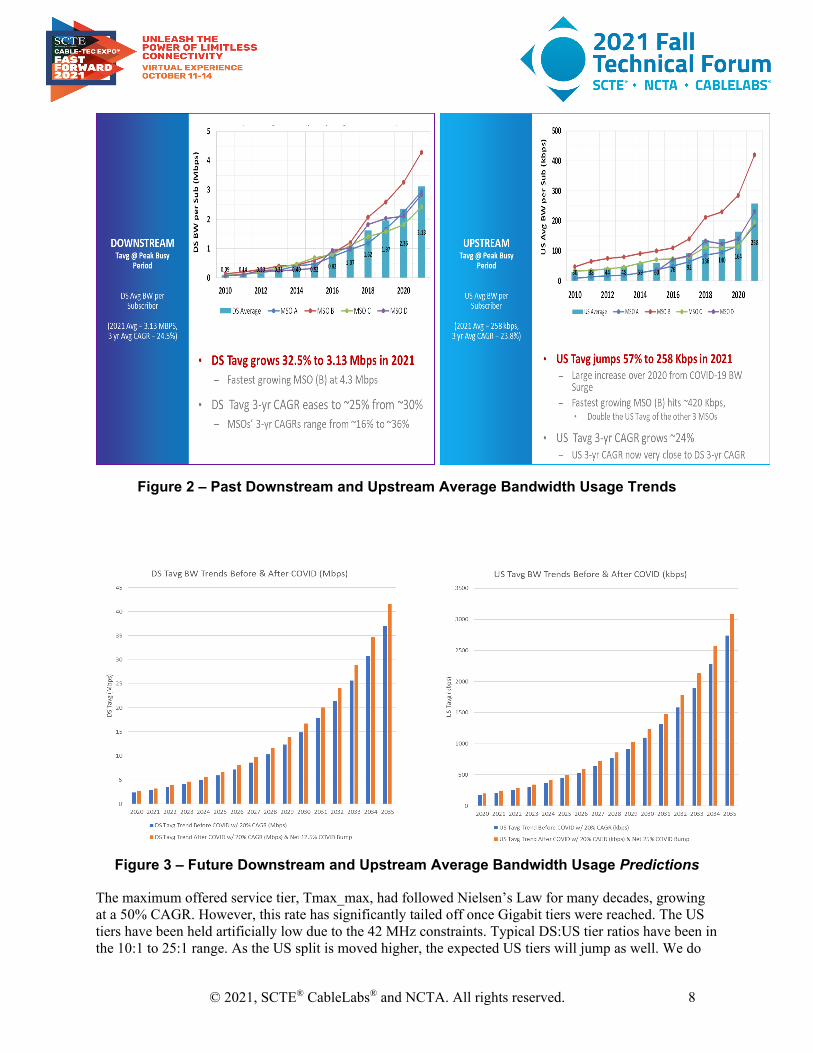
Forward-looking predictions are always difficult to make, but we can bound these future challenges with reasonable assumptions for various cases. Figure 2 displays some downstream (DS) and upstream (US) average peak busy hour bandwidth consumption data that has been collected from the same four MSOs over a 12-year period. This data has then been corroborated with other MSOs globally. This gives us an unprecedented look into Tavg history. The DS compounded annual growth rate (CAGR) has been gradually slowing over the last half-decade. Based on this, the Tavg growth estimates are expected to be ~20% CAGR for both US + DS over the foreseeable future.

Figure 3 shows the extrapolated predictions for Tavg. DS Tavg is expected to grow from ~3 Mbps in ‘21 to almost 40 Mbps in 2035. US Tavg starts at 0.25 Mbps in 2021 and ends up around 3 Mbps in 15 years.


Figure 2 – Past Downstream and Upstream Average Bandwidth Usage Trends

Figure 3 – Future Downstream and Upstream Average Bandwidth Usage Predictions

The maximum offered service tier, Tmax_max, had followed Nielsen’s Law for many decades, growing at a 50% CAGR. However, this rate has significantly tailed off once Gigabit tiers were reached. The US tiers have been held artificially low due to the 42 MHz constraints. Typical DS:US tier ratios have been in the 10:1 to 25:1 range. As the US split is moved higher, the expected US tiers will jump as well. We do


not expect it to become fully 1:1 symmetric, but rather a much closer 2:1 to 4:1 ratio of DS to US. Going forward, it is estimated that Tmax_max will double roughly every five years for an effective 15% CAGR. This is shown in Figure 4.

Figure 4 – Future Downstream and Upstream Maximum Service Level Agreement Trends

Previously, [ULM_2019] discussed how a 1218/204 MHz plant can support a 10G migration over the ‘20s decade. The 1218/204 MHz upgrade is still a strong viable option for networks needing immediate bandwidth capacity relief. However, with DOCSIS 4.0 products becoming closer to reality, some operators are wondering if they can get by with existing plants and then make a giant leap up to a 1794 MHz ESD plant. The CommScope Network Capacity Planning model that leverages the QoE-based Traffic Engineering formula helped us analyze several interesting use cases as the network migrates from 860 to 1794 MHz.

For our analysis, the timeframe is extended out 15 years, to 2035. The network starts with 300 MHz of legacy video spectrum and 30 bonded DOCSIS 3.0 SC-QAM channels. By 2033, the legacy video spectrum is removed in favor of IPTV over DOCSIS. Also, by this time, all 2.0/3.0 modems are assumed to be removed such that the network is now 100% OFDM/OFDMA channels. The model uses an effective DS OFDM bit rate of 8.8 bps/Hz and an US OFDMA bit rate of 7.7 bps/Hz.

The first two use cases shown in Figures 5 and 6 are for a CMTS Service Group (SG) with 120 subscribers (e.g., 240 HP, Homes Passed, @ 50% penetration). The next two use cases in Figures 7 and 8 assume a much smaller 60 subs per SG that an MSO might see from a fiber deep deployment.


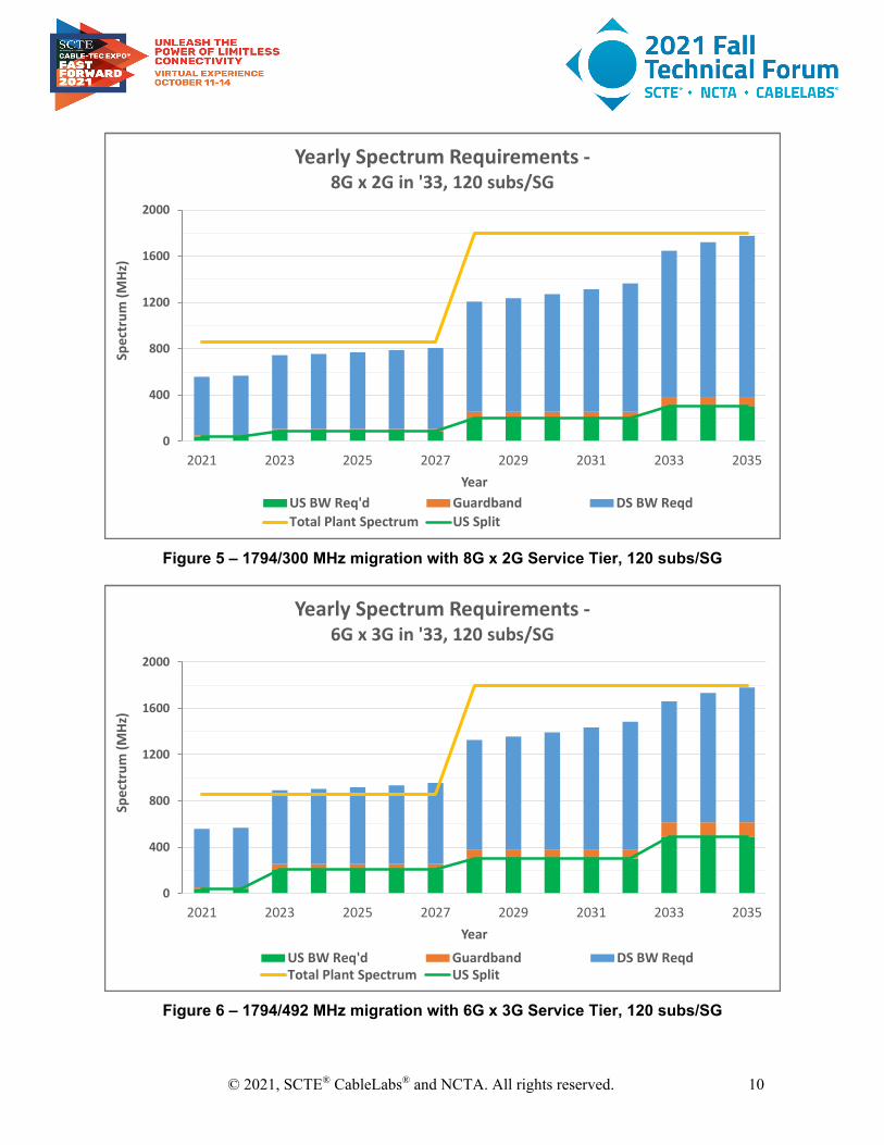
Figure 5 – 1794/300 MHz migration with 8G x 2G Service Tier, 120 subs/SG


0

400

800

1200

1600

2000

2021 2023 2025 2027 2029 2031 2033 2035

Spec

trum

(MHz

)

Year

Yearly Spectrum Requirements -8G x 2G in '33, 120 subs/SG

US BW Req'd Guardband DS BW ReqdTotal Plant Spectrum US Split

0

400

800

1200

1600

2000

2021 2023 2025 2027 2029 2031 2033 2035

Spec

trum

(MHz

)

Year




The use case in Figure 5 assumes a 4:1 DS:US ratio with 120 subs/SG. The max service tier progresses to 2G x 500M, 4G x 1G and finally 8G x 2G. The 860/85 MHz plant can carry the operator through 2027. In 2028, the introduction of the 1G US tier forces an upgrade to 204 MHz at which time the downstream is also upgraded to 1.8 GHz. Note that a 1218 MHz plant would still be viable through the end of the decade. By 2033, the 2G US tier requires the US split to be changed to 300 MHz. Room is made for the 8G DS tier by the IPTV savings and removal of 2.0/3.0 SC-QAMs. By 2035, both the US + DS spectrum are filling up for this SG size.

Operators will need to install DOCSIS 4.0 equipment prior to enabling it, because the installation of the various components may take years. That installed equipment may be operated in a DOCSIS 3.1 mode for a while before being configured to enable DOCSIS 4.0 bandwidth capacities whenever the needs arise. Also note that some existing “1GHz” taps can actually operate at much higher frequencies. Depending on the tap type, they may not need to be replaced until the year 2033 jump in service tiers. This would give the operator a 12-year window to make the tap replacements.

The use case in Figure 6 assumes a 2:1 DS:US ratio with 120 subs/SG. The max service tier progresses to 2G x 1G, 4G x 2G and finally 6G x 3G. This use case requires a 204 MHz US split once the 1G US tier is introduced. An 860/204 MHz plant can be stretched for a couple more years by using the roll-off region above 860 MHz. Note that only the limited number of 2G subscribers might need to infrequently use that roll-off bandwidth. By 2028, the introduction of the 4G x 2G tier forces the network to upgrade to 1794/300 MHz. Later, the 3G US tier causes the US split to move to 492 MHz. This reduces available DS spectrum which is why the DS tier is limited to 6G.

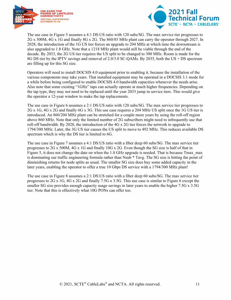
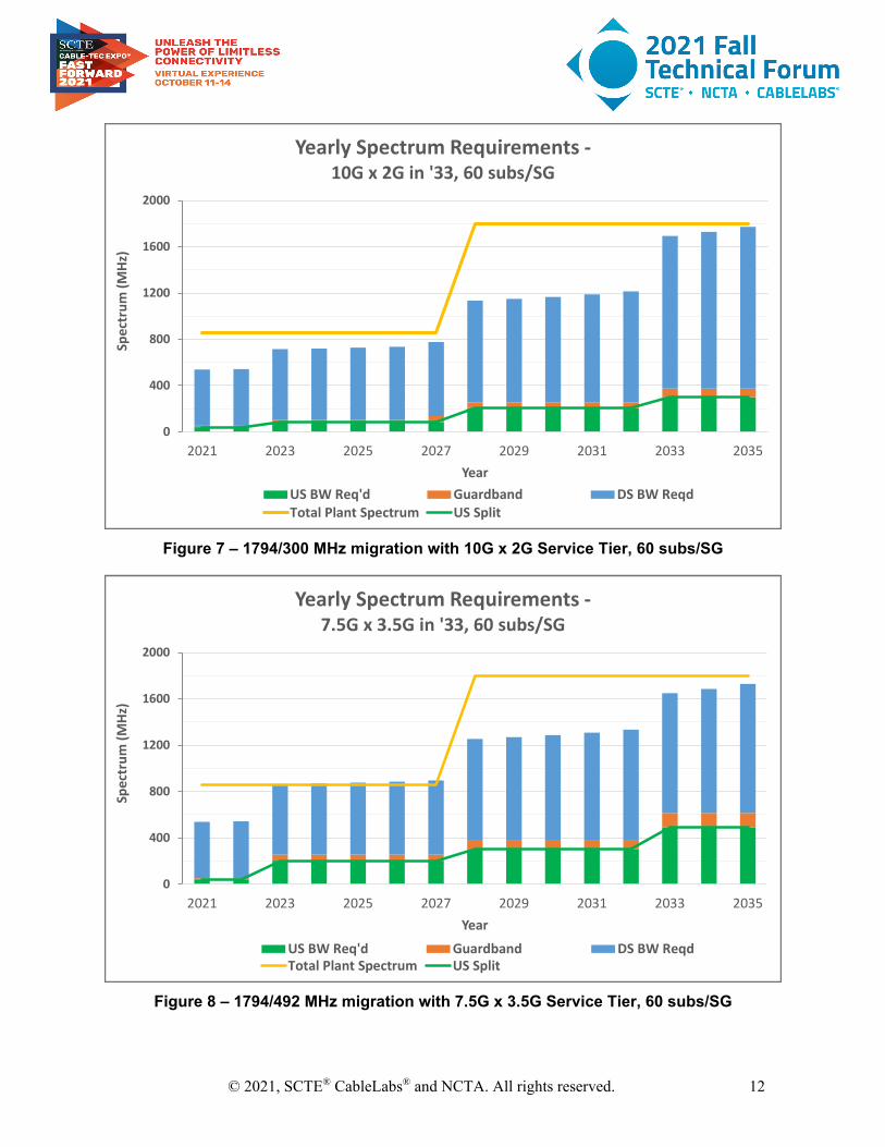
The use case in Figure 7 assumes a 4:1 DS:US ratio with a fiber deep 60 subs/SG. The max service tier progresses to 2G x 500M, 4G x 1G and finally 10G x 2G. Even though the SG size is half of that in Figure 5, it does not change the date on when the 1.8 GHz upgrade is needed. That is because Tmax_max is dominating our traffic engineering formula rather than Nsub * Tavg. The SG size is hitting the point of diminishing returns for node splits as usual. The smaller SG size does buy some added capacity in the later years, enabling the operator to offer a true 10 Gbps DS service with a 1794/300 MHz plant!

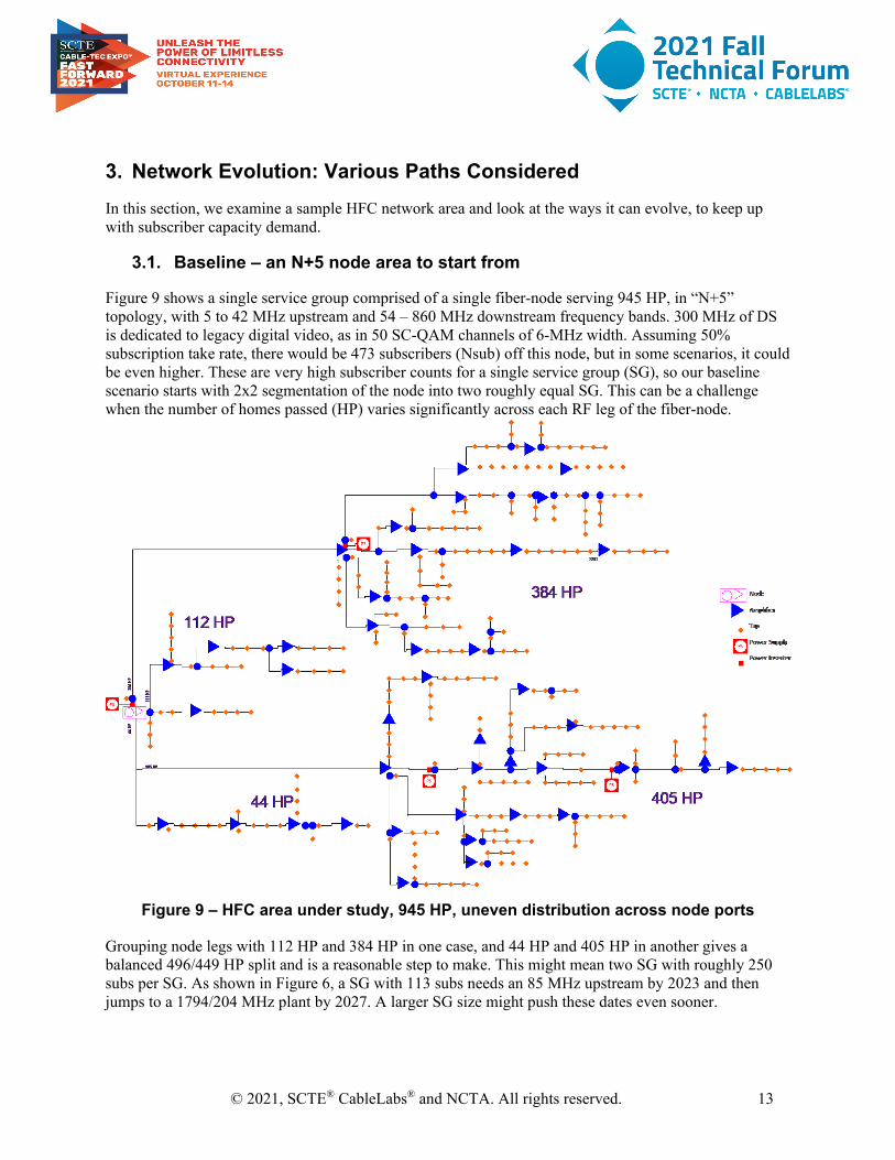
The use case in Figure 8 assumes a 2:1 DS:US ratio with a fiber deep 60 subs/SG. The max service tier progresses to 2G x 1G, 4G x 2G and finally 7.5G x 3.5G. This use case is similar to Figure 6 except the smaller SG size provides enough capacity usage savings in later years to enable the higher 7.5G x 3.5G tier. Note that this is effectively what 10G PONs can offer too.



Figure 8 – 1794/492 MHz migration with 7.5G x 3.5G Service Tier, 60 subs/SG

0

400

800

1200

1600

2000

2021 2023 2025 2027 2029 2031 2033 2035

Spec

trum

(MHz

)

Year



0

400

800

1200

1600

2000

2021 2023 2025 2027 2029 2031 2033 2035

Spec

trum

(MHz

)

Year

Yearly Spectrum Requirements -7.5G x 3.5G in '33, 60 subs/SG



3. Network Evolution: Various Paths Considered In this section, we examine a sample HFC network area and look at the ways it can evolve, to keep up with subscriber capacity demand.

3.1. Baseline – an N+5 node area to start from

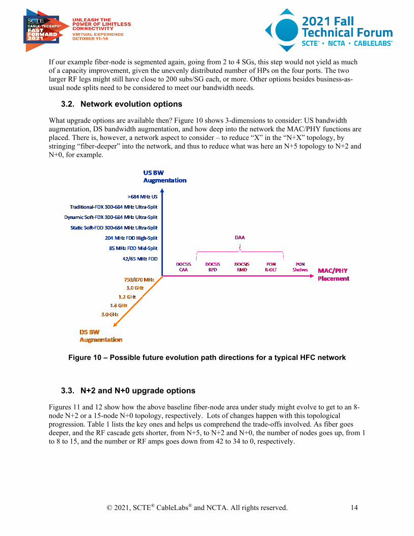
Figure 9 shows a single service group comprised of a single fiber-node serving 945 HP, in “N+5” topology, with 5 to 42 MHz upstream and 54 – 860 MHz downstream frequency bands. 300 MHz of DS is dedicated to legacy digital video, as in 50 SC-QAM channels of 6-MHz width. Assuming 50% subscription take rate, there would be 473 subscribers (Nsub) off this node, but in some scenarios, it could be even higher. These are very high subscriber counts for a single service group (SG), so our baseline scenario starts with 2x2 segmentation of the node into two roughly equal SG. This can be a challenge when the number of homes passed (HP) varies significantly across each RF leg of the fiber-node.

Figure 9 – HFC area under study, 945 HP, uneven distribution across node ports

Grouping node legs with 112 HP and 384 HP in one case, and 44 HP and 405 HP in another gives a balanced 496/449 HP split and is a reasonable step to make. This might mean two SG with roughly 250 subs per SG. As shown in Figure 6, a SG with 113 subs needs an 85 MHz upstream by 2023 and then jumps to a 1794/204 MHz plant by 2027. A larger SG size might push these dates even sooner.


If our example fiber-node is segmented again, going from 2 to 4 SGs, this step would not yield as much of a capacity improvement, given the unevenly distributed number of HPs on the four ports. The two larger RF legs might still have close to 200 subs/SG each, or more. Other options besides business-as-usual node splits need to be considered to meet our bandwidth needs.

3.2. Network evolution options

What upgrade options are available then? Figure 10 shows 3-dimensions to consider: US bandwidth augmentation, DS bandwidth augmentation, and how deep into the network the MAC/PHY functions are placed. There is, however, a network aspect to consider – to reduce “X” in the “N+X” topology, by stringing “fiber-deeper” into the network, and thus to reduce what was here an N+5 topology to N+2 and N+0, for example.

Figure 10 – Possible future evolution path directions for a typical HFC network

3.3. N+2 and N+0 upgrade options

Figures 11 and 12 show how the above baseline fiber-node area under study might evolve to get to an 8-node N+2 or a 15-node N+0 topology, respectively. Lots of changes happen with this topological progression. Table 1 lists the key ones and helps us comprehend the trade-offs involved. As fiber goes deeper, and the RF cascade gets shorter, from N+5, to N+2 and N+0, the number of nodes goes up, from 1 to 8 to 15, and the number or RF amps goes down from 42 to 34 to 0, respectively.


Figure 11 – Single node area under study converted from N+5 to N+2 topology

Figure 12 – Single node area converted from N+5 to N+0 “fiber-deep” topology


Repositioning of actives also causes changes to the taps: 34 out of 286 need a new faceplate for N+2 while as many as 208 out of 286 taps need the same for N+0. A 1.9 miles portion of the hardline coax needs fiber overlash for N+2, and as many of 6.5 miles of new coax/fiber for N+0. As a result, the distance from the furthest subscriber to the nearest fiber point/node reduces from 7,000 to 2,500 and 1,600 feet away, for N+5, N+2 and N+0 respectively.

Table 1 – How HFC network attribute change with upgrading N+5 area to N+2 and N+0 Topology: N+5 N+2 N+0

Number of Standard Nodes 1 8 15 Number of RF amps 42 34 0 Number of tap faceplate changes out of # of taps 0/ 286 15/ 286 208/ 286 New plant; miles/ % 0 1.9 miles/ 19% 6.5 miles/ 67% Fiber to the last subscriber <7,000 ft <2,500 ft <1,600 ft

Note, this is an important point to consider for a future FTTP evolution. Installing new fiber is beneficial, in the sense that it gets the operator closer to the goal of getting fiber all the way to the customer premise. Figure 13 shows what percentage of the hardline plant gets over-lashed with fiber for various N+X scenarios: N+5, N+2, N+1, N+0, fiber to the last active (FTTLA) and fiber to the tap (FTTT), with some of these explained in detail in reference [Venk_SCTE_2016]

Figure 13 – Percentage of New Fiber + Coax required for various Upgrade Options

However, installing new fiber can be a costly proposition. This is especially true when dealing with underground plant that does not have any preinstalled conduits and thus where substantial digging and trenching is required. How does this cost compare to making improvements along the three dimensions shown in Figure 10? That is what the next section considers.


4. Network Evolution: Total Cost of Ownership Compared To make sense of the myriad of tradeoffs involved, we present a simplified “total cost of ownership” (TCO) model for various upgrade options. Figure 14 shows an overview of the access network elements accounted for in this cost exercise, as well as a starting point from which to migrate this 5-42 MHz upstream, 54-860 MHz downstream, I-CCAP network. Furthermore, the taps in the network are assumed to need a faceplate upgrade for 1.2 GHz and a complete tap upgrade for 1.8 GHz.

Figure 14 – Overview of Upgrade elements considered in CAPEX calculation

If the topology were to change from N+5 to N+2 or to N+0, the field portion of the network would get upgraded. The field portion would change from that in Figure 9 to that of Figures 11 and 12, respectively. If the I-CCAP were to get converted to DAA, the left-hand portion of Figure 14 would change to that of Figure 15.

Figure 15 – Network upgraded from I-CCAP to DAA

4.1. Network upgrade paths considered

The nine upgrade scenarios analyzed are shown in Table 2. The names were selected for brevity, so they correspond to labels in the resulting plots. Other elements of the table include: architecture type (i.e. centralized I-CCAP, distributed DAA and PON), number of serving groups (SG), homes passed per SG (HP/SG) and number of nodes. The RF split and top DS frequencies, if applicable, are also shown.


Table 2 – Network upgrade scenarios considered

Name Architecture # of SG HP/SG # of nodes RF split DS BW

CCAP N+5 I-CCAP 2 ~480 2 Mid or high 1,218 MHz CCAP N+2 I-CCAP 4 ~240 8 Mid or high 1,218 MHz CCAP N+0 I-CCAP 4 ~240 15 Mid or high 1,218 MHz FDX N+0 DAA 4 ~240 15 108-684 1,218 MHz FDX-Lite N+5 DAA 2 ~480 2 108-396 1,218 MHz ESD N+5 DAA 2 ~480 2 396/492 UHS 1,794 MHz ESD N+2 DAA 4 ~240 8 396/492 UHS 1,794 MHz 10G PON OLT in hub 15 64 N.A. N.A. N.A. 10G R-PON OLT in node 8 128 N.A. N.A. N.A.

4.2. Capital Expenditures (CAPEX)

Figure 16 shows the one-time capital expenditures (CAPEX) for each of the options. These are then normalized to the highest-cost case – that of the 10G Remote-OLT PON (R-PON). The legend shows a breakout for various cost components. On the headend side, there are CMTS (or OLT if PON) and head-end optics (HEO) – which includes SFPs for DAA and PON. On the field side, categories are: node hardware; field hardware consisting of RF amplifiers and fiber enclosures; labor expense to install nodes/amplifiers/fiber enclosures; then new fiber, material and labor; and taps, material and labor (or splitters, material and labor, if PON). On the customer premise side drops, material and labor and CPE – the ONUs for PON – are included.

Figure 16 – Normalized CAPEX in $/HP for each of 9 upgrade paths

For I-CCAP, each service group gets 32x4 DSxUS D3.0 SC-QAM channels and 192x48 MHz DSxUS wide OFDM/A D3.1 channels. For DAA, it’s 32x4 DSxUS D3.0 SC-QAM channels and 192x96 MHz DSxUS wide OFDM/A D3.1 or D4.0 channels. The fiber – material & construction labor estimates - shown in orange, are dominant in some upgrade cases and are based on $2 per foot for aerial and $12 per


foot for underground, with 80/20% mix of aerial/underground assumed, for a blended cost of $4 per foot. For CCAP N+5 and N+2, only the RF amplifier modules get replaced while the housings remain as they are. For all other cases which contain RF amplifiers, the complete old housing cutout and replacement with a whole new RF amplifier station is assumed. For FDX N+5, ESD N+5 and N+2 cases, given that no FDX nor ESD field RF hardware exists yet, a 40% HW cost premium is assumed over a comparable 1.2 GHz RF amplifier unit. For the PON cases, only the cost of subscriber drops and ONU hardware and install is included – which represents 50% of homes-passed - in order not to overburden PON CAPEX estimates.

4.3. Operating Expenditures (OPEX)

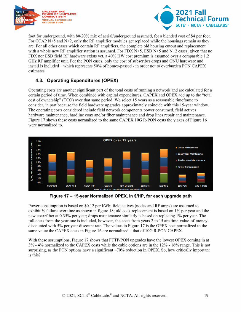
Operating costs are another significant part of the total costs of running a network and are calculated for a certain period of time. When combined with capital expenditures, CAPEX and OPEX add up to the “total cost of ownership” (TCO) over that same period. We select 15 years as a reasonable timeframe to consider, in part because the field hardware upgrades approximately coincide with this 15-year window. The operating costs considered include field network components power consumed, field actives hardware maintenance, hardline coax and/or fiber maintenance and drop lines repair and maintenance. Figure 17 shows these costs normalized to the same CAPEX 10G R-PON costs the y axes of Figure 16 were normalized to.

Figure 17 – 15-year Normalized OPEX, in $/HP, for each upgrade path

Power consumption is based on $0.12 per kWh; field actives (nodes and RF amps) are assumed to exhibit % failure over time as shown in figure 18; old coax replacement is based on 1% per year and the new coax/fiber at 0.35% per year; drops maintenance similarly is based on replacing 1% per year. The full costs from the year one is included, however, the costs from years 2 to 15 are time-value-of-money discounted with 5% per year discount rate. The values in Figure 17 is the OPEX cost normalized to the same value the CAPEX costs in Figure 16 are normalized – that of 10G R-PON CAPEX.

With these assumptions, Figure 17 shows that FTTP/PON upgrades have the lowest OPEX coming in at 3% - 4% normalized to the CAPEX costs while the cable options are in the 12% - 16% range. This is not surprising, as the PON options have a significant ~70% reduction in OPEX. So, how critically important is this?


Figure 18 – Field actives failure over time, for estimating maintenance cost

4.4. Total Cost of Ownership (TCO)

The answer is provided by adding CAPEX and OPEX together, resulting in the TCO, as shown in Figure 19. At a first glance, no free lunch opportunity is detected, because those low operating expenses for the PON upgrades sit on the top of a very tall “candlestick” of the PON capital expenses. Nevertheless, TCO ratios did significantly reduce, as compared to those of CAPEX: take 10G R-PON vs. ESD N+5 for example: the CAPEX ratio was ~6, while the TCO ratio is down to ~3.

Figure 19 – 15-year Normalized TCO, in $/HP, for each upgrade path

Figure 19 gives the impression that staying with longer cascades (N+5) is the lower cost thing to do, as compared to progressively more expensive N+2, N+0 and FTTP. However, this does not consider the


potential network capacity gains from the other options. Would the network capacity gained justify these additional upgrade costs? The answer to this question is in a later section. However, let’s first consider why should one trust these comparisons and numbers anyhow?

There are many factors that go into calculating TCO with many associated assumptions. Isn’t there a way to give the reader some additional insights into the assumptions made, and what happens if those assumptions are changed? Monte-Carlo variability analysis comes to the rescue – and to getting these questions answered.

4.5. Sensitivity Analysis - CAPEX

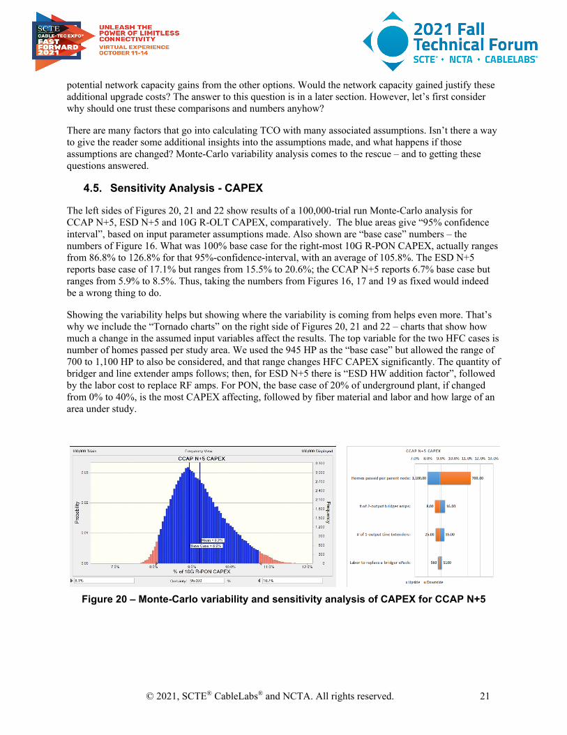
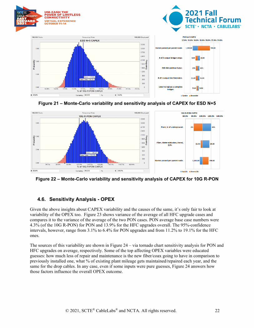
The left sides of Figures 20, 21 and 22 show results of a 100,000-trial run Monte-Carlo analysis for CCAP N+5, ESD N+5 and 10G R-OLT CAPEX, comparatively. The blue areas give “95% confidence interval”, based on input parameter assumptions made. Also shown are “base case” numbers – the numbers of Figure 16. What was 100% base case for the right-most 10G R-PON CAPEX, actually ranges from 86.8% to 126.8% for that 95%-confidence-interval, with an average of 105.8%. The ESD N+5 reports base case of 17.1% but ranges from 15.5% to 20.6%; the CCAP N+5 reports 6.7% base case but ranges from 5.9% to 8.5%. Thus, taking the numbers from Figures 16, 17 and 19 as fixed would indeed be a wrong thing to do.

Showing the variability helps but showing where the variability is coming from helps even more. That’s why we include the “Tornado charts” on the right side of Figures 20, 21 and 22 – charts that show how much a change in the assumed input variables affect the results. The top variable for the two HFC cases is number of homes passed per study area. We used the 945 HP as the “base case” but allowed the range of 700 to 1,100 HP to also be considered, and that range changes HFC CAPEX significantly. The quantity of bridger and line extender amps follows; then, for ESD N+5 there is “ESD HW addition factor”, followed by the labor cost to replace RF amps. For PON, the base case of 20% of underground plant, if changed from 0% to 40%, is the most CAPEX affecting, followed by fiber material and labor and how large of an area under study.

Figure 20 – Monte-Carlo variability and sensitivity analysis of CAPEX for CCAP N+5


Figure 21 – Monte-Carlo variability and sensitivity analysis of CAPEX for ESD N+5

Figure 22 – Monte-Carlo variability and sensitivity analysis of CAPEX for 10G R-PON

4.6. Sensitivity Analysis - OPEX

Given the above insights about CAPEX variability and the causes of the same, it’s only fair to look at variability of the OPEX too. Figure 23 shows variance of the average of all HFC upgrade cases and compares it to the variance of the average of the two PON cases. PON average base case numbers were 4.3% (of the 10G R-PON) for PON and 13.9% for the HFC upgrades overall. The 95%-confidence intervals, however, range from 3.1% to 6.4% for PON upgrades and from 11.2% to 19.1% for the HFC ones.

The sources of this variability are shown in Figure 24 – via tornado chart sensitivity analysis for PON and HFC upgrades on average, respectively. Some of the top affecting OPEX variables were educated guesses: how much less of repair and maintenance is the new fiber/coax going to have in comparison to previously installed one, what % of existing plant mileage gets maintained/repaired each year, and the same for the drop cables. In any case, even if some inputs were pure guesses, Figure 24 answers how those factors influence the overall OPEX outcome.


Figure 23 – OPEX variability of PON upgrades and HFC upgrades

Figure 24 – OPEX sensitivity analysis for PON and HFC upgrades


4.7. Sensitivity Analysis – TCO

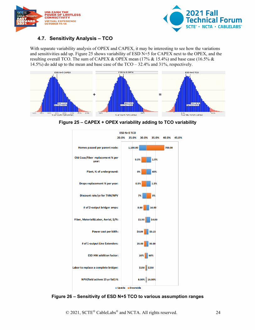
With separate variability analysis of OPEX and CAPEX, it may be interesting to see how the variations and sensitivities add up. Figure 25 shows variability of ESD N+5 for CAPEX next to the OPEX, and the resulting overall TCO. The sum of CAPEX & OPEX mean (17% & 15.4%) and base case (16.5% & 14.5%) do add up to the mean and base case of the TCO – 32.4% and 31%, respectively.

Figure 25 – CAPEX + OPEX variability adding to TCO variability

Figure 26 – Sensitivity of ESD N+5 TCO to various assumption ranges


The most contributing assumptions to the overall variability of ESD N+5 TCO are shown in the “tornado chart” in figure 26. The divisor of homes-passed per parent node features prominently, primarily because of the wide 700 - 1,100 HP range considered, as compared to the fixed 945 HP in the node area under study. Five other factors are OPEX; the rest are CAPEX driven. Hardline coax % replaced, 0.5% to 1.5% range per year, is the next most contributing, the % of underground plant enters via cost of old coax replacement – more costly if more underground; and so on.

The above sensitivity analysis, done by introducing variability into model’s assumptions and then detecting what changes and by how much in the model’s outputs, helped us gauge the reasonableness of the modeling process. That was but one of the ways of keeping “GIGO” (Garbage In, Garbage Out) from affecting our reasoning. The other way was to “keep it sophisticatedly simple (KISS), but not too simplistic”. Thus, KISS and no-GIGO were our guiding principles in making these models.

4.8. Will network capacity gains justify various upgrade costs?

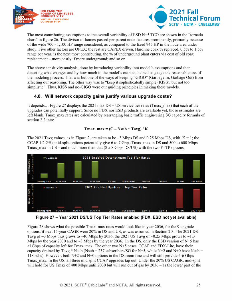
It depends… Figure 27 displays the 2021 max DS + US service tier rates (Tmax_max) that each of the upgrades can potentially support. Since no FDX nor ESD products are available yet, those estimates are left blank. Tmax_max rates are calculated by rearranging basic traffic engineering SG capacity formula of section 2.2 into:

Tmax_max = (C – Nsub * Tavg) / K

The 2021 Tavg values, as in Figure 2, are taken to be ~3 Mbps DS and 0.25 Mbps US, with K = 1; the CCAP 1.2 GHz mid-split options potentially give 6 to 7 Gbps Tmax_max in DS and 500 to 600 Mbps Tmax_max in US – and much more than that (8 x 8 Gbps DS/US) with the two FTTP options.

Figure 27 – Year 2021 DS/US Top Tier Rates enabled (FDX, ESD not yet available)

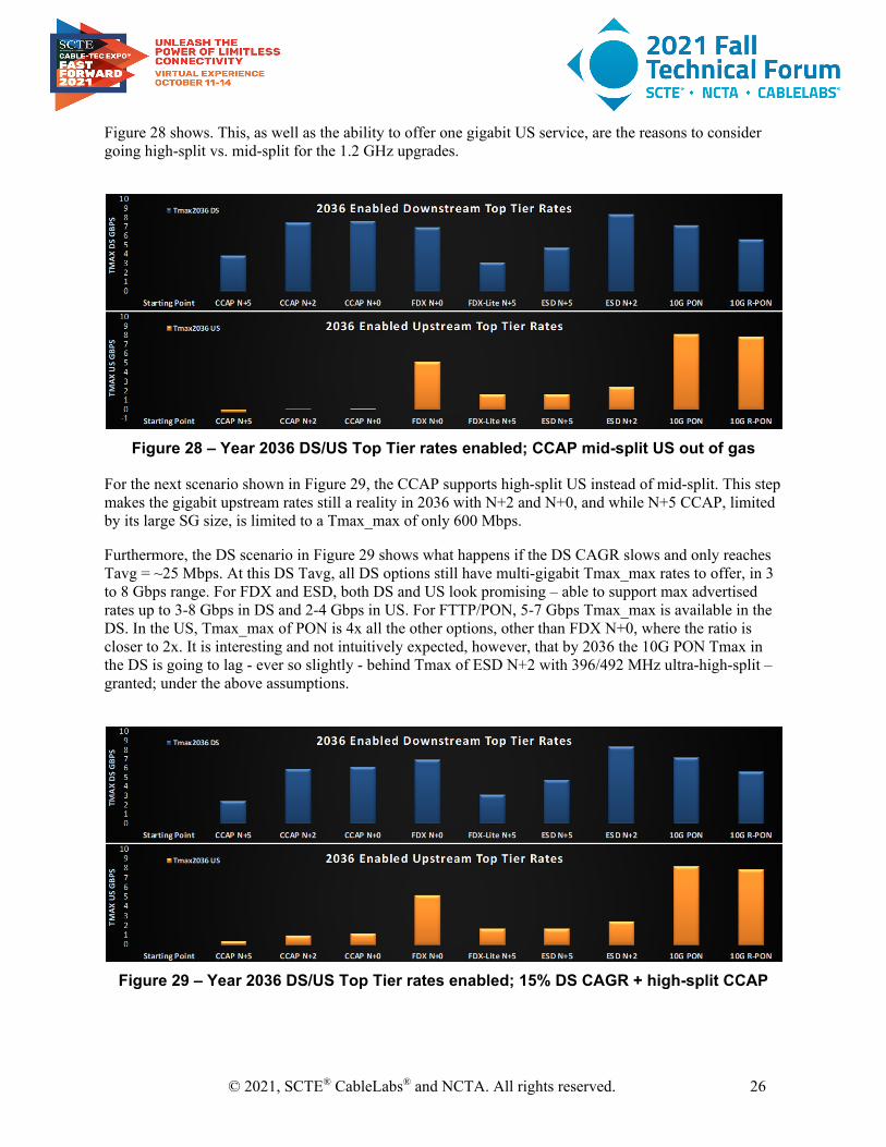
Figure 28 shows what the possible Tmax_max rates would look like in year 2036, for the 9 upgrade options, if next 15-year CAGR were 20% in DS and US, as was assumed in Section 2.3. The 2021 DS Tavg of ~3 Mbps thus grows to ~40 Mbps by 2036, the 2021 US Tavg of ~0.25 Mbps grows to ~1.3 Mbps by the year 2030 and to ~3 Mbps by the year 2036. In the DS, only the ESD version of N+5 has >1Gbps of capacity left for Tmax_max. The other two N+5 cases, CCAP and FDX-Lite, have their capacity drained by Tavg * Nsub (Nsub = 237 subscribers/SG for N+5, while N+2 and N+0 have Nsub = 118 subs). However, both N+2 and N+0 options in the DS seem fine and will still provide 5-6 Gbps Tmax_max. In the US, all three mid split CCAP upgrades tap out. Under the 20% US CAGR, mid-split will hold for US Tmax of 400 Mbps until 2030 but will run out of gas by 2036 – as the lower part of the


Figure 28 shows. This, as well as the ability to offer one gigabit US service, are the reasons to consider going high-split vs. mid-split for the 1.2 GHz upgrades.

Figure 28 – Year 2036 DS/US Top Tier rates enabled; CCAP mid-split US out of gas

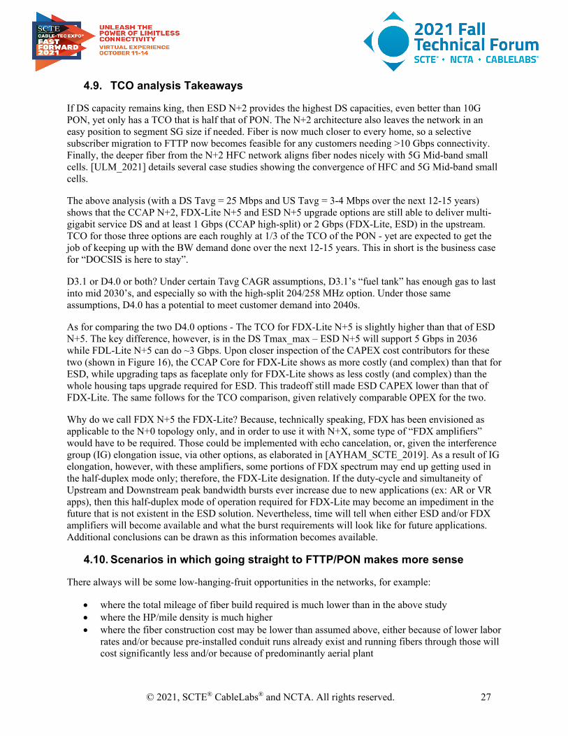
For the next scenario shown in Figure 29, the CCAP supports high-split US instead of mid-split. This step makes the gigabit upstream rates still a reality in 2036 with N+2 and N+0, and while N+5 CCAP, limited by its large SG size, is limited to a Tmax_max of only 600 Mbps.

Furthermore, the DS scenario in Figure 29 shows what happens if the DS CAGR slows and only reaches Tavg = ~25 Mbps. At this DS Tavg, all DS options still have multi-gigabit Tmax_max rates to offer, in 3 to 8 Gbps range. For FDX and ESD, both DS and US look promising – able to support max advertised rates up to 3-8 Gbps in DS and 2-4 Gbps in US. For FTTP/PON, 5-7 Gbps Tmax_max is available in the DS. In the US, Tmax_max of PON is 4x all the other options, other than FDX N+0, where the ratio is closer to 2x. It is interesting and not intuitively expected, however, that by 2036 the 10G PON Tmax in the DS is going to lag - ever so slightly - behind Tmax of ESD N+2 with 396/492 MHz ultra-high-split – granted; under the above assumptions.

Figure 29 – Year 2036 DS/US Top Tier rates enabled; 15% DS CAGR + high-split CCAP


4.9. TCO analysis Takeaways

If DS capacity remains king, then ESD N+2 provides the highest DS capacities, even better than 10G PON, yet only has a TCO that is half that of PON. The N+2 architecture also leaves the network in an easy position to segment SG size if needed. Fiber is now much closer to every home, so a selective subscriber migration to FTTP now becomes feasible for any customers needing >10 Gbps connectivity. Finally, the deeper fiber from the N+2 HFC network aligns fiber nodes nicely with 5G Mid-band small cells. [ULM_2021] details several case studies showing the convergence of HFC and 5G Mid-band small cells.

The above analysis (with a DS Tavg = 25 Mbps and US Tavg = 3-4 Mbps over the next 12-15 years) shows that the CCAP N+2, FDX-Lite N+5 and ESD N+5 upgrade options are still able to deliver multi-gigabit service DS and at least 1 Gbps (CCAP high-split) or 2 Gbps (FDX-Lite, ESD) in the upstream. TCO for those three options are each roughly at 1/3 of the TCO of the PON - yet are expected to get the job of keeping up with the BW demand done over the next 12-15 years. This in short is the business case for “DOCSIS is here to stay”.

D3.1 or D4.0 or both? Under certain Tavg CAGR assumptions, D3.1’s “fuel tank” has enough gas to last into mid 2030’s, and especially so with the high-split 204/258 MHz option. Under those same assumptions, D4.0 has a potential to meet customer demand into 2040s.

As for comparing the two D4.0 options - The TCO for FDX-Lite N+5 is slightly higher than that of ESD N+5. The key difference, however, is in the DS Tmax_max – ESD N+5 will support 5 Gbps in 2036 while FDL-Lite N+5 can do ~3 Gbps. Upon closer inspection of the CAPEX cost contributors for these two (shown in Figure 16), the CCAP Core for FDX-Lite shows as more costly (and complex) than that for ESD, while upgrading taps as faceplate only for FDX-Lite shows as less costly (and complex) than the whole housing taps upgrade required for ESD. This tradeoff still made ESD CAPEX lower than that of FDX-Lite. The same follows for the TCO comparison, given relatively comparable OPEX for the two.

Why do we call FDX N+5 the FDX-Lite? Because, technically speaking, FDX has been envisioned as applicable to the N+0 topology only, and in order to use it with N+X, some type of “FDX amplifiers” would have to be required. Those could be implemented with echo cancelation, or, given the interference group (IG) elongation issue, via other options, as elaborated in [AYHAM_SCTE_2019]. As a result of IG elongation, however, with these amplifiers, some portions of FDX spectrum may end up getting used in the half-duplex mode only; therefore, the FDX-Lite designation. If the duty-cycle and simultaneity of Upstream and Downstream peak bandwidth bursts ever increase due to new applications (ex: AR or VR apps), then this half-duplex mode of operation required for FDX-Lite may become an impediment in the future that is not existent in the ESD solution. Nevertheless, time will tell when either ESD and/or FDX amplifiers will become available and what the burst requirements will look like for future applications. Additional conclusions can be drawn as this information becomes available.

4.10. Scenarios in which going straight to FTTP/PON makes more sense

There always will be some low-hanging-fruit opportunities in the networks, for example:

• where the total mileage of fiber build required is much lower than in the above study • where the HP/mile density is much higher • where the fiber construction cost may be lower than assumed above, either because of lower labor

rates and/or because pre-installed conduit runs already exist and running fibers through those will cost significantly less and/or because of predominantly aerial plant


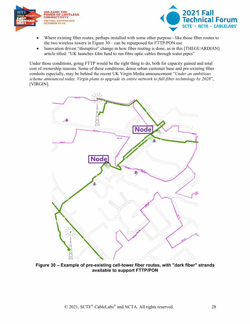
• Where existing fiber routes, perhaps installed with some other purpose - like those fiber routes to the two wireless towers in Figure 30 – can be repurposed for FTTP/PON use

• Innovation driven “disruptive” change in how fiber routing is done, as in this [THEGUARDIAN] article titled: “UK launches £4m fund to run fibre optic cables through water pipes”

Under those conditions, going FTTP would be the right thing to do, both for capacity gained and total cost of ownership reasons. Some of these conditions, dense urban customer base and pre-existing fiber conduits especially, may be behind the recent UK Virgin Media announcement “Under an ambitious scheme announced today, Virgin plans to upgrade its entire network to full-fiber technology by 2028”, [VIRGIN].

Figure 30 – Example of pre-existing cell-tower fiber routes, with "dark fiber" strands

available to support FTTP/PON


4.11. Greenfield scenarios – business as usual or FTTP/PON?

Furthermore, what to build in the green field is the question to revisit often and to revisit hard. Based on our analysis, CAPEX for new builds HFC vs FTTP way - are on par – provided legacy video issues and back-office compatibility are taken out of the discussion. It comes down to the operations folks deciding to continue business as usual or to remove all the obstacles for going the “brave new world” way, and to start doing fiber all the way for all the new / greenfield builds

5. Discussion – The Steps to Get There

5.1. The name of the game is optionality As many Operators contemplate the jump to FTTP, DOCSIS4.0 continues to offer an extremely viable and cost-effective upgrade path, comfortably enabling multi-gigabit services, including symmetric gigabit services for business and enterprises. To maximize their optionality in the coming years, operators are beginning to seed new Extended Spectrum DOCSIS (ESD) passive components in their networks as part of their regular preventive network maintenance (PNM) programs. These new passives are emerging with 1.8GHz rated faceplates and housing supporting 2GHz+, and will enable operators to expand their plant’s spectrum as required; and as they evolve from centralized CCAP platforms; which today are limited to 1.2GHz operation, to distributed access technologies like Remote MACPHY which are evolving to support ESD operation to 1.8GHz. The deployment of distributed access architectures will drive fiber deeper into HFC footprints and strengthen the future economics behind fiber to the home and business. This non-regret investment in their footprints will also provide operators with powerful optionality that allows them to choose the right technology for the right place at the right time.

Operators have many options to choose from as they upgrade their networks to support the bandwidth demands of the future. Their choices will likely be different depending on their particular constraints, challenges and expected Return-on-Investment (ROI). In addition, they may opt to utilize one option for some period of time, and then switch to a different option at a later point in time. Some operators may even choose two or more options to utilize in different markets at the same time.

Faced with the potentially expensive decision of deploying FTTP, one approach to making a sound decision may include an economic cutoff analysis where the level of investment required for FTTP overbuild deployment in a HFC node serving area is compared against the uplift in revenue expected from that investment of fiber coupled with the OPEX savings from not having to maintain an HFC plant; which can be subject to variation by different area’s depending on the geographic and environmental factors (e.g. is the plant overhead or underground? Is it in or adjacent to a coastal location? Is it a high traffic area prone to damage?). This investment analysis should be performed over the expected life of any uplift in HFC plant, which is typically 10-15 years.

Below is a list of potential options, divided into several different constraint types.

o Near-term and Long-term Greenfield Deployment Areas In these areas, operators may opt to roll out FTTP. This is the logical choice, as it provides

long-term bandwidth capacities for the deep future. Since connections must be pulled to each


home anyway, it makes the most sense to utilize the technology with the longest lifespan ahead of it (FTTP).

o Near-term Non-Greenfield Deployment Areas with D3.1-capable HFC plants already in place with

needs for ~3 Gbps (or less) Downstream SLAs and ~1 Gbps (or less) Upstream SLAs In these areas, operators may decide to utilize combinations of several near-term D3.1-

enabled techniques to augment both SLA capacity and per-subscriber average capacity to extend plant life. These techniques can include: • Traditional Node-splits that move towards N+3 or N+2 cascade depths (which can

especially help give more per-subscriber average Upstream Capacity which may be required in the future due to COVID bandwidth demand increases)

• Moving the Upstream split from 42 (or 65) MHz up to 85 MHz or 204 MHz (high-split) • Moving the top-end Downstream frequency from 750 (or 860) MHz to 1.2 GHz (Note:

Getting to 1.2 GHz Downstream/204 MHz Upstream is a valuable interim step, as it will yield:

o ~1.1-1.3 Gbps of Upstream Capacity (supporting ~1 Gbps Upstream DOCSIS SLAs)

o ~5.5-7.5 Gbps of Downstream Capacity (maybe limited to ~2-3 Gbps DS DOCSIS SLAs due to some of the capacity being used by Legacy QAM Video))

In these areas, operations can use combinations of several approaches to reduce the spectrum required to support video, including:

• Using Switched Digital Video (SDV) to reduce spectrum that must be dedicated to Legacy QAM Video

• Moving to IP Video (which offers some of the same benefits of SDV with the transmission of only requested video streams).

• Use more efficient video coding schemes to reduce spectrum that must be dedicated to video

In these areas, operators may use “Selective Subscriber Migration” to move selected subscribers from the HFC network to a parallel FTTP network that only needs to be installed with adequate infrastructure to support the small subset of subscribers selected for this treatment. These selected subscribers will tend to be those who select the highest SLAs and/or those who consume inordinately large amounts of average Bandwidth Capacity. This approach will extend the lifespan of the HFC network for the majority of “normally-operating” subscribers.

o Long-term Non-Greenfield Deployment Areas with D3.1-capable HFC plants already in place with

needs for ~4 Gbps (or greater) Downstream SLAs and/or ~2 Gbps (or greater) Upstream SLAs. • Several approaches are permissible, depending on the constraints and challenges facing

the MSO.

Approach #1 (HFC Focus): • Operators can begin by deploying 1.8 GHz-capable taps (in 3 GHz housings) to seed

the network. This may be a lengthy activity to ubiquitously cover a majority of HFC plants, so it may need to be started many years before the actual 1.8 GHz service is to be enabled. Prior to D4.0 enablement, these taps can be used to transport traditional D3.1 bandwidth capacities peaking at 1.2 GHz Downstream frequencies and 204 MHz Upstream frequencies.

• Alternatively, MSOs can begin deploying 1.6 GHz-capable faceplates in existing tap housings to seed the network. This reduces the maximum Bandwidth Capacity by a


small amount, but it could reduce costs and reduce installment times. Prior to D4.0 enablement, these taps can be used to transport traditional D3.1 bandwidth capacities peaking at 1.2 GHz Downstream frequencies and 204 MHz Upstream frequencies.

• At the same time (or slightly later), MSOs can begin deploying D4.0 1.8 GHz-capable/Ultra-High-Split-capable amplifiers (in 3 GHz housings or in existing housings that can support 1.8 GHz operation) to seed the network. This may be a lengthy activity to ubiquitously cover a majority of HFC plants, so it may need to be started years before the actual 1.8 GHz service or Ultra-High-Split service is to be enabled. Prior to D4.0 enablement, these amplifiers can be used to transport traditional D3.1 bandwidth capacities peaking at 1.2 GHz Downstream frequencies and 204 MHz Upstream frequencies.

• At the same time (or slightly later), MSOs can begin deploying D4,0 1.8 GHz-capable/Ultra-High-Split-capable DAA Nodes (in 3 GHz housings or in existing housings that can support 1.8 GHz operation) to seed the network. This may be a lengthy activity to ubiquitously cover a majority of HFC plants, so it may need to be started years before the actual 1.8 GHz service or Ultra-High-Split service is to be enabled. Prior to D4.0 enablement, these DAA Nodes can be used to transport traditional D3.1 bandwidth capacities peaking at 1.2 GHz Downstream frequencies and 204 MHz Upstream frequencies.

• At the same time (or slightly later), MSOs can begin deploying D4.0 1.8 GHz-capable/Ultra-High-Split-capable CM/Gateways into homes to seed the network. This activity can be done in a ubiquitous fashion or can be done in a targeted fashion, targeting the high-end users who are likely to require D4.0 BW capacities in the future. Prior to D4.0 enablement, these CM/Gateways can be used to transport traditional D3.1 bandwidth capacities peaking at 1.2 GHz Downstream frequencies and 204 MHz Upstream frequencies. It is even possible that these D.40 modems can be used on the D3.1 networks to increase the number of bonded OFDM blocks that the CM can feed into a single home.

• Once the D4.0-capable taps and amplifiers and Nodes and requisite CM/Gateways

are deployed within a particular HFC network, the higher capacity 1.8 GHz Downstream operation and Ultra-High-Split Upstream operation (up to 684 MHz) can be enabled whenever subscriber bandwidth demands and SLA requirements demand the higher capacities. The need for higher SLAs is likely to dominate this activity. Higher SLAs could be required to support subscriber demands, but it is more likely and expected that higher SLAs will typically be required to respond to marketing challenges from other competing Broadband operators offering high-bandwidth service (>3 Gbps) in the same geographical area. The time-frames for the development of these marketing challenges (and the time-frames for the enablement of D4.0 bandwidth capacities) will obviously vary from area to area depending on the nature of the competition in each area. Each MSO will need to predict when these challenges will arise to permit them to properly phase and schedule their D4.0 rollout activities with adequate lead time.

• As was the case for near-term HFC plants, MSOs can still use combinations of several approaches to reduce the spectrum required to support video in their long-term HFC plants, including:

o Switched Digital Video or a move to IP Video (which offers some of the same benefits of SDV) to reduce spectrum that must be dedicated to Legacy QAM Video


o Use more efficient video coding schemes to reduce spectrum that must be dedicated to video

• As was the case for near-term HFC plants, MSOs can still use “Selective Subscriber Migration” to move selected subscribers from the HFC network to a parallel FTTP network that only needs to be installed with adequate infrastructure to support the small subset of subscribers selected for this treatment. These selected subscribers will tend to be those who select the highest SLAs and/or those who consume inordinately large amounts of average Bandwidth Capacity. This approach will extend the life-span of the HFC network for the majority of “normally-operating” subscribers.

Approach #2 (FTTP Focus)

o Operators can begin by targeting high-density subscriber areas (ex: MDUs, high-rises, some city dwellings) for 10G-capable FTTP deployments where the business case analysis indicates there is value. (Note: The business case analysis should be focused on subscriber density, fiber-pull complexity, cost of labor, and whether opportunities exist to share costs of fiber-pulls with other initiatives such as fiber deployments to support cell-tower installations). This FTTP network can initially be built as an overlay to the already-existing HFC network.

o Operators can extend the above FTTP deployment activities to all other areas, extending the 10G-capable FTTP connectivity to all subscribers in high-density subscriber areas, medium-density subscriber areas, and low-density (rural) subscriber areas. This FTTP network can initially be built as an overlay to the already-existing HFC network.

o Operators can begin deploying PON ONT Gateways into homes to seed the network. This activity can be done in a ubiquitous fashion or can be done in a targeted fashion, targeting the high-end users who are likely to require higher BW capacities in the future. Since having both PON and DOCSIS CPE equipment co-existing within a home is probably undesirable to subscribers, the FTTP system must be enabled and operational the moment that the first subscriber in the area receives their PON ONT Gateway equipment. It should be clear that during the transition from HFC to FTTP, the two networks will both be operational and running in parallel. A subset of subscribers will be connected to the HFC network, and a subset of subscribers will be connected to the FTTP network. Over time, more and more subscribers will be moved from the HFC network onto the FTTP network.

Approach #3 (Blended HFC/FTTP Focus)

o This approach permits the MSO to use both Approach #1 and Approach #2. Each of their subscriber areas can be upgraded using a different approach depending on the particular constraints and challenges in that particular area. Business case analyses will need to be done to determine which approach is most suitable for any particular area.

6. Conclusions This paper has studied many different evolutionary paths that MSOs can choose to utilize as they evolve their networks to the higher bandwidth capacities needed for future 10G operations. Each operator will clearly choose the path that yields the best return on investment for their own situation, and each operator


will undoubtedly find themselves with different sets of constraints and challenges as they select their future paths.

In general, this study tended to show that for markets where HFC networks already exist, operators will likely want to augment their existing HFC infrastructure to provide the types of bandwidth capacities that are anticipated to compete in the late 2020’s and 2030’s. Several phases of upgrades are likely. Operators may find a very good return on their existing investment by utilizing DCOSIS 3.1 technologies and traditional node-splitting activities for as long as permissible. This should carry them a long way into the 2020 decade. But to support the bandwidths of the late 2020’s and 2030’s, operators will likely need to begin seeding DOCSIS 4.0 technologies coupled to DAA architectures into their existing HFC networks, perhaps operating the equipment in a DOCSIS 3.1 fashion for a while before enabling the DOCSIS 4.0 operations. This permits the MSOs to seed the DOCSIS 4.0 equipment over multiple years before having to enable it, which is required since it does require changes to many network elements (Nodes, Amps, Taps, and CPEs). Each DOCSIS 4.0 technology has its own strengths and weaknesses. FDX requires less work on taps (although taps will still likely need to be upgraded to 1.2 GHz operation) at the expense of an N+0 plant. ESD operation may be simpler to diagnose (since it uses familiar FDD technologies) and it may yield higher downstream throughput capacities when N+2 plants are permitted. ESD may also provide cost benefits over FDX.

For Greenfield markets, the study showed that it is beneficial to consider FTTX as a starting point, because the higher cost of initial deployment is a given, and the FTTX technology provides larger bandwidth capacities for the long-term.

In either case, it is clear that MSOs have many good options from which to choose as they augment their networks to support the 10G services of the future.


Abbreviations

10G 10 gigabits per second 5G 5th generation mobile network AR augmented reality BW bandwidth CAGR compound annual growth rate CAPEX capital expenditures CM cable modem CMTS cable modem termination system COVID corona virus disease CPE consumer premise equipment D3.1 DOCSIS 3.1 D4.0 DOCSIS 4.0 DAA distributed access architecture DFN distribution fiber network DOCSIS data over cable service interface specification DS downstream ESD extended spectrum DOCSIS FDX full duplex FTTN fiber to the node FTTP fiber to the premise FTTT fiber to the tap FTTX fiber to the “X” GIGO “garbage in, garbage out” HEO head-end optics HFC hybrid fiber coaxial HP homes-passed I-CCAP integrated converged cable access platform IG interference group IP internet protocol IPTV internet protocol television KISS keep it sophisticatedly simple; or, keep it simple and straightforward MAC media access control Mbps megabits per second MDU multi dwelling unit MSO multiple system operator NPV net present value OFDM orthogonal frequency division multiplexing OFDMA orthogonal frequency division multiple access OLT optical line terminal ONT optical network terminal ONU optical network unit OPEX operating expenditures PHY physical layer PNM proactive network maintenance PON passive optical network


QoE quality of experience RF radio frequency ROI return on investment SC-QAM single carrier quadrature amplitude modulation SDV switched digital video SFP small form factor pluggable SG service group SLA service level agreement TCO total cost of ownership US upstream VR virtual reality

Bibliography & References [CLO_2013] T. J. Cloonan et. al., “Advanced Quality of Experience Monitoring Techniques for a New Generation of Traffic Types Carried by DOCSIS,” NCTA Spring Technical Forum 2013, NCTA

[CLO_2014] T. J. Cloonan et. al., “Simulating the Impact of QoE on Per-Service Group HSD Bandwidth Capacity Requirements,” SCTE Cable-Tec 2014, SCTE

[EMM_2014] “Nielson’s Law vs. Nielson TV Viewership for Network Capacity Planning,” Mike Emmendorfer, Tom Cloonan; The NCTA Cable Show Spring Technical Forum, April, 2014

[VENK_SCTE_2016] “Cable’s Success is in its DNA: Designing Next Generation Fiber Deep Networks with Distributed Node Architecture” Venk Mutalik, Zoran Maricevic; 2016 SCTE Cable-Tec Expo

[AYHAM_SCTE_2019] “Operational Considerations & Configurations for FDX & Soft-FDX - A Network Migration Guide To Converge The Cable Industry” Ayham Al-Banna, Frank O’Keefe and Tom Cloonan; 2019 SCTE Cable-Tec

[ULM_2019] J. Ulm, T. J. Cloonan, “The Broadband Network Evolution continues – How do we get to Cable 10G?”, SCTE Cable-Tec Expo 2019, SCTE

[ULM_2020] J. Ulm, Z. Maricevic, F. O’Keefe, “Is “Unity Gain” Still the #1 Objective? – Maybe YES!”, SCTE Cable-Tec Expo 2020, SCTE

[ULM_2021] J. Ulm, M. Zimmerman, S. Eastman, Z. Maricevic, “Overlaying Mid-Band Spectrum Backhaul/Fronthaul onto HFC – A Symbiotic Convergence of Cable & Wireless”, SCTE Cable-Tec Expo 2021, SCTE

[SATELLITE] Satellite Internet Access, https://en.wikipedia.org/wiki/Satellite_Internet_access

[FORBES] How Fast Will 5G Really Be?, https://www.forbes.com/sites/bobodonnell/2019/11/19/how-fast-will-5g-really-be/?sh=199eb2cc5cf3

[ITU] ITU-T PON Standards: Progress and Recent Activities, https://www.itu.int/en/ITU-T/studygroups/2017-2020/15/Documents/OFC2018-2-Q2_v5.pdf

https://en.wikipedia.org/wiki/Satellite_Internet_access

https://www.forbes.com/sites/bobodonnell/2019/11/19/how-fast-will-5g-really-be/?sh=199eb2cc5cf3

https://www.forbes.com/sites/bobodonnell/2019/11/19/how-fast-will-5g-really-be/?sh=199eb2cc5cf3

https://www.itu.int/en/ITU-T/studygroups/2017-2020/15/Documents/OFC2018-2-Q2_v5.pdf

https://www.itu.int/en/ITU-T/studygroups/2017-2020/15/Documents/OFC2018-2-Q2_v5.pdf


[VIRGIN] “Virgin dooms DOCSIS in UK with fiber-for-all plan”, 7/29/2021, https://www.lightreading.com/opticalip/fttx/virgin-dooms-docsis-in-uk-with-fiber-for-all-plan/d/d-id/771160?

[THEGUARDIAN] “UK launches £4m fund to run fibre optic cables through water pipes”, 08/08/2021, https://www.theguardian.com/technology/2021/aug/09/uk-launches-4m-fund-to-run-fibre-optic-cables-through-water-pipes

https://www.lightreading.com/opticalip/fttx/virgin-dooms-docsis-in-uk-with-fiber-for-all-plan/d/d-id/771160

https://www.lightreading.com/opticalip/fttx/virgin-dooms-docsis-in-uk-with-fiber-for-all-plan/d/d-id/771160

https://www.theguardian.com/technology/2021/aug/09/uk-launches-4m-fund-to-run-fibre-optic-cables-through-water-pipes

https://www.theguardian.com/technology/2021/aug/09/uk-launches-4m-fund-to-run-fibre-optic-cables-through-water-pipes

DOCSIS 4.0 - A Key Ingredient of the 2030's Broadband Pie

Documents

Transcript of DOCSIS 4.0 - A Key Ingredient of the 2030's Broadband Pie