MANAGERIAL ECONOMICS

AHSAN KABIRAHSAN KABIR1 M

ANAG

ERIA

L EC

ONOM

ICS

For s

tude

nts

of E

CONO

MIC

S ,B

BA a

nd M

BA

MANAGERIAL ECONOMICS Chapter One:

Introduction to Economics

Economics, social science concerned with the production, distribution, exchange, and consumption of goods and services. Economists focus on the way in which individuals, groups, business enterprises, and governments seek to achieve efficiently any economic objective they select. Other fields of study also contribute to this knowledge: Psychology and ethics try to explain how objectives are formed; history records changes in human objectives; sociology interprets human behavior in social contexts.Standard economics can be divided into two major fields. The first, price theory or microeconomics, explains how the interplay of supply and demand in competitive markets creates a multitude of individual prices, wage rates, profit margins, and rental changes. Microeconomics assumes that people behave rationally. Consumers try to spend their income in ways that give them as much pleasure as possible. As economists say, they maximize utility. For their part, entrepreneurs (see Entrepreneur) seek as much profit as they can extract from their operations.

The second field, macroeconomics, deals with modern explanations of national income and employment. Macroeconomics dates from the book, The General

AHSAN KABIR2

MANAGERIAL ECONOMICSTheory of Employment, Interest, and Money (1935), by the British economist John Maynard Keynes. His explanation of prosperity and depression centers on the total or aggregate demand for goods and services by consumers, business investors, and governments. Because, according to Keynes, inadequate aggregate demand increases unemployment, the indicated cure is either more investment by businesses or more spending and consequently larger budget deficits by government.

The story begins: Scarcity and choiceIn this world, our desires are unlimited. Our ability to meet these desires are, however, limited. This concept is popularly known as scarcity. Although this may seem to be self-evident truth, it gives birth to a great insight that the story starts with. Because, as we face the problem of scarcity, we know that we can’t have all the goods and services, which we desire. We have to choose few among many desired goods that we afford to have. It gives rise to the problem of choice: what to choose and what to miss?

This is a problem and the implication of it is clear. Suppose, I want both a TV and a computer, but can afford to buy only either TV or Computer. Now, if I go for a TV, certainly I’ll miss out the opportunity of availing a computer, and vice versa. So, as we call it in

AHSAN KABIR3

MANAGERIAL ECONOMICSeconomics, the opportunity cost of getting the TV is the computer that I could not have because of scarcity of resources.

What is economics all about?

Now, we tell you in few words, what “economics” talks about. Economics is the scientific study of possible alternatives to use our limited resources in such efficient way that we ensure the highest level of satisfaction or welfare.

Normative vs. Positive economics

A word of caution is warranted here. Like all other science discipline, in the present day economics, we never discuss how we should maximize our welfare. We can only talk about how people are actually making it. Economics is silent to the question: what should be done? It is rather talkative about to answer what is actually done. Economics is positive that is value-neutral study of the reality, not normative that involves ethical precepts and norms of fairness in approach.

Basic problems of economic organization

Every human society must confront and resolve three fundamental economic problems. Every society must have a way of determining

AHSAN KABIR4

MANAGERIAL ECONOMICS1) what commodities are produced (i.e. allocation of limited resources),

2) how these goods are made (i.e. production methods) and

3) for whom they are produced (i.e. distribution mechanism).

What are the different ways that a society can answer these questions of what, how and for whom? Different societies are organized through alternative systems.

We generally distinguish two fundamentally different ways of organizing an economy. On one hand, a Market Economy is one in which al these three questions are answered through the market. In this extreme case, the government does not interfere in the market and it is called laissez –faire economy.

In contrast, a command economy is one in which the government makes all important decisions about production and distribution through its ownership of resources and its power to enforce decisions.

No contemporary society however falls completely into either of these polar categories. Rather all societies are mixed economies, with elements of market and command economies.

AHSAN KABIR5

MANAGERIAL ECONOMICSOpportunity Cost and Production Possibility Frontier

In order to understand how the concept of opportunity cost relates to the real world situations, we may use the concept of the production possibility frontier. A production possibility frontier shows different choices or possible combinations of two goods that can be produced by a nation using all of its resources i.e. land, labor and capital. The following numerical table lists some choices of the nation that can produce, say, foods and cloths using all of its resources.

Choice Foods(thousand tons) Cloth (thousand units)

A 0 50

B 1 42

C 2 30

D 3 16

E 4 0

The following diagram plots what we have in the table. Suppose, along the vertical axis we measure quantity of cloth produced and along the horizontal axis quantity of Foods produced. Suppose the economy is producing at choice B, i.e. 1,000 tons of foods and 42,000 units of

AHSAN KABIR6

MANAGERIAL ECONOMICScloth. Now if it wants to produce one more thousand

tons of foods, it can do it only by reducing the production of cloth from 42,000 to 30,000 thousand units of cloth. Therefore, we can say that the opportunity cost of getting one extra thousand tons of foods is 12,000 thousand units of cloth that we have lost. It happens because the total amount of resources is limited for a nation. If we want more of an opportunity, we have to make a sacrifice to lose part or whole of another opportunity. This is true at very personal as well as national level.

Market and Market EconomyThe economic system in which all basic problems of what, how and for whom are answered through market is called a market economy.A market is a mechanism by which buyers and sellers interact to determine the price and quantity of a goods or service. In a market system, everything has a price, which is the value of the good in terms of money.

AHSAN KABIR7

MANAGERIAL ECONOMICSIn addition, prices serve as signals to producers and consumers. If consumers want more of any good, the price will rise, sending a signal to producers that more supply is needed. On the other hand, if a commodity is overstocked, price of it will be lowered to clear the stock. At lower price, consumers will buy more, but producers will be unwilling to produce much of that commodity. As a result, a balance, or equilibrium, between buyers and sellers will be restored. Market equilibrium represents a balance among all the different buyers and sellers.

The two major failures of a market economy are inefficiency that arises out of monopoly and externalities, and unacceptable inequalities of income and wealth among people.What is managerial economics?The global economy presents managers with many more opportunities and many more choices than they have had in the past. These choices are not limited to the question of where to sell ones product. For example, to be an efficient producer, a firm must now, more than ever, determine where to obtain both its inputs (labor, equipment, parts and materials, etc.) and its technology. This is not just a case of substituting cheap foreign labor for expensive domestic labour (in case of USA, for example) or substituting expensive foreign labor for cheap domestic labour (in case of Bangladesh,

AHSAN KABIR8

MANAGERIAL ECONOMICSfor example). It has to do with other considerations, such as the quality of labour for specific technical tasks and the type of technology best suited to a firm’s product line. While the United States, Japan, and Western Europe are technological giants, cutting-edge technologies have been developed and are available from such places as Mexico (e.g. directly reduced iron) and Russia (e.g. laser surgery equipment, rocket technology etc.). Managerial economics focuses on the types of choices described above. Its central themes are:

1. Identifying problems and opportunities; 2. Analyzing alternatives from which choices can be made; and3. Making choices that are best (optimal) from the standpoint of the firm or organization.Because managers are always confronted with situations involving choosing from among alternative policies or strategies (whether to go into a new product line, whether or not to employ a new technology, whether to consider production in a foreign market, and many other types of choices), the tools of managerial economics are important to them. It is certainly not true that all managers must also be managerial economists. However, managers who understand the way managerial economics applies basic economic analysis to the specific problems encountered by firms and other

AHSAN KABIR9

MANAGERIAL ECONOMICSorganizations are more likely to choose wisely than those who do not. This becomes increasingly the case as developments on the international scene broaden both our opportunities and our range of choices. Role of Managerial Economics in Problem Solving Whether one's major field is accounting, marketing, information systems, finance, or some other specialization, the analytical abilities that are sharpened by a familiarity with applied economics are extremely valuable. Take, for example, the issue of pricing. Suppose you are considering whether or not to reduce the price of a given product. What is the most fundamental question one can ask in this regard? It has to be "will sales revenue increase or decrease as a result of this change in price?" Managerial economics can help to answer that question, and in a business, someone who has skills similar to those of a managerial economist will be able to answer it, given the appropriate data. Managerial economics not only looks at problems in pricing, but also in such areas as production, input use, cost, profit, and investment decisions. The tools and techniques it offers in analyzing these questions carry over into many others. They help people to communicate their own thoughts as well as to understand what others in a firm or organization are trying to tell them.

AHSAN KABIR10

MANAGERIAL ECONOMICSThe desired output of both research and managerial activities in a firm or organization is a set of decisions that are best for it, given its environment and the resources it has to work with. These are called optimizing decisions. Macroeconomics, Microeconomics, and the Corporate EconomistEconomists generally divide their discipline into two branches, macroeconomics and microeconomics. Macroeconomics focuses on the study of the economy as a whole and deals with issues such as the level of overall activity (gross domestic product or GDP), interest rtes, federal budgets, international trade and currency questions, and federal taxes. Microeconomics, on the other hand, deals with the behavior of individual economic units, such as a consumer or a business firm. In this book we deal primarily with microeconomics, since we are addressing how economic analysis can be used to make decisions within a firm or organization. Nonetheless, corporate economists are frequently asked to prepare research reports and suggest strategies relating to both macro and microeconomic. There are many firms and public sector organizations that are not large enough to have their own economists group and must either rely on consultants or in-house staff with some economics training to apply economic principles to decision problems. Generally, managers in these firms and organizations are interested in

AHSAN KABIR11

MANAGERIAL ECONOMICSeconomic analysis only to the extent that it has something to say about questions that influence performance or profits. Thus, they are even more likely to ask questions of a microeconomic nature than are certain managers of larger corporations or organization. Managers and Their ObjectivesThe managers of a firm are responsible for making most of the economic decisions - the type of product produced, its price, the production technology used, and the financing of production - that will ultimately result in profits or losses for the firm. The firm's manager or managers may or may not be its owner; therefore the goals of the managers may not be quite the same as those of the owner. There may be an incentive for the managers to act in ways that are not in the best interests of the shareholders. Economists call this type of problem a principle-agent problem. The recent debate over managerial compensation is related to various hypotheses about the nature of business firms. The most widely employed hypothesis in managerial economics is that firms will be operated in a way that leads to profit maximization. While this seems to be a reasonable hypothesis, the principal- agent problem suggests that it is open to question. Economists and specialists in organizational management have derived other hypotheses about the behavior of firms and have done a great deal of

AHSAN KABIR12

MANAGERIAL ECONOMICSresearch aimed at testing these hypotheses. The following are some of the alternative hypotheses.

1. Market share maximization. Firms will behave in a way that maximizes market share (as measured by sales revenue, or perhaps, proportion of quantity sold to total market).

2. Growth maximization. Increasing the size of the firm over time will take precedence over other objectives. Profit may be sacrificed to attain higher rates of growth in other variables.

3. Maximization of managerial returns. Managers will make choices that maximize their own interest, subject to generating sufficient profit to keep their jobs.

The results of empirical testing of these hypotheses, as well as tests of the profit-maximization hypothesis, have been mixed. At different points in time and under different states of the economy (expansion or recession) one or the other seems to have empirical support. However, economists generally favored the profit maximization hypothesis for a variety of reasons. First and foremost, a firm that is not profitable is unlikely to survive in the long run. Second, while managerial rewards may be at some points in time and in some firms more closely correlated with sales or growth than with profit, as we have seen, shareholders and

AHSAN KABIR13

MANAGERIAL ECONOMICSgovernment regulators alike are interested in designing compensation packages that are tied to profit performance. Third, profit maximization requires careful study of factors, like demand and cost which will remain important even when the firm has another main objective or a set of more complex objectives. Finally, if one does not know what results a profit-maximizing strategy will yield; it is not possible for him to assess the cost to the firm of pursuing alternatives to it. For all of these reasons, in this course we will generally assume that the objective of a firm is profit maximization. Questions for discussions

1. What is scarcity? Explain how does it lead to the problem of choice?

2. What are the basic economic problems of a society?

3. Explain the concept of opportunity cost.4. What is the central theme of managerial

economics?5. What are the alternative objectives of a firm?

Why profit maximization is the most chosen firm objective in economics?

AHSAN KABIR14

MANAGERIAL ECONOMICS

Chapter Two: Basic Elements of Supply and

Demand

Markets are akin to weather. They are always changing, dynamic, unpredictable, complex, and fascinating. Economics has developed a very powerful tool for explaining these, and many other changes in the economic environment. It is called the theory of supply and demand.

The Law of DemandThe law of demand states that buyers of a good will purchase more of the good if its price is lower (and vice versa). If the price of strawberries decreases from $2.00

AHSAN KABIR15

MANAGERIAL ECONOMICSper pound to $1.00 per pound, consumers will buy more strawberries.

The law of demand holds, as economists say, “ceterus paribus”, or: “assuming other relevant variables remain constant.” It would be possible, for example, that as the price of strawberries decreases from $2.00 per pound to $1.00 per pound, fewer pounds of strawberries are purchased.

One reason may be that buyers’ real incomes decline, so that, even though the price of strawberries is lower, they just can’t afford to buy as many. Does this then violate the law of demand? The answer is “no”, because the latter example is an instance where another relevant variable was not held constant. If all relevant variables had remained constant, then we would have seen an increase in the purchase of strawberries as a result of a price decrease.The Demand CurveDemand data can be graphed in a diagram. The two variables to consider are the price of the product and the amount of the product purchased during a certain period of time. Economists usually measure the price of the good on the vertical axis and the quantity on the horizontal one.In the diagram below, two points are plotted for a particular product (for example, watching an ice hockey

AHSAN KABIR16

MANAGERIAL ECONOMICSgame at the US Air Arena). At ticket prices of $7.00, 13 (thousand) tickets are sold.And at $14.00 per ticket, only 6 (thousand) seats are sold. Other points can be plotted and a line or curve can be connected through these points to come up with this good’s demand curve. Individual product demand curves always extend from the upper left to the lower right, i.e., they are downward sloping.

The above diagram shows that on demand curve D consumers buy 13 units at a price of $7 (point A) and 6 units at a price of $14 (point B). The Law of SupplyThe law of supply states that product suppliers (firms) offer more of a product at higher than at lower prices (just the opposite of the law of demand). If the product price is high, the firm can make greater profits by selling more (assuming the cost of production is

AHSAN KABIR17

MANAGERIAL ECONOMICSconstant and the demand for the product is there). A video game, for which the demand is high and therefore the price as well, will be supplied at greater quantities because the higher price makes firms want to supply more.

The Supply CurveA supply curve is upward sloping from the bottom left of the graph to the upper right of the graph. This indicates that at higher prices firms supply more than at lower prices and there is a direct relationship between price and quantity supplied.

The above diagram shows that on supply curve S firms supply 6 units of this product when the price is $7 (point A) and 11 units when the price is $14 (point B).Equilibrium Price and Quantity

AHSAN KABIR18

MANAGERIAL ECONOMICSIn a free market (competitive and with no government involvement) the equilibrium price and quantity occur where the supply and demand curves intersect. At this price consumers are willing to buy the same amount which businesses are willing to offer. If the price were below this intersection point, a shortage would exist. If the price were above equilibrium, we would experience a surplus.

In the graph above, this market is at equilibrium at a price of $11 and a quantity of 9. When the price is set at $7, a shortage of 7 products (13 minus 6) will result. If the price were $14, there would be a surplus of 5 units (11 minus 6).Demand Determinants

AHSAN KABIR19

MANAGERIAL ECONOMICSThe demand schedule (curve) does not always stay in the same position. The following are reasons why it may change, i.e., why demand increases or decreases:A. A change in buyers’ incomes and wealth.The demand for most products will go up if buyers’ real incomes or real wealth, i.e., their purchasing power, rise. For example, if I manage to earn $50,000 next year instead of $40,000 this year (and assuming that there is no increase in the price level so that my real income increases), I will find myself purchasing more clothes, restaurant meals, etc.Consequently, the demand for these products increases.Notice that some products or categories of products may experience a decline in demand as a result of my higher income, because my higher income allows me to purchase more expensive (“normal”) substitute products. Typical examples of these so-called “inferior” goods are potatoes, public transportation, spaghetti meals, generic products, etc.B. Buyers’ tastes and preferences.Because something is in fashion, the demand for the product may increase. Example: home videos, fat free mayonnaise and ice cream, online products, and virtual reality games.C. The prices of related products or services.Consider the market for potato chips. The demand for it will go down (assuming no other changes) if the price of a related good, for example, pretzels, decreases. So, if

AHSAN KABIR20

MANAGERIAL ECONOMICSthe price of a substitute falls, then the demand for the product in question drops (and vice verse). A related good can also be a complement. This is a product consumed not in place of, but along with another good. A drop in the price of potato chips dip is expected to increase the demand for potato chips. So if the price of a complement falls, the demand for the other product rises (and vice versa).D. Buyers’ expectation of the product’s future price.When a supermarket announces that potato chips will become more expensive in the near future, more people will tend to buy the product now (and vice versa). This would increase current demand and shift our demand curve to the right. Notice that this will have the eventual effect of raising the real price and thus fulfilling the expectation.E. The number of buyers (population).If the population of buyers of a certain product increases, we will experience an increase in the demand for that product. With the aging of the baby boomers we can anticipate a rise in the demand for products which senior citizens typically purchase (insurance, health care, travel, nursing care).Demand versus Quantity DemandedEconomists distinguish between a change in demand and a change in quantity demanded. These terms may sound similar but they are different in “econobabble.”

AHSAN KABIR21

MANAGERIAL ECONOMICSDemand increases (or decreases) when the demand curve shifts. This occurs because of the demand determinants (as described in the previous paragraph) changed.

Quantity demanded increase (or decreases) because the price of the product changed. This can be illustrated by a movement along (not a shift in) the demand curve.Consider the market for ice cream. If people decide to consume more ice cream because their incomes go up, we speak of an increase in the demand for ice cream. If consumers purchase more ice cream because the price is lower (because the supply has gone up), we call this an increase in quantity demanded.

In the above graph demand increases as D1 shifts to D2. As a result, quantity supplied increases and the equilibrium point shifts along the supply curve from point A to point B.

AHSAN KABIR22

MANAGERIAL ECONOMICS

The Effect of a Change in Demand on Equilibrium Price and Quantity

When the demand curve shifts to the right, i.e., demand increases, then the market price will go up, as will the equilibrium quantity (in the short run).

AHSAN KABIR23

MANAGERIAL ECONOMICSWhen the demand curve shifts to the left, both price and quantity will decline (in the short run).

Supply DeterminantsFour reasons why firms may supply more of a product are:A. Advance in technology.An advance in the technology of making the product will lower the cost of producing it. This means that firms will want to supply more of the product.B. Prices of inputs necessary to make the product.When input prices (of labor, raw materials, etc.) go down, the firm can make more profit per product and will want to increase the supply of the product (and vice versa).C. Taxes and subsidies.Taxing the manufacturing of a product will lower the supply (it costs more to make it), and a subsidy does just the opposite.D. The number of firms selling the product.When more firms decide to enter the market the supply of the product increases, and vice versa.Note that any of the above changes will bring about a shift in the supply curve.

Distinguish between a change in quantity supplied and a change in supply

AHSAN KABIR24

MANAGERIAL ECONOMICSThe distinction between supply and quantity supplied is analogous to the difference between demand and quantity demanded. Can you describe this distinction?

The above diagram illustrates that supply increases as S1 shifts to S2 and quantity demanded increases as the equilibrium point shifts along the demand curve from point C to point D.

The Effect of a Change in Supply on Equilibrium Price and Quantity

AHSAN KABIR25

MANAGERIAL ECONOMICS

An increase in supply is illustrated by a rightward (or downward) shift of the supply curve. This will lower the price and increase the output sold in the market.

AHSAN KABIR26

MANAGERIAL ECONOMICSConversely, a decrease in supply (a leftward or upward shift) will raise the price and lower the equilibrium quantity.

Determine how changes in the demand and supply curves affect equilibrium price and quantity.

Let’s analyze the following examples.

Suppose that you know that consumers’ incomes have gone up, and that an advance in technology has lowered the cost of making computers. Assuming that a computer is a normal good, what will happen to the price and quantity of computers as a result of the above two changes?

AHSAN KABIR27

MANAGERIAL ECONOMICSAnswer: An increase in consumers’ incomes will increase the demand of computers (D shifts to the right). Consequently, the quantity will rise and price will either rise, fall, or stay the same, depending on the size of the shifts in the curves (i.e., price is indeterminate). (This is illustrated above.)

Buyers expect videotapes to be higher; and at the same time the government decides to tax the production of videotapes (in an attempt to reduce the budget deficit). What effect does this have on the market price and output of videotapes?

Answer: Demand increases and supply decreases, therefore the price of videotapes will go up; equilibrium quantity is indeterminate. Note that when both the demand and the supply curve shift, one variable undergoes a definite change, but the other is always indeterminate (unless you know the magnitude of the shifts). When only one curve shifts, both the price and amount bought and sold will experience a definite change. This is illustrated in the next graph.)

AHSAN KABIR28

MANAGERIAL ECONOMICS

Determination of Prices in our Economic SystemTheoretically the laws of demand and supply are well established and few economists disagree about the basic nature and the relationships between price and quantity on the demand and the supply side. However, there does appear to be disagreement about the determination of prices of some categories of goods and services. Controversy exists as well about whether the determination of prices should be left solely to supply and demand forces, i.e., the free market, or whether government should have the right to interfere.

Let’s turn to the first question: are prices of all goods and services in a free, laissez-faire market economy determined by supply and demand? Prices of goods that are in limited supply, such as factors of productions (land, labor, etc.), fluctuate much more with changes in demand than goods which are generally abundant (manufactured goods, such as cars, grocery items,

AHSAN KABIR29

MANAGERIAL ECONOMICSclothes, etc.). If, for example, the demand for land in a certain area rises because of increased population and housing activity in this area, one will see the price of the land increase significantly. The price of the land is affected by the demand and is capable of remaining high for a long period of time. The supply cannot increase to bring the price down later, because the factor of production, land, is limited and fixed.

Prices of manufactured goods do not respond to demand and supply forces in this way, at least not in the long run. When the demand for, say, a retail good, such as running shoes, increases, the price increases. A higher price for the makers and suppliers of the shoes means that profits will be higher, assuming that the cost of producing the shoes has remained the same. However, in the long run these profits will not be sustained. Because the profits exceed the average level of profits in most other industries, therefore, other entrepreneurs will want to take advantage of investing in this industry. This increases supply and brings the price back down. The price will go down to a level where profits are normal or average (except in cases where a firm has a monopoly, or a patent, license, etc.). Consequently the price is set such that it covers the cost of producing the good plus a fair allowance for a profit. In the long run then, prices of manufactured goods, i.e., goods that can be produced in practically

AHSAN KABIR30

MANAGERIAL ECONOMICSunlimited quantities (unlike factors of production), are based on the cost (including an allowance for profit) or producing the good.

Advantages and Disadvantages of a Free Market SystemA free market or laissez-faire or pure capitalist economy is one where prices of all goods and services, including wages, interest rates, wages, foreign exchange values, etc., are set by businesses without any interference from government in the form of price controls, labor laws or other regulations. The most important advantage of this is that products are always priced according to their true “worth”, which is based on demand for factors of production, or cost of production for manufactured goods. If a manufactured good costs $10 per item to produce, it will be sold for $10 plus a little extra to allow for a profit. Assuming it is a useful and desired product, consumers will buy it and producers will produce as many products as the demand dictates.

Case One: Let’s say now that the government ordered manufacturers of this product to sell the product for $8. Consumers would have no problem buying the product at this lower price. However, producers, faced with a cost of making the product of $10 dollars, would lose money every time they produced the good and would

AHSAN KABIR31

MANAGERIAL ECONOMICStherefore have no incentive to make the product. Some may produce the product with cheaper ingredients or at a much lesser quality to try to bring the cost down to around $8.; the initial product, produced at a high quality, will not be produced anymore though.

Case Two: If the government ordered the price of the product higher than the market price, say $14, then producers would have no problem selling it for that price as they would experience higher profits per product. However, the higher price would turn away many consumers and they would demand much less of the product than at the old price. Consequently, less of the product will be sold in the market and this constitutes an inefficient allocation of resources.

Concluding remarks: Any time government interferes with the working of the free market, inefficiencies in the market occur in the form of shortages, surpluses, misallocations of resources, mal-investments, business losses, etc. From an economic point of view, this is never desired. The government’s purpose for interfering is to try to remedy certain social problems. In reality it never appears to be successful though. For instance, in the case of rent controls in large cities, the government dictates to many landlords to keep the rent of their apartments, houses, etc. below a certain level. The result of this is that it becomes unprofitable for many

AHSAN KABIR32

MANAGERIAL ECONOMICSlandlords to invest in property or build additional properties to later rent out. Then rent which the government allows them to charge is just not worth their expenses and investment. Consequently, fewer properties will now be available and considerable shortages occur. The lucky few who do manage to obtain a place to rent will pay less than the market price (at least in the short run), but their dwelling will be much less carefully maintained, because the landlord will not be able to afford it. But more importantly, the rent control prevents thousands of unlucky homeless people from acquiring anything because the artificially low rent discourages many potential builders from building additional apartments and houses.

Questions for Discussions

AHSAN KABIR33

MANAGERIAL ECONOMICS1. Briefly explain the law of demand and law of

supply.2. With the help of a diagram, show the equilibrium

price and quantity in a market.3. What are determinants of demand and supply?4. Using a diagram, show how a change in any

determinants of demand changes the market equilibrium.

5. Using a diagram, show how a change in any determinants of supply changes the market equilibrium.

6. With an example, explain how intervention of the government may cause inefficiency in a market.

Mathematical Appendix

Determining Equilibrium Price and Quantity

AHSAN KABIR34

MANAGERIAL ECONOMICSSuppose parameters of the demand and supply equations have been estimated and that the equations are

and

Now, determine the equilibrium price and quantity.

Solution: Note that the slopes of these functions correspond to what we learned earlier, that is, the demand function slopes downward (look at the negative value of the slope or the second term) and the supply curve slopes upward (look at the positive value of the slope or the second term). Setting the demand function equal to the supply function,

Or, Qd = Qs

And solving for the price yields

Substituting into the demand function yields the equilibrium quantity

AHSAN KABIR35

MANAGERIAL ECONOMICS

Thus the [price , quantity] combination results in equilibrium in this market.

Chapter Three: Elasticity and Revenue

Concept of ElasticityNow that we are familiar with the law of demand, we can discuss the concept of elasticity. We know that if the price of strawberries decreases, more will be purchased (ceteris paribus) and vice versa. We don’t know how much though. The elasticity of a product will tell us. Before we elaborate on this, let’s take a look at a few more characteristics of a demand curve.The Derivation of Demand CurvesEconomists who work for large firms might be asked to estimate the demand curve of a product the company is producing. Some ways of doing this are:1. Look at historical data and see how consumers have responded to changes in the price of the product. A potential problem with this might be that many other

AHSAN KABIR36

MANAGERIAL ECONOMICSfactors in the economy have changed, too, so that it is hard to isolate the relationship of only these two variables.2. Experiment with a price change and see how consumers respond.

3. Survey consumers to see how they might respond to a change in the price of the product.This is not always accurate because consumers don’t always know in advance how they will respond to a price change. However, estimates of this demand information will allow us to graph the demand curve and determine its location and slope.In reality it is very difficult to pinpoint the exact location of any demand curve. This is because so many variables related to demand (incomes, technology, the supply curve, etc.) change so frequently and it is difficult to study the relationship between just price and quantity (which is what a demand curve represents), holding everything else constant. Any picture of a demand curve for a particular product therefore, is always an approximation.Price Elasticity of DemandFrom the chapter on supply and demand we already learned that as the price of a product rises, the amount of people buy of it falls. Elasticity measures exactly how much less people buy of that product when the price rises, or vice versa.

AHSAN KABIR37

MANAGERIAL ECONOMICSFor example, if the price elasticity of demand for soap is 3, then when the price of soap goes up by 10% people will buy 30% (3 times 10%) less soap.

Price elasticity of demand is defined as:The percentage change in quantity demanded divided by the percentage change in the price of the product.OR:(change in quantity purchased/average quantity) divided by (the changed in the price/average price).This latter formula is called the “arc” price elasticity of demand. There are other ways to calculate elasticity, but we will restrict ourselves to the formula above.A Numerical ExampleLet’s compute the price elasticity of demand for Mariah Carey concert tickets. Suppose that for one of her concerts the price of a ticket is $15.00 and that 25,000 people attend it. For another, similar concert the organizers charge $17.00 and 24,000 fans show up. What is the price elasticity of demand for tickets in this instance?Answer: Using the formula in the previous objective we get:(1,000/24,500) / (2/16) = .0408/.125 = .3264So the elasticity in this example is about .33 or 33%. This means that if concert tickets increased in price by 100% then 33% fewer people would show up. The true

AHSAN KABIR38

MANAGERIAL ECONOMICSvalue of the above elasticity is -.33 (minus .33). However, because price elasticity of demand is always negative, the minus is assumed and left off.

Determinants of Price Elasticity of DemandWhat makes people more sensitive to one product’s price change than another product’s price change? For example, some people will give up buying a car if its price increases by 10%, but are unaffected by an increase of 50% in the price of a pound of salt.Three determinants of price elasticity of demand are:1. The availability of close substitutes. If a product has many close substitutes, for example a certain brand of cereal, then people tend to react strongly to a price increase, i.e. the price elasticity of this product is high. 2. The importance of the product’s cost in one’s budget. If a product is very inexpensive, such as salt, consumers could care less whether the price of salt goes up by 10, 20, or even 50%. Salt therefore has a very low price elasticity of demand.3. The period of time under consideration. If you’re looking at the demand for gasoline over only one day, people will react less strongly to a price increase than if you studied the effect of a price increase in gasoline over a period of two years. This is because people have much more time to adjust their consumption in two years than in one day.

AHSAN KABIR39

MANAGERIAL ECONOMICSOver the course of two years you have the ability to move closer to work or school; arrange to carpool; buy a more fuel efficient car, etc.

Elasticity, Inelasticity, and Unit ElasticityThere is a simple agreement to distinguish between the above:A product is price elastic when the elasticity is greater than 1. A product is priced inelastic when the elasticity is less than 1. A product is unitary elastic when the elasticity is equal to 1. Note that if elasticity is greater than 1 (elastic), the percentage change in quantity is greater than the percentage change in price (numerator bigger than denominator). For example, if a product’s price rises by 13% and the quantity demanded goes down by more than 13%, then this product is elastic (and vice versa).Elasticity: Another ExampleLet’s look at the three cases: elasticity, inelasticity, and unit elasticity.When a product is elastic, and its price rises, then we expect to see a fall in the sales revenue for that product. To explain this, note that a firm’s total revenue equals Price times Quantity or P x Q. In the above case ,P rises but Q falls. Which one changes more?Answer: Q, because the product is elastic. So the decrease is bigger than the increase and

AHSAN KABIR40

MANAGERIAL ECONOMICSP x Q = TR will fall. For similar reasons: When a product is elastic and its price falls, we will see an increase in TR. When a product is inelastic and its price rises, we will see a rise in TR.

When a product is inelastic and its price falls, we will see a decrease in TR.When a product is unit elastic and its price changes ,we will see no change in TR.

Elasticity and Revenue

One important application of elasticity is to help clarify whether a price increase will raise or lower revenue. This is a key question for many businesses. Total Revenue is by definition equal to price times quantity (or, P x Q). If one knows the price elasticity of demand for his product, he knows what will happen to total revenue when price changes:

1. When demand is price-inelastic, a price decrease reduces total revenue,

2. When demand is price-elastic, a price decrease increases total revenue, and

3. In the case of unit-elastic demand, a price decrease leads to no change in total revenue.

Perfect Elasticity and a Competitive Firm’s Demand CurveThe demand curve for a firm in perfect competition is horizontal, or perfectly elastic, because the output which the firm produces is insignificant compared to the

AHSAN KABIR41

MANAGERIAL ECONOMICStotal market size. Thus, the firm is able to sell any number of products at the same price. It must adhere to the market price though. If it charges a higher price customers will buy the product from a competitor down the road (note that in this industry firms sell identical products). The more substitutes, the higher the elasticity and the flatter the demand curve is. A firm cannot sell the product at a lower price either because then it will lose money and go out of business. Income Elasticity of DemandIED = % change in QD(A) / % change in income of the consumerIncome elasticity of demand measures the change in people’s purchase of a product or service as a result of a change in their income. For example, if your income rises by 10% and you decide to buy 20% more bananas, we can conclude that the income elasticity of demand is 2. (% change in Qd/% change in income). Or in the case of an inferior good, if your income rises by 50% and you buy 25% fewer hamburgers, the income elasticity demand is –1/2. Be sure not to leave off the minus sign in the above example. Because income elasticity of demand can be either positive (in the case of a normal good), or negative (with an inferior product), the sign must be indicated.Note that the concept elasticity in general refers to a change in one variable as a result of a change in another variable. Thus we also have a measure for how

AHSAN KABIR42

MANAGERIAL ECONOMICSmuch the demand for one product changes as a result of a change in the price of a competing good (how much will demand for Pepsi decrease if the price of coke goes down?). This kind of elasticity is called “cross price elasticity of demand.”Cross Price Elasticity of DemandIn the case of a product which has a substitute (Coke or Pepsi), the price change of one product affects the quantity demanded of the other. Cross price elasticity of demand measures this effect.The formula for cross price elasticity of demand is:Cross price elasticity of demand of product A = The percentage change in the quantity demanded of product A divided by the percentage change in the price of substitute product B.Or, CED = % change in QD(A) / % change in P (B)

Demand and Consumer Behavior

People derive utility from the goods and services they consume. They always tend to choose those goods and services from which, they expect to receive the highest utility.

What is utility? In economies, it denotes satisfaction. In the theory of demand, we say that people maximize their utility, which means that they choose the bundle of consumption goods that they most prefer.

AHSAN KABIR43

MANAGERIAL ECONOMICS

Marginal Utility and the Law of Diminishing Marginal Utility

The incremental amount of utility that one gets from consuming one extra or additional unit of a good is called marginal utility. The expression “marginal” is a key term in economics and always means extra or additional. Economists have found, a century ago, that the amount of extra or marginal utility declines as one consumes more and more of a good. It is called the law of diminishing marginal utility.

A numerical example:

We can illustrate this concept numerically in the following Table:

Quantity of good

Consumed

Total Utility Received (TU) Marginal Utility

(MU)

0 0 ------

1 4 4

2 7 3

3 9 2

4 10 1

5 10 0

From the table, we can see that as we consume more of a good or service like pizza or concert, total utility increases. The increment of utility from one unit to the

AHSAN KABIR44

MANAGERIAL ECONOMICSnext the marginal utility. By the law of law of diminishing marginal utility, the marginal utility falls with the level of consumption.

Consumer Surplus

The gap between the total utility of a good and its total market value is called consumer surplus. It arises because we receive more than we pay for.

We know that the marginal utility from the first unit is higher than the second unit. However, when we go to buy two units, we pay at the rate of the second unit. So, we have consumer surplus basically we pay the same amount for each unit of a commodity that we buy, from the first to the last, although we are ready to pay higher for every previous unit than the next one.

Questions for Discussion

1. What is elasticity of demand? Discuss different types of elasticity of demand.

2. With the help of an example, explain the law of diminishing marginal utility.

3. Consider the following data and answer the questions.

Year Price of pen ($)

Quantity of pen

2001 7 250002002 5 33000

AHSAN KABIR45

MANAGERIAL ECONOMICS

a. What is the price elasticity of demand for pen?

b. Calculate revenue for 2001 and 2002. c. If the firm selling this product wants to

increase the level of revenue in 2003, how should it manipulate the price for pen to achieve this goal?

4. What are the determinants of price elasticity of demand?

AppendixUsing Elasticities in Decision Making

The R.J. Smith Corporation is a publisher of romance novels – nothing exotic or erotic – just stories of common people falling in and out of love. The corporation hires an economist to determine the demand for its product. After months of hard work and submission of an exorbitant bill, the analyst tells the company that demand for the firm’s novels (Qx) is given by the following equation:

Qx = 12,000 – 5,000Px + 5I + 500Pc

Where Px is the price charged for the R.J. Smith novels, I is income per capita, and Pc is the price of books from competing publishers.

AHSAN KABIR46

MANAGERIAL ECONOMICS

Using this information, the company’s managers want to

1. Determine what effect a price increase would have on total revenues

2. Evaluate how sale of the novels would change during a period of rising incomes

3. Assess the probable impact if competing publishers raise their prices

Assume that the initial values of Px , I, and Pc are $5, $10,000, and $ 6 respectively.

Solution

1. The effect of a price increase can be assessed by computing the point price elasticity of demand. Substituting the initial values of I and Pc yields

Qx = 12,000 + 5(10,000) + 500(6) – 5,000 Px

Which is equivalent to Qx = 65,000 – 5,000 Px

Note that dQx/dpx = – 5 ,000. At Px = $5, quantity demanded is 40,000 books.

AHSAN KABIR47

MANAGERIAL ECONOMICS

Using these data, the point price elasticity is computed to be

Because demand is inelastic, raising the price of the novels would increase total revenue.

2. The income elasticity determines whether a product is a necessity or a luxury. It has already been determined that the initial quantity demanded at the given values of the price and income variables is 40,000. From the demand equation the derivative, dQx/dI = 5. Thus the income elasticity is

Because E1 > 1, the novels are a luxury good. Thus as incomes increase, sales should increase more than proportionately.

3. The demand equation implies that dQx/dPc =500. Thus it is known that Ec is positive, meaning that Smith’s romance novels and books from

AHSAN KABIR48

MANAGERIAL ECONOMICScompeting publishers are viewed by consumers as substitutes. Computing Ec yields.

Hence, a 1 percent increase in the price of other books results in a 0.075 percent in increase in demand for R.J. Smith’s romance novels.

Chapter Four :

AHSAN KABIR49

MANAGERIAL ECONOMICSRegression Techniques and

Demand EstimationIntroductionIn the previous lecture on demand and its elasticities, it was assumed that these elastcities were known or that the data were already available to allow them to be easily computed. Unfortunately, this is not usually the case. For many business applications, the manager who desires information about elasticities must develop a data set and use statistical methods to estimate a demand equation from which the elasticities can then be calculated. This estimated equation can then also be used to predict demand for the product, based on assumptions about prices, income, and other factors.In this lecture, the basic techniques of demand estimation ate introduced. First we consider regression analysis, which is a statistical method for fitting an equation to a data set. Regression analysis is used here for demand estimation. But it is also the technique used to estimate production and cost equations. Regression TechniquesConsider the simple demand equation: Qd = a + bP

The law of demand implies that the coefficient ‘b’ should be negative, indicating that less of the product is demanded at higher prices. However, in making pricing decisions, it may not be sufficient to know that quantity demanded and price are inversely related. An estimate

AHSAN KABIR50

MANAGERIAL ECONOMICSof the numerical value of ‘b’ and also of the coefficient ‘a’ may be required for decision making. The most widely used technique in economics and many other sciences for estimating these relationships is the least-squares regression method. The basic elements of this technique are developed in this session.Although the focus of this lecture is on estimation of demand, the example used to introduce regression analysis is based on cost and output data. The reason for selecting a cost function is that it is somewhat easier to explain and to understand in a regression context than are price-quantity relationships. After the basics of least-squares analysis have been presented, the remainder of the chapter considers how the method is used to estimate demand functions.Estimating Coefficients Consider a firm with a fixed capital stock that has been rented under a long-term lease for $100 per production period. The other input in the firm's production process is labour, which can be increased or decreased quickly depending on, the firm’s needs. In this case the cost of the capital input ($100) is fixed and the cost of labour is variable. The manager of the firm wants to know the relationship between output and cost; that is, the firm’s total costs function. This would allow the manager to predict the cost of any specified rate of output for the next production period.

AHSAN KABIR51

MANAGERIAL ECONOMICSSpecifically, the manager is interested in estimating the coefficients ‘a’ and ‘b’ of the function:

Y = a + bXwhere the dependent variable Y is total cost and the independent variable X is total output. If this function is plotted on a graph, the parameter ‘a’ would be the vertical intercept (i.e., the point where the function intersects the vertical axis) and ‘b’ would be slope of the function. The slope of a total function is its marginal function. As Y = a + bX is the total cost function, the slope, b, is marginal cost or the change total cost per unit change in output.Assume that data on cost and output have been collected for each of

seven periods and are reported in the following table.

Production Period

Total Cost (Yi

)

Total Output

(Xi)1 $100 02 150 53 160 84 240 105 230 156 370 237 410 25

Note that there is a cost of $100 associated with an output rate of zero. This represents the fixed cost of the

AHSAN KABIR52

MANAGERIAL ECONOMICScapital input, which must be paid regardless of the rate of output. These data are shown as points in Figure.GraphThey suggest a definite upward trend, but they do not trace out a straight line. The problem is to determine the line that best represents the overall relationship between Y and X. One approach would simply be to "eyeball" a line through these data in a way that the data points were about equally spaced on both sides of the line. The coefficient would be found by extending that line to the vertical axis and reading the Y-coordinate at that point. The slope, ‘b’ would be found by taking any two points on the line, {X1, Y1} and {X2, Y2} and using the slope formula

b = (Y2 – Y1) / (X2 – X1)

Although this approach could be used, the method is quite imprecise and can be employed only when there is just one independent variable. What if production cost depends on both the rate of output and the size of the plant? To plot the data for three variables (total cost, output, and plant size) would require a three-dimensional diagram; it would be nearly impossible to eyeball the relationship in this case. The addition of another independent variable, say average skill levels of the employees, would place the data set in

AHSAN KABIR53

MANAGERIAL ECONOMICSthe fourth dimension, where any graphic approach is hopeless.There is a better way. Statisticians have demonstrated that the best estimate of the coefficients of a linear function is to fit the line through the data points so that the sum of squared vertical distances from each point to the line is minimized. This technique is called, least-squares regression estimation.Based on the output and cost data in above table, the least-squares regression equation will be, shown to be

YE = 87.08 + 12.21 XWhere YE means estimated Y.This equation is plotted in Figure 4.1. Note that the data points fall about equally on both sides of the line.Consider an output rate of 5. As shown in Table 4.1, the actual cost associated with this output level is 150. The value predicted by the regression equation, referred to as YE, is 148.13. That is YE = 87.08 + 12.21 (5) = 148.13. The deviation of the actual Y value from the predicted value (i.e., the vertical distance of the point from the line), Yi – YE, is referred to as the residual or the prediction error. There are many values that might be selected as estimators of a and b, but only one of those sets defines a line that minimizes the sum of squared deviations [i.e., that minimizes ∑ [(Yi – YEi )2]. The equations for computing the least-squares estimators a and b arebE = ∑ [(Xi – XM) (Yi – YM)] / ∑ (Xi – XM)2 and

AHSAN KABIR54

MANAGERIAL ECONOMICSaE = YM – bE XM

Where, XM and YM are the mean values of X and Y variables

respectively.

Cost

(Yi)

Output

(Xi)

Yi - YM Xi -

XM

(Xi -

XM)2

(Xi - XM) (Yi -

YM)

100 0 -137.14 -

12.2

9

151.04 1,685.45

150 5 -87.14 -7.29 53.14 635.25

160 8 -77.14 -4.29 18.40 330.93

240 10 -2.86 -2.29 5.24 -6.55

230 15 -7.14 2.71 7.34 -19.35

370 23 132.86 10.7

1

114.70 1,422.93

410 25 172.86 12.7

1

161.54 2,197.05

YM =

237.14

XM=

12.29

∑(Xi -

XM)2

=

511.40

∑ (Xi - XM) (Yi

- YM)

= 6, 245.71

Using the basic cost and output data from the example, the necessary calculations are are-shown in the above table. Substituting the appropriate values into equations for bE and aE, the estimates of b and a are computed to be:bE = ∑ [(Xi – XM) (Yi – YM)] / ∑ (Xi – XM)2 = 6, 245. 71 / 511. 40 = 12. 21 andaE = YM – bE XM = 237. 14 – 12. 21 (12. 29) = 87. 08

AHSAN KABIR55

MANAGERIAL ECONOMICS

Thus the estimated equation for the total cost function isYE = 87.08 + 12.21 XThe estimate of the coefficient a is 87.08. This is the vertical intercept of the regression line. In the context of this example, a = 87.08 is an estimate of fixed cost. Note that this estimate is subject to error because it is known that the actual fixed cost is $100. The value of b is an estimate of the change in total cost for a one-unit change in output (i.e., marginal cost). The value of b, $12. 21, means that, on average, a one-unit change in output results in a $12. 21 change in total cost. Thus b is an estimate of marginal cost.Testing Regression EstimatesOnce the parameters have been estimated, the strength of the relationship between the dependent variable and the independent variables can be measured in two ways. The first uses a measure called the coefficient of determination, denoted as R2, to measure how well the estimating equation explains changes in the dependent variable. The second measure uses the t-statistic to test the strength of the relationship, between the indepen-dent variable and the dependent variable. However, we will limit our discussion to the first method only.

Testing Overall Explanatory Power

AHSAN KABIR56

MANAGERIAL ECONOMICSDefine the squared deviation of any Yi from the mean of Y [i.e. (Yi - YM) as the variation in Y. The total variation is found by summing these deviations for all values of the dependent variable. That is,

Total variation = ∑ (Yi - YM)2

The total variation can be separated into two components: explained variation and unexplained variation. Total explained variation is found by summing the squared difference between the predicted value YEi and the mean value YM [i.e. ∑(YEi - YM)2. The word explained means that the deviation of Y from its average value YM

is the result of (i.e., is explained by) changes in X. For example, in the data on total output and cost used previously, one important reason the cost values are higher or lower than YM is because output rates (Xi) are higher or lower than the average output rate. On the other hand, total unexplained variation can be found by summing the squared difference between Yi and YEi [i.e. ∑(Yi - YEi)2].The coefficient of determination R2 measures the proportion of total variation in the dependent variable that is explained by the regression analysis. That is,

R2 = total explained variation/ total variation = ∑(YEi - YM)2 / ∑ (Yi - YM)2

The value of R2 ranges from zero to 1. If the regression equation explains none of the variation in Y (i.e. there is

AHSAN KABIR57

MANAGERIAL ECONOMICSno relationship between the independent variables and the dependent variable), R2 will be zero. In general, the higher the value of R2, the better the regression equation is. When R2 is high, the equation is said to fit the data well. A low R2 would be indicative of a rather poor fit. That is why R2 is also called the measure of the goodness

of fit.

Yi

Total variatio

n (Yi – YM)2

YEi Explained

Variation

(YEi – YM)2

Unexplained

Variation(Yi – YEi)2

100 18,807.38

87.08

22.518.00

166.93

150 7,593.38

148.13

7,922.78 3.50

160 5,950.58

184.76

2,743.66 613.06

240 8.18 209.18

781.76 949.87

230 50.98 270.23

1,094.95 1,618.45

370 17,651.78

367.91

17,100.79

4.37

410 29,880.58

392.33

24,083.94

312.23

YM = ∑(Yi - ∑(YEi - ∑(Yi - YEi)2

AHSAN KABIR58

MANAGERIAL ECONOMICS237.14 YM)2 =

79,942.86

YM)2 = 76.245.8

8

= 3,668.41

How high must the coefficient of determination be in order that a regression equation be said to fit well? There is no precise answer to this question. For some relationships, such as that between consumption and income over time, one might expect R2 to be at least 0.95. In other cases, such as estimating the relationship between output and average cost for fifty different producers during one production period, an R2 of 0.40 or 0.50 might be regarded as quite good.Based on the estimated regression equation for total cost and output, that is,

YEi = 87.08 + 12.21 Xi

the coefficient of determination can be computed using the data on sources of variation shown in the table above,R2 = explained variation / total variation = 76,245.88 / 79, 942.86 = 0.954The value of R 2 is 0.954, which means that more than 95 per cent of the variation in total cost is explained by changes in output levels. Thus the equation would appear to fit the data quite well.Prediction Using Regression EquationsThe regression equation can be used to predict or estimate the value of the dependent variable given the

AHSAN KABIR59

MANAGERIAL ECONOMICSvalue of the independent variable. The estimated total cost function,

YE = 87.08 + 12.21 Xcan be used to make a point estimate of the cost of a particular rate of output, say 20, by substituting X = 20 and solving for YE. Thus YE = 87.08 + 12.21 (20) = 331.28This means that the predicted cost of producing 20 units of output is $331.28.Estimating Demand The basic regression tools just discussed can also be used to estimate demand relationships. Consider a small restaurant chain specializing in fresh lobster dinners. The business has collected information on prices and the average number of meals served per day for a random sample of eight restaurants in the chain. These data are shown below. Now use regression analysis to estimate the coefficients of the demand function,

Qd = a + bPBased on the estimated equation, calculate the point price elasticity of demand at the mean values of, the variables.

City Meals per Day (Q)

Price (P)

1 100 $152 90 183 85 19

AHSAN KABIR60

MANAGERIAL ECONOMICS4 110 145 120 136 90 197 105 168 100 14

Solution: The mean values of the variables are QM = 100 and PM = 16.The other data needed to calculate the coefficients of the demand

equation are shown below.

City Qi – QM

Pi – PM

(Pi – PM)2

(Pi – PM) (Qi – QM)

1 0 - 1 1 02 -10 2 4 -203 -15 3 9 -454 10 -2 4 -205 20 -3 9 -606 -10 3 9 -307 5 0 0 08 0 -2 4 0

Here, ∑ (Pi – PM)2 = 40 and ∑ (Pi – PM) (Qi – QM) = - 175Using formulas given before, we can find the values of ‘b’ and ‘a’ as follows.bE = ∑ (Pi – PM) (Qi – QM) / ∑ (Pi – PM)2 = 40 or, -175 / 40 = - 4.375; and

AHSAN KABIR61

MANAGERIAL ECONOMICSaE = QM – bE PM = 100 – (- 4.375) (16) = 170Hence, the estimated demand equation is Qd = 170 - 4.375 P.R1ecall that the formula for point price elasticity of demand is Ep = (dQ / dP)(P/Q). Based on the estimated demand function, dQ / dP = - 4.375. Thus, using the mean values for the price and quantity variables, Ep = (-4.375) (16/100) = - 0.7.

We can also predict the number of dinners demanded given a certain price using the following estimated demand function,

Qd = 170 - 4.375 PSuppose the owner of the restaurant chain would want to know how many meals will be demanded if price per meal was $20? The answer is as follows.

Qd = 170 - 4.375 (20) = 170 – 87.5 = 82.5 or 83 (meals)

Multiple RegressionEstimation of the parameters of an equation with more than one (two or more) independent variable is called multiple regression. In principle, the concept of estimation with multiple regression is the same as with simple linear regression as explained before, but the necessary computations can be much more complicated. For example, the demand for a product usually depends on more than just the price of the good. Other

AHSAN KABIR62

MANAGERIAL ECONOMICS(independent) variables, such as income and prices of other goods, can also have an influence. In such case we have to estimate demand using multiple regression instead of simple regression. A multiple regression equation can be written as,

Y = a + b X + c Zwhere we have to estimate values of a, b and c using ordinary least-square regression method.

Steps in demand estimationAlthough the process can be very complex, regression analysis really involves just four steps:

1. development of a theoretical model,2. data collection,3. choice of a functional form, and4. estimation and interpretation of results.

Questions for Discussion

1. What do you mean by demand estimation?2. Discuss the concepts:

a. Least-square regression methodb. Multiple regressionc. Coefficient of determination

3. Consider the following questionsa. Write a demand equation for ballpoint

pen showing the relationship between its price and quantity of pen demanded.

AHSAN KABIR63

MANAGERIAL ECONOMICSb. If you are required to draw a demand

curve on the basis of the equation, what values will you need to know?

c. What technique would you use to find the necessary values?

4. Consider the following data points:

X - 1 0 1 2 3Y - 1 1 2 4 5

a. Use regression analysis to calculate the estimated coefficients of the equation Y = a + bX

b. Comment on the signs of the coefficients.

c. Draw a graph on the basis of the estimated equation.

5. Consider the following data.

Year Price per ticket No. of tickets sold

2000 30 50, 0002001 37 48, 0002002 46 42, 0002003 54 40, 0002004 48 43, 000

AHSAN KABIR64

MANAGERIAL ECONOMICS

a. Estimate the demand function for the ticket the least-square method.

b. If the price per ticket increases to Tk. 60, what amount of sale would you expect next year?

Chapter Five:Business and Economic ForecastingIntroduction

The vast majority of business decisions involve some degree of uncertainty. Managers seldom know exactly what the outcomes of their choices will be. One approach to reducing the uncertainty associated with decision making is to devote resources to forecasting. Forecasting involves predicting future economic

AHSAN KABIR65

MANAGERIAL ECONOMICSconditions and assessing their effect on the operations of the firm.

Frequently, the objective of forecasting is to predict demand. In some cases, managers are interested in the total demand for a product. For example, the decision by an office products firm to enter the home computer market may be determined by estimates of industry sales growth. In other circumstances, the projection may focus on the firm's probable market share. If a forecast suggests that sales growth by existing firms will make successful entry unlikely, the company may decide to look for other areas in which to expand.

Forecasts can also provide information on the proper product mix. For an automobile manufacturer such as General Motors, managers must determine the number of full-sized versus compact cars to be produced. In the short run, this decision is largely constrained by the firm's existing production facilities for producing each kind of car. However, over a longer period, managers can build or modify production facilities. But such choices must be made long before the vehicles begin coming off the assembly line. Accurate forecasts can reduce the uncertainty caused by this long lead time. For example, if the price of gasoline is expected to increase, the relative demand for compact cars is also likely to increase. Conversely, a projection of stable or

AHSAN KABIR66

MANAGERIAL ECONOMICSfalling gasoline prices might stimulate demand for larger cars.

Forecasting is an important management activity. Major decisions in large businesses are almost always based on forecasts of some type. In some cases, the forecast may be little more than an intuitive assessment of the future by those involved in the decision. In other circumstances, the forecast may require thousands of work hours and tens of thousands of dollars. It may have been generated by the firm's own economists, provided by consultants specializing in forecasting, or be based on information provided by government agencies.

Sources of Data

Forecasting requires the development of a good set of data on which to base the analysis. A forecast cannot be better than the data from which it is derived. Three important sources of data used in forecasting are expert opinion, surveys, and market experiments.

Expert Opinion

The collective judgment of knowledgeable persons can be an important source of information. In fact, some forecasts are made almost entirely on the basis of the personal insights of key decision makers. This process

AHSAN KABIR67

MANAGERIAL ECONOMICSmay involve managers conferring to develop projections based on their assessment of the economic conditions facing the firm. In other circumstances, the company's sales personnel may be asked to evaluate future prospects. In still other cases, consultants may be employed to develop forecasts based on their knowledge of the industry. Although predictions by experts are not always the product of "hard data," their usefulness should not be underestimated. Indeed, the insights of those closely connected with an industry can be of great value in forecasting.

Different methods exist for enhancing the value of information elicited from experts. One of the most useful is the Delphi technique. Its use can be illustrated by a simple example. Suppose that a panel of six outside experts is asked to forecast a firm's sales for the next year. Working independently, two panel members forecast an 8 percent increase, three members predict a 5 percent increase, and one person predicts no increase in sales.

Based on the responses of the other individuals, each expert is then asked to make a revised sales forecast. Some of those expecting rapid sales growth may, based on the judgments of their peers, present less optimistic forecasts in the second iteration. Conversely, some of those predicting slow growth may adjust their responses upward. However, there may also be some

AHSAN KABIR68

MANAGERIAL ECONOMICSpanel members who decide that no adjustment of their initial forecast is warranted.

Assume that a second set of predictions by the panel includes one estimate of a 2 percent sales increase, one of 5 percent, two of 6 percent, and two of 7 percent. The experts again are shown each other's responses and asked to consider their forecasts further. This process continues until a consensus is reached or until further iterations generate little or no change in sales estimate.

The value of the Delphi technique is that it aids individual panel members in assessing their forecasts. Implicitly, they are forced to consider why their judgment differs from that of other experts. Ideally, this evaluation process should generate more precise forecasts with each iteration.

One problem with the Delphi method can be its expense. The usefulness of expert opinion depends on the skill and insight of the experts employed to make predictions. Frequently, the most knowledgeable people in an industry are in a position to command large fees for their work as consultants. Or they may be employed by the firm, but have other important responsibilities, which means that there can be a significant opportunity cost in involving them in the planning process. Another potential problem is that those who consider themselves

AHSAN KABIR69

MANAGERIAL ECONOMICSexperts may be unwilling to be influenced by the pre-dictions of others on the panel. As a result, there may be few changes in subsequent rounds of forecasts.

Surveys

Surveys of managerial plans can be an important source of data for forecasting. The rationale for conducting such surveys is that plans generally form the basis for future actions. For example, capital expenditure budgets for large corporations are usually planned well in advance. Thus, a survey of investment plans by such corporations should provide a reasonably accurate forecast of future demand for capital goods.

Several private and government organizations conduct periodic surveys of plant and equipment expenditure plans. One of the most widely used is sponsored by McGraw-Hill, Inc. This survey is conducted twice yearly and includes corporations accounting for more than 50 percent of total investment in the U.S. economy. An even more comprehensive survey of capital expenditure plans is undertaken quarterly by the US Department of Commerce. The results of this survey are reported in the department's Survey of Current Business.

Useful data for forecasting can also be obtained from surveys of consumer plans. For example, the Survey Research Center at the University of Michigan polls

AHSAN KABIR70

MANAGERIAL ECONOMICSconsumers about their intentions to purchase specific products such as household appliances, housing and automobiles. The results are used to project consumer demand and also to measure the level of consumer confidence in the economy. The US Bureau of the Census also conducts surveys of consumer intentions.

If data from existing sources do not meet its specific needs, a firm may conduct its own survey. Perhaps the most common example involves companies that are considering a new product or making a substantial change in an existing product. But with new or modified products, there are no data on which to base a forecast. One possibility is to survey households regarding their anticipated demand for the product. Typically, such surveys attempt to ascertain the demographic characteristics (e.g., age, education, and income) of those who are most likely to buy the product and find how their decisions would be affected by different pricing policies.

Although surveys of consumer demand can provide useful data for forecasting, their value is highly dependent on the skills of their originators. Meaningful surveys require careful attention to each phase of the process. Questions must be precisely worded to avoid ambiguity. The survey sample must be properly selected so that responses will be representative of all customers. Finally, the methods of survey

AHSAN KABIR71

MANAGERIAL ECONOMICSadministration should produce a high response rate and avoid biasing the answers of those surveyed. Poorly phrased questions or a nonrandom sample may result in data that are of little value.

Even the most carefully designed surveys do not always predict consumer demand with great accuracy. In some cases, respondents do not have enough information to determine if they would purchase a product. In other situations, those surveyed may be pressed for time and be unwilling to devote much thought to their answers. Sometimes the response may reflect a desire (either conscious or unconscious) to put oneself in a favorable light or to gain approval from those conducting the survey. Because of these limitations, forecasts seldom rely entirely on results of consumer surveys. Rather, these data are considered supplemental sources of information for decision making.

The Use and Abuse of Survey Data

For years, firms have used consumer surveys to collect data on the demand for their products. A more recent trend has been the use of survey data to promote those products to potential customers. But, where advocacy and persuasion are the goals, there may be a tendency to stretch the limits of good survey design and interpretation.

AHSAN KABIR72

MANAGERIAL ECONOMICSIn some cases, the problem with a survey is that the questions have the effect of biasing the answers in a way that favours the products of the firm. A study sponi6red by Levi Strauss asked college students to, select which clothes they thought would be the most popular during the coming year. The company announced that Levi’s 501s were chosen as the most popular jeans. What the public was not told was that 501s were the only jeans on the list.

A Black Flag survey stated that, “A roach disk ……. poisons a roach slowly. The dying roach returns to the nest and after it dies is eaten by other roaches. In turn, these roaches become poisoned and die”. Survey respondents were then asked, "How effective do you think this type of product would be in killing roaches?" Provided with this "helpful" information, 79 percent said that the disk would be effective.

A sample that is not random can be used to generate survey results that are suspect. A Chrysler study showed that its cars were preferred to those of Toyota. However, none of the people in the sample owned a foreign car, suggesting that they may have been predisposed to buy US automobiles. A survey sponsored by American Express and the French government concluded that it was untrue that the French are unfriendly. But the sample consisted of Americans who had visited France for pleasure more than once during

AHSAN KABIR73

MANAGERIAL ECONOMICSthe last two years, presumably people who have positive feelings about vacationing in France.

Sample bias was the cause of what is generally considered to be the most inaccurate political poll in US history. In 1936, the Literary Digest predicted that Republican Alf Landon would be a big winner over Franklin D. Roosevelt in the presidential election of that year. But the sample consisted of those who had telephones, cars, or were subscribers to the magazine, all characteristics of high-income voters at that time. History records that Roosevelt was re-elected to a second term by a landslide vote of the general population.

The selective use of data is not confined to the Western society. In China, a population census determined that the population of one province was 28 million. Five years later, the same province was found to have 105 million people. An astounding birth rate was not the cause. Rather, the first census was used for military conscription (hence, a small number was better) and the second was the basis for government aid to the victims of a famine in the regions (now a large estimated population was beneficial).

Market Experiments

AHSAN KABIR74

MANAGERIAL ECONOMICSA potential problem with survey data is that survey responses may not translate into actual consumer behaviour. That is, consumers do not necessarily do what they say they are going to do. This weakness can be partially overcome by the use of market experiments designed to generate data prior to the full-scale introduction of a product or implementation of a policy.

To set up a market experiment, the firm first selects a test market. This market may consist of several cities, a region of the country, or a sample of consumers taken from a mailing list. Once the market has been selected, the experiment may incorporate a number of features. It may involve evaluating consumer perceptions of a new product in the test market. In other cases, different prices for an existing product might be set in various cities in order to determine demand elasticity. A third possibility would be a test of consumer reaction to a new advertising campaign.

There are several factors that managers should consider in selecting a test market. First, the location should be of manageable size. If the area is too large, it may be expensive and difficult to conduct the experiment and to analyze the data. Second, the res-idents of the test market should resemble the overall population of the country in age, education, and income. If not, the results may not be applicable to other areas.

AHSAN KABIR75

MANAGERIAL ECONOMICSFinally, it should be possible to purchase advertising that is directed only to those who are being tested.

Market experiments have an advantage over surveys in that they reflect actual consumer behaviour, but they still have limitations. One problem is the risk involved. In test markets where prices are increased, consumers may switch to products of competitors. Once the experiment has ended and the price reduced to its original level, it may be difficult to regain those customers. Another problem is that the firm cannot control the factors that affect demand. The results of some market experiments can be influenced by bad weather, changing economic conditions, or the tactics of competitors. Finally, because most experiments are of relatively short duration, consumers may not be completely aware of pricing or advertising changes. Thus their responses may understate the probable impact of those changes.

Time Series Analysis

Regression analysis as described before can be used to quantify relationships between variables. However, data collection can be a problem if the regression model in-cludes a large number of independent variables. When changes in a variable show discernable patterns over time, time-series analysis is an alternative method for forecasting future values.

AHSAN KABIR76

MANAGERIAL ECONOMICSThe focus of time-series analysis is to identify the components of change in the data. Traditionally, these components are, divided into four categories:

1. Trend2. Seasonality3. Cyclical patterns, and4. Random fluctuations

1. A trend is a long-term increase, or decrease in the variable. For example, the time series of human population in the United States exhibits an upward trend, while the trend for endangered species, such as the tiger, is downward.

2. The seasonal component represents changes that occur at regular intervals. A large increase in sales of skis in the fall and early winter would be an example of seasonality.

3. Analysis of time series may suggest that there are cyclical patterns, defined as sustained periods of high values followed by low values. Business cycles fits this category.

4. Finally the remaining variation in a variable that does not follow any discernible patterns is due to random fluctuations. Various methods can be used to determine trends, seasonality and any

AHSAN KABIR77

MANAGERIAL ECONOMICScyclical patterns in time-series data. However by definition, changes in the variable due to random factors are not predictable. The larger the ran-dom component of a time series, the less accurate the forecasts based on those data.

5. An Example: Trend Projection

One of the most commonly used forecasting techniques is trend projection. As the name suggests, this approach is based on the assumption that there is an identifiable trend in a time series of data. Trend projection can also be used as the starting point for identifying seasonal and cyclical variations.

Suppose there is a time series of a firm's quarterly sales over a

three-year time span. These data (given below) can be used for trend

projection and also to describe a method for making seasonal

adjustments to a forecast. Such data show generally increasing sales

quarter by quarter. But a useful forecast usually requires greater

precision than is implied by the statement "generally increasing sales."

To be of value in forecasting, a numerical estimate of the increase in

sales per quarter must be made to reflect the trend of the data as

accurately as possible. A sophisticated approach is to use statistical

methods to fit the data to an equation of specific functional form.

Basically, this involves using the ordinary least-squares concept

developed in an earlier lecture to estimate the parameters of the

equation.

AHSAN KABIR78

MANAGERIAL ECONOMICSPeriod Quarter Sales

(millions)

1 1996: I $3002 1996:II 3053 1996:III 3154 1996:IV 3405 1997: I 3466 1097:II 3527 1997:III 3648 1997:IV 3909 1998: I 397

10 1998:II 40411 1998:III 41812 1998:IV 445

Table: Hypothetical time-series sales dataConstant Rate of Change

Suppose that an analyst determines that a forecast will be made assuming that there will be a constant rate of change in sales from one period to next. That is the firm’s sales will change by the same amount between two periods. The time-series data given in the table above are to be used to estimate the rate of change. Statistically, this involves estimating the parameters of the equation

St = S0 + bt

AHSAN KABIR79

MANAGERIAL ECONOMICSWhere S denotes sales and t indicates the time period. The two parameters to be estimated are S0 and b. The value of S0 is the sales amount which is the starting point and independent of any variation due to time factor. The parameter b is the constant rate of change.

Many hand calculators can estimate the parameters of the above equation. Based on the data from the table, the equation is estimated as

St = 281.394 + 12.811t

The interpretation of the equation is that the estimated constant rate of increase in sales per quarter is $ 12.811 million. A forecast of sales for any future quarter, St, can be obtained by substituting in the appropriate value for t. For example, the third quarter of 1999 is the 15th observation of the time series. Thus the estimated sales for that quarter would be 281. 394 + 12.811(15), or $ 473.56 million.

Questions for discussion

1. Why forecasting is important for a business organization?

2. What are the major sources of data for forecasting? Briefly describe them.

3. Using an example, elaborate the shortcomings of results based on survey data.

AHSAN KABIR80

MANAGERIAL ECONOMICS4. What is time series analysis? What are different

components of variation in a time series data?5. Using the data from the table given above (Page 10), predict

the sales in the second quarter of 2000.

Six: Theory of production

Production, in economics, manufacture and processing of goods or merchandise, including their design, treatment at various stages, and financial services contributed by bankers. Various economic laws, price data, and available resources are among the factors in production that must be considered by both private and governmental producers.

What is production?

Using different types of inputs to make an output is production, e.g. a firm producing wheat or an accounting firm producing audit service.

Basic assumption

Every firm attempts to produce goods and services most efficiently or at the lowest cost. In other words, producing a given level of output with minimum cost is the goal of each firm.

The production function

AHSAN KABIR81

MANAGERIAL ECONOMICSThe relationship between the amount of input required and the amount of output that can be produced with the help of them is called the production function. It specifies the maximum output that can be produced with a given quantity of inputs for a given level of engineering and technical knowledge.

In mathematical symbols: Quantity = f Technology (Land, Labor, Capital)

We sometimes represent the relationship between inputs and output with a production function, like so: q = f(K,L). This is a mathematical representation that tells how much output (q) you’ll get from any combination of inputs (K and L). A production function can be very complex, but here’s a simple example: q = √K√L.Fixed and Variable InputsA fixed input is an input that does not change with respect to a particular kind of decision. A variable input is an input that does change with respect to a particular kind of decision.What kind of decision are we talking about in these definitions? Usually, we’ll be talking about how much output to produce. But there are many other business decisions: how many ads to produce, how long to stay open, how many workers to hire, how long to have each worker work, etc. For all of these decisions, we can talk about fixed inputs and variable inputs. More on this in future lectures.

AHSAN KABIR82

MANAGERIAL ECONOMICSFixed and variable inputs are often – but not always! – connected with the period of time involved. The short run is defined as a period of time during which one or more inputs cannot be changed. The long run is defined as a period of time during which all inputs can be changed.

Example: GACC signs a one-year lease for a shop-front unit in a mall. Even if the company doesn’t bake a single cookie, it will still have to pay for this unit. And if it wants to expand, it will take a long while to acquire a new unit and get it equipped and ready to use. In this case, the short-run is any period less than a year. When planning for periods longer than a year, GACC can consider shutting down its one shop or opening more.If a firm is in the short run, some of its inputs cannot be changed. These inputs are fixed with respect to the firm’s short-run output decision. We call these fixed inputs. If it wants to increase or decrease its short-run output, it must do so by changing other inputs – the ones that can be changed. So those inputs are variable with respect to the output decision. We call these variable inputs. In the long run, though, the firm can change all of its inputs when choosing how much output to produce, so all inputs are variable in the long run.Example: At GACC, during the short-run capital is a fixed input, but labor is a variable input. In the long-run, both capital and labor are variable inputs.

AHSAN KABIR83

MANAGERIAL ECONOMICSNOTE : Inputs are always fixed or variable with respect to some decision. An input can be fixed with respect to one decision, but variable with respect to another. Relating fixed and variable inputs to the time period is a simplification, because an input can be fixed with respect to one decision and variable with respect to another at the very same time.Example: Greyhound has to choose how many seats to sell on each bus, and it has to choose how many buses to run. Bus drivers are a fixed input for the former decision, but a variable input for the latter decision.NOTE : The distinction between SR and LR is an abstraction. In reality, a firm will generally have many inputs, and each input can be changed in its own time frame. GACC, for example, might be able to alter its number of shop fronts only once a year, its number of cash registers and ovens once a month, and its number of workers once a day. So to be more realistic, we could talk about very SR, SR, medium run, LR, very LR, etc.

Total, Average and Marginal product

Total product: The total amount of output produced, in physical units or numbers.

Average product: The total output divided by total input, or output per worker.

Marginal Product: It is the extra or additional product/ output added by one extra unit of an input (say, labor) while other inputs are fixed/constant.

AHSAN KABIR84

MANAGERIAL ECONOMICS

The table shows the

total, marginal and average product that can be produced for different inputs of labor when other inputs (capital, land etc.) and state of technical knowledge are unchanged.

The law of diminishing marginal returns

It holds that we will get less extra output when we add additional units of an input, say labor, or capital, while holding other inputs fixed. In other words, the marginal product of each unit of input will decline as the amount of that input increases, holding other things constant.

An example will be from the Agriculture sector.

The law of diminishing Marginal Returns: A short run phenomenon

AHSAN KABIR

Units of

labor Total

prod

uct

Margin

al

produc

t

Average product

0 0 0 0

1 2,000 2,000 2,000

2 3,000 1,000 1,500

3 3,500 500 1,167

4 3,800 300 950

5 3,900 100 780

85

MANAGERIAL ECONOMICSThe short run is a small time period in which it is not possible for a firm to change all the inputs in response to the changes in the market situation. The firm can, at best, change one input leaving other constant. In the short run, it can adjust production activities by changing variable factors like materials and labor but cannot change fixed factors such as capital. Now, in this situation the firm experiences law of diminishing marginal returns. So we can say that law of diminishing marginal returns is a short run phenomenon.

The long run

It is the time period, which is sufficient enough for a firm to change or adjust all factors, fixed, and variable.

Returns to scale

Diminishing returns is related to change in a single input. But what if all inputs are changed (in the long run)?

The returns to scale reflects the responsiveness of total product when all the inputs are increased proportionally in the long run. Three important cases should be distinguished in this regard:

a) Constant returns to scale: When all inputs are increased by, say, three times, the output also

AHSAN KABIR86

MANAGERIAL ECONOMICSincreases by three times, it is called constant returns to scale. An example will be from a typical firm in the handicraft/small industry.

b) Increasing returns to scale: When all inputs are increased by, say, two times, the output increases by more than two times, it is called increasing returns to scale. An example will be from a typical firm in the manufacturing industry.

c) Decreasing returns to scale: When all inputs are increased by, say, three times, the output increases by less than three times, it is called decreasing returns to scale. An example will be a from typical firm in the agricultural industry.

Questions for Discussions

1. What is meant by production? Define production function.

2. Using an example discuss the law of diminishing marginal returns.

3. Explain why diminishing marginal returns is normally a short run phenomenon.

4. Elaborate the different returns to scale that is experienced by a firm in the long run.

AHSAN KABIR87

MANAGERIAL ECONOMICS5. What is meant by short run and long run?

Explain the differences between fixed and variable inputs.

AHSAN KABIR88

MANAGERIAL ECONOMICS

Chapter Seven: Cost Analysis

In a world of scarcity, firms have to pay for their inputs, i.e., land,

labor, and capital. However too much production can be as dangerous

as too little; history shows that over-expansion can often drive a fast

growing company into bankruptcy by pushing up costs far faster than

revenues.

Explicit Costs and Implicit Costs

Economists classify these types of costs: explicit (=accounting) costs,

and implicit costs. Explicit costs are out of pocket, obvious kinds of

costs, e.g. expenses on books, tuition, gas, etc.. Implicit costs are not

really expenses you incur, but involve income or values you are giving

up by not doing something that you could have chosen to do. For

instance, if you decide to go to school full time instead of working a

$20,000 job, you are giving up earning $20,000. This is your implicit

AHSAN KABIR89

MANAGERIAL ECONOMICScost. Sample problem: Suppose you are running a small business and

incur the following expenses: labor = $80,000; raw materials =

$30,000; finance charges on a loan = $3,000. You are not paying

explicit rent, because you own the building you are operating in. If you

would rent it out, however, you could be earning $12,000. You also

estimate your own time to be worth $25,000. What are your expenses?

Answer: Explicit costs = $80,000 + $30,000 + $3,000 = $113,000.

Implicit costs = $12,000 + $25,000 = $37,000.

Total economic costs = explicit + implicit costs = $150,000

Accounting versus Economic Profits

To calculate accounting and economic profits we need to know the

company’s total revenue. Let’s suppose it is $140,000. Then,

accounting profits are: total revenue minus explicit costs or: $140,000 -

$113,000 = $27,000. Economic profits are: total revenue minus total

economic costs or; $140,000 - $150,000 = -$10,000 (i.e. a loss of

$10,000).

The above firm reaps a positive accounting profit; but the negative

economic profit indicates that from an economic point of view, the

owner should discontinue the operation.

Total and Per Unit Costs

Seven cost functions which we will discuss are:

AHSAN KABIR90

MANAGERIAL ECONOMICS1. Total Variable Cost (TVC) – The cost of all variable

resources

Examples: Cost of labor, materials, office supplies

2. Total Fixed Cost (TFC) – The cost of all fixed inputs

Examples: Cost of the building, large pieces of machinery,

certain taxes

3. Total Cost (TC) – This the sum of TVC and TFC.

4. Average Variable Cost (AVC) – This is variable cost per

product.

5. Average Fixed Cost (AFC) – This is fixed cost per

product.

6. Average Total Cost (ATC) – This is total cost per product.

7. Marginal Cost (MC) – This is the cost of producing an

additional unit of the product.

Cost Calculations

Using the above abbreviations and Q for the quantity of output:

ATC = TC/Q

AFC = TFC/Q

AVC = TVC/Q

MC = change in TC/change in Q

AHSAN KABIR91

MANAGERIAL ECONOMICSExample: Let’s suppose you are making 50 bottles of wine each week.

You know that your fixed costs add up to $300, and your variable costs

amount to $900. You also know that if you were to make an extra 5

bottles, your total cost would rise by $60. What is your total cost;

average total cost; average total cost; average variable cost; average

fixed cost; and marginal cost?

Answer: Total cost = $300 + $900 = $1200

ATC = $1200/50 = $24; AVC = $900/50 = $18; AFC = $300/50 = $6;

MC = $60/5 = $12

A table with cost data might show the following:

Cost Curves

AHSAN KABIR92

MANAGERIAL ECONOMICS

AHSAN KABIR93

MANAGERIAL ECONOMICSThe curves above show typical shapes of a firm’s total cost, total

variable cost and total fixed cost curves. Total fixed cost is constant at

$50 for all levels of production. Total cost and total variable cost

increase with higher levels of output. Note that total fixed cost and total

variable cost always add to total cost.

Marginal and average cost curves

There is an important link between MC and ATC cost curves: when

MC is bellow ATC then ATC declines and when MC is above ATC,

ATC rises. For a U- shaped ATC curve, the point where MC equal

ATC, is also the point where ATC hits its minimum level. In brief:

if MC< ATC, ATC falls;

if MC = ATC ATC is minimum and no change in ATC;

if MC> ATC ATC rises.

The Figure drawn above shows this relationship. Graphically, a rising

MC curve will intersect ATC (and also AVC) where ATC (and AVC)

is minimum; before that MC is bellow ATC (and AVC) and after that

MC is above ATC (and AVC). (Note that AC and ATC are the same

thing.)

The Long Run Average Cost Curve

The long-run average cost curve is derived from a number of short-run

average cost curves. For each fixed plant size (short run), you look at

the lowest costs for that size plant. These bottom portions of the

different short run cost curves make up the long run average cost curve.

AHSAN KABIR94

MANAGERIAL ECONOMICS

A firm’s long run average cost curve is the “envelope” of many short

run average cost curves. All inputs are variable and the firm has the

choice of building or changing to a variety of plant or facility sizes. A

small operation (SRAC1) which wants to produce 300 units will have

average costs of $26. A larger one, which produces 700 units, can

produce each product for $17 (economies of scale). When the firm gets

too large (SRAC6), average costs rise to $20 (diseconomies of scale).

Increasing, Decreasing, and Constant Returns to Scale

Note that increasing returns to scale is closely associated with the

concept economies of scale (the downward sloping part of the long run

average total cost curve.) Decreasing returns to scale relates to

diseconomies of scale (the upward part of the curve). Increasing returns

to scale occurs when a firm increases its inputs, and a more than

proportionate increase in production results. For example, one year a

firm employs 200 workers and 50 machines and produces 1000

AHSAN KABIR95

MANAGERIAL ECONOMICSproducts. A year later it increases the number of workers to 40 0 and

the machines to 100 (inputs doubled) and the output rises to a level of

2500 (more than doubled).

Increasing returns to scale is often accompanied by decreasing long run

average costs (economies of scale). A firm which gets bigger may

experience this because of increased specialization, more efficient use

of large pieces of machinery (for example, use of assembly lines),

volume discounts, etc.

Decreasing returns to scale happens when the firm’s output rises by

less than the percentage increases in inputs. In the last example, had the

firm’s output risen to 1500, we would experience decreasing returns to

scale.

Decreasing returns to scale can be associated with rising long run

average costs (diseconomies of scale). An organization may become

too big, thus creating too many layers of management, too many

departments, and too much red tape. This lead to a lack of

communications, inefficiency, and delays in decision making.

Constant returns to scale occurs when the firm’s output rises

proportionate to the increase in inputs. What would output have to be

for this to take place?

Questions for Discussions

1. Differentiate between implicit and explicit costs.

AHSAN KABIR96

MANAGERIAL ECONOMICS2. With the help of an example, explain the difference between

economic and accounting profit.

3. Using a diagram, explain the relationship between Average

(Total) Costs and Marginal Costs (MC).

4. Discuss the concept of returns to scale and long run costs.

5. Write short notes on AC, MC, TC, AVC, FC and AFC. Use

diagrams as necessary.

Appendix

Finding Minimum Average Variable Cost

Given the total cost function

TC = 1,000 + 10Q – 0.9Q2 + 0.04Q3

Find the rate of output that results in minimum average variable cost.

Solution : Marginal cost is the first derivative of the total cost function

Now, find the variable cost function (VC) by subtracting the fixed cost

component ($1,000) from the total cost function. That is,

AHSAN KABIR97

MANAGERIAL ECONOMICSVC = 10Q – 0.9Q2 + 0.04Q3

Then find average variable cost (AVC) by dividing VC by output (Q).

That is,

Or, AVC = 10 – 0.9Q + 0.04Q2

Because the minimum point of AVC occurs at its intersection with

marginal cost, equate the AVC and MC functions and solve for Q. That

is,

AVC = MC

Or, 10 – 0.9Q + 0.04Q2 = 10 – 1.8Q + 0.12Q2

Rearranging terms yields a quadratic equation

– 0.08 Q2 + 0.9Q = 0

or, Q(– 0.08Q + 0.9) =0

Which has the roots

Q1 = 0 and Q2 = 11.25

AHSAN KABIR98

MANAGERIAL ECONOMICSDisregarding the root associated with a zero output rate, it is seen that

minimum AVC is achieved at an output rate of 11.25 units.

Alternatively, the minimum point of AVC could be found by setting the

first derivative of AVC equal to zero and solving for Q. That is,

0.08Q = 0.9

Q = 11.25

AHSAN KABIR99

MANAGERIAL ECONOMICS

Lecture Eight: Market Structure: Perfect

Competition

Categories of IndustriesA firm can be classified in one of four market types: perfect competition; monopolistic competition; oligopoly; and monopoly. These range from most competitive to least competitive respectively. Perfect competition and monopoly are the two extremes and very few firms can be said to be either purely competitive or purely monopolistic. However, to better understand the more realistic industry types it is important to learn about the two extremes first.

Perfect competition is a market structure in which there are many competing firms selling identical products or services. Monopolistic competition is a market structure in which there are many firms selling slightly differentiated products or services. Be sure not to confuse this market with the monopoly market. They are actually quite different. The emphasis in monopolistic competition should be on “competition.” An oligopoly market contains a few firms who dominate the industry and one firm’s actions are known

AHSAN KABIR100

MANAGERIAL ECONOMICSto very much affect another’s. A monopoly is an industry with only one seller. The product which the firm sells typically has no close substitutes. Most monopolies in the United States are regulated by our governments (state and local).

Perfect Competition

Characteristics of a Purely Competitive FirmCharacteristics of a purely competitive industry are:

1. There are many sellers and many buyers2. It is relatively east to start a business in this

industry3. One firm’s product is identical to a competitor’s

product (homogeneity)4. Buyers of the product have complete knowledge

of the price and the quality of the productTotal Revenue and ProfitA firm derives revenue from selling a product or service. The total sales revenue (TR) is equal to the number of products sold times the price of the product (Q x P). For example, if a firm sells 100 newspaper subscriptions at $1 per newspaper, its total sales revenue would be 100 x $1 = $100. A firm’s profit is its total revenue minus its total cost, or TR – TC. For instance, if the above firm’s total costs amount to $80, then its profit would be $100 - $80 = $20.

AHSAN KABIR101

MANAGERIAL ECONOMICS

Average Revenue and Marginal RevenueThe marginal revenue and average revenue (demand) curves are horizontal and identical to each other. To illustrate this, let’s take a look at the following example:Firm A sells 100 books for $5 each. The next day it sells its 101st book and the following day its 102nd. Both additional books are sold at $5 each. What is marginal revenue and average revenue?

Total revenue at 100 books is $500; at 101 revenue is $505 and at 102 it is $510. The difference in revenues per book (=marginal revenue) is $5. Average revenue is also $5. ($500/100; $505/101; $510/102).

Because the average and marginal revenues are constant at $5, we can see that the average (=demand) and marginal revenue curves in this purely competitive market are all the same. The “curve” is drawn as a straight horizontal line.

AHSAN KABIR102

MANAGERIAL ECONOMICS

The marginal and average revenue (=demand) curves for a typical firm in pure competition are identical: a horizontal line originating from the equilibrium price of the product.

The demand curve for all firms combined (i.e. the industry) is still downward sloping, as illustrated above.

AHSAN KABIR103

MANAGERIAL ECONOMICS

Profit Maximization for a Purely Competitive FirmThe table contains cost data for a firm in perfect competition. Application A assumes that the market price of economics textbooks is $31.00. What is the best output which this firm should produce, i.e. at which output is it most profitable?A quick way to determine this is to compare the values in the marginal cost column with the marginal revenue (equals the price of $31.00 identifies the output at which profits are maximized.

In table 1 this occurs at output level 7 (marginal cost is $30 at this output). To verify, you can compute the profit amounts at each output. For example at output 3, total profit is total revenue minus total cost, or: $93-$110 = -$17. At output 8, profit is $248 - $215 = $33. At output 7 (the profit maximizing quantity) profit is $37.

Application A: Let’s suppose the above illustrates data for a company selling economics textbooks in a

AHSAN KABIR104

MANAGERIAL ECONOMICSperfectly competitive market. The current market price is assumed to be $31. What is the output the firm should produce in order to gain the largest profit?Answer: Output = 7 textbooks (this is where the firm’s marginal revenue [price] most closely approaches the marginal cost.) Corresponding profit: TR-TC = $217 - $180 = $37

Application B: If the market price drops to $21, which output should be produced?Answer: Output = 6; profit = $126 - $150 = -$24Application C: Same question if the price plummets to $15.Answer: Close down (Q = 0), as the price is less than any average variable cost value. Loss: $50.

Imperfect CompetitionImperfect Competition prevails in an industry whenever individual sellers have some measures of control over the price of their output. In contrast to a perfectly competitive firm, an imperfectly competitor produces a large share of the total output in the whole industry. We can also see the difference between perfect and imperfect competition in terms of price elasticity. For a perfect competitor, demand curve facing it is perfectly elastic; for an imperfect competitor, demand has finite elasticity.

AHSAN KABIR105

MANAGERIAL ECONOMICSTypes of imperfect competition include:

i) Monopoly

ii) Oligopoly

iii) Monopolistic competition.

We discuss them in detail one by one in the following pages.

MonopolyMonopoly CharacteristicsA monopoly industry is defined as an industry with only one seller. Typically a monopoly firm is a large company which sells a product for which there are no close substitutes. Utility companies, such as BG & E, sell electricity to customers within a certain region. There are alternative ways to generate electricity, but for all practical purposes, BG & E is the only company in the Baltimore metropolitan area people can turn to for electricity. Other examples of monopolies are the U.S. Postal Service (first class letters), local telephone companies, cable service providers, and the major professional sports leagues. Microsoft holds a near monopoly position in the software manufacturing market. The DeBeers Company has for a long time near monopolized the diamond industry.

Reasons why monopolies exist range from government restrictions to prevent competitors (Postal Service,

AHSAN KABIR106

MANAGERIAL ECONOMICSutilities, etc.) from entering the market, to economies of scale allowing a firm to maintain a competitive position and economically discouraging competitors from entering. In the former case, the governmental controls the entry to and exit from the market through licenses, restrictions, and other government laws. This monopoly situation is harmful to the economy, because it provides a disincentive to the monopolist to be efficient, keep prices low and provide high quality service.

The Monopolist’s Demand CurveBecause the monopolist is the industry, the monopolist’s demand curve is the industry demand curve. This demand curve, as we saw in the chapter on supply and demand, is downward sloping. Also, because there are no close substitutes for this product, the demand curve is relatively steep, or inelastic.

Typical demand (AR) and marginal revenue curves of a monopolist.

AHSAN KABIR107

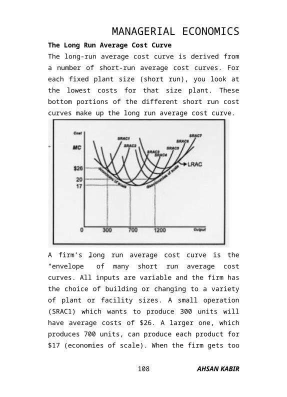
MANAGERIAL ECONOMICS

The Monopolist’s Average Revenue and Marginal Revenue CurvesAverage revenue, by definition, is equal to the price of the product, so the AR revenue curve is the same as the demand curve. The MR curve is in a different location, however. It is downward sloping and lied below (it’s steeper) than the demand curve.

The following example shows that in a monopoly market the MR is always less than price. A monopolist produces 100 newspapers (sometimes a newspaper firm can hold a local monopoly) at a price of $.50. It can also sell 120 newspapers at $.45 per paper; or 140 at $.40. Notice that when the price changes to $.45 and $.40, the marginal revenue drops to $.20 (4/20) and $.10 (2/20) respectively. To check this, calculate the total revenue at output 100: TR = P x Q = $.50 x 100 = $50. At output 120, TR is: $.45 x 120 = $54. So the marginal revenue equals $4 (the increase in total revenue) divided by 20 (the increase in output) or $.20. Similarly, the marginal revenue from output 120 to 140 equals $2 divided by 20 or $.10.

The Monopolist’s Profit Maximizing (Loss Minimizing) SituationSimilar to the pure competition case, a monopolist maximizes profits by finding out where MC and MR are

AHSAN KABIR108

MANAGERIAL ECONOMICSequal or almost equal (still contingent upon MC not exceeding MR; MC must not be falling; and price must be at least as great as AVC).Remember that profit is TR – TC and average profit is price (AR) minus ATC. Also note that even though monopolists often make profits, there is no guarantee that they alwaysdo.

Application: Given the above demand and cost data for a monopolist who sells economics textbooks, what are the profit maximizing output, price, and profit for this form?Answer: Output = 600 units, Price = $32, Profit = $19,200 – $ 15,000 = $4,200, Average Profit = $7

Monopolistic Competition

Characteristics of a Monopolistically Competitive Industry

AHSAN KABIR109

MANAGERIAL ECONOMICSFour characteristics of monopolistic competition are:

1. There are many sellers in this industry (lots of competition)

2. It’s easy for firms to enter this industry and for existing firms to exit

3. Firms in this industry sell differentiated products4. Firms in this industry frequently advertise

(usually on a local level).

Characteristics 1 and 2 are the same as in perfect competition. Characteristic 3 means that firms in this industry sell products that are similar but slightly different. The difference may lie in the packaging of the product, the ingredients, the service associated with the product, the name of the product, or the difference may even be only perceived by consumers.

The advertising (characteristic 4) helps to emphasize these differences to consumers. These last two characteristics also mean that firms in this industry do not all have to charge the same price for the product. Since the products are slightly different they can change different prices. The demand curve is therefore downward sloping.

These are good examples of monopolistically competitive industries:

a. Retail clothing stores

e. Car dealers

AHSAN KABIR110

MANAGERIAL ECONOMICSb. Video rental stores f. Pizza restaurantsc. Gas stations g.Financial consulting

servicesd. Fast food restaurants

h. Legal services

Long Run Price and Output EquilibriumBecause there are no barriers to entry into this type of industry, a firm will not be expected to make economic profits in the long run. If (for a short while) a firm is making above normal (=economic) profits, then other firms would quickly enter this industry in order to share in the profits. The profitable firm’s sales would suffer and in the long run its economic profits would be zero. The reverse occurs when firms lose money.

Monopolistic Competition as a More Realistic ModelAs you can judge from the characteristics, the model of monopolistic competition is more realistic than the purely competitive one. All firms, small or large, differentiate, if not through different ingredients, certainly in the way that they package, name, distribute, or service their products. Advertising is also very common; it benefits the firm because of the greater exposure to a larger market and often benefits the consumer by informing her/him of the choices available.

AHSAN KABIR111

MANAGERIAL ECONOMICSMonopolistically competitive firms earn “normal” accounting or so-called “zero” economic profits. Firms look at their cost of production and then mark up their prices to obtain a reasonable percentage profit. If any firm marks up its prices too much, another firm will take advantage of it by changing a slightly lower price. This will cause the first firm to lose market share and the mark-up will be adjusted accordingly. This competitive process occurs in any industry, monopolistic competition, oligopoly or monopoly, as long as there is free, unrestricted (from government legislation) competition. It is rare therefore to see a firm in any unrestricted industry experience exorbitant, above normal economic profits for an extended, long term period of time.

OligopolyCharacteristics of an Oligopoly IndustryOligopoly industries are characterized by:

1. Few (two, three, four, …) sellers who control all or most sales;

2. Barriers to entry (it is difficult to start a new company in an oligopoly industry);

3. Firms in this industry are interdependent (one firm’s actions very much affect a rival firm’s well being);

4. Advertising is prevalent (firms frequently advertise on a national scale).

AHSAN KABIR112

MANAGERIAL ECONOMICSOligopoly firms are usually large relative to the market in which they operate. Consequently, if one oligopoly firm changes its product price or alters another part of its marketing strategy, it will significantly impact the rival firm(s). For instance, if Pepsi lowers its prices to 50¢ per can, Coke will be affected. Coke most likely will lower its price, too. If this happens neither company will gain a competitive advantage.

These markets are good examples of oligopoly industries:

a. The automobile industry e. The beer (wholesale) industry

b. The airline industry f. The cereal (breakfast) industry

c. The photographic equipment industry

g. Infant formula makers

d. The aircraft manufacturing industry

h. The oil industry (OPEC)

Collusion and Barriers to Collusion in OligopoliesWhen firms collude and behave in a monopoly like fashion they will be able to restrict output and charge a higher price. Each firm will see its profits increase in the short run as companies engage in price setting (fixing) and cooperate to keep out competitors. Collusion and cartels are not legal in many countries

AHSAN KABIR113

MANAGERIAL ECONOMICSincluding the US and the UK. In contrast, legal cartels in some countries are fairly common. The most famous example of an international cartel is OPEC (Oil Producing and Exporting Countries). Collusion among producers and retailers may occur legally (outside the U.S.) or covertly. However, cartels frequently run into problems for the following reasons:

1. Cartel members’ interests and goals may differ. This makes it very hard to reach an agreement between members. For instance, in the case of OPEC, Saudi Arabia, Iran, Iraq, Kuwait and other nearby countries have long fought (recently very literally) about how much to produce and what price to charge. The fierce disagreement between Iraq and Kuwait in July of 1990 triggered the war which broke out the following month. Another OPEC country, Venezuela, is interested in maintaining a high price and restricting output to preserve its smaller holdings of oil for a longer time.

2. Even if an agreement has been reached it is tempting for members to secretly cheat and supply more at the very high monopoly price in order to increase revenue. Of course if all

AHSAN KABIR114

MANAGERIAL ECONOMICScountries cheat and increase supply the effect of a cartel is completely lost.

3. At the very high cartel price it becomes increasingly attractive for new producers to enter the market. In the oil market this has indeed occurred. After the price of a barrel of oil reached $34 in the late ‘70s, other countries found it profitable to drill and export oil. England, Mexico, Norway, the United States, and Russia entered the market and through their competition drove down the price of oil. During the 1980’s and early ‘90s the average price of a barrel of oil has indeed come down and it has made OPEC’s life a lot more difficult.

The above examples illustrate that, in the long run, given free and unrestricted competition, no firm, whether oligopolistic or monopolistic, can be expected to earn above normal profits. Competitive market forces prevail and ensure a fair price to consumers.

Questions for discussions

Questions for discussion1. What are the characteristics of perfect

competition?

AHSAN KABIR115

MANAGERIAL ECONOMICS2. Explain the rule for profit maximization (or loss

minimization for a perfectly competitive firm.3. What is imperfect condition? Mention different

types of imperfect competition.4. What are the characteristics of oligopoly and

monopolistic competition?5. Write a note on the collusion and barriers to

collusion in an oligopolistic market.

Nine: Issues in Pricing

Introduction

AHSAN KABIR116

MANAGERIAL ECONOMICSNone is more critical to the success of a firm than setting the price of output. The immediate and obvious effect of pricing choices is reflected in short-run profits. But prices set today can also have an important impact on future profits. The pricing decision often appears deceptively simple. If the firm has some control over price, the rule is to produce until marginal revenue equals marginal cost (MR = MC) and charge the price indicated by the demand curve (or Average revenue) for that quantity. As always, economic theory involves simplifications of reality. A large corporation might produce several hundred products that are sold in many different markets. Sometimes, the price set for one of these products can affect the demand for other products sold by the firm. For example, the price the Gillette Corporation sets for razors may affect the quantity of blades demanded that fit these razors, and vice versa. Similarly, production decisions relating to one product may affect the manufacturing or marketing costs of other products.

Pricing of Multiple Products

Procter & Gamble began in 1837 as a partnership selling soap to residents of Cincinnati, Ohio. Today, the firm has annual sales of over $30 billion and sells hundreds of products throughout the world. Procter &

AHSAN KABIR117

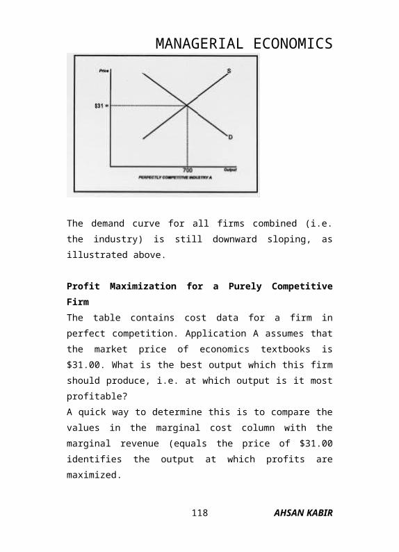
MANAGERIAL ECONOMICSGamble's most popular brands are shown in the following Table.

Laundry and Cleaning Products

Personal CareProducts

Food Products

Cascade Bounty CriscoCheer Camay CrushComet Charmin Duncan

HinesDash Crest Folger'sDowny Head &

ShouldersHires

Ivory Liquid Ivory Soap JifMr. Clean Luvs Pringle'sSpic and Span PampersTide Pepto-Bismol

Some of these products are unrelated. For example, the demand for Pringle's Potato Chips is unlikely to be affected by the price of Tide. Similarly, production costs of Pringle's are independent of the amount of Tide produced. However, demand and production of other Procter & Gamble brands are interrelated. Clearly, Luvs and Pampers would be considered substitutes by consumers of disposable diapers. As such, the price of Luvs affects the demand for Pampers and vice versa.

AHSAN KABIR118

MANAGERIAL ECONOMICSAlso, the two competing brands share the same production facilities. Thus, if pricing decisions are based partially on costs, prices will be dependent on how costs are allocated between the two products.

When firms produce several products, managers must consider the interrelation ships between those products. Pricing techniques for multi-product firms are considered in this section.

Products with Interdependent DemandsProducts with interdependent demands are either substitutes or complements. For substitutes, such as Luvs and Pampers, a price increase for one good tends to increase the demand and for the other. However, the magnitude of the increase also depends on the number of substitutes available from other suppliers. For goods that are complements, a price increase tends to reduce the demand for the other good. Options that can be added to new cars are a good example of complements. Sales of antilock brakes, power windows, and stereo systems by an automobile manufacturer are dependent on the number of vehicles sold by the company. If the price of the basic automobile is in creased, vehicle sales will decline, and the demand for options will also decrease.

AHSAN KABIR119

MANAGERIAL ECONOMICSCorrect pricing decisions require that demand interdependencies be taken into account. Instead of setting each price in isolation, the impact of each price on the demand for other products produced by the firm must be considered. The basic objective of the manager should be to determine prices that maximize total profit for the firm rather than only profit earned by individual products.

A firm may produce two separate products. And those two products can either be with independent demand or interdependent demand for them. In case the products are demanded independently of each other, the profit maximizing price for both of them will be determined separately as if they were produced by different firms.

On the other hand, if the products have interdependent demand, then the pricing policy will be different. To find the profit-maximising price for a good, we follow the condition of equality between marginal revenue (MR) and marginal cost (MC).

When demands are interrelated, insight into managerial decisions can be gained by considering the marginal revenue equations for the products. Assuming that the MC for both products is the same, we need to determine the Mr functions for both goods separately. Consider a firm that produces only two goods, X and Y Assume that

AHSAN KABIR120

MANAGERIAL ECONOMICSsales of X have an impact on the demand for Y and vice versa. In terms of marginal revenue, this assumption can be stated mathematically as,

the MR for Good X is given by the following equation,

MRX = dTRX / dQX + dTRY / dQX

(i)

Similarly, the MR for Good Y is as follows,

MRY = dTRY / dQY + dTRX / dQY

(ii)

Equation (i) indicates that marginal revenue associated with changes in the quantity of X can be separated into two components. The first, dTRX / dQX represents the change in revenues for good X resulting from a one-unit increase in sales of good X. The second, dTRY / dQX

reflects demand interdependency. It indicates the change in revenue from the sale of good Y caused by a one-unit increase in sales of good X. Now, if the goods are complementary, the sign of the second term in each of the above equation will be positive, and if substitute, the sign will be negative.

Clearly, the firm must consider demand interdependencies in order to make optimal pricing and

AHSAN KABIR121

MANAGERIAL ECONOMICSoutput decisions. Assume that goods X and Y are complements, In determining the profit-maximizing rate of output for good X, if the effect of sales of X on the demand for Y is not considered, output of X would be increased only until dTRX / dQX equals the marginal cost of producing X. But, as can be seen from equation (i), dTRX / dQX understates the actual incremental revenue generated by selling an additional unit of X. Specifically, revenue also is affected by dTRY / dQX, which is positive if the two goods are complements. Thus, when demand interdependence is taken into account, profit maximization requires a greater rate of output for good X In fact, output of X should be increased until,

dTRX / dQX + dTRY / dQX = MCX

Therefore, the profit-maximising condition for good X is,

MRX = dTRX / dQX + dTRY / dQX = MCX

(iii)

where MCX is the additional cost incurred by the firm in producing an additional unit of good X. Similarly, for goods that are substitutes, it can easily be shown that ignoring the demand interdependency will cause too many units of output to be produced.

Similarly for good Y, the profit maximising condition is,

AHSAN KABIR122

MANAGERIAL ECONOMICS

MRY = dTRY / dQY + dTRX / dQY = MCY

(iv)

An Example: Turkey Prices at ThanksgivingFor most American families, roast turkey is an important part of their Thanksgiving festivities. Although pumpkin pie, potatoes and gravy, and cranberry sauce are a traditional part of the meal, it is the size and taste of the turkey that determine the quality of the dining experience.

For many years, most families ate turkey only at Thanksgiving and Christmas. Today, turkey is recognized as a highly nutritious and relatively inexpensive meat and is eaten throughout the year. Turkey consumption has risen from 5.5 pounds per capita during the 1950s to about 20 pounds per person in the late 1990s. However, demand for turkey still increases dramatically in November and December as families prepare for the holidays.

Economic theory predicts that when the demand for a product increases, the price should also increase. This is exactly what happens at the wholesale level. In early November, turkey producers raise their prices in anticipation of increased purchases by grocery stores

AHSAN KABIR123

MANAGERIAL ECONOMICSand restaurants. For example, in 1997, the average wholesale price of turkey was 72 cents per pound. But during the fourth quarter of that year, the wholesale price averaged 75 cents.

Higher wholesale prices for turkey should result in a higher price at the retail level, but this is not the case. Typically, the price that shoppers pay for turkey is actually less around Thanksgiving and Christmas than during the rest of the year. The reason is that turkey is often used as a loss leader to entice customers into the store. Retailers assume that any losses they experience on turkey can be more than recouped as shoppers buy all of the other items that they need for the holiday season. Basically, the store owners recognize the interdependence between the demand for turkey and the other products they sell. Because of this complementary relationship, turkey prices are kept low.

Pricing of Joint ProductsProducts can be related in production as well as demand. One type of production interdependency exists when goods are jointly produced in fixed proportions. The process of producing beef and hides in a slaughterhouse is a good example of fixed proportions in production. Each corpse provides a certain amount of meat and one hide. There is little that the

AHSAN KABIR124

MANAGERIAL ECONOMICSslaughterhouse can do to alter the proportions of the two products.

When goods are produced in fixed proportions, they should be thought of as a "product package." Because there is no way to produce one part of this package without also producing the other part, there is no conceptual basis for allocating total production costs between the two goods. These costs have meaning only in terms of the product package. Although the two goods are produced together, their demands are independent. However, there is a single marginal cost for both products. This reflects the fixed proportions of production, that is, the marginal cost is the cost of supplying one more unit of the product package.Where goods are jointly produced, pricing decisions should take this interdependency into account. When an additional animal is processed at a slaughterhouse both the beef and the hide become available for sale. Hence, the marginal revenue associated with sale of a unit of the product package is the sum of the two marginal revenues.

Example Calculating the Profit-Maximizing Prices for Joint ProductsA rancher sells hides and beef. The two goods are assumed to be jointly produced in fixed proportions. The

AHSAN KABIR125

MANAGERIAL ECONOMICSmarginal cost equation for the beef-hide product package is given by

MC = 30 + 5QThe demand and marginal revenue equations for the two products are

BEEF HIDESP = 60 - 1Q P = 80 - 2Q

MR= 60 - 2Q MR = 80 - 4Q

What prices should be charged for beef and hides? How many units of the product package should be produced?

SolutionSumming the two marginal revenue equations gives

MRT = 140 - 6Q

The optimal quantity is determined by equating MRT and MC and solving for Q. Thus

MRT = MCOr, 140 - 6Q = 30 + 5Q

and hence, Q = 10Now, substituting Q = 10 into the demand curves yields a price of $50 for beef and $60 for hides. However, before concluding that these prices maximize profits, the marginal revenue at this output rate should be computed for each product to assure that neither is negative. Substituting Q = 10 into the two marginal

AHSAN KABIR126

MANAGERIAL ECONOMICSrevenue equations gives $40 for each good. Because both marginal revenues are positive, the prices just given maximize profits. If marginal revenue for either product is negative, the quantity sold of that product should be reduced to the point where marginal revenue equals zero.

Intermediate Products (Transfer Pricing)Vertical integration is common in modern economic systems. A firm is said to be vertically integrated when it operates at more than one stage of the production process. For example, some steel producers mine coal and iron, transport the ore on boats owned by the firm, use the coal as an energy source to transform the iron into steel ingots, shape the steel ingots into finished products, and distribute those finished products to consumers. The fabricated steel products received by the consumers are final goods. In contrast, the coal, iron ore, steel ingots, and undelivered steel products are referred to as intermediate goods. That is, they are goods or materials that will be needed as inputs at a later stage of the firm's operations.By taking advantage of scale economies, avoiding possible supply disruptions, and bringing complementary aspects of the production process together a vertically integrated company may be more efficient than several small firms, each operating at a single stage of the production process. However,

AHSAN KABIR127

MANAGERIAL ECONOMICSgreater size resulting from vertical integration can cause control problems. Top management may find it difficult to become familiar with each stage of the operation or a cumbersome bureaucracy may develop that makes it difficult to implement decisions.

One method of dealing with such problems is to organize vertically integrated firms into semi-autonomous divisions. Each of these divisions has its own function and its own management. Each management team is rewarded based on the performance of the division. In some cases, the evaluation is based on the profit earned by the unit. In an integrated firm, determining the amount of profit that should be credited to a division producing an intermediate product is a difficult task. The problem is that if the unit's function is to provide an input for the next stage of the production process, revenue will depend on the price that is charged for the intermediate good. A high price will increase profits of the unit at the earlier stage of production, whereas a low price will make the later production stage appear more profitable.

A more serious problem is that an incorrect price set for an intermediate good can affect the total profit earned by the firm. Specifically, if the decision makers in each division attempt to maximize profits for their units, the total profit of the firm might be reduced. Thus, it is

AHSAN KABIR128

MANAGERIAL ECONOMICSimportant that prices of intermediate products be set to maximize overall profits rather than division profit. This objective may require that top-level management be involved in pricing intermediate goods.

The following discussion provides guidelines for the pricing of intermediate products, sometimes referred to as transfer pricing. For simplicity, it is assumed that there are only two stages of production. In the first, rolls of paper are manufactured as an intermediate product. In the second, paper is cut into writing tablets and sold to final consumers. Two alternative situations are considered. The first occurs when an external market exists for the intermediate good. That is, the division making rolls of paper can sell its output to buyers outside the firm, and the unit requiring the paper has alternative sources of supply. The second case is when there is no external market and paper can be bought and sold only between the two divisions of the firm. In this case, there is no market-determined price for the rolls of paper.

External Market. Assume that the writing tablet division of the integrated firm has the option of obtaining paper from the paper manufacturing division or from in-dependent suppliers. Similarly, the paper manufacturing unit can sell to the writing tablet division or to other buyers. Also assume that the external

AHSAN KABIR129

MANAGERIAL ECONOMICSmarket is perfectly competitive. This implies that the two units can buy or sell as much as they want at the market-determined price.

With a perfectly competitive external market, there really is no price decision to be made. The paper manufacturing unit, like a competitive firm, faces a horizontal demand curve at the market-determined price (assuming a perfectly competitive market). If the managers of that unit attempt to maximize profits, they will increase production until price equals marginal cost (or P = MC). If the paper manufacturing division tries to charge a price in excess of the market price, the writing tablet unit should buy paper from independent suppliers. If the final product division is unwilling to pay the market price, the paper rolls can be sold on the open market.

Where an external market exists, it is not necessary that the output of the paper manufacturing division equal the input demand for the tablet unit. If there is an excess supply of paper rolls, it can be sold to other firms. Similarly, if the firm's internal supply of paper is insufficient, the tablet division can buy from other producers.

No External Market. If no external market exists or if the divisions are not allowed to trade with other firms, a

AHSAN KABIR130

MANAGERIAL ECONOMICSconflict may arise regarding the proper price to be charged for paper. The paper manufacturing unit may benefit from a higher price, while the division that makes tablets may benefit from a lower price. However, the goal of top management is to determine the Price for paper that results in maximum profit for the com-bined firm. In this case, profit maximization requires that the price of each intermediate good be set equal to its marginal cost.

Price DiscriminationFrequently, the same book is sold at a much lower price in South America and Europe than in the United States. This practice is an example of price discrimination and is designed to increase the total profit of the book publisher. From an economic perspective, price discrimination occurs when price differences between consumers or markets do not reflect variations in the cost of supplying the product.

Sometimes price discrimination involves charging a uniform price when costs differ. Consider the firm that advertises an all-you-can-eat buffet for $9.95. The first customer is a jockey who does little more than pick at the salads. The second is an NFL defensive tackle, who requires 10,000 calories a day just to maintain his body weight. The uniform price of $9.95 constitutes price

AHSAN KABIR131

MANAGERIAL ECONOMICSdiscrimination because the cost of serving the two customers differs markedly.

More commonly, price discrimination occurs when prices differ even though costs are essentially the same. Physicians' services are an example. For a given treatment, there is no reason to believe that costs depend on the income of the recipient. Yet high-income patients are sometimes charged more than the poor for the same services.

Necessary Conditions for Price DiscriminationThree conditions must be met before a firm can successfully practice price discrimination. First, the firm must have at least some control over price. Obviously, a price-taker in a perfectly competitive market is not in a position to engage in price discrimination. Second, it must be possible to group different markets in terms of the price elasticity of demand in each. It will be shown later that firms can increase total profit by charging relatively higher prices in markets where demand is less elastic.

Finally, the firm's markets must be separable, meaning that products cannot be purchased in one market and then resold in another. Suppose that a firm has identified two markets and charges a high price in the first and a lower price in the second. If the two markets

AHSAN KABIR132

MANAGERIAL ECONOMICSare not separable, price discrimination cannot be successful. Either consumers will go to the low-priced market and make their purchases, or enterprising individuals will buy in the low-priced market and resell at a price below that is established by the firm in the high-priced market. In either case, the price differential between the markets will disappear as prices decline in the first market and increase in the second.

Price Discrimination and the AirlinesFinding the lowest airfare can be a puzzling experience. On any given day, there are tens of thousands of different fares available. With a full 150-seat aircraft flying between two U.S. cities, it would not be uncommon for the passengers to have paid 20 different fares for their seats. In some cases, these differences at least partially reflect amenities associated with higher price tickets. For example, first-class passengers have more leg room and better meals. But in other cases different prices are charged for the same travel ex-perience. During the summer, a regular coach round-trip ticket from Chicago to San Francisco costs as much as $900, but promotional pricing by the airlines allow some passengers to make the same journey for only $300. Once on board the plane, service was identical, same cramped seats, same bland meals, and same inconvenient rest rooms.

AHSAN KABIR133

MANAGERIAL ECONOMICSFor many years, the airlines have used what they call yield management to increase their profits. This practice involves both price discrimination and marketing. The price discrimination component is based on variations in price elasticities for different types of customers. Typically, business flyers have less elastic demands because they must meet with suppliers and customers at specific times and in specific locations. Of-ten, these trips are made on relatively short notice. Airlines take advantage of this situation by setting higher prices for tickets that do not require advance purchase. In contrast, vacation travelers often choose between many destinations (including some that do not involve air travel) and plan their trips far in advance. Because these discretionary travel demands are more price sensitive, airlines advertise some seats at lower prices if passengers are willing to buy their tickets 7 to 30 days in advance.

Types of Price DiscriminationThere are many forms of price discrimination, but the standard method of classification identifies three types or degrees of discrimination. Their common characteristic is that they allow the firm to capture part of the consumer surplus that would have resulted from uniform pricing.

First-Degree Discrimination

AHSAN KABIR134

MANAGERIAL ECONOMICSFirst-degree price discrimination involves charging the maximum price possible for each unit of output. Thus, the consumer who attaches the greatest value to the product is identified and charged a price of P1. Similarly, the consumers willing to pay P2 for the second unit and P3 for the third are identified and required to pay P2 and P3, respectively.

First-degree discrimination is the most extreme form of price discrimination and the most profitable pricing scheme for the firm. Because buyers are charged the maximum price for each unit of output, no consumer surplus remains. Consumer surplus is the difference between the price a consumer is willing to pay and the actual price charged for the good or service. The maximum consumer surplus occurs when there is no price discrimination and price is set equal to marginal cost.

First-degree discrimination is not common because it requires that the seller have complete knowledge of the market demand curve and also of the willingness of individual consumers to pay for the product. In addition, the seller must be able to segment the market so that resale between consumers cannot take place. These requirements are seldom met in actual market situations. However, one possible case involves the sale of the Treasury Bonds by the federal government. In

AHSAN KABIR135

MANAGERIAL ECONOMICSselling these bonds, the government requires each prospective buyer to submit a sealed bid. Those conducting the auction determine a minimum bid. All the bids that exceed the minimum are accepted and the bidders are obligated to buy at the price they indicated in their bid. Thus, through this process, the government attempts to extract the maximum price that each buyer is willing to pay.

Second-Degree DiscriminationSecond-degree price discrimination is an imperfect form of first-degree discrimination. Instead of setting different prices for each unit, it involves pricing based on the quantities of output purchased by individual consumers. For each buyer, the first Q1 units purchased are priced at P1, the next (Q2 – Q1) units are priced at P2, and all additional units are priced at P3.

In most cases, second-degree price discrimination involves goods and services whose consumption is metered. Electricity is an example. Many electric utilities use a declining-block tariff in pricing electricity. A typical tariff might specify the following monthly rates for blocks of usage:

First 100 kilowatt-hours $0.12 per kwhNext 300 kilowatt-hours $0.10 per kwh

AHSAN KABIR136

MANAGERIAL ECONOMICSAll additional kilowatt-hours $0.08 per kwh

It should be observed that just because different prices are charged for different blocks of consumption, it does not necessarily imply second-degree price discrimination. The high rate for the first 100 kilowatt-hours may be intended to recover the fixed costs of serving a customer, such as billing and metering. As such, the $0.12 for the first 100 kilowatt-hours may not involve price discrimination. But if kilowatt-hours beyond 300 cost the utility the same amount to provide as those in the second block, then price discrimination is being practiced.

In addition to electricity, second-degree price discrimination is often used in setting rates for water, gas, and time-share computer usages in cyber cafes. It is also practiced by fast-food establishments. For example, a seller may offer soft drinks for $1.00, with refills available at $0.50. This pricing policy reflects the fact that the second drink is less valuable to the customer and will be purchased only at a lower price.

Third-Degree Discrimination The most common type of price discrimination is third-degree discrimination. It involves separating consumers or markets in terms of their price elasticity

AHSAN KABIR137

MANAGERIAL ECONOMICSof demand. This segmentation can be based on several factors. Often, third-degree price discrimination occurs in markets that are geographically separated. The practice of selling books at a lower price outside the United States is an example. Evidently, buyers in other countries have greater elasticities of demand than do U.S. buyers. At the same time, costs of collecting and shipping books make it unprofitable for other firms to buy in foreign countries and resell in the United States.

Discrimination can also be based on the nature of use. Telephone customers are classified as either residential or business customers. The monthly charge for a phone located in a business usually is somewhat higher than for a telephone used in a home. The explanation is that business demand is less elastic than residential demand. An individual without a telephone may be able to use a pay phone or go to a neighbor’s house to make a call, but for many businesses a telephone is an absolute necessity.

Finally, markets can be segmented based on personal characteristics of consumers. Age is a common basis for price discrimination. Most movie theatres charge a lower price for children than they do for adults. But there is no difference in the cost of providing service to the two groups – one seat is required for each patron regardless of age. The reduced price for children is

AHSAN KABIR138

MANAGERIAL ECONOMICSbased on differing demand elasticities. The assumption is that, with less money to spend a child's demand for movies is more price sensitive than an adult's.Questions for discussions

1. Why do you think pricing decision is so important for any firm?

2. Briefly explain the issue of pricing multiple products by a firm.

3. With the help of an example, elaborate what should be the optimum pricing policy for a firm producing joint products?

4. What is transfer pricing? How does it take place in different situations?

5. Explain different types of price discriminations with examples.

AHSAN KABIR139

MANAGERIAL ECONOMICS

AHSAN KABIR140

MANAGERIAL ECONOMICS

Module: Managerial Economics

Lecture Ten: Technological Change in an Economy

IntroductionChanges occur so rapidly in the modern society that many businesses find it difficult to adapt to their evolving environment. The average person is emotionally and intellectually left behind by the rapid pace of technical and cultural change. If this idea had any relevance for the last century, it is even more applicable as society moves into the new millennium. The last two decades brought radical changes in world political alignments, different societal values, and the availability of thousands of new and improved products because of advances technology.

Faced with rapid change, many firms have found it difficult to keep pace with it. The demise of communism opened new markets in the former Soviet Union and Eastern Europe, but also reduced the demand for some products (such as military hardware) and intensified global competition. Complicating the situation is the need for firms to stay abreast of new developments within their own industry. Electronics companies must be competitive using the new digital technologies for their audio and video equipment. Automobile

AHSAN KABIR141

MANAGERIAL ECONOMICSmanufacturers survive only if they keep costs down by using advanced robotics for assembly. Computer suppliers can stay profitable only if their machines include state-of-the-art chips, display terminals, and storage devices.

The impact of technological changeTechnological change may involve new products, improvements or cost reductions of existing products, or better ways of managing the operations of a business. In some cases, the changes may seem simple and the results rather trivial, such as coating paper clips with coloured plastic to prevent them from leaving marks on a page or tapering one side of the buttons on a shirt to make them easier to fasten.

In other cases, the technological advance may be brilliant and the impact on society highly significant. Consider the development and evolution of the electron microscope. The best optical microscopes can focus on objects as small as 1,000 angstroms (a unit of measurement equal to one ten-billionth of a meter) in width. During the 1930s, scientists learned to focus streams of electrons in the same way that optical devices focus light. The first electron microscopes achieved resolution of about 100 angstroms -- ten times better than the optical microscopes. During the next 60

AHSAN KABIR142

MANAGERIAL ECONOMICSyears, research efforts significantly improved the instruments. Today, commercially available electron microscopes can focus on objects as small as one angstrom – thousand times better technology.

Technological Change, Productivity, and Economic GrowthEconomists use several measures to assess the performance of the economy. One of the most important measures is protectively, defined as the ratio of output to one or more inputs. Productivity is a key concept because it determines the standard of living that a country can achieve. In any given year, the total value of income received by individuals is based on the total value of goods and services produced. Thus, the only way for all consumers to have more real income is for the productivity of the inputs used to produce those goods and services to increase.

The most common productivity measure is labour productivity, total output divided by the quantity of labour. If labour productivity can be increased, workers may be able to earn higher wages. Labour productivity has increased over time. However, there have been significant differences between countries. Percentage changes in labour productivity between 1970 and 1989 are provided in the following table for selected

AHSAN KABIR143

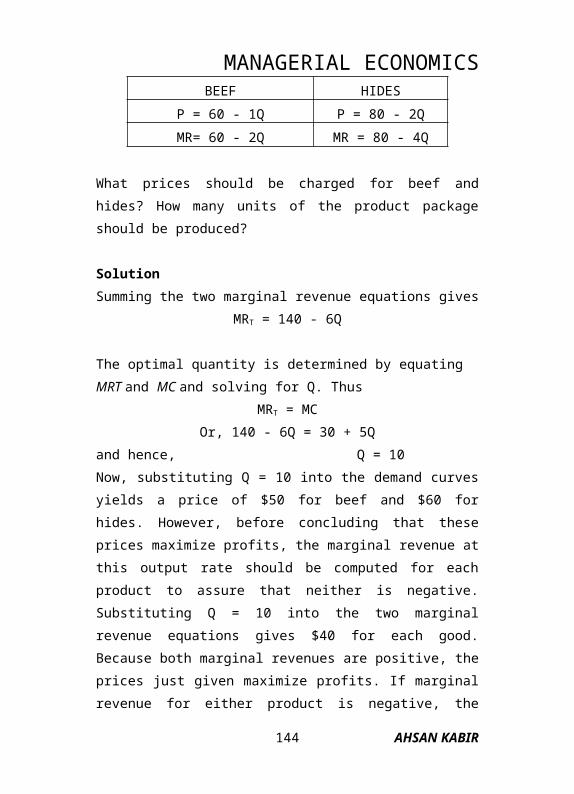
MANAGERIAL ECONOMICScountries. Note that the rate of increase for the United States is less than every nation except Canada and Sweden. Slow growth in labour productivity has been a concern in the United States in recent years.

Country Productivity change (%)

United States 2.9%Canada 2.5%Denmark 3.3%France 4.1%Italy 4.9%Japan 6.0%Netherlands 4.9%Sweden 2.9%United Kingdom 3.8%Germany 3.2%

Table: % increase in labour productivity

Technological change is an important source of increased labour productivity. Labour-saving technological change allows the same number of workers to produce more output. However, technological change is not the only component of increased labour productivity. Productivity increases as workers accumulate more human capital and as the capital stock of the economy increases. Changes in

AHSAN KABIR144

MANAGERIAL ECONOMICSrelative input prices can also affect the measured rate of labour productivity. If capital becomes relatively more expensive, for example, firms will use more labour and less capital. Thus, the ratio of output to labour input will decrease. Conversely, higher wage rates tend to reduce labour usage and to increase the measured rate of labour productivity.

The output-labour ratio is commonly used to measure productivity because it is easy to quantify. However, a better indicator is total factor productivity, which com-pares changes in output with changes in both labour and capital inputs. Using this approach, it is possible to identify the sources of economic growth over time. A study focused on economic growth as measured by the change in real income in the United States between 1929 and 1982. The average annual growth rate in real income over the period was 2.8 percent. The estimated components of growth are shown in the table below.

Source of Growth Percent Attributable to Source

Increase in inputs 53%Labour 20%

Education19%

AHSAN KABIR145

MANAGERIAL ECONOMICSCapital 14%

Technological change 31%Other factors* 16%

Total 100%*Economies of scale, improved worker safety, and health, pollution abatement, and fewer labour disputes

Note that the single most important source of economic growth between 1929 and 1982 was technological change. Almost one-third of the increase is attributable to improvements in technology. It is also important to observe that about 20 percent of growth was due to higher education levels of workers. Clearly, knowledge, whether associated with new or improved products or embodied in workers, is crucial to economic progress.

The effect of market structure on technological changeSome economists believe that market power is a necessary condition for rapid technological change. They argue that most modern research and development activities require huge investments and can take years before they yield results. Small firms operating in competitive markets may not have funds to allocate to such efforts and may be unable to take advantage of scale economies associated with complex R&D projects. Also, firms in competitive markets may

AHSAN KABIR146

MANAGERIAL ECONOMICSbe unable to capture all the economic profits resulting from their efforts. If competitors can easily imitate new products and product improvements, firms will be less likely to allocate their resources to R&D.

One of the most vocal advocates of this view is John Kenneth Galbraith. Using language reminiscent of Adam Smith's "invisible hand," Galbraith wrote in his book ‘American Capitalism (Boston 1952)

“A benign Providence ... has made the modern industry of a few large firms an almost perfect instrument for inducing technical change... There is no more pleasant fiction than that technical change is the product of the matchless ingenuity of the small man forced by competition to employ his wits to better his neighbour.... Technical development has long since become the preserve of the scientist and the engineer.

Clearly, large firms have been responsible for many important developments. AT&T's Bell Labs devised the transistor and Dupont introduced nylon. But small firms have also had an impact. Steven Jobs started Apple in his garage and revolutionized the computer industry. Photocopying was invented by a patent attorney, Herbert Carlson, and commercialized by a small firm that later became the Xerox Corporation. A study

AHSAN KABIR147

MANAGERIAL ECONOMICSinvestigated the origins of 70 major inventions since 1880. It found that 54 percent of those inventions could be attributed to people working alone and another 11 percent involved individuals working with research institutions. Only about one-third of the inventions came out of industrial research laboratories.

The case can be made that small firms in competitive markets might be more progressive than larger firms with monopoly power. Small firms may be more likely to provide an environment in which new ideas can flourish, while larger firms may impose bureaucratic rules that suppress creativity. Also, a young, small firm may have to be innovative to survive. In contrast, large, established firms that are partially insulated from competition may have very little motivation to change their product lines or production methods.

In evaluating the effect of market structure on technological change, the key is to consider both the ability and the incentives to be progressive. Ability involves being able to fund expensive R&D projects, withstand failures, and wait for results. Incentives include the need to remain competitive and being able to capture the rewards of technological advance.

The Effect of Technological Change on Market Structure

AHSAN KABIR148

MANAGERIAL ECONOMICSMarket structure can affect the rate of technological change, but technology can also significantly affect the structure of the market. Telecommunications is a good example. The basic telephone patent was issued to Alexander Graham Bell in 1876. This right made the Bell System a monopoly until it expired in 1893. For a few years, there was vigorous competition in some cities, but the available technology soon caused the industry to evolve into a virtual monopoly. In each city, the local network required that lines be deployed to every home and business in the community. This in-volved obtaining rights of way, putting wires under streets, and erecting thousands of telephone poles. Establishing a nationwide long-distance network required that tens of thousands of miles of copper wire be run over great distances and through often difficult territory. The necessary capital equipment was extremely expensive and there were significant economies of scale associated with the endeavour. As a result, smaller firms were unable to compete, and AT&T was the dominant firm for almost one hundred years.

In the late 1960s, development of microwave technology provided opportunities for competitors. As an alternative to running cable, firms could establish communication links by setting up microwave towers every twenty or thirty miles. Microwave Communications Inc. (MCI) offered the first serious

AHSAN KABIR149

MANAGERIAL ECONOMICSchallenge to AT&T by offering data transmission service between St. Louis and Chicago. After ten years in court and numerous challenges to federal Communications Commission, MCI finally established itself as a viable competitor. Moro recently satellites and fibre optics have emerged as alternative technologies. Today, AT&T still dominates the long-distance market, but it faces significant competition from firms such as MCI and Sprint.

Some casual observers of the industry have suggested that the recent dramatic change in telecommunications market structure are primarily the result of changes in regulatory policy, as the courts and Federal Communications Commission have permitted competition in markets where monopolies had been protected. But a closer examination reveals that government was simply responding to the forces of technological change. When telecommunications technology no longer dictated the existence of natural monopoly, it was impossible for bureaucrats to perpetuate this structure. The new technologies made increased competition inevitable.

The same forces have caused structural change in the computer industry. Technological change has resulted in faster computer chips and storage devices. This has changed the market because many applications that

AHSAN KABIR150

MANAGERIAL ECONOMICSpreviously required a large mainframe computer can now be performed on personal computers. The result is that the industry has evolved from an oligopoly dominated by a few firms such as IBM into a competitive market with hundreds of firms selling personal computers. As with telecommunications, the new market structure reflects changes in technology.

Invention, innovation and diffusion To this point, the term technological change has been used rather loosely. Sometimes it can be useful to distinguish among invention, innovation, and diffusion. Invention can be thought of as the creation of new ideas. Innovation represents taking those ideas and transforming them into something that is useful for society. Diffusion is the process whereby the new product or process becomes available throughout the society.

Again, innovation can be divided into two broad categories. Product innovation involves the bringing of new goods or services to the market, while Process innovation is concerned with new techniques that reduce costs of producing and distributing existing products.

Innovation, Technological Change and the Economy

AHSAN KABIR151

MANAGERIAL ECONOMICSAs the economy has moved from the industrial age to the information age, the driving force of innovation has excited some and frightened others. Personal computers, fibre optics, communication satellites, the World Wide Web and a host of other fascinating ideas have changed the way we work and play. Seemingly overnight, new industries have popped up with a host of new jobs to offer, while obsolete industries and jobs have gone by the wayside. The paradox that innovation is both central to economic progress and, at the same time, the cause of many economic difficulties is called the churn. The churn can be frightening to those whose lives may change because of new technologies, but we should remember that change is necessary for progress. Our challenge is to be prepared for the opportunities it affords us.

The U.S. Economy: An example of transformationIn the not-so-distant past, possessing physical strength was a sure way to get a job. Farmers trudged behind their ploughs, pick-and-shovel labourers clawed at the earth and loading dock workers slung cargo over their shoulders. But the economy has changed dramatically over the past 100 years.

In the early 1900s, machines began to reshape the role of workers in producing goods and services as the United States moved from the agrarian (or farming) age

AHSAN KABIR152

MANAGERIAL ECONOMICSinto the industrial age. Steam power, internal combustion engines and electric motors took the place of brute strength, and motor skills replaced muscle power as a worker's most valued resource. People learned to use tractors, backhoes, forklifts, cranes, lathes and other devices that saved time and energy. Soon, technology advanced even further, and machines themselves began taking over more factory chores.

Today, jobs rely even less on muscle power and motor skills. America has entered the information age, and brain power—analytical reasoning, creativity, inventiveness and even humour—has surpassed motor skill as the economy's most valuable labour resource. The emergence of computer, telecommunications and satellite technologies has dramatically changed the way Americans work. It now takes only a few employees to accomplish what once required dozens. For example, the number of secretarial jobs has been declining since the late 1980s because computers and laser printers allow supervisors to type and print their own letters and memos. Even in manufacturing plants, increasingly intelligent computers are taking on mundane tasks, such as those on an auto assembly line that once required workers' constant attention.

There is nothing new about all of this change. Innovation and the competitive spirit of the free

AHSAN KABIR153

MANAGERIAL ECONOMICSenterprise system have always made jobs, and even entire industries, obsolete. As competition grinds onward, as businesses open, close, expand, contract or relocate, they set in motion both layoff activity and new hiring. A shorthand term for the turbulence in the labour market that is caused by innovations or new ideas is the churn. The benefit of the churn is that innovation and technological advances free workers to perform other, more important tasks—creating new industries, new jobs and more goods and services for consumers to enjoy.

The Process of Innovation and CompetitonThe process of innovation and competition that recycles labour into new jobs is—more than ever—at work today. For example, there are more than 1.2 million computer programmers employed in the United States today. Among the fastest growing U.S. occupations in the 1980s were those of software designer, fax machine repairer and cellular telephone technician, jobs that scarcely existed 15 years ago.

Since the turn of the century, technological innovations have dramatically changed the way the American economy works. But for several reasons, such changes do not happen overnight.

AHSAN KABIR154

MANAGERIAL ECONOMICSFirst, the innovators themselves may not appreciate the usefulness of what they have created. For example, the inventor of the radio did not foresee that it would be useful for communicating to mass audiences. Rather, he saw it only as an improvement in two-way communications—from ship-to-ship or ship-to-shore. The steam engine, which played a huge role in igniting the industrial revolution, originally was invented by miners to pump water out of coal mines. They saw no other use for it at the time.

Second, an innovation may actually require another, complementary innovation before its usefulness can be appreciated. The laser, for example, was of little use to telephone companies until they also understood fibre optics. The combined potential of those two technologies, however, has transformed not only the telephone industry but also many others, such as cable television.

Finally, revolutionary new technologies, such as the telephone, electricity or the computer, take a long time to be fully integrated into the economy. For example, in 1910, only one-fourth of U.S. factories used electrical power. Most of these were limited to brand-new factories, while the older ones continued to rely on steam power. Twenty years later, three-fourths of factories used electricity.

AHSAN KABIR155

MANAGERIAL ECONOMICS

Time was needed to redesign and refit older factories for electrical power. All in all, it took about 40 years for electricity to become entrenched in American society and significantly affect U.S. productivity. This has exciting implications for the computer age, which began in 1970 with the invention of the microprocessor. Because the computer is even more complex than electricity, decades could pass before we realize the extent of the computer's potential. In other words, the greatest benefits of the computer may still lie ahead.

Adapting to ChangeThe transition from old industries to new ones can be bumpy and sometimes painful, especially for workers who lose their jobs. But the economy cannot progress without the revitalization that engenders job destruction. It may be tempting to save jobs because no one wants to face the struggles of unemployment. But government policies to save jobs almost always fail. They retard economic progress and ultimately destroy jobs by short-circuiting the vital process of innovation.For instance, had our ancestors been able to implement policies to freeze jobs, the United States might be stuck in the horse-and-buggy era. The former Soviet Union guarded the jobs of its citizens. Instead of spiralling upward with innovations, the Soviet Union stagnated and finally collapsed.

AHSAN KABIR156

MANAGERIAL ECONOMICS

The best approach a society can take is to learn to adapt to change. Change often makes people feel insecure. If people are insecure about their jobs because they do not feel their skills are up-to-date, then they will more likely fear job layoffs. Because the economy is changing so rapidly, ongoing schooling and training are becoming ever more necessary for workers. Today, a growing number of corporations realize the advantages of continuously training their workers. If ideas and brainpower are the most valuable labour resource, then training and education are crucial to a company's profitability. A well-educated, well-trained labour force more readily shifts from the jobs of declining industries to those of emerging ones. Education followed by constant re-education and training can bridge the gap between the skills of the past and those of value in the future.

Also important is a culture that embraces those who risk failure and loss to give the community something new or better than what was there before. These are the entrepreneurs. They are the people who have the energy and determination to discover new and better products and to risk taking those innovations to the market. Many are motivated by the desire to become rich and famous. Others are motivated by the desire to make the world a better place. Regardless of the goal,

AHSAN KABIR157

MANAGERIAL ECONOMICSconsumers benefit from new products and services, and workers benefit from new and exciting careers.

The world today possesses a large inventory of inventions to help plant the seeds of tomorrow's industries. The challenges for us lie in training workers for the jobs that will be created as these industries grow and in encouraging entrepreneurs to take the risks and endure the hardships and challenges associated with creating new and better products for the marketplace.

Questions for discussion1. Briefly discuss how can technological change

help shape the market structure?2. What is the impact of market structure on

technological change?3. Differentiate among invention, innovation and

diffusion.4. Explain how technological change can help

increase labour productivity. 5. Explain the importance of adaptation to changes

for an underdeveloped nation like Bangladesh.6. Why most of the times the process of innovation

is so lengthy?

AHSAN KABIR158

MANAGERIAL ECONOMICS

Module: Managerial Economics

Lecture Eleven: An overview of macroeconomics

The story of microeconomics continuesAll market economies face the following central macroeconomic questions: a) Why do output and employment sometimes fall, and how can unemployment be reduced? b) What are the sources of price inflation, and how can it be kept under control? c) How can a nation increase its rate of economic growth?

AHSAN KABIR159

MANAGERIAL ECONOMICSIn addition to these perplexing questions the hard fact is that there are inevitable conflicts or tradeoffs among these goals: Rapid growth in future living standards may mean reducing consumption today, and curbing inflation may involve a temporary period of high unemployment.

The Birth of MacroeconomicsEvery discussion of macroeconomic policy must begin with John Maynard Keynes (1883 - 1946). His principal contribution, however, his invention of new way of looking at macroeconomics and macroeconomic policy. Before Keynes, most economists and policymakers accepted the highs and lows of business cycles as inevitable tides. These long-held views left them helpless in the face of the Great Depression of the 1930s. But Keynes took an enormous intellectual leap in his 1936 book, The General Theory of Employment, interest and Money. Keynes made twofold argument: first he argued that it is possible for high unemployment and underutilized capacity to persist in market economies. In addition, he argued that government fiscal and monetary policies can affect output and thereby reduce unemployment and shorten economic downturn.

Objectives and Instruments of Macroeconomics

AHSAN KABIR160

MANAGERIAL ECONOMICSHaving surveyed the principal issues of macroeconomics, we now turn to a discussion of the major goals and instruments of macroeconomic policy. How do economists evaluate the success of an economy's overall performance? What are the tools that governments can use to pursue their economic goals?The following table lists the major objectives and instruments of macroeconomic policy.

Objectives InstrumentsOutputHigh level and rapid growthEmploymentHigh level of employment with low involuntary unemploymentPrice-level stabilityStable prices over a period of time

Monetary PolicyControl of money supply Affecting interest rate

Fiscal PolicyGovernment expenditureTaxation

Measuring Economic SuccessIn general, economists judge macroeconomic performance by looking at a few variables - the most important being gross domestic product (GDP), the unemployment rate and inflation.

OutputThe most comprehensive measure of the total output in an economy is the gross domestic product or GDP.

AHSAN KABIR161

MANAGERIAL ECONOMICSMovements in the real GDP are the best widely available measure of the level of and growth of output; they serve as the carefully monitored pulse of a nation's economy.

Potential Vs Actual GDP: Potential output or GDP represents the maximum output that the economy can produce while maintaining the reasonable price stability. On the other hand, actual GDP is the amount of output that the economy has actually produced in this year. Business cycles occur when actual output departs from its potential.

High Employment, Low UnemploymentThe unemployment rate is the percentage of the labor force that is unemployed. It tends to reflect the state of business cycle: when output is falling, the demand for labor falls and the unemployment rate rises.

Stable PricesThe macroeconomic objective is to maintain stable prices. The most common measure of the overall price level is the consumer price index. We call changes in the level of the prices the rate of inflation.

To summarize:The goals of macroeconomic policy are:

AHSAN KABIR162

MANAGERIAL ECONOMICS1. A high and growing level of national output (i.e., of

real GDP),2. High employment with low unemployment, and 3. A stable or gently rising price level.

The Tools of Macroeconomic PolicyWhat can your government do to improve economic performance? What policy tools can you put your hands on to reduce inflation or unemployment, to speed economic growth, or correct a trade imbalance? Government has certain tools that they can use to affect macroeconomic activities. A policy instrument is an economic variable under the control of government that can affect one or more macroeconomic goals.

Fiscal PolicyFiscal policy denotes the use of taxes and government expenditures. Government expenditures come in two distinct forms. First there are government purchases of good and services. Second there are government transfer payments, which boost the incomes of targeted groups such as the elderly or the unemployed.The other part of fiscal policy, taxation, affects people's disposable or spendable incomes.

Monetary policyThe second major instrument of macroeconomic policy is monetary policy, which government conducts through

AHSAN KABIR163

MANAGERIAL ECONOMICSthe management of nation's money, credit, and banking system. By changing the money supply, the central bank can influence many financial and economic variables, such as stock prices, interest rates, housing prices and foreign exchange rates.

Gross Domestic Product

Gross Domestic Product is defined as the value of the final goods and services produced in a country. Until recently, Gross National Product (GNP) was used to measure economic activity in our country. From now on we will only be concerned with GDP. To illustrate how GDP is computed, let’s suppose that a country only produces two products: yogurt and economics texts.

Yogurt is priced at $1.-- per cup and 5000 are produced each year. Economics textbooks sell at $40.-- each (the high price has encouraged some professors to produce their own workbooks) and 100 are produced per year.

Question: What is this country’s GDP?Answer: The value of the yogurt amounts to $5000 (5000 times $1.-) and the textbooks are worth $4000 (100 times $40.--) for a nominal GDP of $9000.--. Note that if the prices of these products double, so that yogurt costs $2.-- and textbooks $80, nominal GDP

AHSAN KABIR164

MANAGERIAL ECONOMICSwould rise to $18,000. It might appear that our economy improved one hundred percent: GDP is twice as high! However, you may have observed that this increase resulted from a rise in prices and not from an increase in production. For that reason we say that nominal GDP has doubled, but REAL GDP stayed the same. Real GDP, therefore, measures the actual amount of goods and services a country produces.

Another kind of GDP you may come across is “per capita GDP.” This is the average value of gross domestic product per individual of a country. Per capita GDP this year in the United States amounts to approximately $27,000 ($7000 billion divided by 260 million people).

The Calculation of Gross Domestic ProductGovernment accountants include only final goods and services produced for purchase by consumers, businesses, and the government, as well as changes in business inventories, in the calculation of GDP. No intermediate goods are included. A Goodyear tire bought by Chrysler used in the production of its cars and trucks is an intermediate good, because the ultimate purchase of the tire is not as a tire, but as part of a final good, a car. The car can be purchased by consumers, in which case it is called consumption. It if is purchased by a business it is included as investment.

AHSAN KABIR165

MANAGERIAL ECONOMICSAnd when the government buys it, it is called government expenditure.

The argument for not including intermediate goods is that if they were included, they would be counted more than one time in the calculation of GDP, once as part of the final good and once (or more than once depending upon how may stages of production there are), as the intermediate good. If intermediate goods were included, the Goodyear tire would be counted as it was produced by Goodyear for purchase by Chrysler, and also as it was produced as part of a car or truck by Chrysler for purchase by consumers, businesses or the government.

In addition to excluding intermediate goods, the following goods are excluded as well in the government’s calculation of GDP: any good produced in another year, even though it is sold in the current one. For instance, a used car produced and sold in 1990, but resold in 1996, is not included in 1996 GDP, because the actual production did not take place in 1996. The commission of the used car dealer, however, is included, because it is a productive service provided in 1996. Another example of a good which can be sold in one year but produced in a previous year is an inventory item. If Chrysler produces a car in 1995, but does not sell it until 1996, it is included in 1995 GDP and not 1996 GDP.

AHSAN KABIR166

MANAGERIAL ECONOMICS

Again, the Chrysler car dealer’s commission is included in 1996 GDP. Any good not directly representing production. Examples: financial transactions, such as the purchase of stocks and bonds; government expenditures on welfare and other nonproductive transfer programs. goods which are difficult to measure or which government accountants choose not to measure: illegal transactions, household goods and services produced and provided by household members themselves (do-it-yourself activities, cleaning the home, painting the walls, etc.), and barter trade.

Real versus Nominal Gross Domestic ProductGDP in current dollars (nominal) is calculated by multiplying the number of goods and services produced by their current prices. So if prices double from one year to another nominal GDP will double even though the number of goods and services produced may stay the same. Real GDP (GDP in constant dollars) adjusts for price increases and only measures the changes in the volume of goods and services produced (a better indicator of economic activity).

Example: Let’s suppose again that a country makes only two commodities: Pizzas and video movies (do you like this better than yogurt and economics textbooks…?). 200 Pizzas are baked at $5.-- each and

AHSAN KABIR167

MANAGERIAL ECONOMICS100 video movies are released at $3.--. Nominal GDP is ...?Answer: $1300.

Next year, the economy experiences “some” inflation and finds that pizzas are priced at $15.-- and video movies sell for $9.

Question: how much are nominal and real GDP in this year?Answer: Nominal is $3900. And real (relative to the previous year) is $1300. (No change in production). Let’s suppose now that production does change from year one and prices triple as in the previous example (prices are still at $15 and $9 in the New Year).

Assume production dropped form 200 pizzas to 100 and videos from 100 to 50. What are the values for nominal and real GDP?Answer: Nominal GDP is now $1950. -- (100 x $15 plus 50 x $9). Real GDP (relative to the previous year) is $650; production is half of what it was the year before. The $650 can also be computed by taking the nominal in the new year $1950) and dividing it by the price rise from the previous year (3-fold increase). Look for more of these problems in the practice sets.

Net Domestic Product

AHSAN KABIR168

MANAGERIAL ECONOMICSEach year machinery, equipment and other capital goods wear out (depreciation) because of the constant use in production or sometimes because they become obsolete. Businesses who produce new capital goods supply businesses with new machinery to replace the worn out or obsolete machinery. If no new machinery or capital goods are produced, you can imagine that soon the country’s capital stock would be depleted. If on the other hand, more capital goods are produced than became obsolete or worn out, then we would experience additions to our country’s capital stock. Finally, if businesses produce exactly enough machinery to just replace the worn out or obsolete capital goods, then our capital stock would stay the same. Subsequently, only if we produce more than the depreciated or worn out machinery will we add to the capital stock. In order to measure these additions (or declines) to the capital stock, economists use Net Domestic Product. Net Domestic Product includes everything in Gross Domestic Product, but subtracts the value of depreciated capital goods.

Calculation of Gross Domestic Product Using the Expenditure and Income Approaches

The Expenditure ApproachGross Domestic Product, as we learned, is the total value of all final goods and services produced in our

AHSAN KABIR169

MANAGERIAL ECONOMICScountry. These final goods and services are bought by four different groups: consumers, businesses, our state and local governments, and foreign countries. Therefore, GDP can be calculated by summing these four components: Consumption (C) + Investment (I) + Government Expenditures (G) + Net Exports.

Consumption includes expenses by individuals on food, clothing, dishwashers, education, banking services, etc. Investment means purchases by businesses of machines and equipment. It also includes inventory changes (some goods may have been produced, but not sold; remember that GDP measures production, not sales). Investment in economics does not mean the purchases of financial products, such as stocks and bonds. These are merely transfers of ownership and do not necessarily represent production.

Government Expenditures are expenses by the government on items like roads, supplies, tanks, weapons, education, etc. It does not include welfare payments as this does not represent production. Net Exports stands for exports (products foreign countries buy from us) minus imports (goods we buy from other countries). Since 1983 in the U.S. imports have exceeded exports, so that net exports is a negative

AHSAN KABIR170

MANAGERIAL ECONOMICSnumber. The total dollar value of these four components will exceed $7000 billion in 1998.

The Income ApproachGross Domestic Product can also be computed by adding everyone’s measurable income. After all, if I spend $50 on a video game, part of that money goes to wages, some to paying the store owner’s rent, a portion to the seller’s profit, etc. Allowing for some indirect taxes (for example, sales tax) and depreciation, we will find that computing GDP from the income approach will give the same value as using the expenditure approach.

The income approach adds these six categories to arrive at GDP:wages and salaries (w) + interest (i) + rent (r) + corporate profits (p) + indirect business taxes (IBT) + capital consumption allowance (CCA = depreciation).Gross National Product (GNP) vs. Gross Domestic Product (GDP)

Students need to be mindful of the difference between Gross National Product (GNP) and Gross Domestic Product (GDP).

AHSAN KABIR171

MANAGERIAL ECONOMICSGross National Product (GNP)Gross National Product measures the total amount of goods and services that a country's citizens produce regardless of where they produce them. As a result, GNP includes such items as corporate profits that multinational firms earn in overseas markets. For example, if an American firm operates a plant in Brazil, then the profits that the firm earns would contribute to U.S. GNP.

Gross Domestic Product (GDP)By contrast, GDP measures the total amount of goods and services that are produced within a country's geographic borders. Therefore, for GDP purposes, an American company with a plant in Brazil will actually contribute to Brazilian GDP.

In brief, GNP equals GDP plus (or minus) net foreign remittances (or the difference between inflow of money from and outflow of money to a foreign country).

Interpretation of Gross Domestic Product

Gross Domestic Product, and most notably real Gross Domestic Product is a measure of how economically active a country is. The higher real GDP, the more products we produce during that year. It measures, therefore, the total or aggregate supply of goods and

AHSAN KABIR172

MANAGERIAL ECONOMICSservices, consumer and capital goods, produced in a country during one year. The more we produce, the more goods we enjoy for consumption and production, and typically, the better off we are.

There are a few instances where a higher real GDP does not necessarily mean a greater standard of living. If increased production is accompanied by considerably greater amounts of pollution, then there may be a trade-off. Environmentalists today point at this relationship and claim that increased pollution and the dangers from the depletion of natural resources has lowered people’s standard of living. Environmentalists therefore argue in favor of halting economic growth to preserve the environment, natural resources, wildlife, etc.

Another instance where it is claimed that a higher GDP does not necessarily mean a higher standard of living involves the consideration of leisure time. If people decide to work an additional ten hours per week, production may increase. However, the sacrifice of leisure time could mean a decrease in well being which outweighs the benefits of the increase in earnings.

Questions for Discussions1. Write a note on the macroeconomic objectives of

nation.

AHSAN KABIR173

MANAGERIAL ECONOMICS2. Discuss how fiscal and monetary policies can

help achieve the macroeconomic objectives of a nation.

3. Differentiate between real and nominal GDP.4. Why the value of intermediate goods are not

included in the calculation of GDP.5. Explain how GDP can be calculated using

expenditure and incomes approach.6. What is difference between GDP and GNP?

AHSAN KABIR174

MANAGERIAL ECONOMICS

Module: Managerial Economics

Lecture Twelve: Business Fluctuation, Unemployment and Inflation

Business Fluctuations

Business fluctuations are the ups and downs in economic activity (as

measured by changes in GDP) which we have experienced since the

beginning of economic times. One full fluctuation consists of one

recession and one expansion. A recent expansion began in 1982 and

lasted through the second quarter of 1990. This was followed by a

brief, but deep recession which lasted through the first quarter of 1991

and resulted in unemployment as high as 7.8%. Average expansions

last about 4 years, so you can see that the ’82-’90 as well as the current

expansion (’90 - ?) are much longer than normal. A recession, which is

officially defined as at least two consecutive quarterly declines in

economic activity, usually lasts an average of 14 months. The recession

of ’81 and ’82 persisted for almost 2 years and is considered to be the

most severe recession since World War II.

AHSAN KABIR175

MANAGERIAL ECONOMICSMany explanations have been given as to why these business

fluctuations occur and whether they are a natural phenomenon or

whether they can be prevented, i.e. whether we can prevent recessions

and depressions. John Maynard Keynes, whose theories are discussed

in more detail in the next unit, argued that during good economic times,

businesses have a tendency to overproduce. This overproduction

stimulates the economy because it creates jobs and higher earnings.

However, consumers soon realize that they have over purchased or may

be saturated with some products. Consequently, they lower their

consumption and cause businesses to be stuck with unsold products.

Faced with increasing inventories, businesses then cut back on

production, lay off workers or lower salaries of employed workers. As

the government observes this downturn in the economy, it attempts to

counter this by “stimulating” the economy. Since it interprets the cause

of the downturn to be a cut back in consumption, it increases

consumption by raising government expenditures on social programs,

social security, and by creating jobs, even inefficient ones, to ensure

people of higher earnings.

Classical and neo-classical economists disagree with this interpretation.

They don’t believe that recessions are caused by overproduction and a

lack of consumer demand. They believe that a healthy rate of

production translates into higher real earnings and more purchasing

power for workers and entrepreneurs. If ever there is a surplus, the

market system corrects this by allowing wages, prices and interest rates

to fall. Government intervention is unnecessary.

The solution which classical and neo-classical economists give to

solving or preventing recessions is to minimize government

AHSAN KABIR176

MANAGERIAL ECONOMICSinterference and encourage a healthy business climate by way of

eliminating unnecessary regulations and taxes.

The Great Depression of the 1930s

The depression of the 1930s followed the “roaring ’20s”, during which

the economy prospered and experienced little unemployment.

However, the ’20s were also accompanied by increased government

involvement and expanding labor union powers. The government

involvement during the ’20s was most harmful in the area of monetary

policy. The money supply during this period increased significantly

and, while stimulating the economy in the short term (artificially so)

and seemingly giving more people more funds to expend on products

and the stock market, everyone realized that the debt had to be paid

back at some point. When the stock market crashed in 1929, many

people realized that they could not pay back the debt, because they had

consumed too much and had “invested” in paper profits, which after the

crash vanished.

Many investors lost a great deal of wealth and everyone lost confidence

in the economy. Spending and therefore production plummeted. The

resulting unemployment caused many people to be with little if any

income. This in turn led to further decreases in spending and

production, which created more unemployment, etc. The economy

deteriorated as banks failed, because stock market investors who had

borrowed money to “make a killing” in the bull market of the 1920s,

found themselves unable to repay their loans. Even relatively healthy

banks were victimized by just rumors of their bankruptcy.

AHSAN KABIR177

MANAGERIAL ECONOMICS

The Unemployment Rate

The unemployment rate is published based on a government survey of

representative households. This sample might not seem very large, but

government statisticians have found the survey a reliable indicator of

unemployment in the country. According to the official definition, a

person is considered unemployed if (s)he is without a job and also

actively looking for one.

This means that a person who lost his/her job, but is not looking for

another one, is not counted in the unemployment statistics. So called

“discouraged persons” (people who don’t believe there is a job for

them) often fall in this category.

Some economists have questioned the accuracy of the unemployment

rate which the government publicizes. They argue that hidden

unemployment exists when someone is out of work, wants a job, but

has given up looking for it because (s)he has become discouraged. This

person is not counted as unemployed. Furthermore, underemployment

exists when a person accepts a job (s)he does not really want or is

overqualified for. For instance, someone with a law degree only finds a

job as a clerk. Or a person who wants to work full-time but can only

find something part-time. These workers are counted as fully

employed. On the other hand, many people reported to be unemployed,

but work in the “underground” economy.

AHSAN KABIR178

MANAGERIAL ECONOMICSTypes of Unemployment

Four commonly distinguished forms of unemployment are:

1. Frictional unemployment: People who are in between jobs or

students who just got out of school and are looking for a job.

2. Structural unemployment: People who are laid off because of

technology advances or other structural changes in production. Many

typists are laid off because of greater computer capabilities. American

steel, auto and electronics workers have become structurally

unemployed due to foreign competition and American companies

locating abroad.

3. Cyclical unemployment: People who are laid off temporarily due to

a decline in the demand for their product. During recessions fewer cars

are bought causing automobile workers to be laid off until demand

picks back up.

4. Seasonal unemployment: People who are out of work during the off

season: ice cream vendors during the winter; school teachers during the

summer (if they are looking for a job during this time; see the

definitions in the next objective).

Full Employment

Economists define full employment as zero cyclical and seasonal

unemployment. In that case. Only frictional and structural

AHSAN KABIR179

MANAGERIAL ECONOMICSunemployment exist. The latter are considered unavoidable, because

people are always expected (and encouraged in some cases) to change

and be in between jobs (frictional unemployment) and changing

technology (structural unemployment) forces additional lay-offs. Full

unemployment is estimated to be around 5%. When an economy

achieves 5% unemployment, it is usually a sign for the central

government to try to “slow down” economic activity (by lowering the

money supply and/or raising taxes). The common (Keynesian) belief is

that an economy with 5% or less unemployment turns inflationary and

should be slowed down.

However, this is a misconception, because we will later discover, the

only cause of inflation (a long term phenomenon) is a steady increase

in the nation’s money supply. There is nothing wrong with a healthy,

growing economy that is experiencing unemployment of less than 5%.

A fast growing economy does not cause inflation. It is impossible for

the overall price level of a country to grow if the nation’s money supply

remains constant.

Inflation and Inflation Rates Measures

The most common measure of inflation is the CPI, or Consumer Price

Index. This figure is a weighted average of price increases of a typical

“basket” of consumer goods and services. The term “weighted” means

that price-hike of goods that are bought in large quantities, e.g. French

fries, increases the CPI more than goods which are not consumed as

commonly, e.g. economics textbooks.

AHSAN KABIR180

MANAGERIAL ECONOMICS

To illustrate, let’s assume that an economy produces only economics

textbooks and french fries. Let’s say that in 1991 20 books were

published and 5 bags of fries were made at respective prices of $10 and

$1 each. We will use 1991 as the base year in which the price index is

set at 100 (100%). In 1998 the same output is produced, but at higher

prices (inflation). Books now cost $20 each (a 100% rise) and a bag of

fries sells for $1.10 (a 10% rise). How much did inflation go up? If one

would take an unweighted average, the answer would be 55% (average

of 100% and 10%). But a weighted average takes into account that

more books were made than french fries.

The weighted average increase is (20 x 100 + 5 x 10)/25 = 82. The

index thus increased by 82% to 182 between 1991 and 1998

(hypothetical example). You are not responsible to duplicate the

formula and its calculation, but it is important to know the meaning of

“weighted average.”

Other common measures of the inflation rate include GDP deflator and

the Producer Price Index (PPI). The PPI is similar to the CPI, but

changes in (wholesale) prices which businesses, not consumers, must

pay are measured. The GDP deflator is defined as nominal GDP

divided by real GDP times 100. It gives a more accurate picture of the

changes in prices of all goods and services in our economy. This latter

measure mathematically equates to: GDP deflator = (Nominal

GDP/Real GDP) x 100

AHSAN KABIR181

MANAGERIAL ECONOMICSThe Cause of Inflation

There are mainly two causes of inflation. They are discussed below.

Cost-push inflation

Cost-push inflation basically means that prices have been “pushed up”

by increases in costs of any of the four factors of production (labor,

capital, land or entrepreneurship) when companies are already running

at full production capacity. With higher production costs and

productivity maximized, companies cannot maintain profit margins by

producing the same amounts of goods and services. As a result, the

increased costs are passed on to consumers, causing a rise in the

general price level (inflation).

A company may need to increases wages if laborers demand higher

salaries (due to increasing prices and thus cost of living) or if labor

becomes more specialized. If the cost of labor, a factor of production,

increases, the company has to allocate more resources to pay for the

creation of its goods or services. To continue to maintain (or increase)

profit margins, the company passes the increased costs of production

on to the consumer, making retail prices higher.

 

Another factor that can cause increases in production costs is a rise in

the price of raw materials. This could occur because of scarcity of raw

materials, an increase in the cost of labor and/or an increase in the cost

of importing raw materials and labor (if the they are overseas), which is

caused by a depreciation in their home currency. The government may

AHSAN KABIR182

MANAGERIAL ECONOMICSalso increase taxes to cover higher fuel and energy costs, forcing

companies to allocate more resources to paying taxes. 

Demand-Pull Inflation

Demand-pull inflation occurs when there is an increase in aggregate

demand, categorized by the four sections of the macroeconomy:

households, businesses, governments and foreign buyers. When these

four sectors concurrently want to purchase more output than the

economy can produce, they compete to purchase limited amounts of

goods and services. Buyers in essence “bid prices up”, causing

inflation. This excessive demand, also referred to as “too much money

chasing too few goods”, usually occurs in an expanding economy.

The increase in aggregate demand that causes demand-pull inflation

can be the result of various economic dynamics. For example, an

increase in government purchases can increase aggregate demand, thus

pulling up prices.

 

Another factor can be the depreciation of local exchange rates, which

raises the price of imports and, for foreigners, reduces the price of

exports. As a result, the purchasing of imports decreases while the

buying of exports by foreigners increases, thereby raising the overall

level of aggregate demand.

 

Finally, if government reduces taxes, households are left with more

disposable income in their pockets. This in turn leads to increased

consumer spending, thus increasing aggregate demand and eventually

causing demand-pull inflation. The results of reduced taxes can lead

AHSAN KABIR183

MANAGERIAL ECONOMICSalso to growing consumer confidence in the local economy,

which further increases aggregate demand.

Harmful Effects of Inflation

A. Inflation leads to mal-investments. When prices rise, certain

investments go up faster as compared to when prices are stable. For

instance, prices of real estate and antiques rise faster if there is

inflation. More money is invested in these goods therefore as compared

to when there is no inflation. However, putting our borrowed money or

savings into these non-producing types of commodities is not the most

efficient way to increase the country’s wealth.

B. Inflation encourages consumption instead of saving. Higher prices

induce people to purchase more products now (before they become

more expensive) and discourage people from saving, because money

saved for future use will have less value. Too much consumption

discourages savings needed for investments in capital goods and

technology, the real causes of wealth in our economy.

C. Inflation leads to higher interest rates in the long run. Initially when

the government increases the money supply, the increased availability

of money may lower interest rates. However, the higher prices and

lower value of the money leads banks and other financial institutions to

raise rates in order to compensate for the loss of the purchasing power

of their funds. Higher long term rates discourage business borrowing,

which leads to less investment in capital goods and technology.

AHSAN KABIR184

MANAGERIAL ECONOMICSD. Inflation reduces export. Higher prices of goods mean that other

countries will find it less attractive to purchase our goods. This will

lead to a decline in exports and lower production and higher

unemployment in our country.

E. Higher prices lead to increases in taxes. Nominal (not real) incomes

rise along with inflation and push income earners into higher

percentage tax brackets. So even though purchasing power does not

increase, a person pays a bigger chunk to the government.

Questions for Discussions

1. What is meant by Business Fluctuation? Briefly discuss

causes and solutions of business fluctuations.

2. What is unemployment? Discuss types of unemployment.

3. What is inflation? How inflation rate is commonly measured?

4. Elaborate the difference between cost-push and demand-pull

money supply.

5. List the harmful effects of inflation.

6. What are the benefits of invariable money supply?

AHSAN KABIR185

MANAGERIAL ECONOMICS

Module: Managerial Economics

Lecture Thirteen: Choice Under Uncertainty

Probability and Expected Value

In all that we have done so far, we've assumed that choices are being

made under conditions of certainty -- prices are known, income is

known, and so forth. But many situations and decisions involve an

important element of uncertainty. For example, when you buy a lottery

ticket, you are exchanging a certainty (the cost of the ticket) for a

gamble (a chance to win the lottery). When you drive a car, you are

also taking a gamble that your car might get destroyed (or you might

get killed). The purpose of this lesson is to introduce a structure for

dealing with choice under conditions of uncertainty.

We want to talk about people's preferences over risky situations, which

we will refer to as gambles. A gamble is a risky situation with a

probability for each possible outcome, such that all the probabilities

add up to 1. For example, a coin toss is a gamble that assigns a

probability 1/2 to heads, 1/2 to tails.

To be more precise, we should note that a probability is a number from

0 to 1 that expresses the likelihood of an event occurring, or the

frequency with which that event would occur if we repeated the gamble

many times. The expected value of a gamble is the average outcome

you would get if the gamble took place many times. For example,

suppose you have a 75% chance of winning a dollar, and a 25% of

AHSAN KABIR186

MANAGERIAL ECONOMICSwinning nothing. The expected value of this gamble is 75 cents; if you

took this gamble many times, on average you would win 75 cents.

Example: You have a house worth $80,000. There is a 10% chance it

will burn down, leaving only a land value of $10,000. The expected

value of this risky situation is .9($80,000) + .1($10,000) = $73,000.

Preferences and Attitudes Toward Risk

It was once thought that people would always accept a fair (or better

than fair) gamble, and reject an unfair gamble. But this is clearly

untrue, as demonstrated by the number of people who buy lottery

tickets, gamble in casinos where the house has the advantage, etc.

These people apparently like risk enough to accept an unfair gamble.

On the other hand, many people also avoid gambles even when they're

fair. For example, which would you prefer -- a 50% chance of a million

dollars, or $500,000 (the expected value) with certainty? I'd take the

latter, as would most people. Yet the expected value of both options is

the same. People who would choose the expected value over the

gamble are called “risk averse.” People who would choose the gamble

are called “risk loving.” People who are indifferent are called “risk

neutral.”

Because of the fact that people do not simply value gambles according

to their expected value, economists have developed the notion of

“expected utility” to represent people’s preferences over risky

situations. We will use our preference symbols from consumer theory

(preferred to, less preferred than, indifferent) to show a person’s

AHSAN KABIR187

MANAGERIAL ECONOMICSpreferences with regard to gambles. For example, say that G is the

gamble above (50% chance of a million dollars). For those of you who

preferred $500,000, we would say 500,000 f G.

This would be reversed for a risk lover, with indifference for a risk

neutral person. More generally, we say the following: If E(G) is the

expected value of the gamble G, then you are risk averse if E(G) f G,

risk loving if E(G) p G, and risk neutral if E(G) ~ G.

Insurance

In general, we expect people who are risk averse to be willing to buy

insurance. Insurance, put simply, is an exchange in which you make a

payment in order to get rid of a gamble -- that is, to avoid or reduce a

risk.

“Fair” insurance is insurance whose premium (policy price) is equal to

the expected loss for whatever is being insured. The expected loss is the

probability of the accident, multiplied by the amount the insurance

company must pay if the accident occurs.

Example: Suppose you have a 10% chance of having an accident, for

which the policy will pay $20,000. Then the fair premium would be

$2000.

Why is this “fair”? Because on average, the insurance company will

have to pay $2000 per policy. The company will pay nothing 90% of

the time, and pay $20,000 10% of the time. The company’s expected

loss is .1($20,000) = $2000, which is the same as the fair premium. As

AHSAN KABIR188

MANAGERIAL ECONOMICSa result, the company will break even if it sells many policies at the fair

premium. Any lower premium will cause the firm to make losses, and

therefore the fair premium is also the minimum premium.

Recall that under perfect competition, firms set price equal to marginal

cost (P = MC). Since the expected loss is the marginal cost of an

insurance policy, that means the “fair” premium is actually the

perfectly competitive premium. If a perfectly competitive firm is

making profits by charging above the fair premium, other firms can

enter the insurance industry and undercut the premium to gain

customers. In general, we use the terms “fair premium,” “perfectly

competitive premium,” and “minimum premium” interchangeably.

The next question is, how much will customers actually pay? We know

risk averters will pay at least the fair premium -- but how much more

than that will they pay?

Less than Full Insurance

Less-than-full insurance is insurance that pays out less than the whole

monetary loss. There are various ways in which an insurance policy can

be less-than-full. (a) It could have a cap on the total pay-out. (b) It

could require a deductible that you must pay, and then the insurance

company will pay the rest of the loss. (c) It could require a copayment

that you must make each time you make an insurance claim.

If you buy less-than-full insurance, you’ll still face a gamble, because

you’ll still have lower wealth if the accident happens than if it doesn’t.

AHSAN KABIR189

MANAGERIAL ECONOMICSBut it will be a less risky gamble than the one you had without

insurance. You wouldn’t be willing to pay a premium as high as the

one you’d pay for full insurance, but you’d probably be willing to pay a

somewhat lower premium.

It’s not as easy to find the maximum premium in this case, and we

won’t go through the procedure. But finding the minimum premium is

very easy. Just multiply the probability of the accident by the amount

the insurance company will actually have to pay out if the accident

occurs.

There are various reasons why it sometimes makes sense to have less-

than-full insurance, some of which we’ll discuss below.

Adverse Selection

Adverse selection is a problem that arises when an insurer can't tell the

difference between two groups of people with different risks and thus

has to charge the same premium for both groups. (It can also happen if

the insurance company is forced to charge the same premium for both

groups even though the company can tell the difference.) The problem

is that an average premium (between the premiums for the two different

risk groups) might be too high for the lower-risk group, causing some

members of the lower-risk group to go uninsured.

Example: Suppose that insurers in a competitive market can't tell the

difference between smokers and non-smokers. Smokers have a 20%

chance of getting lung cancer, whereas non-smokers have only a 10%

chance. Assume smokers are exactly one-half of the population. As a

result, a person randomly chosen from the population as a whole has a

AHSAN KABIR190

MANAGERIAL ECONOMICS15% of getting cancer (from the insurance company’s perspective). If

some non-smokers don’t buy insurance, and the insurance companies

know this is true, then any person buying a policy is more likely to be a

smoker than a nonsmoker.

If, say, only half of the non-smokers buy, then 2 out of 3 policy buyers

will be smokers. And that means the insurance company will have to

charge more than the average fair premium to break even. But if the

premium rises, then even more non-smokers will decide not to buy –

and that means the population of insurance buyers will be even more

skewed toward smokers, leading to yet another premium hike… In the

extreme, it could turn out that no one but smokers get insured. This is

the problem of adverse selection.

There are actually many examples of adverse selection outside the

insurance industry. The most famous example is Akerlof's model of

used car markets. The idea is that there are two kinds of used cars,

“peaches” (good cars) and “lemons” (bad cars). Potential sellers know

what kind of cars they have, but potential buyers don't. So potential

buyers will pay a price corresponding to the expected car value --

somewhere midway between the price for a known peach and the price

for a known lemon. But this price may be too low to induce the owners

of peaches to put their cars up for sale. As a result, the market is

dominated by lemons, and as people learn this, the used-car price drops

further -- making the owners of peaches even less willing to bring their

cars to market. Again, real world markets have various means of

dealing with this problem, such as warrantees.

AHSAN KABIR191

MANAGERIAL ECONOMICSMoral Hazard

Moral hazard is a term used to describe the fact that people tend to

engage in riskier behavior when they are insured against losses

resulting from their behavior. For instance, drivers may take more risks

on the road when they know the insurance company will pay for auto

repairs. Moral hazard is a problem if this fact causes someone not to be

able to insure against a risk that would be insurable if moral hazard

didn’t exist.

The best of all possible worlds would be if the driver were fully insured

but continued to drive carefully, as though he were not insured. But

once he's insured, he'll drive recklessly -- he's already got the policy, so

his behavior lacks personal consequences. If he could, he would (prior

to buying insurance) agree to constrain his future self to driving

carefully.

How can this problem be dealt with? One solution is to charge higher

premiums for people who have been in wrecks (or in the case of other

types of insurance, people who have made claims before). This is an

incentive to act carefully even when insured, because reckless behavior

could lead to an increase in one's future premiums (and possibly ending

up uninsured).

Another solution is to have less-than-full insurance, in the form of

deductibles or co-payments.

AHSAN KABIR192

MANAGERIAL ECONOMICS

Capital Budgeting

Capital budgeting in the face of business risks

Efficient allocation of Capital is one of the most important functions

involving the firms’ decision to commit its funds in long term assets

and for the profitable activities. Such investment decisions of the firm

have considerable significance as they influence its wealth, determine

its size, set the pace and direction of its growth and affect its business

risk. The investment decisions of the firms are commonly known as the

Capital Budgeting or Capital expenditure decisions. Many authors have

defined Capital Budgeting. Some of those are mentioned below:

"Capital Budgeting involves the entire process of planning

expenditure whose returns are expected to extend beyond one

year. The choice of one year is arbitrary, of course, but it is a

convenient cut-off point of distinguishing between kinds of

expenditure."

"Capital expenditure involves a long term commitments of

resources to realize future benefits."

AHSAN KABIR193

MANAGERIAL ECONOMICS"Capital Budgeting decisions may be defined as the firms’

decision to invest its current funds most efficiently in long

term activities in anticipation of an expected now of future

benefits over a series of years."

From the above definitions it may be concluded that the Capital

Budgeting decision involve current benefits in return for a stream of

benefits in future years.

Features of Capital Budgeting

The distinguishing features of Capital Budgeting are

1) The exchange of current funds for future benefits

2) The funds are invested in long term activities.

3) The future benefits will occur to the firm over a series of

years.

Scope of Capital Budgeting

Since the Capital Budgeting decisions involve in long term activities

which affect the firms operation beyond the one year period, they

normally include the following types of investments:

1) Expansion, Modification and for overall Balancing,

Modernization, Reconstruction and Expansion (BMRE)

2) Replacement of new plant or fixed assets.

AHSAN KABIR194

MANAGERIAL ECONOMICS3) Expansion or inclusion of new product line with a long-term

perspective.

4) Others such as pollution control equipments, installation of

new power plant

etc.

Significance of Capital Budgeting

Capital Budgeting decisions deal with the long-term decision and as a

result among the others it is most crucial and critical business

decisions. Therefore, special care should be taken in their treatment.

The following are the reasons for placing greater emphasis on the

capital budgeting decisions:

1) They have a long term implications for the firm, and influence

its risk complexion.

2) They involve commitment of a large amount of funds.

3) They are irreversible decisions.

4) They are among the most difficult decisions to make.

Capital Budgeting Process

The important steps involved in Capital Budgeting process are (1)

Project generation (2) Project evaluation (3) Project Selection and (4)

Project execution. Let us discuss them individually.

1. Project Generation

AHSAN KABIR195

MANAGERIAL ECONOMICS

Project generation implies the gathering of proposals from the different

sources. The investment proposals may fall into one of the following

categories:

a. Proposals to add new products to the product line.

b. Proposals to expand capacity in existing product line.

c. Proposals designated to reduce costs in the output of

existing products without altering the scale of

operations.

Proposal can be gathered from any source. In view of the fact that

enough investment proposals should be generated to employ the firm's

fund fully and efficiently, a systematic procedure for generating

proposal must be evolved.

2. Project Evaluation

Project evaluation involves two steps (a) estimation of benefits and

costs; the benefits must be measured in terms of cash flow and (b)

selection of an appropriate criterion to judge the desirability of the

projects. The estimation of cash flow is a formidable task because

future is uncertain. The risk associated with the projects should be

properly handled and should be taken into account in the decision

process. All care must be taken in selecting a criterion to judge the

desirability of the projects.

3. Project Selection

AHSAN KABIR196

MANAGERIAL ECONOMICSNo standard administrative procedure can be laid down for approving

the investment proposal. The screening and selection procedures would

differ from firm to firm. Usually the normal approval has been given by

the top management. However, projects are screened at different level

of management.

4. Project Execution

This is the final step wherein the funds are allocated among the selected

projects.

MEASUREMENT OF CASH FLOWS

The Cash flow is the series of cash receipts and expenditures over the

life of investment projects. In order to measure cash flow stream one

should have a clear idea of cash flow and profit. Changes in profits do

not necessarily mean corresponding changes in cash flows. It is

possible for a firm to experience shortage of cash at a time when its

profits are increasing and vice versa. It is cash which can be invested,

reinvested, or distributed to the shareholders by the firm. Thus for

purposes of evaluating investment proposals the very crucial

information to be collected is the estimated cash flow.

All operating expenditures and receipts should be considered. Besides

the tax, depreciation, capital gains, loss set-off and carry forward,

investment allowance, tax holiday etc. factors should be carefully

AHSAN KABIR197

MANAGERIAL ECONOMICStaken into account while determining cash flow. The estimates of cash

flow can be done on differential or incremental basis.

Project Appraisal Method

Since capital budgeting decision is a crucial decision, there must have a

sound basis for its appraisal. Any appraisal method should, at least,

posses the following characteristics:

1) It should provide a means of distinguishing between

acceptable and unacceptable projects.

2) It should provide a valuing of projects in order to their

desirability.

3) It should also solve the problem of choosing among any

alternative projects.

4) It should be a criterion which is applicable to any conceivable

investment project.

5) In should recognize the fact that bigger benefits are preferable

to small ones and early benefits are preferably to later benefits.

In what follows we discuss different methods of project appraisal.

A. TRADITIONAL OR NON-DISCOUNTING METHOD

1. Payback Period

AHSAN KABIR198

MANAGERIAL ECONOMICSThe pay back (or pay out) period is one of the most popular and widely

recognized traditional method of evaluating investment proposals. It

can be defined as the number of years required to recover the original

cash outlay invested in a project. If a project generates constant amount

cash inflows, the payback period can be computed by dividing cash

outlay by the amount cash inflow. Thus if can be determined:

Cash outlay (Initial

Investment)

Pay back period = -------------------

------------------------------

Amount of Cash Inflow (Per

year)

In case of unequal cash inflows, the pay back period can be found out

by adding up the cash inflows until the total is equal to the initial cash

outlay.

Accept or Reject Rule: Proposals having lowest pay back period is

accepted.

Advantages:

1) It is simple to compute.

2) It costs less.

3) It gives the time to recapture the invested capital.

Disadvantages:

AHSAN KABIR199

MANAGERIAL ECONOMICS1) It fails to recognize cash flow after pay back period.

2) It fails to recognize the pattern of cash inflows.

3) It ignores the time value of money.

4) It is inconsistent with the objective of maximizing the market

value of shares.

2. Accounting Rate of Return

The Accounting rate of return (ARR) method uses accounting

information, as revealed by financial statements, to measure the

profitability's of the investments. It differs from the other method in

that profits rather than cash flows are used. The use of this method

results from the wide use of return on investment. The ARR is found

out by dividing the average income or profit after taxes by the average

investment. Thus the formula can be written as under

Average income/profit

ARR = --------------------------------------

Average investment

Accept or Reject Rule: Project with highest ARR will be accepted.

Advantages:

1) It is very simple to understand.

2) It can be readily calculated using the accounting data.

3) It uses the entire stream of incomes in calculating the

accounting rate.

AHSAN KABIR200

MANAGERIAL ECONOMICS

Disadvantages:

1) It uses accounting profits not cash flow.

2) It ignores time value of money.

3) It does not consider the length of project life.

4) It does not allow for the fact that the profit can be reinvested.

5) It is not compatible with firms’ objectives of maximizing

market values of share.

B. TIME ADJUSTED OR DISCOUNTING METHODS

The time adjusted or discounted cash flow method recognizes that the

use of money has a cost. A Taka in the hand today is worth more than a

taka to be received (or spent) after some years from today. The

principle is that Tk, 100 received (or spent) today is not equal to Tk.

100 received one year from today. Since capital investment decisions

involve the commitment of funds for many years into the future, the

time value of money must be considered in the said decisions. The time

value of money is ignored in the previous two methods which is the

main limitation of them. Since these methods explicitly and routinely

weigh the time value of money, it is usually the best method for

long-term decisions.

1. Net Present Value (NPV)

AHSAN KABIR201

MANAGERIAL ECONOMICSThe most straightforward way of determining whether an investment

will yield a return in excess of the minimum acceptable rate of return is

to calculate the net present value of it. It is one of the techniques that

explicitly recognize the time value of money. The steps involved in the

NPV method are:

First: An appropriate rate of interest should be selected. This is called

the cost of capital which is equal to the minimum rate of return

expected to be earned by an investor.

Second: The present value of cash inflow and outflow should be

computed using cost of capital as the discount rate.

Third: The net present value should be found out by subtracting the

present value of cash inflows from the present value of cash outflows.

Thus the NPV method is a process of calculating the present value of

cash flows (inflows and outflows) of investment proposals, using the

cost of capital as the appropriate discounting rate, and finding out the

net present value by subtracting the present value of cash outflows from

the present value of cash inflows.

The equation for the net present value, assuming that all cash outflows

are made in the initial year (to) will be:

A1 A2 A3 An

NPV = { --------- + --- - ----- + - -- - ------ - + -- - --------- } –

C

(I+k) (I+k)2 (I+ k)3 (I +k )n

AHSAN KABIR202

MANAGERIAL ECONOMICS

Where A1, A2 etc. represent cash inflows, k is the Cost of Capital. C is

tile cost of the investment proposal, and n is the expected life of

project. It should be noted that the cost of capital is assumed to be

known, otherwise NPV can not be calculated. Furthermore, if the "C" is

incurred in different periods, that should be discounted in similar

manner as the cash inflow.

Accept or Reject Rule:

Outcome

Decision

If NPV>O Accept

NPV<O Reject

NPV=O

Indeterminate.

Advantages:

1. It recognizes the time value of money.

2. It considers all cash flows.

3. It is claimed for this method that the ranking of project is

independent of then discount rate chosen for the analysis.

4. It is consistent with tile objective of the maximizing the welfare of

the owners.

Disadvantages:

AHSAN KABIR203

MANAGERIAL ECONOMICS1. It is difficult to use.

2. Cost of capital is very difficult to understand and calculate.

3. Comparison is not possible when projects have different initial

investment.

4. It is misleading when projects with uneven life are considered.

2. The Internal Rate of Return

The IRR can be defined as the rate which equates the present value of

future cash inflows with the present value of cash outflows. In other

words, it is the discount rate which will cause the net present value of

an investment to be zero at the end of life. It is called internal rate

because it depends solely on the outlay and proceeds associated with

the project and not on any rate determined outside the investment.

Since it equates the present value of cash inflow and outflow, it can be

determined by the following equation.

A1 A2 A3 An

C = {----------- + ----------- + ----------- + -----------} = 0

(I+r) (I+r)2 (I+ r)3 (I +r)n

Accept or Reject Rule:

When IRR is the basis of project evaluation, it is compared with the

cost of capital (k) which is also called a threshold or "hurdle" rate.

Based of the IRR, the rule is as under:

Outcome Decision

AHSAN KABIR204

MANAGERIAL ECONOMICSr > k Accept

r < k Reject

r = k Indeterminate

Advantages:

1. It considers the time value of money.

2. All cash flows are considered.

3. It has a psychological value. The percentage figure calculated

under this method is more meaningful and acceptable by the users,

because it satisfies them in terms of the rate of return on capital.

4. It suggests a rate which gives fairly a good idea of profitability of

the project even if the cost of capital is unknown.

5. It is also compatible with the firm’s objective of maximizing

owners' welfare.

Disadvantages:

1. It is difficult to understand.

2. It implies that the cash inflow is reinvested at the internal rate of

project which may not be possible.

3. It may yield results inconsistent with NPV method.

Comparison between the IRR and the NPV model

It can be noticed that IRR equation is the same as used for the NPV

method with the difference that in the NPV method the required rate

of interest/return (Cost of Capital), k, is assumed to be known and the

AHSAN KABIR205

MANAGERIAL ECONOMICSnet present value is found. On the other hand, under the IRR method

the value of r has to be determined at which the NPV is zero.

Both IRR and NPV methods are time adjusted model in decision

making process. However in decision making process there are, some

similarity and conflict. It is similar in the case of conventional projects

which are defined as ones whose cash flows take the pattern of an

initial cash outlay followed by cash inflows. The decision rule of

acceptance and rejection of a project (i.e. NPV > 0; r > K) is same in

this case. On the other hand in the case of non-conventional investment

(whose cash outflows are not restricted to the initial period) and

mutually exclusive project there may be some contradiction. In order to

overcome the contradiction, incremental approach has been suggested.

Moreover managerial judgment should be very efficient in order to

select the appropriate method in appraising the project. Managerial

judgment should be like that the problem of contradiction must not

exist.

Questions for discussions

1. Explain the characteristics of risk-averse, risk-loving and risk-

neutral people.

2. Explain that the presence of adverse selection and moral

hazard cause the less-than-full-insurance.

3. Why capital budgeting is so important for a business? Discuss

the features and scope of capital budgeting.

AHSAN KABIR206

MANAGERIAL ECONOMICS4. Why is it important to take the time value of money into

account during project appraisal? Use an example to illustrate

your answer.

5. Briefly discuss the NPV and IRR models of project appraisal

with their rules of acceptance and rejection.

6. Make a comparison between the IRR and NPV models.

AHSAN KABIR207

MANAGERIAL ECONOMICS

AHSAN KABIR208