DOCKETED - Californiadocketpublic.energy.ca.gov/PublicDocuments/17-IEPR-04/TN221404... ·...

DOCKETED

Docket Number: 17-IEPR-04

Project Title: Natural Gas Outlook

TN #: 221404

Document Title: 2017 Draft Natural Gas Market Trends and Outlook

Description: STAFF DRAFT REPORT: 2017 Draft Natural Gas Market Trends and Outlook

Filer: Raquel Kravitz

Organization: California Energy Commission

Submitter Role: Commission Staff

Submission Date:

10/6/2017 11:09:23 AM

Docketed Date: 10/6/2017

California Energy Commission

STAFF DRAFT REPORT

2017 Draft Natural Gas Market Trends and Outlook Toward a Cleaner Energy Future


Edmund G. Brown Jr., Governor

October 2017 | CEC-200-2017-009-SD


Melissa Jones

Jennifer Campagna

Leon D. Brathwaite

Jason Orta

Peter Puglia

Anthony Dixon

Robert Gilliksen

Primary Authors

Leon D. Brathwaite

Jennifer Campagna

Project Managers

Marc Pryor

Office Manager (Acting)

SUPPLY ANALYSIS OFFICE

Sylvia Bender

Deputy Director

ENERGY ASSESSMENT DIVISION

Drew Bohan

Executive Director

DISCLAIMER

Staff members of the California Energy Commission prepared this report. As such,

it does not necessarily represent the views of the Energy Commission, its

employees, or the State of California. The Energy Commission, the State of

California, its employees, contractors and subcontractors make no warrant, express

or implied, and assume no legal liability for the information in this report; nor does

any party represent that the uses of this information will not infringe upon

privately owned rights. This report has not been approved or disapproved by the

Energy Commission nor has the Commission passed upon the accuracy or

adequacy of the information in this report.

i

ACKNOWLEDGEMENTS

The authors would like to acknowledge the following individuals for their valuable

contributions to this report:

Garry O’Neil, Angela Tanghetti, Richard Jensen, Energy Commission staff, for developing

projections of natural gas demand from electricity generation.

Melissa Jones, Energy Commission staff, for report review and editing.

Chris Kavalec, Energy Commission staff, for providing inputs on end-use demand.

Catherine Elder, Aspen Environmental Group, for report review and editing.

ii

ABSTRACT

California Energy Commission staff produced the 2017 Natural Gas Market Trends and

Outlook report to support the California Energy Commission’s 2017 Integrated Energy

Policy Report. Every two years, California Energy Commission staff, in consultation with

industry experts, examines emerging trends in the natural gas market. This report

provides analysis and findings on key natural gas topics, including a forecast of the

expected prices for natural gas, resource potential and sources of natural gas, and

infrastructure used to deliver natural gas from production basins to California

consumers, including pipelines and storage. To prepare the forecast, Energy

Commission staff modeled the North American natural gas market and developed cases

depicting future natural gas demand and supply trends under a variety of assumptions.

The results of this modeling effort serve, in part, as inputs to other modeling at the

Energy Commission.

Other issues examined include natural gas shipments to Mexico and the potential for

increasing liquefied natural gas exports. Even as California transitions away from fossil

fuels, the role of natural gas in preserving electricity reliability requires greater

coordination between the natural gas and electricity markets. Staff also reports on

efforts to quantify and reduce methane leakage in the natural gas system. The 2017

Natural Gas Market Trends and Outlook report concludes with trends that have emerged

from market uncertainties.

Keywords: Natural gas supply, demand, infrastructure, storage, prices, exports,

imports, shale, hydraulic fracturing, biomethane, liquefied natural gas, coordination,

market uncertainty, leakage

Please use the following citation for this report:

Brathwaite, Leon D, Jason Orta, Peter Puglia, Anthony Dixon, and Robert Gulliksen. 2017.

2017 Natural Gas Market Trends and Outlook. California Energy Commission.

Publication Number: CEC-200-2017-009-SD.

iii

TABLE OF CONTENTS Page

Acknowledgements ............................................................................................................................ i

Abstract ................................................................................................................................................ ii

Table of Contents.............................................................................................................................. iii

List of Figures .................................................................................................................................... vi

List of Tables ..................................................................................................................................... vii

EXECUTIVE SUMMARY ..................................................................................................................... 1

Natural Gas Demand.......................................................................................................................................... 1

Natural Gas Production and Infrastructure ................................................................................................ 2

Natural Gas Prices .............................................................................................................................................. 3

Natural Gas Issues .............................................................................................................................................. 3

Growing Natural Gas Exports to Mexico ...................................................................................................... 4

Liquefied Natural Gas Exports ........................................................................................................................ 4

Methane Leakage From the Natural Gas System ...................................................................... 5

CHAPTER 1 Introduction ................................................................................................................... 7

CHAPTER 2 Natural Gas Demand .................................................................................................... 8

United States Natural Gas Demand ............................................................................................. 8

California Natural Gas Demand ................................................................................................... 8

California’s Natural Gas Demand From Power Generation Westwide .............................. 12

Future Electric Generation Natural Gas Demand .................................................................. 14

CHAPTER 3: Natural Gas Sources and Production................................................................... 18

Natural Gas Sources and Production ....................................................................................... 18

Shale-Deposited Natural Gas ..................................................................................................... 20

Environmental Implications of Shale Gas Development ...................................................... 21

Liquefied Natural Gas Imports .................................................................................................. 22

LNG on the Pacific Coast ............................................................................................................ 23

CHAPTER 4: Natural Gas Infrastructure .................................................................................... 25

Interstate Natural Gas Pipelines ................................................................................................ 25

Natural Gas Storage Facilities in California ............................................................................ 29

Long-Term Role of Storage ......................................................................................................... 32

Natural Gas Pipeline Safety ........................................................................................................ 33

CHAPTER 5: Natural Gas Prices ................................................................................................... 35

Three “Common” Cases: High Demand, Mid Demand, and Low Demand ....................... 36

iv

Modeling Natural Gas Supply .................................................................................................... 36

The Natural Gas Market in the United States (2014-2016) .................................................. 37

Natural Gas Price Projections .................................................................................................... 38

CHAPTER 6: Natural Gas Issues .................................................................................................... 44

Renewables and Gas Electric Coordination ............................................................................ 44

California’s Position at the End of the Pipeline System ....................................................... 47

The Changing Market in Mexico ................................................................................................ 47

Demand for Natural Gas in Mexico ............................................................................................................ 47

United States Exports to Mexico ................................................................................................................. 48

LNG Exports From the United States ....................................................................................... 51

CHAPTER 7: Methane Emissions From the Natural Gas System ............................................ 54

The Natural Gas System .............................................................................................................. 54

Methane Leakage .......................................................................................................................... 55

Estimating Methane Emissions .................................................................................................. 56

Recent Studies ............................................................................................................................... 57

State and Federal Greenhouse Gas Inventories ..................................................................... 58

Current State Efforts to Reduce Methane Emissions ............................................................ 60

Tracking Natural Gas Emissions ............................................................................................... 63

ACRONYMS ........................................................................................................................................ 64

APPENDIX A: NAMGas Model Assumptions .................................................................................. 1

Three “Common” Cases - High, Mid, and Low Demand .......................................................... 1

APPENDIX B: Burner Tip Method ..................................................................................................... 1

APPENDIX C: PLEXOS Modeling Assumptions .............................................................................. 1

Diablo Canyon Retirement ............................................................................................................ 1

Hourly Net Export Constraint ....................................................................................................... 1

Load Forecast for Non-California WECC (2017 to 2030) ........................................................ 2

Hydro Generation Forecast ........................................................................................................... 3

Unit Commits ................................................................................................................................... 4

Renewable Energy Build–Out Targets ......................................................................................... 5

APPENDIX D: Detailed Method for Historical and Forecasted Rates ....................................... 1

Pacific Gas and Electric End-Use Rates ....................................................................................... 1

Residential ............................................................................................................................................................ 1

Commercial and Industrial .............................................................................................................................. 1

Southern California Edison/Southern California Gas Company ........................................... 2

Residential ............................................................................................................................................................ 2

Commercial and Industrial .............................................................................................................................. 2

San Diego Gas & Electric End-Use Rates ..................................................................................... 3

v

Residential ............................................................................................................................................................ 3

Commercial .......................................................................................................................................................... 3

Industrial ............................................................................................................................................................... 3

APPENDIX E: Comparison of Gas Price Forecasts ........................................................................ 1

U.S. EIA, Annual Energy Outlook, January 2017 ....................................................................... 1

Comparing U.S EIA to Energy Commission Forecast ............................................................... 2

NWPCC, Fuel Price Forecast, February 2016.............................................................................. 3

Comparing NWPCC to Energy Commission Forecast .............................................................. 4

Natural Gas Price Forecast Retrospective .................................................................................. 4

Natural Gas Markets: Financial and Physical ............................................................................. 6

Financial and Physical Markets Interaction ............................................................................... 6

APPENDIX F: Glossary of Terms ....................................................................................................... 1

vi

LIST OF FIGURES Page

Figure 1: Annual Energy Outlook Reference Case Natural Gas Demand by Sector (2015

to 2050) ................................................................................................................................................. 9

Figure 2: Percentage Usage of Natural Gas by Sector in California (2016) .......................... 10

Figure 3: Natural Gas Demand by Sector in California ............................................................ 11

Figure 4: California Natural Gas Demand by Month (2001 to 2016) .................................... 11

Figure 5: California’s Projected Preferred Resources ............................................................... 13

Figure 6: California Residential, Commercial, and Industrial Mid Demand Case 2014-

2028 (Tcf) ........................................................................................................................................... 14

Figure 7: California Annual Natural Gas Use for Power Generation for All Cases ............ 14

Figure 8: WECC-Wide Annual Natural Gas Use for Power Generation for All Cases ......... 15

Figure 9: California Annual Natural Gas Generation ................................................................ 15

Figure 10: Western United States Annual Natural Gas Generation ....................................... 16

Figure 11: Proved Reserves in the United States ....................................................................... 19

Figure 12: Average Daily Shale Production (2000-2016) ......................................................... 20

Figure 13: Horizontal and Vertical Wells Drilled in the United States Versus Natural Gas

Prices ................................................................................................................................................... 21

Figure 14: Western North American Natural Gas Pipelines .................................................... 26

Figure 15: Natural Gas Storage Levels by Month for California Natural Gas Storage

Facilities ............................................................................................................................................. 31

Figure 16: November Storage Levels for California Natural Gas Storage Facilities (2001-

2016) ................................................................................................................................................... 32

Figure 17: Mid Demand Case Prices for Henry, Topock, and Malin Hubs (2016$/MCF) .. 39

Figure 18: IEPR Common Cases for Henry Hub Pricing Point (2016$/MCF) ....................... 41

Figure 19: Natural Gas Production in the United States (Tcf/Year) ...................................... 41

Figure 20: Energy Commission Forecasted, Actual, and Futures Prices for Henry Hub

2016$/Mcf ......................................................................................................................................... 42

Figure 21: Natural Gas Pipelines in Mexico ................................................................................ 50

Figure 22: Typical Natural Gas System ........................................................................................ 55

Figure 23: Methane Emissions From the U.S. Natural Gas System ........................................ 58

Figure 24: Methane Emissions From California Natural Gas .................................................. 59

vii

Figure C-1: Annual Renewable Curtailments by Case ................................................................. 2

Figure C-2: WECC (Non-CA) Electricity Load Forecast—All Cases (GWh) ................................ 3

Figure E-1: Henry Hub Prices, U.S. EIA vs. Energy Commission ................................................ 3

Figure E-2: Henry Hub Prices, NWPCC vs. Energy Commission ................................................ 4

Figure E-3: Error Bands With the Three IEPR Common Cases ................................................... 5

LIST OF TABLES Page

Table 1: Main Interstate Pipeline Systems Serving California (Bcf/day) .............................. 28

Table 2: Utilization of Main Interstate Pipeline Systems (Bcf/day) ....................................... 29

Table 3: California Natural Gas Storage Working Capacity .................................................... 30

Table 4: Injections and Withdrawals at California Natural Gas Storage Facilities MMcf .. 30

Table 5: Historical Revenue Requirements for Transportation Summary ($000) .............. 33

Table A-1: Common Case Assumptions ......................................................................................... 1

Table C-1: IEPR Common Cases ....................................................................................................... 1

Table C-2: Energy Build-Out Targets by State ............................................................................... 5

Table D-1: Modeling Results for PG&E, Reference Case .............................................................. 4

Table D-2: Modeling Results for SoCalGas, Reference Case ...................................................... 5

Table D-3: Modeling Results for SDG&E, Reference Case ........................................................... 6

1

EXECUTIVE SUMMARY

Natural gas is an important component of California’s energy system, supplying about

one-third of the state’s primary energy demand. In 2016, natural gas deliveries to

California end users averaged about 5.8 billion cubic feet per day, of which 32 percent

flowed to power plants for electricity generation. Even as California moves away from

fossil fuels to meet its climate goals, natural gas-fired electricity is playing an important

role in integrating increasing amounts of renewables into the electricity grid.

California receives about 90 percent of its natural gas from supply basins outside the

state, through the integrated North American natural gas market. The natural gas

pipeline network in the United States consists of an interconnected transmission and

distribution system that transports natural from production basins to end users

throughout the country. The pipeline systems of Canada and Mexico also connect to this

system so that natural gas can flow between the three countries. As such, trends in

natural gas demand, supply, and price in the rest of North America can influence the

natural gas market in California. In addition, as the United States becomes an exporter

of liquefied natural gas to countries outside North America, the influence of

international markets on United States and California natural gas supply and prices may

become more prominent.

However, natural gas consists of roughly 90 percent methane, a potent greenhouse gas.

In addition, when combusted for energy use, methane produces carbon dioxide, which is

a predominant greenhouse gas. As the state works to reduce greenhouse gas emissions

to 40 percent below 1990 levels by 2030, it will need to transition away from fossil fuels

such as natural gas.

Natural Gas Demand

For the United States, residential and commercial natural gas demand is projected to

remain relatively flat through 2030 and beyond. Industrial demand is expected to grow

moderately, as forecasted low natural gas prices lead to some growth in the

petrochemical industry where natural gas is used as a feedstock. Nationwide, significant

increases in gas demand for electric generation are anticipated. With historically low gas

prices over the last several years, there is a growing preference outside California for

using natural gas instead of coal for electric generation.

California natural gas demand is expected to grow slowly, at roughly 0.55 percent,

under the mid demand case assumptions from the California Energy Commission’s

California Energy Demand 2018-2028 Preliminary Forecast. The mid demand case

represents a “business-as-usual” environment. The high demand and low demand cases

use modified assumptions to the mid demand case that either push natural demand

higher or lower. The high demand case assumes lower costs for developing proved and

potential resources than in the mid demand case, while the low demand case assumes

higher costs than in the mid demand case. California mid case natural gas demand for

2

commercial and industrial sectors is projected to be relatively flat, with a slight uptick

late in the forecast period, while residential gas demand remains flat with a slight

decrease late in the forecast period.

Natural gas demand for electric generation is an important factor in developing future

natural gas price projections, discussed in a later section. In contrast with the natural

gas market structure, which covers all of North America, the electricity sector is

composed of regional markets. The Energy Commission estimates natural gas demand

in the power generation sector for the region that includes California, the Western

Interconnection, overseen by the Western Electricity Coordinating Council. Mid case

natural gas demand for electric generation in California declines by 2.64 percent, while

gas demand in the Western Interconnection grows at roughly 0.57 percent 2016 through

2028.

California’s electricity supply and demand assumptions reflect current policy mandates,

such as the state’s Renewables Portfolio Standard goals, retirement of once-through-

cooling plants, and Senate Bill 350 (De León, Chapter 547, Statutes of 2015) energy

efficiency doubling targets. For the western region outside California, staff relies on the

Western Electricity Coordinating Council’s Transmission Electric Planning and Policy

Committee’s 2026 common case.

Natural Gas Production and Infrastructure

The natural gas system includes several components or phases that move natural gas

from underground reservoirs to end-use consumers located hundreds or thousands of

miles away in demand centers. The primary sources of natural gas for California are the

Western Canadian Sedimentary basin, the Permian and San Juan basins in the

Southwest, and the Rocky Mountain region. The use of fracking and horizontal drilling

techniques to unlock shale gas resources has dramatically increased U.S. proved natural

gas reserves (those that can be economically developed with current technology) from

200 trillion cubic feet in 2005 to 300 trillion cubic feet in 2015. Canada has another 77

trillion cubic feet of proved reserves of natural gas. With increased domestic production

of shale gas, liquefied natural gas imports into the United States have declined from a

high of 771 billion cubic feet in 2007 to 88 billion cubic feet in 2016.

A system of interstate natural gas pipelines deliver natural gas to the California border,

where most of the gas enters the gas systems of the California gas utilities. Some large

customers, mostly power plants, take deliveries directly from the interstate pipelines.

These pipelines include Gas Transmission Northwest, Ruby, Kern River, El Paso (North

and South), Transwestern, Mojave, Southern Trails, TGN, Tuscarora, and North Baja. The

total delivery capacity of the interstate pipelines into California is 12.89 billion cubic

feet per day. However, California is not able to take advantage of the full delivery

capacity as the intrastate pipelines that can receive deliveries from the interstate

pipelines can only accommodate about 9 billion cubic feet per day. This is sufficient to

meet the state’s average demand, but not California’s peak demand of 11.157 billion

3

cubic feet per day. This is part of the reason why natural gas storage in California is

important in balancing supply and demand.

California has a total of 375.5 billion cubic feet of maximum storage capacity, owned by

both gas utilities and independent storage operators. Gas storage can provide seasonal,

daily, and intraday balancing of supply and demand, allowing utilities to meet higher

peak demand than pipeline infrastructure alone can meet. In general, over the year

storage levels fluctuate, with gas being withdrawn in the winter months to meet heating

needs, and gas being injected in the spring and summer months when demand is lower

and gas prices are typically lower. The leak at Aliso Canyon in late 2015 to early 2016

has raised questions about the long-term role of storage, especially in light of declining

use of natural gas in the state as a result of climate goals. The California Public Utilities

Commission (CPUC) is examining the feasibility of minimizing or eliminating use of

Aliso Canyon, while the California Council on Science and Technology is looking at the

longer-term role of storage in general.

Natural Gas Prices

As part of an integrated North American natural gas market, national and international

prices, supply, and infrastructure issues can have downstream effects on California’s

prices and supply. The Energy Commission projects future natural gas prices using a

model that simulates the behavior of natural gas producers in supply basins and natural

gas consumers in demand centers. It also includes representations of intrastate and

interstate pipelines, liquefied natural gas import and export facilities, and other

infrastructure. Henry Hub in Louisiana is a distribution center on the natural gas system

that is generally viewed as setting the primary price for natural gas spot and futures

prices for the North American market. The Energy Commission’s natural gas price

projections indicate that prices at Henry Hub, after a forecasted price increase of 22

percent between 2016 and 2017, will rise at about 3 percent per year between 2018 and

2030 to about $3.63 per thousand cubic feet. As prices at Henry Hub increase over time,

prices at Malin (Oregon) and Topock (Arizona) hubs, the primary western distribution

centers on the natural gas system, will grow at 2 percent per year (2018-2030). During

the same period, domestic natural gas production will continue to grow, reaching about

38 trillion cubic feet by 2030.

Natural Gas Issues

Several key issues may affect natural gas market conditions and prices in California,

including the use of natural gas to integrate renewables and the related need for gas-

electric coordination, the emerging market for gas in Mexico, and the potential for LNG

exports from the United States. California is positioned at the end of the natural gas

delivery system with several high-population load centers – including Albuquerque,

Phoenix, and Tucson – between it and the natural gas basins that supply the state.

California usually experiences peak conditions at the same time as these load centers.

Natural gas supplies scheduled for California could be drawn off the system at these

load centers and reduce the amount of gas available to California. This requires

4

California to be diligent in monitoring upstream supply and demand conditions that

may reduce available supplies and raise prices in the state.

Renewable Integration and Gas-Electric Coordination

Natural gas generation is being used to integrate increasing levels of renewable energy

resources by quickly ramping up and down as renewable generation varies throughout

the day. In the longer run, as prices for energy storage and demand response come

down, and the energy imbalance market in the West expands, the role of natural gas for

renewables integration will decrease. The changing role of natural gas-fired generators

presents some challenges. There is a growing need to better coordinate the natural gas

and electricity sectors as they become more interlinked. The electricity market is

scheduled on an hourly basis, with some hours having large swings in natural gas

generation. In contrast, the natural gas market operates on flat hourly nominations,

meaning the same level of gas is delivered in each hour of the day.

The Federal Energy Regulatory Commission (FERC) has made several changes in gas

operating practices in recent years. In addition, FERC has approved changes requested

by the California Independent System Operator to address reliability concerns in

Southern California resulting from the loss of Aliso Canyon. These actions have been

helpful, but it is unclear whether FERC will take additional actions to better coordinate

the two markets. One idea being considered in California is the creation of a natural gas

imbalance market, which would allow market participants with excess gas in a given

hour to trade with others needing more gas during that hour.

Growing Natural Gas Exports to Mexico

While California is reducing its use of natural gas, Mexico is looking to natural gas to

run its factories and generate electricity. In the near term, exports to Mexico are likely to

increase as natural gas generators are being installed to replace dirtier oil-fired power

plants. Mexico is in the process of expanding its natural gas infrastructure to receive

imports from the United States. With much of its natural gas resources undeveloped,

Mexico reports proved reserves of 15.3 trillion cubic feet. However, Mexico has only

recently taken steps to accelerate the development of its natural gas resources. In 2013,

legislative reform in Mexico permitted investments and development by foreign

investors. As a result, Mexico is moving to a more competitive energy industry.

Increasing production from the region would help meet growing natural gas demand,

particularly from new natural gas-fired generation in Mexico’s northeastern region, and

make Mexico less reliant on natural gas imports in the long term.

Liquefied Natural Gas Exports

The United States considered liquefied natural gas importation as a way to diversify

existing natural gas supply sources in the early 2000s. While the United States both

imports and exports liquefied natural gas, the lower cost of domestic supplies has

reduced the demand for imports. In 2016, 64 percent of all pipeline exports from the

United States went to Mexico. Market changes since the late-2000s, including increased

5

domestic production and an expanded Panama Canal that allows larger ships to transit,

are positioning the United States to become a net exporter of liquefied natural gas.

According to the United States Energy Information Administration, by 2020, the United

States could become world's third-largest liquefied natural gas producer for export,

after Australia and Qatar. However, Australia recently instituted regulations to give

Australian customers priority over other suppliers. The magnitude of LNG exports to

other countries is uncertain, but some argue that United States exports to other

countries, particularly to Asia and Europe, could expose domestic natural gas markets

to price increases or price volatility.

Methane Leakage From the Natural Gas System The structure of the natural gas system, with its varied interconnections, allows

numerous opportunities for methane leakage. Methane is a short-lived climate pollutant

that is the second most emitted greenhouse gas in California, after carbon dioxide.

Methane is more effective at trapping heat than carbon dioxide, but the lifetime of

carbon dioxide in the atmosphere exceeds that of methane. In 2015, the California Air

Resources Board reported that methane made up 10 percent of the total amount of

greenhouse gas emissions in California. As of 2015, state estimates of emissions from

the oil and gas systems and pipelines account for about 16 percent of total methane

emissions. However, landfills, dairy animals and other ruminant livestock, waste

handling, and agricultural production and other sources – as a result of biological

conversion – are the primary producers of methane.

Researchers have suggested that there are certain thresholds for gas emissions, which if

exceeded, eliminate the climate benefits of switching to cleaner fuels from heavy-duty

diesel vehicles, gasoline powered cars, and coal-fired power plants. Estimating methane

emissions from natural gas requires additional research. Until there is a more accurate

and comprehensive accounting of emissions from the natural gas system, the benefit of

using natural gas as a transition fuel to address climate issues is unclear, highlighting

the importance of on-going research in this area. Despite uncertainties, the state is

taking actions to reduce methane emissions, including requiring utilities to reduce leaks

on their gas systems (which at the same time addresses safety concerns). The California

Air Resources Board, the California Public Utilities Commission, and the Energy

Commission are undertaking additional actions to reduce short-lived climate pollutants

in response to Senate Bill 1383 (Lara, Chapter 395, Statutes of 2016), as well as

developing new methodologies and data sources to analyze and quantify emissions

from natural gas resources as required by Assembly Bill 1496 (Thurmond, Chapter 604,

Statutes of 2015).

7

CHAPTER 1 Introduction

This report covers key topics related to natural gas demand, supply and price trends in

California, the United States, Mexico, and Canada. Staff structured the report as follows.

Chapter 2 discusses natural gas demand trends for residential, commercial, industrial

and electric generation in the California. It also discusses demand trends in the United

States that can influence natural gas supplies and prices in California.

Chapter 3 addresses natural gas resources, including shale gas, in the Unites States and

the sources of natural gas supplies that are consumed in California. It discusses

environmental implications of shale gas production, as well as liquefied natural gas

(LNG) imports as a natural gas supply source.

Chapter 4 discusses the interstate natural gas pipelines that deliver gas into California.

It describes the intrastate pipeline system in California that receives natural gas from

the interstate pipelines, along with related pipeline safety issues and in-state natural gas

storage facilities.

Chapter 5 discusses natural gas price projections developed by the Energy Commission

for the North American gas market - referred to as Henry Hub prices - as well as natural

gas price projections for delivery points into California, including the Malin and Topok

hubs.

Chapter 6 examines natural gas issues that can have an impact on California supply and

prices including renewable resources and the need for improve gas-electric market

coordination, the changing market for natural gas in Mexico, and the potential for LNG

exports from the United States.

Chapter 7 discusses methane emissions from the natural gas system, including

estimates of the amount of methane emitted, the need for additional research to better

estimate methane emissions, and state policies and actions being taken to reduce

methane emissions.

8

CHAPTER 2 Natural Gas Demand

Natural gas remains a key fuel source in California. It satisfied about 31 percent of total

energy use in California in 2015, and more than the 29 percent for the United States as a

whole.1 Unlike electricity, 90 percent of the natural gas consumed in California is

imported from out-of- state.2 Also unlike electricity, natural gas trades in an integrated

market that spans the North American continent, and gas flows to California from

production basins located hundreds or thousands of miles from end users through a

complex system of pipelines. To understand the trends and market factors that that will

affect natural gas prices in California, one must therefore look at demand across the

United States.

The following therefore describes trends in natural gas demand in California and for the

entire United States. In particular, state policies such as aggressive energy efficiency

efforts and the shift to increased renewable energy generation, affect California’s

natural gas demand.

United States Natural Gas Demand Total nationwide demand for natural gas in 2016 was 27.5 trillion cubic feet (which

equates to 75.3 billion cubic feet per day).3 The U.S. Energy Information Agency (EIA)

projects that demand to grow by 0.15 percent per year by over the 2018 to 2028

Integrated Energy Policy Report (IEPR) period. (Beyond the IEPR period, U.S. EIA’s

reference case projects annual compound growth of only 0.48 percent out to 2050).

Figure 1 shows the projections for natural gas demand by sector in the United States to

2050.

Natural gas prices for the last several years have remained relatively low. One

consequence of these historically low natural gas prices is the growing preference

outside California to use natural gas instead of coal to generate electricity. In fact, gas-

fired generation exceeded coal-fired electric generation for the first time in April 2015.4

California Natural Gas Demand

1 California Energy Commission, using data provided by U.S. EIA: https://www.eia.gov/state/seds/seds-data-fuel.php?sid=US.

2 California Energy Commission, Energy Almanac (natural gas data), http://www.energy.ca.gov/almanac/naturalgas_data/overview.html.

3 U.S. EIA, Natural Gas Monthly, found at https://www.eia.gov/naturalgas/monthly/.

4 U.S. EIA, Today in Energy, March 16, 2016, https://www.eia.gov/todayinenergy/detail.php?id=25392.

https://www.eia.gov/state/seds/seds-data-fuel.php?sid=US

https://www.eia.gov/state/seds/seds-data-fuel.php?sid=US

http://www.energy.ca.gov/almanac/naturalgas_data/overview.html

https://www.eia.gov/todayinenergy/detail.php?id=25392

9

Deliveries of natural gas in 2016 to California totaled 2.1 trillion cubic feet (Tcf).5 This

averages to about 5.8 billion cubic feet of natural gas per day. As shown in

Figure 2, residential and commercial customers used a total 29 percent of that gas.

Power plants generating electricity used 32 percent and the industrial sector used 37

percent. Transportation accounted for 1 percent of 2016’s natural gas use in California.

Most of this use was in fleet vehicles, such as buses.

Figure 1: Annual Energy Outlook Reference Case Natural Gas Demand by Sector (2015 to 2050)

Source: U.S. EIA, 2017 Annual Energy Outlook, https://www.eia.gov/outlooks/aeo/pdf/0383%282017%29.pdf

5 U.S. EIA, Natural Gas Consumption by End Use, found at https://www.eia.gov/dnav/ng/ng_cons_sum_dcu_SCA_m.htm.

https://www.eia.gov/outlooks/aeo/pdf/0383%282017%29.pdf

10

Figure 2: Percentage Usage of Natural Gas by Sector in California (2016)

Source: California Energy Commission staff, Quarterly Fuel and Energy Reports (Note: TCU stands for

transportation, Communications, and Utilities)

Figure 3 shows California’s annual natural gas demand by sector back to 1990. It shows

that California’s total natural gas demand has changed only modestly, while California’s

population grew 31 percent during this same period.6 The Energy Commission generally

attributes this result to the success of the energy efficiency building codes and

appliance standards, along with utility efficiency programs.

The variability displayed in Figure 3 is attributable largely to weather and hydroelectric

conditions. Weather is a major driver of residential natural gas demand, the largest

portion of which is space heating for homes. Weather is also a large driver of gas use by

electric generators: warmer summers mean higher air conditioning demand and

consequently, more output from gas-fired generation. Wet years versus dry years also

play a part, resulting in dips in gas use in the electric generation sector in wet years and

increases in dry years. The decline in gas demand in 2015 after the most recent drought

reflects increased renewable generation and reduced reliance on gas-fired generation.

Demand from the industrial sector has grown since 2010 by 1,173 billion cubic feet

(Bcf), or 15 percent. Some of that demand growth has been due to the growth in

6 State of California, Department of Finance, California Population Estimates, with Components of Change and Crude Rates, July 1, 1900-2016. December 2016, http://www.dof.ca.gov/Forecasting/Demographics/Estimates/E-7/.

11

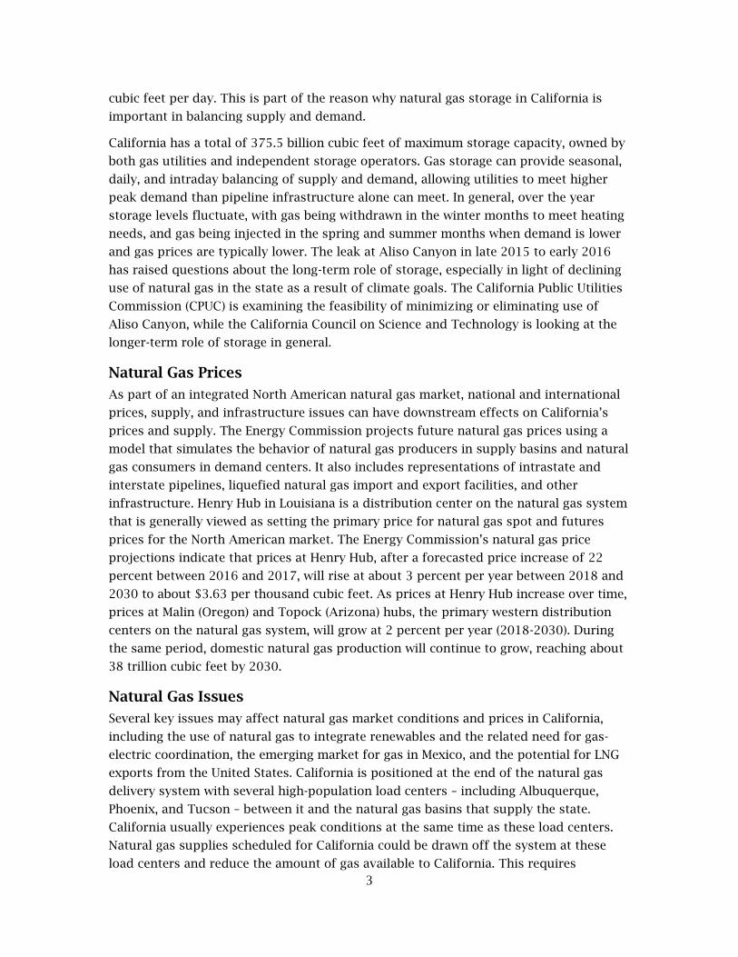
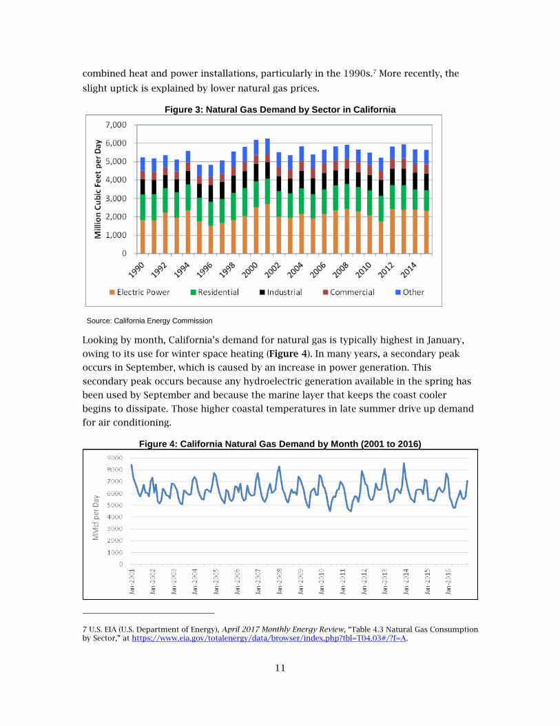
combined heat and power installations, particularly in the 1990s.7 More recently, the

slight uptick is explained by lower natural gas prices.

Figure 3: Natural Gas Demand by Sector in California

Source: California Energy Commission

Looking by month, California’s demand for natural gas is typically highest in January,

owing to its use for winter space heating (Figure 4). In many years, a secondary peak

occurs in September, which is caused by an increase in power generation. This

secondary peak occurs because any hydroelectric generation available in the spring has

been used by September and because the marine layer that keeps the coast cooler

begins to dissipate. Those higher coastal temperatures in late summer drive up demand

for air conditioning.

Figure 4: California Natural Gas Demand by Month (2001 to 2016)

7 U.S. EIA (U.S. Department of Energy), April 2017 Monthly Energy Review, “Table 4.3 Natural Gas Consumption by Sector,” at https://www.eia.gov/totalenergy/data/browser/index.php?tbl=T04.03#/?f=A.

12

Source: U.S. EIA, www.eia.gov

Estimates of future natural gas demand for California comes from the Energy

Commission’s demand forecast, except for demand by the power generator sector,

whose development is described in the following section of this chapter.8 The

preliminary natural gas forecast is published by planning area and shows annual

average growth rates for the 2016 to 2028 period ranging from 0.37 percent to 0.98

percent in the mid demand case. This demand is expected to fall once additional

achievable energy efficiency (AAEE) is incorporated in the revised forecast slated to be

complete later this year.9 The utilities, in the 2016 California Gas Report they produce

every other year, forecast growth rates that are actually negative. This should more

closely match growth rates in the Energy Commission’s demand forecast once the AAEE

is incorporated.10

California’s Natural Gas Demand From Power Generation Westwide Electricity market generation and competition across the West affect electricity imports

and use of natural gas for power generation inside California. The Energy Commission

considers this by simulating electricity production westwide, including California. This

simulation, conducted using the PLEXOS production cost model,11 generates estimates

of all fuels used for power generation sector for the Western Electricity Coordinating

Council (WECC) region, including natural gas, on an economic basis.12 Staff’s WECC-wide

production simulation model dataset covers the years 2017 through 2030 for the three

common cases for the 2017 IEPR and one other case with a higher level of AAEE.13 Table

C-1 in APPENDIX C summarizes these cases.

The PLEXOS electricity supply and demand assumptions for California reflect current

policy mandates, such as the state’s RPS, retirement of once-through-cooling plants, and

8 California Energy Commission, Draft Staff Report: California Energy Demand 2018-2028 Preliminary Forecast, August 2017. http://docketpublic.energy.ca.gov/PublicDocuments/17-IEPR-03/TN220615_20170809T083759_California_Energy_Demand_20182028_Preliminary_Forecast.pdf.

9 AAEE savings are in addition to the committed energy efficiency savings already embedded in the demand forecast. AAEE is the incremental energy savings from the future market potential identified in utility potential studies not included in the baseline demand forecast, but reasonably expected to occur, including future updates of building codes, appliance regulations, and new or expanded IOU or POU energy efficiency programs.

10 2016 California Gas Report, p.5, https://www.pge.com/pipeline_resources/pdf/library/regulatory/downloads/cgr16.pdf.

11 PLEXOS is a modeling platform owned by Energy Exemplar Ltd. Various models of this type are routinely used to estimate electricity production costs and calculate fuel use, as well as hours of operation by the various generators used to produce electricity.

12 The WECC region, also known as the Western Interconnection, extends from Canada to Mexico and includes the provinces of Alberta and British Columbia in Canada; the northern portion of Baja California, Mexico; and all, or portions of, 14 western states in the United States.

13 Additional achievable energy efficiency is savings from initiatives that are planned but not yet approved by the utilities or any other entity.

http://www.eia.gov/

13

Senate Bill 350 energy efficiency targets. Details regarding modeling assumptions are

discussed in APPENDIX C of this report.

Figure 5 highlights the growing dependence on renewables and energy efficiency

resources to meet the forecast of California’s electricity retail sales, while reducing the

need for natural gas, large hydro, and nuclear resources.

Figure 5: California’s Projected Preferred Resources

Source: California Energy Commission, 2017 PLEXOS results

Figure 6 shows natural gas demand for the residential, commercial, and industrial

sectors. California mid case natural gas demand for all three sectors is relatively flat

through the forecast period.

14

Figure 6: California Residential, Commercial, and Industrial Mid Demand Case 2014-2028 (Tcf)

Source: California Energy Commission. California Energy Demand 2018-2028 Preliminary Forecast, August 2017.

Future Electric Generation Natural Gas Demand Figure 7 shows the PLEXOS simulation results for annual California natural gas use for

power generation for all three common cases. A slight expansion in gas used for power

generation in the mid part of the forecast can be attributed partially to the retirement of

the 1,775 MW coal-fired Intermountain Power Plant in Utah and its replacement with a

1,200 MW gas-fired unit. However, the end of the forecast period projects a contraction

due to the increased contribution of renewable resources and AAEE targets.

Figure 7: California Annual Natural Gas Use for Power Generation for All Cases

Source: California Energy Commission, PLEXOS results

Figure 8 shows annual natural gas consumption for electric generation for the WECC

region. WECC-wide, there is an expansion of close to 300 Bcf per year (820 million cubic

feet per day) over the forecast period, or an increase of 13 percent by 2030. This is

0

0.1

0.2

0.3

0.4

0.5

0.6Tr

illio

n C

ub

ic F

ee

t

Total Residential Total Commercial Total Industrial

15

driven largely by the retirement of almost 16,000 MW of coal in the West by 2030 and

the expected replacement with gas-fired generation.

Figure 8: WECC-Wide Annual Natural Gas Use for Power Generation for All Cases


Figure 9 also shows that the natural gas demand for electricity generation in California

decreases, as existing gas-fired generation operates less frequently and at lower load

factors.

Figure 9: California Annual Natural Gas Generation

Source: California Energy Commission, PLEXOS results.

The results for the western United States project that natural gas power generation will

increase by roughly 20 percent, increasing from about 225,000 gigawatt-hours (GWh) in

2016 to about 260,000 GWh in 2028 for the 2017 IEPR mid demand case (Figure 10).

Some of this growth is economic, with natural gas prices projected to remain low so that

gas-fired generation continues to compare favorably to the cost of coal-fired generation

in the near term. Over the long term, the generation growth is driven by retirements of

16

coal generation facilities as power plants end the useful life and power purchase

agreements expire. Many western utilities have indicated plans to replace these aging

coal plants with natural gas-fired power plants. The largest increase in natural gas

generation is between 2024 and 2026, when nearly one-third of the expected coal

retirements are assumed to retire, while 1,200 megawatts (MW) of new natural gas-fired

plants and 4,500 MW of new renewable capacity become operational.14 During this

period, more than 3,000 MW of coal powered plants are also assumed to retire.

The WECC-wide dispatch simulation includes the Canadian provinces of British

Columbia and Alberta. The Alberta Electric System Operator (AESO) has announced

plans to achieve a complete coal phaseout in Alberta by 2030. AESO provides its

reference case scenario for replacing retired capacity with renewables and natural gas

plants in the 2017 AESO Long-term Outlook, which was used as the basis for the model

generation buildout.15

Figure 10: Western United States Annual Natural Gas Generation


Each of the common cases developed in PLEXOS displays an increase in total hours of

gas-fired generation. Comparing the California results with the WECC results in the mid

demand reveals that California’s share of gas-fired generation decreases from 44

percent of the total WECC-wide in 2016 to 33 percent by 2028. These results show

California reducing its reliance on natural gas while the rest of the WECC’s natural gas

generation increases. Similar findings apply to the high and low cases.

14 The Diablo Canyon Power Plant (2,400 MW) is also assumed to retire and, per the proposed settlement, to be replaced with preferred resources.

15 The Alberta Electric System Operator 2017 Long-term Outlook describes Alberta’s expected electricity demand over the next 20 years, as well as the expected generation capacity needed to meet that demand, https://www.aeso.ca/grid/forecasting/.

17

The natural gas demand projections from the PLEXOS modeling for WECC-wide

electricity generation (including California), along with the Energy Commission’s

forecasted demand for the other end uses inside California, become inputs to staff’s

North American Market Gas-trade (NAMGas) model.16 The natural gas demand forecast

assumptions for the rest of the United States come from applying an econometric

analysis state by state to U.S. EIA recorded data by sector. These combined forecasts

give the natural gas demand inputs to NAMGAS.17

16 The NAMGas model simulates the economic behavior of natural gas producers in supply basins and natural gas consumers in demand centers. The model will be described in detail in Chapter 5.

17 NAMGAS solves for demand, supply, and price simultaneously and, as it does so, applies elasticities to come up with final equilibrium demand for all sectors that is different from the demand inputs described in this chapter.

18

CHAPTER 3: Natural Gas Sources and Production

Natural gas produced from underground reservoirs can be either dry or wet gas. Wet gas

contains methane and natural gas liquids such as propane, ethane, and butane, while

dry gas is associated with fewer liquids.18 In the last 20 years, technological innovations

in hydraulic fracturing (sometimes called fracking)19 and horizontal drilling have

allowed for the widespread production of shale-deposited natural gas and other deposit

types. In addition, imports of LNG are used to supplement natural gas supplies mainly

on the East Coast. This chapter discusses natural gas production and LNG imports.

Natural Gas Sources and Production The abundance of shale gas resources increased proved reserves, making the United

States the largest among gas-producing countries in 2011.20 Natural gas production,

climbing since 2005, reached more than 77,000 million cubic feet (MMcf) per day in

2016. Natural gas produced from shale formations drove total production in the United

States to a record high in 2015, and, by 2016, 60 percent of dry natural gas production

originated from this formation type. As of 2015, the latest full year for which data are

available, the United States is still the leading producer of natural gas among gas-

producing countries. Shale formations such as the Marcellus (Pennsylvania, New York,

and West Virginia) and the Utica (Ohio and West Virginia) are producing large quantities

of natural gas. The U.S. EIA estimated that, in 2016, “about 60 percent of total U.S. dry

natural gas production” originated from shale formations.21

Today, most of the natural gas consumed in California originates from the following

out-of-state sources:

Western Canadian Sedimentary Basin (Alberta and British Columbia, Canada)

Permian basin (Texas and New Mexico)

San Juan basin (New Mexico and Colorado)

Rocky Mountain region (Wyoming and surrounding states)

18 Dry gas deposits are natural gas accumulations with less than 0.1 gallons of liquid per thousand cubic feet; wet gas deposits have more than 0.1 gallons of liquid per thousand cubic feet.

19 Hydraulic fracturing involves the pumping of a sand-laden viscous fluid, into a well/wellbore, to create fractures in a rock formation that stimulate the flow of natural gas or oil, increasing the volumes that can be recovered. Wells may be drilled vertically hundreds to thousands of feet below the land surface and may include horizontal or directional sections extending thousands of feet.

20 U.S. EIA, International rankings, https://www.eia.gov/beta/international/.

21 U.S. EIA, Frequently Asked Questions, https://www.eia.gov/tools/faqs/faq.php?id=907&t=8.

19

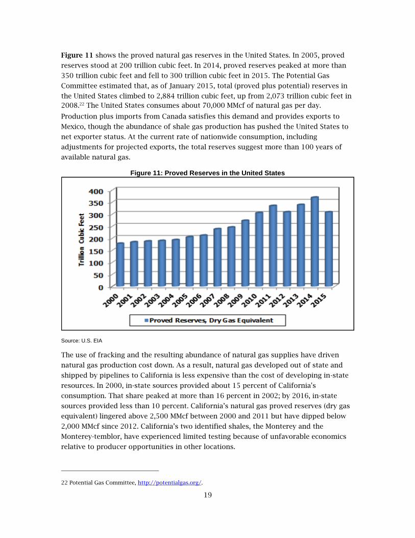
Figure 11 shows the proved natural gas reserves in the United States. In 2005, proved

reserves stood at 200 trillion cubic feet. In 2014, proved reserves peaked at more than

350 trillion cubic feet and fell to 300 trillion cubic feet in 2015. The Potential Gas

Committee estimated that, as of January 2015, total (proved plus potential) reserves in

the United States climbed to 2,884 trillion cubic feet, up from 2,073 trillion cubic feet in

2008.22 The United States consumes about 70,000 MMcf of natural gas per day.

Production plus imports from Canada satisfies this demand and provides exports to

Mexico, though the abundance of shale gas production has pushed the United States to

net exporter status. At the current rate of nationwide consumption, including

adjustments for projected exports, the total reserves suggest more than 100 years of

available natural gas.

Figure 11: Proved Reserves in the United States

Source: U.S. EIA

The use of fracking and the resulting abundance of natural gas supplies have driven

natural gas production cost down. As a result, natural gas developed out of state and

shipped by pipelines to California is less expensive than the cost of developing in-state

resources. In 2000, in-state sources provided about 15 percent of California's

consumption. That share peaked at more than 16 percent in 2002; by 2016, in-state

sources provided less than 10 percent. California’s natural gas proved reserves (dry gas

equivalent) lingered above 2,500 MMcf between 2000 and 2011 but have dipped below

2,000 MMcf since 2012. California’s two identified shales, the Monterey and the

Monterey-temblor, have experienced limited testing because of unfavorable economics

relative to producer opportunities in other locations.

22 Potential Gas Committee, http://potentialgas.org/.

20

In Canada, the resource base consists of 77 trillion cubic feet of proved reserves and

1,087 trillion cubic feet of potential.23 The Canadian oil and gas industry has begun to

use fracking techniques and horizontal drilling that have resulted in expanding

production. The increased production supports the country’s exports to the United

States, including California.

Shale-Deposited Natural Gas Technological innovations in exploration, drilling, and hydraulic fracturing have

transformed shale formations from marginal producers of natural gas to substantial

contributors to the natural gas supply portfolio. In 2007, shale formations produced

about 5,000 MMcf per day, a volume more than eight times the 1998 average of 656

MMcf per day. By 2016, dry gas production averaged more than 43,000 MMcf per day.

Figure 12 displays the average daily dry gas production from shale formations.

Natural gas from shale formations is increasing the associated share of the Lower 48

supply portfolio, growing from about 1 percent in 1998 to more than 50 percent in

2015. As of January 1, 2015, the Potential Gas Committee (PGC) estimates that shale

formations contain about 1,253 Tcf of recoverable natural gas reserves. Figure 12

demonstrates the expansion of shale gas production over the last 16 years.

Figure 12: Average Daily Shale Production (2000-2016)

Source: U.S. EIA.

Hydraulic fracturing and horizontal drilling have decreased the unit cost to find and

develop natural gas reserves. As result, the development of shale-deposited natural gas

surged. The oil and gas industry relies on horizontal wells to access shale formations,

and Figure 13 demonstrates this fact. Since around 2009, the number of vertical wells

drilled (rig count, shown on left axis) has collapsed, while the number of horizontal

wells drilled has expanded and exceeds the number of vertical wells.

23 Canadian Association of Petroleum Producers, www.capp.ca.

21

The industry’s heavy reliance on horizontal wells to access shale formations establishes

a linkage between prices and wells drilled (rig count). Figure 13 shows the relationship

between level of investment (as represented by the horizontal rig count, left axis) and

prices (as represented by Henry Hub spot prices, right axis).

In general, the graph shows that investments rise and fall with prices. Declining prices

usually force cutbacks and postponements in scheduled drilling programs. In August

2008, with prices hovering around $11.00/Mcf, the weekly horizontal rig count climbed

to more than 600. As prices plunged in late 2008 and early 2009, the horizontal rig

count dropped to fewer than 450. The industry experienced a similar phenomenon

between 2014 and 2016. As such, current and expected market prices determine the

level of investments in shale formation drilling and development.

Even though the industry is drilling fewer wells, in general starting around 2012, both

proved and potential natural reserves have continued the upward trajectory. This

trajectory indicates that natural gas recovery per well is increasing.

Figure 13: Horizontal and Vertical Wells Drilled in the United States Versus Natural Gas Prices

Source: Baker Hughes, U.S. EIA.

Environmental Implications of Shale Gas Development While technological innovations have increased the development of natural gas from

shale formations, widespread use of these techniques has raised environmental and

other concerns. First, shale formation development may pose an environmental risk to

the groundwater supply of surrounding communities. Further, the carbon footprint of a

single horizontal well far exceeds that of a typical single vertical well since the drilling

process, completion, and hydraulic fracturing require more carbon-based fuels, drilling

22

mud, and water. Also, running the required equipment and pumps produces more

emissions.

In 2013, the California Legislature passed, and the Governor signed, Senate Bill 4

(Pavley, Chapter 313, Statutes of 2013). In November 2013, the California Department of

Conservation began the formal rulemaking for well stimulation treatment regulations.

As part of SB 4, on July 1, 2015, the Division of Gas and Geothermal Resources (DOGGR)

certified the final environmental impact report, Analysis of Oil and Gas Well Stimulation

Treatments in California. 24 Also under SB 4, on July 9, 2015, the CCST released its final

report on well stimulation, An Independent Scientific Assessment of Well Stimulation in

California.25

As a result, a set of rules and regulations, taking effect in 2014, requires oil and gas well

operators “to submit notification of well stimulation treatments and various types of

data associated with well stimulation operations, including chemical disclosure of well

stimulation fluids, to the Division.”26 In addition, the California Department of

Conservation now compiles submitted information regarding these activities and makes

such information available to the public in a searchable database.

Hydraulic fracturing produces large quantities of wastewater, which field operators

inject into deep wells for disposal. Several jurisdictions, including Ohio, Oklahoma, and

Arkansas, have experienced increased frequency of seismic events (earthquakes > 3.0 on

the Richter scale). The United States Geological Survey (USGS) examined the linkage

between seismicity and wastewater disposal. The agency concluded that “[f]racking is

not causing most of the induced earthquakes. Wastewater disposal is the primary cause

of the recent increase in earthquakes in the central United States.” Further, the USGS

added that “[w]astewater disposal wells typically operate for longer durations and inject

much more fluid than hydraulic fracturing, making them more likely to induce

earthquakes.”27

Given the geologic framework in California, this could be an issue if in-state production

with fracking techniques were developed. The USGS and other institutes and agencies

are continuing work to better understand the linkage between wastewater disposal and

earthquakes. The results of these studies can inform decision-makers about how much

of an impact this issue could have on California’s oil and gas operations.

Liquefied Natural Gas Imports

24 DOGGR, SB 4 Environmental Impact Report,

http://www.conservation.ca.gov/dog/Pages/SB4_Final_EIR_TOC.aspx.

25 CCST, http://ccst.us/projects/hydraulic_fracturing_public/SB4.php.

26 California Department of Conservation, Interim Well Stimulation, http://www.conservation.ca.gov/dog/Pages/WellStimulation-OLD.aspx .

27 U.S. Geological Survey, Earthquake Hazards Program, https://earthquake.usgs.gov/research/induced/myths.php.

http://www.conservation.ca.gov/dog/Pages/SB4_Final_EIR_TOC.aspx

http://ccst.us/projects/hydraulic_fracturing_public/SB4.php

23

In the late 2000s, facing declining production from traditional natural gas supply

basins, the United States considered LNG importation as a way to diversify existing

natural gas supply sources. While the United States still imports and exports LNG, the

lower cost of domestic supplies has reduced the demand for imports. As of May 2017,

operators in the continental United States manage more than 18 Bcf/day of LNG import

capacity – much of it underused. Liquefied natural gas imports enter the United States

mainly through the country’s pipeline system on the Eastern Seaboard. States in the

Northeast, mid-Atlantic, and Southeast are highly populated, and those in the northern

portion of the Eastern Seaboard have cold winters. Moreover, pipeline capacity is

constrained in the Northeast and the Southeast.

While LNG imports have declined from 349 Bcf in 2011 to 88 Bcf in 2016,28 the following

three LNG import facilities account for more than 95 percent of total importations:

Everett LNG in Massachusetts, Cove Point LNG in Maryland, and Elba Island LNG in

Georgia. In 2016, 95 percent of the LNG imported into the United States originated from

Trinidad, located just off the northeast coast of Venezuela. Much of the remaining LNG

imports come from Norway.

LNG on the Pacific Coast While much of the activity related to LNG in the United States is occurring on the

Atlantic and Gulf Coasts, this section discusses LNG activity in Canada’s Pacific Coast,

Oregon, and Baja California, and the relation to the California natural gas market.

Liquefied natural gas activity on the Pacific Coast is relevant to California’s natural gas

market, as proposed LNG export facilities may draw natural gas supply from resource

areas that California already uses, including those in western Canada along with the

Rockies and the Southwest in the United States.

Across the border from California, in Baja California, Mexico, there is the 1 Bcf/day

Costa Azul LNG import terminal in Ensenada, which opened in May 2008 at a cost of $1

billion. Sempra, the parent company of Southern California Gas Co. (SoCalGas) and San

Diego Gas & Electric Company (SDG&E), owns and constructed Costa Azul LNG. Costa

Azul LNG has a berth that could accommodate one LNG tanker ship. Natural gas

received at Costa Azul LNG could be exported to California via pipeline at Otay Mesa in

San Diego or at Ogilby in Imperial County. At Costa Azul, the natural gas is regasified

and distributed to a spur pipeline that connects with the 186-mile-long Gasoducto

Rosarito pipeline in northern Mexico.

In a 2009 presentation,29 Sempra claimed that California consumers having access to

regasified LNG from Costa Azul would be a secure supply source similar to existing gas

production basins in North America (San Juan, Rockies, and western Canada), with the

28 U.S. EIA, U.S. Natural Gas Imports by Point of Entry, https://www.eia.gov/dnav/ng/ng_move_poe1_a_EPG0_IML_Mmcf_a.htm.

29 Sempra LNG Update to the California Energy Commission, August 2009, http://www.energy.ca.gov/lng/documents/costa_azul/2009-08-04_Sempra_LNG_Update_Presentation.pdf.

24

level of supply being determined by market forces. Regarding a Sempra LNG contract

with the Mexican national electric company, Comisión Federal de Electricidad (CFE),

Sempra also stated that LNG delivered from Costa Azul to Mexico will increase natural

gas supply available for delivery to California consumers. Sempra LNG has contractual

commitments to CFE that are being supplied by natural gas delivered from the United

States.

The U.S. EIA’s International Energy Outlook 2016 report succinctly explains the market

conditions at Costa Azul. The report states that imports at the Energía Costa Azul

terminal have averaged only 4 percent of the nameplate capacity of the terminal since

2011. Sempra originally constructed the terminal to supply the Southern California

market and new power plants in Baja California. However, those plants also could be

supplied via pipelines from the United States. In addition, the terminal depended mostly

on natural gas demand in California, which was limited by the availability of less costly

U.S. supplies. The Costa Azul contract allowed for most of the contracted supply from

Indonesia to go instead to higher-priced Asian markets over the past several years.”

Sempra also has an agreement to sell gas from Costa Azul to California utilities. A 2006

comprehensive legal settlement with the State of California to resolve the Continental

Forge litigation included an agreement that, for a period of 18 years beginning in 2011,

Sempra Natural Gas would sell to the California utilities, subject to annual CPUC

approval, up to 500 MMcf/per day of regasified LNG from Sempra Mexico’s Energía

Costa Azul facility that is not delivered or sold in Mexico at the California border index

minus $0.02 per MMBtu. There are no specified minimums required, and to date,

according to Sempra Energy’s 2016 Annual Report,30 Sempra Natural Gas has not been

required to deliver any natural gas under this agreement.

Current economics are pushing Sempra to consider improvements at Costa Azul that

would allow for LNG exports. Specifically, in February 2015, Sempra Natural Gas, IEnova,

and a subsidiary of PEMEX (the state-owned oil company in Mexico) entered into a

memorandum of understanding to develop a natural gas liquefaction project at this LNG

terminal. According to Sempra Energy’s 2016 Annual Report, Sempra Mexico is applying

for the primary governmental authorizations for the project. This project could impact

California, as Costa Azul is connected to pipelines that receive natural gas from the

American Southwest. California also receives gas from this region and could be

competing with a Costa Azul LNG export facility for supplies.

30 Sempra Energy, Balance Growth: 2016 Annual Report, http://www.sempra.com/2016_annualreport/.

http://www.sempra.com/2016_annualreport/

25

CHAPTER 4: Natural Gas Infrastructure

Adequate infrastructure including transmission pipelines, storage, distribution mains,

and related equipment is necessary to safely meet the needs of state’s natural gas

consumers. About 90 percent of California’s natural gas supply is delivered to its

borders through several interstate pipelines that originate in production basins located

several hundred and, in some cases, thousands of miles away. The state’s natural gas

utilities then deliver natural gas to consumers through their distribution systems. In-

state underground storage plays an important role in balancing gas supply and demand

on the system, especially during periods of high demand. The state’s gas utilities are

addressing safety and environmental concerns on their gas systems by replacing and

upgrading aging infrastructure. Issues related to interstate and in-state natural gas

infrastructure are discussed in this chapter.

Interstate Natural Gas Pipelines The natural gas pipeline network in the United States consists of an integrated

transmission and distribution system that transports natural gas from numerous

producing basins to users all over the country via 318,000 miles of interstate and

intrastate transmission lines.31 The pipeline systems of Canada and Mexico connect to

this system so that natural gas can flow between the three countries. These interstate

pipelines deliver natural gas to the California border, where it enters the in-state gas

system operated primarily by California’s gas utilities. Some large natural gas users,

mostly power plants, receive their gas directly from interstate pipelines.

Figure 14 shows the pipelines and production basins that supply gas to California.

These interstate pipelines provide California with supplies from the U.S. Southwest,

Rocky Mountains, and western Canada, and regasified LNG, as discussed in Chapter 3.32

The maximum delivery capacities of these pipelines that serve California, as shown in

31 U.S. Department of Transportation Pipeline and Hazardous Materials Safety Administration (PHMSA) PHMSA, https://www.phmsa.dot.gov/pipeline/library/data-stats.

32 SoCalGas, 2016 California Gas Report, prepared by California's gas and electric utilities, p.4 https://www.socalgas.com/regulatory/documents/cgr/2016-cgr.pdf.

26

Table 1, provide a total maximum delivery capacity of up to 12.89 Bcf/day. However,

California’s capacity to receive gas from those pipelines is only about 9 Bcf/day.33 This

exceeds the state's average consumption of about 6 Bcf/day but is less than California’s

recorded peak-day consumption of 11.157 Bcf, which occurred on December 9, 2013.34

Figure 14: Western North American Natural Gas Pipelines

33 Staff estimated this using data from the 2016 California Gas Report.

34 SoCalGas, 2016 California Gas Report, p. 29.

27

Source: 2016 California Gas Report, https://www.socalgas.com/regulatory/cgr.shtml

Western North American Natural Gas Pipelines Legend

1. El Paso Natural Gas 13. Southern California Gas Company

2. Gasoducto Bajanorte (GB) 14. Transportadora de Gas Natural (TGN)

3 Gas Transmission Northwest (GTN) 15. TransCanada Pipeline

4. Kern River Pipeline 16. Transwestern Pipeline

5. Mojave Pipeline 17. Tuscarora Pipeline

6. North Baja Pipeline 18. Unused

7. Northwest Pipeline 19. Ruby Pipeline

8. Piute Pipeline 20. Kern River Expansion

9. Pacific Gas & Electric Company 21. Sunstone Pipeline

10. Questar Southern Trail Pipeline 22. Transcolorado Pipeline

11. Rockies Express 23. Pacific Connector Pipeline

12. San Diego Gas & Electric Company

https://www.socalgas.com/regulatory/cgr.shtml

28

Table 2 provides information on the quantities of natural gas shipped to California

along main interstate pipeline systems. The maximum capacities reported in

29

Table 1 do not equate to actual deliverability. According to the 2016 California Gas

Report, SoCalGas could receive up to 3,875 MMcf/day in firm capacity from interstate

pipelines, while Southern California’s upstream capacity is 6,765 MMcf/day.35 For

example, while the physical interconnection that PG&E has with SoCalGas at Kern River

has a physical capacity of 650 MMcf/day, PG&E could deliver only up to 520 MMcf/day

from that interconnection point to SoCalGas. North Baja, for example, is not designed to

“serve” California but rather transports gas through California from Ehrenberg, Arizona,

into Mexico’s Baja Norte system.36 The combined physical capacity of both Gas

Transmission Northwest (GTN) and the Ruby pipelines, which deliver natural gas to

Malin, Oregon, totals 3,956 MMcf/day. PG&E’s Redwood Path (Lines 400/401) is

connected to GTN, and Ruby has a firm capacity of only 2,023 MMcf/day.37 These

differences in interstate pipeline capacity and in-state pipeline capacity explain why

California does not fully use the capacity of interstate pipeline systems delivering gas to

the state.

35 Pg. 81-82, 2016 California Gas Report.

36 Pg. A-1, California Energy Commission, AB 1257 Natural Gas Act Report: Strategies to Maximize the Benefits

Obtained from Natural Gas as an Energy Source.

37 Pg. 41, 2016 California Gas Report.

30

Table 1: Main Interstate Pipeline Systems Serving California (Bcf/day)

Pipeline System

Maximum

Capacity

Average Capacity Utilization Rates

(2012-2016)

Gas Transmission

Northwest (GTN) 2.272 51%

Ruby 1.684 46%

Kern River 1.942 77%

El Paso North 2.033 35%*

El Paso South 1.459 35%*

Transwestern 1.150 65%

Mojave 0.976 19%

Southern Trails 0.120

Incorporated into Other in the 2017

California Gas Report Supplement

TGN 0.415

Utilization not reported in the 2017


Tuscarora Gas

Transmission Company 0.236

Utilization not reported in the 2017


North Baja Pipeline System 0.600

Not designed to “serve” California but

transports gas from Arizona through

California to serve Mexico.

Total 12.89

Sources: PointLogic, 2017 Supplemental California Gas Report, https://www.socalgas.com/regulatory/cgr.shtml

*Average capacity utilization rate for both El Paso North and South combined.

31

Table 2: Utilization of Main Interstate Pipeline Systems (Bcf/day)

Year El Paso Transwestern GTN Kern

River

Mojave Other* Ruby Total

2012 1.081 0.865 1.064 1.814 0.396 0.046 0.872 6.138

2013 1.181 0.945 0.948 1.429 0.161 0.109 0.779 5.552

2014 1.155 0.832 1.173 1.414 0.23 0.084 0.826 5.714

2015 1.544 0.491 1.26 1.251 0.111 0.413 0.758 5.828

2016 1.104 0.611 1.331 1.543 0.014 0.128 0.631 5.362

Source: 2017 Supplemental California Gas Report, https://www.socalgas.com/regulatory/cgr.shtml.

*The 2017 Supplemental California Gas Report reports El Paso North and El Paso South as one.

**Includes storage activities, volumes delivered on Questar Southern Trails for SoCalGas and PG&E.

Natural Gas Storage Facilities in California Underground natural gas storage plays an important role in balancing California’s

demand requirements with supply availability. California has 14 natural gas storage

facilities: four owned by SoCalGas, three by PG&E, and seven by independent operators.

Table 3 shows the natural gas storage working capacity in California. The table also

breaks down natural gas storage in California by utility-owned and independently

owned working capacity. Natural gas storage facilities (including independently owned)

that are interconnected to PG&E’s natural gas system have a working gas capacity of

240.2 Bcf. SoCalGas operates four storage fields that interconnect with its transmission

system and have a working gas capacity totaling 135.3 Bcf. Combined, the systems of

both gas utilities have a capacity of 375.5 Bcf.

32

Table 3: California Natural Gas Storage Working Capacity

Working

Capacity(Bcf)

Maximum

Withdrawal

Capacity(Bcfd)

California 375.5

Utility-owned

& Controlled

PG&E 38 102.2 1.5

SoCalGas 135.3 3.7

Independently-

owned

138.0 2.9

Sources: U.S. EIA Natural Gas Annual Respondent Query System (EIA-191 Data through

2015),https://www.eia.gov/cfapps/ngqs/ngqs.cfm?f_report=RP7&f_sortby=&f_items=&f_year_st

art=&f_year_end=&f_show_compid=&f_fullscreen.

As the discussion of interstate pipeline capacity above indicates, pipeline flows into the

state at the receipt points at the border, which are less than the interstate pipelines can

deliver, are not sufficient to meet peak demand. In general, gas storage can provide

seasonal, daily, and intraday balancing of supply and demand, allowing utilities to meet

higher peak demand than pipeline infrastructure might otherwise allow.

Table 4 includes aggregated, or combined, data of injections and withdrawals of

California natural gas storage facilities.39

Table 4: Injections and Withdrawals at California Natural Gas Storage Facilities MMcf

2011 2012 2013 2014 2015 2016

Injections 263,067 218,663 182,046 280,516 206,774 124,474

Withdrawals 242,477 170,586 268,548 235,181 204,077 164,077

Net

Withdrawals

-20,590 -48,077 86,502 -45,335 -2,697 39,603

Source: U.S. EIA

Within the calendar year, storage levels fluctuate as natural gas withdrawal figures are

higher during the winter months to meet heating demand, while injections are higher in

38 California Energy Commission, Natural Gas Market Assessment, Staff Report , 2003, p. 51, http://www.energy.ca.gov/reports/2003-08-08_100-03-006.PDF. Accessed July 2017.

39 The reduced availability of Aliso Canyon is reflected in the decline in natural gas injections and withdrawals between 2015 and 2016.

33

the spring and summer as space heating demand declines in those months, as shown in

Figure 15.

Figure 15: Natural Gas Storage Levels by Month for California Natural Gas Storage Facilities

Source: U.S. EIA

November is when California’s natural gas storage levels are at their annual peak, just

before the winter withdrawals.

34

Figure 16 shows November storage levels for California natural gas storage facilities for

the years 2001 through 2016. As with injections and withdrawals, the low November

storage level is low due to the loss of Aliso Canyon.

35

Figure 16: November Storage Levels for California Natural Gas Storage Facilities (2001-2016)

Source: California Energy Commission, using PG&E and SoCal gas data

Long-Term Role of Storage The long-term role of storage in California’s gas system has been brought into question

as a result of the methane leak at Aliso Canyon that occurred in late 2015 and early

2016. On July 19, 2017, following months of testing, inspection, and implementing new

safety protocols, DOGGR and the CPUC concurred that the facility is safe to operate at a

greatly reduced capacity and with restrictions on withdrawing gas only if there is a

reliability issue. The Energy Commission’s 2017 IEPR includes a chapter on energy

reliability issues in Southern California. That chapter details the energy reliability

impacts of the Aliso Canyon leak, along with information on mitigation measures.

Also on July 19, 2017, Energy Commission Chair Robert B. Weisenmiller released a letter

to CPUC President Michael Picker urging the CPUC to plan for the future closure of the

Aliso Canyon natural gas storage facility. In that letter, Chair Weisenmiller wrote that

Energy Commission staff is prepared to work with the CPUC and other agencies on a

plan to phase out the use of the Aliso Canyon natural gas storage facility within 10

years.40

Senate Bill 380 also required the CPUC to open a proceeding to determine the feasibility

of minimizing or eliminating the use of SoCalGas’s Aliso Canyon storage facility while

maintaining energy and electric reliability for the Los Angeles region. In response, the

CPUC opened a proceeding (called an order instituting investigation; I.17-02-002) and

expects to make a final decision in this proceeding in mid-2018.

40 California Energy Commission, News Release: "Energy Commission Chair Releases Letter Urging the Future Closure of Aliso Canyon," July 2017.

36

Finally, the California Council on Science and Technology (CCST) is developing a report

that will include a review of potential health risks and community impacts associated

with the operation of Aliso Canyon; fugitive gas emissions; and the linkages between gas

storage, California's current and future energy needs, and its GHG reduction goals. 41

Staff expects this report to be completed by late December 2017.

Natural Gas Pipeline Safety Natural gas infrastructure safety has become more prominent since the explosion of a

PG&E high-pressure pipeline in San Bruno in September 2010 and the major gas leak at

Aliso Canyon. With the aim of addressing natural gas infrastructure safety in the wake

of these events, the CPUC has authorized increased revenue requirements for Pacific

Gas and Electric (PG&E), Southern California Gas (SoCalGas), and San Diego Gas and

Electric (SDG&E) related to transmission and distribution. As gas utilities place greater

emphasis on safety and replacing aging infrastructure, natural gas utility revenue

requirements for transmission, distribution and storage services increased by 11.9

percent in 2016, 12.6 percent in 2015, and by 45 percent from 2010 until 2017.42 Table

5 shows that the increases in total authorized revenue requirements for transmission,

distribution, storage, and customer services, combined under the “transportation”

category, have increased by 73 percent from 2011 to 2016.43 Such costs increased by

115, 45, and 48 percent for PG&E, SoCalGas, and SDG&E, respectively, from 2011 to

2016.

Table 5: Historical Revenue Requirements for Transportation Summary ($000)

Utility 2011 2012 2013 2014 2015 2016

PG&E $1,533,332 $1,731,021 $1,828,380 $2,076,507 $2,500,926 $3,292,033

SoCalGas $1,971,438 $2,018,108 $2,218,229 $2,392,986 $2,511,953 $2,850,150

SDG&E $276,573 $244,973 $324,022 $318,647 $378,037 $408,148

Total $3,781,343 $3,994,102 $4,370,631 $4,788,140 $5,390,916 $6,550,331

Source: CPUC Energy Division, California Electric and Gas Utility Cost Report, April 2017.

In its most recent rate case, SoCalGas/SDGE received CPUC approval for funding for

2016 through 2018 for safety enhancements. PG&E’s approval extended from 2017 to

41 CCST, Current Projects: Natural Gas Storage, http://ccst.us/projects/natural_gas_storage/index.php.

42 CPUC, Energy Division, California Electric and Gas Utility Cost Report, April 2017, http://www.cpuc.ca.gov/uploadedFiles/CPUCWebsite/Content/About_Us/Organization/Divisions/Office_of_Governmental_Affairs/Legislation/2017/AB67_Leg_Report_PDF_Final_5-5-17.pdf.

43 CPUC, California Electric and Gas Utility Cost Report, April 2017, p. 41, http://www.cpuc.ca.gov/uploadedFiles/CPUCWebsite/Content/About_Us/Organization/Divisions/Office_of_Governmental_Affairs/Legislation/2017/AB67_Leg_Report_PDF_Final_5-5-17.pdf.

37

2019.44 With this funding, PG&E and SoCalGas/SDG&E will enhance the safety of their

respective pipeline systems by replacing infrastructure, installing cathodic protection to

protect pipelines from corrosion, and performing assessments of their pipeline

systems.45

SoCalGas’s five-year capital plan includes $6 billion in infrastructure investments,

including about $1.2 billion in 2017 for improvements to distribution, transmission, and

storage systems and for pipeline safety.46 In 2017, the CPUC authorized a $58 million

increase from $375 million to $433 million in revenue requirements for the operation

and maintenance of PG&E’s gas distribution system.47

44 General rate cases are proceedings used to address the costs of operating and maintaining the utility system and the allocation of those costs among customer classes. For more information: http://www.cpuc.ca.gov/General.aspx?id=10431.

45 Cathodic protection systems help prevent corrosion from occurring on pipeline exteriors by imparting a direct current onto the buried pipeline using a device called a rectifier. As long as the current is sufficient, corrosion is prevented or at least mitigated and held in check. For more information, please view the PHMSA website at https://primis.phmsa.dot.gov/comm/FactSheets/FSCathodicProtection.htm.

46 SoCalGas, News Release: "SoCalGas Begins a More than $14 Million Pipeline Safety Project in the Counties of San Luis Obispo and Santa Barbara," https://www.socalgas.com/1443740785750/5-25-17-SoCalGas-to-Begin-Infrastructure-Testing-Upgrades-in-SLO-County.pdf.

47 CPUC, Decision 16-06-056: Decision Authorizing Pacific Gas And Electric Company's Revenue Requirement For Gas Transmission and Storage Services and Adopting Interim Rates, http://docs.cpuc.ca.gov/PublishedDocs/Published/G000/M164/K610/164610296.pdf.

38

CHAPTER 5: Natural Gas Prices

As mentioned, California’s natural gas system interconnects with the larger North

American natural gas pipeline network. Because California connects to a natural gas

pipeline network that encompasses North America, staff modeled supply, demand, the

transportation of natural gas, and its production in North America. Natural gas prices

are set in competitive markets nationwide with some differences in regional

submarkets.

Energy Commission staff uses the NAMGas model to simulate the economic behavior of

natural gas producers in supply basins and natural gas consumers in demand centers.

The model also includes representations of intrastate and interstate pipelines, LNG

import and export facilities, and other infrastructure.

The model encompasses the regions of the continental United States, Alaska, Canada,

and Mexico. Staff developed three “common” cases for the 2017 IEPR: the high demand,

mid demand, and low demand cases, using inputs and assumptions such as increased

energy efficiency and renewable generation and varying amounts of coal-fired electrical

generation retirements. The inputs and assumptions are expected to have an impact on

the natural gas market. In addition, values for proved and potential reserves in North

America appear on the supply side of the NAMGas model.

In the NAMGas model, producers, consumers, and natural gas transporters try to

maximize economic utility. Suppliers aim to maximize profits while consumers try to

get the lowest price. The model reconstructs the North American natural gas market by

modeling the connections of the North American supply basins to intrastate and

interstate pipelines, which deliver natural gas to demand centers. The model used by

staff was constructed and used over several years.48

For the 2017 Natural Gas Outlook Report, staff updated the model to include North

American natural gas infrastructure, including new pipelines and new LNG export

capacity, while resetting assumptions in the California portion of the model to account

for 2017 IEPR cases. To calibrate the model, actual production and demand data were

used for the years 2014 to 2016, provided by the U.S. EIA, Mexico’s Ministry of Energy,

and Canada’s National Energy Board. The model iterates back and forth among the

aforementioned components to find economic equilibrium at all modeled nodes, which

represented geographic locations. As a consequence, the model produces forecasts of

natural gas supply, demand, and prices.

48 Brathwaite, Leon, Anthony Dixon, Jorge Gonzales, Chris Marxen, Peter Puglia, and Angela Tanghetti. 2015 Natural Gas Outlook Draft Staff Report, California Energy Commission. CEC-200-2015-007-SD, p. 12. Kennedy, Robert, Silas Bauer, Leon Brathwaite, Peter Puglia, Jorge Gonzales, and Katherine Anderson, Natural Gas Issues, Trends, and Outlook Draft Staff Report, 2014, California Energy Commission. CEC-200-2014-001-SD, p. 19.

39

Three “Common” Cases: High Demand, Mid Demand, and Low Demand The variables and assumptions for each of the three common cases are explained in

APPENDIX A. The model incorporates information from the Energy Commission’s

preliminary 2017 California Energy Demand forecast of natural gas for residential,

commercial, industrial, and transportation sectors. The 2015 estimates of California

additional achievable energy efficiency (AAEE) came from the 2015 California Energy

Demand Report.

NAMGas incorporates a forecast of natural gas demand for power plants in the WECC

region. This forecast comes from an electricity dispatch model that uses the PLEXOS

software, incorporating the Energy Commission’s electricity demand forecast as an

input. Staff incorporated August 2017 PLEXOS model run outputs into the NAMGas

model as well as estimates of coal retirements WECC-wide through the year 2050.

Staff also constructed three common residential, commercial, and industrial natural gas

demand cases for North American regions outside of California and for natural gas

power generation demand outside of the WECC region. To build reference demand for

the three common cases, staff used an econometric model49 that forecasts reference

demand in the residential, commercial, industrial, and transportation sectors outside

California along with natural gas demand for the power generation sector outside the

WECC region. This econometric model, known as “small-m,” includes factors such as

economic growth, an estimate of coal retirements, heating and cooling degree-days,50

and historical demand for natural gas by sector.

Modeling Natural Gas Supply The NAMGas model was populated with assumptions of natural gas supply. The sum of

the proved and potential natural gas reserves defines the natural gas resource base. Two

factors distinguish proved reserves from potential reserves: capital needed for

production and level of certainty of production. Proved reserves comprise all resources

with sufficient geological and engineering information, indicating with reasonable

certainty, that oil and gas operators can recover such reserves using existing technology

under existing economic and operating conditions. Production of proved resources

requires the expenditure of operating and maintenance funds and minimal capital

dollars.

49 An econometric model specifies the hypothesized statistical relationship between the various economic quantities pertaining to a particular economic phenomenon under study. Staff’s small “m” model uses variables including economic growth, an estimate of coal retirements, heating and cooling degree days, and historical natural gas demand to build high demand, mid demand, and low demand reference cases for use in the NAMGas model.

50 Heating degree days are a measure of how cold the temperature was on a given day or over a period of

days. Cooling degree days (CDD) measure how hot the temperature was on a given day or over a period of days. See U.S. EIA website: https://www.eia.gov/Energyexplained/index.cfm?page=about_degree_days.

https://www.eia.gov/Energyexplained/index.cfm?page=about_degree_days

40

Potential reserves include all undeveloped resources in the future. Estimates of potential

reserves, published by the PGC’s Potential Supply of Natural Gas in the United States:

Report of the Potential Gas Committee (December 31, 2014),51 provide the basis of

natural gas supply in North America. The model’s computations begin with estimates of

these reserves values.

These resources, geologically known but with decreasing levels of certainty, require

operating and maintenance costs and the full expenditures of capital dollars for the

production of these resources. As total demand for natural gas grows, producers will

bring more of these resources on-line, beginning with the lowest-cost resources. Because

California imports about 90 percent of its natural gas supply from out of state,

estimates of potential and proved reserves of natural gas basins in the United States and

Canada are important components of the NAMGas model.

While the NAMGas model produced hub price backcasts52 and forecasts for natural gas

hubs throughout North America, this paper presents forecasts for the following three

hubs: Henry Hub near Erath, Louisiana, Malin, Oregon; and Topock, Arizona. Henry Hub

serves as the benchmark for natural gas prices in North America while also serving as

the trading location used to price the New York Mercantile Exchange natural gas futures

contracts. Malin, Oregon is the point at which gas enters Northern California from

Canada and the Rocky Mountains. In addition, the Kern River Gas Transmission pipeline

can transport natural gas from the Rocky Mountains to Southern California to

Bakersfield via Daggett, California. Natural gas from both the San Juan Basin in the Four

Corners area and the Permian Basin in western Texas and eastern New Mexico may be

transported to Topock, Arizona.

The Natural Gas Market in the United States (2014-2016) To calibrate the model, staff incorporated historical data from 2014 to 2016. At Henry

Hub, Malin, and Topock, natural gas prices decreased each year from 2014 to 2016. This

is the result of a decade of increased supply in the natural gas market, pushing prices

down. Each year, from 2005 through 2015, dry natural gas production in the United

States increased.

However, dry production in the United States decreased to an estimated 26.46 Tcf in

2016. As prices drop, there will be less economic incentive for producers to invest

capital to develop additional gas wells and to increase production. Available data

reflects this trend. According to the U.S. EIA, the number of producing gas wells in the

United States decreased from nearly 578,000 in 2012 to about 555,000 in 2015.

51 Potential Gas Committee, http://potentialgas.org/biennial-report.

52 A backcast calibrates a model used for forecasting and assesses the model’s ability to produce known results, such as prices in prior years (2014-2016 in the current modeling work). This process should provide results that are close or at the actual prices for 2014, 2015, and 2016.

http://potentialgas.org/biennial-report

41

Nationwide demand for natural gas also increased from 22.91 Tcf in 2009 to 27.49 Tcf

in 2016. This increase is in response to the lower prices that resulted from increased

supplies. Demand growth was strong in the electric generation sector. In the United

States, natural gas demand in the electric generation system increased from 7.57 Tcf in

2011, to an estimated 9.98 Tcf in 2016.

As natural gas prices have declined due to increased production in the United States,

California natural gas utility ratepayers have experienced lower procurement costs. For

example, natural gas procurement costs for core customers for PG&E, SoCalGas, and

SDG&E decreased from $3.55 billion in 2014, to $2.05 billion in 2016 (a 42 percent

decline).53 This trend started in 2010, as natural gas procurement costs fell 51 percent

between 2010 and 2016.54

Natural Gas Price Projections The model provides projections of prices and supply of natural gas for California and

the continental United States for 2017 through 2030. Between 2016 and 2017, natural

gas prices at Henry Hub increased. The daily average Henry Hub price from January 4,

2016, through August 18, 2016, was $2.29/Mcf, 55 while the daily average Henry Hub

price from January 3, 2017, through August 18, 2017, was $3.10/Mcf, an increase of 36

percent.

In the mid demand forecast, the model estimates that the Henry Hub price for 2017 will

be $3.11/Mcf. After a forecasted average price increase of 6.16 percent a year from 2017

through 2020, prices will rise at about 2.06 percent per year between 2020 and 2030.

Staff calculated that after accounting for inflation, prices dropped an average of 6.7

percent per year between 2010 through 2016. The development of shale-deposited

natural gas accounts for the lowering of real prices.56

The faster growth rate in Henry Hub prices occurring from 2017 to 2020 arises from the

substantial development of potential natural gas resources in the United States,

including the Gulf of Mexico, Ohio, and Pennsylvania. The development of these

resources is meeting growing natural gas demand, particularly in the electricity sector in

parts of the South and the latter two states. It is more expensive to produce gas from

potential resource areas as developing those resources requires an upfront investment.

On the other hand, for proved resources, the model assumes that only operation and

maintenance costs (along with minimal capital dollars) are incurred because the major

capital expenditures have already been invested. In addition to the development of new

53 CPUC Energy Division, 2017 California Electric and Gas Utility Cost Report, p. 38, April 2016.

54 CPUC Energy Division, 2017 California Electric and Gas Utility Cost Report, p. 39, April 2016.

55 Hub prices in this chapter are presented in 2016 U.S. dollars.

56 Inflation adjusted.

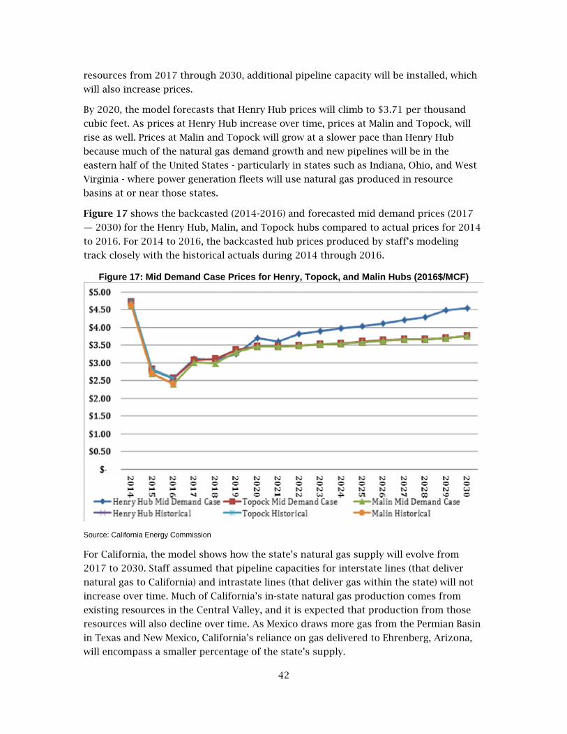
42

resources from 2017 through 2030, additional pipeline capacity will be installed, which

will also increase prices.

By 2020, the model forecasts that Henry Hub prices will climb to $3.71 per thousand

cubic feet. As prices at Henry Hub increase over time, prices at Malin and Topock, will

rise as well. Prices at Malin and Topock will grow at a slower pace than Henry Hub

because much of the natural gas demand growth and new pipelines will be in the

eastern half of the United States - particularly in states such as Indiana, Ohio, and West

Virginia - where power generation fleets will use natural gas produced in resource

basins at or near those states.

Figure 17 shows the backcasted (2014-2016) and forecasted mid demand prices (2017

— 2030) for the Henry Hub, Malin, and Topock hubs compared to actual prices for 2014

to 2016. For 2014 to 2016, the backcasted hub prices produced by staff’s modeling

track closely with the historical actuals during 2014 through 2016.

Figure 17: Mid Demand Case Prices for Henry, Topock, and Malin Hubs (2016$/MCF)


For California, the model shows how the state’s natural gas supply will evolve from

2017 to 2030. Staff assumed that pipeline capacities for interstate lines (that deliver

natural gas to California) and intrastate lines (that deliver gas within the state) will not

increase over time. Much of California’s in-state natural gas production comes from

existing resources in the Central Valley, and it is expected that production from those

resources will also decline over time. As Mexico draws more gas from the Permian Basin

in Texas and New Mexico, California’s reliance on gas delivered to Ehrenberg, Arizona,

will encompass a smaller percentage of the state’s supply.

43

Much of the natural gas delivered to Ehrenberg is produced in the Permian Basin. Staff’s

modeling shows that future deliveries to Ehrenberg will be smaller than in previous

years. While California will rely less on Permian gas, modeling shows that California will

import more natural gas from the San Juan Basin. In the mid demand case, pipeline

exports from the United States to Mexico are forecasted to remain between 1.3 Tcf to

1.5 Tcf per year through 2030. According to the U.S. EIA, pipeline exports to Mexico

from the United States increased from 0.499 Tcf in 2011 to 1.38 Tcf in 2016.

However, the forecast shows the percentage of gas received at Malin, Oregon, to remain

roughly the same at 39 percent of California’s out-of-state supply in 2030, compared to

38 percent in 2016. PG&E’s Redwood Path (Lines 400/401), which is connected to the

Gas Transmission Northwest pipeline and the Ruby pipeline at Malin, Oregon, tends to

operate close to maximum capacity. Modeling results indicate that this will continue.

Furthermore, natural gas received at Malin comes from either Canada or the Rocky

Mountains and will not be used to meet Mexico demand due to the long transport

distance.

It is expected that the United States will export increasing amounts of LNG. In 2016, the

United States exported nearly 187 Bcf of LNG, an all-time high. According to the U.S. EIA,

that amount could increase to 2.4 Tcf to 8.5 Tcf by 2030. Due to the increase in LNG

exports and pipeline exports to Mexico, modeling shows that the United States will be a

net natural gas exporter from 2018 through 2030. While LNG exports will increase,

natural gas production will be sufficient to meet domestic and international demand.

Moreover, the basins that provide natural gas for LNG export in the United States are

not ones that serve California. However, there are proposed pipeline projects that aim to

ship gas from the Permian Basin to LNG export facilities on the Gulf Coast.57 While a

future pipeline from the Permian Basin to the Gulf of Mexico would require California to

compete for supplies with countries that receive U.S. LNG, California is already

forecasted to receive smaller quantities of natural gas from the Permian Basin. Figure

18 shows the forecasted Henry Hub prices for the low demand, mid demand, and high

demand cases. The mid demand case represents a “business-as-usual” environment.

However, the high demand and low demand cases use modified assumptions to the mid

demand case that either push natural demand higher or lower. The high demand case

assumes lower costs for developing proved and potential resources than in the mid

demand case, while the low demand case assumes higher costs than in the mid demand

case.

Furthermore, the high demand case assumes larger estimates of available potential

resources when compared to the mid demand case. Similarly, the low demand case

assumes smaller estimates of potential resources. The additional production in the

57 Natural Gas Intelligence, Kinder Proposing Permian-to-Gulf Coast NatGas Pipeline, March 22, 2017, http://www.naturalgasintel.com/articles/109850-kinder-proposing-permian-to-gulf-coast-natgas-pipeline.

44

higher demand case will result in lower prices during the forecast period while the high

production costs in the low demand case will keep prices high.

Figure 18: IEPR Common Cases for Henry Hub Pricing Point (2016$/MCF)


As the high demand case is also a low-cost case with higher estimates of potential

reserves, production is forecasted to be higher than the mid demand and low demand

cases (Figure 19). U.S. natural gas production in the mid demand case is forecasted to

reach 38 Tcf in 2030, while climbing to 41 Tcf in the high demand case and falling to 28

Tcf in the low demand case. According to the U.S. EIA, dry natural gas production was

26.46 Tcf in 2016.

Figure 19: Natural Gas Production in the United States (Tcf/Year)


Prices from the Energy Commission’s mid demand forecast for the years 2017 through

2030 have declined substantially since the 2011 Natural Gas Market Assessment (Figure

45

20). In 2011, the Energy Commission’s modeling forecasted that the mid demand Henry

Hub price in 2020 would be $6.25/Mcf. In 2015, this estimate fell to $4.27 for 2020.

However, in 2017, the mid demand Henry Hub 2020 price reached only $3.71/Mcf.

Increasing estimates of potential natural gas resources account for the changes seen in

the forecast. Resource estimates are one of the main drivers in the model.

Under each biennial assessment of natural gas resources since 2006, the PGC58 has

increased its estimates of potential resources. The PGC estimated that in 2006, there

were 1,321 Tcf of potential natural gas resources.59 In 2016, the PGC’s estimate has

more than doubled to 2,817 Tcf.60 Much of the additional potential natural gas resources

come from upward revisions of estimates of available natural gas in the Appalachian

Mountains.

Inputs to the NAMGas model include estimates of potential natural gas resources, and

as more natural gas resources can be developed at no change in costs, per unit costs

decline. The reduced costs faced by natural gas producers are passed on in the form of

lower natural gas hub prices.

Figure 20: Energy Commission Forecasted, Actual, and Futures Prices for Henry Hub 2016$/Mcf


58 Housed at the Colorado School of Mines (Boulder, Colorado), the Potential Gas Committee assesses the future supply of natural gas in the U.S and publishes its assessment every two years.

59 Potential Gas Committee, Potential Supply of Natural gas In the United States, p. 3, April 2015.

60 Potential Gas Committee, Press Release: “U.S. Potential Gas Committee Reports Record Future Supply of Natural Gas in the U.S.,” July 19, 2017.

47

CHAPTER 6: Natural Gas Issues

This chapter highlights key issues and trends affecting the outlook for natural gas

market conditions and prices in California. These include the impact of more renewable

energy on natural gas demand, which is one of the factors increasing the need for gas-

electric coordination, the fact that California sits at the western and southern end of the

natural gas pipeline system, the changing market for natural gas in Mexico, and the

prospect of LNG exports.

Renewables and Gas Electric Coordination California's RPS goal now requires 50 percent of the state’s power to be generated by

renewable energy sources by 2030. The California Independent System Operator’s

(California ISO) often shows renewable generation in excess of 30 percent of net

demand.61 It is commonly asserted that natural gas is needed to back up intermittent

renewables, although as prices of demand response and battery storage of electricity

continue to fall, and with the expansion of the regional Energy Imbalance Market, those

resources may be better suited to fill this role. The key impact of renewable energy

intermittency is that natural gas-fired generators will need to ramp up and down

(sometimes quickly and unexpectedly) to fill in behind those renewable resources.

The need to coordinate more between the gas and electricity sectors arises because the

way customers use natural gas is changing, in particular the need to integrate increasing

levels of renewable resources. The electricity market is scheduled on an hourly basis

with some hours having increasingly large swings in gas-fired generation. The tariffs

and operating characteristics of the gas system, however, are predicated on flat hourly

nominations. Until enough energy storage is installed so that renewable generation can

continue to serve load even when it cannot produce electricity, electricity dispatchers

will continue to rely on the natural gas generation fleet to serve electricity demand when

renewable resources are not available.

Nationwide, the percentage of natural gas supply devoted to generating electricity has

doubled over the last 20 years.62 In 2015, natural gas generated almost as many

gigawatts of electricity as coal, and in summer 2016 EIA also reported the first ever net

withdrawal from underground gas storage during a summer month.63, 64 As discussed in

Chapter 2, California’s use of gas for electricity generation varies seasonal and monthly

61 See http://www.caiso.com/Pages/TodaysOutlook.aspx#Power%20Mix%20by%20Fuel%20Type.

62 EIA, Natural Gas Consumption by Year at https://www.eia.gov/dnav/ng/ng_cons_sum_dcu_nus_a.htm.

63 EIA, Total Electric Power Industry Summary Statistics, 2015 and 2014. Found at https://www.eia.gov/electricity/annual/html/epa_01_01.html.

64 U.S. EIA, Today in Energy, August 8, 2016, https://www.eia.gov/todayinenergy/detail.php?id=27412.

48

largely in response to wet versus dry years affecting hydroelectric generation. However,

the RPS and energy efficiency should cause a decrease in the gigawatt hours of

electricity generated with natural gas by 2028. It is incidents such as the 2011 cold

weather event that caused gas curtailments to electric generators in San Diego and the

constrained operations at the Aliso Canyon gas storage field, combined with changes in

the gas load profile as more renewables come on-line, that have highlighted the role of

gas-fired generation in preserving electricity reliability.

FERC launched a proceeding in 2013, to encourage the two industries to modify their

operating practices to make them more consistent and ease the challenges associated

with gas-electric coordination. This resulted in changes such as moving the timely

nomination deadline65 to later in the day, reducing the lag between when gas

nominations are submitted and when organized markets announce dispatch bid results

to generators, adopted in FERC Order No. 809.66 It also added a third intraday

scheduling opportunity, giving generators another opportunity to modify nominations

to match operations. The effort did not, however, result in changes to move to a single

U.S.-wide scheduling time for the two industries or otherwise fully eliminate the

mismatches in scheduling windows between gas and electricity. It is unclear that FERC

will take any additional action in this area; California parties largely opposed any

changes as unnecessary.67

The natural gas well leak at the Aliso Canyon storage facility renewed the emphasis on

gas-electric coordination as the Energy Commission worked with the two electric

balancing authorities, the California ISO and the Los Angeles Department of Water and

Power, as well as the CPUC, and SoCalGas to develop an action plan to reduce the risk of

electricity blackouts should insufficient gas supply be available. Among the key findings

of the team was that variation in gas demand caused especially by generators as they

ramp to follow load or to replace renewables in the afternoon unavoidably causes

imbalances on the gas system. When gas demand from the generators increases, the

only way to meet it is through:

Intraday load diversity, when available.

Linepack68 that might be available.

Injecting or withdrawing gas from underground gas storage.69

65 For more information on the Timely Nomination deadlines, please see the following description on the FERC website: https://www.ferc.gov/whats-new/comm-meet/2015/041615/M-1.pdf.

66 A copy of Oder No. 809 is available at https://www.ferc.gov/whats-new/comm-meet/2015/041615/M-1.pdf.

67 See, for example, comments in California ISO stakeholder comments from San Diego Gas & Electric, available at http://www.caiso.com/Documents/SDGEComments_FERCOrderNo809.pdf.

68 Linepack means the increased volume of a fluid within a given pipe due to increased pressure, http://www.iadclexicon.org/line-pack-or-linepack/.

69 Whether an imbalance is met with an injection or a withdrawal depends on whether the supply-demand imbalance is positive or negative.

https://www.ferc.gov/whats-new/comm-meet/2015/041615/M-1.pdf

http://www.iadclexicon.org/line-pack-or-linepack/

49

The action plan therefore included changes to tighten the gas balancing rules and

disallowed natural gas withdrawals from Aliso Canyon, except when needed to preserve

electric reliability or service to core gas customers. The plan also included estimates of

how much generation could be moved out of the Greater Los Angeles Area (when

necessary) to power projects outside the area. For winter 2017, it included the first

known efforts asking natural gas consumers for conservation when called upon. It also

sped up the installation of several battery storage installations.70

LADWP sought and obtained permission to burn diesel fuel in its generators if needed,

and the California ISO received approval from FERC to make several changes to its tariff.

Among these changes were permissions to give generators advance warning of expected

gas dispatch quantities to help generators align their gas burn quantities more closely

with their nomination quantities.71 A detailed discussion of Southern California

reliability issues will be included in the 2017 Draft IEPR ,to be released later this fall.

Another idea to address gas-electric coordination issues is to create a so-called “natural

gas imbalance market” in California.72 A natural gas imbalance market could enable

market participants with excess supply in a given hour (California’s gas utilities already

allow trading of daily and monthly gas imbalances) to sell gas to others needing more

that day. Proponents suggest that a gas imbalance market would increase market

efficiency and transparency.

WECC and the North American Electricity Reliability Council are conducting detailed

efforts on natural gas and electricity coordination. The WECC’s study will assess the

adequacy, security, and risks associated with the natural gas infrastructure and its

ability to serve the evolving bulk electric system.

70 CPUC, Aliso Canyon Well Failure Web page: http://www.cpuc.ca.gov/aliso/. Three action plans were prepared, one for summer 2016, winter 2016-2017 and one for summer 2017. They can be found at http://www.energy.ca.gov/2016_energypolicy/documents/2016-04-08_joint_agency_workshop/Aliso_Canyon_Action_Plan_to_Preserve_Gas_and_Electric_Reliability_for_the_Los_Angeles_Basin.pdf; http://www.energy.ca.gov/2016_energypolicy/documents/index.html#08262016 and http://www.energy.ca.gov/2017_energypolicy/documents/#05222017.

71 See ER 17-110-000, “Order Accepting Tariff Revisions, Subject to Condition,” November 28, 2016. Found at http://www.caiso.com/Documents/Nov28_2016_OrderAcceptingTariffAmendment_AlisoCanyonElectricGasCoordinationPhase2_ER17-110.pdf. The tariff change request can be found at http://www.caiso.com/Documents/Oct14_2016_TariffAmendment_AlisoCanyonGasElectricCoordination_Phase2_ER17-110.pdf.

72 Comment letter from Environmental Defense Fund and Skipping Stone, June 5, 2017, http://docketpublic.energy.ca.gov/PublicDocuments/17-IEPR-11/TN217837_20170605T093823_Tim_O'Connor_Comments_Comment_letter_from_EDF_and_Skipping_Stone.pdf, pp. 6–10.

50

California’s Position at the End of the Pipeline System California is situated at the end of the natural gas delivery system. California's supplies

of natural gas start in Western Canada, Northern Rockies, San Juan Basin in New Mexico

and the Permian Basin in west Texas. Many demand centers, including the cities of

Albuquerque, Phoenix and Tuscon, draw natural gas from the delivery lines before the

natural gas reaches California.

This means that higher demand to the east, which can be caused by cold weather such

as in February 2011, can draw off gas supply and leave less available for California.73

Hurricane Harvey in 2017 provides another, though less extreme example. El Paso

Natural Gas (EPNG), one of the key pipelines that connects California to San Juan and

Permian basin supplies, warned shippers it faced a strained operating condition.74

Gas supply that normally would have been nominated into EPNG to meet demand in

New Mexico, Arizona, and California was instead delivered to pipelines flowing east

when the multiday rainfall and flooding of the hurricane reduced gas production on the

Texas Gulf Coast. As a result, California must watch what is going on with gas supply

and pipeline flows upstream of the state and consider those conditions in reliability

planning and coordination. Underground gas storage in California becomes critical in

these situations by providing the state with make-up supply. Changes in Mexico,

discussed in the section immediately below, may cause California to experience more

impacts from its location at the end of the pipeline.

The Changing Market in Mexico U.S. exports to Mexico are rising, made feasible by new infrastructure under

construction and excess supply in the United States. This may be a short-term

phenomenon. If Mexico further develops its natural gas resources without

accompanying demand growth, exports would decline. Staff’s modeling shows that

exports to Mexico will rise until about 2030 and decline thereafter due to Mexico's

expanded development of its domestic resources, which will result in increased

production.

Demand for Natural Gas in Mexico

In recent years, as the Mexican economy has grown, so have natural gas exports from

the United States to meet its rapidly growing demand for natural gas. Mexico’s economy

and energy demand both increased by 25 percent between 2000 and 2015.75 According

to Mexico's Ministry of Energy, from 2005 through 2015, Mexico’s natural gas demand

grew from 5.09 Bcf per day in 2005 to 7.50 Bcf per day in 2015. In 2015, the electricity

73 See FERC/NERC staff Report on Outages and curtailments During the Southwest Cold Weather Event of February 1-5, 2011, pp.169 – 187 for a list of years with cold weather events and discussion of electric-gas reliability issues.

74 Add cite to EPNG SOC declaration.

75 © OECD/IEA Mexico Energy Outlook, p. 17. IEA Publishing, License: http://www.iea.org/t&c/.

51

sector accounted for almost 51 percent of Mexico’s natural gas demand, followed by the

oil, industrial, and residential sectors.76 Much of the increase in demand is the result of

demand growth for electricity generation. Oil-fired power plants, at their peak in 2000,

supplied nearly half of Mexico’s total electric generation, a scenario that remained

largely unchanged as of 2014. However, by 2014 oil-fired generation fell to less than

half of the peak-year generation, as Mexico’s regulators call for the replacement of high-

cost and highly polluting oil power plants with natural gas-fired power plants and other

cleaner sources of energy.77

Recent natural gas demand growth can also be attributed to Mexico’s energy reforms,

approved by the federal government in December 2013, which permit foreign

investment to create a more competitive industry.78 In addition to increased natural gas

shipments to Mexico, these energy reforms may lead to increased renewable energy

capacity. Mexico’s Ministry of Energy projects that natural gas fired capacity will

account for 24.9 gigawatts (GW) of total capacity additions between 2016 and 2029, and

renewables will account for 20.4 GW.79

Mexico, with much of its natural gas resources undeveloped, reports proved reserves of

15.3 Tcf and potential reserves (mostly from shale formations) of about 545 Tcf.80

Despite the potential, only in the last five years has Mexico taken steps to accelerate

development of its natural gas resources. The U.S. EIA states, “The [Burgos] basin [in

northern Mexico] holds the largest undeveloped shale resources in the country.

Increasing production from the region would help meet growing natural gas demand,

particularly from new natural gas-fired generation in Mexico’s Northeastern region, and

make Mexico less reliant on natural gas imports in the long term.”

While these natural gas resources may be developed in the longer term, U.S. natural gas

exports to Mexico are expected to continue for the foreseeable future. Mexico’s energy

market reforms and economic growth are expected to promote increasing exports of

natural gas from the United States, increasing from 3,719 MMcf per day in 2016 to

nearly 5,600 MMcf per day in 2023.

United States Exports to Mexico

In 2006, more than half of natural gas pipeline exports from the United States went to

Canada.81 However, this trend has changed in the last 10 years. In 2016, natural gas

76 Secretary of Energy, Mexico, Prospectiva de Gas Natural 2016-2030, p. 27.

77 © OECD/IEA Mexico Energy Outlook, pp. 20-21. IEA Publishing, License: http://www.iea.org/t&c/.

78 Wilson Center, “Mexico's Energy Reform: The Timeline,” at https://www.wilsoncenter.org/article/mexicos-energy-reform-the-timeline.

79 U.S. EIA, Natural gas-fired power plants lead electric capacity additions in Mexico, https://www.eia.gov/todayinenergy/detail.php?id=29592.

80 U.S. EIA, Mexico energy data, https://www.eia.gov/beta/international/country.cfm?iso=MEX.

81 U.S. EIA (U.S. Department of Energy), “U.S. Natural Gas Pipeline Exports by Point of Exit,” http://www.eia.gov/dnav/ng/ng_move_poe2_a_epg0_enp_mmcf_a.htm.

52

exports to Mexico accounted for 64 percent of all pipeline exports from the United

States, with new pipelines crossing the border at Sasabe, Arizona, and Rio Grande,

Texas, accounting for 45 percent of these exports. Figure 21 shows natural gas

pipelines from the United States into Mexico. Since 2006, exports to Mexico have

increased 322 percent, from 882 MMcf per day in 2006 to 3,718 MMcf per day in 2016.82

These increased exports to Mexico can decrease available supply to California.

To accommodate additional imports of natural gas from the United States, Mexico is

expanding its natural gas pipeline capacity. These expansions include the 520-mile Los

Ramones pipeline project, which was completed in 2015. The Los Ramones natural gas

pipeline can import up to 2.1 Bcf/a day of natural gas from shale gas locations in the

United States. The 15-mile, 1.14 Bcf/day San Isidro-Samalayuca pipeline was completed

in May 2017 and transports gas from the Permian Basin in Texas to a 906 MW power

plant across the border in Chihuahua, Mexico.83

Completed in June 2017, the 127-mile, 1.35 Bcf/day Ojinaga–El Encino Gas Pipeline will

supply power plants operating with fuel oil, which will soon be converted to natural

gas.84 The San Isidro-Samalayuca and Ojinaga-El Encino pipelines draw natural gas

produced in the Permian Basin, which is a source of supply for California. Using the

NAMGas model, staff estimates in the future as Mexico draws more natural gas from the

Permian Basin, California will shift its demand toward gas produced in other resource

basins including the San Juan Basin, located in the four corners area of the Southwest.

Also under construction is the El Encino-Topolobampo pipeline, a $1.1 billion project

that will bring natural gas from Chihuahua, Mexico (which will likely import more

Permian Basin Gas) southwest to Topolobampo, Sinaloa. The 30-inch diameter pipeline

will be about 329 miles long and have contracted capacity of 670 Mcf/day.

82 U.S. EIA, U.S. Natural Gas Pipeline Exports, https://www.eia.gov/dnav/ng/hist/n9132mx2A.htm.

83 U.S. EIA, In the News: IEnova completes construction on two pipelines bringing Permian gas into Mexico. https://www.eia.gov/naturalgas/weekly/archivenew_ngwu/2017/06_29/.

84 U.S. EIA, In the News: IEnova completes construction on two pipelines bringing Permian gas into Mexico. https://www.eia.gov/naturalgas/weekly/archivenew_ngwu/2017/06_29/.

53

Figure 21: Natural Gas Pipelines in Mexico

Source: U.S. EIA

There are additional announced and under construction pipeline projects in Mexico that

will enable additional quantities of imported natural gas from the United States to be

distributed throughout Mexico. An example is the announced $2.1 billion Sur de Texas

to Tuxpan (Marino) gas pipeline, which will transport natural gas from south Texas

underwater in the Gulf of Mexico to Tuxpan, Veracruz, in Mexico.

Pipeline developers are looking to develop projects that will ship Permian natural gas to

the Gulf of Mexico, where it could be exported to Mexico or overseas. Kinder Morgan

Texas Pipeline LLC held an open season bid period in 2017 for firm service on its

proposed Gulf Coast Express Pipeline, which would transport up to 1.7 million

decatherms (1.7 billion cubic feet) per day through 430 miles of 42-inch diameter

pipeline from the area near Waha, Texas, to Agua Dulce, Texas. Another company,

NAmerico Energy Holdings LLC’s, is planning a 468-mile intrastate natural gas system

originating in west Texas and terminating at various points around Corpus Christi,

Texas.

While Mexico has been importing increasing quantities of pipeline gas from the United

States, it is also importing significant quantities of LNG. As of the end of March 2017,

Mexico accounted for 18 of the 90 cargoes that left Sabine Pass since operations.85 As

Mexico is working to expand and upgrade its natural gas pipeline system, the 0.5

85 Forbes Magazine, “Mexico Is Also Importing U.S. Liquefied Natural Gas”, April 5, 2017. https://www.forbes.com/sites/judeclemente/2017/04/05/mexico-is-also-importing-u-s-liquefied-natural-gas/#2c3fa864e292.

54

Bcf/day LNG import facility in Manzanillo, Mexico, on the Pacific Coast is receiving

shipments from Sabine Pass LNG. The expansion of the Panama Canal, which opened in

June 2016, reduced the one-way voyage from Sabine Pass to the Manzanillo terminal to

just 10 days, down from the 27 days it took to travel around Cape Horn in South

America.

As California will likely compete with Mexico for natural gas produced in west Texas,

these pipeline developments will need to be monitored to ensure that sufficient supplies

are available for California. California could also see an increase in natural gas prices as

the state competes for Permian natural gas with Mexico and other LNG importing

countries due to additional pipeline infrastructure shipping Permian natural gas east to

the Gulf of Mexico. Liquefied natural gas exports from Corpus Christi, Texas could occur

at the 2.14 Bcf/day Corpus Christi LNG facility, which is under construction.

LNG Exports From the United States Since the late 2000s, increased domestic production from shale formations and an

expanded Panama Canal are positioning the United States to become a net exporter of

LNG. By 2020, market observers expect the United States to become the world's third-

largest LNG producer, after Australia and Qatar.86 However, a growing LNG export

market could affect natural gas prices in the United States. Increased natural gas

production in the Marcellus and Utica basins, along with pipeline capacity that could

ship more gas to the Atlantic and Gulf of Mexico, is enabling natural gas exports as LNG.

The United States is developing liquefaction facilities on the Atlantic and Gulf of Mexico

coasts. Developers are also converting import terminals to LNG liquefaction export

facilities. These conversions are occurring at the Cove Point and Elba Island terminals

that have received LNG imports for almost 40 years.

The oldest LNG export facility came on-line in 1969 - the 0.2 Bcf/day Kenai LNG facility

in Alaska. Kenai LNG came on-line to serve the Asia Pacific market, and nearly all the

LNG produced at Kenai is sold via contract to two Japanese utilities.87

Sabine Pass LNG is the first LNG export facility built in the continental United States. In

2016, when it commenced operation, Sabine Pass LNG exported 186 Bcf of natural gas,

twice the amount of LNG imported by the United States that year.88 Liquefied natural gas

produced at Sabine Pass was shipped to Asia (primarily China and India), South America

(Chile, which received the highest volumes of LNG from Sabine Pass along with

Argentina and Brazil), Europe (Italy, Portugal, and Spain), and Mexico. After Chile,

Mexico received the second highest volume.

86 U.S. EIA, Today in Energy, https://www.eia.gov/todayinenergy/detail.php?id=32412.

87 ConocoPhillips Alaska, Kenai LNG Exports, http://alaska.conocophillips.com/what-we-do/natural-gas/lng/Pages/kenai-lng-exports.aspx.

88 U.S. EIA, Natural Gas, https://www.eia.gov/dnav/ng/ng_move_poe2_a_EPG0_ENG_Mmcf_a.htm.

https://www.eia.gov/dnav/ng/ng_move_poe2_a_EPG0_ENG_Mmcf_a.htm

55

In September 2017, Veresen Inc. filed applications with FERC for the construction of the

0.8 Bcf/day Jordan Cove LNG export project on the Oregon coast, along with the

associated 232-mile Pacific Connector pipeline that would run northwest from Malin,

Oregon, to the Jordan Cove LNG facility in Coos Bay, Oregon. Jordan Cove and Pacific

Connector are requesting that FERC issue a draft environmental impact statement in

2018, which could lead to FERC decisions by the end of 2018. If Jordan Cove LNG is

constructed, this project would access natural gas supplies shipped to Malin, Oregon,

the hub through which natural gas is delivered to Northern California.

There is 2.1 Bcf/day of existing LNG export capacity in the Continental United States,

9.65 Bcf/day of LNG export capacity under construction, and an additional 6.79 Bcf/day

of capacity that has received FERC approval.89 According to the U.S. EIA, more than 4.0

Bcf/day of LNG export capacity has long-term (20 years) contracts with markets in Asia,

including Japan and South Korea.90 As part of its July 2017 Short-Term Energy Outlook,

the U.S. EIA forecasts that LNG exports will increase from 0.5 Bcf/day in 2016 to 1.9

Bcf/day in 2017, as all four trains of Sabine Pass LNG and Cove Point LNG will be on-line

by the end of 2017.

The impact of increasing LNG exports is uncertain as this is a new industry for the

continental United States. Some analysts have examined how prices and production will

be affected, and on how the United States LNG export industry will fare in the

marketplace.91

In 2016, Columbia University’s Center on Global Energy Policy and Columbia’s School of

International and Public Affairs published a paper, If You Build It, Will They Come? The

Competitiveness of US LNG In Overseas Markets. This paper argued that full utilization

of the United States’ export capacity seems unlikely if overseas natural gas spot market

prices remain low over a long period. In addition, a spike in Henry Hub prices or

shipping costs can render LNG exports uneconomic. While U.S. LNG currently remains

competitive in overseas markets, this opportunity can easily vanish, even from small

changes in Henry Hub prices, vessel charter rates, shipping fuel costs, canal fees,

overseas spot prices, and a host of other factors.

On the other hand, the IEA sees opportunity for LNG exports from the United States.

The IEA argues in its July 2017 study, Gas 2017, that the shale revolution in the United

States will keep production high, which will in turn attract new customers as the

89 Federal Energy Regulatory Commission, LNG, https://www.ferc.gov/industries/gas/indus-act/lng.asp.

90 U.S. EIA, Today In Energy web page, "Expanded Panama Canal Reduces Travel Time For Shipments Of U.S. LNG to Asian Markets," June 30, 2016, https://www.eia.gov/todayinenergy/detail.php?id=26892.

91 A 2015 U.S. Department of Energy-funded study, The Macroeconomic Impact of Increasing U.S. LNG Exports, found that most of the increase in LNG exports will be accommodated by expanded domestic production rather than reduced demand. The U.S. DOE study also argued the price impacts would be small. However, this study finds that LNG exports will raise domestic prices while lowering international prices. (The majority of the price movement would be in Asia.)

56

number of LNG consuming countries continues to rise (from 15 in 2005 to 39 in 2017),

particularly in the developing world.92

Australia, the second largest exporter of LNG after Qatar, has instituted new regulations

to contain rising energy prices, giving Australian customers first priority to natural gas

supplies before they are exported. This restricts available supply from Australia while

giving other suppliers, including those from the United States, a greater opportunity to

serve Asian markets.

There are three proposed LNG export facilities in British Columbia, Canada, with

capacity totaling 6.6 Bcf/day - LNG Canada, Woodfibre LNG Ltd., and Pacific NorthWest

LNG. These facilities have received regulatory approval, but while these and other

proposed LNG facilities in Canada have benefits, they face substantial economic

barriers. According to an energy market assessment published by Canada’s National

Energy Board in July 2017, “Canadian projects have certain advantages, including

abundant and relatively low cost natural gas supplies. In addition, west coast Canadian

LNG projects have a shorter shipping distance to Asian markets compared to U.S. Gulf

Coast facilities. Disadvantages facing Canadian projects include high costs to develop

projects in remote locations with limited infrastructure, and, where the construction of

new pipelines is required to supply the necessary gas. With LNG prices falling in recent

years, the margins needed to justify this type of capital-intensive development have

eroded. Increased competition has also made it difficult for Canadian projects to sign

long-term supply contracts.”93

The United States’ expanding supply can present challenges for LNG export facilities

from Canada as increasing supply can push prices downward. The three proposed LNG

facilities in British Columbia are greenfield facilities, while American facilities that are

approved or under construction are located at existing brownfields that include the

infrastructure to handle gas and dock LNG tanker ships.94

Greenfield LNG export facilities are more expensive to construct than their brownfield

counterpart. Greenfields face greater land acquisition costs and additional permitting

expenditures. Further, the ability to use certain aspects of the facilities regardless of

whether the use is in conjunction with importing or exporting (such as pipeline

interconnections) adds to the construction cost of greenfield facilities.

92 Natural Gas Intelligence, “U.S. Natural Gas Fueling ‘Second Revolution’ in Rising LNG Supply, Says IEA,” July 13, 2017.

93 National Energy Board, Canada’s Role In The Global LNG Market: Energy Market Assessment, p. 1, July 2017.

94 A greenfield is defined as a plot of land that has not been previously developed (for example, forests,

wetlands, or open fields) and generally feature no significant amount of toxic materials. A brownfield is land that has been formerly developed but is no longer in use. This land may contain levels of contamination.

57

CHAPTER 7: Methane Emissions From the Natural Gas System

Natural gas contains about 90 percent methane and about 10 percent various other

alkalines and impurities. Methane is a short-lived climate pollutant and is the second

most emitted greenhouse gas (GHG) in California, accounting for about 9 percent of the

state’s total GHG emissions. The lifetime of carbon dioxide (CO2) in the atmosphere

exceeds that of methane. However, methane possesses more effective heat-trapping

characteristics than CO2. The result is that methane affects the atmosphere most when

it is first released.95 Emissions of methane, or methane leakage, can occur throughout

the natural gas system and currently constitute about 10 percent of total methane

emissions in the state.

The Natural Gas System The natural gas system includes several components or phases that move natural gas

from reservoirs located thousands of feet below the earth’s surface to end-use

consumers located thousands of miles away in demand centers or consumption regions.

The structure of the natural gas system allows for numerous occasions for methane

leakage. The flow of natural gas through the system underscores the potential problem.

Exploration and drilling/extraction initiate the process. The other main components of

the system are:

Production – Moving natural gas from the underground reservoir to the

wellhead.

Transportation – Flowing natural gas through high-pressure pipelines.

Storage – Placing natural gas in underground reservoirs for later use.

Distribution – Moving natural gas in lower pressure pipelines to satisfy the

demand of end users.

Figure 22 displays a schematic of the flow of natural gas, from producing basins to the

demand centers or consumption regions.96 In addition to these traditional components,

a more complete understanding of methane emissions from the natural gas system

95 LaCont, R, Methane Emissions in the Natural Gas Life Cycle, April 2015, p. 3, http://mjbradley.com/sites/default/files/MJBradleyWIEBNGMethaneEmissionsImplicationsforPolicymakersFinal.pdf.

96 When produced, natural gas consists of methane, ethane, propane, butane, and pentane. However, the substance consumers refer to as natural gas consists of 100 percent methane, an energy source that travels through pipelines to reach consumption regions.

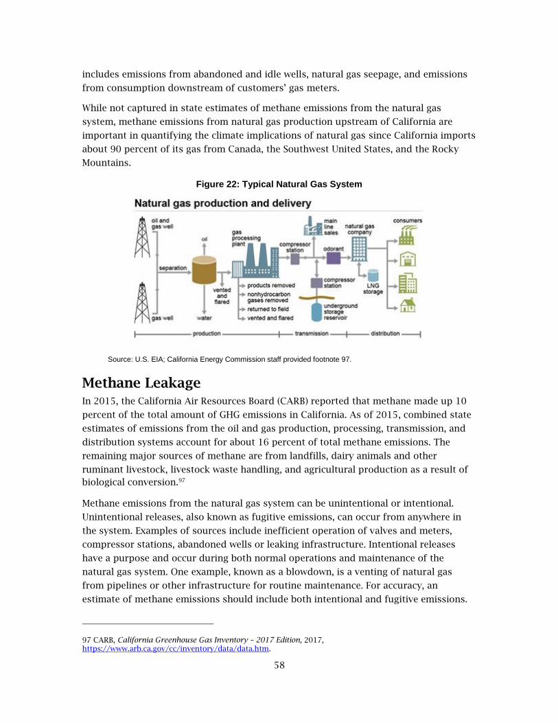
58

includes emissions from abandoned and idle wells, natural gas seepage, and emissions

from consumption downstream of customers’ gas meters.

While not captured in state estimates of methane emissions from the natural gas

system, methane emissions from natural gas production upstream of California are

important in quantifying the climate implications of natural gas since California imports

about 90 percent of its gas from Canada, the Southwest United States, and the Rocky

Mountains.

Figure 22: Typical Natural Gas System

Source: U.S. EIA; California Energy Commission staff provided footnote 97.

Methane Leakage In 2015, the California Air Resources Board (CARB) reported that methane made up 10

percent of the total amount of GHG emissions in California. As of 2015, combined state

estimates of emissions from the oil and gas production, processing, transmission, and

distribution systems account for about 16 percent of total methane emissions. The

remaining major sources of methane are from landfills, dairy animals and other

ruminant livestock, livestock waste handling, and agricultural production as a result of

biological conversion.97

Methane emissions from the natural gas system can be unintentional or intentional.

Unintentional releases, also known as fugitive emissions, can occur from anywhere in

the system. Examples of sources include inefficient operation of valves and meters,

compressor stations, abandoned wells or leaking infrastructure. Intentional releases

have a purpose and occur during both normal operations and maintenance of the

natural gas system. One example, known as a blowdown, is a venting of natural gas

from pipelines or other infrastructure for routine maintenance. For accuracy, an

estimate of methane emissions should include both intentional and fugitive emissions.

97 CARB, California Greenhouse Gas Inventory – 2017 Edition, 2017, https://www.arb.ca.gov/cc/inventory/data/data.htm.

59

Estimating Methane Emissions Bottom-up and top-down are two methods for estimating methane emissions. Both have

advantages and disadvantages, which can cause uncertainties and variability in the

results. The bottom-up method applies emission factors, which are averages based on

measured emissions from specific devices or whole facilities. These emission factors are

multiplied with activity factors for different parts of the system (that is, the number of

compressors or miles of pipeline). The results are totaled from all the components of

the system. The CARB and EPA use this method in their emissions estimations.

The disadvantages of the bottom-up method are associated with the emission factors,

which may not represent the whole population being measured. In some cases, the

technology and age of individual components and whole facilities can be different, so

that taking measurements at only a relatively small amount of facilities will not

represent the whole natural gas system.98

Top-down studies take atmospheric measurements at the facility or regional level.

Aircraft fitted with specialized detection equipment usually perform measurements in

top-down studies. The plane does a complete circle of the study area at various

altitudes. Measurements are taken both upwind and downwind of the source or region.

While taking into account wind velocity, downwind readings subtracted by the upwind

readings determine actual emissions coming from the source area.

The biggest challenge for top-down studies is parsing sources of methane from natural

gas and other anthropogenic and natural sources, or separating readings from natural

gas operations and biogenic sources, like dairy farms.99 To separate natural gas industry

sources from biological sources, tracers such as methane content ratios or stable

isotopes must be identified. However, there are still sources that can frustrate this way

of parsing the data due to natural geologic seepage of methane and emissions from

abandoned wells.

Whether top-down or bottom-up, these studies estimate methane emissions by relying

on assumptions with relatively small test data pools.100 One study found that the largest

5 percent of leaks from natural gas production accounted for at least 50 percent of total

emissions measured.101 That study, along with others, uses the top 5 percent of leaks as

the working definition of super-emitters.102, 103 The relatively low number of super-

98 Brandt, A. R., “Methane Leaks From North American Natural Gas Systems,” Science Magazine, 2014, 343 (6172), pp. 733-735, http://www.novim.org/wp-content/uploads/2011/02/ScienceMethane.02.14.14-1.pdf.

99 Ibid, pp. 733-735.

100 LaCont, R., Methane Emissions in the Natural Gas Life Cycle. April 2015, p. 6. http://westernenergyboard.org/2015/05/final-report-released-by-mj-bradley/.

101 Brandt, A. R., “Methane Leaks from Natural Gas Systems Follow Extreme Distributions,” Environmental Science & Technology, 50 (22), pp. 12,512-12,520, http://pubs.acs.org/doi/abs/10.1021%2Facs.est.6b04303.

102 Ibid, pp. 12,512-12,520.

60

emitters in the system means that the chances of missing one are high when selecting a

sample for study. Findings from a recent review of multiple studies in the United States

indicate that bottom-up and top-down methods can produce similar results.104 Both

have shortcomings, but using a combination of the two techniques can help validate

emissions results.

Researchers have suggested that to realize immediate net climate benefits from using

natural gas instead of dirtier fuel sources, methane emissions from the natural gas

system should be lower than 0.8 percent, 1.4 percent, and 2.7 percent of production to

justify a transition from heavy-duty diesel vehicles, gasoline cars, and coal-fired power

plants, respectively.105 Until there is a more accurate and comprehensive accounting of

methane emissions from the natural gas system, the climate benefits of natural gas as a

transition fuel remain unclear, highlighting the importance of ongoing research in this

area.

Recent Studies In recent years, major research efforts have been undertaken to quantify methane

emissions from all portions of the natural gas system. The Environmental Defense Fund

(EDF), along with industry contribution, is funding and fostering a large-scale

cooperative research effort that examines methane emissions from the natural gas

system. A collection of 16 studies is attempting to improve the understanding and

characterization of methane. Most participants in the project have completed their

studies on the natural gas system, showing estimated leakage rates of about 1.5 percent

of the total gas produced. However, the EDF is still working on an overarching project

synthesis, to develop an overall methane emissions rate across the natural gas supply

chain. This expected to be complete in fall 2017.106

Another paper has synthesized data from EDF’s various published sources and found

that between extraction and delivery, 1.7 percent of the total natural gas produced is

released to the atmosphere (with 95 percent confidence interval from 1.3 and 2.2

103 Zimmerle, Daniel J., “Methane Emissions from the Natural Gas Transmission and Storage System in the United States,” Environmental Science & Technology, 2015, 49 (15), pp. 9374-9383, http://pubs.acs.org/doi/abs/10.1021%2Facs.est.5b01669.

104 Alvarez, M, Joint Agency Methane Symposium, June 6, 2016, p. 92. http://docketpublic.energy.ca.gov/PublicDocuments/16-IEPR-02/TN211181_20160422T102708_Transcript_of_the_04082016_Joint_Agency_Workshop_on_Aliso_Canyo.pdf.

105These numbers were modified from original source of Alvarez et al. 2012 by the Environmental Defense Fund to account for new data. http://docketpublic.energy.ca.gov/PublicDocuments/16-IEPR-02/TN211773_20160609T130055_Methane_Using_New_and_More_Data_to_Manage_Rising_Risk_in_a_Carb.pdf.

106 EDF, Methane Research: The 16 Study Series. http://www.edf.org/sites/default/files/methane_studies_fact_sheet.pdf.

61

percent).107 This compares to the U.S. EPA’s national greenhouse gas inventory implied

methane emission rate of 1.4 percent.

Emissions vary among different parts of the natural gas system. Multiple studies have

examined specific parts of the system. The largest emissions during production are

from pneumatic devices, which are used as liquid levelers, valve controllers, and

pressure regulators. These, as well as other uncharacterized emissions, warrant further

study. A 2015 study found that the gathering of gas from wells and the processing of

the gas to produce pipeline quality gas emits 0.47 percent of total emissions within the

natural gas supply chain.108 Modeling determined that transmission and storage made

up about 0.35 percent of total emissions in 2012. Distribution system emissions were

found to be improving compared to assumptions in previous U.S. EPA greenhouse gas

inventories. This is because distribution system pipelines are being improved with

replacement of older pipeline material (for example, cast iron) with new steel or plastic

pipe.109

State and Federal Greenhouse Gas Inventories The EPA’s latest greenhouse gas inventory report is for 1990 to 2015. The years 2011

through 2015 show a general 5 percent increase in methane emissions from the natural

gas system.

Figure 23 shows the trend of a slight year-over-year increase from 2011 to 2014 and

leveling off in 2015.

107 Littlefield, J. A., “Synthesis of Recent Ground-Level Methane Emission Measurements From the U.S. Natural Gas Supply Chain,” Journal of Cleaner Production, 2017, 148 (17), pp. 9,374-9,383. http://pubs.acs.org/doi/abs/10.1021%2Facs.est.5b01669.

108 Marchese, A. J., “Methane Emissions From United States Natural Gas Gathering and Processing,” Environmental Science and Technology, 2015, pp. 10,718-10,727, http://pubs.acs.org/doi/abs/10.1021/acs.est.5b02275.

109 Lamb, B. K., “Direct Measurements Show Decreasing Methane Emissions From Natural Gas Local Distribution Systems in the United States,” Environmental Science and Technology, 2015, pp. 5161-5169, http://pubs.acs.org/doi/abs/10.1021%2Fes505116p.

62

Figure 23: Methane Emissions From the U.S. Natural Gas System

Source: U.S. EPA, Inventory of U.S. Greenhouse Gas Emissions and Sinks: 1990-2015,

https://www.epa.gov/ghgemissions/inventory-us-greenhouse-gas-emissions-and-sinks-1990-2015.

CARB’s emissions inventory for California separates oil and gas production and

processing from transmission and distribution. In 2015, oil and gas production and

processing made up 6 percent of methane emissions, while transmission and

distribution emissions made up 10 percent of methane emissions; this excludes Aliso

Canyon emissions.110, 111 Figure 24 shows the totals from both sectors between 2010 and

2014.

110 CARB, in making emission estimates from oil and gas extraction, does not separate the emissions attributed to oil production from those produced by natural gas extraction, so methane emissions from natural gas could be understated or overstated.

111 CARB, Short-lived Climate Pollutant Reduction Strategy, Appendix C: California SLCP Emissions, 2017, https://www.arb.ca.gov/cc/shortlived/meetings/11282016/appendixc.pdf.

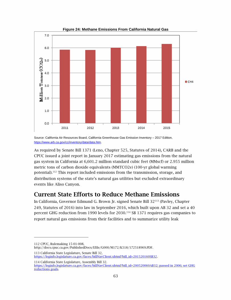
https://www.epa.gov/ghgemissions/inventory-us-greenhouse-gas-emissions-and-sinks-1990-2015

63

Figure 24: Methane Emissions From California Natural Gas

Source: California Air Resources Board, California Greenhouse Gas Emission Inventory – 2017 Edition,

https://www.arb.ca.gov/cc/inventory/data/data.htm.

As required by Senate Bill 1371 (Leno, Chapter 525, Statutes of 2014), CARB and the

CPUC issued a joint report in January 2017 estimating gas emissions from the natural

gas system in California at 6,601.2 million standard cubic feet (MMscf) or 2.955 million

metric tons of carbon dioxide equivalents (MMTCO2e) (100-yr global warming

potential).112 This report included emissions from the transmission, storage, and

distribution systems of the state’s natural gas utilities but excluded extraordinary

events like Aliso Canyon.

Current State Efforts to Reduce Methane Emissions In California, Governor Edmund G. Brown Jr. signed Senate Bill 32113 (Pavley, Chapter

249, Statutes of 2016) into law in September 2016, which built upon AB 32 and set a 40

percent GHG reduction from 1990 levels for 2030.114 SB 1371 requires gas companies to

report natural gas emissions from their facilities and to summarize utility leak

112 CPUC, Rulemaking 15-01-008, http://docs.cpuc.ca.gov/PublishedDocs/Efile/G000/M172/K518/172518969.PDF.

113 California State Legislature, Senate Bill 32, https://leginfo.legislature.ca.gov/faces/billNavClient.xhtml?bill_id=201520160SB32.

114 California State Legislature, Assembly Bill 32. https://leginfo.legislature.ca.gov/faces/billNavClient.xhtml?bill_id=200520060AB32; passed in 2006; set GHG reductions goals.

https://www.arb.ca.gov/cc/inventory/data/data.htm

64

management practices, among other things.115 CARB and the CPUC prepare joint annual

reports to track and analyze natural gas emissions from the transmission, distribution,

and storage activities throughout the state.

CARB and CPUC staff indicated that gas system operators should use the information

from these reports to help determine where they can achieve emission reductions to

meet the state’s methane emission reduction goal, while maintaining the safe and

reliable operation of the regulated gas storage and delivery systems.116

At its June 15, 2017, meeting, the CPUC took the following actions as part of its SB 1371

proceeding:

Instituted annual reporting for tracking methane emissions.

Approved 26 mandatory best practices for minimizing methane emissions.

Required a biennial compliance plan incorporated into the utilities’ annual gas

safety plans, beginning in March 2018.

Instituted a cost recovery process to simplify CPUC review and approval of

incremental expenditures to implement best practices,117 which included

expenditures for pilot programs and research and development.

SB 1383 requires CARB, CPUC, and the Energy Commission to “undertake various

actions related to reducing short-lived climate pollutants in the state.” The bill focuses

attention on reducing methane emissions from dairy and organic wastes by containing

methane and using it as a renewable gas.118 The legislation also directs CARB to begin

implementing a short-lived climate pollutant strategy with the goal of reducing methane

emissions by 40 percent below 2013 levels by 2030.119, 120

As part of the work to reduce short-lived climate pollution, the Energy Commission

funds methane emission research through its natural gas research and development

program. This research found evidence that fugitive emissions occur in every subsector

115 California State Legislature, Senate Bill 1371. https://leginfo.legislature.ca.gov/faces/billNavClient.xhtml?bill_id=201320140SB1371.

116 CARB and CPUC, Joint Staff Report: Analysis of the Utilities' June 17, 2016, Methane Leak and Emissions Reports, required by SB 1371, p. 3.

117 At this time, only the proposed decision is available on the CPUC’s website: http://docs.cpuc.ca.gov/PublishedDocs/Efile/G000/M186/K437/186437714.PDF.

118 The Draft 2017 Integrated Energy Policy Report to be released later this fall is expected to include a discussion of cost-effective strategies and priority end uses of renewable gas in relation to existing state policies and climate goals. Emerging opportunities for renewable gas resource and technology solutions to reach longer-term SLCP goals will also be addressed.


120 California State Legislature, Assembly Bill 1257, https://leginfo.legislature.ca.gov/faces/billNavClient.xhtml?bill_id=201320140AB1257.

65

throughout the natural gas system, including homes, natural gas vehicle refilling

stations, and plugged and abandoned natural gas wells.

Other projects related to methane emissions include research to:

Characterize fugitive emissions from commercial buildings in California

Study the potential impacts of subsidence (vertical and horizontal changes in

elevation due to groundwater extraction during the drought) to the natural gas

system and methane emissions from abandoned wells

Senate Bill 605 (Lara, Chapter 523, Statutes of 2014) requires CARB to develop strategies

that further reduce short-lived climate pollutants, such as methane.121 In general, the

latest proposed regulations associated with the natural gas system, suggest greater,

mandatory monitoring on a wider assortment of components than was previously

considered. New laws and regulations are also pushing for better mitigation strategies

for emissions from pipelines.122

The data and associated studies from SB 605 will be used in the CARB/CPUC annual

joint staff report that analyzes the utilities’ emission reports. This work will improve

understanding of the amount of emissions from utilities’ facilities and pipelines.

State agency efforts to reduce methane emissions from natural gas system

infrastructure are ongoing. CARB staff are working with local air quality districts to

develop new regulations, which will include vapor collection from high-emitting storage

tanks and other equipment, leak detection and repair on more components then covered

by local air districts, and ambient methane monitoring and more frequent wellhead

monitoring at underground gas storage facilities.

CARB is also cooperating with DOGGR on above- and below-ground monitoring of

storage facilities. CARB proposed improved above-ground methane monitoring of

underground storage facilities in the agency’s Oil and Gas Production, Processing and

Storage Regulation program to implement some requirements of SB 887. DOGGR is

formalizing and adding to the emergency regulations implemented in February 2016.

The new regulations are expected to be completed in 2017.

Assembly Bill 1496 (Thurmond, Chapter 604, Statutes of 2015) calls on CARB to monitor

and measure high-methane emission hot spots and to conduct a life-cycle GHG emission

study for natural gas produced in and imported into California.

In early 2017, the Energy Commission approved more than $5 million in grants for

research examining the natural gas system. The approved projects include:


122 CARB, Short-Lived Climate Pollutant Reduction Strategy, March 2017, pp. 79-80. https://www.arb.ca.gov/cc/shortlived/meetings/03142017/final_slcp_report.pdf.

66

$1.1 million to Energy and Environmental Economics, Inc. to assess long-term

technology pathways for natural gas systems to meet energy and GHG emission

goals

$1.6 million to Lawrence Berkeley National Laboratory to research new

technology to identify areas with high risk of natural gas infrastructure damage

due to land subsidence and to recommend remedial actions

$597,433 grant to University of California, Davis, to survey methane leakage

from abandoned and plugged natural gas wells in California

$1.4 million to the Electric Power Research Institute to address fugitive GHG

emissions, including methane and nitrous oxide, at industrial plants.

67

Tracking Natural Gas Emissions In the past few years, California has developed new regulations and policies to improve

the monitoring, reporting, and repairing of its natural gas infrastructure and exceed

federal requirements. These new regulations and reporting requirements will provide

information and data on the state’s natural gas infrastructure. About 90 percent of the

gas used in California is imported from outside the state, and the emissions associated

with these imports are not well understood. Senate Bill 839 (Committee on Budget and

Fiscal Review, Chapter 340, Statutes of 2016) requires the Energy Commission to report

on the resources needed to develop a system that would allow California to track

emissions from both in-state and out-of-state emissions. The tracking system is

intended to provide CARB with the data it needs to model emissions. The Energy

Commission is working with CARB to determine the most appropriate data to collect.

Staff recently completed a progress report, which will be available in fall 2017.

68

ACRONYMS

Acronym Proper Name

AAEE additional achievable energy efficiency

AB Assembly Bill

BAA balancing area authorities

Bcf billion cubic feet

BLM Bureau of Land Management

California ISO California Independent System Operator

CED California Energy Demand

CHP combined heat and power

CPUC California Public Utilities Commission

EE energy efficiency

Energy Commission California Energy Commission

Fracking hydraulic fracturing

GDP gross domestic product

GHG greenhouse gas

GTN Gas Transmission Northwest Company

GW gigawatt

GWh gigawatt-hours

IEPR Integrated Energy Policy Report

IOU investor-owned utility

LADWP Los Angeles Department of Water and Power

LNG liquefied natural gas

MAPE mean absolute percentage error

MMBtu million British thermal unit

MW megawatt

NAMGas North American Market Gas-Trade Model

69

NGCC Natural gas combined-cycle

NYMEX New York Mercantile Exchange

OTC once-through cooling

PEMEX Petróleos Mexicanos

PG&E Pacific Gas and Electric Company

POU publicly owned utilities

PSEP Pipeline Safety Enhancement Plan

PV photovoltaic

QFER Quarterly Fuels and Energy Report

RPS Renewables Portfolio Standard

SB Senate Bill

SCE Southern California Edison Company

SDG&E San Diego Gas & Electric Company

SMUD Sacramento Municipal Utility District

SoCalGas Southern California Gas Company

SWRCB State Water Resources Control Board

Tcf trillion cubic feet

TEPPC Transmission Electric Planning and Policy Committee

U.S. United States

U.S. EPA United States Environmental Protection Agency

U.S. EIA United States Energy Information Administration

WECC Western Electricity Coordinating Council

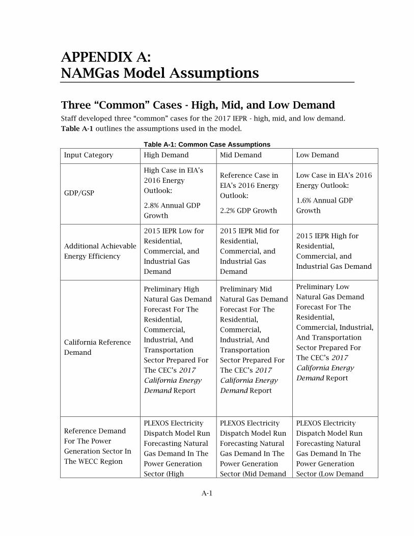
A-1

APPENDIX A: NAMGas Model Assumptions

Three “Common” Cases - High, Mid, and Low Demand Staff developed three “common” cases for the 2017 IEPR - high, mid, and low demand.

Table A-1 outlines the assumptions used in the model.

Table A-1: Common Case Assumptions

Input Category High Demand Mid Demand Low Demand

GDP/GSP

High Case in EIA's

2016 Energy

Outlook:

2.8% Annual GDP

Growth

Reference Case in

EIA's 2016 Energy

Outlook:

2.2% GDP Growth

Low Case in EIA's 2016

Energy Outlook:

1.6% Annual GDP

Growth

Additional Achievable

Energy Efficiency

2015 IEPR Low for

Residential,

Commercial, and

Industrial Gas

Demand

2015 IEPR Mid for

Residential,

Commercial, and

Industrial Gas

Demand

2015 IEPR High for

Residential,

Commercial, and

Industrial Gas Demand

California Reference

Demand

Preliminary High

Natural Gas Demand

Forecast For The

Residential,

Commercial,

Industrial, And

Transportation

Sector Prepared For

The CEC’s 2017

California Energy

Demand Report

Preliminary Mid

Natural Gas Demand

Forecast For The

Residential,

Commercial,

Industrial, And

Transportation

Sector Prepared For

The CEC’s 2017

California Energy

Demand Report

Preliminary Low

Natural Gas Demand

Forecast For The

Residential,

Commercial, Industrial,

And Transportation

Sector Prepared For

The CEC’s 2017

California Energy

Demand Report

Reference Demand

For The Power

Generation Sector In

The WECC Region

PLEXOS Electricity

Dispatch Model Run

Forecasting Natural

Gas Demand In The

Power Generation

Sector (High

PLEXOS Electricity

Dispatch Model Run

Forecasting Natural

Gas Demand In The

Power Generation

Sector (Mid Demand

PLEXOS Electricity

Dispatch Model Run

Forecasting Natural

Gas Demand In The

Power Generation

Sector (Low Demand

A-2

Input Category High Demand Mid Demand Low Demand

Demand Case) For

The WECC Region

Case) For The WECC

Region

Case) For The WECC

Region

Reference Demand

for the Residential,

Commercial,

Industrial, and

Transportation Sector

Outside of California.

Reference Demand

for the Power

Generation Sector

Outside of The WECC

Region

Small “m”

Econometric Model

(High Demand Case)

Small “m”

Econometric Model

(Mid Demand Case)

Small “m” Econometric

Model

(Low Demand Case)

Renewables 50% by 2030 50% by 2030 50% by 2030

Coal Retirement

Through 2050 73 GW 53 GW 33 GW

Resource Capital

Costs

30% Lower Than

2015 Inputs 2015 Inputs

30% Higher Than 2015

Inputs

Resource O&M Costs 30% Lower Than

2015 Inputs 2015 Inputs

30% Higher Than 2015

Inputs

Proved Supply Forward Costs

30% Lower Than Reference Case (2017 And After)

Estimate Based on Hub Prices

30% Higher Than Reference Case (2017 And After)

Source: California Energy Commission staff.

B-1

APPENDIX B: Burner Tip Method

Actual burner tip prices include a commodity price and a transportation rate, both of

which are assessed per unit of natural gas. The commodity price is the price of natural

gas after production from the well and processing for injection into a nearby utility

pipeline. The transportation rate is the cost of transporting the gas from its injection

point near the production basin to the electric generator for consumption. Actual

commodity prices and transportation rates are publicly available, with the former as an

average of actual transactions. Commodity prices are provided by industry journals,

such as Natural Gas Intelligence, which publish average wholesale volume-weighted

prices from surveys of monthly “bidweek” transactions at more than a hundred pricing

points across North America.123

Transportation rates are published in the tariffs posted by the natural gas pipeline

operators on their websites and are also filed with regulators. Energy Commission staff

learned from discussions with industry personnel that generators procure most natural

gas on contract and are indexed to a bidweek price at one of these pricing points. Actual

power plant burner tip prices usually include additional contract costs such as

procurement, price risk, transactions, and others. The terms of these contracts are

proprietary and not publicly available. Consequently, no model, including the Burner Tip

Model, can account for these costs. The model is the best estimate developed by staff,

using publicly available information.

123 Market participants in the natural gas industry buy much of their physical natural gas, or gas they will consume, for the upcoming month as part of a process called bidweek.

C-1

APPENDIX C: PLEXOS Modeling Assumptions

There are several assumptions made to align with other planning exercises. The

following sections discuss assumptions in which analyses show that the results are

sensitive to changes. Energy Commission staff’s WECC-wide production simulation

model dataset covers 2017 through 2030 for the three common cases for the 2017 IEPR

and one other case with a higher level of AAEE.124

Table C-1 summarizes these cases.

Table C-1: IEPR Common Cases

Common Case 2017 IEPR Preliminary

Load Forecast Energy Efficiency* RPS Target

High Energy Consumption High Low 2016 IEPR Update AAEE

50% by 2030

Mid Energy Consumption Mid Mid AAEE 50% by 2030

Low Energy Consumption Low High AAEE 50% by 2030

Source: California Energy Commission staff.

*Uses 2016 IEPR Update because 2017 AAEE data are not yet available.

Diablo Canyon Retirement The Diablo Canyon power plant is retired in all IEPR common cases. The model assumes

Diablo Canyon Unit 1 is retired December 31, 2024, and Unit 2 by August 26, 2025.

Consistent with the Diablo Canyon Retirement Proposal, all common cases include 2,000

GWh of gross energy efficiency in addition to the AAEE already embedded in the IEPR

common cases and an additional 2,000 GWh/yr of new renewables developed between

2020 and 2024.

Hourly Net Export Constraint Staff imposed an hourly net export constraint of 4,000 MW in all IEPR common cases.

The CPUC’s Draft 2017 Assumptions and Scenarios for Long-Term Planning125

recommend 2,000 MW for all cases except the interregional coordination scenario, which

assumes 5,000 MW. Staff used 4,000 MW because the IEPR simulations are statewide,

while the CPUC assumptions are for California ISO’s area only. This constraint allows

the production cost model to curtail zero-cost renewable power since renewable energy

124 Additional achievable energy efficiency is savings from initiatives that are planned but not yet approved by the utilities or any other entity.

125 CPUC, http://docs.cpuc.ca.gov/PublishedDocs/Efile/G000/M172/K519/172519400.PDF.

http://docs.cpuc.ca.gov/PublishedDocs/Efile/G000/M172/K519/172519400.PDF

C-2

resources in certain hours that are in excess of loads are considered transmission

constrained. The renewable curtailments are below 100 GWh per year in all cases until

2028. The mid demand case consistently has the lowest amount of renewable

curtailment, while the low and high demand cases consistently incur the highest amount

of renewable curtailments. Figure C-1 shows the amount of annual renewable

curtailments by case.

Figure C-1: Annual Renewable Curtailments by Case

Source: California Energy Commission, PLEXOS results.

Load Forecast for Non-California WECC (2017 to 2030) Staff used data submitted to the WECC by balancing area authorities (BAAs) for 2015

and the WECC TEPPC 2026 common case126 load forecast as “bookends” to estimate the

non-California BAA load. Staff used a compound annual growth rate formula to

calculate the peak and energy demand for the intervening years (2017 to 2025). The

period for 2017 IEPR PLEXOS simulations extended beyond the TEPPC common case

year of 2026, so staff used the compound annual growth rate to extrapolate the forecast

by four years to 2030. Staff used the annual peak and energy forecasts as inputs to

PLEXOS, and developed hourly energy profiles (GWh) and regional peak demand (MW)

for each year using the “build”127 function embedded in the PLEXOS software.

126 WECC, Datasets, https://www.wecc.biz/SystemAdequacyPlanning/Pages/Datasets.aspx#f727be3b-b212-4e51-8f5d-538497ae357d=%7B%22k%22%3A%22%22%7D#c6981a26-5370-44c9-b968-8836159a8cae=%7B%22k%22%3A%22%22%7D#0cf7cc46-0612-4858-a694-967947be8e76=%7B%22k%22%3A%22%22%2C%22s%22%3A21%7D#db6a7e9a-a52d-42ad-88b9-e742744164ad=%7B%22k%22%3A%22%22%7D.

127 The linear programming model uses the peak and energy forecast and an average hourly load profile for load-serving entities in the WECC to develop hourly profiles for 2017 – 2030.

C-3

Staff developed energy (GWh) and peak (MW) forecasts for the high demand/low price

and low demand/high price cases using different multipliers for each BAA by using data

from the U.S. EIA. The U.S. EIA provided data for high and low electricity demand cases

by region (Northwest, Southwest, and Rocky Mountains).128 To calculate the high and low

demand cases, staff again used compound growth formulas for each region for each

year of the forecast period. Figure C-2 displays the annual WECC (Non-California) load

forecast in GWh for the period of 2017 to 2030 for all three common cases. Staff

calculated annual peak demand for each BAA using the same method. Because different

regions experience system peak at different times of the year (summer or winter) and

different times of the day, aggregated, or combined, peak demand data are not

presented here.

Figure C-2: WECC (Non-CA) Electricity Load Forecast—All Cases (GWh)

Source: California Energy Commission.

Hydro Generation Forecast Continuing the 2015 IEPR hydro generation input assumption technique, staff

developed WECC-wide hydroelectric generation input data using a shorter and more

recent set of historical hydro generation data from the U.S. EIA.129 This method is used

to reflect the overall trend of reduced hydroelectric generation due to persistent or

semipersistent drought conditions in the western United States and to reflect changes in

hydroelectric operations due to federal and state regulations concerning water flows for

fish protection.

128 U.S. EIA, Annual Energy Outlook, https://www.eia.gov/outlooks/aeo/data/browser/#/?id=8-AEO2016&region=0-0&cases=ref2016~highmacro~lowmacro&start=2017&end=2030&f=A&linechart=~~~ref2016-d032416a.56-8-AEO2016~highmacro-d032516a.56-8-AEO2016~lowmacro-d032516a.56-8-AEO2016&ctype=linechart&sourcekey=0

129 See U.S. EIA’s website at: http://www.eia.gov/electricity/monthly/.

C-4

Historically, staff has used the hydroelectric generation data from 1991 to the most

recent year for which a complete set of plant data is available (2015). For this IEPR cycle,

staff used hydroelectric generation data from 2001 to 2015 to calculate the average

monthly generation by hydroelectric plant. Data for calendar year 2016 were not

complete at the time of simulation runs, and staff does not anticipate them being ready

for publication by U.S. EIA until October 2017. Due to a lack of available data, staff did

not update the Canadian hydroelectric generation forecast for Alberta and British

Columbia, but recent information posted on the BC Hydro, Columbia Power, and Fortis

B.C. websites are consistent with PLEXOS inputs for British Columbia’s hydro generation.

The monthly projections for California hydroelectric generation are an average based on

plant level 2001 to 2015 monthly historical generations. However, since 2016, California

has seen an increase in precipitation activity and associated hydroelectric output. As

such, staff inflated the 2017 average monthly hydro generation input for California

plants using recent data submittals to reflect the projected increase in hydro generation.

This adjustment will better reflect hydro performance and result in a reduction in the

amount of California gas-fired generation in PLEXOS simulations for 2017. Staff did not

make similar adjustments to hydro conditions for the rest of the Western Interconnect.

Unit Commits For this modeling cycle, staff analyzed roughly 80 out-of-state coal and combined-cycle

generators throughout the Western Interconnect. Staff sought to update a modeling

characteristic of these plants to forecast and provide more accurate data.

Each generator has unique properties. It is important to assign qualities and date to a

simulated generator that reflects the real world. One such characteristic is a unit

commit. Setting a unit commit tells the modeling software how the generator should

operate. There are three basic settings the generator can have: always on (constantly

running), off (not running), or optimized (running according to when it is most

economically efficient and profitable). Setting the commit status to "always on" is often

best for baseload generators such as coal facilities. Occasionally, staff needs to update

the plants in the simulation so that the model can predict more accurate outcomes. This

is due to factors such as changes in market fuel prices or announced plant retirements.

Staff analyzed and compared the historical trend to the results of the sample plants in

two scenarios. The first scenario tested the plant units running always on with a few

running in the optimized setting. The second scenario tested the opposite with the

majority of the plant units running an optimized case with a minority in a must-run

case. Staff gathered five-year historical data from sources including U.S. EIA and the U.S.

EPA’s Continuous Emission Monitoring reporting. Staff sought to compare the best fit

for each generator based on either simulated scenario to the actual historical data.

After reviewing the results, staff agreed on an appropriate commit status for the

analyzed generators to reflect more accurate results. Staff decided that almost a third of

the generators would be set as must-runs while the remaining would be run

C-5

economically. A few plant units in Nucla, Colorado, and Mesquite, Arizona, fit neither

scenario. Staff decided to split the commit status by months. In general, they would be

operating as must-runs for the summer months while running economically the rest of

the year.

Renewable Energy Build–Out Targets In all three cases, demand for conventional generation decreases over the forecast

period, as states are assumed to achieve more aggressive renewable energy targets.

Table C-2 lays out the energy build-out targets assumed in this modeling cycle.

Table C-2: Energy Build-Out Targets by State

2017 2020 2024 2027 2030

Arizona 4.20 6.10 8.70 9.40 9.60

Colorado 5.80 10.70 11.00 11.40 11.60

Montana 1.50 1.60 1.60 1.60 1.60

New Mexico 2.70 3.80 3.90 3.90 4.00

Nevada 4.70 6.10 6.20 8.10 8.30

Oregon 4.90 6.90 7.00 9.90 12.80

Utah 3.13 4.43 6.16 7.46 8.76

Washington 6.60 11.30 11.40 11.40 11.50

Alberta 4.76 7.52 11.20 13.96 15.80

Sources: Barbose, Galen L., U.S. Renewables Portfolio Standards: 2017 Annual Status Report, 2017, WECC Transmission

Expansion Planning Policy Committee 2026 Common Case, and AESO 2017 Long-term Outlook,

https://www.aeso.ca/grid/forecasting/

https://www.aeso.ca/grid/forecasting/

D-1

APPENDIX D: Detailed Method for Historical and Forecasted Rates

The following sections describe the method for the historical and forecasted data set for

the three utilities: PG&E, SoCalGas and SDG&E.

Pacific Gas and Electric End-Use Rates

Residential

For the 1967 to 1990 historical rates, staff used PG&E’s annual statistical reports.130

Staff divided the reported total revenues by total volumes to devise the rates. For 1990

to 1996 historical rates, staff used the Energy Commission’s Quarterly Fuels and Energy

Report (QFER) form 7 and 1308 schedule 3. For the 1997 to 2015 rates, staff used the

U.S. EIA’s Natural Gas Annual Respondent Query System (EIA-176) to populate the

data.131

For forecasted rates, staff added transportation and public purpose program surcharges

(PPPS) to NAMGas modeled PG&E hub rates. PG&E posts the current transportation and

PPPS on the California Gas Transmission, Pipe Ranger website.132 Staff used weighted

averages for both the transportation and PPPS. Staff escalated the transportation charge

from 2017 to 2026 by the Bureau of Labor Statistics’ (BLS) utility-piped gas consumer

price index (CPI) 12-month average – 0.82 percent as of December 2016.133

Commercial and Industrial

For the 1967 to 1990 rates, staff interpolated the data. Staff used average percentage

differences between residential and commercial/industrial for the known data years

(1990 to 2015), and then multiplying the residential rate by the average percentage to

interpolate historical rates for commercial and industrial. For 1990 to 1996, staff used

the Energy Commission’s QFER form 7 and 1308, schedule 3. For the 1997 to 2015 rates,

130 PG&E, Financials, http://investor.pgecorp.com/financials/annual-reports-and-proxy-statements/.

131 U.S. EIA, http://www.eia.gov/cfapps/ngqs/ngqs.cfm?f_report=RPC&f_sortby=&f_items=&f_year_start=&f_year_end=&f_show_compid=&f_fullscreen=.

132 PG&E, http://www.pge.com/tariffs/tm2/pdf/GAS_SCHEDS_G-PPPS.pdf, http://www.pge.com/tariffs/tm2/pdf/GAS_SCHEDS_G-1.pdf.

133 BLS, News Release, August 2017, https://www.bls.gov/news.release/pdf/cpi.pdf.

https://www.bls.gov/news.release/pdf/cpi.pdf

D-2

staff used U.S. EIA’s Natural Gas Annual Respondent Query System (EIA-176)134 to

populate the data.

For forecasted rates, staff added transportation and public purpose program surcharges

(PPPS) to NAMGas-modeled PG&E hub rates. PG&E posts the current transportation and

PPPS on the California Gas Transmission, Pipe Ranger website.135 Staff used weighted

averages for both the transportation and PPPS. Staff escalated the transportation charge

from 2017 to 2026 by the BLS CPI 12-month average – 0.82 percent as of December

2016.136

Southern California Edison/Southern California Gas Company Since SCE does not service natural gas, staff used SoCalGas as a proxy for the SCE

electricity planning area.

Residential

For the 1967 to 1996 historical rates, staff used SoCalGas’ annual statistical reports.137

Staff divided the reported total revenues by total volumes. For 1990 to 1996 historical

rates, staff used the Energy Commission’s QFER form 7 and 1308 schedule 3. For the

1997 to 2015 rates, staff used EIA’s Natural Gas Annual Respondent Query System (EIA-

176)138 to populate the data.

For forecasted rates, staff added transportation charges and PPPS to NAMGas-modeled

SoCalGas hub rates. SoCalGas posts the charges on the SoCalGas ENVOY website.139 Staff

used weighted averages for both the transportation charges and PPPS. Staff escalated

the transportation charge from 2017 to 2026 by the BLS’ utility-piped gas CPI 12-month

average, 0.82 percent as of December 2016.140

Commercial and Industrial

For the 1967 to 1990 historical rates, staff interpolated the data. Staff used average

percentage differences between residential and commercial/industrial for the known

data years (1990 to 2015), then multiplying the residential rate by the average


135 PG&E, http://www.pge.com/tariffs/tm2/pdf/GAS_SCHEDS_G-1.pdf .


137 Sempra Energy, Financial Reports, http://investor.shareholder.com/sre/annuals.cfm.


139 SoCalGas, https://scgenvoy.sempra.com/.

140 BLS, News Release, https://www.bls.gov/news.release/pdf/cpi.pdf.

http://www.eia.gov/cfapps/ngqs/ngqs.cfm?f_report=RPC&f_sortby=&f_items=&f_year_start=&f_year_end=&f_show_compid=&f_fullscreen


http://www.pge.com/tariffs/tm2/pdf/GAS_SCHEDS_G-1.pdf



http://investor.shareholder.com/sre/annuals.cfm



https://scgenvoy.sempra.com/

https://www.bls.gov/news.release/pdf/cpi.pdf

D-3

percentage to interpolate historical rates for commercial and industrial. For 1990 to

1996, staff used the Energy Commission’s QFER form 7 and 1308 schedule 3. For the

1997 to 2015 rates, staff used EIA’s Natural Gas Annual Respondent Query System (EIA-

176)141 to populate the data.

For forecasted rates, staff used the same methodology as residential with adjustments

to the transportation and public purpose program charges.

San Diego Gas & Electric End-Use Rates

Residential

For the 1997 to 2015 rates, staff used U.S. EIA’s Natural Gas Annual Respondent Query

System (EIA-176).142 For the 1967 to 1996 rates, staff used Sempra’s Annual Statistical

Report,143 taking total revenues divided by total volume.

For forecasted rates, staff added weighted average transportation and PPPS charges to

NAMGas-modeled SDG&E hub rates. The transportation and PPPS charges come from

SDG&E’s tariff rates posted online at the SoCalGas ENVOY website.144 Staff escalated the

transportation charge from 2017 to 2026 by the BLS’ utility-piped gas CPI 12-month

average – 0.82 percent as of December 2016.145

Commercial

For the 1997 to 2015 rates, staff used the same method as residential rates. For 1990 to

1996, staff used the Energy Commission’s QFER form 7 and 1308 schedule 3. For the

1967 to 1990 rates, staff interpolated data. Staff used average percentage differences

between residential and commercial for the known data years (1990 to 2015), then

multiplied the residential rate by the average percentage to interpolate historical rates

for commercial.

Industrial

For the 1967 to 1990 rates, staff interpolated data. Staff used average percentage

differences between residential and commercial for the known data years (1997 to

2015), then multiplied the residential rate by the average percentage to interpolated

historical rates for commercial and industrial. For the 1997 to 2015 rates staff obtain

total commercial and industrial volumes and revenues from SDG&E’s annual Statistical

Reports, then obtain commercial volumes and revenues from U.S. EIA’s Natural Gas

Annual Respondent Query System, EIA-176. Staff found the difference between


142 U.S. EIA, cbid.

143 SDG&E, http://investor.shareholder.com/sre/annuals.cfm.

144 SoCalGas, https://scgenvoy.sempra.com.

145 BLS, News Release, https://www.bls.gov/news.release/pdf/cpi.pdf.



http://investor.shareholder.com/sre/annuals.cfm

https://scgenvoy.sempra.com/

D-4

commercial volumes and revenues from totals in the annual statistical report and U.S.

EIA’s data to find industrial volumes and revenues, then divided revenues by volumes to

get an implied rate. Table D-1 through

D-5

Table D-3 display PG&E, SoCalGas, and SDG&E modeling results.

Table D-1: Modeling Results for PG&E, Reference Case

2016$/Mcf Residential Commercial Industrial

2017 $14.79 $11.53 $6.65

2018 $14.94 $11.65 $6.72

2019 $15.31 $11.99 $7.00

2020 $15.52 $12.18 $7.14

2021 $15.65 $12.26 $7.18

2022 $15.78 $12.36 $7.23

2023 $15.92 $12.47 $7.29

2024 $16.07 $12.57 $7.34

2025 $16.23 $12.71 $7.42

2026 $16.39 $12.84 $7.50

2027 $16.56 $12.96 $7.57

2028 $16.67 $13.05 $7.59

2029 $16.84 $13.18 $7.67

2030 $17.01 $13.31 $7.75


D-6

Table D-2: Modeling Results for SoCalGas, Reference Case

2016$/Mc

f Residential Commercial Industrial

2017 $9.58 $7.57 $7.57

2018 $9.68 $7.65 $7.65

2019 $9.99 $7.95 $7.95

2020 $10.15 $8.09 $8.09

2021 $10.22 $8.14 $8.14

2022 $10.30 $8.21 $8.21

2023 $10.40 $8.28 $8.28

2024 $10.48 $8.34 $8.34

2025 $10.59 $8.44 $8.44

2026 $10.70 $8.52 $8.52

2027 $10.80 $8.61 $8.61

2028 $10.87 $8.65 $8.65

2029 $10.98 $8.74 $8.74


D-7

Table D-3: Modeling Results for SDG&E, Reference Case

2016$/Mcf Residential Commercial Industrial

2017 $13.87 $7.56 $7.56

2018 $14.02 $7.66 $7.66

2019 $14.38 $7.95 $7.95

2020 $14.60 $8.10 $8.10

2021 $14.71 $8.14 $8.14

2022 $14.84 $8.21 $8.21

2023 $14.98 $8.28 $8.28

2024 $15.12 $8.35 $8.35

2025 $15.28 $8.45 $8.45

2026 $15.43 $8.53 $8.53

2027 $15.59 $8.61 $8.61

2028 $15.69 $8.65 $8.65

2029 $15.86 $8.74 $8.74

2030 $16.03 $8.84 $8.84

Source: California Energy Commission, Supply Analysis Office.

E-1

APPENDIX E: Comparison of Gas Price Forecasts

This appendix compares the Energy Commission’s NAMGas model results of natural gas

prices at Henry Hub to other forecasts of Henry Hub prices. The comparison includes

the following forecasts, along with the date of release:

U.S. EIA Annual Energy Outlook (January 2017)

Northwest Power and Conservation Council (NWPCC), The Seventh Power Plan

Proposed Fuel Price Forecasts (February 2016)

U.S. EIA, Annual Energy Outlook, January 2017 The U.S. EIA ran several natural gas price cases.146 Staff examined cases that are most

comparable to the Energy Commission’s staff assessment of natural gas price forecast.

Three cases were used: 1) U.S. EIA’s reference case, 2) low oil and gas resources and

technology, and 3) high oil and gas resources and technology.

In the reference case, U.S. EIA assumes population growth of 0.7 percent per year and

GDP increases of 2.2 percent per year, with 2.6 percent GDP growth in the high resource

case and 1.6 percent growth in the low resource case, the same as the Energy

Commission’s assumptions.

In the low oil and gas resource and technology case, the estimated ultimate recovery per

tight oil, tight gas, or shale gas in the United States and undiscovered resources in

Alaska and the offshore Lower 48 states is assumed to be 50 percent lower than in the

reference case. Rates of technology improvement that reduce costs and increase

productivity in the United States are also 50 percent lower than in the reference case.

These assumptions increase the per-unit cost of crude oil and natural gas development

in the United States. The total unproved technically recoverable resource of crude oil is

decreased to 150 billion barrels, and the natural gas resource is decreased to 1,303

trillion cubic feet (Tcf), as compared with unproved resource estimates of 238 billion

barrels of crude oil and 2,136 Tcf of natural gas as of January 1, 2014, in the reference

case.

In the high oil and gas resource and technology case, the resource assumptions are

adjusted to allow a continued increase in domestic crude oil production through 2040,

to 18 million barrels per day (bpd) compared with 11 million bpd in the reference case.

This case includes:

146 For more on U.S. EIA’s AEO 2017, see https://www.eia.gov/outlooks/aeo/.

https://www.eia.gov/outlooks/aeo/

E-2

Fifty percent higher estimated ultimate recovery per tight oil, tight gas, or shale

gas well, as well as additional unidentified tight oil and shale gas resources to

reflect the possibility that additional layers or new areas of low-permeability

zones will be identified and developed

Diminishing returns on the estimated ultimate recovery once drilling levels in a

county exceed the number of potential wells assumed in the reference case, to

reflect well interference at greater drilling density

Fifty percent higher assumed rates of technological improvement that reduce

costs and increase productivity in the United States relative to the reference

case

Fifty percent higher technically recoverable undiscovered resources in Alaska

and the offshore Lower 48 states than in the reference case. The total unproved

technically recoverable resource of crude oil increases to 385 billion barrels,

and the natural gas resource increases to 3,109 Tcf as compared with unproved

resource estimates of 238 billion barrels of crude oil and 2,136 Tcf of natural

gas in the reference case as of the start of 2014.147

Comparing U.S EIA to Energy Commission Forecast The U.S. EIA uses the National Energy Modeling System, while Energy Commission staff

uses the Market Builder platform. Due to the different algorithms used, it may not be

possible to have the same assumptions in both models. Even with the same

assumptions, it may not be possible to see the same results. Comparisons based on

estimates, however, are feasible.

Both reference cases follow the same basic trajectory through 2030. The U.S. EIA’s

reference case starts at $3.11 Mcf (in 2016$) in 2017 and climbs to $5.19 Mcf in 2030;

whereas the Energy Commission's prices start at $3.11 Mcf in 2017 and rise to $4.54

Mcf in 2030, a 14 percent difference in price in 2030.

The U.S. EIA’s high oil and gas resource and technology case prices are higher than the

Energy Commission’s through 2030. The Energy Commission’s prices are 66 percent

lower ($3.88 vs $2.33 Mcf) in 2030. For the U.S. EIA’s low oil and gas resource and

technology case, prices start higher in 2017 compared to the Energy Commission’s

($3.29 vs $3.15). The U.S. EIA’s forecasted prices climb higher until 2030, when the

Energy Commission’s prices exceed those of the U.S. EIA’s. The U.S. EIA’s 2030 price of

$8.26 Mcf is 5 percent lower than the Energy Commission’s price of $8.66 per Mcf.

Both modeling efforts have similar economic growth, demands, cost variations and

supplies. The price differences in the first few years can be attributed to how the

147 For more on U.S. EIA’s assumptions, see https://www.eia.gov/outlooks/aeo/assumptions/pdf/introduction.pdf.

E-3

differing models work. The U.S. EIA’s model has a more gradual inclusion of the change

in resources and costs, while NAMGas’ inclusion of these takes effect immediately. The

Energy Commission’s forecast trends lower than U.S. EIA’s partially because NAMGas’

total recoverable resources are higher than U.S. EIA’s 188 Tcf in the mid demand or

reference cases. Figure E-1 compares U.S. EIA’s price projections with that of the Energy

Commission and Henry Hub.

Figure E-1: Henry Hub Prices, U.S. EIA vs. Energy Commission

Source: U.S. EIA AEO 2017 and California Energy Commission, Supply Analysis Office.

NWPCC, Fuel Price Forecast, February 2016 The NWPCC developed three natural gas price cases: low, high, and medium price.

The low price case ranges from $2.72 Mcf in 2016 to $3.39 Mcf by 2030 under ample

supplies and slow recovery in demand. The high price case ranges from $3.60 Mcf in

2016 to $8.42 Mcf by 2030 (in constant 2014$). These prices represent the range of

current expectations by NWPCC’s Natural Gas Advisory Committee. The high and low

forecasts are intended to capture extreme future price variations from today’s relatively

consistent market.

For long-term trend analysis, the stress on prices from an increased need to expand

energy supplies is considered the dominant relationship. The high natural gas price

scenario assumes rapid world economic growth. This scenario might be consistent with

high oil prices, high environmental concerns that limit use of coal, limited development

of world LNG capacity, and slower improvements in drilling and exploration technology,

combined with the high cost of other commodities and labor necessary for natural gas

development. It is a world in which there are limited alternative sources of energy and

opportunities for demand reductions.

The low price case assumes slow world economic growth that reduces the pressure on

energy supplies. It is a future in which world supplies of natural gas are made available

E-4

through aggressive development of LNG capacity, favorable nonconventional supplies

and the technologies to develop them, and low world oil prices providing an alternative

to natural gas use. The low case would also be consistent with a scenario of more rapid

development of renewable electric generating technologies, thus reducing demand for

natural gas. In this case, the normal increases in natural gas use in response to lower

prices would be limited by aggressive carbon control policies. It is a world with

substantial progress in efficiency and renewable technologies, combined with more

stable conditions in the Middle East and other oil and natural gas producing areas.

Comparing NWPCC to Energy Commission Forecast Both mid and high price cases follow the same trajectory as the Energy Commission’s.

The IEPR mid demand case is at $2.86 Mcf in 2017, and the NWPCC is at $3.44. In 2030,

the IEPR mid demand case is $5.64 Mcf in 2030, and the NWPCC is at $5.73 Mcf. For the

high price cases, the IEPR starts at $3.58 Mcf in 2017 and the NWPCC is at $3.85 Mcf.

For 2030, the IEPR high price case is at $7.02 Mcf and the NWPCC is at $8.42 Mcf. The

low price cases vary from each other. The IEPR low price starts at $$2.61 Mcf and grows

to $5.19 in 2030. The NWPCC starts at $$2.95 Mcf in 2017 and grows to $3.40 Mcf in

2030. Figure E-2 shows the comparison of NWPCC and Energy Commission forecasting.

Figure E-2: Henry Hub Prices, NWPCC vs. Energy Commission

Source: Northwest Power and Conservation Council Fuel Price Forecast, February 2017 and California Energy

Commission, Supply Analysis Office.

The Energy Commission’s forecasts run lower than those for the U.S. EIA and NWPCC.

The total recoverable natural gas resources and recovery costs parameters are partially

accountable for the differences. The modeling methods and models used (NAMGas vs.

NIMS vs. NWPCC) are also partially accountable for the differences.

Natural Gas Price Forecast Retrospective The forecasting of natural gas prices depends on many factors, including economic

growth rates, expected rates of resource recovery, integration of renewable resources,

E-5

retirement of coal fired power generation, and other factors. For example, higher rates

of economic growth tend to lead to increased consumption of natural gas, which leads

to higher natural gas prices. NAMGas uses annual inputs to produce annual average

prices. It does not account for fluctuations that occur in the natural gas market

seasonally, monthly, or daily.

To account for inherent uncertainty in natural gas markets, staff used past natural gas

forecast results generated by the Energy Commission to produce error bands around

price results of the IEPR mid demand case. Staff generated the error bands by using the

statistical method of mean absolute percentage error (MAPE), which determines how

well past forecasts fit against actual Henry Hub prices.

Using forecasts that began in 1999, staff calculated a linear regression equation using

the MAPE results, then applied the equation to the IEPR mid demand case to generate

the upper and lower error bands. These error bands capture a much wider range of

price uncertainty than seen in the price differential between the IEPR common cases.

The error bands allow for comparison of the IEPR common cases to historical estimates

and ensure that the IEPR common cases are reasonable assumptions. For policy use, the

error bands are a better fit as they encompass more uncertainty than the IEPR common

cases. Figure E-3 shows the resulting error bands and the IEPR common cases.

The current range of the IEPR common cases captures about 87 percent of the total

uncertainty implied by the historical forecast error and captures roughly 65 percent of

the total uncertainty in U.S. EIA’s forecasts.

Figure E-3: Error Bands With the Three IEPR Common Cases

Source: California Energy Commission, Supply Analysis Office, 2017.

E-6

Natural Gas Markets: Financial and Physical The natural gas market has changed dramatically since the mid-1980s move to

deregulate commodity prices and require open access, nondiscriminatory transportation

services.148 Financial markets have evolved, beginning with the creation of the natural

gas futures contract, which require delivery at Henry Hub in in Louisiana. Now, daily

volume of natural gas trading exceeds 100,000 contracts. As a result, the natural gas

market evolved into a duality where both financial and physical transactions play

important roles.

The physical natural gas market emerged decades ago and is simply a marketplace for

the purchase and sale of natural gas. Physical market participants include producers,

third-party marketers, and local distribution companies.

The physical market comprises of thousands of market participants buying and selling

natural gas at trading points all over the United States and the world. In these

transactions, participants arrange to move natural gas from Point A to Point B for

various purposes, but ultimately for consumption. Actors buy and sell physical natural

gas on long-term and day ahead markets.

The financial market consists of financial investors and speculators, such as Goldman

Sachs, Macquarie, and JP Morgan Chase who profit from trading but also provide risk

mitigation services to the physical market. For example, a producer may wish to protect

future sales from lower prices or a local distribution company may wish to protect its

customers from price spikes. Financial transactions involve the use of various

instruments, including:

Futures contracts - agreements in a current period to buy and sell natural gas

for delivery at a future date.

Options contracts - a right, but not an obligation, to buy or sell natural gas.

Swaps contracts - exchanging a variable-priced contract for a fixed price

contracts.

Financial and Physical Markets Interaction Originally, producers and buyers of natural gas made up the vast majority of financial

market transactions. These purchases were to hedge the physical price of natural gas to

protect against price fluctuations. As financial institutions looked to increase

profitability, commodity markets became more lucrative.

148 For example, see Tussing and Tipee, The Natural Gas Industry: Evolution, Structure and Economics, PennWell Books, 1995.

E-7

This has changed the dynamic of the markets, and financial markets are now a profit

mechanism. As the underlying physical commodity influences the financial price, so

does the financial markets influence the physical markets.

Platt’s Henry Hub index price generally relies on physical basis transactions.

Consequently, the Henry Hub monthly spot market, the one the futures market was

based on, now prices off the futures market itself. Monthly price discovery do not only

come from the underlying physical market anymore; price discovery comes from both

the physical and futures markets.

On the marketing side, California’s large purchasers of natural gas use both the physical

and financial markets to deliver natural gas to end users. In the past, producers and

buyers of natural gas (physical market participants) made up the vast majority of

financial market transactions. They made purchases to protect against price

fluctuations (“hedging”).

Now, financial institutions have entered the natural gas market, where they provide risk

mitigation services and seek increased profitability. These entities also promote

liquidity, that is, the ability to trade with little or no hindrances. As a result, the link

between financial and physical transactions has strengthened, changing the dynamics of

the market. Now, both the financial and physical markets influence the price of natural

gas, and price discovery has become more transparent.

F-1

APPENDIX F: Glossary of Terms

Absorbed gas: Methane molecules attached to organic material contained within solid

matter.

Baseload generation: A power plant that produced electricity to meet minimum demand

requirements.

Biogas: Typically refers to gas that is a mixture of methane and carbon dioxide that

results from the decomposition of organic matter, often from landfills.

Burner tip prices: Refers to the price paid for the end use of natural gas at its point of

consumption, which includes items such as stoves and heaters. This price reflects all the

costs throughout the process, such as exploration, development, and transportation,

along with the price of the natural gas.

Carbon footprint: The total set of GHG emissions caused by the direct and/or indirect

action of an individual, organization, event, or product.

Casing pipe: Set with cement in a hole drilled in the earth.

Clean energy: An energy source that results in little to no environmental impacts. An

example would be renewable energy.

Coal-bed methane (CBM): Natural gas from coal deposits.

Combined heat and power generation: A form of generation that creates electricity and

uses the heat that is produced during electric generation.

Curtailment: The restriction of natural gas usage.

Demand response: The responsiveness of consumer demand to changes in the market

price.

Digester gas: Methane that is derived from the decomposition of organic matter, usually

agricultural waste.

Drilling: The process of boring a hole in the earth to find and remove subsurface fluids,

such as oil and natural gas.

Electric generation: Creating electricity for use.

Energy imbalance market: An energy market formed by California ISO and PacifiCorp

that determines and reconciles system energy imbalances. An energy imbalance is the

difference between load and generation.

Environmental impact: Adverse effect upon natural ambient conditions.

F-2

Equilibrium: A balancing point where demand equals supply.

Error bounds: A statistical measure that establishes a range that an estimate can

reasonably lie within.

Finding and development: The cost associated with exploring for and developing a

resource.

Firm gas delivery: A contract agreement that reserves pipeline capacity for delivery of

natural gas, causing it to be available during a period.

Formation: A bed or rock deposit composed, in whole, of substantially the same kind of

rock; also called reservoir or pool.

Fuel-switching capabilities: The ability to switch from one type of fuel to another in an

efficient manner.

Gas shippers: Anyone who owns rights on a natural gas distribution system

Greenhouse effect: Greenhouse gases, such as carbon dioxide, methane, and nitrous

oxide, trap radiant energy from the Earth’s surface.

Greenhouse gas emissions: Gases, primarily carbon dioxide, methane, and nitrous

oxide, that are released and contribute to the greenhouse effect.

Groundwater: Water in the Earth’s subsurface used for human activities, including

drinking.

Henry Hub: Located in Southern Louisiana, it is a major pricing point in the Lower 48.

Horizontal well: A hole at first drilled vertically and then horizontally for a significant

distance (500 feet or more).

Hub price: A pricing point.

Hydraulic fracturing: The forcing into a formation of a proppant-laden liquid under

high pressure to crack open the formation, thus creating passages for oil and natural

gas to flow through and into the wellbore.

Hydroelectric generation: Creating electricity using hydrologic resources.

Infrastructure: The structures needed to support civilization, specifically pipelines, LNG

compressor stations.

Interruptible supply: A contract agreement that allows service to be unavailable for a

period.

Interstate pipeline system: Pipeline systems that run from state to state.

Intrastate pipelines: Pipeline systems that run within a state.

Iterative process: A function that is performed repeatedly.

F-3

Liquefied natural gas: Natural gas that has been cooled to a certain temperature or

subjected to pressure to change it from a gas to a liquid. This reduces the volume of the

gas and makes it easier to transport.

Local distribution companies: Utility companies that distribute gas to consumers, after

receiving it from transmission lines.

Locally distributed generation: The production of electricity from local sources.

Mitigation costs: Costs that offset existing or potential environmental impact.

Moratorium: The restriction or banning of a proposed activity.

Natural gas-fired generation: Creating electricity from natural gas.

Nuclear generation: Creating electricity using radioactive elements.

Once-through cooling: The process of using water from a nearby water source to cool

the pipes in a power plant. The water is then returned to the source from which it came.

Operating and maintenance cost: The variable cost of producing natural gas.

Permeability: The ability of a fluid (such as oil or natural gas) to flow within the

interconnected pore network of a porous medium (such as a rock formation).

Petroleum coke: A by-product of oil refinery or cracking that comes in different grades,

some of which can be used for fuel.

Pipeline: Transports gas to another region or local delivery system.

Pipeline capacity: The amount of gas that can be safely transported through a pipeline.

Pipeline-quality methane: Gas that meets certain quality specifications that make it

suitable for transportation in a pipeline.

Price elasticities: A measure of how responsive a commodity is to changes in price.

Procurement: The acquisition of a resource, for example, would be obtaining fuels for

electricity generation.

Proppant: A granular substance (sand grains, walnut shells, or other material) carried in

suspension by a fracturing fluid that keep the cracks in the shale formation open after

the well operator retrieves the fracturing fluid.

Ramping: The ability to increase or decrease electricity generation in order to meet load

requirements.

Recoverable reserves: The unproduced but recoverable oil and/or natural gas in-place

in a formation.

Regression analysis: The statistical method of finding a trend line from data, then

using this information to determine a relationship between the variables.

F-4

Renewable generation: Creating electricity from hydro, solar, or wind energy sources.

These sources are renewable, meaning they are easily and naturally replenished.

Renewables Portfolio Standard: A regulation that determines how much energy should

be produced from renewable resources.

Rig count: The number of drilling rigs actively punching holes in the earth.

Shale: A fine-grained sedimentary rock whose original constituents were clay minerals

or mud.

Shale gas: Natural gas produced from shale formations.

Spot market: A market in which natural gas is bought and sold for immediate or very

near term delivery, usually for a period of 30 days or less. The transaction does not

imply a continuing agreement between the buyers and sellers. A spot market is more

likely to develop at a location with numerous pipeline interconnects, thus allowing for a

large number of buyers and sellers. The Henry Hub in Southern Louisiana is the best-

known spot market for natural gas.

Well stimulation: The process of using methods and practices to make a well more

productive.

Technological innovation: The improvement of existing technology.

Tight gas: Natural gas from very low permeability rock formations.

Unconventional production: Natural gas from tight formations or from coal deposits or

from shale formations.

Well: A hole in the earth caused by the process of drilling.

Well completion: The activities and methods necessary to prepare a well for the

production of oil and natural gas.

Wellbore: The hole made by drilling. It may be cased, i.e., pipe set by cement within the

hole.

Wellhead: The mouth of the gas well.

Wind turbines: The rotating blades that are used to generate electricity.

DOCKETED - Californiadocketpublic.energy.ca.gov/PublicDocuments/17-IEPR-04/TN221404... ·...

Documents

Transcript of DOCKETED - Californiadocketpublic.energy.ca.gov/PublicDocuments/17-IEPR-04/TN221404... ·...