Do oil consumption and economic growth intensifyenvironmental degradation? Evidence from developingeconomies

Author

Alam, Md. Samsul, Paramati, Sudharshan Reddy

Published

2015

Journal Title

Applied Economics

Version

Accepted Manuscript (AM)

DOI

https://doi.org/10.1080/00036846.2015.1044647

Copyright Statement

© 2015 Taylor & Francis (Routledge). This is an Accepted Manuscript of an article publishedby Taylor & Francis in Applied Economics on 14 May 2015, available online: https://www.tandfonline.com/doi/10.1080/00036846.2015.1044647

Downloaded from

http://hdl.handle.net/10072/125006

Griffith Research Online

https://research-repository.griffith.edu.au

1

Do oil consumption and economic growth intensify environmental degradation?

Evidence from developing economies

Md. Samsul Alam & Sudharshan Reddy Paramati *, **

Department of Accounting, Finance and Economics

Griffith Business School, Griffith University, Australia

Abstract: The purpose of this paper is to empirically investigate the impact of

economic growth, oil consumption, financial development, industrialization and trade

openness on carbon dioxide (CO2) emissions, particularly in relation to major oil-

consuming, developing economies. This study utilizes annual data from 1980 to 2012

on a panel of 18 developing countries. Our empirical analysis employs robust panel

cointegration tests and a vector error correction model (VECM) framework. The

empirical results of three panel cointegration models suggest that there is a significant

long-run equilibrium relationship between economic growth, oil consumption, financial

development, industrialization, trade openness and CO2 emissions. Similarly, results

from VECMs show that economic growth, oil consumption and industrialization have a

short-run dynamic bidirectional feedback relationship with CO2 emissions. Long-run

(error correction term) bidirectional causalities are found among CO2 emissions,

economic growth, oil consumption, financial development, and trade openness. Our

results confirm that economic growth and oil consumption have a significant impact on

the CO2 emissions in developing economies. Hence, the findings of this study have

important policy implications for mitigating CO2 emissions and offering sustainable

economic development.

Keywords: CO2 emissions; oil consumption; developing economies; panel cointegration techniques JEL classification: C23; Q43; Q56

* Corresponding author: Email: sudharshanreddy.paramati@griffithuni.edu.au; ** The revised and final version of this paper has been published in ‘Applied Economics’ Journal. This paper can be cited as: Alam, Md.S. & Paramati, S.R. (2015) “Do oil consumption and economic growth intensify environmental degradation? Evidence from developing economies” Applied Economics, 47:48, 5186-5203.

2

I. Introduction

Economic development, energy efficiency and environment protection are some of the

most prioritised issues for policymakers and environmental scientists worldwide.

Economic growth is highly associated with increased energy use, dominated by fossil

fuels combustion and environmental pollution. According to the International

Environmental Agency (IEA, 2013), the global primary energy supply, mainly derived

from fossil fuels (e.g., oil, coal, natural gas, etc.), more than doubled between 1971 and

2011 due to rapid economic growth and development. At the same time, the growing

use of fossil fuels plays a significant role in rising global carbon dioxide (CO2) levels.

Since the industrial revolution that began in 1870s, the global CO2 emissions from

burning fossil fuels have increased from virtually nothing to over 31 gigatons (Gt) in

2011. Hence, a plethora of literature (e.g., Menyah and Wolde-Rufael, 2010; Hamit-

Haggar, 2012; Koch, 2014 etc.) has arisen that analyses the nexus between economic

growth, energy consumption and CO2 emissions. However, most of this literature

focuses on aggregated data of energy consumption instead of disaggregated

components, such as oil, coal and natural gas. Nevertheless, analysis based on

disaggregated data of each component is important for formulating and identifying

appropriate energy strategies.

Oil,1 a dominant energy source, plays an important role in economic growth as a huge

amount of oil is used in transport, housing and industries. In 2011, major components of

fossil fuels were oil (32%), coal (29%) and gas (21%). The Energy Information

Administration (EIA, 2014) indicates that global oil consumption in 2013 was 90.44 1 According to the Energy Information Administration (EIA), the terms "oil" and "petroleum" are sometimes used interchangeably.

3

Mb/d (million barrels per day) and it is expected to increase to 116.8 Mb/d by 2035,

equivalent to an average yearly growth of 1.3%. Thus, it is expected that the increased

use of oil will contribute to the upward trend of CO2 emissions and environmental

degradation. British Petroleum (BP, 2007) suggests that oil discharges 0.84 tons of

carbon per ton of oil equivalent, while coal and natural gas discharge 1.08 tons and 0.64

tons, respectively. In 2011, oil combustion accounted for 35% (11.1 GtCO2) of CO2

emissions, while CO2 emissions from coal and natural gas were 44% (13.7 GtCO2) and

20% (6.3GtCO2), respectively. Again, it is predicted that emissions from oil will

increase to 12.5 GtCO2 by 2035, mainly due to increased transport demands (IEA,

2013). Hence, the increased use of oil leads to economic growth on one hand, and

causes environmental degradation on the other.

The dual role of oil use raises a range of interesting questions. Does oil consumption

help to achieve substantial economic growth? Will the control of oil consumption

significantly impede economic progress? Do oil consumption and economic growth

intensify CO2 emissions? Should policymakers find any alternative energy resources for

sustainable economic development? These questions are major concerns for

policymakers and environmental scientists, and require thorough investigations to

design and implement efficient energy policies. Thus, this research aims to answer the

above questions and provide potential policy implications.

The novelty of our work is fourfold. First, this is the first study to consider the major

oil-consuming emerging economies to examine the dynamic relationship between oil

consumption, economic growth and CO2 emissions. Second, aside from Al-mulali

(2011), previous studies focus only the causal relationship between oil and real GDP

4

and ignore CO2 emissions. However, Al-mulali (2011) focuses only on Middle Eastern

and North African (MENA) countries, giving emphasis to the major oil producers of the

region. Hence, investigating the nexus of oil consumption–growth–CO2 emissions in the

major emerging economies will contribute significantly in energy economics literature.

Third, most of the literature investigates the causal relationship between oil

consumption and economic growth from a bivariate model; an exception is Behmiri and

Manso (2012a, 2012b, 2013). The bivariate model is often criticized due to the omitted

variables biasness (Stern, 1993). Although Behmiri and Manso (2012a, 2012b, 2013)

introduce oil price and exchange rate as transmitting variables, they ignore some other

important variables, such as financial development, industrialization and trade, which

appear to have a strong influence on economic growth, energy consumption and CO2

emissions (Sadorsky, 2010; Ozturk and Acaravci, 2013 etc.). Further, excluding

relevant variable(s) makes not only the estimates spurious and inconsistent but also

causality can result from neglected variables (Lütkepohl, 1982). It is possible that the

introduction of a third or more variables in the causality framework may not only alter

the direction of causality but also the magnitude of the estimates (Loizides and

Vamvoukas, 2005). Therefore, investigating the dynamic relationship using a more

generalized multivariate model may provide robust and reliable results. This paper

attempts to address the gap by examining the dynamic relationship between oil

consumption, economic growth and CO2 emissions in 18 emerging countries for the

period 1980 to 2012 by including financial development, industrialization and trade

openness as control variables. The countries considered in this study are Algeria,

Argentina, Brazil, China, Colombia, Egypt, India, Indonesia, Iran, Malaysia, Mexico,

5

Nigeria, Pakistan, the Philippines, South Africa, Thailand, Turkey and Venezuela.

Finally, our modelling approach is novel in energy economics literature as we use a

panel approach for the analysis. We apply three panel cointegration techniques to

explore the long-run equilibrium relationship between the variables, and the short-run

and long-run causalities are investigated using a vector error correction model (VECM)

framework.

The paper is divided into six sections. Section II presents a critical review of the

literature, including methods and findings. Section III introduces the empirical

methodologies that are adopted in this paper. Section IV presents the nature of data and

preliminary statistics. Section V reports the empirical results of the study. Finally,

section VI presents the conclusions and policy implications arising from this study.

II. Literature Review

The nexus between energy consumption and economic growth has been extensively

investigated over the last few decades. Even so, there seems to be no consensus on the

direction of the causality. The four hypotheses of conservation, growth, feedback and

neutrality have been developed with a large amount of literature available to support

each of these. The conservation hypothesis argues that a unidirectional causality runs

from GDP to energy use and therefore undertaking an energy conservation policy would

not result negatively on economic growth (Zhang and Cheng, 2009; Aklino, 2010).

Conversely, the growth hypothesis advocates that energy consumption influences GDP

growth and the reduction of energy use will hamper economic growth (Stern, 1993;

Yaun et al., 2007). The feedback hypothesis suggests that GDP and energy consumption

6

Granger causes each other (Wolde-Rufael and Menyah, 2010; Tsani, 2010), while the

neutrality hypothesis proposes that there is no causality between these two variables

and, therefore, environment-friendly policies are appreciated (Alam et al., 2011).

The empirical evidence between economic growth, energy consumption and CO2

emissions is also inconclusive. A group of studies (Halicioglu, 2009; Kim et al., 2010

etc.) have revealed that there is a positive significant relationship between economic

growth, energy consumption and CO2 emissions, while Apergis et al. (2010) and Gosh

(2010) have found a negative relationship between energy consumption and CO2

emissions. Another strand of literature has found a bidirectional causality between

energy consumption and CO2 emissions (Pao and Tsai, 2010; Lean and Smyth, 2010)

and, economic growth and CO2 emissions (Pao and Tsai, 2010). However, Menyah and

Wolde-Rufael (2010) conclude no Granger causality between renewable energy and

CO2 emissions, and Soytas and Sari (2009) reveal income has no effect on CO2

emissions. Similar to the energy–growth–CO2 relationship, the causality between oil

consumption and economic growth is also conflicting.

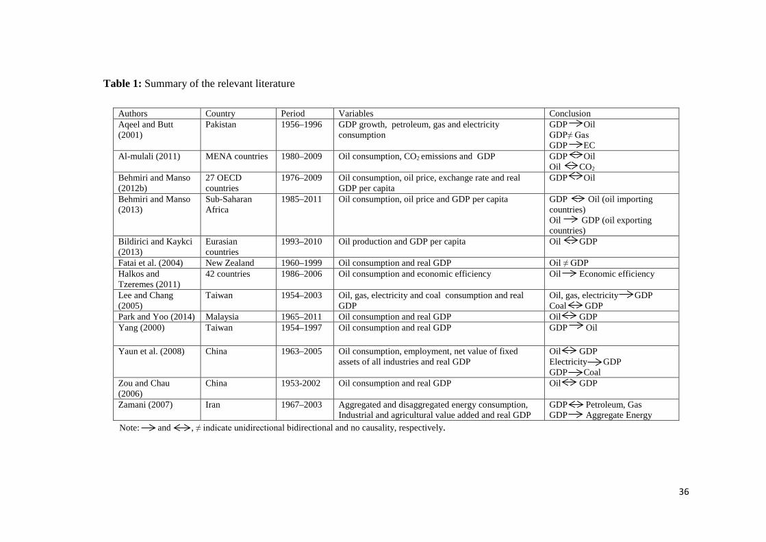
The empirical studies of the causality tests between oil consumption and economic

growth are summarized in Table 1. The assessment of the existing literature review

regarding oil consumption–growth suggests that four kinds of causality exist. First, the

unidirectional causality from oil consumption to economic growth suggests that

increases in oil consumption have a positive effect on economic growth, and a shortage

of oil supply may have an adverse effect on economic growth through production and

transportation. Lee and Chang’s (2005) pioneering study discover unidirectional

causality from oil use to economic growth. Considering Taiwan as a case study, the

7

authors examine the relationship between energy (oil, gas, electricity and coal)

consumption and economic growth between 1954 and 2003. Employing Johansen’s

cointegration test, the study provides empirical evidence that oil consumption leads to

economic growth. The same finding is also revealed in China. He et al. (2005) argue

that both oil consumption and CO2 emissions in China increased significantly due to the

increased demand of oil in the Chinese road transport sector, and predict that both oil

consumption and CO2 emissions will rapidly increase in this sector in the next 25 years.

Furthermore, Halkos and Tzermes (2011) claim that oil consumption helps to increase

economic efficiency in 42 economies across the world.

Second, the unidirectional causality running from economic growth to oil consumption

implies that economic growth increases oil consumption. The rationality to support this

view is that people are expected to consume more oil as their income increases.

Moreover, the use of oil in transportation and production also increases along with

economic growth. These arguments are supported by a number of studies, such as Yang

(2000) and Aqeel and Butt (2001). Yang (2000) investigates the link between oil

consumption and real GDP per capita in Taiwan from 1954 to 1997. The Engle-Granger

causality test yields evidence of unidirectional causality from GDP per capita to oil

consumption. Aqeel and Butt (2001) also report the similar finding in the case of

Pakistan. Their study uses Hsiao’s Granger causality test and finds that economic

growth leads to increase petroleum consumption.

Third, Yaun et al. (2008), Al-mulali (2011), Behmiri and Manso (2012a; 2012b; 2013)

and, Park and Yoo (2014) find a bidirectional causal relationship between oil use and

economic growth. That is, oil consumption and economic growth Granger cause each

8

other and affect simultaneously. In their study, Zou and Chau (2006) investigate the

short- and long-run impacts between oil use and economic growth in China. Using time

series data from 1953 to 2002, the study concludes that oil consumption has a

significant impact on China’s economic growth. In another study on China, Yaun et al.

(2007) explore the causality between energy consumption and economic growth at both

aggregated and disaggregated levels. Employing a neo-classical aggregate production

model, their empirical findings suggest that a bidirectional relationship exists between

oil use and GDP. Zamani (2007) also examines the link between different kinds of

energy and overall GDP, controlling industrial and agricultural output in a case study of

Iran. Using an error correction model (ECM) framework, the study discovers that

petroleum consumption and GDP growth affect each other in the long-run. Al-mulali

(2011) examines the effect of oil consumption on the economic growth and CO2

emissions of MENA countries. From a panel data set for the period 1980–2009, the

study finds that bidirectional causality exists between oil consumption, economic

growth and CO2 emissions.

Another study by Behmiri and Manso (2012a) employ a trivariate framework to explore

the nexus between oil consumption, economic growth and oil prices in Portugal from

1980 to 2009. The study uses both panel cointegration and Granger causality tests and

reports that there is bidirectional causality between oil consumption and economic

growth. The same authors (Behmiri and Manso, 2012b) investigate the same issue in 27

Organization for Economic Cooperation and Development (OECD) countries, and

provide empirical evidence of bidirectional relationship existence both in the short- and

long-run. In a further study, the authors (Behmiri and Manso, 2013) examine the same

9

issue in the major economies of Sub-Saharan Africa during 1985–2011, where they

divide the selected countries into the two major groups of net oil- importing and

exporting countries. The Granger causality test suggests that, in the short-run, there is

bidirectional causality and unidirectional causality from oil use to GDP growth in oil-

importing and exporting countries, respectively. However, there is bidirectional

causality between the variables in both regions in the long-run. More recently, Park and

Yoo (2014) examine the causal relationship between oil consumption and economic

growth in Malaysia where oil use and real GDP has rapidly increased over the last

couple of decades. From ECM models, the study confirms that bidirectional causality

exists between oil consumption and economic growth. Moreover, Bildirici and Kaykci

(2004) also support the existence of bidirectional causality between oil production and

GDP growth in Eurasian countries.

Finally, a few studies report the absence of a causal relationship, which implies that

there is no causality between economic growth and oil consumption. To be specific,

Wolde-Rufael (2004) explores the causal relationship between disaggregate industrial

energy consumption and economic growth in the Chinese province of Shanghai. Using

time series data for the period of 1952 to 1999, the study argues that oil consumption

does Granger cause economic growth and vice versa. Fatai et al. (2004) also make the

same finding in the context of New Zealand. The authors investigate the impact of

various kinds of energy consumption and economic growth in six different countries,

including Australia, New Zealand, India, Indonesia, Thailand, and the Philippines,

covering the period between 1960 and 1999. From Johansen’s cointegration and Toda-

10

Yamamoto causality tests, the study discovers that no Granger causality running in any

direction between oil use and GDP growth in New Zealand.

A number of studies document in the literature that financial development,

industrialization and trade openness can also have a significant impact on energy

consumption and CO2 emissions. First, financial development is the indication of an

efficient stock market and financial intermediation, which gives a platform for listed

companies to lower their cost of capital with increasing financial channels,

disseminating operating risks and optimizing asset/liability structure. This eventually

encourages new installations and investments in new projects that then have a

considerable impact on energy consumption and CO2 emissions. Moreover, the

presence of an efficient financial system leads to more consumer-loan activities, which

indeed makes consumers to buy more energy-consuming products and causes for more

CO2 emissions. These arguments are empirically supported by Jensen (1996) and Zhang

(2011). Jensen (2011) argues that financial development encourages CO2 emissions as it

increases manufacturing production. Employing VECM and variance decomposition

approach, Zhang (2011) finds that financial development significantly increases CO2

emissions and thereby environmental degradation in China.

However, a number of studies reveal a positive relationship between financial

development and environmental quality. For instance, Lanoie et al. (1998) argue that an

efficient financial market provides incentives to its companies/firms to comply with

environmental regulations that help to mitigate environmental degradation. Kumbaroglu

et al. (2008) also support Lanoie et al. (1998) findings by concluding that financial

development helps to significantly reduce CO2 emissions in Turkey by using advanced

11

greener technology in the energy sector. Tamazian et al. (2009) investigate the effect of

economic and financial development on CO2 emissions in some of the most emerging

economies, including Brazil, Russia, India and China (BRIC) nations. Using panel data

over the period 1992–2004, the authors find that both factors are essential for CO2

reductions. Tamazian and Rao (2010) also inspect the impact of financial, institutional

and economic development on CO2 emissions for 24 transitional economies during

1993 to 2004. Using a GMM model, the study reports that financial development helps

lower CO2 emissions by promoting investment in energy efficient sector. However, the

authors point out that financial liberalization may be harmful for environmental quality

if it is not accomplished within a strong institutional framework. Following the ARDL

bound testing procedure; Jalil and Feridun (2011) also present the similar findings using

Chinese aggregate data over the period 1953–2006.

Second, the link between industrialization, energy consumption and CO2 emissions has

become a growing interest among the energy economists and policymakers around the

world. For example, Jones (1991) examines industrialization and energy use. Using data

from developing countries, the study reveals that industrialization increases the

consumption of energy. York et al. (2003) examine the impact of industrialization and

urbanization on the environment and find that both of these factors degrade environment

quality through increasing CO2 emissions. Employing a wide range of data from 99

countries during the 1975–2005 period, Poumanyyoung and Kaneko (2010) find that a

1% increase in industrial output increases 0.069% of energy consumption, a significant

finding for low- and middle-income countries. Using heterogeneous panel regression,

Sadorsky (2013) claims that industrialization increases energy intensity both in the

12

short- and long-run for a panel of 76 developing countries. The same author (Sadorsky,

2014) makes the same finding in the context of emerging economies. Considering

Bangladesh as a case study, Shabaz et al. (2014) examine the relationship between

industrialization, electricity consumption and CO2 emissions. The ARDL bounds

testing approach suggests that the Enviornmental Kuznets curve (EKC) exists between

industrial output and environment. All of these studies argue that industrialization

requires more equipment and machineries to carry out the production of goods and

services, which will then consume more energy and releases higher CO2 emissions than

the traditional agricultural or manufacturing activities.

Finally, trade openness also has a considerable impact on energy consumption. An

increase in exports and imports of goods and services requires more economic activities,

such as production, processing and transportation. These activities will intensify energy

consumption and CO2 emissions. There is an extensive amount of literature, such as

Jena and Grote (2008), Ghani (2012) and Sadorsky (2011, 2012), who claims that trade

openness increases energy consumption. However, only a few studies examine the link

between trade openness and CO2 emissions, with the pioneering study by Grossman and

Krueger (1991). Subsequently, similar research questions have also been examined by a

number of studies, such as Lucas et al. (1992), Wyckoff and Roop (1994), Nahman and

Antrobus (2005), etc. However, all of these earlier studies fail to find conclusive

evidence of the relationships between trade and environmental quality. Halicioglu’s

study (2009), which uses Turkish data, is probably the first to reveal that trade is one

important determinant of CO2 emissions. Hossain (2011) also finds a positive

relationship between trade openness and CO2 emissions in newly industrialized

13

countries. Moreover, Ozturk and Acaravci (2013) also found that foreign trade increases

CO2 emissions in Turkey for the 1960-2007. A recent study by Ren et al. (2014)

examines the impact of international trade on CO2 emissions in China for the period

2000-2010. Based on the two-step GMM estimation, the study argues that China’s trade

surplus is one of the important reasons for the rapidly increasing CO2 emissions.

[Insert Table 1 Here]

The above review suggests that the relationship between oil consumption and economic

growth varies across countries, periods and methods. Moreover, most of the studies

have been conducted on individual Asian countries using time series techniques, and

panel frameworks are scarce. As most of the studies address the causality within an

individual country, their findings cannot be generalised as the results suffer from a short

data span that leads to a reduction of the unit root and cointegration test power. Further,

most of the existing literature focuses on a causal link from a bivariate model and

ignores the dynamic relationship from a multivariate model. Hence, this study is a

modest attempt to address these limitations, and to contribute to the body of knowledge

in this area and provide potential policy implications for sustainable economic growth.

III. Methodology

In this paper, we use panel econometric models for the analysis because of the

numerous advantages it offers in comparison to cross-section and time series models.

For example, a panel data set not only provides more information on the given variables

but also control for individual heterogeneity that exists across cross-sections. This

ultimately increases the efficiency and reliability of the econometric estimation.

14

Additionally, panel data set estimation can assist in overcoming the problems connected

with insufficient distributions and non-stationarity issues that are often experienced in

time series data sets, particularly in the case of shorter duration. The panel econometric

models are based on the following variables: CO2 emissions (CO2E), which is a

function of financial development (FD), economic growth (GDPPC), industrialization

(IND), oil consumption (OILCON) and trade openness (TRDOPN). The basic and

general framework for determinants of CO2 emissions can be written as follows:

),,,,,(2 iitititititit ZTRDOPNOILCONINDGDPPCFDfECO = (1)

Eq. (1) can be parameterized as follows:

iitititititit VTRDOPNOILCONINDGDPPCFDECO iiiii 543212

βββββ= (2)

Eq. (2) can be re-written in a simple regression framework by adding a random error

term as follows:

itiitiitiitiitiitiit ZTRDOPNOILCONINDGDPPCFDECO εβββββ ++++++= )ln()ln()ln()ln()ln()ln( 543212 (3)

In Eq. (3), ln represents the natural logarithms, countries are denoted by the subscript i

),......,1( Ni = , and t denotes the time period ),.......,1( Tt = . This equation is a fairly

general specification, which accounts for individual country fixed effects )(Z and a

stochastic error term )(ε .

Panel unit root tests

In this study, we start with panel unit root tests. Applying unit root tests on a time series

data set has become an important factor for researchers to understand the distributional

15

properties of a data series and also the order of integration of the variables before

applying any econometric model. At the same time, applying unit root tests on a panel

data series is a new phenomenon. Thus, the growing popularity of panel data set among

economists has attracted a great deal of attention towards the application of panel unit

root tests. Further, the results from panel unit root test are more consistent than those of

normal unit root test for an individual time series. Given these advantages, in this study,

we use two panel unit root tests that investigate the common as well as individual unit

root processes on each of the variables. For the former, we employ Breitung (2000) t-

stat test, while the latter is examined using Im et al. (2003) test.

Panel cointegration tests

We apply panel cointegration techniques to explore the long-run equilibrium

relationship between CO2 emissions, economic growth, financial development,

industrialization, oil consumption and trade openness in a sample of 18 emerging

economies. Panel cointegration techniques provide better results than models estimated

from the individual time series. This is due to the fact that the models estimated from

cross-sections of a time series data set have a greater degree of freedom and provide

consistent results. Therefore, we employ three panel cointegration models: a Fisher-type

cointegration test (Maddala and Wu, 1999); the Kao (1999) cointegration test; and the

Pedroni (1999, 2004) cointegration test. The Fisher test is based on the Johansen

combined test while the second (Kao) and third (Pedroni) cointegration tests are based

16

on the Engle and Granger (1987) two-step (residual-based) cointegration approach. The

following section provides a brief description on the above panel cointegration models.2

Fisher-Johansen panel cointegration test. As mentioned above, we aim to explore the

long-run relationship between the given variables. Thus, we start with Fisher-Johansen

panel cointegration test. Fisher (1932) developed a combined test that utilizes the results

of individual independent tests. More recently, Maddala and Wu (1999) apply Fisher’s

test to propose an alternative method for testing a cointegration relationship in a panel

data set by combining tests from individual cross-sections to acquire a test statistic for

the entire panel. The suitable lag length for this test is selected based on the Schwarz

information criterion (SIC). The null hypothesis of no cointegration is tested against the

alternative hypothesis of cointegration. This test can be described with the following

model: if iπ is the p-value from an individual cointegration test for a cross-section i , the

panel under the null hypothesis is:

22

1)log(2 N

N

ii x→− ∑

=

π (4)

where the 2x value is based on the MacKinnon et al. (1999) p-values for Johansen’s

trace and imummax eigenvalue tests.

Kao cointegration (Engle-Granger based) test. The Kao panel cointegration test is

based on Engle and Granger (1987) two-step procedure. This cointegration test clearly

defines intercepts for cross-sections and homogenous coefficients on the first-stage

regressors. The Kao (1999) has described the bivariate regression model as follows: 2 Due to space limitation, detailed equations and a detailed discussion of the panel cointegration models are excluded.

17

ititiit xy εβα ++= (5)

tiitit yy ,1 υ+= − (6)

tiitit exx ,1 += − (7)

where y and x are assumed to be integrated of order one, i.e., I (1), and i and t denote

country and time period, respectively. The first-stage regression can be carried out using

Eq. (5) where iα is heterogeneous, iβ is homogenous across cross-sections, and itε is

the residual term. This cointegration test utilizes an augmented version of the Dickey-

Fuller test for testing the null hypothesis of no cointegration against the alternative

hypothesis of cointegration. The appropriate lag length for this test is chosen based on

the SIC.

Pedroni cointegration (Engle-Granger based) test. The Pedroni (1999, 2004) panel

cointegration test is also based on Engle and Granger (1987) two-step procedure. The

Pedroni test provides seven statistics for tests of the null hypothesis of no cointegration

in heterogeneous panels. These seven statistics can be classified into two parts: the first

four statistics represent within-dimension (panel tests) and the last three statistics

constitute between-dimension (group tests). These seven tests are performed based on

the residuals from Eq. (3). The null hypothesis of no cointegration ( =iρ 1 for all i ) is

tested against the alternative hypothesis of 1<= ρρ i for all i for the within-dimension.

Likewise, in the case of the group-means approach, it is less restrictive because it does

not need a common value of ρ under the alternative. Therefore, for the group-means

approach, the alternative hypothesis is ii <ρ for all i . As we discussed above, the

between-dimension tests are less restrictive; therefore, they allow for heterogeneous

18

parameters across the cross-sections. The lag length for this test is selected based on the

SIC.

Panel Granger causality test

In this section, we describe the methodology that aims to explore the dynamic causal

relationship between CO2 emissions, economic growth, financial development,

industrialization, oil consumption and trade openness. Engle and Granger (1987) argue

that if non-stationary variables are cointegrated in the long-run, then the vector error

correction model (VECM) can be applied for exploring the direction of causality among

the variables in the short-run as well as in the long-run. The short-run Granger causality

can be established by conducting a joint test of the coefficients based on the F-test and

the 2x test. Likewise, the long-run Granger causality between the variables can be

understood through the statistical significance of the lagged error term in the VECM

framework based on the t-statistics.

The panel Ganger causality test for short-run and long-run can be described based on

the following equations:

itit

K

iitit

K

iitit

K

iitit

K

iitit

K

iitit

K

iititititit TRDOPNOILCONINDGDPPCFDECOectECO µθγϕφδϑβα ++∆+∆+∆+∆+∆++=∆ −

=−

=−

=−

=−

=−

=− ∑∑∑∑∑∑ 1

11

11

11

11

112

112 (8)

itit

K

iitit

K

iitit

K

iitit

K

iitit

K

iitit

K

iititititit TRDOPNOILCONINDGDPPCECOFDectFD µθγϕφδϑβα ++∆+∆+∆+∆+∆++=∆ −

=−

=−

=−

=−

=−

=− ∑∑∑∑∑∑ 1

11

11

11

112

11

11 (9)

itit

K

iitit

K

iitit

K

iitit

K

iitit

K

iitit

K

iititititit TRDOPNOILCONINDFDECOGDPPCectGDPPC µθγϕφδϑβα ++∆+∆+∆+∆+∆++=∆ −

=−

=−

=−

=−

=−

=− ∑∑∑∑∑∑ 1

11

11

11

112

11

11

(10)

itit

K

iitit

K

iitit

K

iitit

K

iitit

K

iitit

K

iititititit TRDOPNOILCONGDPPCFDECOINDectIND µθγϕφδϑβα ++∆++∆+∆+∆++=∆ −

=−

=−

=−

=−

=−

=− ∑∑∑∑∑∑ 1

11

11

11

112

11

11 (11)

19

itit

K

iitit

K

iitit

K

iitit

K

iitit

K

iitit

K

iititititit TRDOPNINDGDPPCFDECOOILCONectOILCON µθγϕφδϑβα ++∆+∆+∆+∆+∆++=∆ −

=−

=−

=−

=−

=−

=− ∑∑∑∑∑∑ 1

11

11

11

112

11

11

(12)

itit

K

iitit

K

iitit

K

iitit

K

iitit

K

iitit

K

iititititit OILCONINDGDPPCFDECOTRDOPNectTRDOPN µθγϕφδϑβα ++∆+∆+∆+∆+∆++=∆ −

=−

=−

=−

=−

=−

=− ∑∑∑∑∑∑ 1

11

11

11

112

11

11

(13)

where ∆ is the first difference operator, itα is the constant term, itititititit γϕφδϑβ ,,,,,

and itθ are the parameters, 1−itect is the error correction term obtained from the VECM

models, k is the lag length and itµ is the white-noise error term.

IV. Data and Preliminary Statistics

Nature of data and measurement

The study uses a balanced panel data set of 18 emerging economies across the world

from 1980 to 2012. The considered countries in the sample are as follows: Algeria

(ALG), Argentina (ARG), Brazil (BRA), China (CHI), Colombia (COL), Egypt (EGY),

India (IND), Indonesia (INDO), Iran (IRA), Malaysia (MAL), Mexico (MEX), Nigeria

(NIG), Pakistan (PAK), the Philippines (PHI), South Africa (SOU), Thailand (THA),

Turkey (TUR) and Venezuela (VEN). The countries are selected according to the

following two criteria; first, the country should consume at least 200,000 barrels of

petroleum per day on average from 1980 to 2012; second, the country should have a

developing economy.3 Annual data on CO2 emissions, economic growth, financial

development, industrialization, oil consumption and trade openness is employed.

3 All developed countries (as defined by the World Bank) are excluded from the analysis, because developing countries often contribute higher CO2 emissions, which eventually degrade the environment. Hence, we aim to understand the major contributors of CO2 emissions in developing countries and provide potential policy implications for mitigating CO2 emissions and sustainable economic growth.

20

The measurement of the variables are as follows: CO2 emissions are measured per

capita metric tons (CO2E); economic growth is captured by real GDP per capita

(GDPPC, constant 2005 US$); financial development (FD) is measured by domestic

credit to private sector as a share of GDP; industrialization (IND) is measured using

total value added by the industry as a share of GDP; per capita petroleum consumption

(litres) is used as a proxy for oil consumption; and trade openness (TRDOPN) is

measured by the sum of exports and imports (goods and services) as a share of GDP.

Data on petroleum consumption is collected from EIA while data on CO2E, FD,

GDPPC, IND and TRDOPN are collected from the World Development Indicators’

(WDI) online data source (World Bank). We transformed all the variables into natural

logarithms before estimating any economic models, since log-linear specification can

produce better results than the linear functional form of the model.

Time-series trend of CO2 emissions, oil consumption and per capita GDP

Fig. 1 shows time series plots of per capita CO2 emissions (metric tons) for each of the

countries. Overall, CO2 emissions increased over time for all countries except Nigeria.

On average, South Africa, Venezuela, Iran and Malaysia have the highest per capita

CO2 emissions, while Nigeria, Pakistan and the Philippines have the lowest. The graphs

also reveal that Algeria, Argentina, Colombia, Mexico, Nigeria, the Philippines, South

Africa and Venezuela observed a sharp volatile growth in CO2 emissions over the last

three decades, while China, India, Pakistan, Thailand and Turkey experienced steady

growth.

[Insert Fig.1 Here]

21

Fig. 2 exhibits time series graphs of per capita oil consumption (liters) for each of the

selected emerging economies. These graphs suggest that oil consumption experienced

an upward trend for all of the countries, except Colombia, Mexico, Nigeria and the

Philippines. However, the strength of the trend differs significantly from one country to

another. These graphs indicate that, on average, Venezuela, Iran and Mexico have the

highest per capita oil consumption, while India, Pakistan, Nigeria, China and the

Philippines have the lowest. Over the last three decades, the per capita oil consumption

in China, India and Indonesia is steadily increasing.

[Insert Fig.2 Here]

Fig. 3 presents the time series plots of real GDP per capita (constant 2005, US$) for

each of the selected countries. The graphs show that all of the countries enjoyed positive

GDP (per capita) growth over the time period. The graph indicates that Mexico, Turkey,

Venezuela and South Africa have the highest per capita GDP, while India, Pakistan and

Nigeria have the lowest. Moreover, the GDP per capita growth in China, Egypt, India,

Indonesia, Malaysia, Pakistan, and Turkey was impressive as these countries enjoyed

steady growth across time. Further, the figures indicate that, during 2007 to 2009, China

and India were affected the least by the global financial crisis, while Mexico, Turkey

and Venezuela were affected the most.

[Insert Fig.3 Here]

22

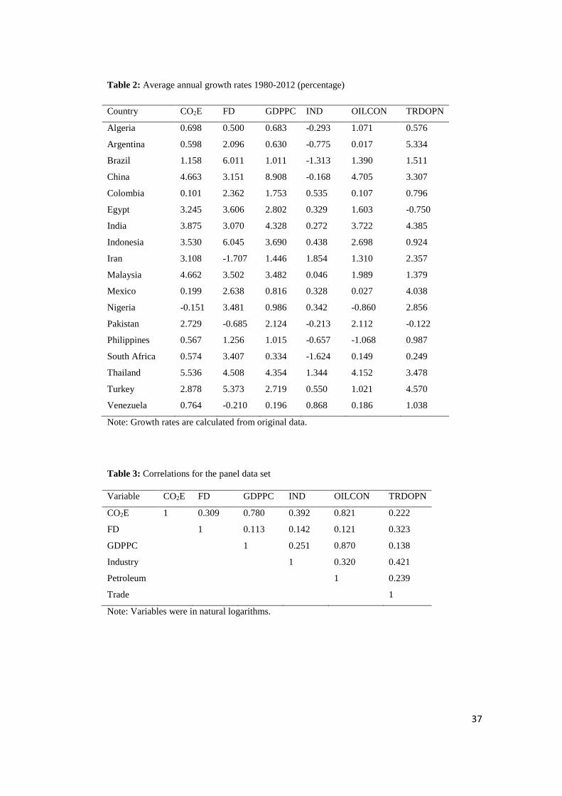
Average annual growth rates

Table 2 displays the average annual growth rates for all the countries during the period

1980 to 2012 as percentages.4 All of the selected countries experienced increased CO2

emissions, except for Nigeria (-0.15%). Thailand (5.54%), China (4.6%) and Malaysia

(4.6%) had the highest growth rates of CO2 emissions, while Colombia and Mexico had

the lowest growth rate. The highest financial development growth was recorded in

Indonesia (6.05%), Brazil (6.01%) and Turkey (5.37%), while Iran (-1.71%), Pakistan (-

0.69%) and Venezuela (-0.21%) experienced negative growth. At the same time,

Thailand (4.51%), Egypt (3.61%), Malaysia (3.5%), Nigeria (3.48%), South Africa

(3.41%), China (3.15%) and India (3.07%) experienced moderate growth. Average

growth rates for GDP per capita indicate that China was the leader by far (8.91%),

followed by Thailand (4.35%) and India (4.33%). However, the growth of GDP per

capita in Venezuela (0.20%), South Africa (0.33%), Argentina (0.63%) and Algeria

(0.68%) were the lowest among the selected countries. The industrial growth rates show

that Iran (1.85%) and Thailand (1.34%) have greater growth, while South Africa (-

1.62%), Brazil (-1.31%), Argentina (-0.78%), the Philippines (-0.66%), Pakistan (-

0.21%) and China (-0.17%) experienced negative growth.

The highest average growth rates of per capita oil consumption belong to China

(4.71%), Thailand (4.15%) and India (3.72%), while Nigeria (-0.86) and the Philippines

(-1.07%) had the lowest growth rates. Finally, the growth rates for trade openness

suggest that the selected countries can be classified into four groups. The first one

enjoyed rapid growth, maintaining more than 3% average growth rates, includes 4 Growth rates are calculated using original data (before converting into natural logarithms).

23

Argentina (5.33%), Turkey (4.57%), India (4.39%), Mexico (4.03%), Thailand (3.48%)

and China (3.31%). The second group observed modest growth rates ranging from 1%

to 3% namely Nigeria (2.86%), Iran (2.36%), Brazil (1.51%), Malaysia (1.38%),

Venezuela (1.04%), the Philippines (0.99 or 1%) and Indonesia (0.92 or 1%). The third

group had experienced very low but positive growth rates such as Colombia (0.79%),

Algeria (0.58%) and South Africa (0.25%). Lastly, the fourth group covers two

economies, Pakistan (-0.12%) and Egypt (-0.75%), who experienced negative growth.

[Insert Table 2 Here]

Unconditional correlations among the variables

The unconditional correlations5 between the panel data variables are presented in Table

3. This table reflects that CO2 emissions have the highest correlation with oil and GDP

per capita and the lowest correlation with trade openness. Financial development has the

strongest relationship with trade openness and CO2 emissions and the weakest

relationship with GDP per capita. Likewise, GDP per capita is significantly correlated

with oil and CO2 emissions and least correlated with financial development. The highest

correlation for oil consumption is with GDP per capita and CO2 emissions, while the

lowest correlation is with FD. Finally, trade openness has a moderate correlation with

all variables except GDP per capita. The most significant point that can be ascertained

from Table 3 is that oil consumption is strongly correlated with GDP per capita and CO2

emissions, which suggests that the consumption of oil increases both GDP per capita

and CO2 emissions, and vice versa. A similar link is also revealed in the case of real

5 Unconditional correlations are calculated using data in natural logarithms.

24

GDP per capita and CO2 emissions where these two variables have the highest

correlations with oil consumption and between them. This therefore indicates that these

three variables have a significant relationship in selected economies.

[Insert Table 3 Here]

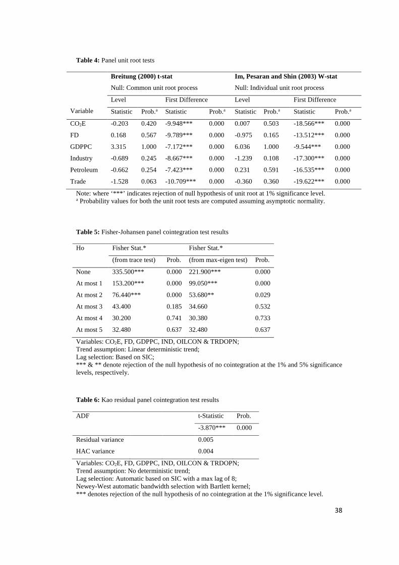
Results of unit root tests

In this paper, we employ two panel unit root tests that examine both common as well as

individual unit root processes. For example, the Breitung (2000) test examines the null

hypothesis of common unit root process against the alternative hypothesis of no unit

root. Similarly, the Im et al. (2003) test examines the null hypothesis of individual unit

root processes across the cross sections against the alternative hypothesis of some cross-

sections do not have a unit root. The results of these two unit root tests are presented in

Table 4. The results at levels for both the tests show that the null hypothesis of a unit

root (common as well as individual) cannot be rejected at the 1% or 5% significance

levels for all the given variables. However, at first difference, the null hypothesis of unit

root can be rejected at the 1% significance level for all of the variables. Hence, our

results confirm that all of the variables have a unit root process at levels and are

stationary at their first order differences. This indicates that all of the variables are

integrated of order I (1).

[Insert Table 4 Here]

25

V. Empirical Results and Discussion

The aim of this section is to empirically investigate the long-run equilibrium

relationship between CO2E, FD, GDPPC, IND, OILCON and TRDOPN using three

robust panel cointegration techniques. Further, we explore the short-run and long-run

dynamic causal relationship between these variables using the VECM approach. The

empirical results of these models are presented and discussed below.

Results of cointegration tests

The results of two unit root tests confirm that CO2 emissions, financial development,

economic growth, industrialization, oil consumption, and trade openness are non-

stationary at their levels, and stationary at their first order differences. Therefore, these

unit root tests results indicate that a long-run equilibrium relationship may exist

between all of these variables. Hence, we apply cointegration models to explore the

long-run cointegration relationship between the dependent variable (CO2E) and the

independent variables (FD, GDPPC, IND, OILLCON and TRDOPN). As previously

discussed, in this study, we employ three robust panel cointegration techniques: the

Fisher-type test using the approach developed by Johansen (Maddala and Wu, 1999),

the Kao (1999) test, and finally the Pedroni (1999, 2004) test. The empirical results of

these cointegration techniques are presented below.

The results of the Johansen-Fisher panel cointegration test are reported in Table 5. This

test requires using an appropriate lag length for the analysis. We therefore select the

suitable lag length for this test based on the SIC and we also confirmed that the selected

lag length residuals are random. The results of this test on both the trace and maximum

26

eigen tests suggest that the null hypothesis of no cointegration is rejected at the 5%

significance level. This therefore indicates that the variables of FD, GDPPC, IND,

OILCON and TRDOPN are strongly cointegrated with CO2E. Our results confirm that

these variables share a long-run equilibrium relationship in the case of major oil-

consuming emerging economies of the world.

[Insert Table 5 Here]

Likewise, we explore the long-run relationship between the same variables using the

methodology developed by Kao (1999), the results of which are displayed in Table 6.

This test, based on the Engle-Granger approach, is similar to Pedroni (1999, 2004)

cointegration test; however, it defines specific cross-section intercepts and homogenous

coefficients on the first stage of regressors. This cointegration test also requires an

appropriate lag length for the analysis, which we select based on the SIC. The results of

this test reveal that the null hypothesis of no cointegration is rejected at the 1%

significance level. These results suggest that there is a long-run equilibrium relationship

between CO2E, FD, GDPPC, IND, OILCON and TRDOPN.

[Insert Table 6 Here]

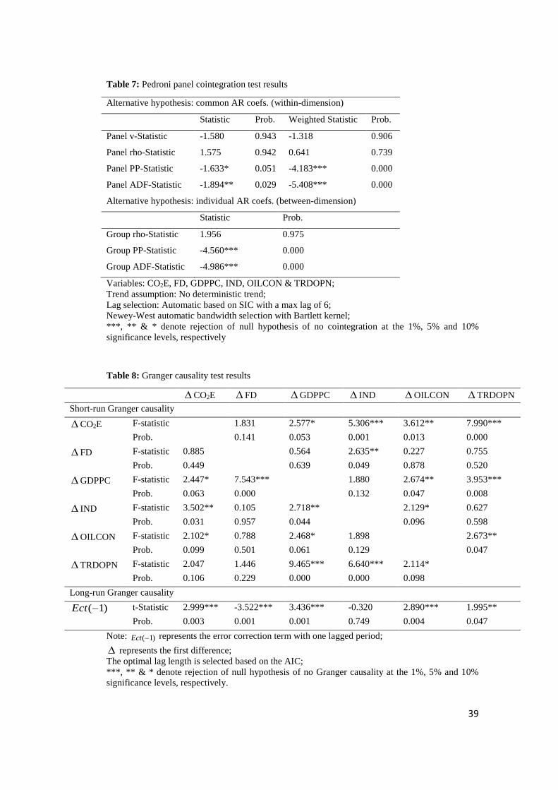
Finally, we apply the Pedroni (1999, 2004) panel cointegration test to investigate the

long-run relationship between the given variables, and the empirical results are reported

in Table 7. The Pedroni cointegration test is also based on the Engle-Granger approach.

To perform the Pedroni cointegration test, first we have to identify the suitable lag

length, which is chosen based on the SIC and it is also confirmed that the residuals of

selected lag length are random. The results of Pedroni test show that out of the seven

27

statistics, two statistics (within-dimension) reject the null hypothesis of no cointegration

at the 10% and 5% level of significances, respectively. At the same time, two statistics

(between-dimension) reject the null hypothesis of no cointegration at the 1%

significance level. The results of Pedroni cointegration test on both within and between

dimensions confirm that there is a long-run equilibrium relationship between CO2E, FD,

GDPPC, IND, OILCON and TRDOPN in emerging economies. Overall, our three panel

cointegration tests results indicate that there is substantial evidence of a long-run

relationship between the studied variables.

[Insert Table 7 Here]

Results of dynamic short-run and long-run causal relationship

We aim to empirically investigate the dynamic short-run and long-run causal

relationship between CO2E, FD, GDPPC, IND, OILCON and TRDOPN. To achieve

this, we follow the two-step approach developed by Engle-Granger (1987). This

methodology is based on the VECM framework. The lag length for this model is

selected based on the Akaike information criterion (AIC), which ensures that the

residuals of the chosen lag length are random. For the purpose of interpretation and

discussion of these results, we use 1%, 5% and 10% significance levels. Our primary

variables of interest in this study are CO2 emissions, economic growth and oil

consumption. The dynamic Granger causality tests results on short-run and long-run are

presented in Table 8. The short-run Granger causality results display that there is an

evidence of a feedback relationship between CO2 emissions–economic growth and CO2

emissions–oil consumption. Similarly, there is bidirectional causality between economic

28

growth–oil consumption and economic growth–trade openness. We also found

unidirectional causality that runs from industrialization to economic growth. Finally, oil

consumption has a feedback relationship with CO2 emissions, economic growth and

trade openness. Oil consumption is also driven by industrialization.

The short-run Granger causality results suggest that significant growth in economic

expansion and oil consumption leads to higher CO2 emissions in emerging economies.

This indicates that as the economies of those countries grow, their economic activities

will significantly increase consumption of oil which will eventually lead to more and

more CO2 emissions. Thus, CO2 emissions have a positive impact on economic growth,

industrialization, oil consumption and trade openness. In the short-run, increase in CO2

emissions has several positive indications; however, it is going to be a major concern in

the long-term. Therefore, policymakers and environmental scientists have to work out

clearly on minimizing the CO2 emissions, particularly in emerging countries. The

reason being is that in emerging countries both policymakers and government officials

are more concerned about the economic problems such as, poverty and unemployment

than the environmental problems.

The results on long-run (error correction term) causality shows that CO2 emissions,

economic growth, financial development, oil consumption and trade openness have

bidirectional causality. These long-run causality results suggest that the economic

expansion of emerging economies is heavily dependent on the functioning and

contributions of financial development, oil consumption, exports and imports of goods

and services and CO2 emissions. Similarly, the consumption of oil is also largely

dependent on financial development, economic growth and the role of international

29

trade. Overall, our results on short-run and long-run causality suggest that there is a

significant dynamic causal relationship between CO2 emissions, economic growth and

oil consumption in emerging economies. The results of long-run causalities are

consistent with those found by Al-mulali (2011) and Behmiri and Manso (2012b).

[Insert Table 8 Here]

VI. Conclusion

A number of previous studies examine the nexus between energy consumption–

economic growth, energy consumption–industrialization and energy consumption–

financial development. However, a small amount of literature exists on the impact of

economic growth, financial development, industrialization, trade openness and energy

consumption on CO2 emissions. Additionally, the previous studies have failed to

consider the impact of oil consumption on CO2 emissions by taking economic growth,

financial development and industrialization and trade openness into account.

Furthermore, the previous studies have not explored the linkage between these

variables, particularly in the case of major oil-consuming emerging economies.

Therefore, in this study we aim to examine the impact of economic growth, financial

development, industrialization, oil consumption and trade openness on the CO2

emissions of a panel of 18 major oil-consuming emerging economies.

The empirical results of three panel cointegration models suggest that a significant long-

run equilibrium relationship exists between economic growth, financial development,

industrialization, oil consumption, trade openness and CO2 emissions. This evidence

indicates that all of these variables share a common trend in the long-run. Furthermore,

30

results from short-run Granger causality test display a dynamic feedback relationship

between economic growth, oil consumption and CO2 emissions. Similarly, the results

also show bidirectional causality between economic growth and trade openness and

unidirectional causality from industrialization to economic growth. In addition, oil

consumption also has bidirectional causality with trade openness and unidirectional

causality from industrialization to oil consumption. Further, the results indicate that CO2

emissions, economic growth, financial development, oil consumption and trade

openness have a bidirectional causal relationship in the long-run (error correction term).

The results on both the short-run and long-run causality indicate that significant growth

in economic activities and oil consumption leads to larger CO2 emissions in emerging

economies. These results suggest that as the economies of those countries grow, their

economic activities will lead to increase oil consumption, which will ultimately release

a significant amount of CO2 emissions into the atmosphere. Our evidence shows that

CO2 emissions have a positive impact on economic growth, industrialization, oil

consumption and trade openness in the short-run. This argument for the short-run

suggests that an increase in CO2 emissions has a positive impact on the creation of

wealth and opportunities. However, it may be a major concern in the long-term if a

significant amount of attention is not paid to this issue. Therefore, we suggest that

policymakers and environmental scientists of those emerging countries work towards

minimizing CO2 emissions. It is understood that both policymakers and government

officials in emerging economies are often more concerned about the economic problems

that their countries are facing, such as poverty and unemployment, than the long-term

effects of CO2 emissions.

31

The major inferences of this study are as follows. A significant amount of CO2

emissions is caused by increased economic activities and oil consumption. This has

important policy implications for energy and environmental policies. The economic

policies designed for expanding economic activities will increase oil consumption and

lead to higher CO2 emissions. If the predictions for future economic expansion are made

without considering the supply and demand for oil, then the expected economic growth

rates may not be met. Further, we argue that the consumption of oil has a severe impact

on the environment, therefore policymakers and environmental scientists should

develop policies to promote the use of renewable resources rather than non-renewable

resources like oil. Furthermore, environmental policies that are designed for reducing

oil consumption will adversely affect economic growth. Hence, better energy and

environmental policies have to be designed in such a way that they will facilitate an

increase in demand for energy consumption by increasing the share of renewable energy

resources. As discussed above, our study offers significant contributions to the body of

knowledge on the context of CO2 emissions, economic growth and oil consumption,

particularly in the perspective of major oil-consuming emerging economies and has

important policy implications to mitigate environmental degradation and ensure

sustainable economic development.

32

Refferences

Akinlo, A. E. (2008) Energy consumption and economic growth:evidence from 11 Sub-Sahara African countries, Energy Economics, 30, 2391-400.

Alam, M. J., Begum, I. A., Buysse, J., Rahman, S.and Van Huylenbroeck, G. (2011) Dynamic modeling of causal relationship between energy consumption, CO2 emissions and economic growth in India, Renewable and Sustainable Energy Reviews, 15, 3243-51.

Al-Mulali, U. (2011) Oil consumption, CO2 emission and economic growth in MENA countries, Energy, 36, 6165-71.

Apergis, N., Payne, James E., Menyah, K. and Wolde-Rufael, Y. (2010) On the causal dynamics between emissions, nuclear energy, renewable energy, and economic growth, Ecological Economics, 69, 2255-60.

Aqeel, A. and Butt, Mohammad S. (2001) The relationship between energy consumption and economic growth in Pakistan, Asia-Pacific Development Journal, 8, 101-10.

Behmiri, N. B and Manso, J. R. P. (2012a) Does Portuguese economy support crude oil conservation hypothesis?, Energy Policy, 45, 628-34.

Behmiri, N. B and Manso, J. R. P. (2012b) Crude oil conservation policy hypothesis in OECD (organisation for economic cooperation and development) countries: A multivariate panel Granger causality test, Energy, 43, 253-60.

Behmiri, N. B and Manso, J. R. P. (2013) How crude oil consumption impacts on economic growth of Sub-Saharan Africa?, Energy, 54, 74-83.

Bildirici, M. E. and Bakirtas, T. (2014) The relationship among oil, natural gas and coal consumption and economic growth in BRICTS (Brazil, Russian, India, China, Turkey and South Africa) countries, Energy, 65, 134-44.

Bildirici, M. E. and Kayıkçı, F. (2013) Effects of oil production on economic growth in Eurasian countries: Panel ARDL approach, Energy, 49, 156-61.

BP (2007) The BP Statistical Review of World Energy. British Petroleum, London, UK. Avialbale at http://www.bp.com/statistical.review.

Breitung, J. (2000) The local power of some unit root tests for panel data, in Baltagi, B. (ed.), Advances in Econometrics, 15, 161–178: Nonstationary Panels, Panel Cointegration, and Dynamic Panels, Amsterdam: JAI Press.

Chu, H.-P. and Chang, T. (2012) Nuclear energy consumption, oil consumption and economic growth in G-6 countries: Bootstrap panel causality test, Energy Policy, 48, 762-69.

Dickey, D. A. and Fuller, W. A. (1979) Distribution of the estimators for autoregressive time series with a unit root, Journal of the American statistical association, 74, 427-31.

EIA (2014). Analysis and Projections. U.S. Energy Information Administration, Washington, DC. U.S. Available at http://www.eia.gov/forecasts/steo/report.

Engle, R. F. and Granger, C.W.J. (1987) Co-integration and error correction: representation, estimation, and testing, Econometrica: journal of the Econometric Society, 251-76.

Fisher, I. (1932) Booms and depressions: some first principles, Adelphi Company, New York. Ghani, G. M. (2012) Does trade liberalization effect energy consumption?, Energy Policy, 43, 285-

90. Ghosh, S. (2010) Examining carbon emissions economic growth nexus for India: A multivariate

cointegration approach. Energy Policy, 38, 3008-14. Grossman, G. M. and Krueger, A. B. (1991) Environmental impacts of a North American free trade

agreement: National Bureau of Economic Research. Halicioglu, F. (2009) An econometric study of CO2 emissions, energy consumption, income and

foreign trade in Turkey, Energy Policy, 37, 1156-64. Halkos, G. E. and Tzeremes, N. G. (2011) Oil consumption and economic efficiency: A comparative

analysis of advanced, developing and emerging economies, Ecological Economics, 70, 1354-62.

33

Hamit-Haggar, M. (2012) Greenhouse gas emissions, energy consumption and economic growth: A panel cointegration analysis from Canadian industrial sector perspective, Energy Economics, 34, 358-64.

He, K., Huo, H., Zhang, Q., He, D., An, F., Wang, M. and Walsh, M. P. (2005) Oil consumption and CO2 emissions in China's road transport: current status, future trends, and policy implications, Energy policy, 33, 1499-507.

Hossain, S. (2011) Panel estimation for CO2 emissions, energy consumption, economic growth, trade openness and urbanization of newly industrialized countries, Energy Policy, 39, 6991-99.

IEA (2013) IEA Statistics. International Energy Agency, Paris, France. Available at http://www.iea.org/publications/freepublications/publication/co2emissionsfromfuelcombustionhighlights2013.pdf

Im, K.S., Pesaran, M. H. and Shin, Y. (2003) Testing for unit roots in heterogeneous panels, Journal of econometrics, 115, 53-74.

Jalil, A. and Feridun, M. (2011) The impact of growth, energy and financial development on the environment in China: A cointegration analysis, Energy Economics, 33, 284-91.

Jena, P. R, and Grote, U. (2008) Growth-trade-environment nexus in India, In: Proceedings of the German Development Economics Conference, Zurich.

Jensen, V. (1996). The pollution haven hypothesis and the industrial flight hypothesis: some perspectives on theory and empirics, Working Paper 5, Centre for Development and the Environment, University of Oslo.

Jones, D. W. (1991) How urbanization affects energy-use in developing countries, Energy Policy, 19, 621-30.

Kao, C. (1999) Spurious regression and residual-based tests for cointegration in panel data, Journal of econometrics, 90, 1-44.

Koch, N. (2014) Dynamic linkages among carbon, energy and financial markets: a smooth transition approach, Applied Economics, 46, 715-29.

Kumbaroğlu, G., Karali, N. and Arıkan, Y. (2008) CO2, GDP and RET: An aggregate economic equilibrium analysis for Turkey, Energy Policy, 36, 2694-708.

Lanoie, P., Laplante, B. and Roy, M. (1998) Can capital markets create incentives for pollution control?, Ecological Economics, 26, 31-41.

Lean, H. H, and Smyth, R. (2010) CO2 emissions, electricity consumption and output in ASEAN, Applied Energy, 87, 1858-64.

Lee, C-C. and Chang, C.-P. (2005) Structural breaks, energy consumption, and economic growth revisited: evidence from Taiwan, Energy Economics, 27, 857-72.

Loizides, J. and Vamvoukas, G. (2005) Government expenditure and economic growth: evidence from trivariate causality testing, Journal of Applied Economics, 8, 125-52.

Lucas, G, W. N. and Hettige, R. (1992) The inflexion point of manufacture industries: international trade and environment, World Bank discussion paper(148).

Lütkepohl, H. (1982) Non-causality due to omitted variables, Journal of Econometrics, 19, 367-78 Maddala, G. S. and Wu, S. (1999) A comparative study of unit root tests with panel data and a new

simple test, Oxford Bulletin of Economics and statistics, 61, 631-52. MacKinnon, J.G., Haug, A.A. and Michelis, L. (1999) Numerical distribution functions of likelihood

ratio tests for cointegration, Journal of Applied Econometrics, 14, 563–57. Mehrara, M. (2007) Energy consumption and economic growth: the case of oil exporting countries,

Energy policy, 35, 2939-45. Menyah, K. and Wolde-Rufael, Y. (2010) CO2 emissions, nuclear energy, renewable energy and

economic growth in the US, Energy Policy, 38, 2911-15. Nahman, A. and Antrobus, G. (2005) Trade and the environmental Kuznets curve: is Southern Africa

a pollution haven?, South African journal of economics, 73, 803-14.

34

Ozturk, I. and Acaravci, A. (2013) The long-run and causal analysis of energy, growth, openness and financial development on carbon emissions in Turkey, Energy Economics, 36, 262-67.

Pao, H-T. and Tsai, C.-M. (2010) CO2 emissions, energy consumption and economic growth in BRIC countries, Energy policy, 38, 7850-60.

Park, S.-Y, & Yoo, S.-H. (2014) The dynamics of oil consumption and economic growth in Malaysia, Energy Policy, 66, 218-23.

Pedroni, P. (1999) Critical values for cointegration tests in heterogeneous panels with multiple regressors, Oxford Bulletin of Economics and statistics, 61, 653-70.

Pedroni, P. (2004) Panel cointegration: asymptotic and finite sample properties of pooled time series tests with an application to the PPP hypothesis, Econometric theory, 20, 597-25.

Poumanyvong, P. and Kaneko, S. (2010) Does urbanization lead to less energy use and lower CO2 emissions? A cross-country analysis, Ecological Economics, 70, 434-44.

Ren, S. Yuan, B., Ma, X. and Chen, X. (2014) International trade, FDI (foreign direct investment) and embodied CO2 emissions: A case study of Chinas industrial sectors, China Economic Review, 28, 123-34.

Sadorsky, P. (2010) The impact of financial development on energy consumption in emerging economies, Energy Policy, 38, 2528-35.

Sadorsky, P. (2011) Trade and energy consumption in the Middle East, Energy Economics, 33, 739-49.

Sadorsky, P. (2012) Energy consumption, output and trade in South America, Energy Economics, 34, 476-88.

Sadorsky, P. (2013) Do urbanization and industrialization affect energy intensity in developing countries?, Energy Economics, 37, 52-59.

Sadorsky, P. (2014) The effect of urbanization and industrialization on energy use in emerging economies: Implications for sustainable development, American Journal of Economics and Sociology, 73, 392-409.

Shahbaz, M., Salah Uddin, G., Ur Rehman, I. and Imran, K. (2014) Industrialization, electricity consumption and CO2 emissions in Bangladesh, Renewable and Sustainable Energy Reviews, 31, 575-86.

Soytas, U. and Sari, R. (2009) Energy consumption, economic growth, and carbon emissions: challenges faced by an EU candidate member, Ecological economics, 68, 1667-75.

Stern, D.I. (1993) Energy and economic growth in the USA: a multivariate approach, Energy Economics, 15, 137-50.

Tamazian, A., Chousa, Juan P. and Vadlamannati, K. C. (2009) Does higher economic and financial development lead to environmental degradation: evidence from BRIC countries, Energy Policy, 37, 246-53.

Tamazian, A. and Bhaskara R. B. (2010) Do economic, financial and institutional developments matter for environmental degradation? Evidence from transitional economies, Energy Economics, 32, 137-45.

Tsani, S. Z. (2010) Energy consumption and economic growth: a causality analysis for Greece, Energy Economics, 32, 582-90.

Wolde-Rufael, Y. (2004) Disaggregated industrial energy consumption and GDP: the case of Shanghai, 1952–1999, Energy economics, 26, 69-75.

Wolde-Rufael, Y. and Menyah, K. (2010) Nuclear energy consumption and economic growth in nine developed countries, Energy Economics, 32,550-56.

Wyckoff, A.W. and Roop, J.M. (1994), The embodiment of carbon in imports of manufactured products: Implications for international agreements on greenhouse gas emissions, Energy policy, 22, 187-94.

Yoo, S.-H. (2006) Oil consumption and economic growth: evidence from Korea, Energy Sources, 1,235-43.

35

York, R., Rosa, E.A. and Dietz, T. (2003) STIRPAT, IPAT and ImPACT: analytic tools for unpacking the driving forces of environmental impacts, Ecological economics, 46, 351-65.

Yang, H.-Y. (2000) A note on the causal relationship between energy and GDP in Taiwan, Energy Economics, 22, 309-17.

Yuan, J., Zhao, C., Yu, S., and Hu, Z. (2007) Electricity consumption and economic growth in China: cointegration and co-feature analysis, Energy Economics, 29, 1179-91.

Yuan, J.-H, Kang, J.-G, Zhao, C.-H and Hu, Z.-G. (2008) Energy consumption and economic growth: evidence from China at both aggregated and disaggregated levels, Energy Economics, 30, 3077-94.

Zamani, M. (2007) Energy consumption and economic activities in Iran, Energy Economics, 29, 1135-40.

Zhang, X.-P. and Cheng, X.-M. (2009) Energy consumption, carbon emissions, and economic growth in China, Ecological Economics, 68, 2706-12.

Zhang, Y.-J. (2011). The impact of financial development on carbon emissions: An empirical analysis in China, Energy Policy, 39, 2197-203.

Zou, G. and Chau, K.W. (2006) Short-and long-run effects between oil consumption and economic growth in China, Energy Policy, 34, 3644-655.

36

Table 1: Summary of the relevant literature

Authors Country Period Variables Conclusion Aqeel and Butt (2001)

Pakistan 1956–1996 GDP growth, petroleum, gas and electricity consumption

GDP Oil GDP≠ Gas GDP EC

Al-mulali (2011) MENA countries 1980–2009 Oil consumption, CO2 emissions and GDP GDP Oil Oil CO2

Behmiri and Manso (2012b)

27 OECD countries

1976–2009 Oil consumption, oil price, exchange rate and real GDP per capita

GDP Oil

Behmiri and Manso (2013)

Sub-Saharan Africa

1985–2011 Oil consumption, oil price and GDP per capita GDP Oil (oil importing countries) Oil GDP (oil exporting countries)

Bildirici and Kaykci (2013)

Eurasian countries

1993–2010 Oil production and GDP per capita Oil GDP

Fatai et al. (2004) New Zealand 1960–1999 Oil consumption and real GDP Oil ≠ GDP Halkos and Tzeremes (2011)

42 countries 1986–2006 Oil consumption and economic efficiency Oil Economic efficiency

Lee and Chang (2005)

Taiwan 1954–2003 Oil, gas, electricity and coal consumption and real GDP

Oil, gas, electricity GDP Coal GDP

Park and Yoo (2014) Malaysia 1965–2011 Oil consumption and real GDP Oil GDP Yang (2000) Taiwan 1954–1997 Oil consumption and real GDP GDP Oil

Yaun et al. (2008) China 1963–2005 Oil consumption, employment, net value of fixed

assets of all industries and real GDP Oil GDP Electricity GDP GDP Coal

Zou and Chau (2006)

China 1953-2002 Oil consumption and real GDP Oil GDP

Zamani (2007) Iran 1967–2003 Aggregated and disaggregated energy consumption, Industrial and agricultural value added and real GDP

GDP Petroleum, Gas GDP Aggregate Energy

Note: and , ≠ indicate unidirectional bidirectional and no causality, respectively.

37

Table 2: Average annual growth rates 1980-2012 (percentage)

Country CO2E FD GDPPC IND OILCON TRDOPN

Algeria 0.698 0.500 0.683 -0.293 1.071 0.576

Argentina 0.598 2.096 0.630 -0.775 0.017 5.334

Brazil 1.158 6.011 1.011 -1.313 1.390 1.511

China 4.663 3.151 8.908 -0.168 4.705 3.307

Colombia 0.101 2.362 1.753 0.535 0.107 0.796

Egypt 3.245 3.606 2.802 0.329 1.603 -0.750

India 3.875 3.070 4.328 0.272 3.722 4.385

Indonesia 3.530 6.045 3.690 0.438 2.698 0.924

Iran 3.108 -1.707 1.446 1.854 1.310 2.357

Malaysia 4.662 3.502 3.482 0.046 1.989 1.379

Mexico 0.199 2.638 0.816 0.328 0.027 4.038

Nigeria -0.151 3.481 0.986 0.342 -0.860 2.856

Pakistan 2.729 -0.685 2.124 -0.213 2.112 -0.122

Philippines 0.567 1.256 1.015 -0.657 -1.068 0.987

South Africa 0.574 3.407 0.334 -1.624 0.149 0.249

Thailand 5.536 4.508 4.354 1.344 4.152 3.478

Turkey 2.878 5.373 2.719 0.550 1.021 4.570

Venezuela 0.764 -0.210 0.196 0.868 0.186 1.038

Note: Growth rates are calculated from original data.

Table 3: Correlations for the panel data set

Variable CO2E FD GDPPC IND OILCON TRDOPN

CO2E 1 0.309 0.780 0.392 0.821 0.222

FD 1 0.113 0.142 0.121 0.323

GDPPC 1 0.251 0.870 0.138

Industry 1 0.320 0.421

Petroleum 1 0.239

Trade 1

Note: Variables were in natural logarithms.

38

Table 4: Panel unit root tests

Variable

Breitung (2000) t-stat

Null: Common unit root process

Im, Pesaran and Shin (2003) W-stat

Null: Individual unit root process

Level First Difference Level First Difference

Statistic Prob.a Statistic Prob.a Statistic Prob.a Statistic Prob.a

CO2E -0.203 0.420 -9.948*** 0.000 0.007 0.503 -18.566*** 0.000

FD 0.168 0.567 -9.789*** 0.000 -0.975 0.165 -13.512*** 0.000

GDPPC 3.315 1.000 -7.172*** 0.000 6.036 1.000 -9.544*** 0.000

Industry -0.689 0.245 -8.667*** 0.000 -1.239 0.108 -17.300*** 0.000

Petroleum -0.662 0.254 -7.423*** 0.000 0.231 0.591 -16.535*** 0.000

Trade -1.528 0.063 -10.709*** 0.000 -0.360 0.360 -19.622*** 0.000

Note: where ‘***’ indicates rejection of null hypothesis of unit root at 1% significance level. a Probability values for both the unit root tests are computed assuming asymptotic normality.

Table 5: Fisher-Johansen panel cointegration test results

Ho Fisher Stat.* Fisher Stat.*

(from trace test) Prob. (from max-eigen test) Prob.

None 335.500*** 0.000 221.900*** 0.000

At most 1 153.200*** 0.000 99.050*** 0.000

At most 2 76.440*** 0.000 53.680** 0.029

At most 3 43.400 0.185 34.660 0.532

At most 4 30.200 0.741 30.380 0.733

At most 5 32.480 0.637 32.480 0.637

Variables: CO2E, FD, GDPPC, IND, OILCON & TRDOPN; Trend assumption: Linear deterministic trend; Lag selection: Based on SIC; *** & ** denote rejection of the null hypothesis of no cointegration at the 1% and 5% significance levels, respectively.

Table 6: Kao residual panel cointegration test results

ADF t-Statistic Prob.

-3.870*** 0.000

Residual variance 0.005

HAC variance 0.004

Variables: CO2E, FD, GDPPC, IND, OILCON & TRDOPN; Trend assumption: No deterministic trend; Lag selection: Automatic based on SIC with a max lag of 8; Newey-West automatic bandwidth selection with Bartlett kernel; *** denotes rejection of the null hypothesis of no cointegration at the 1% significance level.

39

Table 7: Pedroni panel cointegration test results

Alternative hypothesis: common AR coefs. (within-dimension)

Statistic Prob. Weighted Statistic Prob.

Panel v-Statistic -1.580 0.943 -1.318 0.906

Panel rho-Statistic 1.575 0.942 0.641 0.739

Panel PP-Statistic -1.633* 0.051 -4.183*** 0.000

Panel ADF-Statistic -1.894** 0.029 -5.408*** 0.000

Alternative hypothesis: individual AR coefs. (between-dimension)

Statistic Prob.

Group rho-Statistic 1.956 0.975

Group PP-Statistic -4.560*** 0.000

Group ADF-Statistic -4.986*** 0.000

Variables: CO2E, FD, GDPPC, IND, OILCON & TRDOPN; Trend assumption: No deterministic trend; Lag selection: Automatic based on SIC with a max lag of 6; Newey-West automatic bandwidth selection with Bartlett kernel; ***, ** & * denote rejection of null hypothesis of no cointegration at the 1%, 5% and 10% significance levels, respectively

Table 8: Granger causality test results

∆CO2E ∆ FD ∆GDPPC ∆ IND ∆OILCON ∆TRDOPN Short-run Granger causality

∆CO2E F-statistic 1.831 2.577* 5.306*** 3.612** 7.990*** Prob. 0.141 0.053 0.001 0.013 0.000

∆ FD F-statistic 0.885 0.564 2.635** 0.227 0.755 Prob. 0.449 0.639 0.049 0.878 0.520

∆GDPPC F-statistic 2.447* 7.543*** 1.880 2.674** 3.953*** Prob. 0.063 0.000 0.132 0.047 0.008

∆ IND F-statistic 3.502** 0.105 2.718** 2.129* 0.627 Prob. 0.031 0.957 0.044 0.096 0.598

∆OILCON F-statistic 2.102* 0.788 2.468* 1.898 2.673** Prob. 0.099 0.501 0.061 0.129 0.047

∆TRDOPN F-statistic 2.047 1.446 9.465*** 6.640*** 2.114* Prob. 0.106 0.229 0.000 0.000 0.098

Long-run Granger causality

)1(−Ect t-Statistic 2.999*** -3.522*** 3.436*** -0.320 2.890*** 1.995** Prob. 0.003 0.001 0.001 0.749 0.004 0.047

Note: )1(−Ect represents the error correction term with one lagged period; ∆ represents the first difference; The optimal lag length is selected based on the AIC; ***, ** & * denote rejection of null hypothesis of no Granger causality at the 1%, 5% and 10% significance levels, respectively.