F\LE copyDO N01 REMOVE .

223-74

.~. NSTTUTE· FORRESEARCH ONPOVERTYD,scWK~J~~

_ _ _ _ BIASES IN MEASUREMENT OF THE PRODUCTIVITYBENEFITS OF HUMAN CAPITAL INVESTMENTS

John H. Bishop

BIASES IN llliASUREMENT OF THE PRODUCTIVITY BENEFITS

OF HU1~ CAPITAL INVESTI1ENTS

JOHN H. BISHOP

September 1974

Some of the ideas incorporated in this paper are a consequence of sitting inon two econometric~; courses taught by Arthur Goldberger. The author wouldlike to express gratitud~ to Larry Suiter of the Census Bureau for makingavailable ear1ytabu~ationsof the 1970 CPS-Census match and to Arthur Goldbergerand Barhara .Zoloth for commenting on early versions of this paper. The authoris' Research Ass.ociate at the Institute for Research on Poverty, University ofWisconsin. The research was supported by funds granted to the Institute bythe Office of Economic Opportunity, pursuant to the provisions of theEconomic Opportunity Act of 1964 and by funds from Grant 1151-55....73-04,Manpower ' Administration, Department of Labor under provisions of SocialSecurity Act 81 Stat. 888 and by funds from Ford Foundation Grant #700-0309.The opinions expressed and the errors that remain are solely the responsibilityof the author.

-_.. -..,._,.,----- ._-. _..__.._-_ .._ .. -_.~ ..... _.---_ ..__._-,._----------------~ -- --~ - --~-- ---- --~ -- -~~--------

,A.l

ABSTRACT

Two important sources of downward bias in measures of the returns

to education are examined: (1) errors in measuring years of educational

attainment and (2) discrepancies between reported earnings and the concept

appropriate for analysis of social policy, marginal value product. The

recently completed CPS-Census match study has found that schooling repo~ts

were correlated only .887. This plus methodological errors implies that

the corrections for unreliability and therefore the estimated true effect

of education used in. Jencks, et. ala' s Inequality for their models of

status attainment are low by about 9 percent.

Using an approach suggested by Theil, an estimator of the errors in

variables bias in income education relationships is derived. Using the

1970 Census-CPS match data, the errors in variables regression bias in

Census and CPS data (estimated coefficient over true) is estimated to lie

between .85 and .94 depending on degree to which errors in predicting income

are positively correlated with errors in measuring schooling. Biases

appearing in Census income education tabulations are also examined. The

nonrandom character of reporting error causes census tabulations to exaggerate

the benefits of the first 2 years of high school and to underestimate the

benefits of high school graduation and the first 2 years of college.

When adjustments for the incompleteness of reported money earnings are

made 1970 Census social productivity benefits of schooling turn out to be

underestimated by 6 percent. Since the value of student time is underestimated

even more, coverage bias does not significantly effect private or con­

ventionally calculated social rates of return to years of schooling. Coverage

bias is an important bias, however, for evaluations of health programs and

school quality changes and for returns to years of schooling when

student's time costs are foregone leisure.

BIASES IN MEASUREMENT OF THE PRODUCTIVITY BENEFITSOF HUMAN CAPITAL INVESTMENTS

Much of the recent work estimating returns to education has been a

search for the appropriate downward adjustment of the gross effect of educa-

tion for upward bias introduced by lack of controls for ability and family

1background. In the process two important sources of downward bias have

been neglected: (1) errors in measuring years of educational attainment and

(2) discrepancies between reported money earnings and the theoretical concept

we would like to measure, the marginal value product. The nature of these

biases will be discussed, their size estimated for the 1960 and 1970 Census

and for the yearly Current Population Survey, and rules-of-thumb suggested

for corr-ecting rate-of-return and benefit-cost ratios calculated from reported

earnings.

The first source of downward bias is simply the familiar errors in vari-

abIes problem appearing in the income by education contingency tables. Some

people who report themselves at the top of the education scale actually have

less. Some who report themselves at the bottom actually have more. Earnings

differences between people grouped by reported education typically understate

the true ~ifferential. This produces a bias in both internal rates of return

and benefit-cost ratios. Data generated by the reinterview program of the

1950, 1960, and 1970 Census will be' used to estimate the size of the bias

that results. In this discussion it is shown that the conventional

assumption that reporting errors are uncorrelated with the true level is

not valid for education, and a way of obtaining estimates of the bias is

suggested.

The other source of downward bias also results from measurement diffi-

culties. The reported earnings in decennial census publications do

2

not include fringe benefits, employer social security tax payments and excise

taxation. The size of these discrepancies are estimated by comparing the

aggregates implied by the census and CPS with adjusted National Income Account

aggregates and by applying the appropriate tax rates.

Not all sources of potential bias will be discussed here. We will neglect

education's impact on the value of or loss of leisure time2 as well as possible

discrepancies between social productivity and observed income differentials

due to sereening, queuing for jobs, and labor market restrictions.

I. Errors-in-Variables Bias: Errors in Measuring Education

People report education more accurately than they report other socio-

economic status measures such as occupation and income. Nevertheless, when

reinterviewed, Census respondents reported a different number of years almost

4Q percent of the time. 3 When expressed as a scale, two separate reports of

years of schooling for the same person had a correlation of .88, .915 and .86

in the 1970, 1960 and 1950 Censuses respectively.4

The Census obtains data on the response variance by returning to a sample

of those enumerated in the Census and asking the questions over again. Differ­

ent techniques have been used in each study. The 1950 and 1960 Post Enumera­

tion Surveys (PES) attempted to obtain more accurate answers (1) by using a more

detailed questionnaire with extensive filtering, (2) by obtaining wherever possi·

ble answers about an adult from the adult himself, and (3) by asking the

respondent to clear up discrepancies between the Census and PES answer when

they appeared. While lowering the total error variance of the follow-up

survey, this last characteristic of the PES tends to increase the positive

correlation between errors in the two surveys.5

(\

3

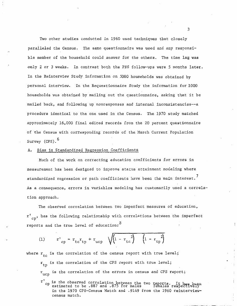
Two other studies conducted in 1960 used techniques that closely

paralleled the Census. The same questionnaire was used and any responsi-

ble member of the household could answer for the others. The time lag was

only 2 or 3 weeks. In contrast both the PES follow-ups were 5 months later.

In the Reinterview Study information on 5000 households was obtained by

personal interview. In the Requestionnaire Study the information for 1000

households was obtained by mailing out the questionnaire, asking that it be

mailed back, and following up nonresponses and internal inconsistencies--a

procedure identical to the one used in the Census. The 1970 study matched

approximately 16,000 final edited records from the 20 percent questionnaire

of the Census with corresponding records of the March Current Population

Survey (CPS).6

A. Bias in Standardized Regression Coefficients

Much of the work on correcting education coefficients for errors in

measurement has been designed to improve status attainment modeling where

standardized regression or path· coefficients have been the main interest.7

As a consequence, errors in variables modeling has customarily used a correla-

tion approach.

The observed correlation between two imperfect measures of education,

r' , has the following relationship with correlations between the imperfectcp

reports and the true level of education: 8

(1) r'cp

where r is the correlation of the census report with true level;tc

r tp is the correlation of the CPS report with true level;

r is the correlation of the errors in census and CPS report;ucp

r' cp is the observed c:orrela.ti.on between the two l:,eports Ith....l:i b·"'tlestimated to be .887 and .875 for males . te~a~es'respect1ve1y

in the 1970 CPS-Census Match and .9149 from the 1960 reinterview­census match.

4

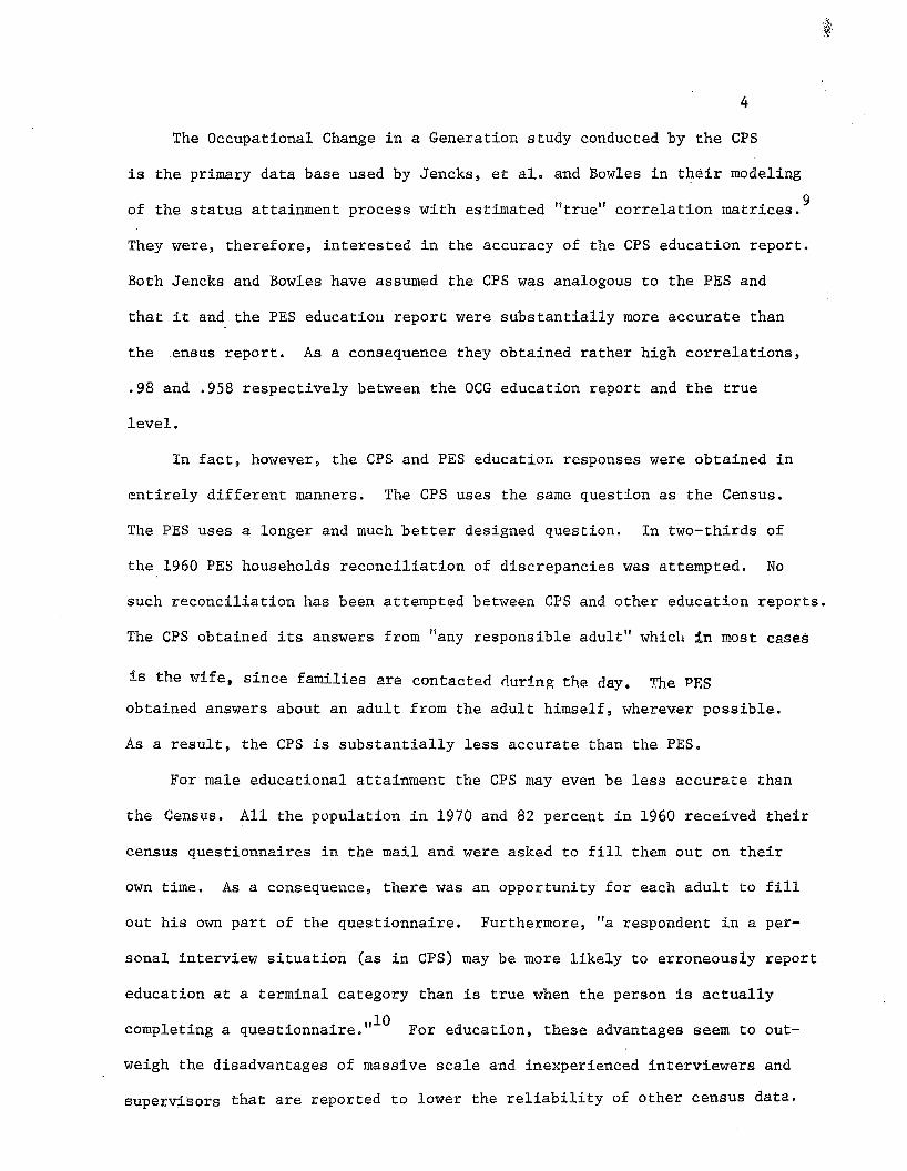
The Occupational Change in a Generation study conducted by the CPS

is the primary data base used by Jencks, et al. and Bowles in their modeling

of the status attainment process with estimated "true" correlation matrices. 9

They were, therefore, interested in the accuracy of the CPS education report.

Both Jencks and Bowles have assumed the CPS was analogous to the PES and

that it and the PES education report were substantially more accurate than

the .ensus report. As a consequence they obtained rather high correlations,

.98 and .958 respectively between the OCG education report and the true

level.

In fact, however, the CPS and PES educatioli responses were obtained in

entirely different manners. The CPS uses the same question as the Census.

The PES uses a longer and much better designed question. In two-thirds of

the 1960 PES households reconciliation of discrepancies was attempted. No

such reconciliation has been attempted between CPS and other education reports.

The CPS obtained its answers from "any responsible adult" which in most cases

is the wife, since families are contacted during the day. The PES

obtained answers about an adult from the adult himself, wherev.er possible.

As a result, the CPS is substantially less accurate than the PES.

For male educational attainment the CPS may even be less accurate than

the Census. All the population in 1970 and 82 percent in 1960 received their

census questionnaires in the mail and were asked to fill them out on their

own time. As a consequence, there was an opportunity for each adult to fill

out his own part of the questionnaire. Furthermore, "a respondent in a per-

sonal interview situation (as in CPS) may be more likely to erroneously report

education at a terminal category than is true when the person is actually

1 t · .. ,,10comp e 1ng a quest10nna1re. For education, these advantages seem to out-

weigh the disadvantages of massive scale and inexperienced interviewers and

supervisors that are reported to lower the reliability of other census data.

This heaping suggests

5

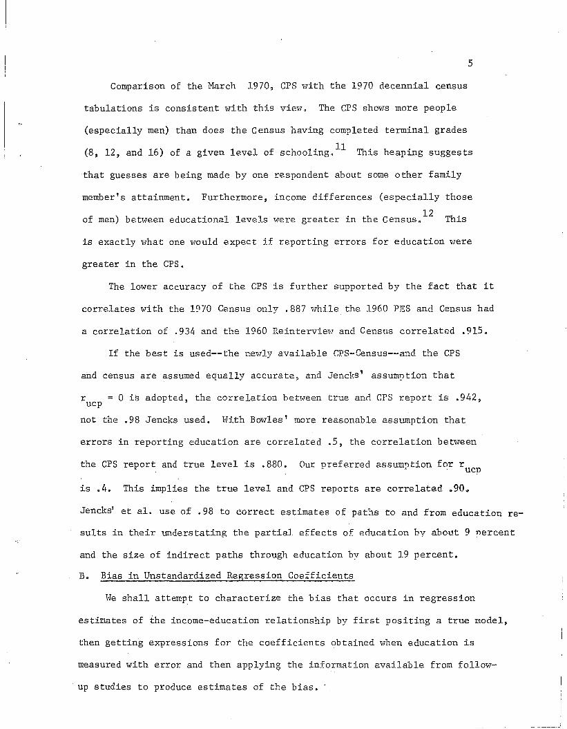
Comparison of the March 1970, CPS with the 1970 decennial census

tabulations is consistent with this view. The CPS shows more people

(especially men) than does the Census having completed terminal grades

(8 12 d 16) f . 1 1 f hI' 11, ,an 0 a g~ven eve 0 sc .00 ~ng.

that guesses are being made by one respondent about some other family

member's attainment. Furthermore, income differences (especially those

of men) between educational levels were greater in the Census.12

This

is exactly what one v70uld expect if reporting errors for education v7ere

greater in the CPS.

The lower accuracy of the CPS is further supported by the fact that it

correlates with the 1970 Census only .887 while the 1960 PES and Census had

a correlation of .934 and the 1960 Reintervi~v and Census correlated .915.

If the best is used--the newly available CPS-Census--and the CPS

and census are assumed equally accurate, and Jencks' assumption that

r = 0 is adopted, the correlation between true and CPS report is .942,ucp

not the .98 Jencks used. With Bowles' more reasonable assumption that

errors in reporting education are correlated .5, the correlation between

the CPS report and true level is .880. Our preferred assumption for r ucp

is .4. This implies the true level and CPS reports are correlated o90~

Jencks' et al. use of .98 to correct estimates of paths to and from education re-

suIts in their understating the partial effects of education by about 9 percent

and the size of indirect paths through education by about 19 percent.

B. Bias in Unstandardized Regression Coefficients

He shall attemp_t to characterize the bias that occurs in regression

estimates of the income-education relationship by first positing a true model,

then getting expressions for the coefficients obtained \vhen education is

measured with error and then applyin~ the information available from follow-

. up studies to produce estimates of the bias •.

6

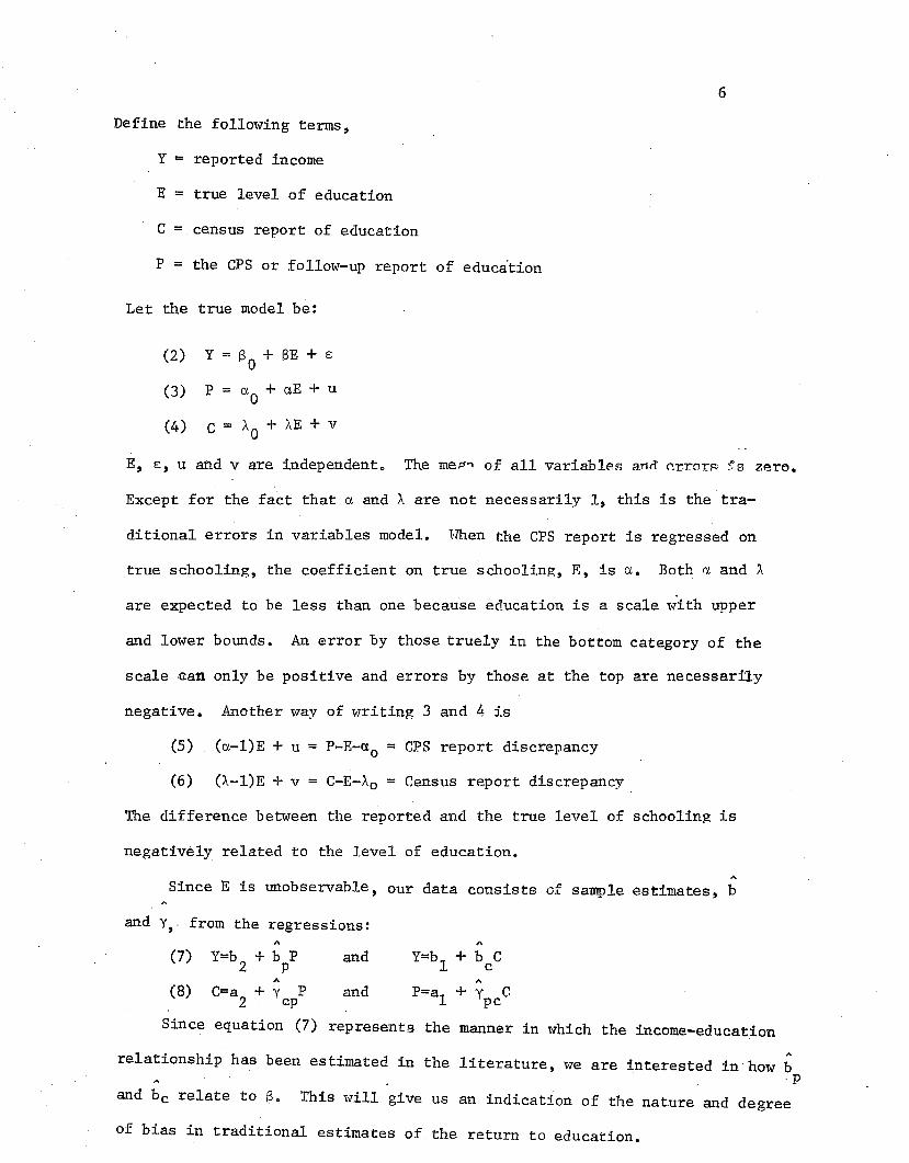
Define the following terms,

Y reported income

E = true level of education

C = census report of education

P = the CPS or follow-up report of education

Let the true model be:

(2)

(3)

(4)

Y ==S + SE + 80

P = aO

+ aE + u

C = 11.0

+ AE + v

E, 8, U and v are independentc The mep., of all variablp.fl an.(l 0.r.rDr~ ~s zp.ro.

Except for the fact that a and A are not necessarily 1, this is the tra-

ditional errors in variables model. vfuen the CPS report is regressed on

true schooling, the coefficient on true schooling, E, is a. Both ~ and A

are expected to be less than one because education is a scale with upper

and lower bounds. An error by those truely in the bottom category of the

scale ~an only be positive and errors by those at the top are necessarily

negative. Another way of writing 3 and 4 is

(5) (a-l)E + u = P-E-ao = CPS report discrepancy

(6) (A-l)E + v = C-E-Ao = Census report discrepancy

The difference between the reported and the true level of schooling is

negatively related to the level of education.

Since E is unobservable, our data consists of sample estimates, b

and Y,· from the regressions:

"(7) Y=b + b P2 p

"(8) C=a + Y P2 cp

Since equation (7)

"

"and P=al + y Cpc

represents the manner in which the income-education

relationship has been estimated in the literature, we are interested in how bp

and bc relate to S. This will give us an indication of the nature and degree

of bias in traditibnal estimates of the return to education.

7

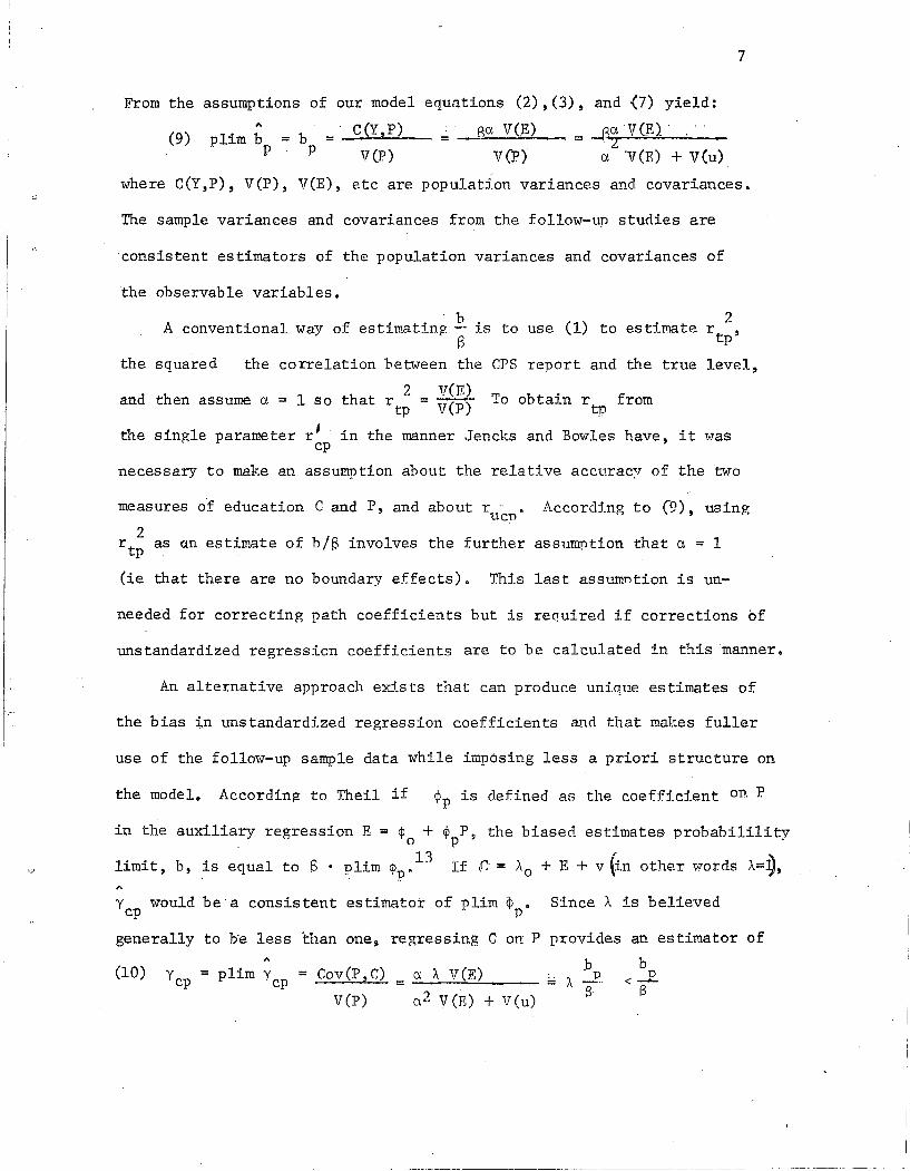
From the assumptions of our model

=

equations (2),(3), and (7) yield:

Pia VeE) p,aVQO'. = -:z

V(p) a 'V(E) + V(u)

C(Y,P)plim b = b = --=-~-~-~.. p p V(P)

(9)

,"where C(Y,P), V(P), VeE), etc are population variances and covariances.

The sample variances and covariances from the follow-up studies are

consistent estimators of the population variances and covariances of

the observable variables.

A conventional way of . . b. OJ estimate2

est~matlni!. -- ~s to use to rS tp'

the squared the correlation between the CPS report and the true level,

2 VeE)and then assume a = I so that r tp = V(p) To obtain r fromtp

the single parameter r l in the manner Jencks and Bowles have, it wascp

necessary to make an assumption about the relative accuracy of the two

measures of education C and P, and about r ucn According to (9), using

2r tp as an estimate of b/S involves the further assumption that a = I

(ie that there are no boundary effects). This last assumntion is un-

needed for correcting path coefficients but is required if corrections of

unstandardized regression coefficients are to be calculated in this manner.

An alternative approach exists that can produce unique estimates of

the bias in unstandardized regression coefficients and that makes fuller

use of the follow-up sample data while imposing less a priori structure on

the model. According to Theil if ¢p is defined as the coefficient on P

in the auxiliary regression E ... ¢ + ¢ P, the biased estimates probabilility- a p

limit, b, is equal to 6 . plim ¢u. 13 If r· = AO + E + v~n other words A=~,

y would bea consistent estimator of plim ~p. Since A is believedcp

generally to b'e less than one, regressing C orr P provides an estimator of

(10) .by cp = plim ycp = Cov(P, C) = .;;.;a---:.A_l.:...l.>.:(E~,) i= A -P,

V(p) a 2 VeE) + V(u) B·

b<-2.

(3

8

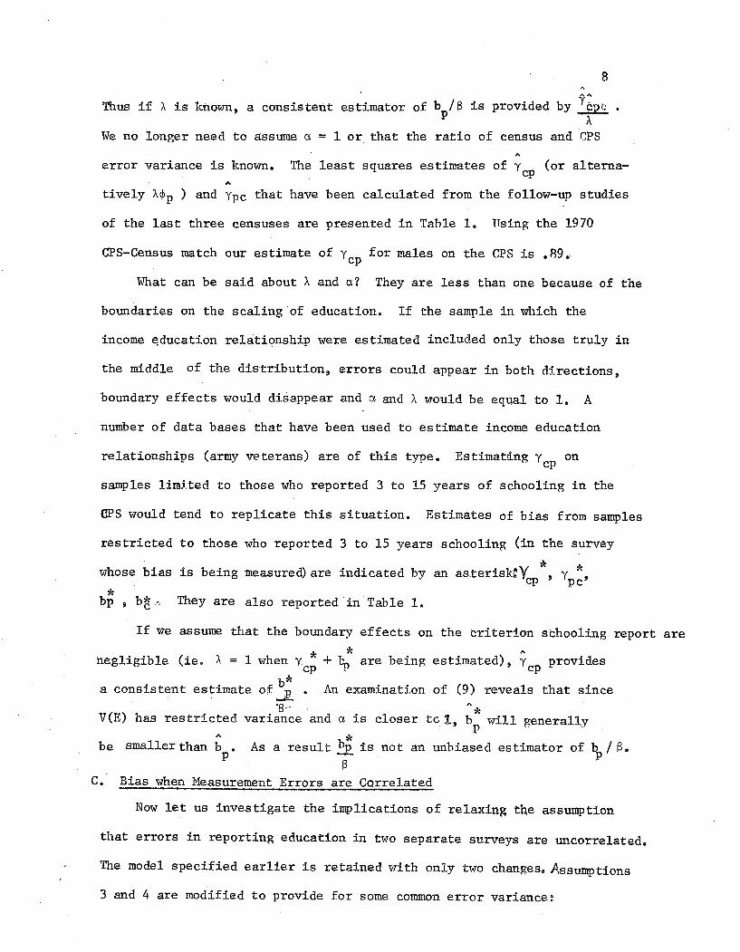
Thus if A is knovnl~ a consistent estimator of bp/S is provided by YPE <; •

;\

We no longer need to assume a = 1 or that the ratio of census and CPS

error variance is known. "The least squares estimates of y (or alterna­cp"tively A~p ) and Ypc that have been calculated from the follow-up studies

of the last three censuses are presented in Table 1. Usin~ the 1970

CPS-Census match our estimate of Ycp for males on the CPS is .B9~

What can be said about A and a? They are less than one because of the

boundaries on the scaling of education. If the sample in which the

income ~ducation relationship were estimated included only those truly in

the middle of the distribution, errors could appear in both directions ~

boundary effects would disappear and a and A would be equal to 1. A

number of data bases that have been used to estimate income education

relationships (army veterans) are of this type. Estimat~ng Y oncp

samples limHed to those who reported 3 to 15 years of schooling in the

CPS would tend to replicate this situation. Estimates of bias from samples

restricted to those who reported 3 to 15 years schoolin~ (in the survey

* *whose bias is being measured) are indicated by an asteriskn~p , Ypc~

*bp ,b~.. They are also reported in Table 1.

are being estimated)~ Y providescp

effects on the criterion schooling report areboundary

*+~

If we assume that the

*negligible (ie. A = 1 when Yep

b*a consistent estimate of-ll. An examination of (9) reveals that sinceoS" . "*

VeE) has restricted variance and a is closer tel, bp

will generally

" *be smaller than b • As a result ~ is not an unbiased estimator of bp / S.p S

C. Bias when Measurement Errors are Correlated

Now let us investigate the implications of relaxinp, the assumption

that errors in reporting education in two separate surveys are uncorrelated.

The model specified earlier is retained with only two changes. Assumptions

3 and 4 are modified to provide for some common error variance:

9

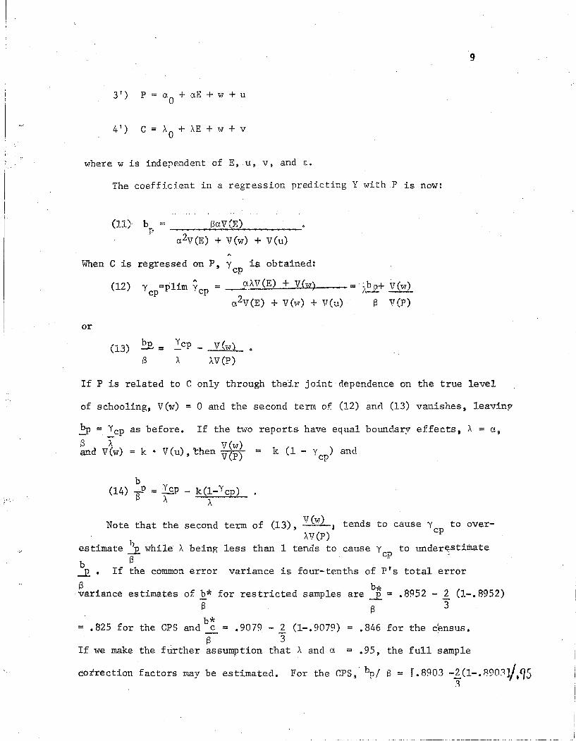
3 I ) P a 0 + aE + w + u

where w is independent of E, u, v, and E.

The coefficient in a regression predicting Y with P is now:

(11) (3aVon

o:2V(E) + V(v.l) + \leu)

When C is regressed on P, y is obtained:cp

(12) Ycp=p1im Ycp = ---2'.AV(E) + V(w)

a 2V(E) + V(w) + V(u)

= :,b p+ V(~q)1- __

S V(P)

or

(13) ~= ~cp - V(v.l).

S A W(P)

If P is related to C only through their joint dependence on the true level

of schooling, V(w) = 0 and the second term of (12) ann (13) vanishes, 1eavinp

.!Y = ~cp as before. If the two reports have equal boundary effec ts, A = a,

S. A V(w)and V(w) = k • V(u), then V(p) = k (1 - Ycp) and

b(14) ~p = Ycp - k(l-Ycp)

S A ';;";;":';:;;'A-"':~-

b)'(estimates of b* for restricted samples are -R = .8952 - 2 (1-.8952)

S S 3

variance is four-tenths of P's total error

to over-tends to cause Ycp

cause y to 1.lnder~stiIila.tecp-

error

Note that the second term of (13), V(w) )AV(P)

being less than 1 tends toes timate ~ while A

b S-E' If the commonSvariance

b*= .825 for the CPS and c = .9079 - ~ (1-.9079) .846 for the census.

S 3If we make the further assumption that A and a = .95, the full sample

cotrection factors may be estimated. For the CPS,' bpj S = [.8903 -2(1-.890~J/.~5.1

10

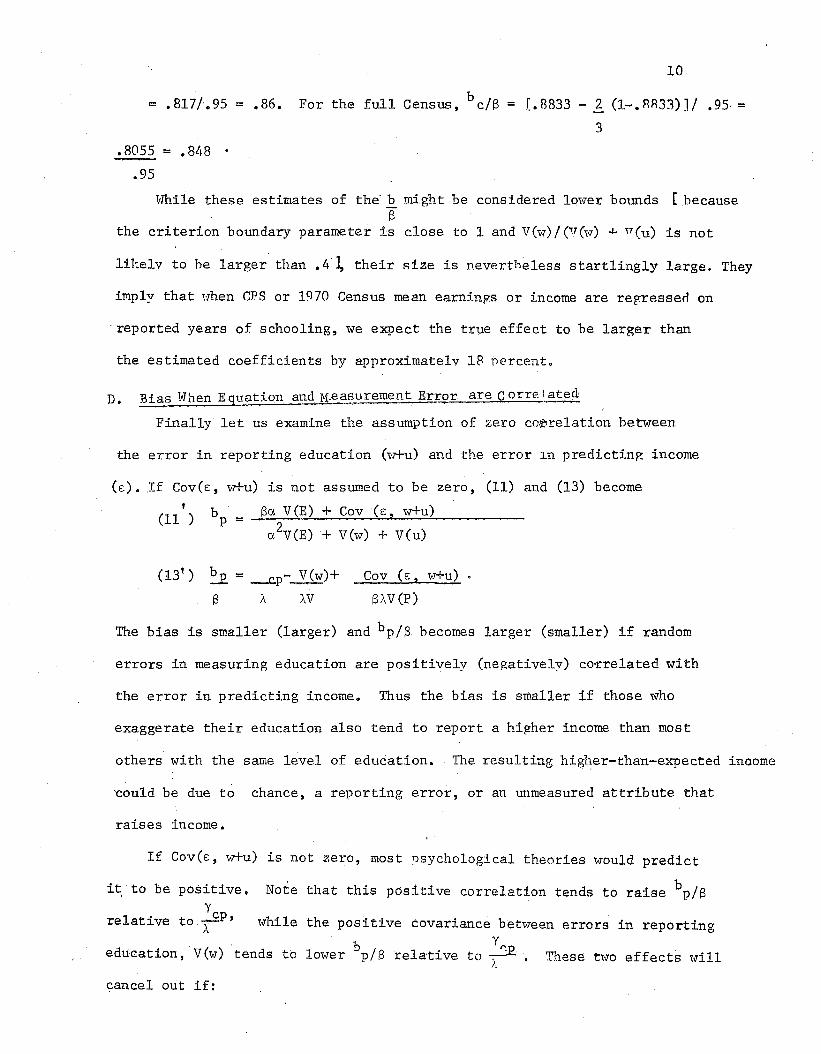
= .817t. 95 = .86. For the full Census, b ciS = r.. R833 - £ (1-. RR33)] I .95, =3

.8055 = .8l f8 •

•95

'VJhi1e these estimates of the' b might be considered lower bounds [becausee

the criterion boundary parameter is close to 1 and Vew) I ("('(,1) -l- IT(u) is not

lil~e1y to he larger than .4'], their size is nevertheless startlingly large. They

iNp1y that '(~hen CPS or 1970 Census mean earnin?s or income are regressen on

'reported years of schooling, we expect the true effect to be larger than

the estimated coefficients by approximatelv 18 percent.

D. Bias tA1hen Equation and M_easurement Error are Corre:,atett

Finally let us examine the assumption of zero car-relation be~7een

the error in reporting education (vr+u) and the error In predicting income

(E:) •.If Cov(E:, vr+u) is not assumed to be zero, (11) and (13) become

(11') bp = Sa VeE) + Cov(E:, w+u)

a2

V(E) + \lew) + V(u)

(13') ~ = ----e.p- V(w)+

13 A AV

Cov (E:. V7+U) .

SAV(P)

The bias is smaller (larger) and bp/S becomes larger (smaller) if random

errors in measuring education are positively (negatively) cOTre1atedwith

the error in predicting income. Thus the bias is smaller if those who

exaggerate their education also tend to report a higher income than most

others with the same level of education. The resulting higher-than-expected inoome

~ould be due to chance, a reporting error, or an unmeasured attribute that

raises income.

If Cov(E:, w+u) is not zero, most nsychological theories would predict

education, V(w) tends to

Note that this positive correlation tends to raise bp/S

These two effects will

it, to be

relative

positive.y

to ...,.£P,A '("hi1e the positive covariance between errors in reporting

b . ". y~lower piS relative to ~

cancel out if:

11

13 = COX(E, W+U) = 'COV(E, w)

V(W) V(W)

+' r.ov(e. U)

V (107)

Cov(f:.,~'i+JJ)1 V(W) ­

V(w+U) / v (W+U)

/,,)The interpretation of this condition is that the true income

education coefficient, 13, is equal to the coefficient of a regression of

E on the error in reporting education, divided by the coefficient pre-

Actually going to school for an

dicting one error in reporting educa tion ~·ri th another. If 13 is greater

than this ratio, bp/13 < ~cP.

extra year certainly raises income by more than systematically saying one went to

school for an extra year when one has not. Since w is the education

reporting error that occurs in both questionnaires, 13 > COy, (E, w)V(w)

Further, we can most likely safely assume that education reporting error

which does not recur in the second survey has a negligible correlation

models is to use individual

= .8833 = .930..95

estimating human capitalA common way of

COV(E,W) + COV(E,U)with E. Thus, if 13 > ., YCp/A places an unper bound

V(w)on bp / 13 • 'Retaining our earlier assumption that A = CJ, =.95', the upper

bound estimate of the CPS's bp/ 13 = .8903 = .937. T.he upper bound.95

for the Census bp j'(3

observations and the log of earnings as the dependent variable. Mincer

has observed that t~e coefficient on education in such regressions ~qhich

can be interpreted as a rate of return) is consistently lower than the

rates of return estimated direct1y.14 Predicting the log of earnings

with indiyidua1 data means one is assigning to each educational class

its geometric mean earnings. A 10 percent increase fram $1000 to $1100

affects the estimate to the same degree as a 10 percent increase from

$20,000 to $22,000. In positively skev7ed distributions, like income,

the regression line passes below each group' sarithmetic mean and dif-

ferences bebveen groups are understated. Since sk~roess increases

12

as education increases, estimates of the mean dollar difference between

groups are understated even more. Rates of return derived from this

specification are not comparahle to rates of return on other assets

and, without adjustment, should not be used for settinp: policy.

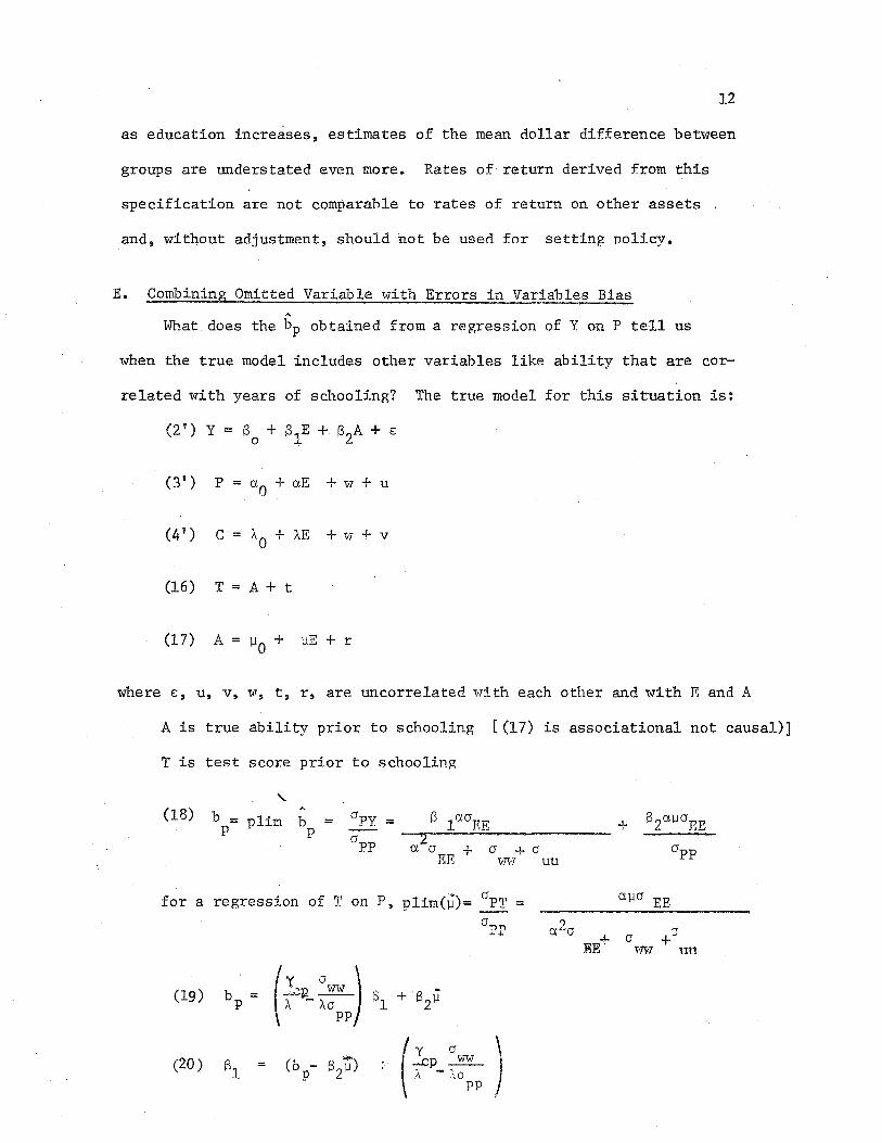
E. CombininB Omitted Variable with Errors in Varjm)les Bias

What does the bp obtained from a regression of Y on P tell us

when the true model includes other variables like ability that are cor-

related with years of schooling? The true model for this situation is:

(3') P = 0'.0 + aE + w + u

(4') C = AO + AE + W + v

(16) T = A + t

(17) A = ~O + ~E + r

where €, u, v, w, t, r, are uncorrelated with each other and with E and A

A is true ability prior to schooling [(17) is associational not causal)]

T is test score prior to schooling

(18)"-

b = plim b =p p apy = S 1aaEE +

a - ......2-=--:;..;.;;.:;...-------PP a. a + a + a

EE V~'I uu

for a regression of T on P, plim(~)= apT =: a~a EEa':")n ')

'-" a"'a-I- 0- +:J

:RE' 'F!VT un

(19) b = (_~p aww )13 + B2Gp A - AO 1pp

(20 ) S (b - S}7) (y "ww ).-..cp __I p A - \0

pp

13

or if the true ~ is known,

(21) Bl = b 1- Y a 13 211.p ~- ww- -A

;"app

Combining the two corrections is straightforward. The first require-

ment is an estimate of the true effect of ability on earnings, 132

, Next

using the population from which b was estimated, the amount by which those

with higher reported schooling have higher prior test scores is calculated.

The product of these parameters is subtracted from b and the adjustment

factor derived earlier in (13) is applied.lS

F. Bias in Rates of Return Calculated from Census Tabulations

Most human capital studies use published census tabulations that group

people into a fe~v classes by years of education attained. Grouping on the

independent variable generally reduces the size of the errors-in-variables problem. 16

If one is interested in an estimate of the'true earnings gain from a

particular level of schooling, estimates of an errors-in-variables correction

derived from samples encompassing the full range of education may not be

appropriate. The process that generates reporting errors may not be regular

(i.e., characterizable simply by C - E = A + (A-l)E + u where the distribu­o

tion of u is independent of E). The availability of detailed cross tabula-

.tions of Census and follow-up education reports allows us to calculate

estimates of the bias ~ for ad]' acent education classes vrithout as'suming u isb -

independent of E.

Using tabulations of Census and follow-up enucation reports for

1960 and 1970, an estimate was made of the true earning increments behieen

adjacent education classes. A true earnings level was assigned to each year

of educational attainment. This level was assumed to be the mean for the

corresponding criterion education report. A weighted average of these means

for each census reported education class corresponds to the earnings averages

14

17that census tabulations produce. This procedure drops the assumption

that the process that generates errors in the census report is regular and thereby

allows for heaping effects. The results presented in Table 2 assume

(1) the error in the criterion report is uncorrelated with the true level

of schooling (a = 1) and with the census reporting error (0 = 0) anduv

(2) the error in the Census report is uncorre1ated with earnings (0 = 0).f5l

The assumption of no boundary effects in the criterion report is

almost certainly violated for intervals adjacent to the boundary (0-7

versus 8 and 16 versus 17+). The b:tas crtimatcc (0:;:" those intevalc arc,

"1.t= ., ·18(..Llere.:..ore, t00 _.ar?;"-_

As expected the results in Table 2 imply that different schooling

increments have different biases. The large estimated biases for elementary

and postgraduate schooling exaggerate the true bias because of boundary

effects on the criterion schooling report. Census tabulations seem to

consistently overestimate the earnings gain from the first two years of high

school. For women in 1970 and everyone in 1960 the earnings gain of the

first two years of college are underestimated in the Census by almost 20

percent. The CPS seems to underestimate the male earnings increments for

8 through 16 years of schooling by more than the Census does. For females,

in contrast, C~nsus and the CPS bias estimates are quite similar.

The effect of adjusting the return to college graduation for ability differ"--

ences will be examined. The ratios of high school graduate to college

graduate rarnings were .747 for ages 25 to 34, .624 for ages 35 to 54, and

.599 for ages 55 to 64. Prior to college, college graduates typically had

IQ '8 one standard deviation above

15

those who did not enter college. If we adopt 7 percent as the true reduc-

tion in earnings that occurs if a college graduate has the same ability as

the typical high school graduate, the earnings increment for ages 25 to

34 is reduced by 28 percent and the earnings increment for 35 plus is

19reduced by approximately 18 percent. The errors in variables adjustment

is then multiplied by the proportion of the gross effect remaining [(i.e.,

for 25 to 34,S f b = 1.056 (1 - .747 - .07) f (1 - .747) = .76».

II. Coverage Bias: Errors in Measuring a Person's Contribution to Output

The second major source of bias in estimating social returns derives

not from random errors, but from systematic undercounting. Reported earn-

ings do not provide complete coverage of a worker's total compensation and

do not include taxes paid by employers on output or on labor input. The

bias from this source will be called coverage bias. The contribution to

total output of a marginal increment in a given factor of production is its

marginal physical product times the price consumers pay for the product.

A profit maximizing firm will arrange its use of factors so that the total

compensation paid including taxes for a marginal increment of a factor

equals that factor's marginal revenue product. Discrepancies arise between

reported earnings and total cost of labor input due to under or overr&?ort~ng

incomplete coverage, and employer paid taxes on employee wages. Discrepancies

may arise between marginal revenue and consumer price due to excise taxes or

monopoly power.

It is possible to determine the average degree of under or overr~portine

to Census interviewers for each type of income by comparing national income

aggregates derived from establishment sources with the aggregates implied

by the Census household data. Doing this for the March 1970 and March 1971

CPS we find that the unreported component of money earnings was 5.4 percent

1620

of the money earnings reported to Current Population Survey interviewers.

While 96 percent of wage and salary income was reported, only 52 percent of

farm income was reported. This will cause significant understatement of mean

incomes and income differentials of agricultural states. The 1970 Census

comes substantial~y closer to its control aggregates than the CPS for that

year. In Table 3 we reconcile CPS and Census aggregates to National Income

Account aggregates. The percent of aggregate earnings missed was only 1.5

percent in 1970 Census and seven-~enths of a percent in the 1960 Census.

Census and CPS aggregates may be low either because people are missed

or because on average each person understates his earnings. The Bureau of

the Census has developed estimates of the amount by which the nation's

21population was understated in the Census and the CPS. Applying age, sex,

and race specific undercount rates to 1970 Census estimates of their earnings

aggregates and assuming that those missed earn two-thirds the average, our

adjustment for the undercount increases Census aggregates by 2.1 percent in

1960, and 2.8 percent in 1970. This implies in turn that per capita earnings

on the Census overstated national accounts per capita earnings by 1.47 percent

in 1960 and 1.34 percent in 1970. The CPS understated national account per

capita earnings by 2.8 percent.

Another source of discrepancy between reported earnings and total

compensation received are food and housing received as pay, farm products

consumed at home, and employer contributions to private pension plans.

Estimates of the amount of each of these received by each income class

are available in Roger A. Herriot and Herman P. Miller's, "Who Paid the22

Taxes in 1968." The major element of these imputations, employer contri-

butions to pension plans, was assumed to be proportional to wages and salaries.

Together these imputations average 5 percent of reported income. Employer

17

contributions to private pension and welfare funds has been a rising propor-

tion of total employee compensation in the last few decades. As a result

the imputation adjustment for 1959 is 1.3 percentage points less than the

one described in Table 3 for 1968 and 1969.

The final discrepancy between reported earnings and the marginal revenue

product are the Social Security and Unemployment Insurance taxes paid by

employers. These taxes declined as a proportion of earnings because in 1969

the social security tax was paid only on the first $7800 of Nages and the

unemployment insurance taxes were paid only on the first ·$3400 of wages.

The statutory rate (4.8 percent for social security and 1.4 percent for

unemployment insurance) was used for earnings brackets below the maximum23

taxable wage. Above that the average social security tax rate was the

maximum tax, $374, divided by the midpoint of the earnings interval and

the average unemployment insurance tax rate was $47.60 divided by the mid-

point. Since 1969 the Social Security tax rate has risen from 4.8 to 5.85

percent and the maximum taxable wage has risen from $7800 to $10,800. The

1969 rates are used because the adjustments are intended for use with

decennial census data. If the earnings data being used are for a period of

higher tax rates, and employers have had time to adjust, a larger adjust-

ment for labor input taxation would be in order. In 1959 Social Security

tax rates were 2.5 percent on the first $4800. Therefore, calculations24

of coverage bias for 1959 use the lower tax rate applicable then.

Th~ final adjustment must take us from marginal revenue product to

the consumer's valuation of that output. Both monopoly power and taxes

cause consumer price to exceed marginal revenue. State and federal sales

and excise taxes, not including alcohol and tobacco taxes, totaled $27.6

billion in 1968 or approximately 3.2 percent of GNP. Alcohol and tobacco

18

taxes are excluded because they are assumed to reflect the negative exter-

nalities a person's use of these products imposes on others. The dollars

of excise revenue generated by a person's work were calculated by multiply-

ing the sum

earnings by

of labor input taxes

1 ~.033, (.968 - 1).

and reported, unreported, and imputed

Whether monopoly power makes a further correction desirable depends

upon the source of the monopoly and which factor of production is receiving

the monopoly rents. If monopoly rents add equal percentage increments

to workers' wages and to capital's return, no problem is created, for our

comp~nsation data has already captured them. If a firm faces close to

infinitely elastic long-run demand curve at its limit price, but neverthe-

less receives monopoly rents because of the ownership of some unique factor

of production (e.g., patents, control of best raw material sources,

government licenses), no adjustment is required. An add on is required

only where P > LRMR = LRMC and where the monopoly rents do not get paid

to labor.

How large might such monopoly profits be? Harberger's upper bound

estimate of the welfare impact of monopoly implied that one-third

of manufacturing prof~~s were excess' profits. 26

Assuming that the share of monopoly rents [(P - LRMC)q] in corporate

profits is one-third for manufacturing and one-tenth for nonmanufacturing,

we obtain an upper bound estimate of $17.7 billion for 1969 or 1.9 percent

27of GNP. . The results presented in Table 3-5 do not include an adjustment

28for monopoly distortions or for systematic economies of scale.' The reader

may make his own adjustment for monopoly with his own assumption about monopoly

by simply multiplying the average and marginal ratios of social benefit to

reported income in Table 4-6 by a number between land 1.019.

19

Putting all these adjustments together we find that the average social

productivity benefit of a person's work--the sum of after tax earnings and

taxes generated--averages about 120 percent of reported earnings. As earnings

rise, the ratio of social benefit to reported earnings tends to fall from

1,20 to 1.13. The fall in the ratio is a consequence of imputations not

rising as fast as income and the zero marginal social security tax on wages

above $7800.

What portion of this total or social return can the individual be

expected to take into account when he makes his own decisions? Splitting

the social return into private and public components is necessarily more

arbitrary than calculating the total return. Table 4 presents lower bound

estimates of the private share of the total return. It is based upon the

assumption that extra earnings do not, on the margin, place any additional

burden on the government's provision of services. This is a valid assump-

tion for pure public goods--defense, foreign affairs, space, and police and

fire protection. Providing an individual with more of a pure public gOOtl

inevitably means everyone else gets more.

However, for many government services provided at zero or nominal

cost, providing the service to one person means it must be denied to some-

one else. If usage of such services rises with income, extra after tax

income places an additional burden on other taxpayers. Directly provided

services of this kind are education, libraries, airports, congested high­

29ways, recreation, sewers, water supply, and garbage collection. Dsage

of certain other services--:lbod 9:amps , directly subsidized housing, Medicaid,

unemployment insurance and AFDC--go do,vn as earnings rise. If one takes a

life cycle perspective, however, the largest of transfer programs, social

security, provides larger dollar 'benefits to people with higher earnings.

20

The net impact of earnings on usage of government programs is likely to be30

positive, though it may be small (i.e., 3 or 4 percent). In exceptional

cases, an education or health intervention that increases after tax earnings

may actually decrease total gov~rnment expenditures. For Black females, the

present value of expected welfare payments is about $7 000 less fCt high

school graduates than for dropouts. This reduction is likely to be larger

than the increase in services that are positively associated with education

and earnings.

By neglecting these impacts of government programs, the private bene-

fit of labor market productivity can be estimated simply by subtracting

personal income taxes and the employee's share of Social Security taxes

from the sum of reported earnings, unreported earnings, and imputations.

In almost all cases, this places a lower bound on the estimate of the

private return. The average incidence of federal and. state income tax

payments were taken from Herriot and Miller's "Who Paid Taxes in 1968."

The incidence of Social Security taxes on earnings has already been

described. The sum of these two taxes rises from 8.9 percent of reported

earnings in the $2000-$4000 bracket to 17.4 percent in the $15,000-$25,000

bracket. The ratio of disposable earnings (private returns) to reported

earnings, therefore, falls from 1.01 to .905 as one moves from low to high

brackets. The ratio of all taxes generated to reported earnings rises from

.19 to .23 as earnings rise.

Marginal ratios of after tax earnings to reported earnings and of taxes

generated to reported earnings were estimated by the fol~owing procedure.

Average ratios were calculated separately for·each bracket. After tax income

and total tax generated were calculated for the representative family in the

interval using average ratios and the midpoints of the intervals as family

21

rates of taxes generated as reported income increases were above their

averages and were generally declining with income. They decline because

the drop in the marginal rate of Social security tax from 9.6 percent

to zero outweighs the progressivity of the personal income tax. The

marginal rates of private return after tax earnings, were below the

average and tended to fall with income from a high of .935 to .89. Largely

because of the declining ratio of Social Security taxes to earnings as earn­

ings increase, the marginal ratio of social or total return to reported

earnings is also below the average. It falls from 1.19 in low brackets to

1.12 in high brackets.

III. Implications of Coverage Bias

Most studies that have attempted to measure social and private returns

to education have neglected the effects of underreporting, fringe benefits,

and employer paid taxes on wages ~nd value added. To what extent does this

bias their results? Table 4 presents recommended adjustments for coverage

bias and progressive income taxation for each census and for the CPS.

Since most of the calculations of returns to education have been

presented as rates of return, no problem is created if the measures of

both cost and benefits are biased to the same degree. Measures of foregone

earnings are subject to the same type of coverage bias as benefit measures.

In fact, because foregone earning changes occur in the lower range, their

coverage bias is proportionally larger. Also the split between taxes gener­

ated and private costs is different. The young people who are investing

time in their own education face lower or zero rates 6f income taxation.

As a consequence private rates of return (especially those of the lowest

schooling levels) are lowered by adjustments for coverage bias and taxation.

22

Social costs include, however, a large government expense component

which does not suffer coverage bias. If for college graduation instruc­

tional costs are equal to foregone earnings, a CPS coverage bias adjust­

ment would make costs 8 percent higher and benefits 13 percent higher.

Thus, the true rate of return will be 1.05 times the conventionally

calculated return. This is not a very large bias especially when one

considers that estimates of returns on physical capital are affected

by one of the biases enumerated above (value added taxation).

Coverage bias is a serious problem when costs of a student's time

are actually leisure foregone or when the student's time commitment does

not change. This latter situation occurs when a government educational

intervention is being evaluated. If we are calculating the costs and

benefits of improving ~he quality of education, providing a specialized

service for problem children, or subsidizing some college instructional

programs more than others, current practice counts all the costs but only

some of the benefits. The ratios presented in the social productivity

~enefit section of Table 4 are the correction factor that should be applied

to the benefit cost ratios of increases in the quality of education. There­

fore, coverage bias produces a systematic downward bias of 8 to 18 percent

in the calculated social benefit-cost ratio depending on which level of

education the intervention is at.

If the time spent by the student on school work actually comes at the

expense of l'eisure rather than employment the social cost of that time is

less. Most young people have control over the number of hours they work for

wages. They, therefore, adjust th~ir work time until on the margin an hour

of leisure is worth to them approximately what they get from one more hour of

23

employment> the after tax wage rate. When a student's' time comes at the

expense of involuntary unemployment rather than voluntary leisure, the

social cost is even less.

The extra leisure time a nonstudent has does not produce taxes,

however, so the social cost of his lost leisure is equal to the private

cost. Thus when time spent in school is at the expense of leisure yet

that time has been valued at the money wage, the understatement of the

social rate of return is the greatest.

Errors in reporting educational attainment produces an identical. bias

in private and social rates of return to extra years of schooling. They

affect different educational increments differently, however. The under-

statement of rates-of-return and of benefit-cost ratios is largest for

grade school and the first few years of college. The returns to starting

high school are not understated and may in fact be overstated.

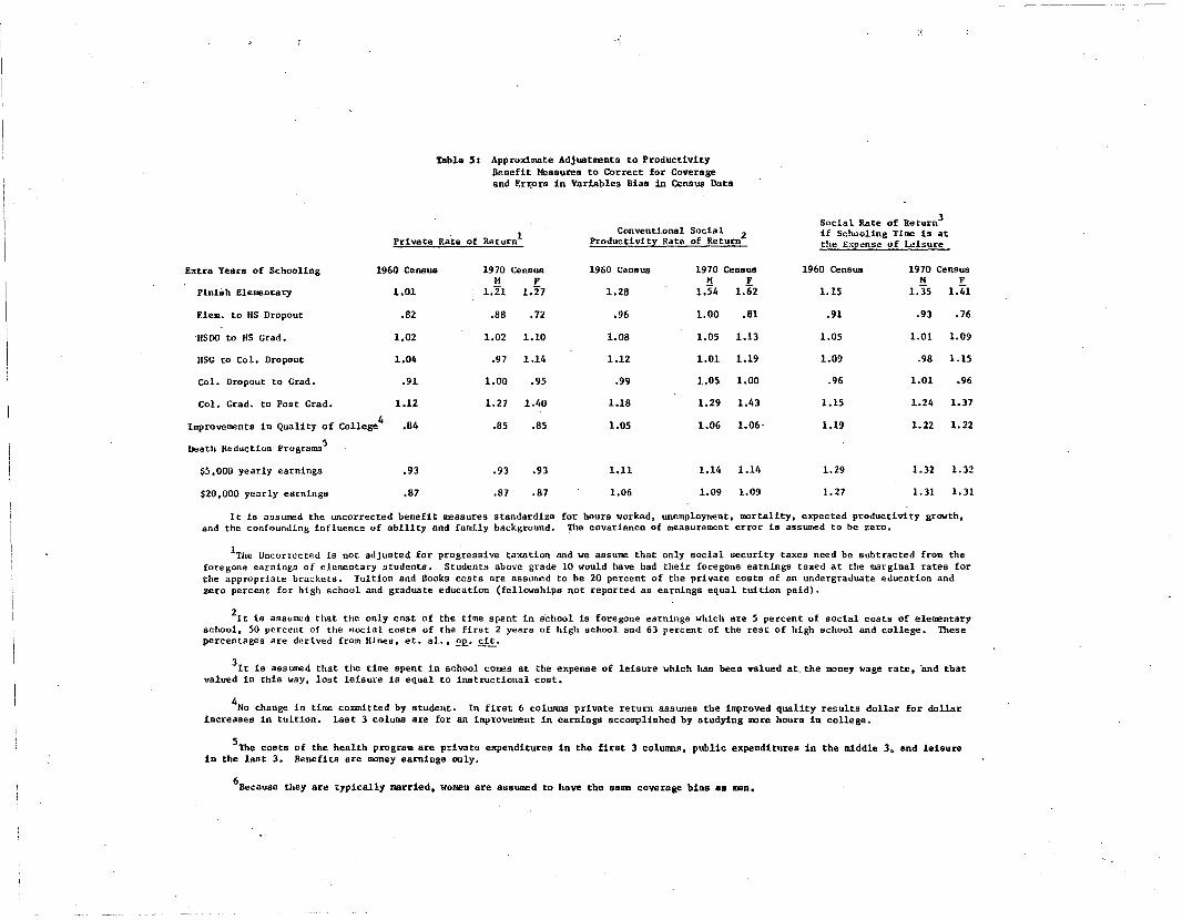
Table 5 presents the estimated ratio of corrected to uncorrected benefit

measures for different increments in education and for different data sources.

In most cases, whether or not an educational project is undertaken will not

depend on a bias of this size. However, given the simplicity of the adjust-

ment required, there is no reason not to use the correct productivity benefit

concept. It is interesting to note that the understatement bias is greater

for investments in low wage workers. Thus, benefit-cost ratios for euuca-

tional investments in discriminated minorities, women, secondary education

and low-skill workers are understated more than investments in college or

graduate education. The benefits of healt~~i~ents are understated more(/-

as well because here average ratios of true productivity to reported ear~~,

ings are relevant.

\

."

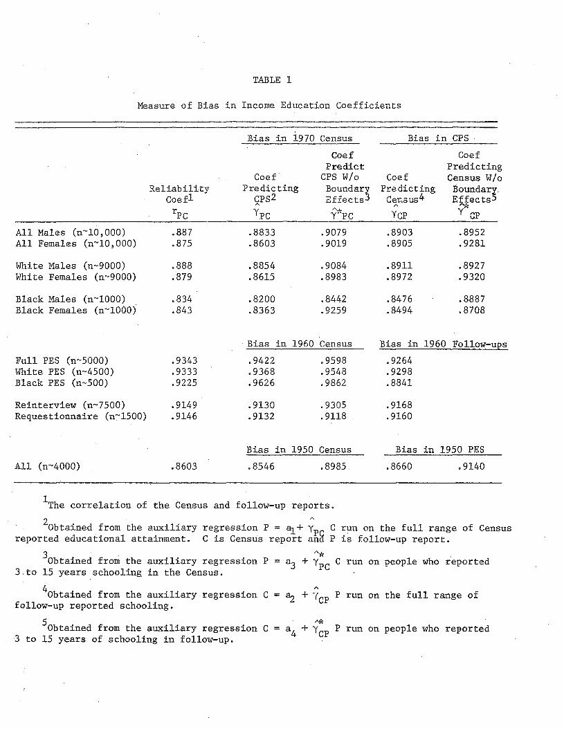
TABLE 1

Measure of Bias in Income Education Coefficients

Bias in 1970 Census Bias in CPS

Coef CoefPredict Predicting

Coef CPS wlo Coef Census wloReliability Predicting Boundary Predicting Boundarl

Coefl CPS2 Effects3 Cer..sus 4 EffectsA A A.~

rpC YpCA~"

Yep Y CPy"PC

All Males (n~lO,OOO) .887 .8833 .9079 .8903 .8952All Females (n~lO,OOO) .875 .8603 .9019 .8905 .9281

White Males (n~9000) .888 .8854 .9084 .8911 .8927White Females (n~9000) .879 .8615 .8983 .8972 .9320

Black Males (n~lOOO) .834 .8200 .8442 .8476 .8887Black Females (n~lOOO) .843 .8363 .9259 .8494 .8708

. Bias in 1960 Census Bias in 1960 Follow-ups

Full PES (n~5000) .9343 .9422 .9598 .9264White PES (n~4500) .9333 .9368 .9548 .9298Black PES (n~500) .9225 .9626 .9862 .8841

Reinterview (n~7500) .9149 .9130 .9305 .9168Requestionnaire (n~1500) .9146 .9132 .9118 .9160

Bias in 1950 Census Bias in 1950 PES

All (n~4000) .8603 .8546 .8985 .8660 .9140

1The correlation of the Census and follow-up reports.

20btained from the auxiliary regression P = al+;p C run on the full range of Censusreported educational attainment. C is Census report an~ P is follow-up report.

A*= a3 + YpC C run on people who reported30btained from the auxiliary regression P

3.to 15 years schooling in the Census.

40btained from the auxiliary regression C =follow-up reported schooling.

50btained from the auxiliary regression C =3 to 15 years of schooling in follow-up.

A

Bz + "(cp P run on the full range of

A*a4 + YCP P run on people who reported

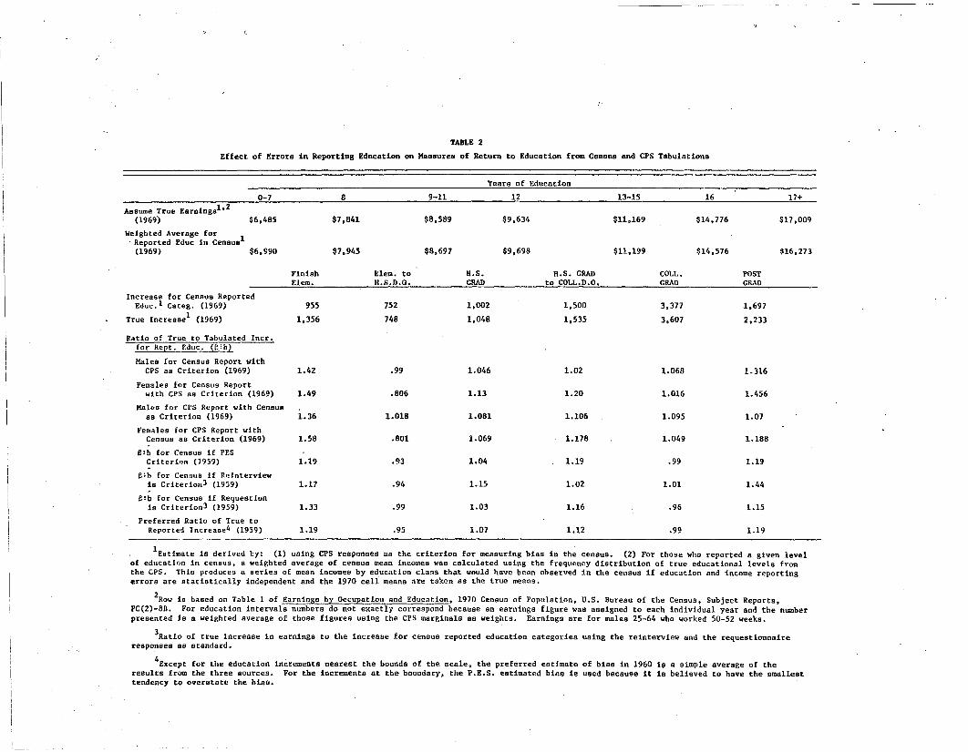
TABLE 2

Effect of Errors in Reporting Education on Measures of Return to Education from Census snd CPS Tsbulations

Years of Education

0-7 8 9-11 12 13-15 16 17+

Assume True Earningsl ,2(1969) $6,485 $7,841 $8,589 $9,634 $11,169 $14,776 $17 ,009

Weighted Aversge for. Reported Educ in Census1

(1969) $6,990 $7,945 $8,697 $9,698 $11,199 $14,576 $16,273

Finish Elem. to H.S. H.S. GRAD COLL. POSTElem. H.5.D.0. GRAD to COLL.D.O. GRAD GRAD

Increase for Census ReportedEduc. 1 Csteg. (1969) 955 752 1,002 1,500 3,377 ·h697

True lncreasel (1969) 1,356 748 1,048 1,535 3,607 2,l33

!latio of True to Tabulated lncr.for Rept. Educ. (e:b)

Hales for Census Report withCPS as Criterion (1969) 1.42 .99 1.046 1.02 1.068 1.316

Females for CenSU9 Reportwith CPS aa Criterion (1969) 1.49 .806 1.13 1.20 1.016 1.456

Hales for CPS Report with Censusas Criterion (1969) 1.36 1.018 1.081 1.106 1.095 1.07

Females for CPS Report withCenSUB as Criterion (1969) 1.58 .801 1.069 1.178 1.049 1.188

elb for Census if PESCriterion (1959) 1.19 .93 1.04 1.19 .99 1.19

e; b for Census if Rn Interviewis Criterion3 (1959) 1.17 .94 1.15 1.02 1.01 1.44

elb for Cen9ua if Requestionis Criterion3 (1959) 1.33 .99 1.03 1.16 .96 1.15

Preferred Ratio of True toReported Increaae4 (1959) 1.19 .95 L07 1.12 .99 1.19

lEatimate is derived by: (1) using CPS responses as the criterion for measuring bias in the census. (2) For those who reported a given levelof educstlon in census, a weighted average of census mean incomes was calculated using the frequency distribution of true educational levels fromthe CPS. This produces a aeries of mean incomes by education class that would have been observed in the censua if education and income reportingerrora are statistically independent and the 1970 cell meana are taken as the true means.

2Raw ia baaed on Table 1 of Earnings by Occupation snd Education, 1970 Censua of Population, U.S. Bureau of the Census, Subject Reports,PC(2)-8B. Por education intervals numbers do not exactly correspond because an earnings figure was assigned to each individual year and the numberpresented is a weighted average of those figures using the CPS marginsls 8S weights. Earnings are for males 25-64 who worked 50-52 weeks.

3Ratio of true increase in earnings to the increase for census reported education categories using the reinterview and the requestionnaireresponses as standard.

4except for the education increments nearest the bounds of the Bcale, the preferred estimate of biaB in 1960 is a simple average of theresults from the three sources. For the increments at the boundary, the P.E.S. estimated biaB is used becsuse it is believed to have the smallesttendency to overstate the biaB.

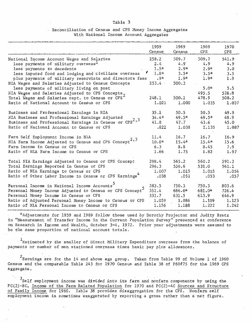
Table 3

Reconciliation of Census and CPS Money Income AggregatesWith National Income Account Aggregates

National Income Account Wages and Salariesless payments of military overseas lless payments to decedentsless imputed food and lodging and civilians overseas 'plus payments of military reservists and directors fees

NIA Wages and Salaries Adjusted to Census Conceptsless payments of military living on post

NIA Wages ahd Salaries Adjusted to CPS Concepts 2Total Wages and Salaries rept. to Census or CPSRatio of National Account'to Census or CPS

Business and Professional Earnings in NIANIA Business and Professional Earnings AdjustedBusiness ,and Professional Earnings in Census or CPS 2 ,3Ratio of National Account to Census or CPS

1959Census

258.22.41.5*1.8*

o 9"J'c

253.4

248.11.021

35.134.4''(41.8

.822

1969Census

509.74.92.9*3.5*1. 9*

500.3

500.11.000

50.549.5*47.71.038

1969CPS

509.74.92.9*3.5*1.9*

5.0*495.5478.9

1.035

50.549.5*43.61.135

1970CPS

541.94.93.03.51.9

5.5526.8508.2

1.037

49.948.945.01.087

2 3and CPS Concept 'Farm Self Employment Income in NIANIA Farm Income Adjusted to CensusFarm Income in Census or CPSRatio of NIA Farm Income to Census or CPS

11.410.6*

6.31.66

16.715.4*8.81. 75

16.715.4*8.451.82

16.915.6

7.91. 97

Total NIA Earnings Adjusted to Census or CPS ConceptTotal Earnings Reported in Census or CPSRatio of NIA Earnings to Census or CPSRatio of Other Labor Income to Census or CPS Earnings 4

Personal Income in National Income Accounts5 5Personal Money Income Adjusted to Census or CPS ConceptPersonal Money Income in Census or CPSRatio of Adjusted Personal Money Income to Census or CPSRatio of NIA Personal Income to Census or CPS

298.4296.3

1.007.038

383.5351.4331. 7

1.0591.156

565.2556.6

1.015.051

750.3686.0*631.5

1.0861.188

560.2531.0

1. 055.053

750.3681.0*613.9

1.1091.222

591.3561.1

1. 054.057

803.6726.4646.9

1.1231.242

*Adjustments for 1959 and 1969 follow those used by Dorothy Projector and Judity Bretzin "Measurement of Transfer Income in the Current Population Survey" presented at conferenceon Research in Income and Wealth, October 3-4, 1972. Prior year adjustments were assumed tobe the sgme proportion of national account totals.

lEstimated by the smaller of Direct Military Expenditure overseas from the balance ofpayments or number of men stationed overseas times basic pay plus allowances.

2Earnings are for the 14 and above age group. Tgken from Table 99 of Volume 1 of 1960Census and the comparable Table 243 for 1970 Census and Table 38 of P601f75 for the 1969 CPSaggregate.

3Self employment income was divided into its farm and nonfarm components by us;ing thePC(2)-8C, Income of the Farm Related Population for 1970 and PC(2)-4C Sources and Structureof Family Income for 1960. Table 38 provides disaggregation for the CPS. Nonfarm selfemployment income is sometimes 'exaggerated by reporting a gross rather than a net figure.

40ther labor income is primarily fringe benefits--employer contributions to privatepension plans and compe~sation for injuries.

SThe difference between personal income in the national accounts and adjusted personalmoney income is primarily imputations for owner occupied housing, services provided free byfinancial intermediaries, and payments to fiduciaries and decedents. 1960 estimates ofadjusted OBE personal income are from Herman Miller, Income Distribution in the United

0States, p. 173.

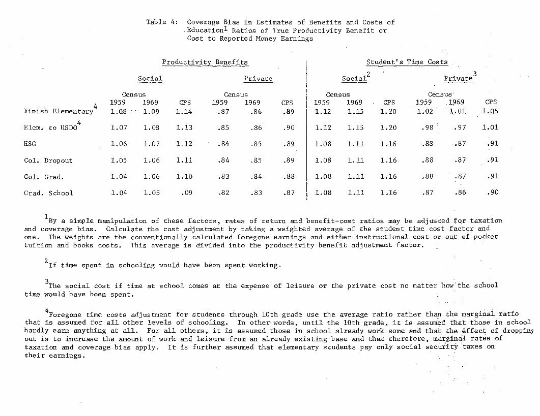
Table 4: Coverage Bias in Estimates of Benefits and Costs of-Educationl Ratios of True Productivity Benefit orCost to Reported Money Earnings

Productivity Benefits Student's Time Costs

Social Private Socia12 Private3

Census Census Census Census'

4 1959 1969 CPS 1959 1969 CPS 1959 1969 CPS 1959 ,:t969 CPSFinish Elementary L08 1.09 L14 .87 .86 .89 L12 LIS 1. 20 1.02 1.01 LQ5

Elem.4

1.13 I .98 .97 1.01to HSDO 1.07 1.08 .85 .86 .90 1.12 1.15 1.20

HSG 1.06 1.07 1.12 .84 .85 .89 1.08 1.11 1.16 .88 .87 .91

Col. Dropout 1.05 1.06 1.11 .84 .85 .89 1.08 1.11 1.16 .88 .87 .91

Col. Grad. 1.04 1.06 1.10 .83 .84 .88 1.08 1.11 1.16 .88 .87 .91

Grad. School 1.04 1.05 .09 .82 .83 .87 1.08 1.11 1.16 .87 .86 .90

lBy a simple manipulation of these factors, rates of return and benefit-cost ratios may be adjusted for taxationand coverage bias. Calculate the cost adjustment by taking a weighted average of the student time cost fa~tor andone. The weights are the conventionally calculated foregone earnings and either instructional cost or out of pockettuition and books costs. This average is divided into the productivity benefit adjustment factor.

2If time spent in schooling would have been spent working.

3The social cost if time at school comes at the expense of leisure or the private cost no matter how the schooltime would have been spent.

4Foregone time costs adjustment for students through 10th grade use the average ratio rather than the marginal ratiothat is assumed for all other levels of schooling. In other words, until the 10th grade, it is assumed that those in schoolhardly earn anything at all. For all others, it is assumed those in school already work some and that the effect of droppingout is to increase the amount of work and leisure from an already existing base and that therefore, marginaJ rates oftaxation and coverage bias apply. It is further assumed that elementary students pay only social security taxes ontheir earnings.

:t'

Table SI Approximate Adjustoents to ProductivityBenefit Measures to Correct for Coverageand Er~rs in Variables Bias in Census Data

Private Rate of Returnl ConvenUonsl Social 2Productivity Rate of Return

Social Rate of Return3

if Schooling Time is atthe Expense of L.>isure

Extra Years of Schooling 1960 Census 1970 Census 1960 Census 1970 Censua 1960 Census 1970 CensusM F M F M F

Finish Elementary 1.01 1,21 1.27 1.28 1.54 1.62 1.15 1.35 1.41

Elem. to HS Dropout .82 .88 .72 .96 1.00 .81 .91 .93 .76

'HSOO to liS Grad. 1.02 1,02 1.10 1.08 1.05 1.13 1,05 1.01 1.09

HSG to Col. Dropout 1.04 .97 1.14 1.12 1.01 1.19 1.09 .98 1,15

Col. Dropout to Grad. .91 1.00 .95 .99 1.05 1.00 .96 1,01 .96

Col. Grad. to Post Grad. 1.12 1.27 1.40 1,18 1.29 1.43 1.15 1.24 1.37

Improvements in Quality of College4

.84 .85 .85 LOS 1.06 1.06· 1.19 1.22 1.22

1lt!ath K"duct!on Programs~

$5,000 yearly earnings .93 .93 .93 1.11 1,14 1.14 1,29 1,32 1.32

$20,000 ycarly earnings .87 .87 .87 1.06 1.09 1.09 1. 27 1.31 1.31

It is assumed the uncorrected benefit measures standardize for hours worked, unemployment. mortality, expected productivity growth.and the confounding influence of ability and family background. The covariance of measurement error is assumed to be zero.

1The Uncorrected is not adjusted for progressive taxation and we assume that only aocial security taxes need be subtracted from theforegone earnings of elementary students. Students above grade 10 would have had their foregone earnings taxed at the marginal rates forthe appropriate brackets. Tuition and Books costs are assumed to be 20 percent of the private costs of an undergraduate education andzero percent for high school and graduate education (fellowships not reported as earnings equal tuition paid).

21 t ia assumed that the only cost of the time spent in school is foregone earnings which are 5 percent of social costs of elementsry8chool. 50 percent of the 1I0eial coots of the first 2 years of high school and 63 percent of the rest of hiRh school and college. Thesepercentage's are derived {rom Hines. et. aI., ~. cit.

3It is assumed that the time spent in school comes at the expenae of leisure which has been valued at, the money wage rate, 'and thatvalued in this way, lost leisure is equal to instructional cost.

4No change in time committed by otudellt. In first 6 columns private return aSSumes the improved quality results dollar for dollarincreases in tuition. Last 3 colums are for an improvement in earnings accomplished by studying more hours in college.

Stbe coots of the health program are private expenditures in the first 3 columns, public expenditurea in the middle 3, and leisure1n the last 3. Benefits are money earnings only.

6necause they are typically married. women are assumed to have the sa... coverage bias as I119n.

FOOTNOTES

1Gri1iches and Mason's, "Education, Income and Ability," and John C.Hause's, "Earnings Profile: Ability and Schooling," in Investment inEducation Supplement to May/June 1972 Journal of Political Economy, RobertHauser, Kenneth Lutterman and Wi11iam Sewell, "Socioeconomic Backgroundand the Earnings of High School Graduates." in Education, Occup-.ation, andEarnings: AGhievement in the Early Career ed. William Sewell ~nd Robert M.Hauser (New York, The Academic Press, 1974); Taubman and Wales, "HigherEducation, Mental Ability and Screening," Journal of Political Economy,Jan. 1973, 81:1, p. 28-55.

2C. M. Lindsey, "Measuring Human Capital Returns," Journal of PoliticalEconomy 79:6, November 1971, p. 1195-1215; R. S. Eckaus, "Returns toEducation with Hourly Standardized Incomes," Quarterly Journal of Economics,February 1973, p. 121-131. Donald Parsons, "Costs of School Time, ForegoneEarnings and Human Capital Formation," Journal of POLitical Economy, March1974, 82:2 p. 251-266. Michael has looked at the effect of education on theefficiency of consumption. If one accepts his model and results the improve­ment in total real consumption is three or four times the dollar amouIlt ofthe earnings impact alone. No significant adjustments to costS" are ~equired

by his approach so the rate of return to education is effectively tripled.Robert T. Michael, "Education in Non-Market Production," Journal of PoliticalEconomy, March/April 1973, p. 306-327.

3pau1a Schneider and Joseph Knott "Accuracy of Census Data as Measuredby the 1970 CPS - Census - IRS matching Study" mimeo, u.S. Bureau of theCensus.

4A 1960 correlation of .915 derived from the reinterview program ispreferred over a .93 correlation derived from the P.E.S. because techniqueswere almost identical to the census, no attempt was made to reconcilediscrepancies and interviewers had no knowledge of the respondent's earlieranswer.

Evaluation and Research Program of the U.S. Censuses of Population andHousing, "Accuracy of Data on Population Characteristics as Measured byReinterviews." Series ER60 114; "Effects of Different Reinterview Techniqueson Estimates of Simple Response Variance," Series ER60, 1111, 1960 (Washington,D.C., Government Printing Office 1964). The Post Enumeration Survey: '1950Technical Paper 114, Bureau of the Census (Washington, D.C., GovernmentPrinting Office, 1960).

5Thereconci1iation of answers was done in two-thirds of the 1960 PESsample and all the 1950 sample. For one-third of the PES respondents theinterviewer was aware of the census response when .the first PES interviewwas conducted. Barbara Bailor has shown that this knowledge increases theconsistency of unreconci1ed responses with the original census report.Barbara Bailor, "Recent Research in Reinterview Procedures," Journal ofAmerican Statistical Association. March 1968, p. 41-63.

with between Rand 12 and beuJeen$5,187 in the Census and $3,018

6The use of final edit records means that in contrast to the earlierreports, errors are the sum of coding, key punching, and response errorand are "therefore" measurements of errors in the public use tapes and inpublication level statistics. Schneider & Knott, Ibid., p. 2.

7The classic work on the effect of measurement error on the educationincome relationship is by Paul Siegel and Robert W. Hodge, "A Causal Approachto the Study of Measurement Error" in Hubert M. Blalock and Ann B. Blalock,Methodology in Social Research (New York McGraw-Hill, 1968).

For a large and varied set of alternative assumptions about the natureof the error they calculated the bias in estimators of standardized regres-

" ff"" beE . 1 1" Th d 1 fs~on coe ~c~ents, -0-' or part~a corre at~ons. ere was a great ea 0

Yvariance in the resulting estimates. Results for biases in standardizedregression coefficients depend upon tQe bias in the sample estimates of 0

Eand 0y as well as in the coefficient b.

8Samuel Bowles shows that the equivalence of the reliability approach tothe errors in variables model in "Schooling and Inequality from Generationto Generation," Journal of Political Economy, 80:3, May-June, 1972, p. S240.

9Jencks reports adopting Siegel & Hodge's measure of education'sreliability. Our reading of Siegel & Hodge'is that no choice amongstalternative estimates was made. Jencks et aL, Ineauality, p. 333. The.958 reported for Bowles is from his most recent article, Bowles and Nelson"The 'Inheritance of IQ' and the Intergenerational Reproduction of EconomicInequality" Review of Economics and Statistics 56:1, Feb/74, p. 39-51.

lOSchneider & Knott, Ibid., p. 7.

11"Educational Attainment, 1972," Current Population Reports, SeriesP20, 11243.

l2Income differentials for males over 2512 and 16 years of schooling were $3,012, andand $4,431 in the March 1970 C. P. S.

l3Henri Theil, Principles of Econometrics (John Wiley, New York 1971),p. 607.

l4Jacob Mincer, "The Distribution of Labor Incomes: A Survey withSpecial Reference to the Human Capital Approach," The Journal of EconomicLiterature, March 1970, p. 8.

See Finis Welch's 'Black White Differences in Returns to -Schooling"for a method of calculating the arithmetic means from a log linear specifi­cation., AER, Dec. 1973, p. 901.

We drop allindependent

l5If the relationship between reported education and test scores wasnot estimated from the same set of data, we must assume that the patternsof errors in measurement in both sets are the same. If the education andtest score relation is estimated in data without errors in measurement ofeducation, the correction factor in (13) is applied first and the product ofS2~ is subtracted last

16M. S. Bartlett, "The Fitting of Straight Lines if Both Variables are

Subject to Error," Biometrics 1949, Volume 5, p. 207-242; J. W. Hooper andH. Theil, "The Extension of Wa1d's Method of Fitting Straight Lines toMultiple Regression," Review of International Statistical Institute, 1958.

17The model is: f (Y) = (3E + E:, C = E + u and P = E + v.assumptions about u, but v is independent of u and E, and E isof u. Then E(E/C) = E(pIC) so E(f(Y)IC) S E(pIC).

18Th ' . f'e assumptl0n 0 uncoorelated reporting errors can be relaxed

as ~'I1ell. Assume vi E; ....... N(o,V(vi) and 1IJ IE.""-'N(o,kV(v.), r.-E =v+w, and P-E = u+W. Then corrected bias estimates can~e obtainedby multiplying our tahulated estimates by (l+k).

19 When the relationship between early test scores and college graduationin a sample used for estimating an earnings function and the national popula­tion are not the same, the adjustment calculated above will not be equal tothe proportionate reduction in education's coefficient that occurs whenability is entered.

A number of studies have measured the effect of an early IQ test scoreson later earnings of college graduates. We record for a few of these studiesthe effect of 15 IQ points on earnings. 6.17 for 1958 Wisconsin high schoolseniors and 24-28 who had graduated from college; Janet Fisher, KennethLutterman and Dorothy Ellegaard "Post High School Earnings; When and for Whomdoes Ability Seem to Matter" SSRI workshop paper 7312, University of Wisconsin.7.8 percent for all 16-26 year old whites in the 1966 Parnes data; CharlesLink and Edward Rattedge, "Social Returns to Quantity and Quality ofEducation," 4.8 percent for both age 33 and 47 in NBER-Thorndike sample, and13.8, 10.5, 8.0 and 11.1 for 44, 39, 34 and 29 for Rogers sample; John C.Hause, "Earnings Profile: Ability and Schooling," Journal of PoliticalEconomy, 80:3 part 2 pp. Sl08-l38.

2Cborothy Projector and Judity S. Bretz, "Neasurement of TransferIncome in the Current Population Survey," paper given at Conference onResearch in Income and Wealth, National Bureau of Economic Research, October1972 .

21Jacob Siegel, "Estimates of Coverage of the Population by Sex, Raceand Age in the 1970 Census", Demography, 11:1, Feb/74, p. 1-23. and JacobSiegel "Completeness of Coverage of the Nonwhite Population in the 1960Census and Current Estimates and some Implications" Social Statistics andthe City, ed. David Heer, Report of Conference June 1967, Joint Centerfor Urban Studies of MIT & Harvard.

22R .' d H P Mill "T.TL. P' d h T . 1968,"oger Herrlot an erman. er, wuo al t e axes lnBureau of the Census, mimeo.

23'The maximum taxable wage and tax rate for unemployment insurance are

the weighted averages of differing state rates.

24No adjustments was required for changes in maximum taxable wage for

$4,800 and $7,800 appear at the same point in the income distribution in theirrespective years.

25Returns to investments in physical capital (i.e., highways) must becorrected in the same manner.

26Arnold C. Harberger, "Monopoly and Resource Allocation," American

Economic Review, May 1954, p. 77-87. Regressions run by Michael Klasson 1958 profit after tax plus interest over assets had 2.22 percent as anintercept when concentration ratio is the sole dependent variable. When theindependent variable is the concentration ratio only when it exceeds 30 theintercept was 3.04. The mean profit rate was 3.19 percent. None of theindustries had concentration ratios below 12.7. Evaluated at a concentration rratio of 15 the first model predicts 2.9 percent. If this were interpretedas the measure of the normal profit rate monopoly profits are only 10 percentof total profits. See Michael Klass, Inter-Industry Relations and the Impactof Monopoly, Ph.D. dissertation, University of Wisconsin, Madison, 1970.

27While the adjustment implied by the one-third assumption is small,

this is not an inconsequential issue. If a large part of what is accountedas a return to capital is really return to market power, and the incrementalinvestments, the rate of return on physical capital to which investments inhuman capital are compared is substantially reduced.

28In industries facing long run economies of scale (a production function

of degree greater than one), the sum of the marginal products is greater thanthe average product. The firm, however, cannot pay to its factors more thanits total revenue. With average cost pricing the firm must pay the workerless than the price of the product times his marginal physical product. Onlyif the firm uses a multi part tariff·so that the marginal price is lower thanthe average price, can the consumer price be lowered to a point where themarginal value product equals the wage. The industries with the strongesteconomies of scale do price in this manner (and may in fact have marginalprices below long run marginal cost according to the Ave rich-Johns on litera­ture), so no adjustments will be made for this.

29Whether extra use of these programs places a burden on other taxpayer

depends upon whether taxation is a way of forcing us to pay for somethingwe are provided free or whether it is a way of buying the externalities othersproduce by using the government programs. In the former case it is approximateto add the extra use of these programs to the after tax earnings changes whencalculating private returns. If in the latter case the marginal subsidy of agiven service exactly equals the marginal externality benefit produced by theextra use of the service that is induced by higher earnings, no addition isrequired. If on the other hand, we subsidize education or health because wefeel no one should be denied these things simply because they lack funds, theremight be zero externality benefit from extra education or health servicesreceived as a consequence of an individual being richer. Thus services thatare effectively in-kind transfers, should be added 'to earnings to calculateprivate return. Which type education is a debatable issue.

-- - - -- -- -----~------_.._--_._.,._--_. ----'"~- - -_. __.--- _._-"-_.._-_.-

30State and local benefits per family have a slope of .032 to .036when regressed on family income. (All programs are treated as if theycreate zero marginal externalities when extra use is induced by higherincome.)