Do IPO Underwriters Collude? �

Fangjian Fu†, Evgeny Lyandres‡

February 2014

Abstract

We propose and implement, for the first time, a direct test of the hypothesis of implicit collusionin the U.S. underwriting market against the alternative of oligopolistic competition. We constructtwo models of an underwriting market — a market characterized by oligopolistic competition amongIPO underwriters and a market in which banks collude in setting underwriter fees. The two modelsleads to di�erent equilibrium relations between market shares and compensation of underwritersof di�erent quality on one hand and the state of the IPO market on the other hand. We use 39years of data on U.S. IPOs to test the predictions of the two models. Our empirical results aregenerally consistent with the implicit collusion hypothesis, and are inconsistent with the oligopolisticcompetition hypothesis.

WWe are grateful to Jonathan Berk, Ronen Israel, Shimon Kogan, Tom Noe, Uday Rajan, Jay Ritter, and participantsof the 2013 Interdisciplinary Center Summer Finance conference for helpful comments and suggestions.

†Singapore Management University, fjfu@smu.edu.sg.‡Boston University and IDC, lyandres @bu.edu.

1 Introduction

The initial public o�ering (IPO) underwriting market in the U.S. is very profitable. IPO gross spreads,

which cluster at 7%, seem high in absolute terms and are high relative to other countries (e.g., Chen

and Ritter (2000), Hansen (2001), Torstila (2003), and Abrahamson, Jenkinson and Jones (2011)). In

addition, returns on IPO stocks on the first day of trading (i.e. IPO underpricing) tend to be even

higher (Ritter and Welch (2002), Ljungqvist and Wilhelm (2003), Loughran and Ritter (2004), and

Liu and Ritter (2011). Underwriters are likely to be rewarded by investors for this money left on the

table, in the form of “soft dollars”, for example abnormally high trading commissions (e.g., Reuter

(2006), Nimalendran, Ritter and Zhang (2006), and Goldstein, Irvine and Puckett (2011)).

There is an ongoing debate as to whether the high profitability of the U.S. IPO underwriting

market in the U.S. is a result of implicit collusion among underwriters or, alternatively, a competitive

outcome. In the latter scenario, high gross spreads may be a result of substantial entry costs into

the IPO underwriting market due to the importance of underwriter prestige (e.g., Beatty and Ritter

(1986), Carter and Manaster (1990), and Chemmanur and Fulghieri (1994)) and/or the importance

of providing analyst coverage for newly public stocks (e.g., Dunbar (2000) and Krigman, Shaw and

Womack (2001)), while high underpricing may be due to various kinds of information asymmetries

(e.g., Baron (1982), Rock (1986), Allen and Faulhaber (1989), Welch (1989, 1992)), and Benveniste

and Spindt (1992)).

On one side of the debate, Chen and Ritter (2000) argue that while factors such as rents to un-

derwriter reputation, costs of post-IPO analyst coverage, price support, and underwriter syndication,

may be consistent with high mean IPO fees, they do not explain the clustering of fees at the 7%

level. Chen and Ritter (2000) conclude that the IPO underwriting market is likely to be characterized

by “strategic price setting” (i.e. implicit collusion). They argue that collusion may be sustainable

because underwriting business cannot be described as price competition, given that issuing firms care

about underwriter characteristics in addition to IPO spreads charged by the underwriters (e.g., Krig-

man, Shaw and Womack (2001), Brau and Fawcett (2006), and Liu and Ritter (2011)). Similarly,

Abrahamson, Jenkinson and Jones (2011) find no evidence that high gross spreads in the U.S. result

from non-collusive reasons, such as legal expenses, retail distribution costs, litigation risk, high cost

of research analysts, and the possibility that higher fees may be o�set by lower underpricing, and

attribute the high profitability of IPO underwriting in the U.S. to implicit collusion.

On the other side of the debate, Hansen (2001) finds that the U.S. IPO underwriting market is

characterized by low concentration and high degree of entry, that IPO spreads did not decline following

collusion allegation probe announcement, and that IPOs belonging to the 7% cluster exhibit low fees

1

relative to similar IPOs that do not belong to the cluster. He interprets this and other evidence as

inconsistent with the implicit collusion hypothesis.

The implicit collusion and oligopolistic competition hypotheses lead to many observationally equiv-

alent empirical predictions. As a result, existing studies use indirect tests that rely on unspecified

assumptions regarding expected equilibrium market structure (number of firms and costs of entry into

the industry) under the collusive and competitive scenarios (e.g., Hansen (2001)) or reach conclusions

in favor of one hypothesis (implicit collusion) that are based on a failure to reject it, as opposed to

ability to reject an alternative (e.g., Abrahamson, Jenkinson and Jones (2011)).

In this paper we propose and implement, for the first time, a direct test of the hypothesis of implicit

collusion in the U.S. underwriting market against the alternative of oligopolistic competition in that

market without favoring ex-ante one hypothesis or the other. Our strategy consists of two steps. The

first step is to construct two separate models of underwriting market. In the first model, characterized

by oligopolistic competition, we assume that each investment bank sets its underwriting fees with the

objective of maximizing its own expected profit from underwriting IPOs, while taking into account the

optimal responses of other underwriters. In the second, collusive, model, we assume that underwriters

cooperate in fee-setting, i.e. they choose underwriting fees that maximize their joint expected profit.

In constructing these models we focus on the interaction among underwriters, similar to Liu and Ritter

(2011), as opposed to interactions between underwriters and issuing firms (e.g., Loughran and Ritter

(2002, 2004) and Ljungqvist and Wilhelm (2003)). Di�erent from Liu and Ritter (2011), who assume

that the underwriting market is characterized as local oligopolies, we are agnostic ex-ante regarding

the structure of the market.

The second step is to employ data on U.S. IPOs in the period between 1975 and 2013 to test the

predictions of the two models. We compute measures of direct and indirect compensation of investment

banks for underwriting services, underwriters’ market shares, and the state of the IPO market. We

then examine the abilities of the two models to generate directional relations consistent with those

observed in the data and determine which of the two models fits the data better.

Both models yield equilibrium relations between the market shares and absolute and proportional

compensation of higher-quality and lower-quality underwriters on one hand and the state of the IPO

market (i.e. demand for IPOs) on the other hand. These comparative statics following from the

model of oligopolistic competition are in many cases di�erent from those in the collusive model. These

di�erences allow us to distinguish the two competing hypotheses empirically.

Our models feature heterogenous investment banks that provide underwriting services to het-

erogenous firms, whose value is enhanced by going public: higher-quality underwriters provide higher

2

value-added to firms whose IPOs they underwrite. Banks set their underwriting fees with the objec-

tive of maximizing expected underwriting profits, while taking the resulting optimal strategies of rival

underwriters into account. Firms choose whether to go public or stay private and, in case they decide

to go public, which underwriter to use for their IPO, with the objective of maximizing the benefits

of being public net of the costs of going public. Providing underwriting services entails increasing

marginal costs. The resulting equilibrium outcome is that higher-quality underwriters charge higher

fees, firms with relatively high valuations go public with higher-quality underwriters, medium-valued

firms go public with lower-quality underwriters, while low-valued firms stay private as for them the

relatively high costs of going public outweigh the benefits of public incorporation.

The main comparative statics of the two models are as follows. First, in the collusive setting,

in which the underwriters maximize their joint expected profit, the market share of higher-quality

underwriters is predicted to be decreasing in the state of the IPO market. The reason is that when

underwriters coordinate their pricing strategies, they prefer to channel more IPOs to higher-quality

underwriters, which can justify charging higher fees, in cold IPO markets. In hot markets, both

higher-quality and lower-quality underwriters get IPO business because of increasing marginal costs of

providing underwriting services and the resulting limit on the number of IPOs that the higher-quality

banks are willing to underwrite. In the competitive setting, in which each bank maximizes its own

expected profit, the relation between underwriters’ market shares and the state of the IPO market

depends on the degree of heterogeneity among underwriters.

When underwriter qualities are similar, the relation is expected to be negative, as in the collusive

setting. The reason is di�erent, however. In the case of similar-quality underwriters, the competition

resembles Bertrand competition in nearly homogenous goods. With increasing marginal costs of

underwriting, the higher-quality bank captures most of cold markets, in which the marginal costs are

relatively flat, but a lower share of hot markets, in which the marginal costs are relatively steep. When

underwriter qualities are su!ciently di�erent, the relation between the higher-quality underwriters’

market share and the state of the IPO market becomes positive. The reason is that the lower-quality

underwriters are forced to set very low fees in cold markets in order to get any business and end up

underwriting relatively many (low-valued) IPOs. The ability to set low underwriting fees diminishes

in hot IPO markets due to increasing marginal costs of underwriting, leading to higher market shares

of higher-quality banks in hot markets.

Second, in the competitive scenario, the ratio of equilibrium dollar compensation received charged

by higher-quality underwriters to those of lower-quality underwriters is predicted to be decreasing

in the state of the IPO market. The reason is related to the one discussed above: in cold markets,

3

lower-quality underwriters are forced to set fees that are significantly lower than those of higher-quality

underwriters to get some share of the underwriting business, while this relative di�erence declines as

the state of the IPO market improves.

The relation between the ratio of fees charged by the higher-quality banks to those charged by

the lower-quality banks and the state of the market is expected to be hump-shaped in the collusive

scenario. The reason is that in cold markets, the banks that coordinate their pricing strategies prefer

to channel most of the IPOs to the higher-quality banks, as argued above, leading them to set high

fees of the lower-quality banks relative to those of higher-quality ones to channel most IPOs to the

latter. This incentive gradually weakens as the state of the IPO market improves because of increasing

marginal costs of underwriting. However, as the state of the underwriting market improves further,

the banks e�ectively become local monopolists, which leads to a negative relation between the state

of the market and the ratio of fees charged by the higher-quality banks to those of the lower-quality

banks. The reasons are similar to those in the competitive scenario: in hot IPO markets the fees are

determined mostly by the banks’ value-added as opposed to strategic pricing.

Third, in the competitive scenario, mean equilibrium proportional underwriter compensation (i.e.

compensation relative to IPO proceeds) is predicted to increase in the state of the IPO market for both

the higher-quality and lower-quality underwriters. The reason is that in hot IPO markets banks are

more selective in the choice of IPO firms. This selectivity leads to higher average value of firms going

public in hot markets, increasing the ability of underwriters to charge higher (direct and indirect)

fees. In the collusive setting, the relation between higher-quality banks’ mean proportional fees and

the state of the market is predicted to be positive for a reason similar to that in the competitive case,

while the relation is U-shaped for lower-quality underwriters. The reason for the decreasing part of the

relation is that in cold IPO markets, the banks are collectively better o� channelling most IPOs to the

higher-quality banks. This is achieved by setting relatively high fees by the lower-quality banks in cold

markets, leading overall to the U-shaped relation between the lower-quality underwriters proportional

fees and the state of the IPO market.

The vast majority of results of our empirical tests are in line with the implicit collusion hypothesis,

while the results are generally inconsistent with the oligopolistic competition hypothesis. First, con-

sistent with the collusive model and inconsistent with the competitive model, the mean proportional

compensation of underwriters exhibits a U-shaped relation with proxies for the state of the IPO mar-

kets for relatively low-quality underwriters, both when we account for potential indirect component of

underwriter compensation and when we focus exclusively on the direct component, i.e. underwriting

spread.

4

Second, consistent with the collusive model and inconsistent with the competitive model, there is a

clear hump-shaped relation between the ratio of higher-quality banks’ compensation for underwriting

services to that of lower-quality banks on one hand and proxies for the state of the IPO market on

the other hand. This relation is significant economically and statistically in most specifications.

Third, consistent with the prediction of the collusive model, we find that the share of IPOs un-

derwritten by higher-quality banks is generally negatively related to proxies for the state of the IPO

market. Inconsistent with the predictions of the competitive model, this relation is significantly neg-

ative especially when underwriters are relatively heterogenous.

To summarize, the contribution of our paper is threefold. First, we propose a novel test that

allows us to separate the hypothesis of implicit collusion in the U.S. underwriting market from the

alternative of oligopolistic competition, based on matching the directional predictions derived from

two separate models — one in which underwriters collude in fee-setting and the other one in which

they compete — to the relations observed in the data. Second, the results of estimating the models’

predictions empirically contribute to the debate regarding the structure of the U.S. IPO underwriting

market, providing support for the implicit collusion hypothesis. Our third contribution is theoretical

— ours is one of the first papers to model interaction among heterogenous underwriters and to derive

competitive and collusive equilibria in a simple industrial organization setting.

The paper proceeds as follows. The next section presents the competitive and collusive models and

derives two sets of empirical predictions that follow from the models. In Section 3 we provide empirical

tests of the two models’ predictions. Section 4 concludes. Appendix A provides all the proofs of the

theoretical results. Appendices B and C contain extensions of the baseline model.

2 Model

In this section we first describe the general setup of the model that features multiple banks and multiple

firms that may use their underwriting services. Then we solve in closed form a simplified version of

the model featuring two restrictive assumptions. First, we assume that there are two heterogenous

underwriters. Second, we assume a fixed underwriting fee structure. We provide two solutions to the

model, corresponding to two distinct scenarios. The first one is the competitive scenario, in which

each underwriter sets its fee with the objective of maximizing its expected profit while disregarding

the e�ects of its choice on other underwriters’ expected profits. The second is the collusive scenario,

in which the two underwriters set their fees cooperatively, with the objective of maximizing their

combined expected profit, i.e. they internalize the e�ects of each bank’s fee on the demand for other

bank’s underwriting services. The solution of the model under these two scenarios allows us to derive

5

comparative statics of underwriters’ equilibrium market shares and absolute and proportional fees

with respect to the state of the IPO market and the degree of heterogeneity among underwriters for

the competitive and collusive cases. We summarize these comparative statics by listing empirical

predictions that follow from the two models at the end of this section.

The assumptions of the simplified model are restrictive. First, in reality there are multiple un-

derwriters. Thus, in Appendix B we make sure that increasing the number of underwriters does not

a�ect the qualitative conclusions of the competitive and collusive models. While it is possible to

solve the model analytically for any number of underwriters, comparative statics become prohibitively

algebra-intensive. Thus, we examine the robustness of the results in the baseline model by analyzing

the case of three underwriters. In particular, in addition to the cases in which all underwriters collude

or all of them compete, as in the baseline model, we examine the case of “partial collusion”, in which

we focus on three scenarios two highest-quality underwriters collude and they compete with the third

underwriter.

It is important to contrast the comparative statics under the competitive scenario with the “partial

collusion” scenario in because it is possible that larger (higher-quality) underwriters collude among

themselves but compete with smaller (lower-quality) underwriters.1 It is important to examine the

“full collusion” scenario because it is hard to identify empirically the set of colluding banks. We verify

in Appendix B that even ifM � K largest banks collude, the comparative statics of underwriting fees

and market shares within a subset of L < M largest banks are similar to those obtained in a model

in which only L banks collude. by solving numerically the model that features three underwriters. In

addition, it is possible that some banks engage in tacit collusion, while others do not — a case that is

impossible to analyze in a model that features only two banks. The model with three underwriters

allows us to examine the case in which two underwriters collude while the third does not.

Second, underwriting fees are not constant and depend, among other factors, on IPO size. In the

baseline model we assume, for analytical tractability, that the underwriters’ only choice variable is

their fixed underwriting fees. However, this assumption implies that the total fee paid by each firm

to a given underwriter is independent of the size of its IPO. This implication is inconsistent with the

empirical evidence that shows clearly that while the proportional underwriting fee decreases in IPO

size, total fees paid in larger IPOs tend to be higher than those paid in smaller IPOs (e.g., Ritter

(2000), Hansen (2001), and Torstila (2003)). Thus, in Appendix C we solve numerically a model

in which we allow each of the two underwriters to choose not only its fixed fee and show that the

1Bain (1951) shows that it is easier to maintain collusion when the number of colluding firms is small. Barla (1998)

demonstrates that it is harder to maintain tacit price coordination in the presence of a large firm size asymmetry.

6

comparative statics are robust to this more realistic assumption.

2.1 General setup

Assume that there are N firms, which are initially private and are considering going public.2 Firm

i’s pre-IPO value is denoted by Vi. Firms’ pre-IPO values are assumed to be drawn from a uniform

distribution with bounds equalling zero and one:

Vi � U(0, 1). (1)

In what follows we assume that all of the firms’ shares are sold to the public and no new shares are

issued. This assumption, which is common in the literature (e.g., Gomes (2000), Bitler, Moskowitz

and Vissing-Jørgensen (2005), and Chod and Lyandres (2011)), does not drive any of the results, but

allows us to equate pre-IPO firm value to IPO size.

Each firm may decide to go public or to stay private and firms make these decisions simultaneously

and non-cooperatively. We assume that going public increases firm value. There are various advantages

to being public such as subjecting a firm to outside monitoring (e.g., Holmström and Tirole (1993)),

improving its liquidity (e.g., Amihud and Mendelson (1986)), lowering the costs of subsequent seasoned

equity o�erings (e.g., Derrien and Kecskés (2007)), improving the firm’s mergers and acquisitions policy

(e.g., Zingales (1995) and Hsieh, Lyandres, and Zhdanov (2010)), loosening financial constraints and

providing financial intermediary certification and knowledge capital (e.g., Hsu, Reed, and Rocholl

(2010)), and improving operating and investment decision making (e.g., Rothschild and Stiglitz (1971),

Shah and Thakor (1988), and Chod and Lyandres (2011)).

The benefits of being public notwithstanding, there are also costs to going and being public. The

two direct costs of going public is the compensation to be paid to IPO underwriter (i.e. IPO spread)

and the money left on the table at the time of IPO (i.e. IPO underpricing), part of which is argued

to accrue to underwriters (e.g., Reuter (2006), Nimalendran, Ritter and Zhang (2006), and Goldstein,

Irvine and Puckett (2011)). In what follows, we refer to all the (direct and indirect) compensation a

2Similar to Chod and Lyandres (2011) and following a large body of industrial organization literature, we treat the

total number of firms N and the number of firms that decide to go public as continuous variables (see, for example, Ru!n

(1971), Okuguchi (1973), Dixit and Stiglitz (1977), Loury (1979), von Weizsäcker (1980), and Mankiw and Whinston

(1986)). See Suzumura and Kiyono (1987) for a discussion of the e�ect of departure from a continuous number of firms

on equilibrium conditions. Seade (1980) justifies the practice of treating the number of firms as a continuous variable by

arguing that it is always possible to use continuous di�erentiable variables and restrict attention to the integer realizations

of these variables.

7

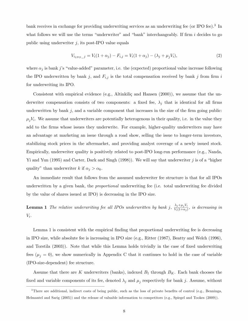
bank receives in exchange for providing underwriting services as an underwriting fee (or IPO fee).3 In

what follows we will use the terms “underwriter” and “bank” interchangeably. If firm i decides to go

public using underwriter j, its post-IPO value equals

ViIPO_j = Vi(1 + �j)� Fi,j = Vi(1 + �j)� (�j + µjVi), (2)

where �j is bank j’s “value-added” parameter, i.e. the (expected) proportional value increase following

the IPO underwritten by bank j, and Fi,j is the total compensation received by bank j from firm i

for underwriting its IPO.

Consistent with empirical evidence (e.g., Altinkiliç and Hansen (2000)), we assume that the un-

derwriter compensation consists of two components: a fixed fee, �j that is identical for all firms

underwritten by bank j, and a variable component that increases in the size of the firm going public:

µjVi. We assume that underwriters are potentially heterogenous in their quality, i.e. in the value they

add to the firms whose issues they underwrite. For example, higher-quality underwriters may have

an advantage at marketing an issue through a road show, selling the issue to longer-term investors,

stabilizing stock prices in the aftermarket, and providing analyst coverage of a newly issued stock.

Empirically, underwriter quality is positively related to post-IPO long-run performance (e.g., Nanda,

Yi and Yun (1995) and Carter, Dark and Singh (1998)). We will say that underwriter j is of a “higher

quality” than underwriter k if �j > �k.

An immediate result that follows from the assumed underwriter fee structure is that for all IPOs

underwritten by a given bank, the proportional underwriting fee (i.e. total underwriting fee divided

by the value of shares issued at IPO) is decreasing in the IPO size.

Lemma 1 The relative underwriting fee all IPOs underwritten by bank j, �j+µjViVi(1+�j)

, is decreasing in

Vi.

Lemma 1 is consistent with the empirical finding that proportional underwriting fee is decreasing

in IPO size, while absolute fee is increasing in IPO size (e.g., Ritter (1987), Beatty and Welch (1996),

and Torstila (2003)). Note that while this Lemma holds trivially in the case of fixed underwriting

fees (µj = 0), we show numerically in Appendix C that it continues to hold in the case of variable

(IPO-size-dependent) fee structure.

Assume that there are K underwriters (banks), indexed B1 through BK . Each bank chooses the

fixed and variable components of its fee, denoted �j and µj respectively for bank j. Assume, without

3There are additional, indirect costs of being public, such as the loss of private benefits of control (e.g., Benninga,

Helmantel and Sarig (2005)) and the release of valuable information to competitors (e.g., Spiegel and Tookes (2009)).

8

loss of generality, that �i � �j u i < j, i.e. that underwriters are sorted by quality from high to

low. The banks face increasing marginal costs of providing underwriting services. This assumption is

in line with Khanna, Noe and Sonti’s (2008) model of inelastic supply of labor in investment banking

and is consistent with empirical estimates of the shape of underwriters’ cost function (e.g., Altinkiliç

and Hansen (2000)). In particular, we assume that for underwriter j, the total cost of underwriting n

IPOs, TCj,n, is

TCj,n = cn2. (3)

The assumption of total cost that is quadratic and marginal cost that is linear in the number of IPOs

underwritten by a bank simplifies the solution considerably as it precludes any corner solutions in

which a bank chooses not to underwrite any IPOs.

After observing the fees charged by all underwriters, each firm can pursue one of K + 1 mutually

exclusive strategies: it may remain private or it may perform an IPO underwritten by one of the K

banks. Firm i’s maximized value, V Wi is, thus

V = sup{Vi,maxj(Vi(1 + �j)� (�j + µjVi)}. (4)

As discussed above, in this section, we present an analytical solution of the model under two

restrictive assumptions. First, we assume two underwriters: K = 2. Second, we assume that each bank

charges fixed underwriting fee (which may be di�erent across banks), �j, but no variable component,

µj = 0 u j. Appendix B presents a numerical solution of the model that relaxes the first assumption,

while in Appendix C we relax the second assumption.

2.2 Two underwriters

In the case of two potentially heterogenous underwriters (B1 and B2, �1 � �2) and zero variable un-

derwriting fees (µ1 = µ2 = 0), it follows from (4) that each firm’s optimal strategy can be summarized

as follows:

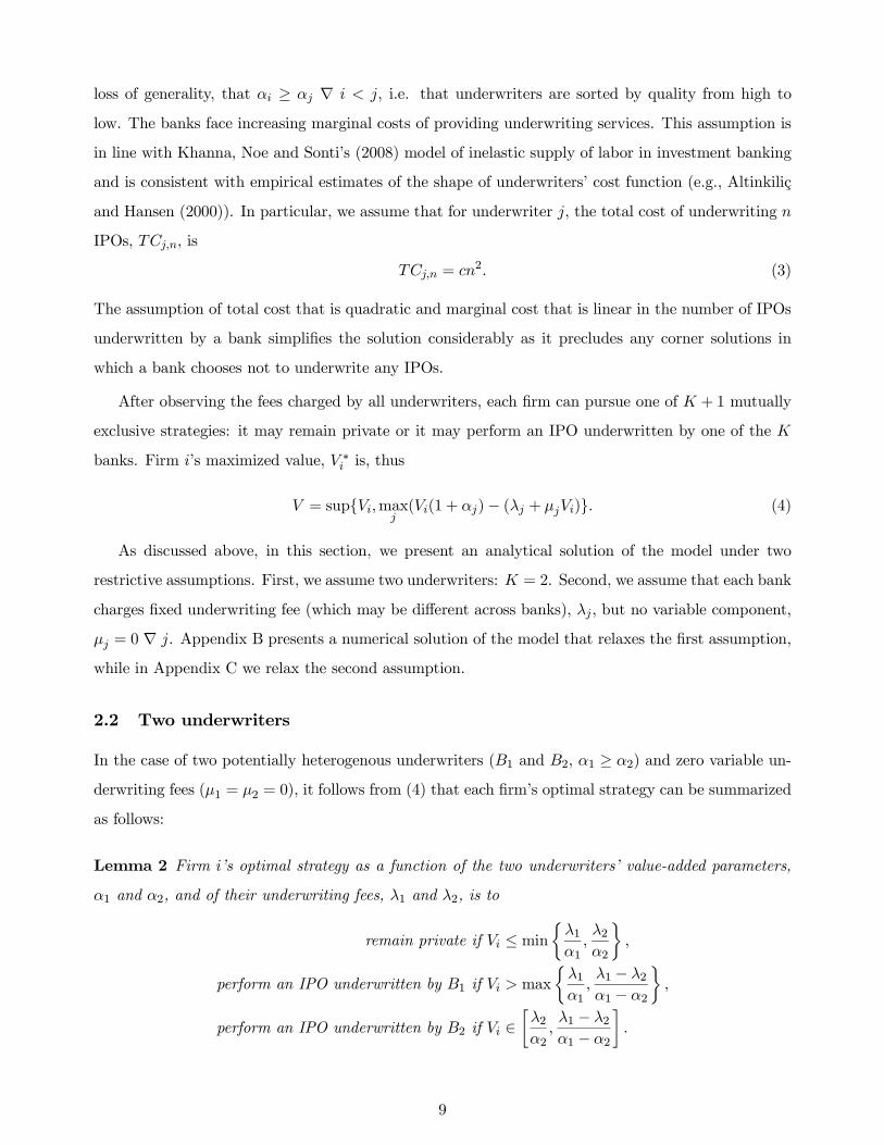
Lemma 2 Firm i’s optimal strategy as a function of the two underwriters’ value-added parameters,

�1 and �2, and of their underwriting fees, �1 and �2, is to

remain private if Vi � min��1�1,�2�2

�,

perform an IPO underwritten by B1 if Vi > max��1�1,�1 � �2�1 � �2

�,

perform an IPO underwritten by B2 if Vi 5��2�2,�1 � �2�1 � �2

�.

9

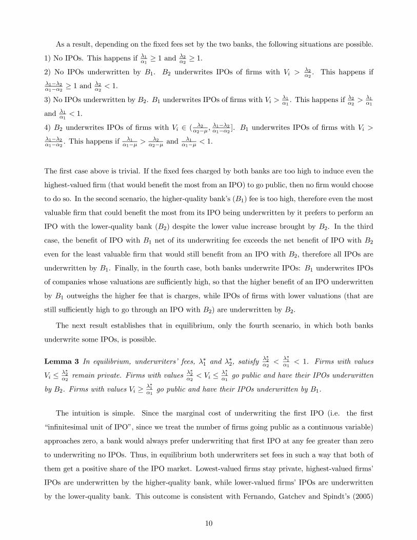
As a result, depending on the fixed fees set by the two banks, the following situations are possible.

1) No IPOs. This happens if �1�1� 1 and �2

�2� 1.

2) No IPOs underwritten by B1. B2 underwrites IPOs of firms with Vi > �2�2. This happens if

�13�2�13�2 � 1 and

�2�2< 1.

3) No IPOs underwritten by B2. B1 underwrites IPOs of firms with Vi > �1�1. This happens if �2

�2> �1

�1

and �1�1< 1.

4) B2 underwrites IPOs of firms with Vi 5 ( �2�23µ ,

�13�2�13�2 ]. B1 underwrites IPOs of firms with Vi >

�13�2�13�2 . This happens if

�1�13µ >

�2�23µ and

�1�13µ < 1.

The first case above is trivial. If the fixed fees charged by both banks are too high to induce even the

highest-valued firm (that would benefit the most from an IPO) to go public, then no firm would choose

to do so. In the second scenario, the higher-quality bank’s (B1) fee is too high, therefore even the most

valuable firm that could benefit the most from its IPO being underwritten by it prefers to perform an

IPO with the lower-quality bank (B2) despite the lower value increase brought by B2. In the third

case, the benefit of IPO with B1 net of its underwriting fee exceeds the net benefit of IPO with B2

even for the least valuable firm that would still benefit from an IPO with B2, therefore all IPOs are

underwritten by B1. Finally, in the fourth case, both banks underwrite IPOs: B1 underwrites IPOs

of companies whose valuations are su!ciently high, so that the higher benefit of an IPO underwritten

by B1 outweighs the higher fee that is charges, while IPOs of firms with lower valuations (that are

still su!ciently high to go through an IPO with B2) are underwritten by B2.

The next result establishes that in equilibrium, only the fourth scenario, in which both banks

underwrite some IPOs, is possible.

Lemma 3 In equilibrium, underwriters’ fees, �W1 and �W2, satisfy�W2�2<

�W1�1< 1. Firms with values

Vi ��W2�2remain private. Firms with values �W2

�2< Vi �

�W1�1go public and have their IPOs underwritten

by B2. Firms with values Vi ��W1�1go public and have their IPOs underwritten by B1.

The intuition is simple. Since the marginal cost of underwriting the first IPO (i.e. the first

“infinitesimal unit of IPO”, since we treat the number of firms going public as a continuous variable)

approaches zero, a bank would always prefer underwriting that first IPO at any fee greater than zero

to underwriting no IPOs. Thus, in equilibrium both underwriters set fees in such a way that both of

them get a positive share of the IPO market. Lowest-valued firms stay private, highest-valued firms’

IPOs are underwritten by the higher-quality bank, while lower-valued firms’ IPOs are underwritten

by the lower-quality bank. This outcome is consistent with Fernando, Gatchev and Spindt’s (2005)

10

assortative matching model of firms and underwriters, in which firm quality and underwriter quality

are positively correlated.

An immediate result that follows from Lemma 3 is that for a firm that is indi�erent between its

IPO underwritten by the two banks, the proportional fee of the higher-quality bank (B1) is higher

than that of the lower-quality bank (B2):

Lemma 4 If Vi =�W13�

W2

�13�2 ,�W1

Vi(1+�1)>

�W2Vi(1+�2)

.

In other words, ceteris paribus, an IPO that is underwritten by a higher-quality bank commands

higher proportional underwriting fee than an IPO that is underwritten by a lower-quality bank.

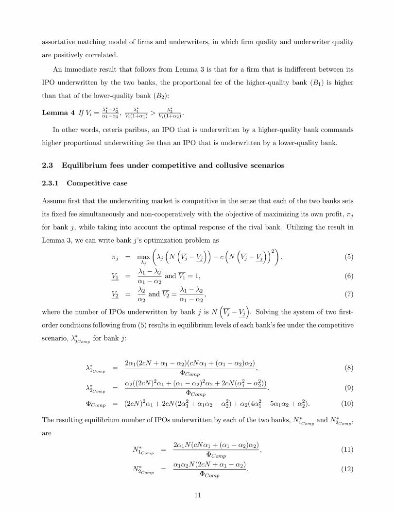
2.3 Equilibrium fees under competitive and collusive scenarios

2.3.1 Competitive case

Assume first that the underwriting market is competitive in the sense that each of the two banks sets

its fixed fee simultaneously and non-cooperatively with the objective of maximizing its own profit, �j

for bank j, while taking into account the optimal response of the rival bank. Utilizing the result in

Lemma 3, we can write bank j’s optimization problem as

�j = max�j

��j�N�Vj � Vj

��� c

�N�Vj � Vj

��2�, (5)

V1 =�1 � �2�1 � �2

and V1 = 1, (6)

V2 =�2�2

and V2 =�1 � �2�1 � �2

, (7)

where the number of IPOs underwritten by bank j is N�Vj � Vj

�. Solving the system of two first-

order conditions following from (5) results in equilibrium levels of each bank’s fee under the competitive

scenario, �WjComp for bank j:

�W1Comp =2�1(2cN + �1 � �2)(cN�1 + (�1 � �2)�2)

�Comp, (8)

�W2Comp =�2((2cN)2�1 + (�1 � �2)2�2 + 2cN(�21 � �22))

�Comp. (9)

�Comp = (2cN)2�1 + 2cN(2�21 + �1�2 � �22) + �2(4�

21 � 5�1�2 + �22). (10)

The resulting equilibrium number of IPOs underwritten by each of the two banks, NW1Comp and NW2Comp

,

are

NW1Comp =2�1N(cN�1 + (�1 � �2)�2)

�Comp, (11)

NW2Comp =�1�2N(2cN + �1 � �2)

�Comp. (12)

11

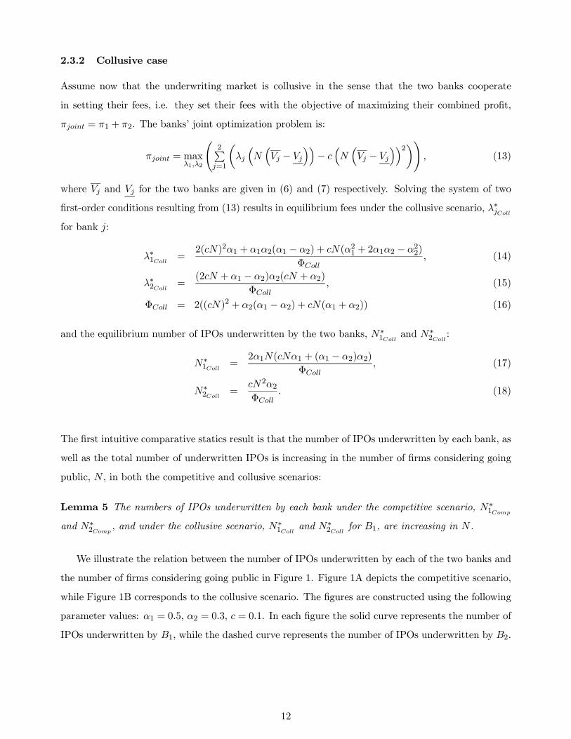
2.3.2 Collusive case

Assume now that the underwriting market is collusive in the sense that the two banks cooperate

in setting their fees, i.e. they set their fees with the objective of maximizing their combined profit,

�joint = �1 + �2. The banks’ joint optimization problem is:

�joint = max�1,�2

#2Sj=1

��j

�N�Vj � Vj

��� c

�N�Vj � Vj

��2�$, (13)

where Vj and Vj for the two banks are given in (6) and (7) respectively. Solving the system of two

first-order conditions resulting from (13) results in equilibrium fees under the collusive scenario, �WjColl

for bank j:

�W1Coll =2(cN)2�1 + �1�2(�1 � �2) + cN(�

21 + 2�1�2 � �22)

�Coll, (14)

�W2Coll =(2cN + �1 � �2)�2(cN + �2)

�Coll, (15)

�Coll = 2((cN)2 + �2(�1 � �2) + cN(�1 + �2)) (16)

and the equilibrium number of IPOs underwritten by the two banks, NW1Coll and NW2Coll

:

NW1Coll =2�1N(cN�1 + (�1 � �2)�2)

�Coll, (17)

NW2Coll =cN2�2�Coll

. (18)

The first intuitive comparative statics result is that the number of IPOs underwritten by each bank, as

well as the total number of underwritten IPOs is increasing in the number of firms considering going

public, N , in both the competitive and collusive scenarios:

Lemma 5 The numbers of IPOs underwritten by each bank under the competitive scenario, NW1Compand NW2Comp , and under the collusive scenario, N

W1Coll

and NW2Coll for B1, are increasing in N .

We illustrate the relation between the number of IPOs underwritten by each of the two banks and

the number of firms considering going public in Figure 1. Figure 1A depicts the competitive scenario,

while Figure 1B corresponds to the collusive scenario. The figures are constructed using the following

parameter values: �1 = 0.5, �2 = 0.3, c = 0.1. In each figure the solid curve represents the number of

IPOs underwritten by B1, while the dashed curve represents the number of IPOs underwritten by B2.

12

Figure 1: Number of IPOs as a function of the state of the IPO market

Figure 1A: Competitive case Figure 1B: Collusive case

The monotonic relation between the equilibrium number of IPOs and N in both the competitive and

collusive settings is useful because it enables translating various comparative statics of the model with

respect to N into empirical predictions regarding the relations between observable quantities in the

IPO market and the “hotness” of the market, i.e. the number of firms going public in a particular

time period. In what follows, we will refer to both N and the total number of IPOs, NW1Comp +NW2Comp

and NW1Coll +NW2Coll

, under the competitive and collusive scenarios respectively, which are monotonic

functions of N , as the state of the IPO market.

2.4 Comparative statics

We now turn to examining the comparative statics of the equilibria obtained under the two scenarios

with the objective of designing empirical tests of implicit underwriter collusion hypothesis against the

alternative of oligopolistic competition. We begin by examining the relations between the two banks’

equilibrium absolute and proportional underwriting fees and the state of the market and proceed to

analyze the relation between the banks’ equilibrium shares of the IPO market and the state of the

market.

2.4.1 Proportional underwriting fees

We define the weighted average proportional fee of bank j as the ratio of the combined fees collected

by bank j from all firms whose IPOs it underwrites to the combined pre-IPO value of these firms:

Definition 1 The weighted average proportional fee of bank j, RFj , equals

�Wj

�N�Vj3Vj

��+µWjN

VjU

V=Vj

V dV

N

VjU

V=Vj

V dV

or, in the case of zero variable fees,�Wj

�Vj3Vj

�

VjU

V=Vj

V dV

.

13

The relation between the two banks’ proportional fees and the state of the IPO market is summa-

rized in the following two propositions.

Proposition 1 In a competitive underwriting market, the weighted average proportional fee of the

higher-quality bank (B1) and that of the lower-quality bank (B2) are increasing in N .

The intuition behind the positive relation between the average proportional fees of the two banks

and the state of the IPO market in the competitive case is as follows. Because of the banks’ increasing

marginal costs, as the number of firms considering an IPO increases, the set of firms that the banks

choose to underwrite becomes more and more selective. This also means that the range of values of

firms underwritten by each of the banks narrows as N increases (i.e. as the state of the IPO market

improves). The proportional fee paid by the lowest-valued firm that the lower-quality bank (B2)

underwrites equals �2, since for that firm the bank extracts the whole surplus obtained at the time of

the IPO. As follows from Lemma 1, the proportional fee paid by a firm to a given bank is decreasing in

firm’s quality, thus the average proportional fee paid to B2 is lower than �2. However, since the range

of values of firms whose IPOs are underwritten by B2 is decreasing in N , the average proportional fee

approaches the highest proportional fee (�2) as N increases. While the higher-quality bank (B1) does

not extract the full surplus from the lowest-valued firm among those it underwrites (because that firm

has the option of its IPO being underwritten by B2 instead), similar logic holds for B1: the higher the

state of the IPO market, the narrower the range of values of firms underwritten by B1, implying that

the B1’s average proportional fee approaches the highest relative fee charged by B1 as N increases.

Proposition 2 In a collusive underwriting market:

a) the weighted average proportional fee of the higher-quality bank (B1) is increasing in N ;

b) the weighted average proportional fee of the lower-quality bank (B2) exhibits a U-shaped relation

with N : it is decreasing in N for su!ciently low N and it is increasing in N for su!ciently high N .

The intuition behind the positive relation between the average proportional fee of a higher-quality

bank and N in the collusive scenario is similar to that in the competitive scenario: higher N leads

to a smaller range of values of firms underwritten by the higher-quality bank, raising its average

proportional fee. The U-shaped relation between the average proportional fee of a lower-quality bank

and the state of the IPO market in the collusive case is a little more subtle, as it is driven by a

combination of two e�ects. First, as with the higher-quality bank, higher N leads to a smaller range

of values of firms underwritten by the lower-quality bank, raising its average proportional fee.

Second, for low levels of N , the two banks’ joint expected profit is maximized when most IPOs

are performed by B1. The reason is if banks collude with the objective of maximizing their combined

14

profit, then for low levels of N , for which the marginal cost structure is relatively flat, it is optimal

to channel most of the IPOs to the higher-quality bank that can charge a higher underwriting fee.

Allocating IPOs to the lower-quality bank would have a substantial negative e�ect on the number of

IPOs underwritten by the higher-quality bank, reducing the two banks’ combined profit. It is only

possible to channel most of the IPOs to the higher-quality bank by setting a high fee of the lower-

quality bank, leading to a decreasing relation between the lower-quality bank’s fee on one hand and

the state of the IPO market on the other hand in relatively low states of the IPO market.

As N increases, the higher-quality bank becomes constrained by its increasing marginal cost of

underwriting, making it optimal to allocate more IPOs to the lower-quality bank. Thus, when N is

high, the incentives to set high fees for the lower-quality bank are weaker, making the first (positive)

e�ect of the state of the IPO market on the lower-quality bank’s fee dominant. The combination of

these two e�ects leads to the U-shaped relation between the state of the IPO market and the average

proportional fee charged by the lower-quality underwriter.

We illustrate the relation between the weighted average proportional fees charged by each of the

two banks in Figure 2. Figure 2A corresponds to the competitive scenario, while Figure 2B represents

the collusive case. The figures are constructed using the same parameter values as in Figure 1.

In each figure the solid curve represents the average proportional fee of B1, while the dashed curve

represents the average proportional fee of B2. Consistent with propositions 1 and 2, both underwriters’

equilibrium proportional fees are increasing in the state of the IPO market in the competitive scenario,

whereas the relation between the state of the market and the equilibrium fee of the lower-quality

underwriter is U-shaped in the collusive scenario.

Figure 2: Banks’ proportional fees as a function of the state of the IPO market

Figure 2A: Competitive case Figure 2B: Collusive case

2.4.2 Absolute (dollar) underwriting fees

Next, we examine the relation between equilibrium absolute (dollar) fees charged by each of the two

banks and the state of the IPO market

15

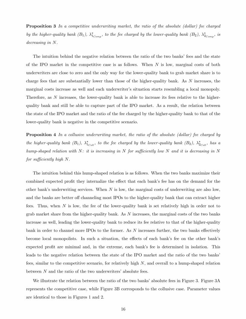
Proposition 3 In a competitive underwriting market, the ratio of the absolute (dollar) fee charged

by the higher-quality bank (B1), �W1Comp , to the fee charged by the lower-quality bank (B2), �W2Comp, is

decreasing in N .

The intuition behind the negative relation between the ratio of the two banks’ fees and the state

of the IPO market in the competitive case is as follows. When N is low, marginal costs of both

underwriters are close to zero and the only way for the lower-quality bank to grab market share is to

charge fees that are substantially lower than those of the higher-quality bank. As N increases, the

marginal costs increase as well and each underwriter’s situation starts resembling a local monopoly.

Therefore, as N increases, the lower-quality bank is able to increase its fees relative to the higher-

quality bank and still be able to capture part of the IPO market. As a result, the relation between

the state of the IPO market and the ratio of the fee charged by the higher-quality bank to that of the

lower-quality bank is negative in the competitive scenario.

Proposition 4 In a collusive underwriting market, the ratio of the absolute (dollar) fee charged by

the higher-quality bank (B1), �W1Coll , to the fee charged by the lower-quality bank (B2), �W2Coll

, has a

hump-shaped relation with N : it is increasing in N for su!ciently low N and it is decreasing in N

for su!ciently high N .

The intuition behind this hump-shaped relation is as follows. When the two banks maximize their

combined expected profit they internalize the e�ect that each bank’s fee has on the demand for the

other bank’s underwriting services. When N is low, the marginal costs of underwriting are also low,

and the banks are better o� channeling most IPOs to the higher-quality bank that can extract higher

fees. Thus, when N is low, the fee of the lower-quality bank is set relatively high in order not to

grab market share from the higher-quality bank. As N increases, the marginal costs of the two banks

increase as well, leading the lower-quality bank to reduce its fee relative to that of the higher-quality

bank in order to channel more IPOs to the former. As N increases further, the two banks e�ectively

become local monopolists. In such a situation, the e�ects of each bank’s fee on the other bank’s

expected profit are minimal and, in the extreme, each bank’s fee is determined in isolation. This

leads to the negative relation between the state of the IPO market and the ratio of the two banks’

fees, similar to the competitive scenario, for relatively high N , and overall to a hump-shaped relation

between N and the ratio of the two underwriters’ absolute fees.

We illustrate the relation between the ratio of the two banks’ absolute fees in Figure 3. Figure 3A

represents the competitive case, while Figure 3B corresponds to the collusive case. Parameter values

are identical to those in Figures 1 and 2.

16

Figure 3: Ratio of higher-quality bank’s absolute fee to that of lower-quality bank as a

function of the state of the IPO market

Figure 3A: Competitive case Figure 3B: Collusive case

2.4.3 Underwriters’ market shares

Proposition 5 In a competitive underwriting market

a) if the di�erence between the two banks’ qualities, �1 � �2 is su!ciently small, then the share of

IPOs underwritten by the higher-quality bank (B1),NW1Comp

NW1Comp+NW2Comp

, is decreasing in N ;

b) if the di�erence between the two banks’ qualities, �1��2 is su!ciently large, then the share of IPOs

underwritten by B1 is increasing in N .

The intuition for the results in Proposition 5 is as follows. When the two banks maximize their

separate expected profits from underwriting, the di�erence between the banks’ qualities is crucial in

determining the e�ects of the state of the IPO market on their market shares. When the di�erence

between the two underwriters’ qualities is relatively small, then in low states of the IPO market (i.e.

smallN).the competition between the two banks resembles Bertrand competition in homogenous goods

with close-to-zero marginal costs In such a situation, the market share of the higher-quality bank is

large.

In high states of the IPO market (i.e. large N), the situation resembles monopolistic competition

in which the two underwriters operate as local monopolists. This happens because in the presence

of increasing marginal costs of underwriting, as N becomes large, the higher-quality bank starts

underwriting only the highest-valued IPOs, while not challenging the lower-quality bank’s ability to

underwrite IPOs of lower-valued firms. In the extreme, each bank’s underwriting fee and the number of

IPOs each bank underwrites is determined by that bank in isolation of the optimal strategy of the other

bank. Thus, whenN is high, the ratio of the numbers of IPOs underwritten by the two banks converges

to the ratio of the numbers of IPOs at which each bank’s marginal costs of underwriting equals the

value added by that bank to the highest-valued firm. As a result, when the di�erence between the

17

two underwriters’ qualities is relatively small, the higher-quality (lower-quality) underwriter’s market

share is decreasing (increasing) in the state of the IPO market.

When the di�erence between the two banks’ qualities is relatively large, then in the low states of

the IPO market (i.e. close-to-zero marginal costs of underwriting), the only way for the lower-quality

underwriter to generate any revenues (and profits) is to charge lower underwriting fees and underwrite

more (low-valued) IPOs. As N increases, the marginal costs of underwriting increase as well, limiting

the ability of the lower-quality bank to charge low underwriting fees. This leads the lower-quality bank

to lose market share as the state of the IPO market improves and, as a result, to a positive (negative)

relation between the state of the IPO market and the higher-quality (lower-quality) bank’s share of

the market.

Proposition 6 In a collusive underwriting market the share of IPOs underwritten by the higher-

quality bank (B1),NW1Coll

NW1Coll+NW2Coll

, is decreasing in N .

As argued above, in the collusive scenario it is optimal to channel most IPOs to the higher-quality

bank in the low states of the IPO market, when the marginal costs of underwriting are relatively flat.

In higher states of the market the marginal costs of underwriting starts driving the allocation of IPOs

to the two banks, leading to an increased market share of the lower-quality bank. In the extreme,

when N $ 4, each bank underwrites only the highest-valued firms, and the only constraint on the

number of underwritten IPOs is the two banks’ marginal costs of underwriting. Thus, in the extreme,

each bank’s fee has no e�ect on the number of IPOs underwritten by the other bank, leading to more

equal equilibrium market shares as N becomes large. The resulting relation between the market share

of the higher-quality (lower-quality) bank and the state of the IPO market is negative (positive) under

the collusive scenario.

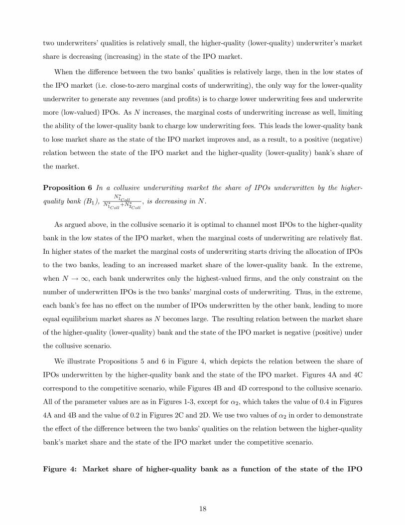
We illustrate Propositions 5 and 6 in Figure 4, which depicts the relation between the share of

IPOs underwritten by the higher-quality bank and the state of the IPO market. Figures 4A and 4C

correspond to the competitive scenario, while Figures 4B and 4D correspond to the collusive scenario.

All of the parameter values are as in Figures 1-3, except for �2, which takes the value of 0.4 in Figures

4A and 4B and the value of 0.2 in Figures 2C and 2D. We use two values of �2 in order to demonstrate

the e�ect of the di�erence between the two banks’ qualities on the relation between the higher-quality

bank’s market share and the state of the IPO market under the competitive scenario.

Figure 4: Market share of higher-quality bank as a function of the state of the IPO

18

market

Figure 4A: Competitive case, small �1 � �2 Figure 4B: Collusive case, small �1 � �2

Figure 4C: Competitive case, large �1 � �2 Figure 4D: Collusive case, large �1 � �2

The results in this section demonstrate that in a situation in which there are two underwriters,

the relation between these underwriters’ equilibrium fees and market shares on one side and the state

of the IPO market on the other side depend crucially on whether the underwriters implicitly collude

or compete. The comparative statics in the competitive and collusive scenarios lead to the following

empirical predictions.

2.5 Empirical predictions

2.5.1 Validation of the model setting

Before proceeding to test the collusion hypothesis against the alternative hypothesis of a competitive

underwriting market, it is possible to validate empirically the main assumptions of the model. Lemma

1 and also the extension of the model to the case in which both the fixed fee and relative fee are chosen

optimally in equilibrium, presented in Appendix C, leads to the following empirical prediction:

Prediction 1 For IPOs underwritten by a given bank, the proportional underwriting cost is expected

to be decreasing in the market value of shares issued at the time of the IPO.

Lemma 4 implies that controlling for IPO size, IPOs underwritten by higher-quality underwriters

are expected to be associated with higher proportional fees than those underwritten by lower-quality

underwriters.

19

Prediction 2 The proportional underwriting cost is expected to be higher for IPOs underwritten by

higher-quality banks, ceteris paribus.

While Predictions 1 and 2 enable partial validation of the model’s setup, the core empirical predictions

follow from the comparative statics under the competitive and collusive scenarios summarized in

Propositions 1-6. These predictions, which allow potentially test the implicit collusion hypothesis

against the alternative of competition among underwriters, are discussed in the next subsection.

2.5.2 Tests of the collusion and oligopolistic competition hypotheses

Propositions 1-2 result in empirical predictions regarding the e�ects of the state of the IPO market

on average proportional fee paid to underwriters.

Prediction 3a (Competition) Average proportional underwriter compensation is expected to be in-

creasing in the state of the IPO market.

Prediction 3b (Collusion) Average proportional underwriter compensation of low-quality under-

writers is expected to exhibit a U-shaped relation with the state of the IPO market. Average relative

underwriter compensation of higher-quality underwriters is expected to be increasing in the state of the

IPO market.

Propositions 3-4 lead to the empirical predictions regarding the e�ects of the state of the IPO market

on the ratio of dollar compensation paid to higher-quality underwriters to that paid to lower-quality

underwriters.

Prediction 4a (Competition) The ratio of average absolute (dollar) compensation paid to higher-

quality underwriters by firms whose IPOs they underwrite to the average compensation paid to lower-

quality underwriters is expected to be decreasing in the state of the IPO market.

Prediction 4b (Collusion) The ratio of average absolute (dollar) compensation paid to higher-quality

underwriters by firms whose IPOs they underwrite to the average compensation paid to lower-quality

underwriters is expected to have a hump-shaped relation with the state of the IPO market.

Propositions 5-6 lead to empirical predictions regarding the e�ects of the state of the IPO market

20

on the market share of higher-quality underwriters.

Prediction 5a (Competition) The market share of higher-quality underwriters are expected to be

decreasing in the state of the IPO market if the heterogeneity in underwriters’ qualities is relatively low

and it is expected to be increasing in the state of the IPO market if the heterogeneity in underwriters’

qualities is relatively high.

Prediction 5b (Collusion) The market share of higher-quality underwriters is expected to be de-

creasing in the state of the IPO market.

3 Empirical tests

3.1 Data

The IPO sample used in this paper is drawn from the Securities Data Company IPO database and

supplemented by data provided to us by Jay Ritter on IPO underwriting spreads, underwriter reputa-

tion scores, and on whether an IPO was syndicated and/or backed by venture capital funds. Following

prior studies examining underwriting fees and IPO underpricing (e.g., Chen and Ritter (2000), Hansen

(2001), and Abrahamson, Jenkinson and Jones (2011)), we exclude from our sample IPOs by banks,

closed-end funds, REITs, ADRs, unit o�erings, and o�erings that result from spino�s. Finally, to

include an IPO in our sample, we require that the information on underwriting spread and post-IPO

first-day return be available.

Our final sample consists of 6, 917 firm-commitment IPOs by U.S. firms between years 1975 and

2013. Panel A of Table 1 presents summary statistics of the IPO market by calendar year.

Insert Table 1 here

Columns 2 � 5 in Panel A contain annual statistics related to the state of the IPO market, stock

market, and the economy in general. The second column in Panel A of Table 1 shows that the number

of IPOs varies between 12 in 1975 and 603 in 1996. The third column presents IPO proceeds in

millions of dollars, adjusted by the Consumer Price Index (CPI) to 2010 dollars. In aggregate, U.S.

firms have raised over $600 billion (2010) dollars through IPOs during the 39 years of our sample.

Annual CPI-adjusted IPO proceeds also vary considerably throughout our sample period, from $501

million in 1977 to $44 billion in 2000. Early 1980s and the 1990s are the two hottest periods for IPOs.

The forth column reports the mean annual value-weighed market return in each of the 39 year of our

sample. Annual market returns range from �38% in 2002 to 37% in 1975, with an average of 13.8%.

21

The fifth column presents annual growth in private nonresidential fixed investment, which ranges from

�16% in 2009 to 21% is 1978. Overall, our sample includes periods of both hot and cold markets in

general and IPO markets in particular.

The next three columns present mean annual underwriting spreads and first post-IPO day an-

nouncement returns (aka underpricing). Similar to past studies (e.g., Chen and Ritter (2000) and

Hansen (2001)), the mean underwriting spread is 7.4%, and it has been on the declining trajectory

over the last three decades. The mean underpricing, calculated as the percentage di�erence between

the newly public stock’s closing price at the first trading day and its o�er price is 19%. Mean an-

nual underpricing varies over time, ranging from �0.2% for 12 IPOs underwritten in 1975 to 73%

for 397 IPOs underwritten in 1998. Consistent with past studies (e.g., Loughran and Ritter (2004)),

underpricing tends to be correlated with the hotness of IPO market: the correlation between mean

annual underpricing and the number of IPOs in that year is 45%. The next columns presents mean

underpricing, in which we replace negative first day returns with zeros.

The next four columns present annual IPO statistics. In particular, 40% of IPOs in our sample are

backed by venture capital funds, 46% of IPOs are by firms in the high-tech and/or biotech sector, 13%

of IPO proceeds are secondary, and 10% of IPOs are syndicated, i.e. involve multiple book runners.

The percentage of syndicated IPOs has been increasing over time — there were no syndicated IPOs up

to year 1991, while in each of the last five years of the sample more than 90% of IPOs are syndicated.

It is important to note that the fact that underwriters tend to form syndicates now much more than

in the past does not have to mean that they now collude more than previously in setting IPO fees.

While underwriters do set the fees jointly in IPOs that they underwrite jointly, collusion would imply

coordination of fees across IPOs, not within a single IPO.

In Panel B of Table 1 we report additional statistics for the variables described above. The

standard deviation of underwriting spread is about 1%, and the median is 7% exactly, consistent

with the clustering pattern documented by Chen and Ritter (2000). In contrast, there is a significant

variation in IPO underpricing. The standard deviation of underpricing across 6, 917 IPOs is 39%.

In our model, we show that the comparative statics of underwriter compensation with respect to

the state of the IPO market depends crucially on underwriter quality. Panel C of Table 1 presents

statistics on the number and volume of IPOs underwritten by banks of various qualities, as proxied

by the underwriter reputation score, first proposed by Carter and Manaster (1990) and extended by

Loughran and Ritter (2004). The highest score of 9 is given to fifteen most reputable underwriters

including Goldman Sachs, Morgan Stanley, Merrill Lynch, JP Morgan, Deutsche Bank, Citigroup, and

Credit Suisse. These banks underwrite one third of all deals in our sample in terms of numbers. Also,

22

IPOs underwritten by high-quality banks tend to be larger — there is an almost perfect monotonic

relation between the underwriter reputation score and the mean value of IPO proceeds, as follows

from the last column in Panel C.

3.2 Empirical tests

3.2.1 Model validation

We begin by testing Predictions 1 and 2 of the model, according to which the compensation for

underwriting an IPO is expected to be decreasing in the size of the IPO and is expected to be

increasing in the quality of the IPO underwriter. To test these predictions, we run a regression in

which the dependent variable is underwriter compensation, while the main independent variables are

IPO size and a measure of underwriter quality:

Compi,j,t = �+ �1HQi,t + �2IPO_sizej,t +�$���$Xi,t + Y earFEt + %i,t. (19)

Bank i’s proportional compensation for underwriting IPO of firm j in year t, Compi,j,t, consists

of a direct component and, possibly, an indirect one. The direct component is the underwriting fee

(gross spread) paid to the underwriter by the issuing firm. We consider a certain percentage of IPO

underpricing as the indirect component of underwriter’s compensation, following the evidence that

suggests that institutional investors in IPOs indirectly reward underwriters for profits they make in

the first day of aftermarket trading. For example, Reuter (2006) finds a positive relation between

trading commissions paid by a mutual fund family to an underwriter and the former’s holding of

recent profitable IPO shares allocated by that underwriter, and interprets his findings as underwriters

profiting from discretionary allocations of IPO shares. Nimalendran, Ritter, and Zhang (2007) find

abnormally intensive trading in the 50most liquid stocks before allocations of significantly underpriced

IPO shares and suggest that institutional investors trade liquid stocks to generate excessive commis-

sions to lead underwriters in order to get favorable allocations of underpriced IPO shares. Goldstein,

Irvine, and Puckett (2011) provide numerical estimates of the share of IPO underpricing that is re-

turned to underwriters in the form of increased trading commissions. While there is wide variation in

the proportion of underpricing captured by underwriters, Goldstein, Irvine and Puckett estimate that

on average lead underwriter receives between 2 and 5 cents in abnormal commission revenue for every

$1 left on the table.

We use two measures of underwriter compensation:

Direct_compi,j,t is the IPO spread. This measure may be understating the overall underwriter com-

pensation, but it is not plagued by problems in estimating the indirect component of compensation.

23

Direct&indirect_compi,j,t is the combination of IPO spread and a certain proportion of IPO un-

derpricing. Following Goldstein, Irvine and Puckett (2011), we use 5% of underpricing as a measure of

indirect compensation. (In cases in which underpricing is negative, we set it to zero.) The results are

robust to using other proportions of underpricing as a measure of indirect underwriter compensation,

such as 10%.

HQi,t is an indicator variable that equals one if underwriter i is of high quality in year t and

equals zero otherwise. According to Prediction 1, we expect to observe a positive coe!cient on the

higher-quality indicator, �1 > 0. We use two measures of underwriter quality:

CM_scorei,t is bank i’s Carter-Manaster (1990) reputation score, updated by Loughran and Rit-

ter (2004). In particular, if an underwriter’s score is 9 in a given year, it is defined as high-quality

underwriter in that year.4

Top_teni,t is based on bank i’s market share of the underwriting market, i.e. the proportion of

IPOs underwritten by bank i in year t out of all IPOs in year t. Specifically, high-quality underwriters

are those with top ten market shares.5 The correlation between the two measures of underwriter

quality is 59%.

IPO_sizej,t is measured as the natural logarithm of the issue proceeds, i.e. of the product of

the number of shares o�ered by firm j in its IPO and final o�er price. We use the logarithmic

transformation of IPO size because this variable exhibits high skewness. According to Prediction 2,

we expect that the coe!cient on IPO size be negative, �2 < 0.

We follow Hansen (2001), Torstila (2003), and Abrahamson, Jenkinson and Jones (2011) in defining

the vector of control variables, Xi,t, in (19). They include post-IPO 12-month daily stock return

volatility, the percentage of secondary shares in the o�ering, hi-tech dummy variable equaling one if

the issuing firm operates in the high-tech sector, where high-tech sector follows the SIC-code-based

definition in Loughran and Ritter (2004), VC dummy variable equaling one if the issue is backed by a

venture capital fund, and syndicate dummy that equals one if there are multiple book runners in the

issue.

We estimate the regression in (19) using OLS, while including year fixed e�ects and clustering

4Most of the results are robust to defining underwriters with Carter-Manaster scores of 8 and 9 as high-quality

underwriters.5The results are robust to defining top-five underwriters based on market share as high-quality ones.

24

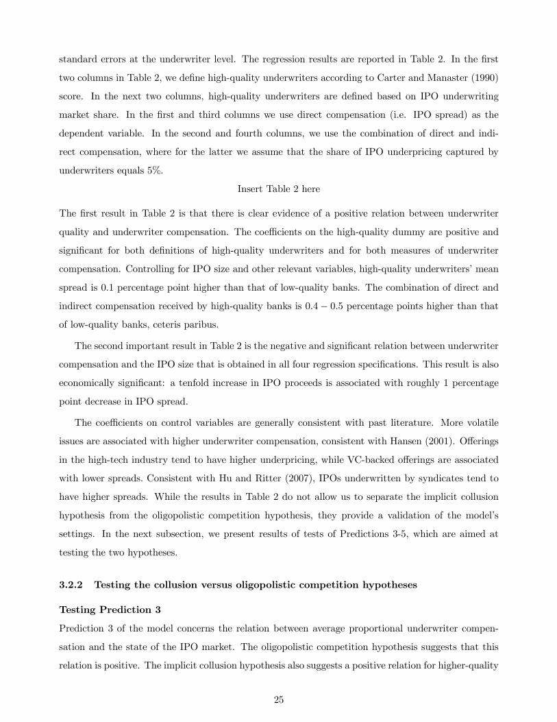
standard errors at the underwriter level. The regression results are reported in Table 2. In the first

two columns in Table 2, we define high-quality underwriters according to Carter and Manaster (1990)

score. In the next two columns, high-quality underwriters are defined based on IPO underwriting

market share. In the first and third columns we use direct compensation (i.e. IPO spread) as the

dependent variable. In the second and fourth columns, we use the combination of direct and indi-

rect compensation, where for the latter we assume that the share of IPO underpricing captured by

underwriters equals 5%.

Insert Table 2 here

The first result in Table 2 is that there is clear evidence of a positive relation between underwriter

quality and underwriter compensation. The coe!cients on the high-quality dummy are positive and

significant for both definitions of high-quality underwriters and for both measures of underwriter

compensation. Controlling for IPO size and other relevant variables, high-quality underwriters’ mean

spread is 0.1 percentage point higher than that of low-quality banks. The combination of direct and

indirect compensation received by high-quality banks is 0.4� 0.5 percentage points higher than that

of low-quality banks, ceteris paribus.

The second important result in Table 2 is the negative and significant relation between underwriter

compensation and the IPO size that is obtained in all four regression specifications. This result is also

economically significant: a tenfold increase in IPO proceeds is associated with roughly 1 percentage

point decrease in IPO spread.

The coe!cients on control variables are generally consistent with past literature. More volatile

issues are associated with higher underwriter compensation, consistent with Hansen (2001). O�erings

in the high-tech industry tend to have higher underpricing, while VC-backed o�erings are associated

with lower spreads. Consistent with Hu and Ritter (2007), IPOs underwritten by syndicates tend to

have higher spreads. While the results in Table 2 do not allow us to separate the implicit collusion

hypothesis from the oligopolistic competition hypothesis, they provide a validation of the model’s

settings. In the next subsection, we present results of tests of Predictions 3-5, which are aimed at

testing the two hypotheses.

3.2.2 Testing the collusion versus oligopolistic competition hypotheses

Testing Prediction 3

Prediction 3 of the model concerns the relation between average proportional underwriter compen-

sation and the state of the IPO market. The oligopolistic competition hypothesis suggests that this

relation is positive. The implicit collusion hypothesis also suggests a positive relation for higher-quality

25

underwriters, but for relatively low-quality underwriters it predicts a U-shaped relation. To test this

hypothesis we estimate the following regression:

Avg_compi,t = �+�1Mkt_statet�HQi,t+�2Mkt_statet�LQi,t+�3Mkt_state2t+�$���$Xi,t+%i,t. (20)

Avg_compi,t is the average compensation (direct and/or indirect) of underwriter i in year t. Mkt_statet

is the state of the IPO market. We use three measures of the IPO market state:

#IPOst is the annual number of IPOs underwritten in year t. This measure is motivated by the

model. As we show in Lemma 5, the equilibrium number of underwritten IPOs is increasing by the

state of the IPO market in the model, i.e. in the number of firms considering going public.

PNFI_grt is the annual growth in private nonresidential fixed investment (PNFI). Growth in PNFI

may be related to firms’ demand for capital (e.g., Lowry (2003), Pastor and Veronesi (2005), and

Yung, Çolak, and Wang (2008)) and resulting desire to raise funds using an IPO.

VW_mktrett is the value-weighted market return in year t. Firms are more likely to issue equity

in general and go public in particular in bull markets (e.g., Lucas and McDonald (1990), Lerner

(2004), and Ritter and Welch (2002).

HQi,t and LQi,t are high-quality and low-quality underwriter dummies, defined in the same way as in

the previous section, i.e. based on Carter-Manaster (1990) score or on the share of IPO underwriting

market. The control variables are the underwriter-year means of the control variables used in (19).

The regression in (20) is estimated at the underwriter-year level.

Both the implicit collusion and oligopolistic competition hypotheses predict a positive relation

between underwriter compensation and the state of the IPO market for high-quality underwriters.

Thus, both hypotheses predict that �1 � 0 and �3 > 0. However, the two hypotheses lead to di�erent

predictions for low-quality banks: the competition hypothesis predicts a positive relation between

underwriter compensation and the state of the IPO market, while the implicit collusion hypothesis

predicts a U-shaped relation. Hence, the important di�erence between the competition hypothesis and

the collusion hypothesis is that the former predicts that �2 � 0, while the latter predicts that �2 < 0.

Unlike (19), we do not include year fixed e�ects in (20), since we are interested in the association

between the state of the IPO market, which is measured on an annual basis, and average underwriter

compensation. Similar to (19), we cluster standard errors at the underwriter level. The results of

estimating (20) are reported in Table 3, which has 12 columns. In the first four columns #IPOst is

26

used at a measure of the state of the IPO market, in columns 5-8 we use PNFI_grt as a measure

of IPO market state, while in columns 9-12 we use VW_mktrett. In columns 1, 2, 5, 6, 9, and 10,

high-quality and low-quality underwriters are defined based on their Carter-Manaster (1990) scores,

while in columns 3, 4, 7, 8, 11, and 12, they are defined based on market shares. In odd columns only

direct underwriter compensation is considered, while in even columns we also account for estimated

indirect compensation.

Insert Table 3 here

The results for high-quality underwriters are generally consistent with both the competition and

collusion hypotheses: the coe!cient on Mkt_statet �HQi,t is generally insignificantly di�erent from

zero (it is significantly positive in two specifications out of twelve), while the coe!cient onMkt_state2t

is positive and significant in all twelve specifications. However, the important finding is that the results

for the low-quality underwriters support the implicit collusion hypothesis and are inconsistent with the

competition hypothesis: the coe!cients onMkt_statet �LQi,t are negative in all twelve specifications

and are statistically significant at the 5% level in ten of them, suggesting a U-shaped relation between

the state of the IPO market and compensation of lower-quality underwriters. The inflection points

of this U-shaped relation (i.e. � �22�3) ranges between 236 and 387 IPOs per year in columns 1 � 4,

between 9.7% and 12.6% annual PNFI growth in columns 5� 8, and between 5.7% and 12.7% annual

market return in columns 9� 12. All these values are in the range of the distributions of respective

measures of the state of the IPO market (although in the high end of this range in the case of #IPOst

and PNFI_grt), implying that the documented relation between the state of the IPO market and the

compensation of lower-quality underwriters is indeed U-shaped, consistent with the implicit collusion

hypothesis and inconsistent with the competition hypothesis.

Testing Prediction 4

Prediction 4 concerns the relation between the ratio of absolute (dollar) compensation received by

higher-quality underwriters to compensation received by lower-quality ones on one hand and the state

of the IPO market on the other hand. To test this prediction, we estimate the following regression:

log

�Avg_$CompiMHQ,tAvg_$CompLQ,t

�= �+ �1Mkt_statet + �2Mkt_state

2t +�$���$Xi,t + %i,t. (21)

The dependent variable in (21) is the natural logarithm of the ratio of the following two quantities.

The one in the numerator is the average dollar compensation of high-quality underwriter i in year

t, Avg_$CompiMHQ,t, computed as the mean dollar compensation per IPO, which in turn is the

product of proportional compensation, Compi,j,t, and IPO proceeds. The one in the denominator,

Avg_$CompLQ,t, is the average dollar compensation of low-quality underwriters in year t. We take

27

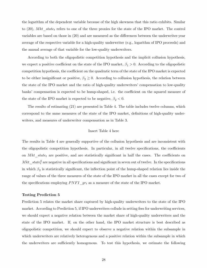
the logarithm of the dependent variable because of the high skewness that this ratio exhibits. Similar

to (20), Mkt_statet refers to one of the three proxies for the state of the IPO market. The control

variables are based on those in (20) and are measured as the di�erences between the underwriter-year

average of the respective variable for a high-quality underwriter (e.g., logarithm of IPO proceeds) and

the annual average of that variable for the low-quality underwriters.

According to both the oligopolistic competition hypothesis and the implicit collusion hypothesis,

we expect a positive coe!cient on the state of the IPO market, �1 > 0. According to the oligopolistic

competition hypothesis, the coe!cient on the quadratic term of the state of the IPOmarket is expected

to be either insignificant or positive, �2 � 0. According to collusion hypothesis, the relation between

the state of the IPO market and the ratio of high-quality underwriters’ compensation to low-quality

banks’ compensation is expected to be hump-shaped, i.e. the coe!cient on the squared measure of

the state of the IPO market is expected to be negative, �2 < 0.

The results of estimating (21) are presented in Table 4. The table includes twelve columns, which

correspond to the same measures of the state of the IPO market, definitions of high-quality under-

writers, and measures of underwriter compensation as in Table 3.

Insert Table 4 here

The results in Table 4 are generally supportive of the collusion hypothesis and are inconsistent with

the oligopolistic competition hypothesis. In particular, in all twelve specifications, the coe!cients

on Mkt_statet are positive, and are statistically significant in half the cases. The coe!cients on

Mkt_state2t are negative in all specifications and significant in seven out of twelve. In the specifications

in which �2 is statistically significant, the inflection point of the hump-shaped relation lies inside the

range of values of the three measures of the state of the IPO market in all the cases except for two of

the specifications employing PNFI_grt as a measure of the state of the IPO market.

Testing Prediction 5

Prediction 5 relates the market share captured by high-quality underwriters to the state of the IPO

market. According to Prediction 5, if IPO underwriters collude in setting fees for underwriting services,

we should expect a negative relation between the market share of high-quality underwriters and the

state of the IPO market. If, on the other hand, the IPO market structure is best described as

oligopolistic competition, we should expect to observe a negative relation within the subsample in

which underwriters are relatively heterogenous and a positive relation within the subsample in which

the underwriters are su!ciently homogenous. To test this hypothesis, we estimate the following

28

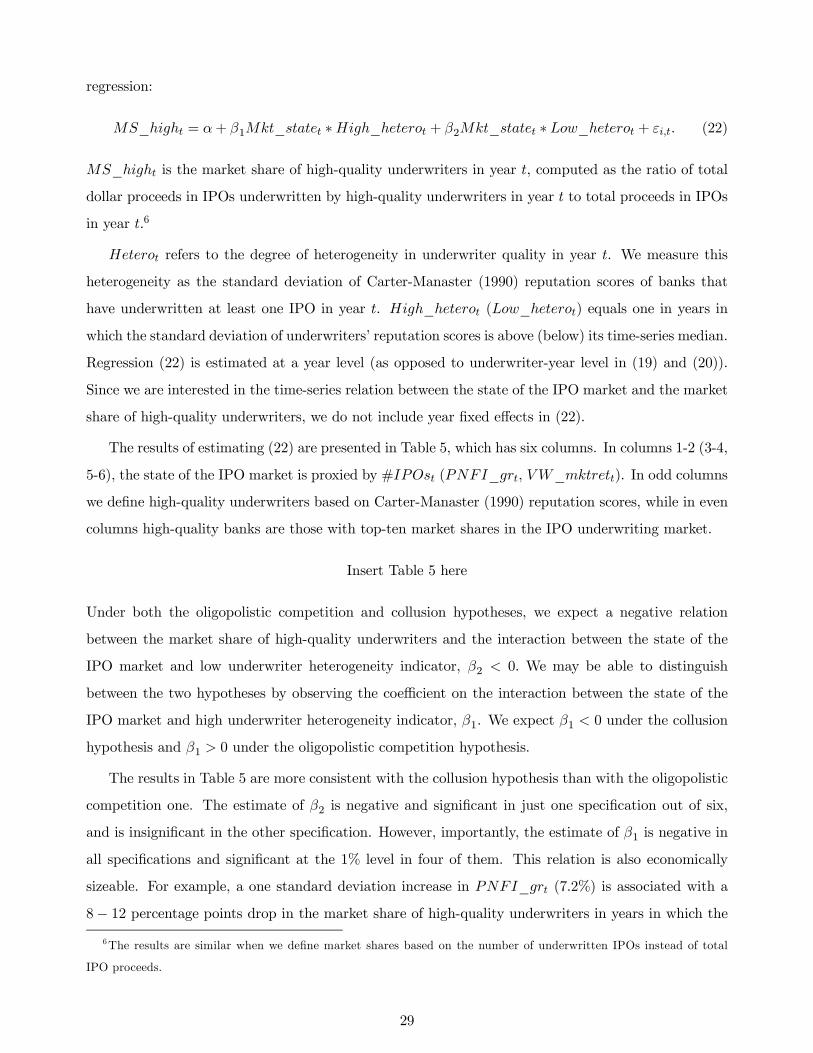
regression:

MS_hight = �+ �1Mkt_statet �High_heterot + �2Mkt_statet � Low_heterot + %i,t. (22)

MS_hight is the market share of high-quality underwriters in year t, computed as the ratio of total

dollar proceeds in IPOs underwritten by high-quality underwriters in year t to total proceeds in IPOs

in year t.6

Heterot refers to the degree of heterogeneity in underwriter quality in year t. We measure this

heterogeneity as the standard deviation of Carter-Manaster (1990) reputation scores of banks that

have underwritten at least one IPO in year t. High_heterot (Low_heterot) equals one in years in

which the standard deviation of underwriters’ reputation scores is above (below) its time-series median.

Regression (22) is estimated at a year level (as opposed to underwriter-year level in (19) and (20)).

Since we are interested in the time-series relation between the state of the IPO market and the market

share of high-quality underwriters, we do not include year fixed e�ects in (22).

The results of estimating (22) are presented in Table 5, which has six columns. In columns 1-2 (3-4,

5-6), the state of the IPO market is proxied by #IPOst (PNFI_grt, VW_mktrett). In odd columns

we define high-quality underwriters based on Carter-Manaster (1990) reputation scores, while in even

columns high-quality banks are those with top-ten market shares in the IPO underwriting market.

Insert Table 5 here

Under both the oligopolistic competition and collusion hypotheses, we expect a negative relation

between the market share of high-quality underwriters and the interaction between the state of the

IPO market and low underwriter heterogeneity indicator, �2 < 0. We may be able to distinguish

between the two hypotheses by observing the coe!cient on the interaction between the state of the

IPO market and high underwriter heterogeneity indicator, �1. We expect �1 < 0 under the collusion

hypothesis and �1 > 0 under the oligopolistic competition hypothesis.

The results in Table 5 are more consistent with the collusion hypothesis than with the oligopolistic

competition one. The estimate of �2 is negative and significant in just one specification out of six,

and is insignificant in the other specification. However, importantly, the estimate of �1 is negative in

all specifications and significant at the 1% level in four of them. This relation is also economically

sizeable. For example, a one standard deviation increase in PNFI_grt (7.2%) is associated with a

8� 12 percentage points drop in the market share of high-quality underwriters in years in which the

6The results are similar when we define market shares based on the number of underwritten IPOs instead of total

IPO proceeds.

29

heterogeneity in underwriter quality is high. This result is in line with the prediction of the collusion

hypothesis but is inconsistent with the competition hypothesis, which predicts positive �1.

Tests using a Subsample of Largest Underwriters

As mentioned above, it is conceivable that larger (higher-quality) underwriters collude among them-

selves but compete with smaller (lower-quality) underwriters. We show in Appendix B that the

predictions of our two models hold within a subset of colluding underwriters, even in the presence

of other, non-colluding, banks. In what follows, we examine empirically the predictions of the two

models while concentrating on a sample that consists of the largest ten underwriters in a given year,

with the idea that these banks are ex-ante more likely to collude among themselves than they are with

their smaller peers.

Table 6 reports results of re-estimating regressions reported in Tables 3—5 within the subsample of

the largest underwriters. While the set of control variables in the regressions in Table 6 are identical to

those in (20)—(22), to conserve space we do not report the coe!cients on control variables. In addition,

in Table 6 we report results using only one proxy for the state of the IPO market — the annual number

of IPOs.7 High-quality underwriters in Table 6 are defined di�erently than in Tables 3—5. In particular,

given that the vast majority of top-ten underwrites have a Carter-Manaster reputation score of 9, we

cannot use reputation score to define the highest-quality underwriters. Thus, we define underwriters

with the highest three (or highest five) market shares as those possessing the highest quality.

Insert Table 6 here

In Panel A, we re-estimate the regression in (20) for the sample of top-ten banks in each year. Sim-

ilar to the results in Table 3, the results for highest-quality underwriters are generally consistent with

both the competition and collusion hypotheses: the coe!cient on Mkt_statet �HQi,t is insignificant

in all specifications, while the coe!cient on Mkt_state2t is positive and significant in two specifi-

cations out of fore. Importantly, the results for the lower-quality underwriters are consistent with

the collusion hypothesis and are inconsistent with the competition hypothesis, as the coe!cients on

Mkt_statet �LQi,t are significantly negative in all four specifications, suggesting a U-shaped relation

between the state of the IPO market and lower-quality underwriters’ compensation.

Panel B reports estimates of the regression in (21) for the top-ten underwriter sample. The results

in Panel B are strongly supportive of the collusion hypothesis — more so than the full-sample results

in Table 4 — and are inconsistent with the competition hypothesis. In all four specifications, the

7The unreported results using the other two measures of the IPO market state — PNFI growth and value-weighted

market return — are generally similar to those reported in Table 6.

30

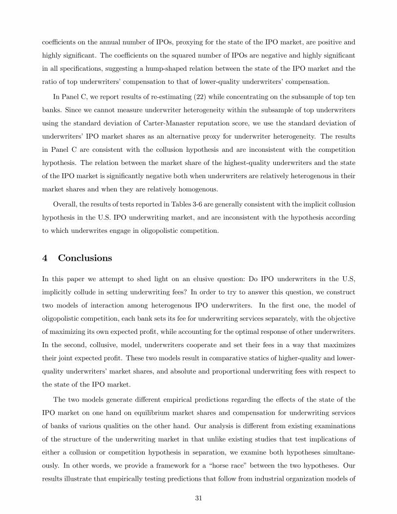
coe!cients on the annual number of IPOs, proxying for the state of the IPO market, are positive and

highly significant. The coe!cients on the squared number of IPOs are negative and highly significant

in all specifications, suggesting a hump-shaped relation between the state of the IPO market and the

ratio of top underwriters’ compensation to that of lower-quality underwriters’ compensation.

In Panel C, we report results of re-estimating (22) while concentrating on the subsample of top ten

banks. Since we cannot measure underwriter heterogeneity within the subsample of top underwriters

using the standard deviation of Carter-Manaster reputation score, we use the standard deviation of

underwriters’ IPO market shares as an alternative proxy for underwriter heterogeneity. The results

in Panel C are consistent with the collusion hypothesis and are inconsistent with the competition

hypothesis. The relation between the market share of the highest-quality underwriters and the state

of the IPO market is significantly negative both when underwriters are relatively heterogenous in their

market shares and when they are relatively homogenous.

Overall, the results of tests reported in Tables 3-6 are generally consistent with the implicit collusion

hypothesis in the U.S. IPO underwriting market, and are inconsistent with the hypothesis according

to which underwrites engage in oligopolistic competition.

4 Conclusions

In this paper we attempt to shed light on an elusive question: Do IPO underwriters in the U.S,

implicitly collude in setting underwriting fees? In order to try to answer this question, we construct

two models of interaction among heterogenous IPO underwriters. In the first one, the model of

oligopolistic competition, each bank sets its fee for underwriting services separately, with the objective

of maximizing its own expected profit, while accounting for the optimal response of other underwriters.

In the second, collusive, model, underwriters cooperate and set their fees in a way that maximizes

their joint expected profit. These two models result in comparative statics of higher-quality and lower-

quality underwriters’ market shares, and absolute and proportional underwriting fees with respect to

the state of the IPO market.

The two models generate di�erent empirical predictions regarding the e�ects of the state of the

IPO market on one hand on equilibrium market shares and compensation for underwriting services

of banks of various qualities on the other hand. Our analysis is di�erent from existing examinations

of the structure of the underwriting market in that unlike existing studies that test implications of

either a collusion or competition hypothesis in separation, we examine both hypotheses simultane-

ously. In other words, we provide a framework for a “horse race” between the two hypotheses. Our

results illustrate that empirically testing predictions that follow from industrial organization models of

31

interactions among underwriters and between underwriters and issuing firms and investors may lead

to better understanding of the competitive structure of the IPO underwriting market.

The competitive and collusive models result in several contrasting empirical predictions. We exploit

these di�erences in empirical implications and test the two models using data on U.S. IPOs from 1975

to 2013. Most of our evidence is consistent with the implicit collusion hypothesis, and it is mostly

inconsistent with the oligopolistic competition hypothesis. While beyond the scope of this paper,

it would be interesting to examine the model’s predictions using data from non-U.S. markets with

su!cient time-series IPO data, such as the U.K., Japan, and Canada, in order to test the claim

that non-U.S. underwriting markets are more competitive than the U.S. underwriting market (e.g.,

Abrahamson, Jenkinson and Jones (2011)).

32

5 Appendix

A Proofs

Proof of Lemma 1 Di�erentiating the proportional underwriting fee,�j+µjViVi(1+�j)

, with respect to Vi

results inC�j+µjViVi(1+�j)

CVi=

�jV 2i (1 + �j)

> 0. �

Proof of Lemma 2 Firm i’s value if private, Vi,private, is Vi. Firm i’s value after an IPO underwritten

by B1 or B2 is

Vi,IPO(B1) = Vi(1 + �1)� �1,

Vi,IPO(B2) = Vi(1 + �2)� �2.

Vi,private � Vi,IPO(B1) if Vi ��1�1. Vi,private � Vi,IPO(B2) if Vi �

�2�2. Thus, Vi,private � max{Vi,IPO(B1), Vi,IPO(B2)}

if Vi � min{�1�1 ,�2�2}. Vi,IPO(B1) � Vi,IPO(B2) if Vi �

�13�2�13�2 . Vi,IPO(B1) � Vi if Vi � �1

�1. Thus,

Vi,IPO(B1) � max{Vi,private, Vi,IPO(B2)} if Vi � max{�1�1, �13�2�13�2 }. Vi,IPO(B2) � Vi,IPO(B1) if Vi �

�13�2�13�2 .

Vi,IPO(B2) � Vi if Vi ��2�2. Thus, Vi,IPO(B2) � max{Vi,private, Vi,IPO(B1)} if Vi 5

k�2�2, �13�2�13�2

l. �

Proof of Lemma 3 The lowest-valued firm for which Vi,IPO(B2) > Vi,private is V2= �2�2. Assume

�1�1� �2

�2. Then for firm with value V2, Vi,IPO(B1) � Vi,IPO(B2), and Vi,IPO(B1) > Vi,IPO(B2) for any

Vi >V2. As a result, B2 would not underwrite any IPOs. Since the marginal cost of underwriting

the first infinitesimal unit of IPOs is zero, in equilibrium B2 would set �2 such that�W2�2<

�W1�1. The

highest-valued firm for which Vi,IPO(B1) > Vi,private is V1 = 1. Assume �1�1� 1. Then for firm with

value V1, Vi,private � Vi,IPO(B1), and Vi,private > Vi,IPO(B1) for any Vi < V1. As a result, B1 would not

underwrite any IPOs. Since the marginal cost of underwriting the first infinitesimal unit of IPOs is

zero, in equilibrium B1 would set �1 such that�W1�1< 1. �

Proof of Lemma 4 Since, according to Lemma 3, �W2�2<

�W1�1, and �1 � �2 by assumption, �W1 > �W2.

Therefore,�W1

�W13�W2

�13�2 (1 + �1)�

�W2�W13�

W2

�13�2 (1 + �2)=(�W1 � �W2) + (�

W1�2 � �W2�1)

�W13�W2

�13�2 (1 + �1)(1 + �2)> 0. �

33

Proof of Lemma 5 Di�erentiating NW1Comp , NW2Comp

, NW1Coll , and NW2Coll

in (11), (12), (17), and (18)

respectively with respect to N leads to

CNW1CompCN

=

2�1(N2�2c2�1

�2�21 + �22 � �1�2

�)�+N (2c�1�2 (�1 � �2) (4�1 � �2)) + (�

22 (4�1 � �2) (�1 � �2)

2))�4c2N2�1 + 4cN�21 + 2cN�1�2 + 4�21�2 � 2cN�22 � 5�1�22 + �32

�2 > 0,

CNW2CompCN

=

�1�2(N2�4c2(�21 � �22) + 8c

2�1�2�+N (4c�2 (�1 � �2) (4�1 � �2)) + �2 (4�1 � �2) (�1 � �2)

2)�4c2N2�1 + 4cN�21 + 2cN�1�2 + 4�21�2 � 2cN�22 � 5�1�22 + �32

�2 > 0,

CNW1CollCN

=N2c2(�21 + �22) + 2Nc�1�2(�1 � �2) + �22(�1 � �2)

2

2(c2N2 + cN�1 + cN�2 + �1�2 � �22)2

> 0,

CNW2CollCN

=Nc�2(Nc(�1 + �2) + 2�2(�1 � �2))

2(c2N2 + cN�1 + cN�2 + �1�2 � �22)2> 0.

It follows thatC�NW1Comp

+NW2Comp

�

CN > 0 andC�NW1Coll

+NW2Coll

�

CN > 0. �

Proof of Proposition 1 Weighted average proportional fees of B1 and B2 in the competitive

scenario, RF1Wand RF2

Win Definition 1 can be rewritten as

RF1compW=

2�1(2Nc+ �1 � �2)(Nc�1 + �2(�1 � �2))

(1 + �1)�N2(4c2�1) +N(3c�21 + 2c�1�2 � 2c�22) + (�2 (�1 � �2) (3�1 � �2))

� ,(23)

RF2compW=

2�2 (2Nc�1 + �2 (�1 � �2))

(1 + �2)�4Nc�1 + 3�1�2 � 2�22

� . (24)

Di�erentiating (23) and (24) with respect to N leads to

CRF1compW

CN=

2c�21�N2c2(2�21 + 4�

22) + 4Nc�2(c�

21 � c�22) + (3�22

��2 + �21 � 2�1�2

�)�

(1 + �1)�N2(4c2�1) +N(3c�21 + 2c�1�2 � 2c�22) + (�2 (�1 � �2) (3�1 � �2))

�2 > 0,

CRF2compW

CN=

4c�21�22

(1 + �2)�4Nc�1 + 3�1�2 � 2�22

�2 > 0. �

Proof of Proposition 2 Weighted average proportional fees of B1 and B2 in the collusive scenario,

RF1Wand RF2

Win Definition 1 can be rewritten as

RF1c ollW=

2�2N2c2�1 +N(c�

21 + 2c�1�2 � c�

22) + (�

21�2 � �1�

22)�

(1 + �1)(4N2c2 +N(3c�1 + 4c�2 � 2c�22) + 3�2 (�1 � �2)), (25)

RF2c ollW=

�2 (2Nc+ �1 � �2) (Nc+ �2)

(1 + �2) (4N2c2�1 +N(3c�1 + 4c�2) + 3�2 (�1 � �2)). (26)

Di�erentiating (25) and (26) with respect to N leads to

CRF1c ollW

CN=

2c�2N2c2(�21 + 2�

22) + 4Nc(�

21�2 � �1�

22) + (�

22 (2�1 � 3�2) (�1 � �2))

�

(1 + �1)(4N2c2 +N(3c�1 + 4c�2 � 2c�22) + 3�2 (�1 � �2))2> 0,

CRF2c ollW

CN=

2c�22�2N2c2 � �2 (�1 � �2)

�

(1 + �2) (4N2c2�1 +N(3c�1 + 4c�2) + 3�2 (�1 � �2))2 . (27)

The expression in (27) is positive for N >t

�2(�13�2)2c2

and is negative for N <t

�2(�13�2)2c2

. �

34

Proof of Proposition 3 Di�erentiating�W1Comp�W2Comp

with respect to N leads to

C

��W1Comp�W2Comp

�

CN= �

2c(�1 � �2)�21

(2Nc�1 + �2(�1 � �2))2 < 0. �

Proof of Proposition 4 Di�erentiating�W1Coll�W2Coll

with respect to N leads to

C��W1Coll�W2Coll

�

CN= �

c(�1 � �2)�2N2c2 � �2(�1 � �2)

�

(2Nc+ �1 � �2)2 (Nc+ �2)2

. (28)

The expression in (28) is positive for N <t

�2(�13�2)2c2

and is negative for N >t

�2(�13�2)2c2

. �

Proof of Proposition 5 Di�erentiatingNW1Comp

NW1Comp+NW2Comp

with respect to N leads to

C

�NW1Comp

NW1Comp+NW2Comp

�

CN=

2c(�1 � 2�2)(�1 � �2)�22Nc(�1 + �2) + 3�2(�1 � �2)

. (29)

The expression in (29) is positive for �1 > 2�2 and it is negative for �1 < 2�2. �

Proof of Proposition 6 Di�erentiatingNW1Coll

NW1Coll+NW2Coll

with respect to N leads to

C

�NW1Coll

NW1Coll+NW2Coll

�

CN= �

c(�1 � �2)�22

Nc(�1 + �2) + �2(�1 � �2)< 0. �

B Multiple banks

In this section we relax the assumption of two underwriters. Assume that there are K banks sorted by

their quality. Assume also that banks that belong to the set C collude, while others do not. Extending

the model to the case of multiple underwriters results in the following optimization problems of the

K banks:

E�j = max�j

��j�N�Vj � Vj

��� c

�N�Vj � Vj

��2�; Bj /5 C, (30)

E�joint = max�j , jMC

#SjMCC

��j�N�Vj � Vj

��� c

�N�Vj � Vj

��2�$, (31)

V1 =�1 � �2�1 � �2

and V1 = 1, (32)

Vj =�j � �j+1�j � �j+1

and Vj =�j31 � �j�j31 � �j

; 1 < j < K, (33)

VK =�K

�K � µand VK =

�K31 � �K�K31 � �K

. (34)

35

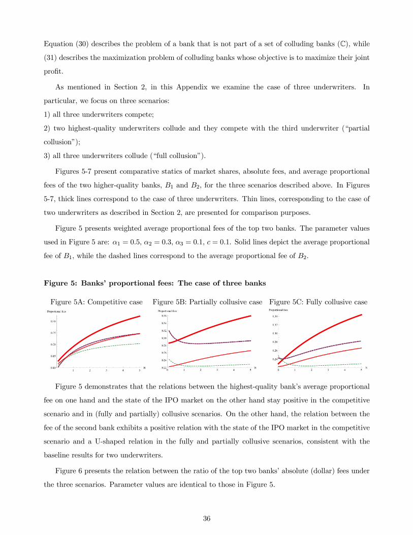
Equation (30) describes the problem of a bank that is not part of a set of colluding banks (C), while

(31) describes the maximization problem of colluding banks whose objective is to maximize their joint

profit.

As mentioned in Section 2, in this Appendix we examine the case of three underwriters. In

particular, we focus on three scenarios:

1) all three underwriters compete;

2) two highest-quality underwriters collude and they compete with the third underwriter (“partial

collusion”);

3) all three underwriters collude (“full collusion”).

Figures 5-7 present comparative statics of market shares, absolute fees, and average proportional

fees of the two higher-quality banks, B1 and B2, for the three scenarios described above. In Figures

5-7, thick lines correspond to the case of three underwriters. Thin lines, corresponding to the case of

two underwriters as described in Section 2, are presented for comparison purposes.

Figure 5 presents weighted average proportional fees of the top two banks. The parameter values

used in Figure 5 are: �1 = 0.5, �2 = 0.3, �3 = 0.1, c = 0.1. Solid lines depict the average proportional

fee of B1, while the dashed lines correspond to the average proportional fee of B2.

Figure 5: Banks’ proportional fees: The case of three banks

Figure 5A: Competitive case Figure 5B: Partially collusive case Figure 5C: Fully collusive case

Figure 5 demonstrates that the relations between the highest-quality bank’s average proportional

fee on one hand and the state of the IPO market on the other hand stay positive in the competitive

scenario and in (fully and partially) collusive scenarios. On the other hand, the relation between the

fee of the second bank exhibits a positive relation with the state of the IPO market in the competitive

scenario and a U-shaped relation in the fully and partially collusive scenarios, consistent with the

baseline results for two underwriters.

Figure 6 presents the relation between the ratio of the top two banks’ absolute (dollar) fees under

the three scenarios. Parameter values are identical to those in Figure 5.

36

Figure 6: Ratio of higher-quality bank’s to medium-quality bank’s absolute fees: The

case of three banks

Figure 6A: Competitive case Figure 6B: Partially collusive case Figure 6C: Fully collusive case

It follows from Figure 6 that, similar to the two-bank case, the relation between the ratio of the

two largest banks’ absolute fees and the state of the IPO market is negative when these two banks

compete and it exhibits a hump-shaped relation with N when the two banks collude, regardless of

whether they collude with the third bank or compete with the third bank.

Figure 7 presents the market share results. The market share of the highest-quality underwriter

(B1) depicted in Figure 5 is computed relative to the subset of the two highest-quality underwriters

that we consider to be more likely to potentially collude (i.e. B1 and B2). The parameter values in

Figure 7 are: �1 = 0.5, �3 = 0.1, c = 0.1. Similar to the case of two underwriters, we examine the case

in which the quality of the second underwriter is similar to that of the first underwriter (�2 = 0.4)

and the case in which �2 is substantially lower than �1 (�2 = 0.2).8

8The shape of the relations described in Figures 5-7 generally holds for various sets of parameter values that satisfy

�1 > �2 > �3.

37

Figure 7: Market share of higher-quality bank: The case of three banks

Figure 7A: Competitive case, Figure 7B: Partially collusive case, Figure 7C: Fully collusive case,

small �1 � �2 small �1 � �2 small �1 � �2

Figure 7D: Competitive case, Figure 7E: Partially collusive case, Figure 7F: Fully collusive case,

large �1 � �2 large �1 � �2 large �1 � �2

It follows from comparing the competitive case in Figures 7A and 7D with the partially and fully

collusive cases in Figures 7B, 7C, 7E, and 7F that in the case in which there is a large enough di�erence

between �1 and �2, the relation between the market share of the highest-quality bank and the state

of the IPO market is increasing in the competitive scenario and is decreasing when the top two banks

collude, regardless of whether they compete or collude with the third bank. When the di�erence

between �1 and �2 is relatively small, the relation between the market share of the highest-quality

underwriter and the state of the IPO market is negative in the competitive scenario and also in the

partially collusive and fully collusive scenarios.

Overall, the numerical analysis in this section demonstrates that the comparative statics in our

baseline model are unlikely to be driven by the assumption of two underwriters.

C Optimal variable underwriting fees

In this Appendix we solve numerically a model in which we allow each of the two underwriters to

choose not only its fixed fee, but also its variable fee, i.e. we now assume the following structure for

bank j’s fee: Fi,j = �j + µjVi.

For a given combination of �1, �2, µ1, and µ2 we compute using fine grid (of size G = 0.01) the

38

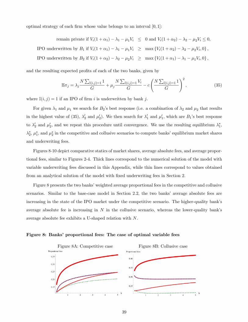
optimal strategy of each firm whose value belongs to an interval [0, 1]:

remain private if Vi(1 + �1)� �1 � µ1Vi � 0 and Vi(1 + �2)� �2 � µ2Vi � 0,

IPO underwritten by B1 if Vi(1 + �1)� �1 � µ1Vi � max {Vi(1 + �2)� �2 � µ2Vi, 0} ,

IPO underwritten by B2 if Vi(1 + �2)� �2 � µ2Vi � max {Vi(1 + �1)� �1 � µ1Vi, 0} ,

and the resulting expected profits of each of the two banks, given by

E�j = �jNSI(i,j)=1 1

G+ µj

NSI(i,j)=1 Vi

G� c

#NSI(i,j)=1 1

G

$2, (35)

where I(i, j) = 1 if an IPO of firm i is underwritten by bank j.

For given �1 and µ1 we search for B2’s best response (i.e. a combination of �2 and µ2 that results

in the highest value of (35), ��2 and µ�2). We then search for �

�1 and µ

�1, which are B1’s best response

to ��2 and µ�2, and we repeat this procedure until convergence. We use the resulting equilibrium �W1,

�W2, µW1, and µ

W2 in the competitive and collusive scenarios to compute banks’ equilibrium market shares

and underwriting fees.

Figures 8-10 depict comparative statics of market shares, average absolute fees, and average propor-

tional fees, similar to Figures 2-4. Thick lines correspond to the numerical solution of the model with

variable underwriting fees discussed in this Appendix, while thin lines correspond to values obtained

from an analytical solution of the model with fixed underwriting fees in Section 2.

Figure 8 presents the two banks’ weighted average proportional fees in the competitive and collusive

scenarios. Similar to the base-case model in Section 2.2, the two banks’ average absolute fees are

increasing in the state of the IPO market under the competitive scenario. The higher-quality bank’s

average absolute fee is increasing in N in the collusive scenario, whereas the lower-quality bank’s

average absolute fee exhibits a U-shaped relation with N .

Figure 8: Banks’ proportional fees: The case of optimal variable fees

Figure 8A: Competitive case Figure 8B: Collusive case

39

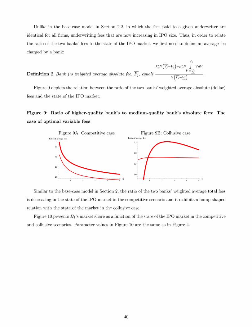
Unlike in the base-case model in Section 2.2, in which the fees paid to a given underwriter are

identical for all firms, underwriting fees that are now increasing in IPO size. Thus, in order to relate

the ratio of the two banks’ fees to the state of the IPO market, we first need to define an average fee

charged by a bank:

Definition 2 Bank j’s weighted average absolute fee, Fj, equals

�WjN�Vj3Vj

�+µWjN

VjU

V=Vj

V dV

N�Vj3Vj

� .

Figure 9 depicts the relation between the ratio of the two banks’ weighted average absolute (dollar)

fees and the state of the IPO market:

Figure 9: Ratio of higher-quality bank’s to medium-quality bank’s absolute fees: The

case of optimal variable fees

Figure 9A: Competitive case Figure 9B: Collusive case

Similar to the base-case model in Section 2, the ratio of the two banks’ weighted average total fees

is decreasing in the state of the IPO market in the competitive scenario and it exhibits a hump-shaped

relation with the state of the market in the collusive case.

Figure 10 presents B1’s market share as a function of the state of the IPO market in the competitive

and collusive scenarios. Parameter values in Figure 10 are the same as in Figure 4.

40

Figure 10: Market share of higher-quality bank: The case of optimal variable fees

.

Figure 10A: Competitive case: small �1 � �2 Figure 10B: Collusive case: small �1 � �2

Figure 10C: Competitive case: large �1 � �2 Figure 10D: Collusive case: large �1 � �2

As evident from Figure 10, the relations between banks’ market shares and the state of the IPO

market in the competitive and collusive scenarios are qualitatively similar to those in the zero-variable-

fees model in Section 2.2.

Overall, the results in this Appendix illustrate that introducing variable underwriting fees does

not a�ect the qualitative comparative statics derived in the baseline model.

41

References

Abrahamson, M., Jenkinson, T., and Jones, H., 2011, Why don’t U.S. issuers demand European feesfor IPOs, Journal of Finance 66, 2055-2082.

Allen, F., and Faulhaber, G., 1989, Signalling by underpricing in the IPOmarket, Journal of FinancialEconomics 23, 303-324.

Altinkiliç, O. and Hansen, R., 2000, Are there economies of scale in underwriting fees? Evidence ofrising external financing costs, Review of Financial Studies 13, 191-218.

Amihud, Y. and Mendelson, H., 1986, Asset pricing and the bid-ask spread, Journal of FinancialEconomics 17, 223—249.

Bain, J., 1951, Relationship of profit rate to industry concentration in American manufacturing1936-1940, Quarterly Journal of Economics, 65, 293—324.

Barla, P., 1998. Pricing and deregulation in the airline industry. In: Mayes, R., Gaudry, M. (Eds.),Taking Stock of Air Liberalization, Kluwer Academic Press, Ottawa.

Baron, D., 1982, A model of the demand for investment banking advising and distribution servicesfor new issues, Journal of Finance 37, 955-976.

Beatty, R., and Ritter, J., 1986, Investment banking, reputation, and the underpricing of initialpublic o�erings, Journal of Financial Economics 15, 213-232.

Beatty, R. and Welch, I., 1996, Issuer expenses and legal liability in initial public o�erings, Journalof Law and Economics 39, 545-602.

Benninga, S., Helmantel, M., and Sarig, O., 2005, The timing of initial public o�erings, Journal ofFinancial Economics 75, 115—132.

Benveniste, L., and Spindt, P., 1992, How investment banks determine the o�er price and allocationof new issues, Journal of Financial Economics 24, 343-362.

Bitler, M., Moskowitz, T., and Vissing-Jørgensen, A., 2005, Testing agency theory with entrepreneure�ort and wealth, Journal of Finance 60, 539—576.

Brau, J., and Fawcett, S., 2006, Initial public o�erings: An analysis of theory and practice, Journalof Finance 61, 399-436.

Carter, R., Dark, F., and Singh, A., 1998, Underwriter reputation, initial returns, and the long-runperformance of IPO stocks, Journal of Finance 53, 285—311.

Carter, R., and Manaster, S., 1990, Initial public o�erings and underwriter reputation, Journal ofFinance 45, 1045-1068.

Chemmanur, T., and Fulghieri, P., 1994, Investment bank reputation, information production, andfinancial intermediation, Journal of Finance 49, 57-79.

Chen, H. and Ritter, J., 2000, The seven percent solution, Journal of Finance 55, 1105—1131.

Chod, J. and Lyandres, E., 2011, Strategic IPOs and product market competition, Journal of Finan-cial Economics 100, 45-67.

Derrien, F. and Kecskés, A., 2007, The initial public o�erings of listed firms, Journal of Finance 62,447—479.

42

Dixit, A. and Stiglitz, J., 1977, Monopolistic competition and optimal product diversity, AmericanEconomic Review 67, 297—308.

Dunbar, C., 2000, Factors a�ecting investment bank initial public o�ering market share, Journal ofFinancial Economics 55, 3-41.

Fernando, C., Gatchev, V., and Spindt, P., 2005, Wanna dance? How firms and underwriters chooseeach other, Journal of Finance 60, 2437-2469.

Goldstein, M., Irvine, P., and Puckett, A., 2011, Purchasing IPOs with commissions, Journal ofFinancial and Quantitative Analysis 46, 1193-1225.

Gomes, A., 2000, Going public without governance: Managerial reputation e�ects, Journal of Finance55, 615—646.

Hansen, R., 2001, Do investment banks compete in IPOs? The advent of the “7% plus contract”,Journal of Financial Economics 59, 313—346.

Holmström, B. and Tirole, J., 1993, Market liquidity and performance monitoring, Journal of PoliticalEconomy 101, 678—709.

Hsieh, J., Lyandres, E., and Zhdanov, A., 2011, A theory of merger-driven IPOs, Journal of Financialand Quantitative Analysis 46, 1367-1405.

Hsu, H., Reed, A., and Rocholl, J., 2010, The new game in town: Competitive e�ects of IPOs,Journal of Finance 65, 495—528.

Hu, W., and Ritter, J., 2007, Multiple bookrunners in IPOs, University of Florida working paper.

Khanna, N., Noe, T., and Sonti, R., 2008, Good IPOs draw in bad: Inelastic banking capacity andhot markets, Review of Financial Studies 21, 1803-1906.

Krigman, L., Shaw, W., and Womack, K., 2001, Why do firms switch underwriters, Journal ofFinancial Economics 60, 245-284.

Lerner, J., 1994, Venture capitalists and the decision to go public, Journal of Financial Economics35, 293—316.

Liu, X., and Ritter, J., 2011, Local underwriter oligopolies and IPO underpricing, Journal of FinancialEconomics 102, 579-601.

Ljungqvist, A., and Wilhelm J., 2003, IPO pricing in the dot-com bubble, Journal of Finance 58,723—752.

Loughran, T., and Ritter, J., 2002, Why don’t issuers get upset about leaving money on the table inIPOs, Review of Financial Studies 15, 413—444.

Loughran, T., and Ritter, J., 2004, Why has IPO underpricing change over time?, Financial Man-agement 33, 5-37.

Loury, G., 1979, Market structure and innovation, Quarterly Journal of Economics 93, 395—410.

Lowry, M., 2003, Why does IPO volume fluctuate so much?, Journal of Financial Economics 67,3-40.

Lowry, M., and Schwert, W., 2002, IPO market cycles: Bubbles or sequential learning, Journal ofFinance 57, 1171-1200.

43

Lucas, D., and McDonald, R., 1990, Equity issues and stock price dynamics, Journal of Finance 45,1019—1043.

Mankiw, G. and Whinston, M., 1986, Free entry and social ine!ciency, RAND Journal of Economics17, 48—58.

Nanda, V., Yi, J., and Yun, Y., 1995, IPO long run performance and underwriter reputation, Un-published working paper, University of Michigan.

Nimalendran, M., Ritter, J., and Zhang, D., 2007, Do today’s trades a�ect tomorrow’s IPO alloca-tions?, Journal of Financial Economics 84, 87-109.

Okuguchi, K., 1973, Quasi-competitiveness and Cournot oligopoly, Review of Economic Studies 40,145—148.

Pastor, L. and Veronesi, P., 2005, Rational IPO waves, Journal of Finance 60, 1713-1754.

Reuter, J., 2006, Are IPO allocations for sale? Evidence from mutual funds, Journal of Finance 61,2289-2324.

Ritter, J., 1987, The costs of going public, Journal of Financial Economics 19, 269-281.

Ritter, J., 2011, Equilibrium in the IPO market, Annual Review of Financial Economics 3, 347-374.

Ritter, J., and Welch, I., 2002, IPO activity, pricing, and allocations, Journal of Finance 57, 1795-1828.

Rock, K., 1986, Why new issues are underpriced, Journal of Financial Economics 15, 187-212.

Rothschild, M. and Stiglitz, J., 1971, Increasing risk II: its economic consequences, Journal of Eco-nomic Theory 3, 66—84.

Ru!n, R., 1971, Cournot oligopoly and competitive behaviour, Review of Economic Studies 38,493—502.

Seade, J., 1980, On the e�ects of entry, Econometrica 48, 479—489

Shah, S. and Thakor, A., 1988, Private versus public ownership: investment, ownership distribution,and optimality, Journal of Finance 43,41—59.

Spiegel, M. and Tookes, H., 2009, Dynamic competition, innovation and strategic financing, Unpub-lished working paper, Yale University.

Suzumura, K. and Kiyono, K., 1987, Entry barriers and economic welfare, Review of EconomicStudies 54, 157—167.

Torstila, S., 2003, The clustering of IPO gross spreads: International evidence, Journal of Financialand Quantitative Analysis 38, 673-694.

von Weizsacker, C., 1980, A welfare analysis of barriers to entry, Bell Journal of Economics 11,399—420.

Welch, I., 1989, Seasoned o�erings, imitation costs, and the underpricing of initial public o�erings,Journal of Finance 44, 421-450.

Welch, I., 1992, Sequential sales, learning, and cascades, Journal of Finance 47, 695-732.

44

Yung, C., Çolak, G., and Wang, W., 2008, Cycles in the IPO market, Journal of Financial Economics89, 192-208.

Zingales, L., 1995, Insider ownership and the decision to go public, Review of Economic Studies 62,425—448.

45

Table 1. Summary statistics

Panel A reports annual means for the sample of IPOs used in the empirical tests. The sample consists of 6,917 IPOsby U.S. firms during 1975-2013. The source of data is Thomson Financial’s Security Data company and Jay Ritter. Thesample excludes non-firm-commitment o↵erings, unit o↵erings, o↵erings by banks, closed-end funds, REITs, and ADRs, ando↵erings that are a part of a corporate spino↵. We also require the IPOs to have information of underwriting spread andtotal proceeds. Number IPOs is the number of IPOs in a given year. IPO proceeds (in millions of dollars) are adjusted byConsumer Price Index (CPI) to 2010 dollars. Market return is the value-weighted annual market return. PNFI growth is theyear-to-year growth in private nonresidential fixed investment. Mean spread refers to equally-weighted mean underwriter’sfee divided by the size of the o↵ering (o↵er proceeds), which, in turn, equals the product of shares issued and o↵er price.Mean underpricing refers to equally-weighted mean ratio of the share price at the end of the first trading day and the o↵erprice, minus one. Mean underpricing (> 0) refers to equally-weighted mean underpricing, where negative underpricing issubstituted by 0. Prop. VC is the proportion of IPOs backed by venture capital funds. Prop hi-tech is the proportion ofIPOs in hi-tech industries. Prop. secondary is the equally-weighted mean proportion of secondary shares in IPOs. Prop.syndicated is the proportion of IPOs underwritten by multiple book runners.

Panel B presents descriptive statistics for the whole sample.

Panel C presents summary statistics of IPO underpricing for groups of underwriters classified by their reputation score(CM score), due to Carter and Manaster (1990) and Loughran and Ritter (2004). If an IPO has joint book runners (676deals in our sample involve two to eleven joint book runners), we divide its proceeds evenly by the number of book runnersand count this IPO multiple times in the analysis below.

46

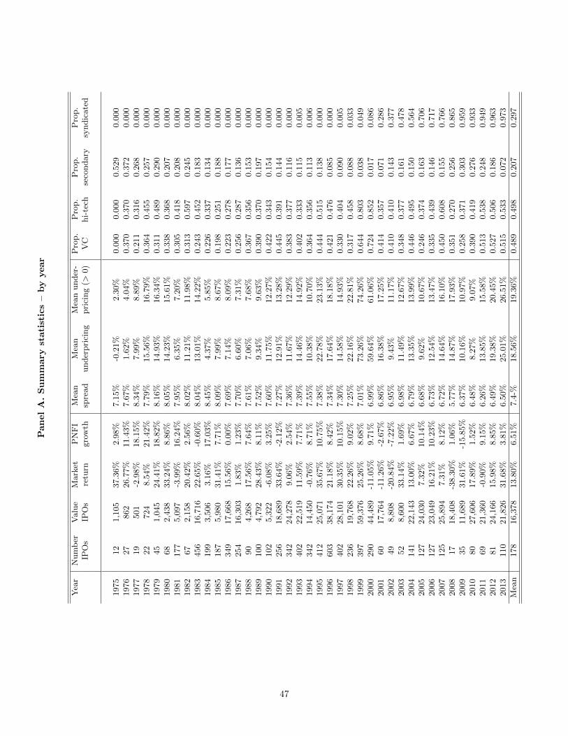
Panel

A.Summary

statistics–byyea

r

Year

Number

Value

Market

PNFI

Mean

Mean

Meanunder-

Prop.

Prop.

Prop.

Prop.

IPOs

IPOs

return

grow

thspread

underpricing

pricing(>

0)VC

hi-tech

secondary

syndicated

1975

121,10

537

.36%

2.98

%7.15

%-0.21%

2.30

%0.00

00.00

00.52

90.00

019

7627

862

26.77%

11.43%

7.67

%1.62

%4.04

%0.37

00.37

00.37

20.00

019

7719

501

-2.98%

18.15%

8.34

%7.99

%8.89

%0.21

10.31

60.26

80.00

019

7822

724

8.54

%21

.42%

7.79

%15

.56%

16.79%

0.36

40.45

50.25

70.00

019

7945

1,04

524

.41%

18.82%

8.16

%14

.93%

16.34%

0.31

10.48

90.29

00.00

019

8068

2,43

833

.24%

8.86

%8.05

%14

.23%

15.61%

0.33

80.36

80.20

70.00

019

8117

75,09

7-3.99%

16.24%

7.95

%6.35

%7.20

%0.30

50.41

80.20

80.00

019

8267

2,15

820

.42%

2.56

%8.02

%11

.21%

11.98%

0.31

30.59

70.24

50.00

019

8345

616

,716

22.65%

-0.60%

8.04

%13

.01%

14.22%

0.24

30.45

20.18

30.00

019

8419

93,50

63.16

%17

.03%

8.45

%4.37

%5.85

%0.22

60.33

70.13

40.00

019

8518

75,98

031

.41%

7.71

%8.09

%7.99

%8.67

%0.19

80.25

10.18

80.00

019

8634

917

,668

15.56%

0.00

%7.69

%7.14

%8.09

%0.22

30.27

80.17

70.00

019

8725

416

,303

1.83

%1.23

%7.70

%6.60

%7.31

%0.25

60.28

70.13

60.00

019

8890

4,26

817

.56%

7.64

%7.61

%7.06

%7.68

%0.36

70.35

60.15

30.00

019

8910

04,79

228

.43%

8.11

%7.52

%9.34

%9.63

%0.39

00.37

00.19

70.00

019

9010

25,32

2-6.08%

3.25

%7.60

%11

.75%

12.27%

0.42

20.34

30.15

40.00

019

9125

618

,689

33.64%

-2.12%

7.27

%12

.91%

13.28%

0.44

50.39

10.14

40.00

019

9234

224

,278

9.06

%2.54

%7.36

%11

.67%

12.29%

0.38

30.37

70.11

60.00

019

9340

222

,519

11.59%

7.71

%7.39

%14

.46%

14.92%

0.40

20.33

30.11

50.00

519

9434

214

,450

-0.76%

8.71

%7.55

%10

.38%

10.70%

0.36

40.35

60.11

30.00

619

9541

225

,071

35.67%

10.75%

7.38

%22

.78%

23.13%

0.44

40.51

50.13

80.00

019

9660

338

,174

21.18%

8.42

%7.34

%17

.64%

18.18%

0.42

10.47

60.08

50.00

019

9740

228

,101

30.35%

10.15%

7.30

%14

.58%

14.93%

0.33

00.40

40.09

00.00

519

9823

619

,768

22.26%

9.02

%7.25

%22

.16%

22.81%

0.31

70.45

80.08

80.03

319

9939

759

,376

25.26%

8.68

%7.01

%73

.26%

74.26%

0.64

40.80

30.03

80.04

920

0029

044

,489

-11.05

%9.71

%6.99

%59

.64%

61.06%

0.72

40.85

20.01

70.08

620

0160

17,764

-11.26

%-2.67%

6.86

%16

.38%

17.25%

0.41

40.35

70.07

10.28

620

0249

8,80

8-20.84

%-7.22%

6.95

%9.43

%11

.17%

0.41

00.41

00.14

30.37

720

0352

8,60

033

.14%

1.69

%6.98

%11

.49%

12.67%

0.34

80.37

70.16

10.47

820

0414

122

,143

13.00%

6.67

%6.79

%13

.35%

13.99%

0.44

60.49

50.15

00.56

420

0512

724

,030

7.32

%10

.14%

6.68

%9.62

%10

.67%

0.24

60.37

40.16

30.70

620

0612

723

,049

16.21%

10.23%

6.73

%12

.54%

13.47%

0.33

50.43

90.14

60.71

720

0712

525

,894

7.31

%8.12

%6.72

%14

.64%

16.10%

0.45

00.60

80.15

50.76

620

0817

18,408

-38.30

%1.06

%5.77

%14

.87%

17.93%

0.35

10.27

00.25

60.86

520

0935

11,689

31.61%

-15.85

%6.37

%10

.16%

10.97%

0.25

80.37

10.30

30.95

920

1080

27,606

17.89%

1.52

%6.48

%8.27

%9.07

%0.39

00.41

90.27

60.93

320

1169

21,360

-0.90%

9.15

%6.26

%13

.85%

15.58%

0.51

30.53

80.24

80.94

920

1281

24,166

15.98%

8.85

%6.49

%19

.38%

20.45%

0.52

70.50

60.18

60.96

320

1311

021

,826

31.68%

3.81

%6.50

%25

.01%

26.51%

0.51

50.53

30.07

20.97

3Mean

178

16,378

13.80%

6.51

%7.4-%

18.56%

19.36%

0.48

90.49

80.20

70.29

7

47

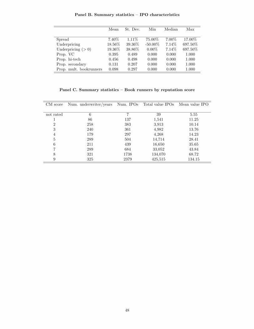
Panel B. Summary statistics – IPO characteristics

Mean St. Dev. Min Median Max

Spread 7.40% 1.11% 75.00% 7.00% 17.00%Underpricing 18.56% 39.36% -50.00% 7.14% 697.50%Underpricing (> 0) 19.36% 38.86% 0.00% 7.14% 697.50%Prop. VC 0.395 0.489 0.000 0.000 1.000Prop. hi-tech 0.456 0.498 0.000 0.000 1.000Prop. secondary 0.131 0.207 0.000 0.000 1.000Prop. mult. bookrunners 0.098 0.297 0.000 0.000 1.000

Panel C. Summary statistics – Book runners by reputation score

CM score Num. underwriter/years Num. IPOs Total value IPOs Mean value IPO

not rated 6 7 39 5.551 86 137 1,541 11.252 258 383 3,913 10.143 240 361 4,982 13.764 179 297 4,268 14.235 289 504 14,714 28.416 211 439 16,650 35.657 289 684 33,052 43.848 321 1738 134,070 68.729 325 2379 425,515 134.15

48

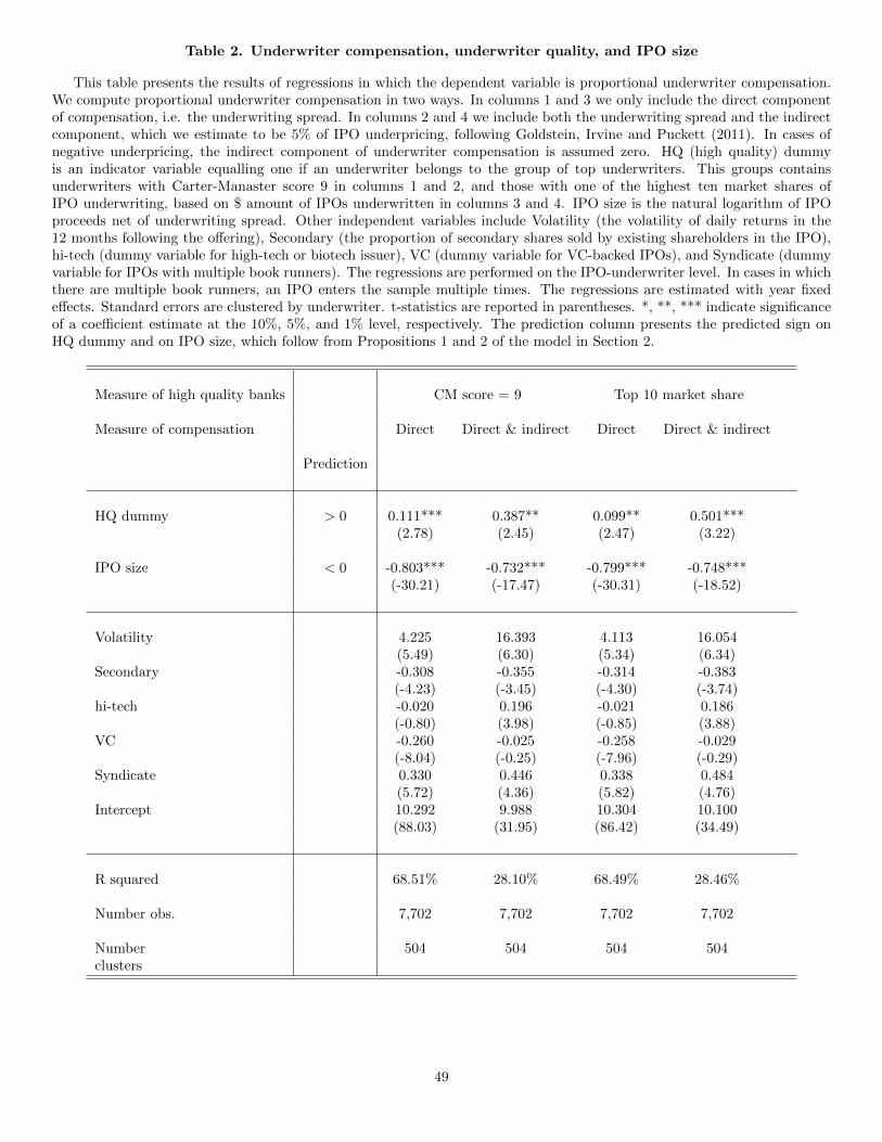
Table 2. Underwriter compensation, underwriter quality, and IPO size

This table presents the results of regressions in which the dependent variable is proportional underwriter compensation.We compute proportional underwriter compensation in two ways. In columns 1 and 3 we only include the direct componentof compensation, i.e. the underwriting spread. In columns 2 and 4 we include both the underwriting spread and the indirectcomponent, which we estimate to be 5% of IPO underpricing, following Goldstein, Irvine and Puckett (2011). In cases ofnegative underpricing, the indirect component of underwriter compensation is assumed zero. HQ (high quality) dummyis an indicator variable equalling one if an underwriter belongs to the group of top underwriters. This groups containsunderwriters with Carter-Manaster score 9 in columns 1 and 2, and those with one of the highest ten market shares ofIPO underwriting, based on $ amount of IPOs underwritten in columns 3 and 4. IPO size is the natural logarithm of IPOproceeds net of underwriting spread. Other independent variables include Volatility (the volatility of daily returns in the12 months following the o↵ering), Secondary (the proportion of secondary shares sold by existing shareholders in the IPO),hi-tech (dummy variable for high-tech or biotech issuer), VC (dummy variable for VC-backed IPOs), and Syndicate (dummyvariable for IPOs with multiple book runners). The regressions are performed on the IPO-underwriter level. In cases in whichthere are multiple book runners, an IPO enters the sample multiple times. The regressions are estimated with year fixede↵ects. Standard errors are clustered by underwriter. t-statistics are reported in parentheses. *, **, *** indicate significanceof a coe�cient estimate at the 10%, 5%, and 1% level, respectively. The prediction column presents the predicted sign onHQ dummy and on IPO size, which follow from Propositions 1 and 2 of the model in Section 2.

Measure of high quality banks CM score = 9 Top 10 market share

Measure of compensation Direct Direct & indirect Direct Direct & indirect

Prediction

HQ dummy > 0 0.111*** 0.387** 0.099** 0.501***(2.78) (2.45) (2.47) (3.22)

IPO size < 0 -0.803*** -0.732*** -0.799*** -0.748***(-30.21) (-17.47) (-30.31) (-18.52)

Volatility 4.225 16.393 4.113 16.054(5.49) (6.30) (5.34) (6.34)

Secondary -0.308 -0.355 -0.314 -0.383(-4.23) (-3.45) (-4.30) (-3.74)

hi-tech -0.020 0.196 -0.021 0.186(-0.80) (3.98) (-0.85) (3.88)

VC -0.260 -0.025 -0.258 -0.029(-8.04) (-0.25) (-7.96) (-0.29)

Syndicate 0.330 0.446 0.338 0.484(5.72) (4.36) (5.82) (4.76)

Intercept 10.292 9.988 10.304 10.100(88.03) (31.95) (86.42) (34.49)

R squared 68.51% 28.10% 68.49% 28.46%

Number obs. 7,702 7,702 7,702 7,702

Number 504 504 504 504clusters

49

Table

3.Under

writerco

mpen

sation,under

writerquality,and

thestate

ofth

eIP

Omark

et

This

table

presentstheresultsof

regression

sin

whichthedep

endentvariab

leis

meanan

nual

proportion

alunderwritercompensation

.Wecompute

propor-

tion

alunderwritercompensation

intw

oways.

Inod

dcolumnsweon

lyincludethedirectcompon

entof

compensation

,i.e.

theunderwritingspread

.In

even

columnsweincludeboththeunderwritingspread

andtheindirectcompon

ent,whichweestimateto

be5%

ofIP

Ounderpricing,

follow

ingGoldstein,Irvinean

dPuckett(2011).In

casesof

negativeunderpricing,

theindirectcompon

entof

underwritercompensation

isassumed

zero.Themaindep

endentvariab

lesarethe

stateof

theIP

Omarket(IPO

state)

interacted

withhighqu

alityan

dlow

qualityunderwriterindicators(H

Qan

dLQ

respectively),

andthestateof

theIP

Omarketsquared.Weuse

threemeasuresof

thestateof

theIP

Omarket.

Thefirston

e,usedin

columns1-4,

isthean

nual

number

ofIP

Os,divided

by100.

The

secondon

e,usedin

columns5-8,

isthean

nual

grow

thin

private

non

residential

fixedinvestment.

Thethirdon

e,usedin

columns9-12,is

thevalue-weigh

ted

annu

almarketreturn.HQ

(highqu

ality)

dummyisan

indicator

variab

leequallingon

eifan

underwriterbelon

gsto

thegrou

pof

topunderwriters.Thisgrou

ps

containsunderwriters

withCarter-Man

asterscore9in

columns1,

2,5,

6,9,

and10,an

dthosewithon

eof

thehighesttenmarketshares

ofIP

Ounderwriting,

based

on$am

ount

ofIP

Osunderwritten,in

columns3,

4,7,

8,11,an

d12.IP

OSizeis

thenaturallogarithm

ofIP

Oproceedsnet

ofunderwritingspread

.Other

indep

endentvariab

lesincludeVolatility(m

eanvolatility

ofdaily

returnsin

the12

mon

thsfollow

ingtheo↵

erings

byagivenunderwriterin

agivenyear),

Secon

dary(m

eanproportion

ofsecondaryshares

sold

byexistingshareholdersin

IPOsby

agivenunderwriterin

agivenyear),hi-tech

(proportion

ofhigh-tech

orbiotech

issuers),VC

(proportion

ofVC-backedIP

Os),an

dSyn

dicate(proportion

ofIP

Oswithjointboo

krunners).Theregression

sareperform

edat

the

underwriter-year

level.

Standarderrors

areclustered

byunderwriter.

t-statistics

arereportedin

parentheses.*,

**,***indicatesign

ificance

ofacoe�

cient

estimateat

the10%,5%

,an

d1%

level,respectively.Theprediction

columnpresentsthepredictedsign

onIP

Ostate*HQ,IP

Ostate*LQ,an

dIP

Ostate2,

whichfollow

from

Proposition3of

themod

elin

Section

2.

50

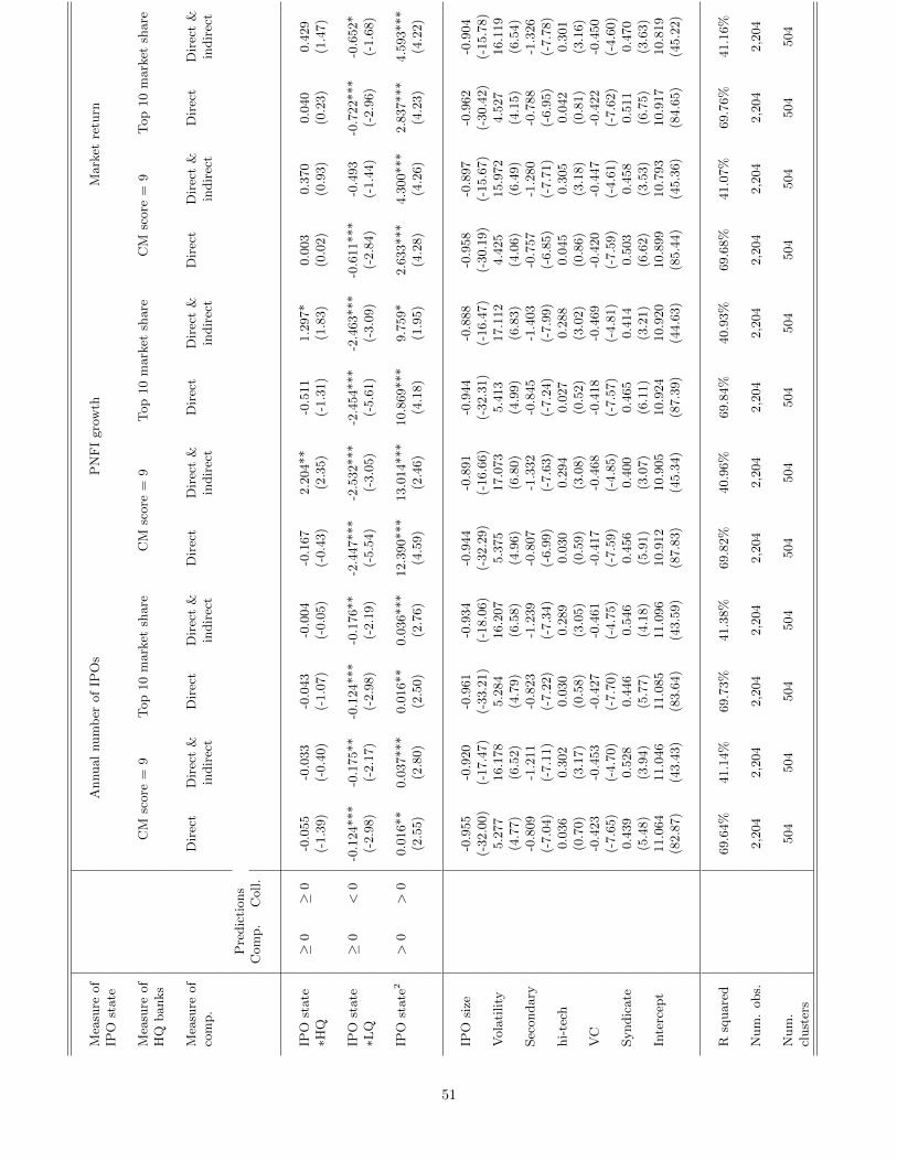
Measure

ofAnnual

number

ofIP

Os

PNFIgrow

thMarketreturn

IPO

state

Measure

ofCM

score=

9Top

10marketshare

CM

score=

9Top

10marketshare

CM

score=

9Top

10marketshare

HQ

ban

ks

Measure

ofDirect

Direct&

Direct

Direct&

Direct

Direct&

Direct

Direct&

Direct

Direct&

Direct

Direct&

comp.

indirect

indirect

indirect

indirect

indirect

indirect

Prediction

sCom

p.

Coll.

IPO

state

�0

�0

-0.055

-0.033

-0.043

-0.004

-0.167

2.20

4**

-0.511

1.29

7*0.00

30.37

00.04

00.42

9⇤H

Q(-1.39

)(-0.40

)(-1.07

)(-0.05

)(-0.43

)(2.35)

(-1.31

)(1.83)

(0.02)

(0.93)

(0.23)

(1.47)

IPO

state

�0

<0

-0.124

***

-0.175

**-0.124

***

-0.176

**-2.447

***

-2.532

***

-2.454

***

-2.463

***

-0.611

***

-0.493

-0.722

***

-0.652

*⇤L

Q(-2.98

)(-2.17

)(-2.98

)(-2.19

)(-5.54

)(-3.05

)(-5.61

)(-3.09

)(-2.84

)(-1.44

)(-2.96

)(-1.68

)

IPO

state2

>0

>0

0.01

6**

0.03

7***

0.01

6**

0.03

6***

12.390

***

13.014

***

10.869

***

9.75

9*2.63

3***

4.30

0***

2.83

7***

4.59

3***

(2.55)

(2.80)

(2.50)

(2.76)

(4.59)

(2.46)

(4.18)

(1.95)

(4.28)

(4.26)

(4.23)

(4.22)

IPO

size

-0.955

-0.920

-0.961

-0.934

-0.944

-0.891

-0.944

-0.888

-0.958

-0.897

-0.962

-0.904

(-32

.00)

(-17

.47)

(-33

.21)

(-18

.06)

(-32

.29)

(-16

.66)

(-32

.31)

(-16

.47)

(-30

.19)

(-15

.67)

(-30

.42)

(-15

.78)

Volatility

5.27

716

.178

5.28

416

.207

5.37

517

.073

5.41

317

.112

4.42

515

.972

4.52

716

.119

(4.77)

(6.52)

(4.79)

(6.58)

(4.96)

(6.80)

(4.99)

(6.83)

(4.06)

(6.49)

(4.15)

(6.54)

Secon

dary

-0.809

-1.211

-0.823

-1.239

-0.807

-1.332

-0.845

-1.403

-0.757

-1.280

-0.788

-1.326

(-7.04

)(-7.11

)(-7.22

)(-7.34

)(-6.99

)(-7.63

)(-7.24

)(-7.99

)(-6.85

)(-7.71

)(-6.95

)(-7.78

)hi-tech

0.03

60.30

20.03

00.28

90.03

00.29

40.02

70.28

80.04

50.30

50.04

20.30

1(0.70)

(3.17)

(0.58)

(3.05)

(0.59)

(3.08)

(0.52)

(3.02)

(0.86)

(3.18)

(0.81)

(3.16)

VC

-0.423

-0.453

-0.427

-0.461

-0.417

-0.468

-0.418

-0.469

-0.420

-0.447

-0.422

-0.450

(-7.65

)(-4.70

)(-7.70

)(-4.75

)(-7.59

)(-4.85

)(-7.57

)(-4.81

)(-7.59

)(-4.61

)(-7.62

)(-4.60

)Syndicate

0.43

90.52

80.44

60.54

60.45

60.40

00.46

50.41

40.50

30.45

80.51

10.47

0(5.48)

(3.94)

(5.77)

(4.18)

(5.91)

(3.07)

(6.11)

(3.21)

(6.62)

(3.53)

(6.75)

(3.63)

Intercep

t11

.064

11.046

11.085

11.096

10.912

10.905

10.924

10.920

10.899

10.793

10.917

10.819

(82.87

)(43.43

)(83.64

)(43.59

)(87.83

)(45.34

)(87.39

)(44.63

)(85.44

)(45.36

)(84.65

)(45.22

)

Rsquared

69.64%

41.14%

69.73%

41.38%

69.82%

40.96%

69.84%

40.93%

69.68%

41.07%

69.76%

41.16%

Num.ob

s.2,20

42,20

42,20

42,20

42,20

42,20

42,20

42,20

42,20

42,20

42,20

42,20

4

Num.

504

504

504

504

504

504

504

504

504

504

504

504

clusters

51

Table

4.Ratioofhigh-quality

tolow-quality

under

writerco

mpen

sation

and

thestate

ofth

eIP

Omark

et

This

table

presentstheresultsof

regression

sin

which

thedep

endentvariab

leis

thenaturallogarithm

oftheratioof

annu

almean

absolute

(dollar)

compensation

ofan

underwriterthat

belon

gsto

ahighqu

alitygrou

pto

annu

almeanab

solute

(dollar)

compensation

ofunderwriters

that

donot

belon

gto

ahighqu

alitygrou

p.Wecompute

absolute

(dollar)

underwritercompensation

intw

oway

s.In

oddcolumnsweon

lyincludethedirectcompon

entof

the

compensation

,i.e.

theunderwritingspread

multiplied

byissueproceeds.

Ineven

columnsweincludeboththeunderwritingspread

multiplied

byissueproceeds

andtheindirectcompon

ent,

whichweestimateto

be5%

ofIP

Ounderpricingmultiplied

byissueproceeds.

Incasesof

negativeunderpricing,

theindirect

compon

entof

underwritercompensation

isassumed

zero.Themaindep

endentvariab

lesarethestateof

theIP

Omarket(IPO

state)

andthestateof

theIP

Omarketsquared.Weuse

threemeasuresof

thestateof

theIP

Omarket.

Thefirston

e,usedin

columns1-4,

isthean

nual

number

ofIP

Os,divided

by100.

The

secondon

e,usedin

columns5-8,

isthean

nual

grow

thin

private

non

residential

fixedinvestment.

Thethirdon

e,usedin

columns9-12,is

thevalue-weigh

ted

annu

almarketreturn.Thegrou

pof

highqu

alityunderwriters

containsunderwriters

withCarter-Man

asterscore9in

columns1,

2,5,

6,9,

and10,an

dthose

withthehighesttenmarketshares

ofIP

Ounderwriting,

based

on$am

ount

ofIP

Osunderwritten,in

columns3,

4,7,

8,11,an

d12.Di↵

variab

lesrefer

tothedi↵erence

betweenan

nual

meanof

thevariab

leforahighqu

alityunderwriteran

dan

nual

meanvalueof

thevariab

lewithin

thegrou

pof

low

quality

underwriters.IP

OSizeis

thenaturallogarithm

ofIP

Oproceedsnet

ofunderwritingspread

.Other

indep

endentvariab

lesincludeVolatility(m

eanvolatility

ofdaily

returnsin

the12

mon

thsfollow

ingtheo↵

erings

byagivenunderwriterin

agivenyear),

Secon

dary(m

eanproportion

ofsecondaryshares

sold

byexistingshareholdersin

theIP

Oby

agivenunderwriterin

agivenyear),

hi-tech

(proportion

ofhigh-techor

biotech

issuers),VC

(proportion

ofVC-backed

IPOs),an

dSyn

dicate(proportion

ofIP

Oswithmultiple

boo

krunners).Theregression

sareperform

edat

theunderwriter-year

levelforsamplesof

highqu

ality

underwriters.Standarderrors

areclustered

byunderwriter.

t-statistics

arereportedin

parentheses.*,

**,***indicatesign

ificance

ofacoe�

cientestimateat

the10%,5%

,an

d1%

level,respectively.Theprediction

columnpresentsthepredictedsign

onIP

Ostatean

dIP

Ostate2,whichfollow

from

Proposition4of

themod

elin

Section

2.

52

Measure

ofAnnual

number

ofIP

Os

PNFIgrow

thMarketreturn

IPO

state

Measure

ofCM

score=

9Top

10marketshare

CM

score=

9Top

10marketshare

CM

score=

9Top

10marketshare

HQ

ban

ks

Measure

ofDirect

Direct&

Direct

Direct&

Direct

Direct&

Direct

Direct&

Direct

Direct&

Direct

Direct&

comp.

indirect

indirect

indirect

indirect

indirect

indirect

Prediction

sCom

p.

Coll.

IPO

state

<=

0>

00.04

2*0.04

6*0.11

2***

0.10

0***

0.29

50.34

50.08

50.07

70.21

3**

0.27

1***

0.17

70.12

5(1.70)

(1.72)

(5.69)

(5.17)

(1.30)

(1.53)

(0.50)

(0.44)

(2.38)

(3.70)

(1.48)

(1.07)

IPO

state2

<0

<0

-0.001

-0.002

-0.015

***

-0.012

***

-5.189

***

-6.121

***

-3.566

***

-3.594

***

-0.414

-0.455

-0.883

**-0.471

(-0.21

)(-0.35

)(-5.15

)(-3.99

)(-3.38

)(-3.58

)(-3.57

)(-3.24

)(-1.03

)(-1.12

)(-2.03

)(-1.08

)

Di↵

IPO

size

0.90

30.89

50.79

40.80

50.91

40.90

80.78

40.79

50.90

10.89

20.80

30.80

8(32.96

)(33.41

)(14.86

)(16.83

)(33.95

)(34.53

)(14.22

)(16.18

)(34.09

)(33.93

)(15.95

)(17.63

)Di↵

volatility

-4.021

-3.495

-0.890

-0.915

-5.775

-5.273

-0.959

-1.128

-6.132

-5.752

0.00

6-0.376

(-2.00

)(-1.38

)(-0.66

)(-0.75

)(-3.52

)(-2.43

)(-0.86

)(-1.14

)(-3.74

)(-2.69

)(0.00)

(-0.33

)Di↵

secondary

-0.132

-0.132

0.06

8-0.031

-0.190

-0.193

0.03

4-0.063

-0.181

-0.183

-0.040

-0.125

(-1.77

)(-1.56

)(0.63)

(-0.29

)(-2.61

)(-2.26

)(0.31)

(-0.57

)(-2.23

)(-1.92

)(-0.42

)(-1.28

)Di↵

hi-tech

0.04

70.05

6-0.026

0.00

80.08

50.09

9-0.039

-0.004

0.06

20.07

30.00

00.02

4(0.96)

(1.04)

(-0.61

)(0.18)

(1.56)

(1.60)

(-0.91

)(-0.09

)(1.24)

(1.33)

(0.01)

(0.55)

Di↵

VC

-0.033

0.00

00.00

40.03

5-0.051

-0.020

0.02

30.05

7-0.044

-0.012

-0.035

0.01

0(-0.80

)(0.00)

(0.08)

(0.78)

(-1.10

)(-0.41

)(0.43)

(1.11)

(-0.97

)(-0.26

)(-0.70

)(0.20)

Di↵

-0.757

-0.787

-0.819

-0.734

-0.813

-0.839

-0.929

-0.846

-0.814

-0.838

-0.844

-0.779

syndicate

(-5.44

)(-5.47

)(-9.92

)(-9.02

)(-6.73

)(-6.75

)(-10

.01)

(-9.34

)(-6.36

)(-6.16

)(-9.14

)(-8.21

)Intercep

t-0.249

-0.239

-0.126

-0.113

-0.201

-0.192

0.04

40.05

0-0.183

-0.176

0.02

30.02

1(-9.96

)(-8.75

)(-2.49

)(-2.48

)(-6.94

)(-6.23

)(0.73)

(0.93)

(-5.10

)(-4.54

)(0.41)

(0.41)

Rsquared

89.68%

87.10%

86.66%

86.48%

89.32%

86.86%

85.84%

85.69%

89.20%

86.74%

85.76%

85.41%

Num.ob

s.32

332

337

837

832

332

337

837

832

332

337

837

8

Num.

3131

5757

3131

5757

3131

5757

clusters

53

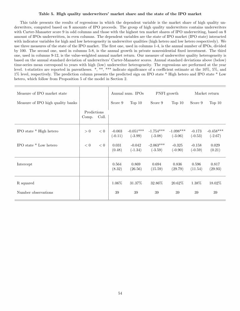
Table 5. High quality underwriters’ market share and the state of the IPO market

This table presents the results of regressions in which the dependent variable is the market share of high quality un-derwriters, computed based on $ amounts of IPO proceeds. The group of high quality underwriters contains underwriterswith Carter-Manaster score 9 in odd columns and those with the highest ten market shares of IPO underwriting, based on $amount of IPOs underwritten, in even columns. The dependent variables are the state of IPO market (IPO state) interactedwith indicator variables for high and low heterogeneity in underwriter qualities (high hetero and low hetero respectively). Weuse three measures of the state of the IPO market. The first one, used in columns 1-4, is the annual number of IPOs, dividedby 100. The second one, used in columns 5-8, is the annual growth in private nonresidential fixed investment. The thirdone, used in columns 9-12, is the value-weighted annual market return. Our measure of underwriter quality heterogeneity isbased on the annual standard deviation of underwriters’ Carter-Manaster scores. Annual standard deviations above (below)time-series mean correspond to years with high (low) underwriter heterogeneity. The regressions are performed at the yearlevel. t-statistics are reported in parentheses. *, **, *** indicate significance of a coe�cient estimate at the 10%, 5%, and1% level, respectively. The prediction column presents the predicted sign on IPO state * High hetero and IPO state * Lowhetero, which follow from Proposition 5 of the model in Section 2.

Measure of IPO market state Annual num. IPOs PNFI growth Market return

Measure of IPO high quality banks Score 9 Top 10 Score 9 Top 10 Score 9 Top 10

PredictionsComp. Coll.

IPO state * High hetero > 0 < 0 -0.003 -0.051*** -1.754*** -1.098*** -0.173 -0.458***(-0.11) (-3.99) (-3.08) (-3.06) (-0.53) (-2.67)

IPO state * Low hetero < 0 < 0 0.031 -0.042 -2.063*** -0.325 -0.158 0.029(0.48) (-1.34) (-3.59) (-0.90) (-0.59) (0.21)

Intercept 0.564 0.869 0.694 0.836 0.596 0.817(8.32) (26.56) (15.59) (29.79) (11.54) (29.93)

R squared 1.06% 31.37% 32.86% 20.62% 1.38% 18.02%

Number observations 39 39 39 39 39 39

54

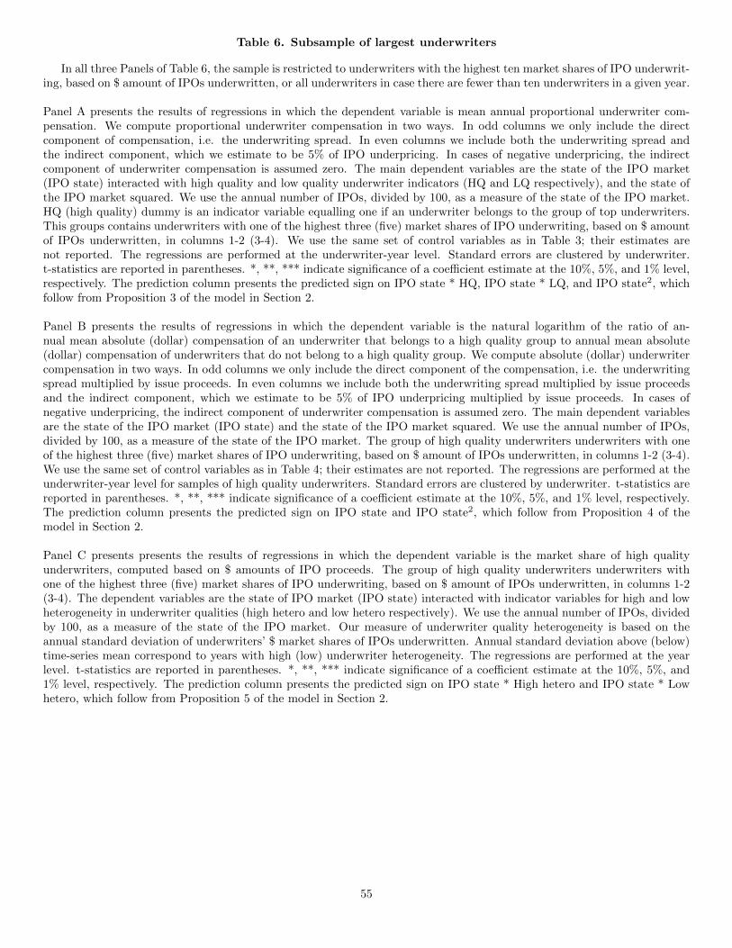
Table 6. Subsample of largest underwriters

In all three Panels of Table 6, the sample is restricted to underwriters with the highest ten market shares of IPO underwrit-ing, based on $ amount of IPOs underwritten, or all underwriters in case there are fewer than ten underwriters in a given year.

Panel A presents the results of regressions in which the dependent variable is mean annual proportional underwriter com-pensation. We compute proportional underwriter compensation in two ways. In odd columns we only include the directcomponent of compensation, i.e. the underwriting spread. In even columns we include both the underwriting spread andthe indirect component, which we estimate to be 5% of IPO underpricing. In cases of negative underpricing, the indirectcomponent of underwriter compensation is assumed zero. The main dependent variables are the state of the IPO market(IPO state) interacted with high quality and low quality underwriter indicators (HQ and LQ respectively), and the state ofthe IPO market squared. We use the annual number of IPOs, divided by 100, as a measure of the state of the IPO market.HQ (high quality) dummy is an indicator variable equalling one if an underwriter belongs to the group of top underwriters.This groups contains underwriters with one of the highest three (five) market shares of IPO underwriting, based on $ amountof IPOs underwritten, in columns 1-2 (3-4). We use the same set of control variables as in Table 3; their estimates arenot reported. The regressions are performed at the underwriter-year level. Standard errors are clustered by underwriter.t-statistics are reported in parentheses. *, **, *** indicate significance of a coe�cient estimate at the 10%, 5%, and 1% level,respectively. The prediction column presents the predicted sign on IPO state * HQ, IPO state * LQ, and IPO state2, whichfollow from Proposition 3 of the model in Section 2.

Panel B presents the results of regressions in which the dependent variable is the natural logarithm of the ratio of an-nual mean absolute (dollar) compensation of an underwriter that belongs to a high quality group to annual mean absolute(dollar) compensation of underwriters that do not belong to a high quality group. We compute absolute (dollar) underwritercompensation in two ways. In odd columns we only include the direct component of the compensation, i.e. the underwritingspread multiplied by issue proceeds. In even columns we include both the underwriting spread multiplied by issue proceedsand the indirect component, which we estimate to be 5% of IPO underpricing multiplied by issue proceeds. In cases ofnegative underpricing, the indirect component of underwriter compensation is assumed zero. The main dependent variablesare the state of the IPO market (IPO state) and the state of the IPO market squared. We use the annual number of IPOs,divided by 100, as a measure of the state of the IPO market. The group of high quality underwriters underwriters with oneof the highest three (five) market shares of IPO underwriting, based on $ amount of IPOs underwritten, in columns 1-2 (3-4).We use the same set of control variables as in Table 4; their estimates are not reported. The regressions are performed at theunderwriter-year level for samples of high quality underwriters. Standard errors are clustered by underwriter. t-statistics arereported in parentheses. *, **, *** indicate significance of a coe�cient estimate at the 10%, 5%, and 1% level, respectively.The prediction column presents the predicted sign on IPO state and IPO state2, which follow from Proposition 4 of themodel in Section 2.

Panel C presents presents the results of regressions in which the dependent variable is the market share of high qualityunderwriters, computed based on $ amounts of IPO proceeds. The group of high quality underwriters underwriters withone of the highest three (five) market shares of IPO underwriting, based on $ amount of IPOs underwritten, in columns 1-2(3-4). The dependent variables are the state of IPO market (IPO state) interacted with indicator variables for high and lowheterogeneity in underwriter qualities (high hetero and low hetero respectively). We use the annual number of IPOs, dividedby 100, as a measure of the state of the IPO market. Our measure of underwriter quality heterogeneity is based on theannual standard deviation of underwriters’ $ market shares of IPOs underwritten. Annual standard deviation above (below)time-series mean correspond to years with high (low) underwriter heterogeneity. The regressions are performed at the yearlevel. t-statistics are reported in parentheses. *, **, *** indicate significance of a coe�cient estimate at the 10%, 5%, and1% level, respectively. The prediction column presents the predicted sign on IPO state * High hetero and IPO state * Lowhetero, which follow from Proposition 5 of the model in Section 2.

55

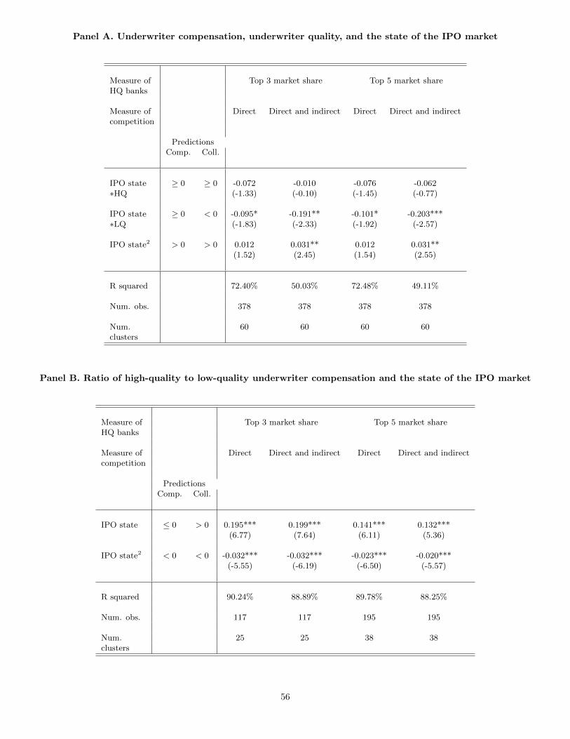
Panel A. Underwriter compensation, underwriter quality, and the state of the IPO market

Measure of Top 3 market share Top 5 market shareHQ banks

Measure of Direct Direct and indirect Direct Direct and indirectcompetition

PredictionsComp. Coll.

IPO state � 0 � 0 -0.072 -0.010 -0.076 -0.062⇤HQ (-1.33) (-0.10) (-1.45) (-0.77)

IPO state � 0 < 0 -0.095* -0.191** -0.101* -0.203***⇤LQ (-1.83) (-2.33) (-1.92) (-2.57)

IPO state2 > 0 > 0 0.012 0.031** 0.012 0.031**(1.52) (2.45) (1.54) (2.55)

R squared 72.40% 50.03% 72.48% 49.11%

Num. obs. 378 378 378 378

Num. 60 60 60 60clusters

Panel B. Ratio of high-quality to low-quality underwriter compensation and the state of the IPO market

Measure of Top 3 market share Top 5 market shareHQ banks

Measure of Direct Direct and indirect Direct Direct and indirectcompetition

PredictionsComp. Coll.

IPO state 0 > 0 0.195*** 0.199*** 0.141*** 0.132***(6.77) (7.64) (6.11) (5.36)

IPO state2 < 0 < 0 -0.032*** -0.032*** -0.023*** -0.020***(-5.55) (-6.19) (-6.50) (-5.57)

R squared 90.24% 88.89% 89.78% 88.25%

Num. obs. 117 117 195 195

Num. 25 25 38 38clusters

56

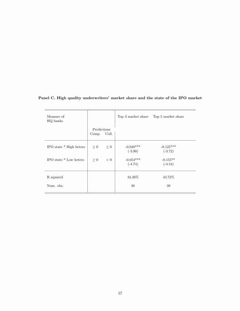
Panel C. High quality underwriters’ market share and the state of the IPO market

Measure of Top 3 market share Top 5 market shareHQ banks

PredictionsComp. Coll.

IPO state * High hetero � 0 � 0 -0.048*** -0.125***(-3.90) (-3.72)

IPO state * Low hetero � 0 < 0 -0.054*** -0.155**(-4.74) (-4.54)

R squared 34.38% 43.72%

Num. obs. 39 39

57