Do individuals recognize cascade behavior ofothers?

– An experimental study –∗

Andreas StiehlerMax Planck Institute

for Research into Economic SystemsStrategic Interaction GroupKahlaische Straße 10

D - 07745 Jena, Germanystiehler@mpiew-jena.mpg.de

AbstractIn a cascade experiment subjects are confronted with artificial prede-

cessors predicting in line with the BHW model (Bikhchandani, Hirshleiferand Welch, 1992). Using the BDM mechanism we study subjects’ proba-bility assignments based on price limits for participating in the predictiongame. We find increasing price limits the more coinciding predictions ofpredecessors are observed and regardless of whether additional informationis actually revealed by predecessors’ predictions. Individual price patternsof more than two thirds of the participants indicate that cascade behaviorof predecessors is not recognized.JEL Classification: C91, D81, D82Key Words: information cascades, Bayes’ rule, decisions under risk and

uncertainty, experimental economics

∗I especially thank Tim Grebe who did the programming and assisted when running theexperiments. Moreover, I thank Sabine Kröger, Sveta Ivanova-Stenzel, Anthony Ziegelmeyer,Clemens Oberhammer, Werner Güth and the participants of the summerschool workshop (2002)at Max Planck Institute Jena for their helpful comments. The financial support by DeutscheForschungsgemeinschaft (DFG 373) is gratefully acknowledged.

1. Introduction

Information cascades as modelled by Bikhchandani, Hirshleifer and Welch (1992),

henceforth BHW, have become a very popular approach to explain herding be-

havior, especially among economists.1 The BHW model can be used to explain

central features of herding as erroneous mass behavior and can account for many

examples to be found in practice. But herding can also be derived within a ratio-

nal choice approach assuming agents who update information according to Bayes’

rule. Last but not least, the BHW model also withstood a first experimental test

by Anderson and Holt (1997), henceforth AH.2 It shows that in a choice situation

under incomplete private information it may be rational just to follow predecessors

by disregarding one’s own private information. Hence a cascade starts since no

further information will be aggregated. Agents may follow wrong decisions of pre-

decessors even if the aggregated private information would suggest the opposite.

Individual rationality may thus lead to market inefficiencies.

The BHW model implicitly assumes that agents recognize cascade behavior

of others. If not, perceived posterior probabilities increase with the length of the

cascade even if no further information aggregation takes place. Boundedly rational

behavior of agents thus would result in an overvaluation of public information and

thereby cause economic consequences. Consumers, for instance, might misinter-

pret past sales of a specific product as signaling quality. They consequently may

be willing to pay unreasonably high prices for best-sellers compared to competing

products with similar features. Promotion instruments, that refer to number or

1For an online survey of theoretical and empirical studies faced with information cascades seeBikhchandy, Hirshleifer and Welch (1996) available at [http://welch.som.yale.edu/cascades/].

2They ran a prediction game in which the underlying information structure of BHW wasreflected by urns and balls and conclusions drawn from subjects’ urn predictions.

degree of already made sales as, e.g. best-seller lists, could not only be used to

raise sales numbers but also to get consumers to accept price increases.3

Whether individuals actually recognize cascade behavior of others is the fo-

cus of this study. The answer to this question is not only of practical relevance

as discussed above; it is also of theoretical interest. Following AH, most previous

experimental studies investigate cascade behavior by varying the underlying infor-

mation structure and selling costly private information.4 Conclusions are usually

drawn from subjects’ predictions and buying decisions. It turned out that individ-

uals, if confronted with more complex decision tasks, tend to overestimate private

information and thus to deviate from the rational cascade pattern. They follow

their private signal longer than predicted by BHW and buy more information than

would be rational. Even in the AH experiment itself prediction errors increase up

to 50 percent if simple counting does not lead to a correct urn prediction (see

Huck and Oechsler, 2000). In these situations the rule ‘follow your own signal’

offers better predictions than Bayesian updating.

In contrast, we especially focus on individual updating behavior if confronted

with a symmetric cascade design, in which even simple counting inherently leads to

correct urn predictions. We conjecture that people confronted with these rather

simple decision tasks predict according to theory but do not recognize cascade

behavior of others and, hence, tend to overestimate public information.

Oberhammer and Stiehler (2002) already investigated whether cascade be-

havior in a symmetric cascade design reflects Bayesian updating. Using the BDM

procedure (Becker, De Groot and Marshak, 1964) they asked participants to sub-

mit maximum prices they are willing to pay to participate in the prediction game.

This enables them to use maximum prices as indicators of subjective probabil-

ity perceptions and thus to test directly the explanatory power of the standard

BHW model as well as of cascade models in which errors of predecessors are in-

cluded in subjects’ updating process.5 The authors report on increasing prices3We are aware, that in markets in which prices instantly and smoothly adjust, as e.g. in

financial markets, prices would incorporate additional public information and thus rule out in-formation cascades as shown by Avery and Zemsky (1998) and experimentally tested by Ciprianiand Guarino (2001) and Drehmann at al.(2002).

4See e.g.Willinger and Ziegelmeyer (1998), Kraemer at al. (2000), Kraemer and Weber(2001), Nöth and Weber (2001), Kübler and Weizsäcker (2001).

5The examination of errors by econometric methods in so called quantal response models(McKelvey and Palfrey 1995,1998) has become increasingly popular for the analysis of cascadedata, since resulting approaches inter alia can account for a significant portion of deviationsfrom standard BHW model as reported above. For different approaches of quantal responseequilibria in information cascade models see e.g. Anderson and Holt (1997), Anderson (2001),Kübler and Weizsäcker (forthcoming) or Kreamer and Noeth (2001).

2

up to cascade positions at which no further information is revealed by predic-

tions of predecessors. In contrast to the standard BHW model, error models can

account for the observed price increase. But the observed pattern could also be

caused by subjects who do not recognize cascade behavior of others and, thus,

overestimate public information. Even if the authors succeeded in designing an

experiment that provides more insight into subjects’ updating behavior, they were

not able yet to distinguish between different explanations for the observed price

setting pattern. Moreover, their data source is limited. The cascade situations in

which individuals have to decide are endogenously determined, so that observing

complete individual price patterns is nearly impossible.

In this experiment we use a similar design as Oberhammer and Stiehler

(2002). Subjects are confronted with the same information structure and the

BDM mechanism is used to extract prices as indicators of subjects’ probability

perceptions. In addition, artificial agents are incorporated as predecessors, who

follow a simple counting rule and - by definition - never err. Using a strategy

method subjects are asked to state their decisions for all possible cascade situ-

ations. Clearly such a design allows to address the central question of whether

individuals recognize cascade behavior of others on the basis of complete individ-

ual price setting patterns with individual price decisions for all possible cascade

positions.

The remainder of this paper is organized as follows: In section 2 the experi-

mental design and procedures are described. In the subsequent section 3 predic-

tions are derived for both rational behavior as assumed in the BHW model and

behavior based on the assumption that subjects do not recognize cascade behav-

ior of others. The results are presented in section 4. The paper finishes with a

discussion of the results in section 5.

2. Experimental design and procedure

We incorporate artificial agents and apply the strategy method in a design similar

to Oberhammer and Stiehler (2002). One of our major concerns when planning

the procedure was to ensure that all design features were clearly understood by

the participants. In this section each part of the design and the experimental

procedure will be explained in detail and discussed in the light of our central

question to be tested.

3

Experimental scenario

There are two urns, A and B, with 5 balls each (3 white balls and 2 black

balls and vice versa). One urn is randomly chosen with equal probability at the

beginning, and players predict repeatedly the randomly chosen urn. For a correct

urn prediction they receive 100 ECU (Experimental Currency Units) and nothing

else. As participant’s private information a ball is drawn from the urn and its

color revealed. As public information predecessors’ urn predictions are publicly

announced.

Participants are further asked to submit maximum prices pmax they are willing

to pay to participate in the prediction game, i.e. to seize the chance of winning

100 ECU for a correct urn prediction. As an incentive compatible mechanism to

elicit subjects’ maximum willingness to pay we implemented the Becker-DeGroot-

Marshak (BDM) mechanism (Becker, DeGroot and Marshak, 1964). A uniformly

distributed random price pr from the interval [0,100] is drawn and compared with

the maximum prices submitted by the participants. If the random price exceeds

the maximum price (pr > pmax) the participant earns nothing. If the random

price is equal or lower than the maximum price (pr ≤ pmax) the participant earnsthe money amount resulting from her urn prediction minus the random price (see

also Table 2.1).

Correct urn prediction Wrong urn predictionpr ≤ pmax 100 ECU - pr 0 ECU - prpr > pmax 0 ECU 0 ECU

Table 2.1: Income calculation.

If participants were risk neutral and would maximize their income according

to standard expected utility theory the submitted maximum prices would perfectly

reflect their probability perceptions. But these assumptions are hardly satisfied

as many experimental studies on decision making show.6 We are also aware that

the implementation of the BDM mechanism in a lottery-like decision task might

provoke preference reversals (Safra et al., 1990).

However, for our purpose it is sufficient if prices and probabilities are posi-

tively correlated. Under the assumption of a positive correlation we are able to

6For surveys of experimental studies on individual decision making under risk and uncertaintysee e.g. Camerer (1995) or Hey (1991).

4

compare resulting price patterns with the probability pattern according to BHW.

To test this necessary assumption participants are additionally asked to state sub-

jective probabilities for the correctness of their urn predictions. For 38 out of 39

participants (97.4 %) we observe highly significant positive correlations between

maximum prices and subjective probabilities and thus consider this assumption

as fulfilled.

Implementation of artificial agents

In this cascade experiment a subject’s predecessors are artificial agents, whose

predictions are clearly defined by simple counting, e.g. agents predict according to

the majority of (public and private) signals in favor of Urn A or B. Consequently,

errors of predecessors are excluded by definition. Note that in the applied sym-

metrical information structure simple counting leads to the same urn predictions

as Bayesian updating (see Anderson and Holt, 1997). Thus urn predictions of

predecessors are in line with BHW. In case of a tie-break, i.e. an equal number

of signals in favor of urn A and B, artificial agents decide according to their pri-

vate signal. This tie-breaking rule, that was also assumed by AH to analyze data

of the symmetric design, rather simplifies the updating process compared to a

randomization between urn A and B, as assumed by BHW.

One may object that we influenced participants’ decisions by incorporating

artificial agents who followed a simple counting heuristic. That might be true since

we, admittedly, teach participants to predict according to the BHW model. But

note that we are interested in price setting behavior rather than in urn predictions.

If maximum prices were also influenced, this would strengthen the evidence against

the hypothesis, that subjects do not recognize cascade behavior of others. We,

however, find this hypothesis supported by the data as will be reported in section

4.

Use of the strategy method

Participants are asked to state their decisions for all resulting situations up to

position 6 (and thus are confronted with up to 5 artificial agents as predecessors).

Depending on

• participants’ own positions (1 to 6),

5

• the color of the privately drawn ball (black or white) and

• the history regarding predecessors’ predictions

there are overall 74 cascade situations (summarized in Appendix C) for which

participants have to submit their urn predictions and their maximum prices. One

situation was randomly chosen at the end of the session to be paid out according to

each participant’s respective decisions and the outcome of the random processes.

The choice of the payment-relevant situation works as follows:

1. One urn (A or B) is randomly chosen.

2. Subjects’ position (1 to 6) is determined.

3. For each artificial agent a ball is drawn from the actually chosen urn and

its predictions with respect to the defined decision rules determined and

publicly announced.

4. At (real) participants’ position a ball is drawn and the color announced.

Then one situation (out of 74) is chosen to become payoff-relevant. Further,

the actually chosen urn is revealed and the random price is drawn from all integers

between 0 and 100. Now the incomes from the experiment can be calculated

according to the rules summarized in Table 2.1.

The implementation of the strategy method has two major advantages: First

it enables us to observe complete individual price patterns as discussed in the

previous section. Secondly, the strategy method, as investigated so far causes

rather ‘cold’, i.e. less emotional responses than spontaneous play and thus helps

us to focus on participants ability to recognize cascade behavior of others.7

Procedure

At the start of a session participants were provided with formal instructions

(see Appendix A) as well as with a supplementary sheet on the working of the

BDMmechanism demonstrating that strategic behavior does not pay (see Appen-

dix B). Upcoming questions were answered privately during the whole experiment.

7For experimental studies on presentation effects see e.g. Brandts and Charness (2000) orSchotter, Weigelt and Wilson (1994).

6

After reading the instructions it was demonstrated how the payment-relevant

situation would be chosen. While all decisions had to be submitted via the com-

puter, the choice of the payment-relevant situation and the draw of the random

price were done by hand using real urns (opaque blue bags), balls (table tennis

balls), dice and chips with numbers from 1 to 100. Participants themselves were

asked to execute the random processes.

Before starting the experiment participants were confronted with a pre-experimental

control questionnaire, in which they were systematically asked about decision rules

of artificial predecessors and the work of the price mechanism (see Appendix D).

We provided an additional payment of C= 5 for subjects who answered all ques-

tions correctly in the first go. Moreover, participants were not allowed to proceed

before all questions were answered correctly.

In the experiment participants submitted their decisions for all 74 situations

which were — in random order — displayed on the computer screen. After the

decisions were taken the payment relevant situation (out of 74) was chosen and

subjects paid according to their respective decisions and the outcomes of the

random processes.

By using of real urns and balls and the execution of random choices by partic-

ipants themselves, by demonstrating the choice of the payment-relevant situation

before a session started and by using a pre-experimental control questionnaire we

ensured that the structure of the experiment, the decision rules of artificial agents

as well as the working of BDM were understood by the participants. In addition,

our findings are controlled for a possible bias resulting from lack of understanding

of the artificial agents’ decision rules (see section 4).

The computerized experiment (using the software toolkit z-Tree, Fischbacher,

1999), was conducted at Humboldt-University in Berlin. We ran 4 sessions with

9, 12, 7 and 11 participants. The 39 subjects, mainly students of the economics

faculty, were randomly recruited from a pool of potential participants. In order

to avoid losses a show-up fee of 100 ECU was paid. The experiment lasted about

80 minutes. 100 ECU corresponded to C= 10. Average earnings amounted to

approximately C= 17 on average.

7

3. Hypotheses

In a symmetric cascade structure in which predecessors update information in line

with Bayes’ rule and predict in case of a 50% chance according to their private

signal posterior probabilities just depend on the number of signals in favor of urn

A and B. For the applied design they can be calculated as follows (see Anderson

and Holt,1997 p.850).

Let n(m) be the number of signals in favor of urn A (B). Then:

Pr(A|n,m) =Pr(n,m|A) Pr(A)

Pr(n,m|A) Pr(A) + Pr(n,m|B) Pr(B) (3.1)

=

(35

)n (25

)m (12

)(35

)n (25

)m (12

)+(25

)n (35

)m (12

) (3.2)

It can, furthermore, be shown that under the described assumptions only the

difference between A-and B-signals d = n − m is relevant as illustrated in the

following equation 3.3. If n is substituted by m+ d then:

Pr(A|d) = 3m+d ∗ 2m3m+d ∗ 2m + 2m+d ∗ 2m =

1

1 +(23

)d (3.3)

Posterior probabilities thus increase with an increasing difference in favor of the

respective urn. However, rational subjects as assumed in the BHW model would

recognize that a cascade starts once a difference of d = 2(−2) is reached. From thispoint on subsequent players would always predict according to the ongoing cascade

even if their private signal was in opposite, diminishing the difference to d = 1(−1).Therefore, no further information can be inferred from their predictions. Posterior

probabilities for all further situations remain stable at Pr(A|d = 3) = 0.77 if

confronted with a signal in accordance with the ongoing cascade or at Pr(A|d =1) = 0.60 if confronted with an opposed signal.

For the remaining part of the paper we refer to private signals in accordance

or in opposition to the ongoing cascade as pro, resp. contra signals. We further

refer to a player’s position at which a cascade starts as cascade positions 0. We

respectively refer to former positions as cascade positions -1, -2 and -38 and later

positions within the cascade as cascade positions 1, 2 and 3.

8Cascade position -3 reflects a tie-breaking situation, i.e. the posterior probability is 0.5. Itcould also be defined as cascade position -1 after seeing a contra signal; see also appendix C.

8

Posterior probabilities according to BHW model

0.4

0.5

0.6

0.7

0.8

0.9

1

-3 -2 -1 0 1 2 3

Cascade Position

Prob

ability

ProContra

Figure 3.1: Resulting probability pattern according to the standard BHW model(assuming that subjects realize cascade behavior of others).

Figure 3.1 shows a graphical representation of posterior probabilities for all

cascade positions given pro or contra signals according to the BHW model. Pos-

terior probabilities increase up to cascade position 0 if confronted with pro signals

but are constant after a cascade has started given pro, resp. contra signals. As-

suming that prices are positively correlated with probabilities allows us to make

predictions regarding the resulting price pattern with respect to the BHW model.

Predictions according to the BHW model: Individuals update information

according to Bayes’ rule and take cascade behavior of others into account.

a) Prices pmax increase from cascade position -3 to 0 if confronted with pro sig-

nals.

b) Prices pmax are constant from cascade position 0 to 3 if confronted with pro

signals.

9

c) Prices pmax are constant from cascade positions 0 to 3 if confronted with contra

signals.

There are many studies showing that individuals’ depths of reasoning are lim-

ited.9 In the context of information cascades Kübler andWeizsäcker (forthcoming)

already ran a limited-depth-of-reasoning analysis by estimating a quantal response

model based on subjects’ urn predictions and the purchase of costly information.

According to their results individuals take into account errors of predecessors but

“they do not reason far enough to realize that other subjects also sometimes rely

on third players decisions” (Kübler and Weizsäcker, forthcoming; p. 8). We de-

liberately excluded errors of predecessors but conjecture that even in this simple

decision task individuals do not recognize cascade behavior of others. According

to equation 3.3 probabilities would increase the longer a cascade continues due to

the increasing difference between A- and B-signals, as illustrated in Figure 3.2.

Predictions regarding individual price setting behavior in line with our be-

havioral hypothesis can be summarized as follows.

Predictions according to the behavioral Hypothesis: Individuals update

information according to Bayes’ rule, but do not recognize cascade behavior

of others.

a) Prices pmax increase from cascade position -3 to 0 if confronted with pro

signals.

b) Prices pmax increase from cascade position 0 to 3 if confronted with pro signals.

c) Prices pmax increase from cascade position 0 to 3 when confronted with contra

signals.

Both hypotheses have in common that subjects generally infer additional

information revealed by predecessors’ urn predictions and thus predict increasing

price limits from cascade position 0 to cascade position 3 if confronted with pro

signals. But the hypotheses clearly differ in terms of the predicted price pattern

from cascade position 3 to 6 as can be inferred from Table 3.1. The analysis of

price setting data allows to test both separating hypothesis and to distinguish

subjects who recognize a cascade formation from subjects who ignore cascade

behavior of predecessors.

9For depth of reasoning analyses in normal form games see e.g. Ho, Camerer, and Weigelt,1998) or Nagel (1995).

10

Posterior probabilities if subjects ignore the cascade formation

0.4

0.5

0.6

0.7

0.8

0.9

1

-3 -2 -1 0 1 2 3

Cascade Position

Prob

ability

ProContra

Figure 3.2: Resulting probability pattern if subjects do not realize cascade behav-ior of others (behavioral hypothesis).

Do individuals recognize Standard BHW model: Behavioral hypothesis:cascade behavior of others? Yes Noa) pmax from casc. pos.

-3 to 0pro p−3promax < p−2promax < p

−1promax < p

0promax

b) pmax from casc. pos.0pro to 3pro p0promax= p

1promax= p

2promax= p

3promax p0promax< p

1promax< p

2promax< p

3promax

c) pmax from casc. pos.0con to 3con p0conmax= p

1conmax= p

2conmax= p

3conmax p0conmax< p

1conmax< p

2conmax< p

3conmax

Table 3.1: Expected price patterns.

11

4. Results

4.1. Prediction behavior

We will first shed some light on prediction behavior. The 39 participants were

independently asked to make decisions for 74 situations. The data file thus con-

sists of 39∗74 = 2886 urn predictions, prices and subjective probabilities. For theanalysis of urn predictions we excluded observations at cascade position -3, i.e.

from situations with a posterior probability of 0.5, since in these cases any predic-

tion can be supported by the BHWmodel. Of the remaining 2340 urn predictions

2268 (96.9%) are in line with BHW. 15 subjects (38.5 %) predicted always in line

with the theory. The rate of seemingly rational predictors sharply increases up to

82.1 % (32 out of 39), if we consider subjects who predicted in more than 95%

of relevant the situations in line with the BHW model, i.e. those who erred only

randomly.

The high rate of predictions in line with rational Bayesian updating may not

astonish, given that we by incorporation of artificial agents indirectly influenced

subjects to predict in line with BHW as already discussed in section 2. However,

in 23.1 % of all tie-breaking situations (with posterior probabilities of 50%), at

which artificial agents always predict according to their private signal participants

predicted against it.

From cascade position 0 on rational agents are supposed to follow their pre-

decessors even if they are confronted with a contra signal. As already observed in

previous experiments the error rate in such situations is essentially higher (6.9%)

than in cases in which the signal coincides with the ongoing cascade (1.7%). In

order to get more insights into the structure of prediction errors, we compared

error rates at different cascade positions if subjects were confronted with contra

signals and summarized the results in Table 4.1. The error rate at cascade position

0 if confronted with contra signals is clearly higher (13.2%) than at later cascade

positions, even if no further information aggregation by predecessors’ predictions

takes place and errors of predecessors are excluded. It seems that a substantial

fraction of participants rather overvalues its private information at early cascade

positions but assigns more weight to predecessors predictions the longer the cas-

cade continues.

12

Cascade situation Number of cases Number of errors Error rate (%)0 contra 234 31 13.21 contra 234 11 4.72 contra 78 0 0.03 contra 78 1 1.3Total 626 43 6.9

Table 4.1: Prediction errors at different cascade positions if confronted with contrasignals.

4.2. Price setting behavior

The question remains whether subjects who actually predict in line with the BHW

model also recognize that a cascade formation takes place. To check this we ex-

amined submitted maximum prices that belong to predictions in line with BHW.

In order to account for the different number of individual observations at different

cascade positions, we averaged submitted maximum prices for each participant at

each cascade position given pro, resp. contra signals. The data file to be analyzed

thus consists of 418 individual average prices, i.e. average prices for 38 subjects10

at 11 different cascade situations11. For a first overview individual average prices

are summarized for each cascade position in Table 4.2 and the resulting aggregated

price pattern is graphically illustrated in Figure 4.1. In addition, the same aggre-

gated measures are calculated for stated subjective probabilities and summarized

in Table 4.2.

As predicted by both, the BHW model as well as our behavioral hypothesis

price limits increase from cascade position -3 to 0 if confronted with pro signals.

Average maximum prices further increase — in line with the behavioral hypothesis

— from cascade position 0 to 3 for pro as well as for contra signals.

A similar pattern can be observed considering stated subjective probabilities.

But in comparison with submitted maximum prices stated subjective probabilities

are for each cascade situation 6 to 10 units higher, indicating that risk neutral

utility maximizers would be willing to pay even more for the chance to take part in

the prediction game. Stated subjective probabilities at cascade position -3 (after

10For the analysis of price setting behavior we excluded observations of the one subject, whosesubmitted maximum prices do not significantly correlate with the stated subjective probability(see section 2). However, it would not change our main findings at all, if we included thisobservations.11For the assignment of possible cases to cascade situations see also appendix C.

13

Private Cascade Individual avg. prices Subj. probabilitiessignal position Mean Median Std. Dev. Mean Median Std.Dev

-3 32.90 35.61 18.58 42.62 47.14 12.62-2 39.67 39.15 17.30 48.81 51.18 11.19-1 53.08 53.87 17.91 59.55 61.64 11.080 59.45 60.41 20.16 65.24 66.67 12.15

pro 1 67.84 76.67 22.24 73.58 77.5 13.882 73.13 80.00 20.68 80.73 85.00 13.583 73.93 81.25 23.86 81.23 87.00 16.880 39.71 41.04 16.67 46.90 50.33 14.17

contra 1 50.83 50.83 20.53 58.15 61.00 15.502 55.46 58.25 23.59 63.32 65.50 16.883 63.76 70.25 25.91 72.87 75.00 18.69

Table 4.2: Descriptive statistics of price setting behavior and subjective probabil-ity statements.

observing a pro signal) show that the probability concept in the pure statistical

sense is misunderstood by many participants. In these situations the majority of

participants stated probabilities of less than 50 %. They seem to (mis)interpret

probabilities rather qualitatively as degree of certainty or uncertainty when con-

fronted with risky choices. Following this reasoning, subjects at the first cascade

positions rather distrust the information aggregation, but they become more con-

vinced by the correctness of their urn prediction the longer a cascade continues.

Overall, at the very last cascade positions both, submitted price limits and subjec-

tive probabilities are for the majority of participants clearly higher than predicted

by the BHW model.

In order to test the hypotheses derived in the previous section we ran the

nonparametric Friedman-test which is appropriate to test whether n > 2 related

samples are from the same distribution. Based on individual average prices we

additionally calculated Spearman rank correlations between maximum prices and

the respective cascade positions at the considered cascade situations. The results

are presented in Table 4.3.

Both statistical measures confirm that subjects generally infer information

from predecessors’ urn predictions (see line a), the H0-hypothesis that prices are

constant from cascade position -3 to 0 if confronted with pro signals is signifi-

cantly rejected. Instead, we observe a significantly positive relation (Spearman’s

14

Average price limits

20

30

40

50

60

70

80

-3 -2 -1 0 1 2 3

Cascade Position

Average

Pric

e

ProContra

Figure 4.1: Mean of individual average prices at different cascade situations (char-acterized by cascade position and private signal).

Friedman-test Spearman rank corr.Hypothesis (H0) χ2 (sign.) ρ (sign. 2-tailed)

a) p−3promax = p−2promax = p

−1promax = p

0promax 91.016 (.000) .467 (.000)

b) p0promax= p1promax= p

2promax= p

3promax 42.858 (.000) .257 (.001)

c) p0conmax= p1conmax= p

2conmax= p

3conmax 64.445 (.000) .367 (.000)

Table 4.3: Friedman-test and Spearman rank correlations price limits and cascadepositions at different cascade situations.

15

ρ > 0 with p < 0.01) between submitted price limits and the respective cascade

positions, i.e price limit increase with increasing cascade positions. This finding is

in line with Bayesian updating. But, apart from the price increase up to cascade

position 0 pro, all other characteristics in line with the standard BHW model are

significantly rejected (see line b and c). In contrast, we observe — in line with the

alternative (behavioral) hypothesis — significantly positive correlation coefficients

at cascade positions 0 to 3 if confronted with pro, resp. contra signals.

Observations I Aggregate price pattern

a) Prices pmax significantly increase from cascade position -3 to 0 if confronted

with pro signals as predicted by both, BHW model and the derived behavioral

hypothesis.

b) Prices pmax significantly increase from cascade position 0 to 3 if confronted with

pro signals as predicted by the behavioral hypothesis, whereas the hypothesis

claiming constant price limits after a cascade has started (as predicted by

BHW) has to be rejected.

c) Prices pmax significantly increase from cascade position 0 to 3 if confronted with

contra signals as predicted by the behavioral hypothesis, whereas the hypoth-

esis claiming constant price limits after a cascade has started (as predicted

by BHW) has to be rejected.

One may object that the observed aggregated price setting pattern might be

biased for two reasons:

1. Subjects systematically deviate from the cascade pattern, since only sub-

mitted prices for predictions in line with BHW are included.

2. Subjects did not completely understand predictions of artificial predecessors.

Therefore we applied the same analysis for the subsample of subjects who:

1. showed more than 95% of their urn predictions in accordance with BHW

and

16

2. answered all questions about artificial predecessors correctly at the first

time12.

Our findings, however, turn out to be robust. Supported by the statistical

analysis (see Appendix E.1) we find a similar pattern for the considered subsample

as for all subjects. Moreover, the resulting price pattern as stated above strongly

coincides with the observed probability pattern, derived from stated subjective

probabilities. A statistical analysis of the probability pattern (see Appendix E.2)

brings up the same conclusions, i.e. the hypothesis according to BHW has to be

rejected in favor of our behavioral hypothesis. We thus conclude that subjects in

general show a Bayesian like updating: They infer informations from predecessors

in their updating process, but they do not recognize cascade behavior of others.

The use of the strategy method, furthermore, allows to observe complete indi-

vidual price setting patterns (see Figures 4.2 and 4.3) and to calculate Spearman

rank correlations between submitted maximum prices and the respective cascade

positions for each single participant. As before we calculated 3 correlation coeffi-

cients regarding:

a) price limits at cascade positions -3 to 0 if confronted with pro signals,

b) price limits at cascade positions 0 to 3 if confronted with pro signals and

c) price limits at cascade positions 0 to 3 if confronted with contra signals.

Using the correlation coefficients and their significance at the 5% level we are

now in the position to distinguish 4 different groups of participants:

• BHW subjects: Those who show a significant positive correlation between

cascade positions and price limits at cascade positions -3 to 0 if confronted

with pro signals, but no significant correlation coefficients from cascade po-

sition 0 to 3 if confronted with pro, resp. contra signals.

• Subjects completely in line with the behavioral hypothesis: Those

who show significant positive correlation coefficients at cascade position -3

to 0 if confronted with pro signals as well as at cascade positions 0 to 3 for

both, pro and contra signals.

12Note, that we confronted our subjects in two questions even with situations at which artificialpredecessors showed cascade behavior, i.e. predicted against their private signal.

17

• Subjects partly in line with the behavioral hypothesis: Those who

show significant positive correlation coefficients at cascade positions -3 to 0

if confronted with pro signals as well as at cascade positions 0 to 3 either

for pro or for contra signals.

• Others: Those who do not show a significant positive correlation at cascade

position -3 to 0 if confronted with pro signals and thus showing price setting

behavior in contrast to the predictions according to BHW model as well as

behavioral hypothesis.

Identified groups Id. patterns* Total (%) Subject- Idsa) b) c) number (see Figure 4.2 and 4.3)

BHW subjects + - - 7 17.95 2;22;26;27;29;30;32Subj. completely ignoring + + + 18 46.15 1;4;6;8;9;12;13;14;17;18the cascade formation 20;24;25;33;34;35;38;39Subj. partly ignoring + + - 10 25.64 5;7;10;19the cascade formation + - + 16;21;28;31;36;37Others: - + + 4 10.27 23

- - + 15- - - 3;11

Total 39 100*Identified price patterns according to predictions on price limits from cascade position -3 to 0

if confronted with pro signals (column a) and from cascade position 0 to 3 if confronted with

pro (column b), resp. contra signals (column c). Significant positive correlations (p<0.05,

2-tailed) are indicated with (+) and correlations that are not significantly different from zero

with (-).

Table 4.4: Individual price patterns.

The results are summarized in Table 4.4. Overall, we did not detect any sig-

nificantly negative correlation coefficient. Moreover, only 4 subjects out of 39

show no significant positive correlation considering submitted maximum prices at

cascade position -3 to 0 if confronted with pro signals. Two of them did not vary

their prices at all, indicating that they used heuristics which result in stable sub-

jective probabilities throughout the cascade as simple counting or overconfidence.

Interestingly these two subjects also show an error rate which is widely above

average with 8.3 %, resp. 10 %. However, only 7 subjects out of 39 (17.95%)

18

subject==2

-3 -2 -1 0 1 2 3

subject==3

-3 -2 -1 0 1 2 3

subject==4

-3 -2 -1 0 1 2 3

subject==5

-3 -2 -1 0 1 2 3

subject==6

-3 -2 -1 0 1 2 3

subject==8

-3 -2 -1 0 1 2 3

subject==9

-3 -2 -1 0 1 2 3

subject==10

-3 -2 -1 0 1 2 3

subject==11

-3 -2 -1 0 1 2 3

subject==12

-3 -2 -1 0 1 2 3

subject==13

-3 -2 -1 0 1 2 3

subject==7

-3 -2 -1 0 1 2 3

subject==14

-3 -2 -1 0 1 2 3

subject==15

-3 -2 -1 0 1 2 3

subject==16

-3 -2 -1 0 1 2 3

subject==17

-3 -2 -1 0 1 2 3

subject==18

-3 -2 -1 0 1 2 3

subject==19

-3 -2 -1 0 1 2 3

subject==20

-3 -2 -1 0 1 2 3

subject==1

-3 -2 -1 0 1 2 3

Figure 4.2: Individual price patterns for subjects 1 to 20. (Note: Cascade Positionsare assigned to the x-axis and average maximum prices to the y-axis with gridlines from 0 to 100

in steps of 20; white triangles indicate prices for pro signals and black quads prices for contra

signals).

19

subject==22

-3 -2 -1 0 1 2 3

subject==21

-3 -2 -1 0 1 2 3

subject==23

-3 -2 -1 0 1 2 3

subject==24

-3 -2 -1 0 1 2 3

subject==25

-3 -2 -1 0 1 2 3

subjecrt==26

-3 -2 -1 0 1 2 3

subject==27

-3 -2 -1 0 1 2 3

subject==28

-3 -2 -1 0 1 2 3

subject==29

-3 -2 -1 0 1 2 3

subject==30

-3 -2 -1 0 1 2 3

subject==31

-3 -2 -1 0 1 2 3

subject==32

-3 -2 -1 0 1 2 3

subject==33

-3 -2 -1 0 1 2 3

subject==34

-3 -2 -1 0 1 2 3

subject==35

-3 -2 -1 0 1 2 3

subject==36

-3 -2 -1 0 1 2 3

subject==37

-3 -2 -1 0 1 2 3

subject==38

-3 -2 -1 0 1 2 3

subject==39

-3 -2 -1 0 1 2 3

Figure 4.3: Individual price patterns for subjects 21 to 39. (Note: Cascade Positionsare assigned to the x-axis and average maximum prices to the y-axis with gridlines from 0 to 100

in steps of 20; white triangles indicate prices for pro signals and black quads prices for contra

signals).

20

show all three correlation coefficients in line with the standard BHW model, i.e.

showing a significant positive correlation at cascade positions -3 to 0 if confronted

with pro signals, but no significant correlation coefficients at cascade positions 0

to 3.

In contrast, for almost half of the subjects (46,15%) all three considered

correlation coefficients are significantly positive, i.e. completely in line with the

behavioral hypothesis. Further 25.64% of subjects show a significant positive

correlation coefficient at cascade positions 0 to 3 either for pro or for contra signals,

indicating that cascade behavior of predecessors is not recognized. Altogether,

price setting behavior of more than two thirds of participants indicates that the

cascade formation is not recognized whereas less than 20% of the participants

show price setting patterns in line with the standard BHW model.

Observations II: Individual price setting patterns

i) Considering cascade positions -3 to 0 if confronted with pro signals almost 90%

of participants show a significant positive rank correlation between submitted

maximum prices and the respective cascade positions, indicating that public

information revealed by predecessors urn predictions is incorporated.

ii) Less than 20% of subjects show a price setting pattern in line with the stan-

dard BHW model, i.e. showed significantly positive correlation at cascade

positions -3 to 0 but no significant correlation coefficients at later cascade

positions.

iii) For almost half of the participants price setting patterns are completely in line

with the behavioral hypothesis, i.e. all 3 considered correlation coefficients

are significantly positive. For more than two thirds of the subjects price

setting behavior is at least partly in line with the alternative hypothesis, i.e.

at least one of the 2 correlation coefficients at cascade positions 0 to 3 is

significantly positive.

21

5. Discussion

We designed an experiment to test, whether individuals recognize cascade behavior

of others. Our findings clearly support the alternative (behavioral) hypothesis,

that they do not. Price limits increase the longer a cascade continues. More than

two thirds of the participants obviously ignored cascade behavior of predecessors.

They are at maximum willing to pay more than they would do if they recognized

the cascade formation. In contrast, less than 20 percent of participants showed

price setting patterns in line with the BHW model.

Participants in our experiment have clear beliefs about decision rules used

by predecessors and, by definition, errors by predecessors are excluded. We are

aware that in practice decision errors occur and there exists uncertainty concerning

the heuristics that predecessors apply. This, hence, may also influence cascade

behavior. But if individuals do not recognize cascade behavior of others in our

setting, then it is hard to believe that they include predecessors’ prediction errors

into their updating process as it is assumed by cascade models based on quantal

response equilibria.

To sum up, our results have shown that boundedly rational behavior of partic-

ipants influences individual updating when confronted with information cascades.

Normative models, which are based on rationality and adjusted by the inclusion of

prediction errors in subjects’ updating processes may explain cascade data quite

well. But they do not sufficiently explain individual updating behavior and thus

are not able to completely account for the phaenomenon of information cascades

and its consequences. For a full understanding of the cascade pheanomenon more

data are needed. The latter should be attained by experiments which truly in-

vestigate the influence of decision errors as well as of subjects’ beliefs about the

decision rules applied by predecessors.

References

[1] L. R. and C. A. Holt (1997): “Information Cascades in the Laboratory”,

American Economic Review, 87 (5), 847-862.

[2] Anderson, L. R. (2001): “Payoff Effects in Information Cascade Experi-

ments", Economic Inquiry, 39, 609-615.

22

[3] Avery, C. and P. Zemsky (1998): “Multidimensional Uncertainty and Herd

Behavior in Financial Markets”, American Economic Review 88 (4), 724-48.

[4] Becker, G. M., DeGroot, M. H. and J. Marschak (1964): “Measuring Utility

by a Single-Response Sequential Method”, Behavioral Science 9, 226-232.

[5] Bikhchandani, S., Hirshleifer, D., and Welch, I. (1992): “A Theory of Fads,

Fashion, Custom, and Cultural Change as Informational Cascades”, Journal

of Political Economy 100, 992-1026.

[6] Bikhchandani, S., Hirshleifer, D. and Welch, I. (1996): “Informational Cas-

cades and Rational Herding: A Annotated Bibliography", Working Paper,

UCLA/Anderson and Michigan/GSB.

[7] Brandts, J. and G. Charness (2000): “Hot vs. Cold: Sequential Responses in

Simple Experimental Games”, Experimental Economics 2, 227-238.

[8] Camerer, C. (1995): “Individual Decision Making” in Handbook of Experi-

mental Economics, Princeton University Press, 587-674.

[9] Cipriani, M. and A. Guarino (2001): “Herd Behavior and Contagnion in a

Laboratory Financial Market”, Working Paper, New York University.

[10] Drehmann M., Oechsler, J. and A.Roider (2002): "Herding and Contrarian

Behavior in Financial Markets - An Internet Experiment", mimeo.

[11] Fischbacher, U. (1999): “z-Tree. Zurich Toolbox for Readymade Economic

Experiments”, Working Paper No. 21, University of Zurich (1999).

[12] Hey, J. D. (1991): “Part II: Experiments on Individual Decision-making un-

der Risk” in Experiments in Economics, Basil Blackwell Ltd, 35-92.

[13] Ho, T., Camerer, C. and K. Weigelt (1998): “Iterated Dominance and iter-

ated best response in experimental ‘p-beauty contests”, American Economic

Review 88(4), 947-969.

[14] Huck, S. and Oechssler, J. (2000): “Informational Cascades in the Labora-

tory: Do They Occur for the Right Reasons?”, Journal of Economic Psychol-

ogy 21, 661-667.

23

[15] Kraemer, C., Nöth, M., and M.Weber (2001): “Information Aggregation

with Costly Information and Random Ordering: Experimental Evidence”,

Working Paper, University of Mannheim.

[16] Kraemer, C. and M. Weber (2001): “To Buy or Not To Buy: Why do Poeple

Buy too Much Information?”, Working Paper, University of Mannheim.

[17] Kraemer, C. and M. Weber (2002): “How do poeple control for weight,

strength and quality of segregated vs., aggregated data? Experimental evi-

dence”, Working Paper, University of Mannheim.

[18] Kremer, T. and M. Nöth (2000). “Anchoring and Adjustment in Information

Cascades: Experimental Evidence”, Working Paper, University of Mannheim.

[19] Kübler, D. and Georg Weizsäcker (forthcoming): “Limited depth of reasoning

and failure of cascade formation in the laboratory”, Review of Economic

Studies, forthcoming.

[20] Nagel, R. (1995): “Unravelling in guessing games: An experimental study.”

American Economic Review 85, 1313-1326.

[21] Nöth, M. and M. Weber (2001): “Information Aggregation with Random

Ordering: Cascades and Overconfidence”, Economic Journal, forthcoming.

[22] McKelvey, R D. and T. R.Palfrey (1995): “Quantal Response Equilibria for

Normal Form Games”, Games and Economic Behavior 10, 6-38.

[23] McKelvey, R D. and T. R.Palfrey (1998). “Quantal Response Equilibria in

Extensive Form Games”, Experimental Economics 1(1), 1-41.

[24] Oberhammer, C. and A. Stiehler (2003): “Does cascade behavior in informa-

tion cascades reflect Bayesian Updating?”, Papers on Strategic Interaction

(1), Max Planck Institute for Research into Economic Systems.

[25] Safra, Z., Segal, U. and A. Spivak (1990): “The Becker-DeGroot-Marshak

Mechanism an Non-Expected Utility”, Journal of Risk and Uncertainty 3,

177-90.

24

[26] Schotter, A., Weigelt, K. and C. Wilson (1994): “A Laboratory Investigation

of Multiperson Rationality and Presentation Effects”, Games and Economic

Behavior 6, 445-468.

[27] Willinger, M. and A. Ziegelmeyer (1998): “Are more Informed Agents Able

to Shatter Information Cascades in the Lab?” In P. Cohendet, P. Llerma,

H. Stahn, and G. Umbhauer (eds.), The Economics of Networks: Interaction

and Behaviours, Springer-Verlag.

A. Instructions (English Translation)

Welcome to our experiment! Please read these instructions carefully. Do not talk to

your neighbors during the experiment. If you have any questions, please raise your

hand. We will come to you and help you.

The amount of money you will earn in this experiment depends on your decisions

and on some random events. The instructions are the same for all participants. The

currency is ECU (Experimental Currency Unit). 100 ECU equal 10 Euro.

The experiment is carried out in the following scheme: There are two urns, A and

B. In urn A there are five black balls and four white balls. In urn B there are five white

and four black balls. One of these urns is chosen randomly. You have to find out which

of the urns has been chosen.

Up to five artificial agents act one after the other before you make your decision.

In case of an artificial agent´s turn a ball is drawn out of that urn that has been chosen

at the beginning of the experiment. The color of the ball is announced to the agent and

the ball is put back into the urn. It is, furthermore, announced to each agent which

urns has been predicted by the agents that acted before them. Knowing the color of the

drawn ball and the choices of the preceding agents the agent predicts one of the urns

according to the following decision rules:

• Generally all agents predict the urn which got the majority of all votes (includingtheir own).

25

• “Votes of the predecessors” are their decisions for urn A or B. The acting agent´svote is added to these. It is only determined by the color of the ball drawn for

him. A black ball means a vote for urn A. A white ball means a vote for urn B.

• If an agent decides first, his choice is only determined by his own vote, i.e. bythe color of the ball which has been drawn for him. If a black ball is drawn, he

chooses urn A. If a white ball is drawn, he chooses urn B.

• If there is no majority of votes (equal number of votes in favor of A and B), theagents decide according to their own vote.

It can be your turn to decide at the positions 1 to 6. Also for you a ball is drawn

from the urn that has been chosen randomly at the beginning of the experiment and

you are told the color of the ball. Furthermore, you are told the urn predictions of all

artificial agents that have acted at previous positions.

Depending on:

• the position at which you act (1 to 6),

• the color of the ball drawn for you (black or white) as well as on

• the predictions of urns of your artificial predecessorsthere are 74 different situations for which you have to take your decisions.

These situations are provided by the computer in random order. In each of these

situations you have to decide:

• which one of the urns you predict

• what maximum price pmax you are willing to pay to participate in the urn pre-

diction with the according payoff chances.

At the end of the experiment one of the 74 situations will be chosen randomly and

your payoff will be calculated according to your decisions in this situation.

Income Calculation: Generally you obtain 100 ECU for every correct urn prediction

and nothing for a wrong prediction, i.e. 0 ECU. The following mechanism determines,

whether and to what price you will participate in the urn prediction: The maximum

price pmax you have submitted is compared to a random price pr, which is randomly

drawn from all integer prices between 0 and 100 ECU. The probability with which a

certain price is drawn is the same for each price.

26

• If the random price exceeds your maximum price (pr > pmax) you do not par-

ticipate in the payment. Then your payoff is 0, regardless whether your urn

prediction was right or wrong.

• If the random price is lower or equal to your maximum price (pr > pmax), you

obtain your payment according to your urn prediction (100 or 0 ECU) minus the

random price pr.

Your submitted maximum price pmax thus determines how much you are willing

to pay at maximum to participate in the urn prediction and the according payment

chances. It is always optimal for you to submit your real maximum price (also see “The

optimal choice of pmax”). [Appendix B]

Additionally all participants obtain a participation fee of 100 ECU which is set off

against the earned income. The resulting incomes are summarized in the following table

(participation fee in parantheses):

Correct urn prediction Wrong urn predictionpr≤ pmax 100 ECU - pr (+100 ECU) 0 ECU - pr (+100 ECU)pr> pmax 0 ECU (+100 ECU) 0 ECU (+100 ECU)

The choice of the payment-relevant situation with all the applicable random mech-

anisms is carried out “live” in the laboratory. First the position at which you act is

determined randomly by dice (points = position). An urn is chosen randomly. Then

balls are drawn from the chosen urn (and put back) for your artificial predecessors.

Their decisions are determined in accordance with those decision rules specified above.

If it is your turn a ball is drawn from the urn and the color of this ball announced

to you. By this way exactly one situation is determined for which your decisions are

payment-relevant. The random price is drawn from an urn which contains exactly 101

chips numbered 0 to 100.

The experiment starts with a “warm-up” round to demonstrate the course. Before

the experiment starts we ask you to answer some control questions. Participants who

answer all questions correctly at the first trial receive an extra payment of 50 ECU in

addition to their experimental income. The experiment starts after all questions have

been answered correctly by all participants. After the decisions for all 74 situations

have been taken by all participants the payment-relevant situation will be determined

according to the random process described above. Your payment will be calculated and

paid out in Euro.

27

B. Supplementary sheet: The optimal choice of pmax (Eng-lish Translation)

In the price mechanism used in this experiment it is always the best strategy to submit

your real maximum price. It is neither profitable to exaggerate nor to understate the

price.

Example: Assume that you are willing to pay a maximum price pmax of C= 5 for a

bottle of wine. The price mechanism in this experiment (with an uniformly distributed

random price pr in the interval between 0 and 100) determines whether and at which

price you obtain the bottle of wine.

If you understated the price e.g. by submitting a price pu of C= 3 as your maximum

price, the following cases could arise:

• pz > pmax > pu. The random price exceeds the real maximum price, e.g. C= 6.

You would not buy the bottle, irrespective of whether you understate the price

or submit your actual maximum price of C= 5.

• pz ≤ pu. The random price is lower than the submitted understated price, e.g.

C= 2. You would buy the wine for C= 2, irrespective of whether you submit your

actual maximum price of C= 5 or understate the price by assigning C= 3.

• pu < pz ≤ pmax. The random price lies in between the submitted understated

and your real maximum price, e.g. 4 C=. In this case you could not buy the wine

although you were willing to pay C= 5 and would only have to pay C= 4.

As you can see, understatement does not pay.

Nor does exaggeration.

Assume that you would exaggerate and submit a price pe of C= 7. Again there are

3 possible szenarios:

• pr ≤.pmax ≤ pe.The random price is lower or equals the real maximum price,

e.g. C= 4. You would buy the wine at a price of C= 4, irrespective of whether you

submit your real maximum price of C= 5 or exaggerate by assigning C= 7.

• pr > pe. The random price exceeds the exaggerated price, e.g. C= 8. You would

not buy the wine, irrespective of whether you submit your actual maximum price

of C= 5 or exaggerate by assigning C= 7.

• pmax < pr ≤ pe. The random price lies in between your real maximum price and

the submitted exaggerated price, e.g. C= 6. In this case you would have to pay C=

6 for the bottle although it is only worth to you to pay C= 5.

Obviously, neither understatement nor exaggeration does pay!

28

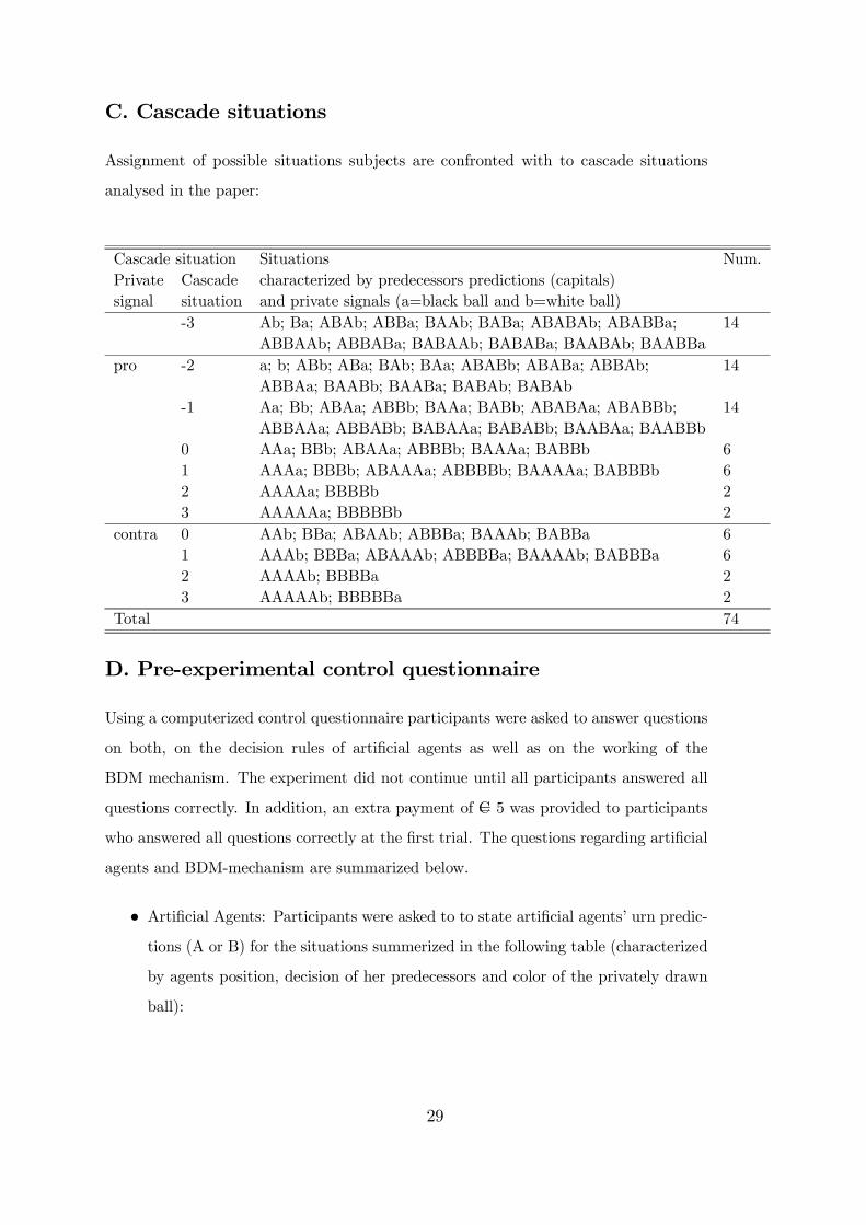
C. Cascade situations

Assignment of possible situations subjects are confronted with to cascade situations

analysed in the paper:

Cascade situation Situations Num.Private Cascade characterized by predecessors predictions (capitals)signal situation and private signals (a=black ball and b=white ball)

-3 Ab; Ba; ABAb; ABBa; BAAb; BABa; ABABAb; ABABBa; 14ABBAAb; ABBABa; BABAAb; BABABa; BAABAb; BAABBa

pro -2 a; b; ABb; ABa; BAb; BAa; ABABb; ABABa; ABBAb; 14ABBAa; BAABb; BAABa; BABAb; BABAb

-1 Aa; Bb; ABAa; ABBb; BAAa; BABb; ABABAa; ABABBb; 14ABBAAa; ABBABb; BABAAa; BABABb; BAABAa; BAABBb

0 AAa; BBb; ABAAa; ABBBb; BAAAa; BABBb 61 AAAa; BBBb; ABAAAa; ABBBBb; BAAAAa; BABBBb 62 AAAAa; BBBBb 23 AAAAAa; BBBBBb 2

contra 0 AAb; BBa; ABAAb; ABBBa; BAAAb; BABBa 61 AAAb; BBBa; ABAAAb; ABBBBa; BAAAAb; BABBBa 62 AAAAb; BBBBa 23 AAAAAb; BBBBBa 2

Total 74

D. Pre-experimental control questionnaire

Using a computerized control questionnaire participants were asked to answer questions

on both, on the decision rules of artificial agents as well as on the working of the

BDM mechanism. The experiment did not continue until all participants answered all

questions correctly. In addition, an extra payment of C= 5 was provided to participants

who answered all questions correctly at the first trial. The questions regarding artificial

agents and BDM-mechanism are summarized below.

• Artificial Agents: Participants were asked to to state artificial agents’ urn predic-tions (A or B) for the situations summerized in the following table (characterized

by agents position, decision of her predecessors and color of the privately drawn

ball):

29

No. Agents’ Predictions of Color of the Correctposition predecessors privately drawn ball answer

1 1 black A2 3 AB white B3 4 ABB black A4 4 AAA white A5 3 BA white B6 1 white B7 3 BB black B8 2 B black B

• Price Mechanism: Participants were asked to state whether they will participatein the urn prediction and the corresponding payment chances (Yes or No) and

to calculate the resulting income from the experiments in the situations sum-

merized the following table (characterized by maximum price, random price and

correctness of the urn prediction).

Max. price Random price Urn prediction Participation Resulting incomepmax pr (correct answer) (correct answer)60 71 correct No 050 35 wrong Yes - 3570 50 correct Yes 50

In addition, subjects were asked to state the optimal choice of the maximum price

assuming that they are willing to pay 50 ECU at maximum (correct answer: 50 ECU).

E. Further statistical analyses

E.1. Statistics on price setting behavior

In the following tables and describtives and test statistics are summerized for those 23

participants who

1. showed more than 95% of urn predictions in line with the BHW model and

2. answered all questions about artificial predecessors at the first time.

• Descriptive statistics of price setting behavior and subjective probability state-ments:

30

Individual average prices Ind. subj. probabilitiesPrivate Signal Cas. pos. Mean Median Std. dev. Mean Median Std.dev.

-3 30,36 28,57 19,11 42,27 46,79 12,14-2 38,06 24,28 17,20 49,13 51,21 10,67-1 54,00 54,29 18,12 60,43 61,64 9,600 60,34 61,00 22,09 66,34 66,67 12,19

Pro 1 69,42 77,50 21,37 76,67 76,67 10,992 70,76 75,00 20,52 62,98 77,50 31,743 72,78 80,00 21,66 64,43 82,50 31,990 39,92 40,83 15,82 47,61 50,00 12,07

Contra 1 50,25 50,00 19,47 58,65 60,00 12,452 55,00 52,50 23,31 52,08 62,50 26,313 63,98 70,00 25,40 57,55 69,00 29,46

• Friedman-test and Spearman rank correlations regarding price limits at differentcascade situations:

Friedman-test Spearman rank corr.Hypothesis (H0) χ2 (sign.) ρ (sign. 2-tailed)

a) p−3promax = p−2promax = p

−1promax = p

0promax 55.852 (.000) .509 (.000)

b) p0promax= p1promax= p

2promax= p

3promax 19.366 (.000) .208 (.046)

c) p0conmax= p1conmax= p

2conmax= p

3conmax 11.314 (.000) .367 (.000)

E.2. Statistics regarding subjective probabilities

• Friedman-test and Spearman rank correlations regarding subjective probabilitiesat different cascade situations:

Friedman-test Spearman rank corr.Hypothesis (H0) χ2 (sign.) ρ (sign. 2-tailed)

a) p−3promax = p−2promax = p

−1promax = p

0promax 92.937 (.000) .642 (.000)

b) p0promax= p1promax= p

2promax= p

3promax 68.809 (.000) .447 (.001)

c) p0conmax= p1conmax= p

2conmax= p

3conmax 69.033 (.000) .635 (.000)

31