DI

SC

US

SI

ON

P

AP

ER

S

ER

IE

S

Forschungsinstitut zur Zukunft der ArbeitInstitute for the Study of Labor

Do Female Executives Make a Difference?The Impact of Female Leadership on Gender Gaps and Firm Performance

IZA DP No. 8602

October 2014

Luca FlabbiMario MacisAndrea MoroFabiano Schivardi

Do Female Executives Make a Difference? The Impact of Female Leadership on Gender Gaps and Firm Performance

Luca Flabbi Inter-American Development Bank and IZA

Mario Macis

Johns Hopkins University and IZA

Andrea Moro Università Ca’ Foscari di Venezia and Vanderbilt University

Fabiano Schivardi

Bocconi University, IGIER, EIEF and CEPR

Discussion Paper No. 8602 October 2014

IZA

P.O. Box 7240 53072 Bonn

Germany

Phone: +49-228-3894-0 Fax: +49-228-3894-180

E-mail: iza@iza.org

Any opinions expressed here are those of the author(s) and not those of IZA. Research published in this series may include views on policy, but the institute itself takes no institutional policy positions. The IZA research network is committed to the IZA Guiding Principles of Research Integrity. The Institute for the Study of Labor (IZA) in Bonn is a local and virtual international research center and a place of communication between science, politics and business. IZA is an independent nonprofit organization supported by Deutsche Post Foundation. The center is associated with the University of Bonn and offers a stimulating research environment through its international network, workshops and conferences, data service, project support, research visits and doctoral program. IZA engages in (i) original and internationally competitive research in all fields of labor economics, (ii) development of policy concepts, and (iii) dissemination of research results and concepts to the interested public. IZA Discussion Papers often represent preliminary work and are circulated to encourage discussion. Citation of such a paper should account for its provisional character. A revised version may be available directly from the author.

IZA Discussion Paper No. 8602 October 2014

ABSTRACT

Do Female Executives Make a Difference? The Impact of Female Leadership on Gender Gaps and Firm Performance* We analyze a matched employer-employee panel data set and find that female leadership has a positive effect on female wages at the top of the distribution, and a negative one at the bottom. Moreover, performance in firms with female leadership increases with the share of female workers. This evidence is consistent with a model where female executives are better equipped at interpreting signals of productivity from female workers. This suggests substantial costs of under-representation of women at the top: for example, if women became CEOs of firms with at least 20% female employment, sales per worker would increase 6.7%. JEL Classification: M5, M12, J7, J16 Keywords: executives’ gender, gender gap, firm performance, glass ceiling,

statistical discrimination Corresponding author: Luca Flabbi Research Department Inter-American Development Bank 1300 New York Avenue NW Washington, DC 20005 USA E-mail: lucaf@iadb.org

* We thank Manuel Bagues, John Earle, Stephan Eblich, Nicola Lacetera, Giovanni Pica, Kathryn Shaw, and seminar participants at many conferences and institutions for very useful comments and suggestions. Partial funding from the Economic and Sector Work RG-K1321 at the IDB, the PRIN grant 2010XFJCLB_001 and the RAS L.7 project CUP: F71J11001260002 is gratefully acknowledged. The opinions expressed in this paper are those of the authors and do not necessarily reflect the views of the Inter-American Development Bank, its Board of Directors, or the countries they represent.

1 Introduction

This paper investigates how the gender of a firm’s CEO affects the workers’ gender-specific wage distributions and the firm’s performance using a unique matched em-ployer–employee panel dataset representative of the Italian manufacturing sector.

A growing literature shows that executives’ characteristics such as managementpractices, style, and attitudes towards risk can have an effect on firm outcomes.1 Ourfocus on gender follows from the abundant evidence of systematic gender differentialsin the labor market.2 Research has highlighted that women are almost ten times lessrepresented than men in top positions in firms.3 For example, recent U.S. data showthat even though women are a little more than 50% of white collar workers, theyrepresent only 4.6% of executives.4 Our own Italian data show that about 26% ofworkers in the manufacturing sector are women compared with only 3% of executivesand 2% of CEOs. Together, these facts suggest that gender is a potentially relevantcharacteristic and that women’s under-representation among executives may haveimportant productivity and welfare implications.

This paper provides four contributions to the existing literature. First, we de-velop a theoretical model highlighting a potential channel of interaction betweenfemale executives, female workers, wage policies, job assignment, and overall firmperformance. The model implies efficiency costs of women’s under-representationin leadership positions, and generates empirical predictions that can be tested andcompared with implications from possible alternative mechanisms. Second, we in-vestigate the empirical predictions of the model for the relationship between femaleleadership and the gender-specific wage distributions at the firm level. Different

1Bloom and Van Reenen (2007) is one of the first contributions emphasizing differences inmanagement practices. See also a recent survey in Bloom and Van Reenen (2010). A growingliterature showing the effects of CEO characteristics follows the influential paper of Bertrand andSchoar (2003). Among recent contributions, see Bennedsen et al. (2012), Kaplan et al. (2012), orLazear et al. (2012). For research on executives’ overconfidence, see Malmendier and Tate (2005).For theoretical contributions, see for example Gabaix and Landier (2008) and Tervio (2008). Forcontributions focusing on both executive and firm characteristics, see Bandiera et al. (2011) andLippi and Schivardi (2014).

2For an overview of the gender gap in the U.S. labor market in the last twenty years, see Blauand Kahn (2004), Eckstein and Nagypal (2004) and Flabbi (2010).

3Evidence from U.S. firms is based on the Standard and Poor’s ExecuComp dataset, whichcontains information on top executives in the S&P 500, S&P MidCap 400, and S&P SmallCap 600.See for example, Bertrand and Hallock (2001), Wolfers (2006), Gayle et al. (2012), Dezsö and Ross(2012). The literature on other countries is extremely thin: see Cardoso and Winter-Ebmer (2010)(Portugal), Ahern and Dittmar (2012) and Matsa and Miller (2013) (Norway), Smith et al. (2006)(Denmark). A related literature is concerned with under-representation of women at the top of thewage distribution, see for example Albrecht et al. (2003). Both phenomena are often referred to asa glass-ceiling preventing women from reaching top positions in the labor market.

4Our elaboration on 2012 Current Population Survey and ExecuComp data.

1

from previous literature, and consistent with our model, the main focus is not onthe effects on average wages, but on differential impacts over the wage distribution.This is important because different theoretical mechanisms have different predic-tions for what the effects of female leadership should be at different parts of thewage distribution. Third, we investigate the empirical predictions of the model onthe relationship between female leadership and firm performance. Unlike previousliterature, which focused generally on measures of financial performance, we focuson indicators that are less volatile and less likely to be affected by gender discrimina-tion: sales per worker, value added per worker and Total Factor Productivity (TFP)(Wolfers, 2006). Finally, we perform a series of partial equilibrium counterfactualexercises to compute the cost of women’s under-representation in top positions inorganizations.

In Section 2 we present our theoretical model and derive its empirical implica-tions. Our model extends the seminal statistical discrimination model of Phelps(1972) to include two types of jobs, one requiring complex tasks and the other sim-ple tasks, and two types of CEOs, male and female. Based on a noisy productivitysignal and the worker’s gender, CEOs assign workers to jobs and wages. We assumethat CEOs are better (more accurate) at reading signals from workers of their owngender.5 We also assume that complex tasks require more skills to be completedsuccessfully, and that there is a comparative advantage to employ higher humancapital workers in complex tasks. After defining the equilibrium generated by thisenvironment, we focus on the empirical implications of a female CEO taking chargeof a male CEO-run firm. Thanks to the more precise signal they receive from femaleworkers, female CEOs reverse statistical discrimination against women, adjustingtheir wages and reducing the mismatch between female workers’ productivity andjob requirements. The model delivers two sharp, testable empirical implications:

1. Females at the top of the wage distribution receive higher wages when employedby a female CEO than when employed by a male CEO. Females at the bottomof the wage distribution receive lower wages when employed by a female CEO.The impact of female CEOs on the male distribution has the opposite signs:negative at the top and positive at the bottom of the distribution.

2. The performance of a firm led by a female CEO increases with the share offemale workers.

These results follow from the assumption that female CEOs are better at processinginformation about female workers’ productivity. Therefore, wages of females em-

5We discuss this assumption in Subsection 2.3.

2

ployed by female CEOs are more sensitive to individual productivity, delivering thefirst implication. Moreover, female CEOs improve the allocation of female workersacross tasks, delivering the second implication.

Our data, described in detail in Section 3, includes all workers employed by firmswith at least 50 employees in a representative longitudinal sample of Italian manu-facturing firms between 1982 and 1997.6 Because we observe all workers and theircompensation, we can evaluate the impact of female leadership on the wage distri-bution at the firm level. The data set is rich in firm-level characteristics, includingseveral measures of firm performance. We merge this sample with social securityadministration data containing the complete labor market trajectories of all workerswho ever transited through any of the sampled firms. This allows us to identifyfirm, worker and executive fixed effects in a joint two-way fixed effects regressionsà la Abowd et al. (1999) and Abowd et al. (2002). These fixed effects and controlshelp address the scarcity of worker-level characteristics in our data set, and allow usto control for unobservable heterogeneity at the workforce, firm and executive levelwhich would otherwise bias the estimates.

We describe our empirical strategy and present the estimation results in Section4. Thanks to the richness of our data, we can analyze the impact on the entire wagedistribution within the firm allowing for heterogenous effects across workers. Ourregressions by wage quantiles show that this heterogeneity is relevant: the impactof having a female CEO is positive on women at the top of the wage distributionbut negative on women at the bottom of the wage distribution. These effects areconsistent with our model, and not consistent with alternative mechanisms throughwhich female CEOs could affect women’s wages, as we discuss in detail in Section5. Also, consistent with our model’s predictions, female CEOs are associated withlower wages for men at the top, and higher wages for men at the bottom of thewage distribution. As a result, we find that, as implied by our model, female CEOsreduce the gender wage gap at the top and widen it at the bottom of the wagedistribution, with essentially no effects at the mean. Our results are robust toalternative specifications, such as an alternative measure of female leadership (theproportion of the firm’s executives who are female) and to the selection induced byentry and exit of firms and workers.

We also analyze the impact of female leadership on firm performance, measuredby sales per worker, value added per worker, and total factor productivity (TFP).Results confirm the our model’s prediction: the impact of female CEOs on firm

6This is the only period over which our data are available and this is the reason why we cannotprovide an analysis using more recent data.

3

performance is a positive function of the proportion of female workers employed bythe firm. The magnitude of the impact is substantial: a female CEO would increaseoverall sales per employee by about 3.7% if leading a firm employing the averageproportion of women.

Using our estimates, we perform a partial equilibrium counterfactual exerciseto compute the cost of women’s under-representation in leadership positions. Ourresults indicate that if female CEOs were in charge of all firms with at least a 20%proportion of female workers (about 50 percent of the sample), sales per workerwould increase by 14% in the “treated” firms, and by 6.7% in the overall sample offirms.

There is a large literature studying gender differentials in the labor market, anda fairly developed literature studying gender differentials using matched employer-employee data. However, the literature on the relationship between the gender ofthe firm’s executives and gender-specific wages is scant and has focused on the effecton average wages, not on the effect over the entire wage distribution. Bell (2005)studies the impact of female leadership in US firms but only on executives’ wages.Cardoso and Winter-Ebmer (2010) consider the effect on all workers in a sample ofPortuguese firms but without allowing for heterogeneous effects over the distribution.Fadlon (2010) tests a model of statistical discrimination similar to ours and assessesthe impact of supervisors’ gender on workers’ wages using U.S. data but does notfocus on the wage distribution and does not look at wages at the firm level. Gagliar-ducci and Paserman (2014) use German linked employer-employee data to study theeffect of the gender composition of the first two layers of management on firm andworker outcomes. They find that the effect of female leadership is heterogeneousand depends on the share of women in the second layer of the organization: Womenin the top layer who are surrounded by men reduce wages of both men and women,while the effect is reversed as the share of women in the second layer increases. Arelated literature, sparked by recent reforms in European countries, looks at theimpact of the gender of a firm’s board members instead of its executives. Bertrandet al. (2014) documents that a reform mandating gender quotas for the boards ofNorwegian companies reduced the gender gap in earnings within board members butdid not have a significant impact on overall gender wage gaps.

Existing literature on the effect of female leadership on firm performance is alsolimited. Many contributions focus on financial performance looking at the impacton stock prices, stock returns and market values.7 By conditioning on a wide range

7See for example, Wolfers (2006), Albanesi and Olivetti (2009), Ahern and Dittmar (2012); inthe strategy literature, Dezsö and Ross (2012), Adams and Ferreira (2009), Farrell and Hersch(2005). Rare exceptions are Matsa and Miller (2013), which looks at operating profits, Smith et al.

4

of firm-level controls and using less volatile measures of firm performance, we canrun firm-level regressions closer to our model’s implications.

2 Theoretical Framework

We present a simple signal extraction model where inequalities are generated by em-ployers’ incomplete information about workers’ productivity and where employers’gender matters. The main assumption of our model is that female and male execu-tives are better equipped at assessing the skills of employees of their same gender. Asdiscussed in greater detail below, this may be the result of better communication andbetter aptitude at interpersonal relationships among individuals of the same gender,of more similar cultural background shared by individuals of the same gender, orother factors. From the model we derive a set of implications that we test in ourempirical analysis.

2.1 Environment

We extend the standard statistical discrimination model in Phelps (1972) to in-clude two types of employers (female and male), and two types of jobs (simple andcomplex). The two-jobs extension allows us to obtain implications for efficiency(productivity), which is one focus of our empirical analysis.8 Female (f) and male(m) workers have ability q which is distributed normally with mean µ and variance�2. Ability, productivity and wages are expressed in logarithms. CEOs observe asignal of ability s = q+ ✏, where ✏ is distributed normally with mean 0 and variance�2✏g where g is workers’ gender m or f . The signal’s variance can be interpreted as a

measure of the signal’s information quality. Employers assign workers to one of twojobs: one requiring complex (c) tasks to be performed and the other requiring simpletasks (e) to be performed. To capture the importance of correctly assigning workersto tasks, we assume that mismatches are costlier in the complex job, where workerswith higher ability are more productive. One way to model this requirement is byassuming that the dollar value of productivity of workers in the complex (simple)job is h (l) if workers have ability q > q, and �h (�l) otherwise, with h > l � 0.9

(2006), with information on value added and profits on a panel of Danish firms, and Rose (2007),which looks at Tobin’s Q.

8In the standard model of Phelps (1972) discrimination has a purely redistributive nature. Ifemployers were not allowed to use race as a source of information, production would not increase,but this is due to the extreme simplicity of the model. See Fang and Moro (2011) for details.

9The threshold rule for productivity is a strong assumption, which we adopted to simplify thederivation of the model’s outcome, but it is not crucial. What is crucial is that productivity increaseswith ability, and that lower ability workers are more costly mismatched in the complex job.

5

Firms compete for workers and maximize output given wages. Workers care onlyabout wages and not about job assignment per se.

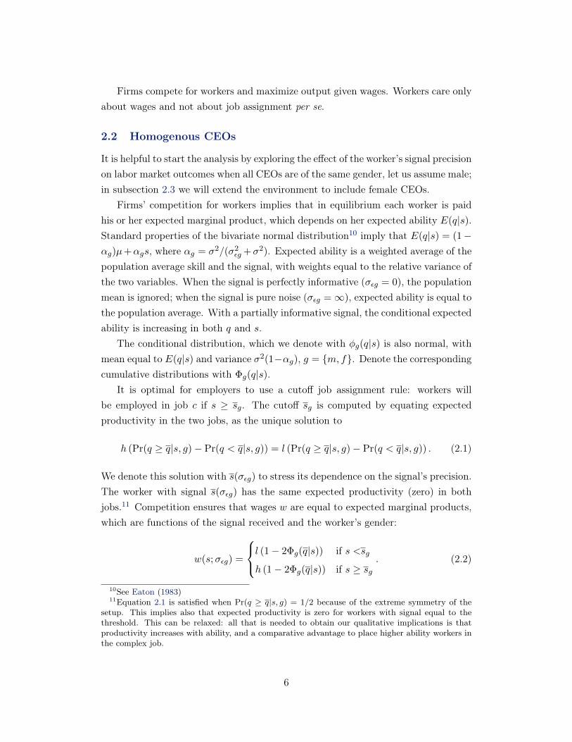
2.2 Homogenous CEOs

It is helpful to start the analysis by exploring the effect of the worker’s signal precisionon labor market outcomes when all CEOs are of the same gender, let us assume male;in subsection 2.3 we will extend the environment to include female CEOs.

Firms’ competition for workers implies that in equilibrium each worker is paidhis or her expected marginal product, which depends on her expected ability E(q|s).Standard properties of the bivariate normal distribution10 imply that E(q|s) = (1�↵g)µ+↵gs, where ↵g = �2/(�2

✏g +�2). Expected ability is a weighted average of the

population average skill and the signal, with weights equal to the relative variance ofthe two variables. When the signal is perfectly informative (�✏g = 0), the populationmean is ignored; when the signal is pure noise (�✏g = 1), expected ability is equal tothe population average. With a partially informative signal, the conditional expectedability is increasing in both q and s.

The conditional distribution, which we denote with �g(q|s) is also normal, withmean equal to E(q|s) and variance �2

(1�↵g), g = {m, f}. Denote the correspondingcumulative distributions with �g(q|s).

It is optimal for employers to use a cutoff job assignment rule: workers willbe employed in job c if s � sg. The cutoff sg is computed by equating expectedproductivity in the two jobs, as the unique solution to

h (Pr(q � q|s, g)� Pr(q < q|s, g)) = l (Pr(q � q|s, g)� Pr(q < q|s, g)) . (2.1)

We denote this solution with s(�✏g) to stress its dependence on the signal’s precision.The worker with signal s(�✏g) has the same expected productivity (zero) in bothjobs.11 Competition ensures that wages w are equal to expected marginal products,which are functions of the signal received and the worker’s gender:

w(s;�✏g) =

8<

:l (1� 2�g(q|s)) if s <sg

h (1� 2�g(q|s)) if s � sg. (2.2)

10See Eaton (1983)11Equation 2.1 is satisfied when Pr(q � q|s, g) = 1/2 because of the extreme symmetry of the

setup. This implies also that expected productivity is zero for workers with signal equal to thethreshold. This can be relaxed: all that is needed to obtain our qualitative implications is thatproductivity increases with ability, and a comparative advantage to place higher ability workers inthe complex job.

6

Signal

Wag

es

⌧4.0 2.0 3.5 10.0

⌧1.

0⌧

0.5

0.0

0.5

1.0

1.5

2.0

σε = 1(more precise signal)

σε = 2(less precise signal)

Figure 1: Simulation of the solution to the problem with parameters �=1,q = 1.5, µ = 1, h = 2, l = 1.

We now explore the properties of the wage schedule as a function of the signal’snoise variance �2

✏g. Figure 1 displays the outcome for workers with two differentvalues of �2

✏g. The red continuous line displays the equilibrium wages resulting froma more precise signal than the blue dashed line. As standard in statistical discrim-ination models, the line corresponding to the more precise signal is steeper thanthe line corresponding to the less precise signal. This is the direct implication ofputting more weight on the signal in the first case than in the second. As a result ofone of our extensions - the presence of job assignment between simple and complexjobs - the two lines also display a non-standard feature: a kink in correspondence tothe threshold signal. The kink is a result of the optimal assignment rule: workerswith signals below the threshold are assigned to the simple job, where ability affectsproductivity less than in the complex job, therefore both wage curves are flatter tothe left of the thresholds than to the right of the thresholds.

The following proposition states that the expected marginal product of a workeris higher when the signal is noisier if the signal is small enough. Conversely, fora high enough signal, the expected marginal product will be lower the noisier thesignal. Formally,

Proposition 1. Let w(s;�✏g) be the equilibrium wage as a function of the workers’

7

signal for group g, extracting a signal with noise standard deviation equal to �✏g.If �✏f > �✏m then there exists bs such that w(s;�✏f ) > w(s;�✏m) for all s < bs andw(s;�✏f ) < w(s;�✏m) for all s > bs.

The proof is in Appendix A.12 The next proposition states that productivity ishigher when the signal is more precise. This follows observing that expected abilityis closer to the workers’ signal when �2

✏g is smaller.

Proposition 2. Let yg(�✏g) be the total production of workers from group g whentheir signal’s noise has standard deviation �✏g. Production yg is decreasing in �✏g.

For example, with the parameters used in Figure 1, and assuming that femaleworkers are those with the larger signal noise variance (�✏m= 1 and �✏f = 2), 24percent of males and 13.2 percent of females are employed in the complex job. Be-cause there are fewer females than males in the right tail of the quality distributionconditional on any given signal, more females are mismatched, therefore males’ totalvalue of (log) production is equal to -0.29, whereas females’ is -0.35. To assess theinefficiency cost arising from incomplete information, consider that if workers wereefficiently assigned, the value of production would be 1.31 for each group.

2.3 Heterogenous CEOs: Female and Male

Consider now an environment in which some firms are managed by female CEOsand some by male CEOs.13 We assume that female CEOs are characterized by abetter ability to assess the productivity of female workers, that is, female workers’signal is extracted from a more precise distribution, with noise variance �2

✏F < �2✏f

(where the capital F denotes female workers when assessed by a female CEO, andlowercase f when assessed by a male CEO). Symmetrically, female CEOs evaluatemale workers’ with lower precision than male CEOs: �2

✏M > �2✏m.

This assumption may be motivated by any difference in language, verbal andnon-verbal communication styles and perceptions that may make it easier betweenpeople of the same gender to provide a better understanding of personal skills andattitudes, improve conflict resolutions, assignment to job-tasks, etc. A large socio-linguistic literature has found differences in verbal and non-verbal communication

12This “single-crossing” property of the wage functions of signals of different precision relies onassuming symmetry of the production function and of the signaling technology. However the resultthat a more precise signal implies higher wages at the top of the distribution, and lower wages atthe bottom, is more general, and holds even if the wage functions cross more than once.

13We do not model the change in CEO gender or how the CEO is selected as we are inter-ested in comparing differences in gender-specific wage distributions between firms where the topmanagement has different gender.

8

styles between groups defined by race or gender that may affect economic and socialoutcomes (see e.g. Dindia and Canary (2006) and Scollon et al. (2011)).14 Recentemployee surveys also indicate that significant communication barriers between menand women exist in the workplace (Angier and Axelrod (2014), Ellison and Mullin(2014)). In the economics literature, several theoretical papers have adopted an as-sumption similar to ours. Lang (1986) develops a theory of discrimination based onlanguage barriers between “speech communities” defined by race or gender. To moti-vate this assumption, Lang surveys the socio-linguistic literature demonstrating theexistence of such communication barriers. Cornell and Welch (1996) adopt the sameassumption in a model of screening discrimination. Morgan and Várdy (2009) dis-cuss a model where hiring policies are affected by noisy signals of productivity, whoseinformativeness depends (as in our assumption) on group identity because of differ-ences in “discourse systems”. More recently, Bagues and Perez-Villadoniga (2013)’smodel generates a similar-to-me-in-skills result where employers endogenously givehigher valuations to candidates who excel in the same dimensions as them. Thisresult can also provide a foundation to our assumption if female workers are morelikely to excel on the same dimensions as female executives.

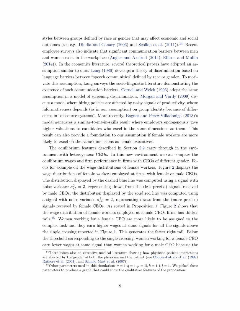
The equilibrium features described in Section 2.2 carry through in the envi-ronment with heterogenous CEOs. In this new environment we can compare theequilibrium wages and firm performance in firms with CEOs of different gender. Fo-cus for example on the wage distributions of female workers. Figure 2 displays thewage distributions of female workers employed at firms with female or male CEOs.The distribution displayed by the dashed blue line was computed using a signal withnoise variance �2

✏f = 3, representing draws from the (less precise) signals receivedby male CEOs; the distribution displayed by the solid red line was computed usinga signal with noise variance �2

✏F = 2, representing draws from the (more precise)signals received by female CEOs. As stated in Proposition 1, Figure 2 shows thatthe wage distribution of female workers employed at female CEOs firms has thickertails.15 Women working for a female CEO are more likely to be assigned to thecomplex task and they earn higher wages at same signals for all the signals abovethe single crossing reported in Figure 1. This generates the fatter right tail. Belowthe threshold corresponding to the single crossing, women working for a female CEOearn lower wages at same signal than women working for a male CEO because the

14There exists also an extensive medical literature showing how physician-patient interactionsare affected by the gender of both the physician and the patient (see Cooper-Patrick et al. (1999)Rathore et al. (2001), and Schmid Mast et al. (2007)).

15Other parameters used in this simulation: � = 1, q = 1, µ = .5, h = 1.1, l = 1. We picked theseparameters to produce a graph that could show the qualitative features of the proposition.

9

Female wages

Den

sity

Female CEOs (more precise signal)

Male CEOs (less precise signal)

⌧1 0 1 2

0.0

0.5

1.0

1.5

Figure 2: Simulation of the wage distributions of female workers

female CEO has a better assessment of how low productivity really is in those cases.This generates the fatter left tail. The following prediction follows directly fromProposition 1:

Empirical implication 1. Wages of female workers in firms with female CEOs arehigher at the top of the wage distribution, and lower at the bottom of the wage distri-bution relative to wages of female workers employed by male CEOs. Symmetrically,wages of male workers in firms with female CEOs are higher at the bottom and lowerat the top of the wage distribution relative to wages of male workers employed bymale CEOs.

As a result, and as Figure 2 makes clear, we should also expect the variance ofthe wage distribution of female workers employed by female CEOs to be higher thanthe variance of the wage distribution of female workers employed by male CEOs.The opposite should be true on the variance of male wages.

The model has implications for firm performance as well. Proposition 2 statesthat total production is higher the lower the signal noise since CEOs can better matchworkers to jobs. As a result, we should observe that female CEOs can improve firmperformance by implementing a better assignment of female workers.16 Therefore,

16Symmetrically, female CEO’s assignment of male workers has the opposite effect. However,

10

we will test the following empirical prediction:

Empirical implication 2. The productivity of firms with female CEOs increaseswith the share of female workers.

We derived Propositions 1 and 2 using specific distributional assumptions, butthe empirical implications are robust to alternative distributions of the signal’s noiseand of the underlying productivity. A higher signal precision always implies less mis-matching of workers to jobs, and a higher correlation of signals with productivityalways implies lower wages when the signal is small and higher wages when the signalis high. These implications are also robust to alternative specifications of the signalextraction technology. In the online appendix (Flabbi et al. (2014)), we derive thesame empirical implications assuming a dynamic model where signals are extractedevery period. Assuming all firms initially have male CEOs, firms acquiring femaleCEOs update the expected productivity of female workers with higher precision.The implications follow because female CEOs will rely on a larger number of moreprecise signals from female workers than male CEOs.

We do not model explicitly the selection process into executive positions (al-though in the empirical part we will take into account that such process might differby gender) or how labor force dynamics are affected by CEO gender in a “generalequilibrium”. The change of a CEO’s gender in our model will affect incentives forworkers to leave the firm hoping to extract a more advantageous signal. Our resultstherefore assume rigidities in workforce mobility, which can be motivated by costs ofhiring and firing. However, the equilibrium wages by CEO and worker’s gender de-rived in our propositions are nevertheless optimal and are indicative of the directionsof wage changes we should expect when a CEO of different gender is appointed.17

3 Data and Descriptive Statistics

3.1 Data Sources and Estimation Samples

We use data from three sources that we label INVIND, INPS and CADS. Fromthese three sources of data, we build a matched employer-employee panel data setand from this matched data set we extract our final estimation samples.

this effect might be weakened if female CEOs, upon assuming leadership, could “trust” the previousassignment of male workers made by a male CEO. We are agnostic about the details of job reas-signment of workers of a different gender, which we do not model, and we focus on an implicationthat is robust to such details.

17This motivates in the empirical analysis the inclusion, in our benchmark specification, only ofdata from workers that were not hired after the new CEO was appointed. We check the robustnessof our results to the inclusion of all workers.

11

INVIND stands for the Bank of Italy’s annual survey of manufacturing firms,an open panel of about 1,000 firms per year, representative of Italian manufactur-ing firms with at least 50 employees. INPS stands for the National Social Secu-rity Institute which provided the work histories of all workers ever employed at anINVIND firm in the period 1980-1997,18 including spells of employment in firmsnot included in the INVIND survey. We match the INVIND firms with the INPSwork histories thanks to unique worker and firms identifiers to create what we callthe INVIND-INPS data set. This data set includes for each worker: gender, age,tenure19, occupational status (production workers, non-production workers, execu-tives), annual gross earnings (including overtime pay, shift work pay and bonuses),number of weeks worked, and a firm identifier. We exclude all records with missingentries on either the firm or the worker identifier, those for workers younger than15, and those corresponding to workers with less than four weeks worked in a givenyear. For each worker-year, we kept only the observation corresponding to the mainjob (the job with the highest number of weeks worked). Overall, the INVIND-INPSdata set includes information on about a million workers per year, more than halfof whom are employed in INVIND firms in any given year. The remaining workersare employed in about 450,000 other companies of which we only know the firmidentifier.

In Table 1 we report summary statistics on workers’ characteristics for theINVIND-INPS data set. About 67% of observations pertain to production work-ers, 31% to non-production employees, and 2.2% to executives. Even though theyrepresent about 21% of the workforce, women are only 2.5% of executives. On av-erage, workers are 37 years old and have 5 years of tenure. Average gross weeklyearnings at 1995 constant prices are around 388 euros, with women earning about24% less than men (309 euros vs. 408 euros).

CADS, the third data source we use, stands for Company Accounts Data Serviceand includes balance-sheet information for a sample of about 40,000 firms between1982 and 1997, including almost all INVIND firms. The data include informationon industry, location, sales, revenues, value added at the firm-year level, and a firmidentifier. Again thanks to a unique and common firm identifier, we can matchCADS with INVIND-INPS.

We will focus most of our empirical analysis on the balanced panel sample con-18The provision of these work histories data for the employees of the INVIND firms was done

only once in the history of the data set and therefore can only cover firms and workers up to 1997.This is the reason why we cannot work on more recent data.

19Tenure information is left-censored because we do not have information on workers prior to1981.

12

sisting of firms continuously observed in the period 1988-1997. In Table 1 we reportsummary statistics both on this sample and on the entire, unbalanced INVIND-INPS-CADS sample for the same period. Notice that the unit of observation on thesample is a firm in a given year while in the INVIND-INPS was a worker in a givenfirm in a given year. The unbalanced INPS-INVIND-CADS panel includes 5,029firm-year observations from a total of 795 unique firms. Of these, 234 compose thebalanced panel. In the unbalanced sample, average gross weekly earnings at 1995constant prices are equal to about 405 euros. On average, workers are 37.2 years oldand have 8 years of tenure in the firm. About 68% of the workers are blue collar, 30%white collar, and 2.5% are executives. The corresponding statistics in the balancedsample are very similar.

3.2 Female Leadership

We identify female leadership from the job classification executive20 in the data. Asalready observed by Bandiera et al. (2011), one advantage of using data from Italyis that this indicator is very reliable because the job title of executive is subject toa different type of labor contract and executives are registered in a separate accountwith the social security administration agency (INPS). We identify the CEO as theexecutive with the highest compensation in a firm-year. This procedure is supportedby the following: i) Salary determination in the Italian manufacturing sector is suchthat the compensation ordering follows very closely the hierarchical ranking withineach of the three broad categories we observe (executives, non-production workers,production workers); ii) The firm’s CEO is classified within the executive category;iii) We have a very detailed and precise measure of compensation because we havedirect access to the administrative data that each firm is required by law to report(and that each worker has the incentive to verify is correctly reported); iv) We haveaccess to all the workers employed by a given firm in a given year.21

Using these definitions, we find that although females are 26.2% of the workforcein INVIND firms, they are only 3.3% of the executives, and only 2.1% of CEOs. Thedescriptive statistics for the balanced panel are quite similar to those referring to theunbalanced sample and confirm the under-representation of women in top positionsin firms found for other countries. In particular, the ratio between women in the

20The original job description in Italian is dirigente, which corresponds to an executive in a USfirm.

21We have the complete set of workers only for the INVIND firms and as a result we can onlyassign CEO’s gender to INVIND firms. However, this is irrelevant for our final estimation sampleat the firm level since for other reasons explained below we limit our main empirical analysis to asubset of INVIND firms.

13

Table 1: Descriptive statistics: INVIND-INPS sample and INVIND-INPS-CADS sample

INVIND-INPS INVIND-INPS-CADSUnbalanced Balanced

panel panelMean Std.Dev. Mean Std.Dev. Mean Std.Dev.

% Prod. workers 66.5 67.6 (18.7 ) 67.4 (18.3)% Non-prod. wrk 31.3 29.8 (17.7) 30.0 (17.3)

% Executives 2.2 2.5 (1.7) 2.6 (1.8)% Females 21.1 26.2 (20.9) 25.8 (20.1)

% Fem. execs. 2.5 3.3 (10.3) 3.4 (10.1)% Female CEO 2.1 1.8

Age 37.0 (10.1) 37.2 (3.6) 37.4 (3.4)Tenure 5.1 (4.1) 8.1 (2.6) 8.7 (2.3)

Wage (weekly) 387.2 (253.8) 400.3 (86.0) 404.5 (88.7)Wage (males) 408.1 (271.8) 429.3 (92.7) 433.9 (97.5)

Wage (females) 309.5 (146.6) 343.3 (67.0) 346.4 (68.5)

Firm size (empl.) 675.0 (2,628.6) 704.2 (1,306.9)Sales (’000 euros) 110,880 (397,461) 118,475 (231,208)Sales/worker (ln) 4.93 (0.62) 4.95 (0.57)

Val. add./wkr (ln) 3.77 (0.43) 3.79 (0.41)TFP 2.49 (0.50) 2.49 (0.49)

N. Observations 18,664,304 5,029 2,340N. Firms 448,284 795 234

N. Workers 1,724,609N. Years 17 15 10

labor force and women classified as executives is very similar to the ratio obtainedfrom the ExecuComp22 data for the U.S.

Women’s representation in executive positions in Italy has increased over timebut remains small: In 1980, slightly above 10 percent of firms had at least one femaleexecutive, and females represented 2% of all executives and 1% of CEOs; In 1997,these figures were 20%, 4% and 2%, respectively. There is substantial variationacross industries in the presence of females in the executive ranks, but no obviouspattern emerges about the relationship between female leadership and the presence

22Execucomp is compiled by Standard and Poor and contains information on executives in theS&P 500, S&P MidCap 400, S&P SmallCap 600. See for example, Bertrand and Hallock (2001),Wolfers (2006), Gayle et al. (2012), Dezsö and Ross (2012).

14

Table 2: Descriptive statistics: Firms with Male and Female CEO inINVIND-INPS-CADS sample

Male CEO Female CEOMean St.Dev. Mean St.Dev.

CEO’s age 49.5 (7.1) 46.6 (7.1)CEO’s tenure 4.4 (3.7) 4.0 (2.8)

CEO’s annual earnings 199,385 (144,508) 128,157 (54,643)

% Production workers 67.5 (18.7) 75.4 (13.5)% Non-prod. workers 30.0 (17.8) 22.2 (13.1)

% Executives 2.5 (1.7) 2.4 (1.4)% Females 25.9 (20.7) 37.2 (27.0)

% Female executives 2.4 (6.9) 46.8 (29.5)% Female executives (excl. CEO) 3.3 (10.3) 15.9 (28.6)

Firm size (employment) 683.7 (2,655.4) 270.3 (409.9)Age 37.2 (3.6) 35.9 (3.5)

Tenure 8.1 (2.6) 8.6 (2.2)Wage (earnings/week) 401.6 (86.0) 341.3 (61.7)

Wage (males) 430.6 (92.8) 369.4 (64.2)Wage (females) 343.3 (66.2) 345.4 (97.1)

Sales (thousand euros) 112,467 (401,486) 37,185 (55,982)Sales per worker (ln) 4.9 (0.6) 4.7 (0.6)

Value added per worker (ln) 3.8 (0.4) 3.6 (0.4)TFP 2.5 (0.5 ) 2.4 (0.5)

N. Observations 4,923 106N. Firms 788 60 33N. Years 15 10

of females in the non-executive workforce in the various industries.23

In Table 2 we compare firms with a male CEO with those with a female CEO.Firms with a female CEO are smaller, both in terms of employment and in terms ofrevenues, pay lower wages, and employ a larger share of blue collar workers. Firmswith a female CEO also employ a larger share of female workers (37 vs. 26 percent).However, when one looks at measures of productivity (sales per employee, valueadded per employee, and TFP), the differences shrink considerably. For instance,total revenue is on average about 3 times higher in firms with a male CEO than infirms with a female CEO, but revenue per employee, value added per employee and

23See Table B1 in Flabbi et al. (2014) for details.

15

TFP are only about 21 percent, 19 percent and 4 percent higher, respectively.

4 Empirical Analysis

4.1 Specification and Identification

The unit of observation of our analysis is a given firm j observed in a given year t.We are interested in the impact of female leadership on workers’ wage distributionsand firms’ performance.

We will estimate regressions of the following form:

yjt = �FLEADjt+FIRM 0jt�+WORK 0

jt�+EXEC 0jt�+�j+⌘t+⌧t(j)t+"jt (4.1)

where: yjt is the dependent variable of interest (either moments of the workers’ wagedistribution or measures of firm performance) and � is the coefficient of interest. Theregressors and controls are defined as follows: FLEADjt is the measure of femaleleadership used in the regression: either a female CEO dummy or the fraction offemale executives; FIRMjt is a vector of observable time-varying firm character-istics (dummies for size, industry, and region); WORKjt is a vector of observableworkforce characteristics aggregated at the firm-year level (age, tenure, occupationdistribution, fraction female) plus worker fixed effects aggregated at the firm-yearlevel and estimated in a “first stage” regression described in detail below; EXECjt

is a vector of observable characteristics of the firm leadership used in the regres-sion (age and tenure as CEO or executive) plus CEO’s or executives’ fixed effectsestimated in the first stage regression described in detail below;24 �j are firm fixedeffects; ⌘t are year dummies and ⌧t(j) are industry-specific time trends.

The main challenge in estimating the impact of female CEOs (or female leader-ship in general)25 on workers’ wages and firms’ performance is the sample selectionbias induced by the non-random assignment of CEOs to firms. In particular, it ispossible that (a) unobservable firm characteristics may make some firms more pro-ductive than others, and this unobserved firm-level component may not be randomlyassigned between male- and female-led firms, (b) the workforce composition of firmsled by women might systematically differ from that of firms led by men, and (c)the selection on unobserved individual ability in the position of CEO may not be

24When the female leadership measures is the female CEO dummy we simply use the CEO’svalue of the listed regressors; when the leadership measure is the proportion of female executivesat the firms, we use the average of the listed regressors over the firm’s executives.

25To simplify the discussion, we present the identification for the case in which female leadershipis represented by the dummy female CEO. The same discussion carries through when we use thefraction of female executives as a measure of female leadership.

16

the same by gender so that women CEOs may be of systematically higher or lowerability than men CEOs, and female leadership indicators might be capturing suchdifferences rather than gender effects.

Our strategy to address these issues is to control for firm fixed effects, workforcecomposition effects, and CEO effects. Thanks to the panel structure of the data, wecan control for time-invariant firm-level heterogeneity by estimating equations (4.1)as firm fixed effects regressions; we can also include controls for a set of time-varying,observable firm characteristics, workforce characteristics, and CEO characteristics.Moreover, as we describe in the next paragraph, we exploit the employer-employeenature of our data to construct controls for unobservable workforce and CEO ability.

Our matched employer-employee data includes the entire work history of all theworkers who ever transited through one of our J INVIND firms. This large matchedemployer-employee data set (almost 19 million worker-year observations) containsa large number of transitions of individuals across (INVIND and non-INVIND)firms and is thus well suited to estimate two-way fixed effects as in Abowd et al.(1999)(henceforth, AKM). An individual fixed effect estimated from such a regres-sion has the advantage of controlling for the firms the worker or executive has everworked for. As a result, it can capture those scale effects in individual productiv-ity which are usually captured by education, other time-invariant human capital orother proxies for “ability” and skills.26

Our strategy is to use the individual fixed effects from an AKM regression to con-struct proxies for CEO/executive and average worker heterogeneity at the firm-yearlevel to include as controls in regression 4.1. Specifically, we perform the two-wayfixed effect procedure proposed by Abowd et al. (2002) by estimating the followingequation:

wit = s0it� + ⌘t + ↵i +

JX

j=1

djit j + ⇣it. (4.2)

The dependent variable is the natural logarithm of weekly wages. The vector ofobservable individual characteristics, s0, includes age, age squared, tenure, tenuresquared, a dummy variable for non-production workers, a dummy for executives(occupational status changes over time for a considerable number of workers), aswell as a full set of interactions of these variables with a female dummy (to allow thereturns to age, tenure and occupation to vary by gender), and a set of year dummies.Our original sample consists of essentially one large connected group (comprising 99%

26Including these controls as described in detail below also helps alleviate the fact that our dataset, as is frequently the case with administrative data, does not include a particularly rich set ofcontrols at the individual worker level. For example, we have no measure of education or otherformal training in the data which are usually included as controls in wage regressions.

17

of the sample). Thus, in our estimation we focus only on this connected group anddisregard the remaining observations. The identification of firm effects and workereffects is delivered by the relatively high mobility of workers in the sample over therelatively long period under consideration: about 70 percent of workers have morethan one employer during the 1980-1997 period, and between 8 and 15 percent ofworkers change employer in a given year. The ↵̂i obtained by this procedure for thefirms’ CEOs and executives are included in the vector EXECjt to control for CEO’sindividual heterogeneity. Moreover, we also used them to compute the mean ↵̂i onthe workers of a given firm j in time t, which we then include among the controlsfor workforce composition (WORKjt).27

The AKM method hinges on the assumptions of exogenous mobility of workersacross firms conditional on observables. We follow Card et al. (2013) (CHK hence-forth) in performing several tests to probe the validity of the assumption. Specifically,a model including unrestricted match effects delivers only a very modest improvedstatistical fit compared to the AKM model, and the departures from the exogenousmobility assumption suggested by the AKM residuals are small in magnitude. More-over, wage changes for job movers show patterns that suggest that worker-firm matcheffects are not a primary driver of mobility in the Italian manufacturing sector. In-stead, the patterns that we uncover are consistent with the predictions of the AKMmodel for job movers. We conclude that in our context, similarly to what foundby CHK in the case of Germany, the additively separable firm and worker effectsobtained from the AKM model can be taken as reasonable measures of the unobserv-able worker and firm components of wages. Tests and results are reported in detailin the Flabbi et al. (2014). The two-way fixed effect regressions generate expectedresults: wages exhibit concave age and tenure profiles, and there is a substantial wagepremium associated with white collar jobs and, especially, with executive positions.

4.2 Female Leadership and Firm-Level Workers WagesDistributions

In the model we presented in Section 2, female CEOs extract more precise signalsof productivity from female workers. A more precise signal implies that women atthe top of the wage distribution should see higher wages than females at the top

27Under our model, the workers’ wages from which we have estimated these worker fixed effectsare affected by statistical discrimination. This does not introduce a bias in the estimate of the mean↵̂i on the workers of a given firm j in time t because the model, as common in standard statisticaldiscrimination models, does not imply “group discrimination”. Moreover, the group of workers wehave at each firm is large enough to deliver credible estimates: Our firms are relatively large byconstruction (firms are included in the INVIND sample only if they employ at least 50 employees)and the median number of workers in INVIND firms is around 250.

18

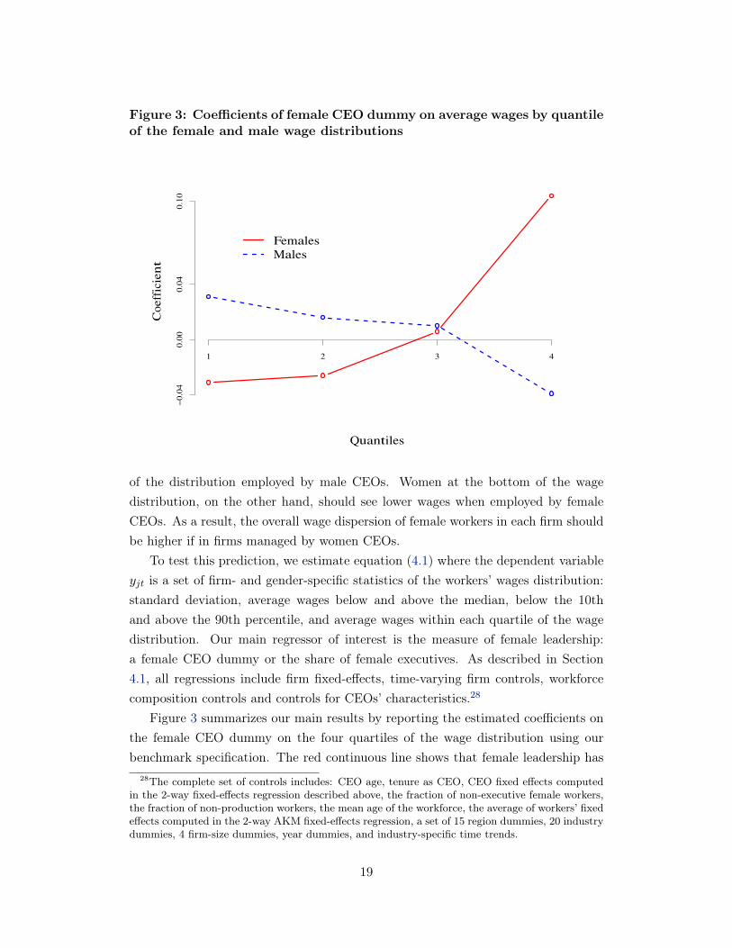
Figure 3: Coefficients of female CEO dummy on average wages by quantileof the female and male wage distributions

Quantiles

Coeffic

ient

1 2 3 4

�0.

040.

000.

040.

10

FemalesMales

of the distribution employed by male CEOs. Women at the bottom of the wagedistribution, on the other hand, should see lower wages when employed by femaleCEOs. As a result, the overall wage dispersion of female workers in each firm shouldbe higher if in firms managed by women CEOs.

To test this prediction, we estimate equation (4.1) where the dependent variableyjt is a set of firm- and gender-specific statistics of the workers’ wages distribution:standard deviation, average wages below and above the median, below the 10thand above the 90th percentile, and average wages within each quartile of the wagedistribution. Our main regressor of interest is the measure of female leadership:a female CEO dummy or the share of female executives. As described in Section4.1, all regressions include firm fixed-effects, time-varying firm controls, workforcecomposition controls and controls for CEOs’ characteristics.28

Figure 3 summarizes our main results by reporting the estimated coefficients onthe female CEO dummy on the four quartiles of the wage distribution using ourbenchmark specification. The red continuous line shows that female leadership has

28The complete set of controls includes: CEO age, tenure as CEO, CEO fixed effects computedin the 2-way fixed-effects regression described above, the fraction of non-executive female workers,the fraction of non-production workers, the mean age of the workforce, the average of workers’ fixedeffects computed in the 2-way AKM fixed-effects regression, a set of 15 region dummies, 20 industrydummies, 4 firm-size dummies, year dummies, and industry-specific time trends.

19

a positive effect on female wages at the top of distribution and a negative effect atthe bottom of the distribution. The effect on the male wage distribution is symmet-ric and of the opposite sign, as illustrated by the blue dashed line. These effects areconsistently increasing, moving from the bottom to the top of the female wage dis-tribution, whereas they are decreasing moving from the bottom to the top the maledistribution. These results conform to Empirical prediction 1 derived in Section 2.

To provide details on the precision and robustness of these results, we reportthe estimated effects of female leadership on various moments of the female wagedistribution in Table 3 and of the male wage distribution in Table 4, according to sixdifferent specifications (panels (a) through (f)).29 Coefficient estimates for the morerelevant controls are reported for the benchmark specification in the Appendix.

Panel (a) reports the results of our benchmark specification, where the measureof female leadership is a dummy variable indicating whether the firm is managed bya female CEO. This specification is estimated using the balanced sample to avoidthe selection of firms entering and exiting the sample. To eliminate possible con-founding effects induced by workers being hired or leaving after the appointment ofthe female CEO, this specification uses only observations on workers hired under theprevious CEO and who stay at the firm during the female CEO’s tenure. The otherspecifications inform the reader whether and how this sample selection and choiceof variables affect our results. The specification in panel (b) comprises all workers,including those hired by the female CEO. The specification in panel (c) includesan additional control for whether the CEO was recently appointed; this is done toaccount for the concern that the female CEO dummy might just be capturing theeffect of a CEO change. Panel (d) reports the results from the benchmark specifica-tion estimated on the full (unbalanced) panel, to check whether firm selection intothe sample plays a relevant role. Panel (e) reports results using a different measureof female leadership: the proportion of female executives.30 Finally, results in panel(f) are obtained from regressions that do not include the controls for unobservedworkforce heterogeneity and CEO ability.

For each specification, the tables report the coefficient on the measure of femaleleadership. In addition, because our model makes specific predictions on the effects

29Dependent variables in columns (4)-(9) are defined as follows: Decile 1 (column 4): averagewage of earners below the 10th percentile of the wage distribution. Decile 10 (column 5): averagewage of earners above the 90th percentile. Quantile 1: average wages below the 25th percentile;Quantile 2: average wages between the 25th and 50th percentile; Quantile 3: average wages betweenthe 50th and the 75th percentile; Quantile 4: average wages above the 75th percentile of the wagedistribution.

30Because there are more firms with at least some female executives than firms with a femaleCEO, this specification includes a larger number of firms providing a source of variation in femaleleadership compared to the other specifications.

20

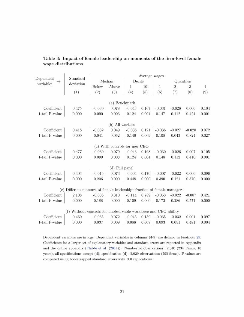
Table 3: Impact of female leadership on moments of the firm-level femalewage distributions

Dependentvariable:

! Standarddeviation

Average wagesMedian Decile Quantiles

Below Above 1 10 1 2 3 4(1) (2) (3) (4) (5) (6) (7) (8) (9)

(a) BenchmarkCoefficient 0.475 -0.030 0.078 -0.043 0.167 -0.031 -0.026 0.006 0.104

1-tail P-value 0.000 0.090 0.003 0.124 0.004 0.147 0.112 0.424 0.001

(b) All workersCoefficient 0.418 -0.032 0.049 -0.038 0.121 -0.036 -0.027 -0.020 0.072

1-tail P-value 0.000 0.041 0.062 0.146 0.009 0.108 0.043 0.824 0.027

(c) With controls for new CEOCoefficient 0.477 -0.030 0.079 -0.043 0.168 -0.030 -0.026 0.007 0.105

1-tail P-value 0.000 0.090 0.003 0.124 0.004 0.148 0.112 0.410 0.001

(d) Full panelCoefficient 0.403 -0.016 0.073 -0.004 0.170 -0.007 -0.022 0.006 0.096

1-tail P-value 0.000 0.206 0.000 0.448 0.000 0.390 0.121 0.370 0.000

(e) Different measure of female leadership: fraction of female managersCoefficient 2.108 -0.036 0.310 -0.114 0.789 -0.053 -0.022 -0.007 0.421

1-tail P-value 0.000 0.188 0.000 0.109 0.000 0.172 0.286 0.571 0.000

(f) Without controls for unobservable workforce and CEO abilityCoefficient 0.460 -0.035 0.072 -0.045 0.159 -0.035 -0.032 0.001 0.097

1-tail P-value 0.000 0.037 0.009 0.086 0.007 0.093 0.051 0.481 0.004

Dependent variables are in logs. Dependent variables in columns (4-9) are defined in Footnote 29.Coefficients for a larger set of explanatory variables and standard errors are reported in Appendixand the online appendix (Flabbi et al. (2014)). Number of observations: 2,340 (234 Firms, 10years), all specifications except (d); specification (d): 5,029 observations (795 firms). P-values arecomputed using bootstrapped standard errors with 300 replications.

21

Table 4: Impact of female leadership on moments of the firm-level malewage distributions

Dependentvariable:

! Standarddeviation

Average wagesMedian Decile Quantiles

Below Above 1 10 1 2 3 4(1) (2) (3) (4) (5) (6) (7) (8) (9)

(a) BenchmarkCoefficient -0.107 0.021 -0.027 0.029 -0.069 0.031 0.016 0.010 -0.039

1-tail P-value 0.130 0.118 0.188 0.091 0.116 0.047 0.193 0.667 0.148

(b) All workersCoefficient -0.113 -0.016 -0.037 -0.023 -0.071 -0.016 -0.015 -0.014 -0.047

1-tail P-value 0.095 0.894 0.080 0.919 0.078 0.901 0.870 0.183 0.076

(c) With controls for new CEOCoefficient -0.105 0.022 -0.027 0.029 -0.067 0.031 0.016 0.010 -0.039

1-tail P-value 0.133 0.115 0.194 0.090 0.120 0.046 0.188 0.670 0.153

(d) Full panelCoefficient -0.152 0.030 -0.038 0.058 -0.092 0.049 0.019 0.005 -0.054

1-tail P-value 0.021 0.002 0.069 0.000 0.035 0.000 0.038 0.630 0.049

(e) Different measure of female leadership: fraction of female managersCoefficient -0.232 0.008 -0.091 -0.024 -0.203 -0.004 0.016 0.004 -0.128

1-tail P-value 0.132 0.409 0.067 0.648 0.039 0.539 0.303 0.550 0.048

(f) Without controls for unobservable workforce and CEO abilityCoefficient -0.187 0.018 -0.043 0.023 -0.104 0.026 0.013 0.007 -0.060

1-tail P-value 0.013 0.154 0.059 0.148 0.027 0.077 0.231 0.629 0.037

Dependent variables are in logs. Dependent variables in columns (4-9) are defined in Footnote 29.Coefficients for a larger set of explanatory variables and standard errors are reported in AppendixB and in the online appendix (Flabbi et al. (2014)). Number of observations: 2,340 (234 Firms, 10years), all specifications except (d); specification (d): 5,029 observations (795 firms). P-values arecomputed using bootstrapped standard errors with 300 replications.

22

of female leadership on the wage variance, and on wages at the top and bottomof the gender-specific wage distributions, we report the p-values of 1-tailed testsof the model’s predictions.31 Specifically, we test the null hypothesis that femaleleadership has zero impact on the dependent variable against different alternativesspecified according to the predictions of the model. That is, we test against thealternative hypothesis that female leadership has a positive impact on the varianceof female wages, a positive impact at the top of the female wages distribution anda negative impact at the bottom. On the corresponding moments of the male wagedistribution, the alternative hypothesis is that the impact of female leadership hasthe opposite signs. Top and bottom are defined as above and below the median.32

The results can be summarized as follows.(i) Female leadership has a strong, economically and statistically significant pos-

itive effect on the variance of women’s wages, as predicted by the theory; the effect isrobust in all specifications (see column 1). The standard deviation of female wagesis almost 50% larger when the firm is managed by a female CEO in our benchmarkspecification, and over 40% larger in the other specifications using this measure offemale leadership. The effect on the male wage variance is also strong (between 10and 23 percent) and, as predicted by our model, consistently of the opposite sign,but less precisely estimated in most specifications. The null hypothesis that theeffect on the male wage variance is zero against the alternative that it is negativeis rejected in specifications (d), and (f) with p-values below 5%, and in the otherspecifications with p-values close to 10%.

(ii) The effect of female leadership on wages at top of the female wage distribution(columns 3, 5, and 9) is strongly positive and statistically significant, with p-valuesof less than 1%. For example, in our benchmark specification females with wagesabove the median earn on average 7.8% more when working for a female CEO thanfor male CEOs (Table 3 panel (a), column (3)). The effect of female leaderships isstronger at the right end of the wage distribution: the (highly significant) positiveimpact of female leadership is 10.4% for females with wages above the 25th percentile(column 9) and 16.7% for those earning above the 10th percentile. These results are

31Given that individual CEO effects are generated regressors from a first stage estimation, inall specifications except (f), P-values are computed using bootstrapped standard errors with 300replications. As described in detail in the Appendix, our bootstrapping procedure resamples firms,stratifying by firms that never had a female CEO and firms that had a female CEO. In specification(f), standard errors are clustered at the firm level. Standard errors are reported in the Appendixfor the benchmark specification and in the Web Appendix for the other specifications.

32Note that the theory predicts that the effects of female leadership should be positive or negativeat the top or bottom but does not predict non-parametrically where the change of sign should occur.Therefore, choosing the median is arbitrary. This is the reason why we add other possible cuts tothe wage distribution: top and bottom 10% and quartiles.

23

consistent across specifications. Symmetrically, the effect of female leadership onwages at the bottom of the male wage distribution (Table 4, columns 2, 4, 6, and 7)is positive and significant in most specifications.

(iii) The effect of female leadership is monotonically increasing moving from thebottom to the top of the female wage distribution (compare the estimates of columns2 and 3, 4 and 5, and of columns 6 through 9). The opposite holds true for the effecton male wages. For the benchmark specification, this is illustrated in Figure 3.

(iv) The effect of female leadership at the bottom of the female wage distribution(columns (2), (4), and (6)) is consistently negative and economically large across allspecifications, although it is less precisely estimated than the effects at the top ofthe wage distribution. For example, most specifications reject the null hypothesisthat the coefficient on the bottom half of the wage distribution is zero against thealternative that it is negative with less than 9% confidence. Specifications (b) and(f) reject the null with a p-value below 5%. Symmetrically, the estimated effects onmale wages at the top of the male distribution are consistently negative, but in thiscase they are estimated with lower precision.

(v) The estimates on the third quantile of the wage distribution (column 8 inboth tables) generally do not reject the hypothesis that the coefficients are zero.This is again consistent with the theory, which predicts that the effects of femaleleadership should be zero somewhere in the interior of the wage distribution, butdoes not predict non-parametrically where the change of sign should occur.

To summarize, the signs of our point estimates of the effects of female leadershipcorrespond to the prediction of our theoretical model. These effects are strong androbust across specifications. They are also strongly statistically significant whenpredicted to be positive. When they are predicted to be negative, the estimates thatwe obtain are close and often below conventional levels of statistical significance.

Despite the lack of strong statistical significance at the bottom in some specifi-cations, there are at least four factors that we believe work in favor of not rejectingthe theory. First, the sign of the point estimates is consistent across specifications.In particular, results are robust to extending the data to include the full panel offirms, and to including all workers (not just those that were employed at the timethe female CEO took charge of the firm). They are also not affected by excludingthe generated regressors computed in the two-way fixed-effects regression. In thiscase, the point estimates are more precisely estimated even though the reportedstandard errors are clustered at the firm level. The second factor that works in favorof not rejecting the model is that the effects are generally stronger at the extremesof the distribution, as one can observe comparing the extreme deciles to the first

24

and fourth quartiles. Third, the effects are increasing from the left to the right ofthe female wage distribution, consistent with theory. The opposite occurs on themale wage distribution. Finally, downward wage rigidity works against finding largenegative effects, especially at the bottom of the wage distribution, therefore it is notsurprising that the estimates are more precise when the effects are positive.

4.3 Female Leadership and Firm-Level Performance

In this section, we test Empirical Implication 2 from our model. Female executivesimprove the allocation of female talents within the firm by counteracting pre-existingstatistical discrimination from male executives. Therefore, we expect the efficiency-enhancing effects of female leadership to be stronger the larger the presence of femaleworkers.

Table 5 presents the estimation results from firm performance regressions, i.e.coefficients from estimating equation (4.1) where the dependent variable yjt is oneof the three measures of firm performance: sales per employee, value added peremployee, and TFP.33 The female leadership measures and the controls are the sameas those used in the wage regressions. As in the previous subsection, our benchmarkspecification focuses on the balanced panel of firms that were continuously observedfrom 1988 through 1997 (panel (a) in the table). Panel (b) reports the resultsfrom the benchmark specification run on the full (unbalanced) panel. Panel (c)reports results using the proportion of women executives as a measure of femaleleadership, and panel (d) is obtained from regressions that do not include the controlsfor unobserved workforce heterogeneity and CEO ability. In Table 5 we report thecoefficients only on the variables of interest for our results. The Appendix reportsthe set of estimated coefficients for the main explanatory variables.

Columns 1, 3, and 5 present specifications without interacting the female lead-ership dummy with the share of females in the firm’s workforce, and confirm resultsfrom the literature: as found by Wolfers (2006) and Albanesi and Olivetti (2009),34

female CEOs do not have a significant impact on firm performance.35

However, a change in the specification motivated by our model leads to differentresults. Columns 2, 4, and 6 of Table 5 report the estimates from specifications

33We computed TFP using the Olley and Pakes (1996). See Iranzo et al. (2008) for details.34Recent work on the impact of gender quotas for firms’ boards have found a negative impact

on short-term profits (Ahern and Dittmar (2012), Matsa and Miller (2013)). However, first, thesepapers consider the composition of boards, not executive bodies; second, it is not clear whetherthe impact is due to imposing a constraint on the composition of the board or to the fact that theadded members of the boards are female.

35The only exception is TFP reporting a marginally significant negative impact.

25

Table 5: Impacts of female leadership on firm-level performance

Dependentvariable:

! Sales peremployee

Value addedper employee

TFP

(1) (2) (3) (4) (5) (6)

(a) BenchmarkFemale leadership 0.033 -0.120 -0.046 -0.245 -0.059 -0.213Std. Error (0.039) (0.045) (0.038) (0.041) (0.029) (0.039)Interaction 0.610 0.795 0.6161-tail P-value 0.000 0.000 0.000

(b) Full PanelFemale leadership 0.029 -0.009 -0.049 -0.093 -0.061 -0.096Std. Error (0.024) (0.034) (0.026) (0.032) (0.024) (0.031)Interaction 0.123 0.144 0.1151-tail P-value 0.066 0.022 0.041

(c) Alternative measure of leadership: fraction of female execs.Female leadership 0.033 -0.120 -0.046 -0.245 -0.059 -0.213Std. Error (0.039) (0.045) (0.038) (0.041) (0.029) (0.039)Interaction 0.610 0.795 0.6161-tail P-value 0.000 0.000 0.000

(d) Without controls for unobservable workforce and CEO abilityFemale leadership 0.027 -0.104 -0.064 -0.234 -0.072 -0.200Std. Error (0.061) (0.071) (0.058) (0.057) (0.045) (0.051)Interaction 0.523 0.677 0.5131-tail P-value 0.001 0.000 0.002

Female leadership: Female CEO dummy (panels a, b, and c); Fraction of female executives (panelc); Interaction: female leadership interacted with the fraction of female workers (non-executive).Coefficients for a larger set of explanatory variables and standard errors are reported in AppendixB and in the online appendix (Flabbi et al. (2014)).

where the measure of female leadership is interacted with the proportion of non-executive female workers in the firm.36 As predicted by theory, we find a positiveand significant coefficient on this interaction variable for each of the three measuresof firm performance. The magnitude of the impact is substantial: for example,based on our benchmark estimates (column (2) in panel (a) of Table 5), a female

36Just as in the wage regressions, we only focus on non-executives because the theory presentedin Section 2 is not modeling promotion to executive, executive pay or interaction within executives.

26

Table 6: Impact of gender quotas

Counterfactual Average percent gain Percent gain for treatedCEO Allocation Quota Sales Value added TFP Sales Value added TFPFemale share > 20% 51% 6.7 4.2 2.1 14.2 8.7 4.3Random 51% 1.9 -2.1 -2.7 3.7 -4.1 -5.4

Note: average percent gains relative to fitted data. “Treated” firms are firms that acquire a femaleCEO.

CEO taking over a firm employing the average proportion of women in the samplewould increase sales per employee by about 3.2%; if half of the firm’s workers werewomen the impact would be about 18.5%.

The results are robust to using the full, unbalanced, sample (panel (b)), to adopt-ing an alternative measure of female leadership (panel (c)), and to changing thespecification to avoid using generated regressors (panel (d)). Overall, these resultsconfirm Empirical prediction 2 derived from the theory.

4.4 Potential efficiency gains from gender quotas

In order to provide an order of magnitude of the potential efficiency gains generatedby increasing the presence of women in corporate leadership positions, for examplethrough gender quotas, we consider a partial-equilibrium exercise using the param-eter estimates from our benchmark specification reported in Table 5. We performedtwo counterfactuals. One is a “targeted” exercise where we allocated a female CEOto all firms whose performance would improve as a result, that is, firms with at least20 percent of female employees. This results in 51% of firms with a woman CEO. Inthe other exercise, we assign a female CEO to the same proportion of firms (51%)selected randomly. Results are in Table 6.

When Female CEOs are allocated randomly, the average percent change is gen-erally small, and its sign depends on the measure of performance. In contrast, our“targeted” exercise delivers large, positive effects in the firms that are assigned a fe-male CEO, and also positive effects overall. For example, the table shows that in thisscenario sales per worker would increase by 14.2% in the “treated” firms (firms whoseCEO’s gender has changed) and by 6.7% in the overall sample of firms. This is be-cause our findings imply large, positive interaction effects between female leadershipand the share of female workers. Although our exercises ignore general equilibriumeffects, these results confirm that, based on our estimates, the order of magnitude

27

of the efficiency gains from having a larger female representation in firm leadershipcan be quite large.37

5 Other Explanations

5.1 Gender Preferences

A possible alternative explanation for our results is that female CEOs give preferen-tial treatment to female workers. However, such an explanation is at odds with atlest two of our findings. First, the effect of female leadership on female wages varieswith the wage level, so much so that the impact at lower wages is negative. A theorybased on preferences would require the ad-hoc assumption that the CEOs preferencesfor women are conditional on their wage level. In particular, a female CEO wouldneed to prefer female workers at the top of the distribution, and to hold prejudiceagainst women at the bottom of the distribution. Second, preferential treatment isinconsistent with our results on firm performance illustrated in Subsection 4.3. Iffemale CEOs gave preferential treatment to female workers, they would be proneto hire and promote female workers even if males with identical characteristics weremore productive. As a result, the impact on performance of the interaction betweenfemale leadership and share of females would unlikely be positive.38

5.2 Complementarities Between Female Managers and SkilledFemale Workers

Complementarities between female managers and skilled labor input from femaleworkers may be consistent with some of our results depending on the source of suchcomplementarities. For example, one could assume that communication is more ef-ficient between workers and executives of the same gender. This communicationtechnology is not in contradiction with our model. In fact, it provides a possiblemicro-foundation for the crucial assumption of our statistical discrimination frame-work: the difference in the quality of signals from workers of different gender.

However, similar effects could be also derived from a complete information modelwhere communication skills enter directly into the production function. For example,

37The effect on the average gender wage gap, not shown in the table, is small. In firms acquir-ing female leadership, the higher wages of female workers at the high end of the distribution arecompensated by lower wages at the low end of the wage distribution.

38Bednar and Gicheva (2014) find support for a similar conclusion. Using a matched manager-firm data with information about the gender composition in lower levels of the job ladder, and theydo not find evidence that gender is predictive of a supervisor’s female-friendliness.

28

complementarities may be generated by peer-group effects or because female man-agers are role models for skilled female workers.39 These explanations can indeedgenerate the productivity effects we find in our results. They can also generate oneresult from the wage regressions: the positive effect of female leadership on femalewages at the top of the distribution. However, these alternative explanations areunable to generate the two other results we obtain from the wage regressions: thenegative effect of female leadership on female wages at the bottom of the distribu-tion, and any effect of female leadership on the male wage distribution. We concludethat the balance of the evidence favors our statistical discrimination model.

6 Conclusion

Motivated by a recent literature showing the importance of executives’ personaltraits in determining firm policies and outcomes, and by the traditional literatureon gender differentials in the labor market, we investigate whether female executivesmake a difference on gender-specific wage distributions and on firm performance. Wefind that female CEOs increase the variance of women’s wages at the firm becausethey have a positive impact on wages at the top of the distribution, and a (smaller)negative impact on wages at the bottom. In our preferred specification, female CEOsincrease wages for women in the top 25% of the women’s wage distribution by about10 percentage points and they decrease wages for women in the bottom 25% by about3 percentage points. The impact on the men’s wage distribution has opposite signs.Our results are robust to alternative measures of female leadership, to different em-pirical specifications and to different sample selection criteria for firms and workers.When looking at the impact on firm performance, we estimate that the interactionbetween female CEOs and the share of female workers employed at the firm hasa positive impact on firm performance. The magnitude of the impact is substan-tial: in our preferred specification, a female CEO taking over a male-managed firmwith at least 20% women in the workforce increases sales per employee by about14%. The results are robust to three different measures of firm productivity, onedifferent measure of female leadership, and two different specifications and estima-tion samples. Moreover, we exploited the matched employer-employee, longitudinalstructure of our data to construct a rich set of controls for firm-level, workforce-level,and executive-level heterogeneity, thereby alleviating selection bias concerns.

This evidence is consistent with a model of statistical discrimination where femaleexecutives are better equipped at interpreting signals of productivity from female

39Athey et al. (2000) introduce a model analyzing the effects of mentoring on workplace diversity.

29

workers. As a result of this attenuated information asymmetry, female CEOs takingcharge of previously male-led firms are able to reverse statistical discrimination,paying women wages that are closer to their actual productivity and matching themto jobs that are more in line with their skills.

Interpreting our results through the implications of our theoretical model suggeststhat there are potentially high costs associated with the under-representation ofwomen at the top of corporate hierarchies. Companies with a substantial femalepresence would be likely to benefit from assigning women to leadership positions.Results from a partial-equilibrium counterfactual experiment based on our pointestimates show if all the firms with at least 20% of female workers were lead by femaleCEOs, they would see their sales per worker increase by about 14.2%. From a publicpolicy point of view, the same partial-equilibrium counterfactual experiment showsthat an integrated generalized extension of women in leadership positions would leadto a much smaller,40 but still positive effect on sales per worker.

A Appendix: Proof of Proposition 1

Proof. Define bs as the signal such that the wage of male and females is the same.From (2.2) note that bs is independent of the task assignment, and satisfies �m(q|bs) =�f (q|bs); bs exists and is unique because the cumulatives of two Normal distributionswith different variance cross only once.41 Under the assumption �✏f > �✏m, �m hasthinner tails than �f , therefore:

1� 2�m(q|s) < 1� 2�f (q|s) for all s < bs (A.1)

1� 2�f (q|s) < 1� 2�m(q|s) for all s > bs (A.2)

Observe also from (2.2) that either bs min{sm, sf}, or bs � max{sm, sf}. Toprove it, note that by definition of sg, �m(q|sm) = �f (q|sf ) = 1/2, therefore ifsm < sf we must have �f (q|s) < 1/2 < �m(q|s), for all s 2 (sm, sf ); other-wise, if sm > sf we must have �m(q|s) < 1/2 < �f (q|s) for all s 2 (sf , sm).

403.7% instead of 14.2%, see Table 6. Results on Value Added and TFP would actually turn frompositive to negative, with magnitudes always smaller than in the sales per worker case.

41Consider two normal distributions F,G with different variance (�F > �G). Then, regardlesstheir mean, there exists a unique x : F (x) > G(x) for all x < x, and F (x) < G(x) for all x > x.To prove this single crossing property, denote with f, g the densities of distributions F,G. Becausef, g are symmetric around their respective means, and �F > �G, the two densities intersect atpoints x1, x2 with f(x) > g(x) if x < x1 or x < x2, and f(x) < g(x) for x1 < x < x2. But thenF (x) > G(x) for all x < x1 and 1 � F (x) > 1 � G(x), or F (x) < G(x) for x > x2. Hence anyintersection between F and G must occur between x1 and x2, but in this range f(x) > g(x), that is,F (x) has derivative greater than the derivative of G(x), therefore there can be only one intersection.

30

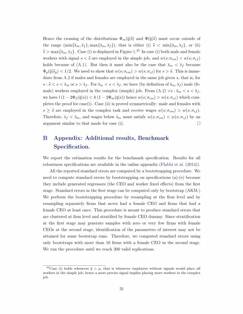
Hence the crossing of the distributions �m(q|bs) and �(q|bs) must occur outside ofthe range (min{sm, sf},max{sm, sf}), that is either (i) bs < min{sm, sf}, or (ii)bs > max{sm, sf}. Case (i) is displayed in Figure 1.42 In case (i) both male and femaleworkers with signal s < bs are employed in the simple job, and w(s;�✏m) < w(s;�✏f )

holds because of (A.1). But then it must also be the case that sm < sf because�g(q|bsg) < 1/2. We need to show that w(s;�✏m) > w(s;�✏f ) for s > bs. This is imme-diate from A.2 if males and females are employed in the same job given s, that is, fors : bs < s < sm or s > sf . For sm < s < sf , we have (by definition of sm, sf ) male (fe-male) workers employed in the complex (simple) job. From (A.2) _s : sm < s < sf ,we have l (1� 2�f (q|s)) < h (1� 2�m(q|s)) hence w(s;�✏m) > w(s;�✏f ) which com-pletes the proof for case(i). Case (ii) is proved symmetrically: male and females withs � bs are employed in the complex task and receive wages w(s;�✏m) > w(s;�✏f ).Therefore, sf < sm, and wages below sm must satisfy w(s;�✏m) < w(s;�✏f ) by anargument similar to that made for case (i).

B Appendix: Additional results, BenchmarkSpecification.

We report the estimation results for the benchmark specification. Results for allrobustness specifications are available in the online appendix (Flabbi et al. (2014)).

All the reported standard errors are computed by a bootstrapping procedure. Weneed to compute standard errors by bootstrapping on specifications (a)-(e) becausethey include generated regressors (the CEO and worker fixed effects) from the firststage. Standard errors in the first stage can be computed only by bootstrap (AKM.)We perform the bootstrapping procedure by resampling at the firm level and byresampling separately firms that never had a female CEO and firms that had afemale CEO at least once. This procedure is meant to produce standard errors thatare clustered at firm level and stratified by female CEO dummy. Since stratificationat the first stage may generate samples with zero or very few firms with femaleCEOs at the second stage, identification of the parameters of interest may not beattained for some bootstrap runs. Therefore, we computed standard errors usingonly bootstraps with more than 10 firms with a female CEO in the second stage.We run the procedure until we reach 300 valid replications.

42Case (i) holds whenever q > µ, that is whenever employers without signals would place allworkers in the simple job, hence a more precise signal implies placing more workers in the complexjob.

31

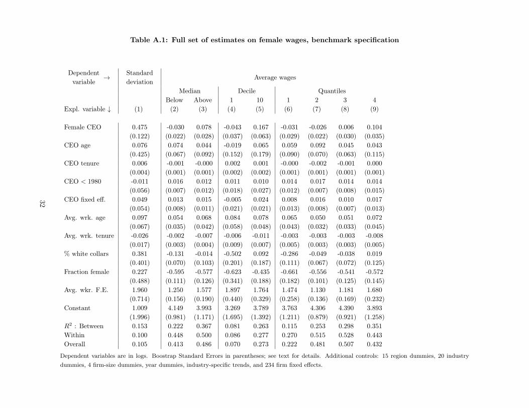
Table A.1: Full set of estimates on female wages, benchmark specification

Dependentvariable

! Standarddeviation

Average wages

Median Decile QuantilesBelow Above 1 10 1 2 3 4

Expl. variable # (1) (2) (3) (4) (5) (6) (7) (8) (9)

Female CEO 0.475 -0.030 0.078 -0.043 0.167 -0.031 -0.026 0.006 0.104(0.122) (0.022) (0.028) (0.037) (0.063) (0.029) (0.022) (0.030) (0.035)

CEO age 0.076 0.074 0.044 -0.019 0.065 0.059 0.092 0.045 0.043(0.425) (0.067) (0.092) (0.152) (0.179) (0.090) (0.070) (0.063) (0.115)

CEO tenure 0.006 -0.001 -0.000 0.002 0.001 -0.000 -0.002 -0.001 0.000(0.004) (0.001) (0.001) (0.002) (0.002) (0.001) (0.001) (0.001) (0.001)

CEO < 1980 -0.011 0.016 0.012 0.011 0.010 0.014 0.017 0.014 0.014(0.056) (0.007) (0.012) (0.018) (0.027) (0.012) (0.007) (0.008) (0.015)

CEO fixed eff. 0.049 0.013 0.015 -0.005 0.024 0.008 0.016 0.010 0.017(0.054) (0.008) (0.011) (0.021) (0.021) (0.013) (0.008) (0.007) (0.013)

Avg. wrk. age 0.097 0.054 0.068 0.084 0.078 0.065 0.050 0.051 0.072(0.067) (0.035) (0.042) (0.058) (0.048) (0.043) (0.032) (0.033) (0.045)

Avg. wrk. tenure -0.026 -0.002 -0.007 -0.006 -0.011 -0.003 -0.003 -0.003 -0.008(0.017) (0.003) (0.004) (0.009) (0.007) (0.005) (0.003) (0.003) (0.005)

% white collars 0.381 -0.131 -0.014 -0.502 0.092 -0.286 -0.049 -0.038 0.019(0.401) (0.070) (0.103) (0.201) (0.187) (0.111) (0.067) (0.072) (0.125)

Fraction female 0.227 -0.595 -0.577 -0.623 -0.435 -0.661 -0.556 -0.541 -0.572(0.488) (0.111) (0.126) (0.341) (0.188) (0.182) (0.101) (0.125) (0.145)

Avg. wkr. F.E. 1.960 1.250 1.577 1.897 1.764 1.474 1.130 1.181 1.680(0.714) (0.156) (0.190) (0.440) (0.329) (0.258) (0.136) (0.169) (0.232)

Constant 1.009 4.149 3.993 3.269 3.789 3.763 4.306 4.390 3.893(1.996) (0.981) (1.171) (1.695) (1.392) (1.211) (0.879) (0.921) (1.258)

R2 : Between 0.153 0.222 0.367 0.081 0.263 0.115 0.253 0.298 0.351Within 0.100 0.448 0.500 0.086 0.277 0.270 0.515 0.528 0.443Overall 0.105 0.413 0.486 0.070 0.273 0.222 0.481 0.507 0.432

Dependent variables are in logs. Boostrap Standard Errors in parentheses; see text for details. Additional controls: 15 region dummies, 20 industrydummies, 4 firm-size dummies, year dummies, industry-specific trends, and 234 firm fixed effects.

32

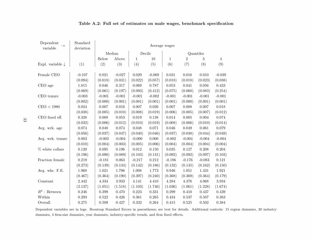
Table A.2: Full set of estimates on male wages, benchmark specification

Dependentvariable

! Standarddeviation

Average wages

Median Decile QuantilesBelow Above 1 10 1 2 3 4

Expl. variable # (1) (2) (3) (4) (5) (6) (7) (8) (9)

Female CEO -0.107 0.021 -0.027 0.029 -0.069 0.031 0.016 0.010 -0.039(0.094) (0.018) (0.031) (0.022) (0.057) (0.018) (0.018) (0.023) (0.038)

CEO age 1.815 0.046 0.317 0.069 0.787 0.053 0.041 0.056 0.433(0.869) (0.061) (0.197) (0.093) (0.412) (0.075) (0.060) (0.083) (0.254)

CEO tenure -0.003 -0.001 -0.001 -0.001 -0.002 -0.001 -0.001 -0.001 -0.001(0.002) (0.000) (0.001) (0.001) (0.001) (0.001) (0.000) (0.001) (0.001)

CEO < 1980 0.024 0.007 0.016 0.007 0.026 0.007 0.008 0.007 0.018(0.038) (0.005) (0.010) (0.008) (0.019) (0.006) (0.005) (0.007) (0.012)

CEO fixed eff. 0.328 0.008 0.053 0.019 0.138 0.014 0.005 0.004 0.074(0.032) (0.006) (0.012) (0.010) (0.019) (0.008) (0.006) (0.010) (0.014)

Avg. wrk. age 0.074 0.048 0.074 0.048 0.071 0.046 0.049 0.061 0.079(0.056) (0.037) (0.047) (0.040) (0.046) (0.037) (0.038) (0.044) (0.049)

Avg. wrk. tenure 0.003 -0.003 -0.004 -0.000 0.000 -0.002 -0.004 -0.004 -0.004(0.010) (0.004) (0.003) (0.005) (0.006) (0.004) (0.004) (0.004) (0.004)

% white collars 0.120 0.095 0.196 0.012 0.150 0.035 0.127 0.208 0.204(0.196) (0.090) (0.089) (0.103) (0.131) (0.092) (0.092) (0.097) (0.103)

Fraction female 0.219 -0.181 0.063 -0.217 0.212 -0.186 -0.176 -0.083 0.121(0.273) (0.139) (0.134) (0.142) (0.186) (0.132) (0.145) (0.162) (0.150)

Avg. wkr. F.E. 1.968 1.021 1.796 1.008 1.773 0.946 1.051 1.431 1.921(0.467) (0.364) (0.190) (0.397) (0.240) (0.368) (0.369) (0.364) (0.179)

Constant 2.442 4.334 3.933 4.141 4.410 4.284 4.376 4.068 3.934(2.137) (1.051) (1.518) (1.103) (1.746) (1.036) (1.061) (1.228) (1.674)

R2 : Between 0.246 0.399 0.470 0.223 0.331 0.299 0.410 0.437 0.439Within 0.293 0.522 0.426 0.361 0.265 0.434 0.537 0.507 0.383Overall 0.275 0.509 0.427 0.332 0.264 0.415 0.525 0.502 0.384

Dependent variables are in logs. Boostrap Standard Errors in parentheses; see text for details. Additional controls: 15 region dummies, 20 industrydummies, 4 firm-size dummies, year dummies, industry-specific trends, and firm fixed effects.

33

Table A.3: Estimates on Firm-Level Performance, benchmark specification

Dependentvariable

! Sales peremployee

Value addedper employee

TFP

. variable # (1) (2) (3) (4) (5) (6)

Female CEO 0.033 -0.120 -0.046 -0.245 -0.059 -0.213(0.039) (0.045) (0.038) (0.041) (0.029) (0.039)

Interaction 0.610 0.795 0.616(0.142) (0.169) (0.172)

CEO age 0.212 0.209 0.442 0.438 0.320 0.316(0.154) (0.152) (0.162) (0.160) (0.146) (0.145)

CEO tenure -0.003 -0.003 -0.002 -0.002 -0.002 -0.001(0.001) (0.001) (0.001) (0.001) (0.001) (0.001)

CEO started <1980 0.028 0.028 0.012 0.011 0.010 0.010(0.014) (0.014) (0.015) (0.015) (0.015) (0.015)

CEO fixed eff. 0.017 0.017 0.065 0.064 0.046 0.045(0.019) (0.018) (0.017) (0.017) (0.017) (0.017)

Avg. Wkr. age 0.028 0.031 0.051 0.055 0.055 0.058(0.027) (0.028) (0.031) (0.033) (0.029) (0.029)

Avg wkr. tenure 0.005 0.004 -0.013 -0.014 -0.030 -0.030(0.008) (0.008) (0.007) (0.007) (0.007) (0.007)

% white collars 0.269 0.254 -0.117 -0.137 -0.082 -0.098(0.135) (0.136) (0.154) (0.155) (0.154) (0.154)

Fraction female -0.313 -0.390 -0.496 -0.596 -0.478 -0.556(0.234) (0.242) (0.157) (0.158) (0.164) (0.161)

Avg. wkr. F.E. 1.217 1.284 1.636 1.724 1.438 1.506(0.267) (0.264) (0.299) (0.305) (0.305) (0.299)

Constant 3.089 3.020 2.072 1.983 0.422 0.353(0.640) (0.653) (0.830) (0.868) (0.697) (0.708)

R2: Between 0.590 0.592 0.218 0.222 0.179 0.182Within 0.013 0.015 0.044 0.055 0.270 0.268Overall 0.070 0.073 0.070 0.081 0.248 0.247

Dependent variables are in logs. Boostrap Standard Errors in parentheses; see text for details.Additional controls: 15 region dummies, 20 industry dummies, 4 firm-size dummies, year dummies,industry-specific trends, and firm fixed effects.

34

References

Abowd, John M., Francis Kramarz, and David N Margolis, “High wageworkers and high wage firms,” Econometrica, 1999, 67 (2), 251–333.

, Robert H. Creecy, and Francis Kramarz, “Computing person and firmeffects using linked longitudinal employer-employee data,” Center for EconomicStudies, US Census Bureau, 2002, (2002-06).

Adams, Renee B and Daniel Ferreira, “Women in the boardroom and theirimpact on governance and performance,” Journal of Financial Economics, 2009,94 (2), 291–309.

Ahern, Kenneth R and Amy K Dittmar, “The changing of the boards: Theimpact on firm valuation of mandated female board representation,” The QuarterlyJournal of Economics, 2012, 127 (1), 137–197.

Albanesi, Stefania and Claudia Olivetti, “Home production, market produc-tion and the gender wage gap: Incentives and expectations,” Review of Economicdynamics, 2009, 12 (1), 80–107.

Albrecht, James, Anders Björklund, and Susan Vroman, “Is there a glassceiling in Sweden?,” Journal of Labor Economics, 2003, 21 (1), 145–177.

Angier, M. and B. Axelrod, “Realizing the Power of Talented Women,” McKinseyQuarterly, 2014, 3 (107-115).

Athey, Susan, Christopher Avery, and Peter Zemsky, “Mentoring and diver-sity,” American Economic Review, September 2000, 90 (4), 765–786.

Bagues, Manuel and Maria J. Perez-Villadoniga, “Why Do I Like People LikeMe?,” Journal of Economic Theory, May 2013, 148 (3), 1292–9.

Bandiera, Oriana, Andrea Prat, Luigi Guiso, and Raffaella Sadun, “Match-ing firms, managers and incentives,” National Bureau of Economic Research Work-ing Paper, 2011, (16691).

Bednar, Steven and Dora Gicheva, “Are Female Supervisors More Female-Friendly?,” The American Economic Review, 2014, 104 (5), 370–375.

Bell, Linda A, “Women-led firms and the gender gap in top executive jobs,” IZADiscussion Papers, 2005.

35

Bennedsen, Morten, F Perez-Gonzales, and Daniel Wolfenzon, “Evaluatingthe Impact of The Boss: Evidence from CEO Hospitalization Events,” UnpublishedManuscript, 2012.

Bertrand, Marianne and Antoinette Schoar, “Managing with Style: the Effectof Managers on Firm Policies,” The Quarterly Journal of Economics, 2003, 118(4), 1169–1208.

and Kevin F. Hallock, “The Gender gap in top corporate jobs,” Industrial andLabor Relations Review, October 2001, 55 (1), 3–21.

, S Black, Sissel Jensen, and Adriana Lleras-Muney, “Breaking the GlassCeiling? The Effect of Board Quotas on Female Labor Market Outcomes in Nor-way,” Unpublished Manuscript, 2014.

Blau, Francine D and Lawrence M Kahn, “The US gender pay gap in the 1990s:Slowing convergence,” NBER Working Papers, 2004.

Bloom, Nicholas and John Van Reenen, “Measuring and explaining manage-ment practices across firms and countries,” The Quarterly Journal of Economics,2007, 122 (4), 1351–1408.

and , “Why do management practices differ across firms and countries?,” TheJournal of Economic Perspectives, 2010, 24 (1), 203–224.

Card, David, Jörg Heining, and Patrick Kline, “Workplace Heterogeneity andthe Rise of West German Wage Inequality,” The Quarterly Journal of Economics,August 2013, 128, 967–1015.

Cardoso, Ana Rute and Rudolf Winter-Ebmer, “Female-Led Firms and Gen-der Wage Policies,” Industrial and Labor Relations Review, 2010, 61 (1), 143–63.

Cooper-Patrick, Lisa, Joseph J Gallo, Junius J Gonzales, Hong Thi Vu,Neil R Powe, Christine Nelson, and Daniel E Ford, “Race, gender, andpartnership in the patient-physician relationship,” Jama, 1999, 282 (6), 583–589.

Cornell, Bradford and Ivo Welch, “Culture, information, and screening discrim-ination,” Journal of Political Economy, 1996, pp. 542–571.

Dezsö, Cristian L and David Gaddis Ross, “Does female representation in topmanagement improve firm performance? A panel data investigation,” StrategicManagement Journal, 2012, 33 (9), 1072–1089.

36

Dindia, Kathryn and Daniel J Canary, Sex differences and similarities in com-munication, Psychology Press, 2006.

Eaton, Morris L., Multivariate Statistics : A Vector Space Approach Wiley seriesin probability and mathematical statistics, New York : Wiley, 1983.

Eckstein, Zvi and Eva Nagypal, “The evolution of US earnings inequality: 1961-2002,” Federal Reserve Bank of Minneapolis Quarterly Review, 2004, 28 (2), 10–29.

Ellison, Sara Fisher and Wallace P Mullin, “Diversity, Social Goods Provision,and Performance in the Firm,” Journal of Economics & Management Strategy,2014, 23 (2), 465–481.

Fadlon, Yariv, “Essays on Statistical Discrimination and on the Payoff to Publish-ing in Economics Journals.” PhD dissertation, Vanderbilt University 2010.

Fang, Hanming and Andrea Moro, “Theories of Statistical Discrimination andAffirmative Action: A Survey,” in Jess Benhabib, Matthew O. Jackson, and Al-berto Bisin, eds., Handbook of Social Economics, Volume 1A, Vol. 1A, The Nether-lands: North Holland, 2011, chapter V, pp. 133–200.

Farrell, Kathleen A and Philip L Hersch, “Additions to corporate boards: theeffect of gender,” Journal of Corporate Finance, 2005, 11 (1), 85–106.

Flabbi, Luca, “Prejudice and gender differentials in the US labor market in the lasttwenty years,” Journal of Econometrics, 2010, 156 (1), 190–200.

, Mario Macis, Andrea Moro, and Fabiano Schivardi, “Do Female Execu-tives Make a Difference? The Impact of Female Leadership on Gender Gaps andFirm Performance. External Appendix.,” Unpublished Manuscript, 2014. (down-load link).

Gabaix, Xavier and Augustin Landier, “Why has CEO pay increased so much?,”The Quarterly Journal of Economics, 2008, 123 (1), 49–100.

Gagliarducci, Stefano and M. Daniele Paserman, “Gender Interactions inFirm Hierarchies: Evidence from Linked Employer-Employee Data,” UnpublishedManuscript, March 2014.

Gayle, George-Levi, Limor Golan, and Robert A Miller, “Gender Differencesin Executive Compensation and Job Mobility,” Journal of Labor Economics, 2012,30 (4), 829–872.

37

Iranzo, Susana, Fabiano Schivardi, and Elisa Tosetti, “Skill Dispersion andFirm Productivity: An Analysis with Employer-Employee Matched Data,” Journalof Labor Economics, 2008, 26 (2), 247–285.

Kaplan, Steven N, Mark M Klebanov, and Morten Sorensen, “Which CEOcharacteristics and abilities matter?,” The Journal of Finance, 2012, 67 (3), 973–1007.

Lang, Kevin, “A language theory of discrimination,” The Quarterly Journal ofEconomics, 1986, pp. 363–382.

Lazear, Edward P, Kathryn L Shaw, and Christopher T Stanton, “TheValue of Bosses,” National Bureau of Economic Research Working Paper, 2012,(18317).

Lippi, Francesco and Fabiano Schivardi, “Corporate control and executive se-lection,” Quantitative Economics, 2014, 5 (2), 417–456.

Malmendier, Ulrike and Geoffrey Tate, “CEO overconfidence and corporateinvestment,” The Journal of Finance, 2005, 60 (6), 2661–2700.

Mast, Marianne Schmid, Judith A Hall, and Debra L Roter, “Disentanglingphysician sex and physician communication style: their effects on patient satis-faction in a virtual medical visit,” Patient education and counseling, 2007, 68 (1),16–22.

Matsa, David A. and Amalia R. Miller, “A Female Style in Corporate Leader-ship? Evidence from Quotas,” American Economic Journal: Applied Economics,2013, 5 (3), 136–69.

Morgan, John and Felix Várdy, “Diversity in the Workplace,” The AmericanEconomic Review, 2009, pp. 472–485.

Olley, G Steven and Ariel Pakes, “The Dynamics of Productivity in the Telecom-munica# tions Equipment Industry, mEconometrica 64,” Econometrica, 1996, 64,1263–1297.

Phelps, Edmund S, “The Statistical Theory of Racism and Sexism,” The AmericanEconomic Review, 1972, 62 (4), 659–661.

Rathore, Saif S, Jersey Chen, Yongfei Wang, Martha J Radford, ViolaVaccarino, and Harlan M Krumholz, “Sex differences in cardiac catheteriza-tion: the role of physician gender,” Jama, 2001, 286 (22), 2849–2856.

38

Rose, Caspar, “Does female board representation influence firm performance? TheDanish evidence,” Corporate Governance: An International Review, 2007, 15 (2),404–413.

Scollon, Ron, Suzanne Wong Scollon, and Rodney H Jones, Interculturalcommunication: A discourse approach, John Wiley & Sons, 2011.

Smith, Nina, Valdemar Smith, and Mette Verner, “Do women in top manage-ment affect firm performance? A panel study of 2,500 Danish firms,” InternationalJournal of Productivity and Performance Management, 2006, 55 (7), 569–593.

Tervio, Marko, “The difference that CEOs make: An assignment model approach,”The American Economic Review, 2008, 98 (3), 642–668.

Wolfers, Justin, “Diagnosing discrimination: Stock returns and CEO gender,”Journal of the European Economic Association, 2006, 4 (2-3), 531–541.

39