FEDERAL RESERVE BANK OF SAN FRANCISCO

WORKING PAPER SERIES

Do Extended Unemployment Benefits Lengthen Unemployment Spells?

Evidence from Recent Cycles in the U.S. Labor Market

Henry S. Farber, Princeton University, NBER, IZA

Robert G. Valletta,

Federal Reserve Bank of San Francisco, IZA

April 2013

The views in this paper are solely the responsibility of the authors and should not be interpreted as reflecting the views of the Federal Reserve Bank of San Francisco or the Board of Governors of the Federal Reserve System.

Working Paper 2013-09 http://www.frbsf.org/publications/economics/papers/2013/wp2013-09.pdf

Version: April 8, 2013

Do Extended Unemployment Benefits Lengthen Unemployment Spells?Evidence from Recent Cycles in the U.S. Labor Market1

Henry S. Farber Robert G. Valletta

Princeton University, NBER, IZA Federal Reserve Bank of San Francisco, IZA

Abstract

In response to the Great Recession and sustained labor market downturn, the avail-

ability of unemployment insurance (UI) benefits was extended to new historical highs

in the United States, up to 99 weeks as of late 2009 into 2012. We exploit variation

in the timing and size of UI benefit extensions across states to estimate the overall

impact of these extensions on unemployment duration, comparing the experience with

the prior extension of benefits (up to 72 weeks) during the much milder downturn in

the early 2000s. Using monthly matched individual data from the U.S. Current Popu-

lation Survey (CPS) for the periods 2000-2005 and 2007-2012, we estimate the effects

of UI extensions on unemployment transitions and duration. We rely on individual

variation in benefit availability based on the duration of unemployment spells and the

length of UI benefits available in the state and month, conditional on state economic

conditions and individual characteristics. We find a small but statistically significant

reduction in the unemployment exit rate and a small increase in the expected duration

of unemployment arising from both sets of UI extensions. The effect on exits and dura-

tion is primarily due to a reduction in exits from the labor force rather than a decrease

in exits to employment (the job finding rate). The magnitude of the overall effect on

exits and duration is similar across the two episodes of benefit extensions. Although

the overall effect of UI extensions on exits from unemployment is small, it implies a

substantial effect of extended benefits on the steady-state share of unemployment in

the cross-section that is long-term.

1Farber: Industrial Relations Section, Firestone Library, Princeton University, Princeton, NJ 08544.

Phone: (609)258-4044. email: farber@princeton.edu. Valletta: Federal Reserve Bank of San Francisco, 101

Market St. San Francisco, CA 94105. Phone: (415)974-3345. email: rob.valletta@sf.frb.org. We thank

participants at numerous workshops and conferences since 2011 for their comments on various versions of

this paper. We especially thank Jesse Rothstein for detailed discussions regarding data construction and

Scott Gibbons of the U.S. Department of Labor and Julie Whittaker of the Congressional Research Service

for their assistance with obtaining and interpreting data on extended UI benefits. We also thank Katherine

Kuang and Leila Bengali for outstanding research assistance. The views expressed in this paper are solely

those of the authors and should not be attributed to the Federal Reserve Bank of San Francisco or the

Federal Reserve System.

1 Introduction

Compared with other advanced industrial countries, the United States is among the least

generous with respect to the duration and level of unemployment insurance (UI) benefits

(OECD 2007). Under normal economic circumstances, UI benefits in the United States are

available for up to six months following job loss, compared with availability of a year or longer

in many European countries. In response to the severe labor market downturn associated

with “The Great Recession” of 2007-09, however, UI benefit availability was successively

extended in the United States, reaching a maximum duration of 99 weeks as of late 2009

and continuing into 2012. This unprecedented expansion of UI availability has been the

subject of intense policy debate, which has largely revolved around the incentive effects of

UI payments on job search and prolonged labor force attachment.1 In this paper, we provide

an empirical assessment of the impact of extended UI on exit rates from unemployment and

duration of unemployment in the United States. We focus in particular on a comparison

between the effects of the recent UI extensions and those triggered by the earlier, less severe

labor market downturn in the early 2000s.

Past empirical research has produced a range of estimates regarding the disincentive

effects of UI benefits on job search in the United States (e.g., Moffitt 1985, Katz and Meyer

1990, Card and Levine 2000). However, as noted by others (e.g., Katz 2010), the impact of

UI benefits on job search likely was higher in the 1970s and 1980s than it is now, due to

the earlier period’s greater reliance on temporary layoffs and the corresponding sensitivity

of recall dates to unemployment insurance benefits. Moreover, recent research suggests that

the disincentive effects of UI are limited by the reduced returns to job search under weak

labor market conditions (e.g., Landais, Michaillat, and Saez 2010; Kroft and Notowidigdo

2011); it may be that such considerations loomed especially large during the Great Recession.

Rothstein (2011), who presents an analysis of the effects of the recent UI extensions that is

similar in approach to ours, reports small effects of the recent UI extensions on unemployment

exits, duration, and the overall unemployment rate.

Because extended UI benefits were much more widely available during the Great Re-

cession than during earlier periods and because of the severity of the recent labor market

downturn, earlier empirical results cannot be reliably extrapolated to assess UI disincentive

effects in the recent episode. We estimate these effects by developing a framework that relies

on current labor market data and detailed information on the recent UI expansions. We

1 Relevant prior research includes Chetty (2008) and Card, Chetty, and Weber (2007).

1

use microdata at the individual level from the monthly survey of households and individuals

that is used to construct official unemployment and labor force statistics in the United States

(the Current Population Survey, or CPS). We match observations on individuals across con-

secutive months of the data, which enables us to analyze transitions out of unemployment

(exits), distinguishing between new job finding and labor force withdrawal. To assess the

impact of UI extensions, we have compiled a detailed database of trigger dates and maximum

available UI weeks at the state level. The extension of UI availability proceeded gradually,

and its extent and timing varied across states. Qualification for multiple UI extensions at

the state level occurred based on the level and change in state unemployment rates and UI

recipiency rates.

Exploiting the different timing and degree of extension activation across states, we esti-

mate the effects of the extensions on unemployment exit rates and duration. We use both

a single-risk framework based on overall exits from unemployment and a competing-risks

framework that distinguishes between exits to employment and exits out of the labor force

(the cessation of search activity). Identification of the UI effects is based on individual

variation in benefit availability, conditional on state economic conditions and individual

characteristics.

Our analysis has several key features:

• We identify the effects of UI through variation in individuals’ time to exhaustion, a

function at a point in time of total weeks of UI available in a state and individuals’

duration of unemployment.

• We consider the effects of extended UI in the weak labor market resulting from the

relatively mild 2001 recession as well as the weak labor market resulting from the Great

Recession. This is important because the effects of UI benefits could depend on the

depth of the recession. For example, generous UI benefits may reduce search activity

and the rate of exit from unemployment more in a mild recession, when job-finding

rates and hence the returns to job search are relatively high, compared with a more

severe recession, when the return to search is lower.

• We distinguish between exiting unemployment through finding a job and exiting unem-

ployment by exiting the labor force. This is important because the efficiency implica-

tions of extended benefits differ depending on whether these benefits delay job finding

or simply label those not employed as unemployed rather than not participating in the

labor force.

2

• We analyze the experience of the unemployed through late 2012. Our analysis therefore

incorporates a period during which the labor market was slowly recovering from the

Great Recession and extended benefits were being phased out on a state-by-state basis,

through legislative changes and state-specific improvements in labor market conditions.

The scaling back of extended UI that occurred in the latter part of our sample frame

has the potential to provide important identifying information relative to expansion of

extended UI that occurred earlier.

• We reconcile the duration of unemployment derived from our flow-based sample of

ongoing unemployment spells (from the matched monthly CPS data) with the steady-

state distribution of unemployment durations of spells in progress obtained from the

monthly CPS cross-sections.

To preview our results, we estimate small but statistically significant reductions in the

unemployment exit rate arising from both sets of unemployment extensions, and we find that

the magnitudes of these effects are similar across the two episodes of UI extensions. Our

estimates further imply a small increase in the expected duration of completed unemploy-

ment spells. While the implied increase in expected duration is larger in the later (Great

Recession) episode of UI extensions, this difference in magnitudes is due entirely to the fact

that extended unemployment benefits were more widespread and and more generous in the

Great Recession period. Our competing risks analysis reveals that the effects of extended

benefits on exit from unemployment occur primarily through a reduction in labor force exits

rather than a reduction in job finding, with a particularly pronounced effect on labor force

attachment in the recent episode. Interestingly, despite the relatively small effect of extended

benefits on the expected duration of completed spells, our estimates imply a substantial ef-

fect of extended benefits on the steady-state share of unemployment in the cross-section that

is long-term.

2 UI Program Characteristics and Research

2.1 Normal and extended benefits

UI benefits are normally available for 26 weeks in the United States under the joint federal-

state Unemployment Compensation (UC) program established under the Social Security Act

of 1935. Unemployed individuals are eligible to receive benefits if they lost a job through no

fault of their own (typically a permanent or temporary layoff) and they meet state-specific

3

minimum requirements regarding work history and wages during the 12 to 15 month period

preceding job loss. Availability for work and active job search typically are required for

ongoing receipt of UI benefits, although the exact rules vary across states.

Normal UI benefits periodically are supplemented and extended during episodes of eco-

nomic distress, through a combination of permanent and temporary legislation.2 The federal

Extended Benefits (EB) program, permanently authorized beginning in 1970, provides up

to 20 weeks of additional unemployment compensation for unemployed individuals who lost

jobs in states where the level and change in the state unemployment rate is above a specified

threshold. The thresholds or triggers are state specific but most commonly are based on an

overall unemployment rate of 6.5 percent (for a 13-week extension) or 8.0 percent (for 20

weeks), combined with a 10-percent increase in the unemployment rate over the previous

two years. The EB program has been supplemented by temporary programs that have been

used eight times since 1958, with the most recent episode beginning in 2008. We focus on

the two episodes of UI extensions since 2002.3

The severity of job loss and persistent labor market weakness during and after the re-

cession of 2007-2009 resulted in an unprecedented expansion of UI benefit availability and

takeup. Between mid-2008 and late 2009 a set of expansions resulted in availability of UI

benefits up to a maximum of 99 weeks in many states. A similar but much more limited

extension of UI benefits occurred through the Temporary Extension of Unemployment Com-

pensation (TEUC) legislation that was effective from March 2002 through early 2004. A

maximum of 72 weeks of total benefits were phased in during this period. We describe the

timing of these expansions in detail in Appendix I.

As suggested by this discussion and the detailed description in Appendix I of the TEUC

(2002-04) and EUC (2008-forward) programs, the timing of the extended UI triggers and

consequent maximum duration of UI eligibility has varied substantially across states and

over time. Different states surpassed the trigger levels for EB and TEUC/EUC availability

at different times; some states never achieved the unemployment rates necessary for the

complete extensions; and states saw available weeks rolled back as labor market conditions

improved in 2011-12 and also as a result of the legislated rollback of maximum weeks available

through the EUC program in late 2012.

2 See Whittaker (2008) and Whittaker and Isaacs (2012) for details regarding the various historical andcurrent programs that provide extended UI benefits.

3 Analysis of UI extensions prior to 2002 is precluded by the difficulties of obtaining precise data on thetiming of state-level extensions.

4

2639

5265

7279

99w

eeks

2000 2002 2004 2006 2008 2010 2012

Max

Min

Panel A: Maximum and Minimum (across states)

010

20w

eeks

(SD

)

2639

5265

7279

99w

eeks

(mea

n)

2000 2002 2004 2006 2008 2010 2012

Mean

SD

Panel B: Mean and Standard Deviation

Note: Panel B series calculated using monthly CPS observations (weighted)for UI-eligible unemployed individuals (see Section 3.1).

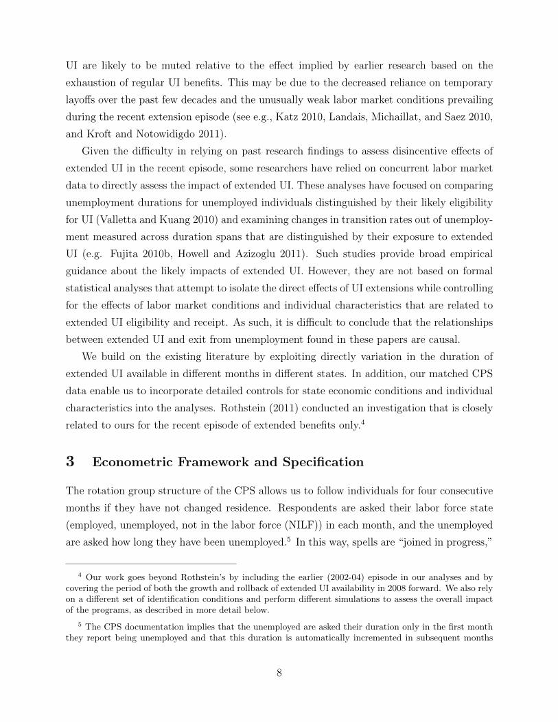
Figure 1: Variation in Total Weeks of UI Available

5

Figure 1 illustrates the variation in eligibility for extended UI over time (years 2000-2012)

based on the various programs in effect. Panel A displays the maximum and minimum

number of total UI weeks available across states, and Panel B displays the average and

standard deviation of the distribution of total weeks of UI available across unemployed

individuals (measured using a sample of all individuals identified as unemployed and eligible

to receive UI in the CPS microdata; see our definition of eligibility below). The spread

between the maximum and minimum number of weeks was similar between the most recent

episode and the preceding episode in the early 2000s, at about 26-27 weeks. However, the

number of states at or near the minimum in the recent episode, and their size, was much

smaller than in the preceding episode. This is reflected in Panel B, which shows that the

average weeks of total UI eligibility reached about 96 in late 2009, implying that the typical

unemployed individual was located in a state in which maximum UI eligibility was 99 weeks.

In the early 2000s, maximum weeks of eligibility reached 72, but few states triggered on to

the maximum extensions, and only about 13 additional weeks of UI beyond the normal 26

were available to the typical unemployed individual. The standard deviation displayed in

Panel B (on a separate scale, on the right side of the graph) indicates that the dispersion

in total weeks available was only slightly higher in the recent episode than in the preceding

one, implying that there is a similar degree of cross-state variation used for our estimates in

both episodes. Panel B shows a sharp drop in 2012 in the average number of weeks of UI

for which unemployed individuals qualify, as implied by the discusion of the legislation in

Appendix I.

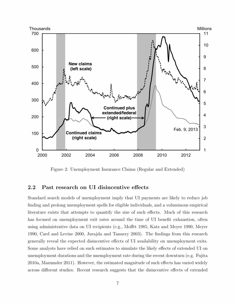
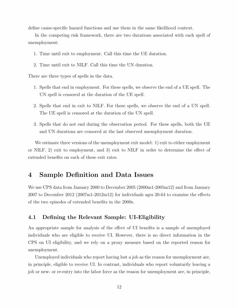
Figure 2 illustrates the expansion of UI receipt during the recent recession and subsequent

reduction as the labor market recovery has proceeded. The weekly flow of new UI claims

peaked at about 660 thousand in early 2009 (slightly below the peak of nearly 700 thousand

reached in late 1982; not shown). As of early 2013, new UI claims had declined to nearly

their pre-recession level. In addition to the weekly flow of new UI claims, two series for

the level of ongoing UI claims are displayed in figure 2: 1) regular UI claims (26 or fewer

weeks) and 2) regular UI claims plus UI claims available through extensions. The level of

both series has declined by about half since peaking in late 2009 and early 2010. The sharp,

temporary drop in mid-2010 corresponds to the suspension period of June-July 2010. A

much smaller but still substantial number of extended claimants also were present during

the earlier episode of UI extensions during 2002-2004.

6

1

2

3

4

5

6

7

8

9

10

11

0

100

200

300

400

500

600

700

2000 2002 2004 2006 2008 2010 2012

Thousands Millions

New claims (left scale)

Continued plusextended/federal

(right scale)

Continued claims (right scale)

Feb. 9, 2013

Figure 2: Unemployment Insurance Claims (Regular and Extended)

2.2 Past research on UI disincentive effects

Standard search models of unemployment imply that UI payments are likely to reduce job

finding and prolong unemployment spells for eligible individuals, and a voluminous empirical

literature exists that attempts to quantify the size of such effects. Much of this research

has focused on unemployment exit rates around the time of UI benefit exhaustion, often

using administrative data on UI recipients (e.g., Mofftt 1985, Katz and Meyer 1990, Meyer

1990, Card and Levine 2000, Jurajda and Tannery 2003). The findings from this research

generally reveal the expected disincentive effects of UI availability on unemployment exits.

Some analysts have relied on such estimates to simulate the likely effects of extended UI on

unemployment durations and the unemployment rate during the recent downturn (e.g. Fujita

2010a, Mazumder 2011). However, the estimated magnitude of such effects has varied widely

across different studies. Recent research suggests that the disincentive effects of extended

7

UI are likely to be muted relative to the effect implied by earlier research based on the

exhaustion of regular UI benefits. This may be due to the decreased reliance on temporary

layoffs over the past few decades and the unusually weak labor market conditions prevailing

during the recent extension episode (see e.g., Katz 2010, Landais, Michaillat, and Saez 2010,

and Kroft and Notowidigdo 2011).

Given the difficulty in relying on past research findings to assess disincentive effects of

extended UI in the recent episode, some researchers have relied on concurrent labor market

data to directly assess the impact of extended UI. These analyses have focused on comparing

unemployment durations for unemployed individuals distinguished by their likely eligibility

for UI (Valletta and Kuang 2010) and examining changes in transition rates out of unemploy-

ment measured across duration spans that are distinguished by their exposure to extended

UI (e.g. Fujita 2010b, Howell and Azizoglu 2011). Such studies provide broad empirical

guidance about the likely impacts of extended UI. However, they are not based on formal

statistical analyses that attempt to isolate the direct effects of UI extensions while controlling

for the effects of labor market conditions and individual characteristics that are related to

extended UI eligibility and receipt. As such, it is difficult to conclude that the relationships

between extended UI and exit from unemployment found in these papers are causal.

We build on the existing literature by exploiting directly variation in the duration of

extended UI available in different months in different states. In addition, our matched CPS

data enable us to incorporate detailed controls for state economic conditions and individual

characteristics into the analyses. Rothstein (2011) conducted an investigation that is closely

related to ours for the recent episode of extended benefits only.4

3 Econometric Framework and Specification

The rotation group structure of the CPS allows us to follow individuals for four consecutive

months if they have not changed residence. Respondents are asked their labor force state

(employed, unemployed, not in the labor force (NILF)) in each month, and the unemployed

are asked how long they have been unemployed.5 In this way, spells are “joined in progress,”

4 Our work goes beyond Rothstein’s by including the earlier (2002-04) episode in our analyses and bycovering the period of both the growth and rollback of extended UI availability in 2008 forward. We also relyon a different set of identification conditions and perform different simulations to assess the overall impactof the programs, as described in more detail below.

5 The CPS documentation implies that the unemployed are asked their duration only in the first monththey report being unemployed and that this duration is automatically incremented in subsequent months

8

leading to the classic problem of length-biased sampling. This produces a sample of longer

spells than the overall distribution of unemployment spells, and our econometric model needs

to account for this.6

We use a simple discrete-time hazard specification to model the probability that an

unemployment spell ends at duration S given that it has lasted at least until S. This hazard

function is h(S), where h(·) is a probability function (e.g., probit or logit) that will also

depend on a set of individual and labor market characteristics as well as the duration of

unemployment. Assuming independence across months, the unconditional probability that

a spell of unemployment ends at duration S (to either employment or NILF) is

P (D = S) = h(S)S−1∏t=1

(1− h(t)). (1)

In the case where a spell remains in progress with duration S at the last survey in which it

is observed, what is known is that the duration of the spell is at least S. The unconditional

probability that a spell of unemployment has duration at least S (the survivor function) is

G(S) = P (D ≥ S) =S∏

t=1

(1− h(t)). (2)

The short-panel structure of the CPS implies that only unemployment spells lasting

long enough to make it to the survey date are measured. Let S0 represent the duration

of an unemployment spell when it is first observed in the CPS. Now suppose there are

n observations subsequent to the first observation of the unemployment spell where the

individual remains unemployed or is first observed to have exited unemployment (either to

employment or NILF). Given that spells are not observed unless they reach duration S0, the

appropriate conditional probability of a spell ending with duration S is

P (D = S|D ≥ S0) =h(S)

∏S−1t=1 (1− h(t))∏S0−1

t=1 (1− h(t))= h(S)

S−1∏t=S0

(1− h(t)). (3)

for which they report being unemployed. In fact, the sequences of spell durations are not this clean. Inaddition, as reported by Elsby, Hobijn, Sahin, and Valletta (2011), in the matched CPS data many individualsidentified as newly unemployed in a month report durations of unemployment that substantially exceed onemonth.

6 The durations-to-date of the spells in progress in a cross-section is a misleading guide to the durationof a randomly selected set of completed spells. Later, we use our estimates of the model of exit fromunemployment to simulate the effect of extended benefits on the steady-state distribution of duration ofspells in progress in a cross-section.

9

Analogously, the appropriate conditional probability for a spell that remains in progress with

duration S when it is last observed is

P (D ≥ S|D ≥ S0) =

∏St=1(1− h(t))∏S0−1t=1 (1− h(t))

=S∏

t=S0

(1− h(t)). (4)

These conditional probabilities appropriately account for the length-biased sampling problem

and allow inference about the overall distribution of unemployment durations.

The likelihood function appropriate to this model is derived from equations 3 and 4.

Assuming a standard normal CDF for the hazard probability, the result is a probit model

where each monthly observation on an unemployment spell (matched to the succeeding

month) contributes to the likelihood function. Monthly observations where the spell has not

ended by the next month have a “zero” outcome with the probability specified in equation

4. Monthly observations where the spell has ended by the next month have a “one” outcome

with the probability specified in equation 3. Each spell in the sample has at most one

observation with a “one” outcome (the end of the spell).

A specification choice must be made regarding how to characterize the availability of

extended benefits in the model. Based on past research findings regarding exhaustion spikes

and our preliminary specification search, the approach we selected includes two indicator

variables for the availability of unemployment insurance benefits to the worker.

1. EBit – An indicator for availability of extended benefits at time t which equals one

if 1) individual i has been unemployed for fewer months than the number of months

of UI available (including extended benefits) in the relevant state and months and 2)

some extended benefits are available in the relevant state and month.7

2. Lastit – An indicator which equals one if individual i is in the last month of his/her

UI availability at time t. This is meant to allow for a spike in the exit hazard at

exhaustion.

The probit model is specified by assuming a spell ends in a given month if an unobserved

latent variable for spell i in month t (yit) is positive. This latent variable is

yit = Xitβ + δ1EBit + δ2Lastit + εit, (5)

7 Our empirical models include indicator (dummy) variables for each of the first six months of unemploy-ment. The EB availability indicator therefore captures the marginal effect of extended benefits. Rothstein(2011) found that the recent episode of extended benefits had significant effects on exit rates only for in-dividuals unemployed for at least 6 months, which suggests that we are not missing an important effect ofextended benefits with our specification choice.

10

where Xit is a vector of individual and economic variables, β is a vector of parameters,

δ1 is a parameter measuring the marginal effect of extended benefits on the hazard of an

unemployment spell ending, δ2 is a parameter measuring the marginal effect on the hazard

of being in the last month of UI eligibility, and εit is an error term with a standard normal

distribution. The hazard of a spell ending is then

h(t) = P (Yit > 0) = P (−εit < Xitβ+ δ1EBit + δ2Lastit) = Φ(Xitβ+ δ1EBit + δ2Lastit), (6)

where Φ(·) is the standard normal cumulative distribution function.

The estimated model includes in the X vector a set of standard personal characteristics

that are systematically related to labor market outcomes: 4 education categories, 5 age cate-

gories (covering the included ages 20-64), and indicators for female, married, female*married,

and nonwhite individuals. In order to account for local labor market conditions, the model

includes a cubic in the monthly seasonally adjusted state unemployment rate and a cubic

in the 3-month annualized growth in seasonally adjusted log non-farm payroll employment.

To allow for a flexible baseline hazard and to account for the effects of normal UI benefits,

the model also includes a set of indicators for the first 6 months of unemployment (0-6) and

single indicators for months 7-9, months 10-12, and months 13-28 (9 categories in total).

We also include a complete set of date (year-month) and state indicators, which provide

additional controls for relative economic conditions that are shared across all states but vary

over time and relative conditions that are state-specific and fixed over time.

To summarize, our hazard model of the exit from unemployment includes fixed effects

for each state and each month, along with individual duration, demographic characteristics,

and measures of local economic conditions. As such, identification of the effect of extended

benefits in this model comes from within-state variation over time and cross-state variation

at a point in time in the availability of extended benefits, conditional on the other factors in

the model.

3.1 A Competing Risk Model

We apply the probit model developed here to the probability that an individual exits un-

employment, regardless of the subsequent labor force state. It is also interesting to explore

how extended benefits affect both the probability of exiting unemployment to a job (employ-

ment) and probability of exiting unemployment to leave the labor force (cease searching). A

competing risk framework is natural for this purpose and can be implemented as a straight-

forward generalization of the discrete choice hazard model outlined above. The key is to

11

define cause-specific hazard functions and use them in the same likelihood context.

In the competing risk framework, there are two durations associated with each spell of

unemployment:

1. Time until exit to employment. Call this time the UE duration.

2. Time until exit to NILF. Call this time the UN duration.

There are three types of spells in the data.

1. Spells that end in employment. For these spells, we observe the end of a UE spell. The

UN spell is censored at the duration of the UE spell.

2. Spells that end in exit to NILF. For these spells, we observe the end of a UN spell.

The UE spell is censored at the duration of the UN spell.

3. Spells that do not end during the observation period. For these spells, both the UE

and UN durations are censored at the last observed unemployment duration.

We estimate three versions of the unemployment exit model: 1) exit to either employment

or NILF, 2) exit to employment, and 3) exit to NILF in order to determine the effect of

extended benefits on each of these exit rates.

4 Sample Definition and Data Issues

We use CPS data from January 2000 to December 2005 (2000m1-2005m12) and from January

2007 to December 2012 (2007m1-2012m12) for individuals ages 20-64 to examine the effects

of the two episodes of extended benefits in the 2000s.

4.1 Defining the Relevant Sample: UI-Eligibility

An appropriate sample for analysis of the effect of UI benefits is a sample of unemployed

individuals who are eligible to receive UI. However, there is no direct information in the

CPS on UI eligibility, and we rely on a proxy measure based on the reported reason for

unemployment.

Unemployed individuals who report having lost a job as the reason for unemployment are,

in principle, eligible to receive UI. In contrast, individuals who report voluntarily leaving a

job or new- or re-entry into the labor force as the reason for unemployment are, in principle,

12

not eligible to receive UI. While losing a job is a necessary condition for being eligible to

receive UI benefits, it is not sufficient. For example, a worker who reports a job loss may

not have sufficient previous employment experience to qualify for unemployment insurance

or may have been fired for cause.8

Because we do not have the detailed work-history information needed to impute eligibility,

we proceed by classifying unemployed job losers as the UI-eligible group that we use in our

analysis. Job leavers and new labor force entrants are classified as UI-ineligible and are not

included in our analysis. Later, we present a “placebo” analysis of the effect of extended

benefits on exit from unemployment for the UI-ineligible sample (job leavers and new entrants

to the labor force). We expect the effects of extended UI for this group to be smaller than

for UI eligible individuals. However, if there is variation in economic conditions across

states over time that is correlated with the availability of extended benefits but that is not

accounted for by the variables in the model, we could find that exits from unemployment for

the ineligible group is related to extended UI simply due to this omitted variable problem.

Such a finding would imply that our estimates of the effect of extended UI on the UI-eligible

group may be too large and would represent an upper bound on the true effect. Working

in the opposite direction, there may be spillover effects on job search and job finding from

eligible to ineligible individuals that would show up as a positive relationship between exit

from unemployment and extended UI for the UI-ineligible group (Levine, 1993).9

Table 1 provides supporting evidence for our working definition of UI eligibility. Each

March, the regular monthly CPS is accompanied by an extensive set of supplemental ques-

tions regarding income receipt in the prior calendar year; UI is separately identified as an

individual income source. The rotating sample structure of the CPS enables matching of

observations on unemployed individuals for selected months in year t with the information

on their income receipt in year t recorded in the year t + 1 March supplement. Based on

this match, table 1 provides a breakdown of UI income receipt (percent reporting positive

UI income) by measured eligibility status for individuals who are unemployed in March or

December of the calendar year corresponding to reported income receipt, for income years

8 Another consideration is that an eligible worker may choose not to take up benefits. However, thedecision to take up benefits may be affected by the structure of the UI program, including the availability ofextended benefits, so that is would not be appropriate to restrict the analysis only to those eligible workerswho choose to take up benefits. And since we have no data in the monthly CPS that would allow us todetermine actual UI receipt, we cannot make this sample distinction in any case.

9 Levine’s empirical results suggest that the UI-induced reduction in job finding within the group ofUI-eligibles increases job availability and hence the job-finding rate for ineligibles.

13

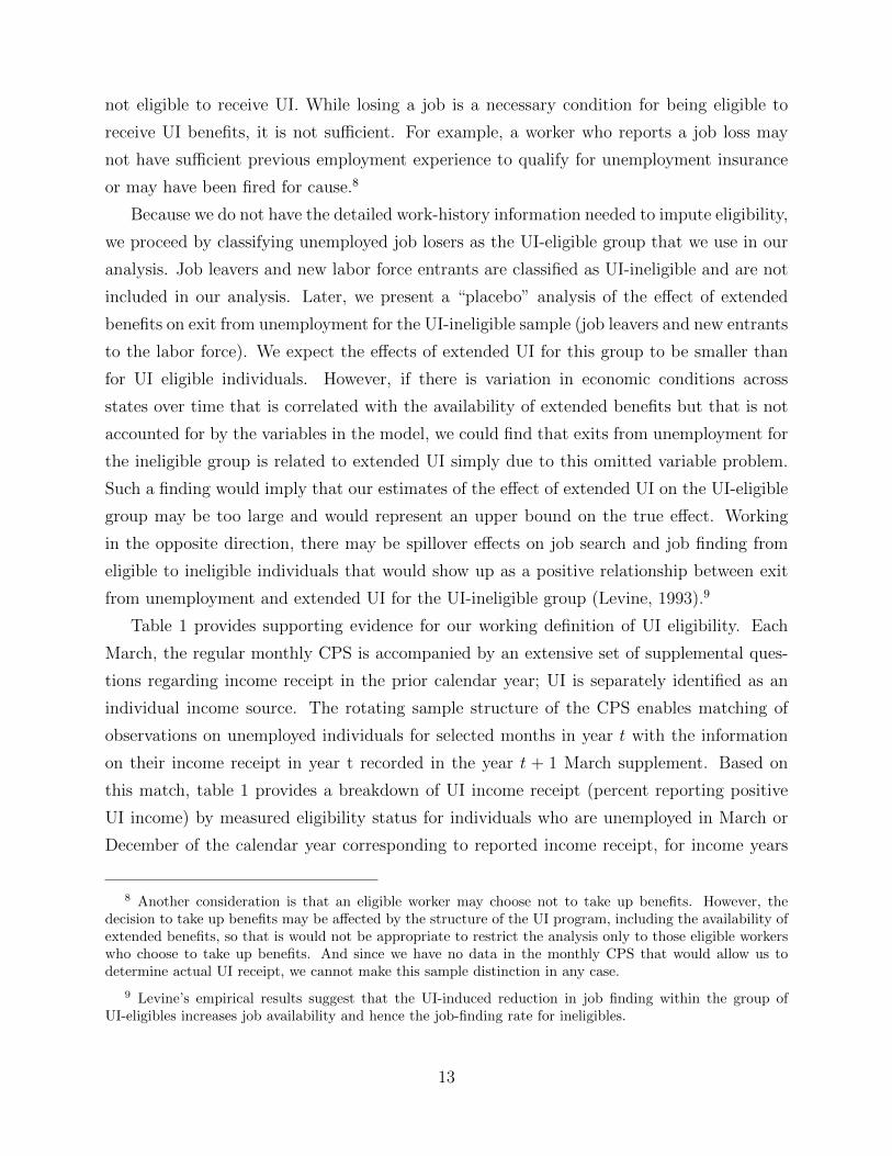
Table 1: UI Income Receipt, by Eligibility Status

(unemployed in base month, matched to subsequent March survey)

2005-2011. The percentage of the UI-eligible who report receiving UI income reached about

50 percent in 2009 and has declined somewhat since then. The percentage of the UI-ineligible

who report receiving UI income is much lower, usually at about 5-10 percent, with a few

higher values recorded. Because individuals may be subject to multiple unemployment spells

over a calendar year, an unknown proportion of individuals identified as ineligible in a par-

ticular month may have received UI income based on a separate spell of unemployment that

year, for which they were eligible for UI receipt based on their stated reason for unemploy-

ment. On balance, we interpret these figures as suggesting that our eligibility indicator is

strongly correlated with actual eligibility status, although take-up of unemployment insur-

ance by those eligible is clearly not universal.10

4.2 Sample Construction: Matching the Monthly CPS

The rotation group structure of the CPS visits a given address (housing unit) for four months,

does not interview for eight months, and revisits the address for four more months. In other

words, over a 16 month period, the household is surveyed for four months, left alone for

eight months, and surveyed for four more months. This sample structure allows us to match

10 See Blank and Card (1991) and Anderson and Meyer (1997) for earlier studies of incomplete take-uprates for unemployment insurance.

14

households in consecutive months up to three times. Failures to match primarily occur when

a household moves to a new housing unit between interviews. This generally occurs less than

five percent of the time.

One key concern with regard to use of the matched data is the likelihood of spurious tran-

sitions in labor force status, particularly spurious exits from unemployment, that can lead to

an overestimate of the probability of exit from unemployment (e.g., Abowd and Zellner, 1985;

Poterba and Summers, 1986, 1995). As demonstrated by Rothstein (2011), the unemploy-

ment durations implied by the frequency and duration structure of exits from unemployment

are much lower than the reported durations of spells in progress in the cross-section.11 This

difference in distributions is due in part to the length-biased sampling inherent in an analysis

of durations of spells in progress in a cross-section. But the difference is also the result of the

likely presence of spurious transitions. These spurious transitions are potentially problematic

for the estimation of our models, since errors in the identification of exit from unemployment

could seriously bias the estimates of the effects of extended benefits.

Following Rothstein (2011), we address this problem through direct adjustments to re-

ported transitions following specific patterns that are indicative of reporting errors. In par-

ticular, for individuals who report a transition out of unemployment in month one followed

immediately by an entry back to unemployment in month three, we recode the intervening

month as a continuation of the initial unemployment spell. We do this whether the unem-

ployment exit is due to job finding or labor force withdrawal. In other words, letting U

represent unemployment, E employment, and N out of the labor force, we recode 3-month

transition patterns of UEU and UNU to UUU, and we retain both of the resulting UU ”tran-

sitions” in the matched data. We recoded 3,016 UEU transitions and 7,119 UNU transitions

(a total of 10,135 transitions) in our estimation samples in this way.12

Some support for the idea that UEU and UNU transitions are likely to be spurious is that

reported unemployment durations in the third month of observed UEU and UNU transitions

is, on average, far greater than one month (average of 5.7 months, median of 3 months). As

noted by Elsby et al. (2011), it is likely that individuals’ reported unemployment duration

reflects the time elapsed since the loss of a salient job, which is likely the one that enabled

11 We confirmed that this is not due to the construction of the matched CPS sample. The distributionof reported durations from the sample, treated as a series of cross-sections, is essentially identical to thedistribution from the complete CPS cross sections.

12 Of these 10,135 recoded transitions, 5,008 were for UI-eligible spells and 5,127 were for UI-ineligiblespells.

15

.1.2

.3.4

.5.6

0 2 4 6 8 10 12 14 16 18 20 22 24Months Unemployed

Observed Exit Rate Adjusted Exit Rate (UEU,UNU->UUU)

Exit

Rate

Source: Authors' calculations from matched CPS 2000-2012m10.

Figure 3: Exit Rate from Unemployment, Observed and Adjusted (UEU,UNU − > UUU)

them to qualify for UI benefits. The reported durations are therefore much more likely to

capture the duration of a spell of ongoing UI receipt than are the durations implied by

reported unemployment exits, which may reflect stopgap jobs and temporary labor force

withdrawals in additional to direct reporting errors (see also Poterba and Summers, 1995).

Figure 3 contains a plot of average (over the 2000-2012 period) exit rates from unem-

ployment by duration of unemployment. Two exit rates are presented: 1) the observed exit

rate and 2) the exit rate adjusted by recoding UNU and UEU sequences to UUU (no exit).

Clearly, the adjustment substantially reduces the exit rates from unemployment, implying

an increase in the survivor function and associated unemployment durations.13

Imposing this adjustment to observed transitions requires restricting the set of observa-

tions we use to those from the first two of each set of four consecutive CPS rotation groups,

so that we have at least two subsequent matched observations. We impose this restriction

and the transition adjustment for all of our analysis samples. As such, although we have

CPS data through December 2012, our final observation is for October 2012. In addition,

to ensure valid matches of individuals across months, we dropped a small number of obser-

vations for which reported age, gender, race, and educational attainment are not consistent

across months (i.e., age changes by more than 1 year, etc.).

13 Rothstein (2011) presents a graph (Figure 7, page 182) of the Kaplan-Meier survivor functions withand without recoding of the UEU and UNU transitions to UUU.

16

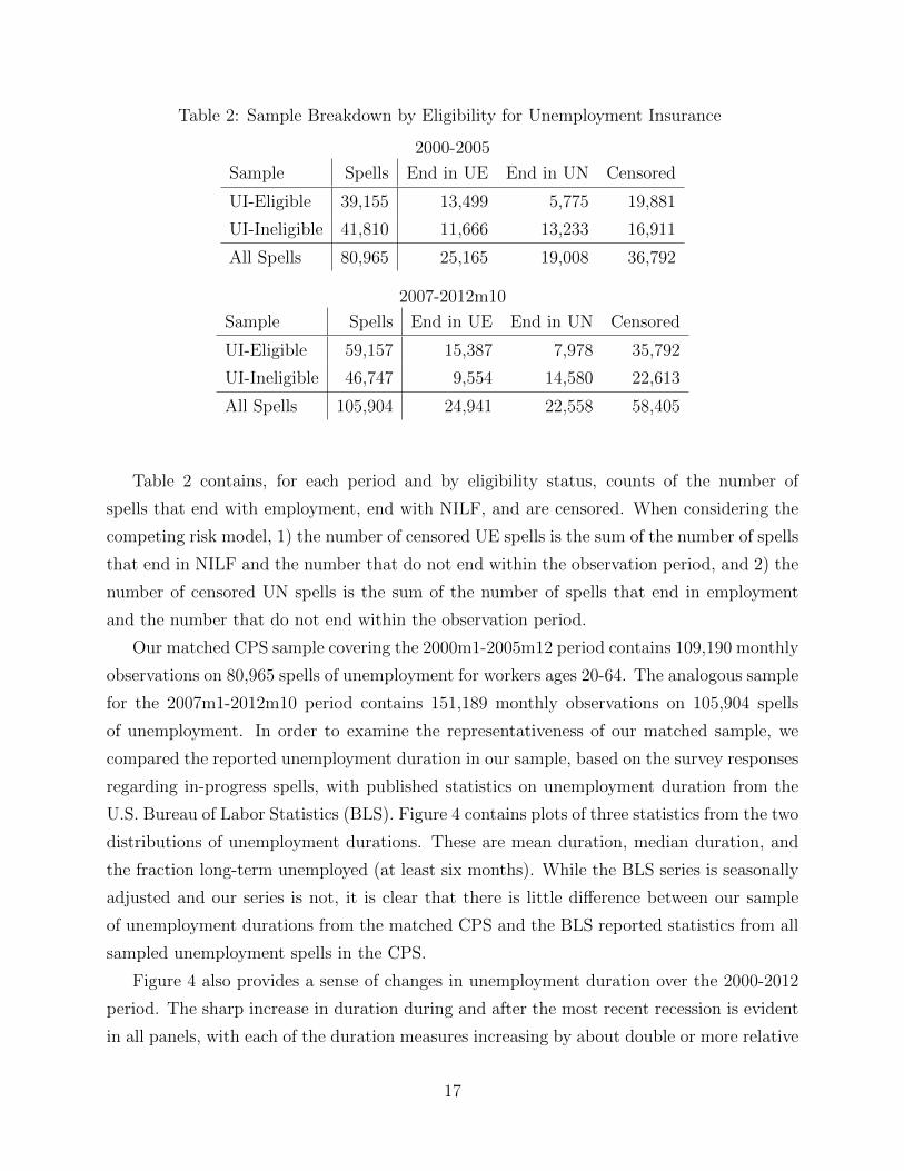
Table 2: Sample Breakdown by Eligibility for Unemployment Insurance

2000-2005

Sample Spells End in UE End in UN Censored

UI-Eligible 39,155 13,499 5,775 19,881

UI-Ineligible 41,810 11,666 13,233 16,911

All Spells 80,965 25,165 19,008 36,792

2007-2012m10

Sample Spells End in UE End in UN Censored

UI-Eligible 59,157 15,387 7,978 35,792

UI-Ineligible 46,747 9,554 14,580 22,613

All Spells 105,904 24,941 22,558 58,405

Table 2 contains, for each period and by eligibility status, counts of the number of

spells that end with employment, end with NILF, and are censored. When considering the

competing risk model, 1) the number of censored UE spells is the sum of the number of spells

that end in NILF and the number that do not end within the observation period, and 2) the

number of censored UN spells is the sum of the number of spells that end in employment

and the number that do not end within the observation period.

Our matched CPS sample covering the 2000m1-2005m12 period contains 109,190 monthly

observations on 80,965 spells of unemployment for workers ages 20-64. The analogous sample

for the 2007m1-2012m10 period contains 151,189 monthly observations on 105,904 spells

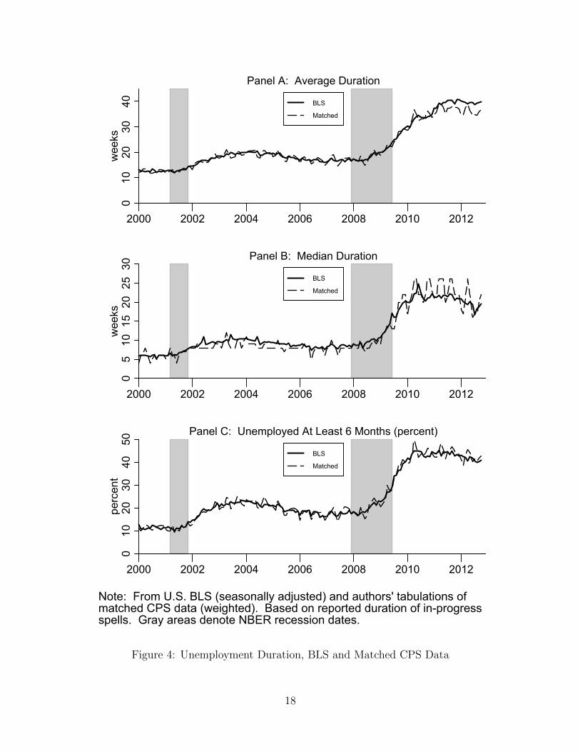
of unemployment. In order to examine the representativeness of our matched sample, we

compared the reported unemployment duration in our sample, based on the survey responses

regarding in-progress spells, with published statistics on unemployment duration from the

U.S. Bureau of Labor Statistics (BLS). Figure 4 contains plots of three statistics from the two

distributions of unemployment durations. These are mean duration, median duration, and

the fraction long-term unemployed (at least six months). While the BLS series is seasonally

adjusted and our series is not, it is clear that there is little difference between our sample

of unemployment durations from the matched CPS and the BLS reported statistics from all

sampled unemployment spells in the CPS.

Figure 4 also provides a sense of changes in unemployment duration over the 2000-2012

period. The sharp increase in duration during and after the most recent recession is evident

in all panels, with each of the duration measures increasing by about double or more relative

17

010

2030

40w

eeks

2000 2002 2004 2006 2008 2010 2012

BLS

Matched

Panel A: Average Duration

05

1015

2025

30w

eeks

2000 2002 2004 2006 2008 2010 2012

BLS

Matched

Panel B: Median Duration

010

2030

4050

perc

ent

2000 2002 2004 2006 2008 2010 2012

BLS

Matched

Panel C: Unemployed At Least 6 Months (percent)

Note: From U.S. BLS (seasonally adjusted) and authors' tabulations ofmatched CPS data (weighted). Based on reported duration of in-progressspells. Gray areas denote NBER recession dates.

Figure 4: Unemployment Duration, BLS and Matched CPS Data

18

Table 3: Unemployment Survivor Rates, by Duration in Months (UI Eligible Sample)

Months (1) (2) (3) (4)

Duration 2000-2005 2002m3-2004m2 2007-2012m10 2009-2011

1 0.474 0.499 0.501 0.523

2 0.296 0.328 0.337 0.366

3 0.202 0.233 0.246 0.276

4 0.143 0.166 0.185 0.215

5 0.105 0.127 0.143 0.168

6 0.077 0.099 0.113 0.137

7 0.053 0.074 0.088 0.111

8 0.041 0.059 0.072 0.092

9 0.030 0.044 0.059 0.076

10 0.023 0.035 0.048 0.062

11 0.018 0.027 0.040 0.053

12 0.013 0.021 0.033 0.044Note: Authors’ calculations from matched CPS data (weighted).

to their pre-recession values.

The unemployment durations in figure 4 come from the cross-sectional distribution of

spells in progress. As noted earlier, due to the length-biased sampling problem, this distri-

bution is likely to overstate the duration distribution for all spells of unemployment. This

is implied by the tabulations of survivor rates of unemployment spells in table 3, for which

we used our matched data to calculate survivor rates across months during the first year

of unemployment. This table displays the tabulations separately for our two estimation

samples (2000-2005 in column 1 and 2007-2012m10 in column 3). In order to highlight the

higher unemployment survivor rates in the weakest labor market periods, the table also dis-

plays survivor rates for sub-periods with availability of extended benefits and relatively high

unemployment rates (2002m3-2004m2 in column 2 for the earlier period and 2009-2011 in

column 4 for the later period). The exit rates from unemployment are sufficiently high that

only a small fraction of individuals remain unemployed after the first six months. In the

weak labor market from 2002-2004, only about 10 percent of unemployment spells for job

losers (our UI-eligible sample) lasted past 6 months. In the very weak labor market from

2009-2011, 13.7 percent of job losers remained unemployed for at least 6 months.

On inspection, it appears that the survivor rates presented in table 3 are not consistent

with the cross-section distribution of durations of incomplete spells calculated directly from

the CPS. For example, in the 2009-2011 period, the survival rate at 6 months 13.7 percent

19

while 39.8 percent of spells in progress in the cross-section in this period were at least 6

months. This is largely a result of the length biased sampling built into the cross-section

that results in over-sampling of long spells. Later we present estimates of the cross-section

distribution of spells in progress implied by our model of exits that reconciles much of this

difference. Our analysis highlights the inappropriateness of making inferences about the

distribution of completed spells from the cross-section distribution of spells in progress.

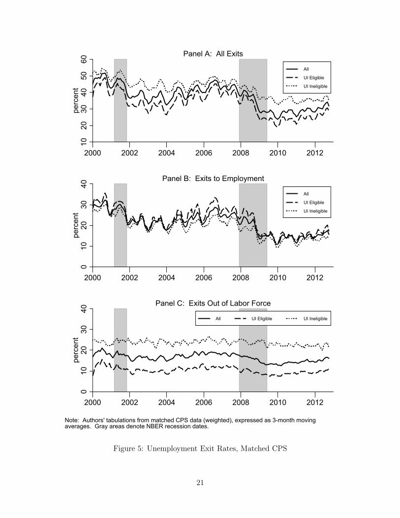
Figure 5 complements table 3 by showing monthly exit rates from unemployment over

our complete sample tabulated for all exits in Panel A and exits by type (to employment

or out of the labor force) in Panels B and C. In each case, we display the exit rates for

all unemployed individuals and also for UI eligible and ineligible individuals separately. A

sharp decline in exit rates, particularly exits to employment, is evident during the recent

recession, with a minor rebound evident beginning in 2010. Overall exit rates are higher for

UI-ineligible individuals than for eligible individuals, which reflects the large gap between

the two groups for exits out of the labor force (Panel C). The rates of labor force exit from

unemployment exhibit very little cyclicality, with only a slight net decline evident during

the recent recession and essentially no cyclicality evident for UI ineligibles.

5 Estimation of the Probit Model of Exit

We present estimates of the probit model, specified in equations 5 and 6, of the probabil-

ity that an unemployment spell ends in a given month. The key parameters we estimate

representing the effect of extended benefits on the unemployment exit probability are δ1

(the coefficient on the EB indicator) and δ2 (the coefficient on the Last indicator for the

final month of UI eligibility). As specified in equation 5, the underlying estimated probit

parameter on EB is δ1, and the average marginal effect of EB on the probability of exit

from unemployment is computed from this as

δ∗1 = δ11

N

∑i,t

φ(Xitβ + δ1EBit + δ2Lastit), (7)

where φ(·) is the standard normal probability density function and N is the sample size.

Analogously, the average marginal effect of exhaustion of UI (indicated by Last) on the

probability of exit is

δ∗2 = δ21

N

∑i,t

φ(Xitβ + δ1EBit + δ2Lastit). (8)

20

1020

3040

5060

perc

ent

2000 2002 2004 2006 2008 2010 2012

All

UI Eligible

UI Ineligible

Panel A: All Exits

010

2030

40pe

rcen

t

2000 2002 2004 2006 2008 2010 2012

All

UI Eligible

UI Ineligible

Panel B: Exits to Employment

010

2030

40pe

rcen

t

2000 2002 2004 2006 2008 2010 2012

All UI Eligible UI Ineligible

Panel C: Exits Out of Labor Force

Note: Authors' tabulations from matched CPS data (weighted), expressed as 3-month movingaverages. Gray areas denote NBER recession dates.

Figure 5: Unemployment Exit Rates, Matched CPS

21

Table 4: Estimated Average Marginal Effects on Probability of Exit from Unemployment

UI Eligible Sample

2000-2005m2 2007-2012m10

Model δ∗1 δ∗2 δ∗1 δ∗2Single Risk -0.0583 0.0538 -0.0500 0.0220

(0.0138) (0.0156) (0.0064) (0.0199)

Exit to Emp -0.0212 0.0263 -0.0099 0.0208

(0.0121) (0.0150) (0.0065) (0.0129)

Exit to NILF -0.0372 0.0287 -0.0340 0.0040

(0.0106) (0.0098) (0.0033) (0.0109)

Note: δ∗1 is the average marginal effect on the exit probability of the indicator for availability

of extended benefits. δ∗2 is the average marginal effect of the indicator for the last month of

availability of benefits. These are calculated using equations 7 and 8. The probit model also

includes controls for 4 education categories, 5 age categories (covering the included ages 20-64),

female, married, female*married, nonwhite, year-month indicators, state indicators, a cubic in the

monthly seasonally adjusted state unemployment rate, a cubic in the 3-month annualized growth

in seasonally adjusted log non-farm payroll employment, a set of indicators for the first 6 months

of unemployment (0-6) and single indicators for months 7-9, months 10-12, and months 13-28 (9

categories for duration in total). The estimates are weighted by the CPS sampling weights, and

robust asymptotic standard errors clustered by state are in parentheses. The sample for 2000-

2005m12 includes 44,367 matched monthly observations on 31,925 spells of unemployment for job

losers. The sample for 2007-2012m10 includes 81,472 matched monthly observations on 54,928

spells of unemployment.

Note that both of these marginal effects could be important in measuring the effect of

extended benefits because extended benefits increase the number of periods for which an

individual can receive UI and any spike in the exit probability at exhaustion is pushed

further into the unemployment spell when extended benefits are available.

Estimates of the key parameters from six versions of the probit model of exit from unem-

ployment are presented in table 4. There are three models for each of the two time periods

(2000-2005 and 2007-2012m3) with a period of extended benefits. Within each time period,

there is a model of exit from unemployment and two models representing the competing risks

of exit to employment and exit to NILF. There is a clear pattern to the estimates. In both

time periods and in the single risk and in the competing risk model for exit from the labor

force, the availability of extended benefits has a substantial negative effect on the probability

of exit from unemployment (indicated by δ∗1). These effects are comparable across the two

time periods. There is no significant effect of extended benefits on the probability of exit

22

to employment (the job-finding rate). This suggests that the negative effect of extended

benefits on the exit rate from unemployment is driven largely by individuals staying in the

labor force longer, perhaps to collect benefits, rather than by individuals reducing search

effort and taking longer to find jobs. This pattern is consistent across the two time periods.

The evidence in table 4 on the effect of exhaustion of benefits on exit from unemployment

is mixed. This is represented by δ∗2, the average marginal effect of being in the last month

of UI eligibility on the probability of exit. In the earlier time period, the exit rate from

unemployment and the exit to NILF are significantly higher in the last month of eligibility

for UI. This is another mechanism through which extended benefits can increase the duration

of unemployment spells. The availability of extended benefits pushes the exhaustion spike

deeper into the spell of unemployment. There is no significant effect of exhaustion of benefits

on exit to employment (the job-finding rate) in the earlier period. The exhaustion of benefits

does not have a statistically significant effect on any of the exit measures in the later period.

5.1 A Placebo Test: UI-Ineligible Spells

We defined the UI eligible group to be those who report a job loss as their reason for

unemployment. The remaining unemployed report being a job leaver (quit) or a labor force

entrant (new entry or re-entry) as their reason for unemployment, and we classify these

individuals as UI ineligible. While this classification scheme is not perfect, we presented

evidence in table 1 based on the March CPS that only a small fraction of job leavers and

new entrants report having received UI. This group should be largely unaffected by the

availability of extended benefits. On this basis, we re-estimate our probit model of exit

from unemployment on samples of UI ineligible unemployed individuals in order to provide

a placebo test of our estimation strategy. If we find effects of extended benefits on exit from

unemployment for the ineligible that are similar to those we present in table 4, it could

be that we have not adequately controlled for state/month specific economic conditions and

that our estimates of the effect of extended benefits are too large. A potential factor working

in the opposite direction is that there may be a positive effect of extended benefits on exit

from unemployment among the UI-ineligible resulting from spillovers from the eligible to

the ineligible. As we noted earlier, the reasoning is that, if extended benefits reduce the

job finding rate among the UI-eligible, there may be improved job opportunities for the

UI-ineligible that increase their exit rate from unemployment (Levine, 1993).

Table 5 contains the estimates of the key UI parameters (δ∗1 and δ∗2) estimated for the

sample of UI ineligible spells. In the earlier period, we estimate there to be no effect of either

23

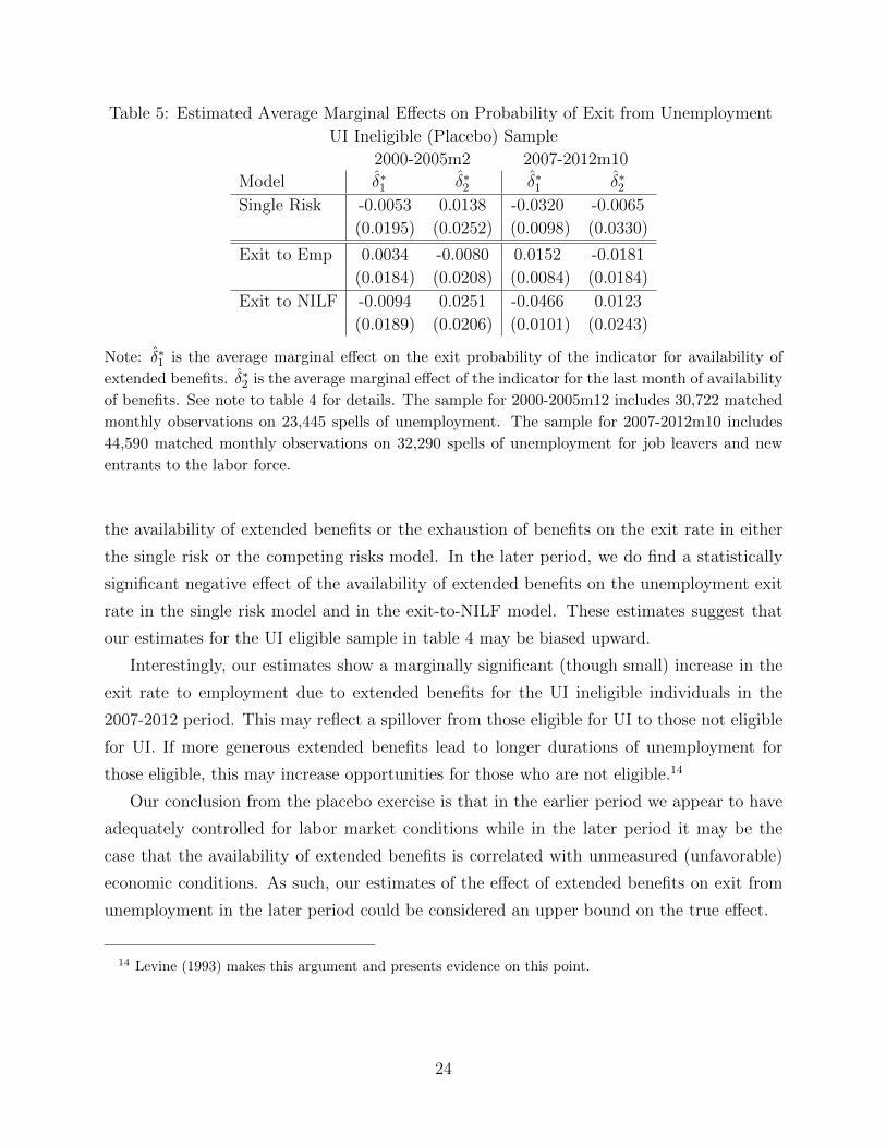
Table 5: Estimated Average Marginal Effects on Probability of Exit from Unemployment

UI Ineligible (Placebo) Sample

2000-2005m2 2007-2012m10

Model δ∗1 δ∗2 δ∗1 δ∗2Single Risk -0.0053 0.0138 -0.0320 -0.0065

(0.0195) (0.0252) (0.0098) (0.0330)

Exit to Emp 0.0034 -0.0080 0.0152 -0.0181

(0.0184) (0.0208) (0.0084) (0.0184)

Exit to NILF -0.0094 0.0251 -0.0466 0.0123

(0.0189) (0.0206) (0.0101) (0.0243)

Note: δ∗1 is the average marginal effect on the exit probability of the indicator for availability of

extended benefits. δ∗2 is the average marginal effect of the indicator for the last month of availability

of benefits. See note to table 4 for details. The sample for 2000-2005m12 includes 30,722 matched

monthly observations on 23,445 spells of unemployment. The sample for 2007-2012m10 includes

44,590 matched monthly observations on 32,290 spells of unemployment for job leavers and new

entrants to the labor force.

the availability of extended benefits or the exhaustion of benefits on the exit rate in either

the single risk or the competing risks model. In the later period, we do find a statistically

significant negative effect of the availability of extended benefits on the unemployment exit

rate in the single risk model and in the exit-to-NILF model. These estimates suggest that

our estimates for the UI eligible sample in table 4 may be biased upward.

Interestingly, our estimates show a marginally significant (though small) increase in the

exit rate to employment due to extended benefits for the UI ineligible individuals in the

2007-2012 period. This may reflect a spillover from those eligible for UI to those not eligible

for UI. If more generous extended benefits lead to longer durations of unemployment for

those eligible, this may increase opportunities for those who are not eligible.14

Our conclusion from the placebo exercise is that in the earlier period we appear to have

adequately controlled for labor market conditions while in the later period it may be the

case that the availability of extended benefits is correlated with unmeasured (unfavorable)

economic conditions. As such, our estimates of the effect of extended benefits on exit from

unemployment in the later period could be considered an upper bound on the true effect.

14 Levine (1993) makes this argument and presents evidence on this point.

24

6 How Large is the Effect of Extended Benefits?

In order to quantify the effect of extended benefits on unemployment duration, we use our

estimates to calculate the distribution of duration of unemployment spells under a set of

three alternative scenarios regarding the availability of extended benefits. We select these

alternative scenarios to facilitate comparison across the two episodes of extended benefits we

study of 1) the effects of the observed extended benefit programs and 2) the potential effects

of comparably-sized extended benefit programs. The three scenarios are

1. Observed-EB: An baseline scenario that uses the actual availability of extended benefits

in each state in a given month. This is meant to provide a reference prediction of the

survivor function and the expected duration.

2. No-EB: A scenario that assumes no extended benefits were available in any state in any

month, regardless of local labor market conditions. In comparison with the baseline,

this provides a measure of the extent to which the actual program of extended benefits

affected the distribution of duration of unemployment spells.

3. Full-EB: A scenario that assumes that 99 weeks of extended benefits were available

in all states and months during the hypothetical spells. In comparison with the no-

extended-benefits scenario, this provides a measure of the extent to which a universal

unemployment insurance program offering 99 weeks of benefits would affect the dis-

tribution of duration of unemployment spells. Without this comparison, it would be

difficult to compare the 2002-2004 with the 2008 and later experiences with extended

benefits because extended benefits in the earlier period were much less widespread.

For each scenario we estimate the expected duration of unemployment spells (E(D)) and

various quantiles of the distribution of unemployment durations (the complement of the

survivor function). We also use our estimates to calculate estimates of the distribution of

unemployment durations that would be observed in a cross-section in a steady state and how

this steady state distribution is affected by the availability of extended benefits.

We begin by creating a set of individuals starting unemployment spells based on the

characteristics of unemployed workers over the 2000m1-2012m10 period. We create a spell

for each unemployed job loser (the “eligible” group) aged 20-64. This set of 96,575 spells

reflects the wide distribution of observable characteristics among the unemployed including

demographics, human capital, and state of residence. We use this set of individuals to create

25

two hypothetical sets of unemployment spells that cover the two periods of extended benefits

in our sample:

1. March 2002 – June 2004. This period covers the early period of extended UI benefits

(running from March 2002 through Febuary 2004).15

2. January 2009 – April 2011. This period covers the end of the Great Recession and the

immediate post-recession period. Extended benefits were generally available at a very

high level throughout this period. We consider this period because the labor market

generally lags the NBER business cycle dates. For example, the peak unemployment

rate since 2007 was in 2009q4, while the NBER dated the end of the Great Recession

as 2009q2.16

For each of the three scenarios regarding extended benefits described above and based

on the estimates from the relevant probit model of unemployment exit, we predict for each

spell the monthly hazard of exit from unemployment for each month for the first 28 months

of the spell.17 We use these predicted hazards to estimate the expected duration and the

survivor function of each spell, and we present the average across spells of these quantities.

The estimated survivor function of spell i at duration t is

Gi(t) =t∏

s=1

(1− hi(s)), (9)

where hi(s) is the estimated unemployment exit probability for individual i in month s. In

order to compute the expected spell duration, we need to assume something specific about

the distribution of long spells. We assume that the monthly hazard of a spell ending after

month 28 is constant for each individual at the average value for that individual of the

15 There were also extended benefits available in Alaska in March and April 2005 due to a weak seasonallabor market and in Louisiana October 2005 through January 2006 due to Hurricane Katrina. These areincluded in the estimation of the model for the earlier period (2000-2005), but no effort is made to quantifythe effects of these small episodes.

16 We also investigated hypothetical spells for two other time periods related to the great recession. Oneran from July 2008 – October 2010. Given the fact that the labor market lags recession timing, this turnsout to be a bit early to see the very low unemployment exit rates characteristic of the weak labor marketsubsequent to the Great Recession. Another ran from July 2010 – October 2012. Given that the maximumextended benefits only began to phase out late in this period, the effects of extended benefits on the durationdistribution are virtually identical to those for the January 2009 – April 2011 period.

17 We use the exit model estimated over the 2000-2005m12 period for the March 2002 – June 2004hypothetical spells. We use the model estimated over the 2007-2012m10 period for the later spells. See table4.

26

hazard from months 24-28. The constant hazard feature of the conditional distribution of

spells longer than 28 months implies that the conditional distribution is exponential and

that the expected duration of spells from this point is simply the inverse of the constant

hazard. On this basis, the expected duration of each spell is

E(Di) =

[28∑s=1

shi(s)Gi(s− 1)

]+ Gi(28)

1

hi, (10)

where hi is the average across months 24-28 of the estimated monthly hazard of the unem-

ployment spell of individual i ending.

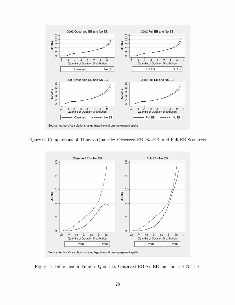
6.1 The Effect of Extended Benefits on the Duration Distribution

Figure 6 contains plots of the inverse of the CDF of unemployment duration for the sets

of hypothetical spells of unemployment corresponding to the weakest labor market in the

early 2000s (spells starting in 2002) and the weakest labor market later in the decade (spells

starting in 2009).18 In other words, these plots show the number of months required to reach

a given quantile of the duration distribution (time-to-quantile).

Each panel of figure 6 presents a comparison of the inverse CDF of durations for two

scenarios. The first row of the figure shows comparisons for the hypothetical spells beginning

in 2002 while the second row shows comparisons for hypothetical spells beginning in 2009.

The left panel in each row shows a comparison of the Observed-EB and No-EB scenarios,

while the right panel in each row shows a comparison of the Full-EB and No-EB scenarios.

In neither case is there a difference in time-to-quantile for quantiles below 0.65 or so. This

is because this quantile is reached well before 6 months and extended benefits do not have a

measurable effect on exit so early in spells. At higher quantiles for spells beginning in 2002,

the Observed-EB - No-EB difference in time-to-quantile is quite small while the Full-EB -

No-EB difference is somewhat larger. This reflects the fact, shown in figure 1, that extended

benefits were relatively less generous in the 2002-2004 period, so that the No-EB scenario

is much closer to the observed EB scenario than to the Full-EB scenario. The plots in the

second row of figure 6 for spells beginning in 2009 show an analogous pattern. At higher

quantiles, the Observed-EB - No-EB difference in time-to-quantile is similar in magnitude

to the Full-EB - No-EB difference in time-to-quantile. This reflects the fact that 99 weeks

of extended benefits were almost universally available in the 2009-2011 period, so that the

18 The inverse CDF plots months of unemployment on the vertical axis against quantiles of the durationdistribution on the horizontal axis.

27

03

69

1215

.2 .3 .4 .5 .6 .7 .8 .9 1Quantile of Duration Distribution

Observed No EB

Mon

ths

2002 Observed EB and No EB

03

69

1215

.2 .3 .4 .5 .6 .7 .8 .9 1Quantile of Duration Distribution

Full EB No EB

Mon

ths

2002 Full EB and No EB

03

69

1215

.2 .3 .4 .5 .6 .7 .8 .9 1Quantile of Duration Distribution

Observed No EB

Mon

ths

2009 Observed EB and No EB

03

69

1215

.2 .3 .4 .5 .6 .7 .8 .9 1Quantile of Duration Distribution

Full EB No EBM

onth

s

2009 Full EB and No EB

Source: Authors' calculations using hypothetical unemployment spells

Figure 6: Comparisons of Time-to-Quantile: Observed-EB, No-EB, and Full-EB Scenarios.

0.5

11.

52

2.5

.65 .7 .75 .8 .85 .9 .95 1Quantile of Duration Distribution

2002 2009

Mon

ths

Observed EB - No EB

0.5

11.

52

2.5

.65 .7 .75 .8 .85 .9 .95 1Quantile of Duration Distribution

2002 2009

Mon

ths

Full EB - No EB

Source: Authors' calculations using hypothetical unemployment spells

Figure 7: Difference in Time-to-Quantile: Observed-EB-No-EB and Full-EB-No-EB.

28

Observed-EB and Full-EB scenarios are very similar to each other and far different from the

No-EB scenario.

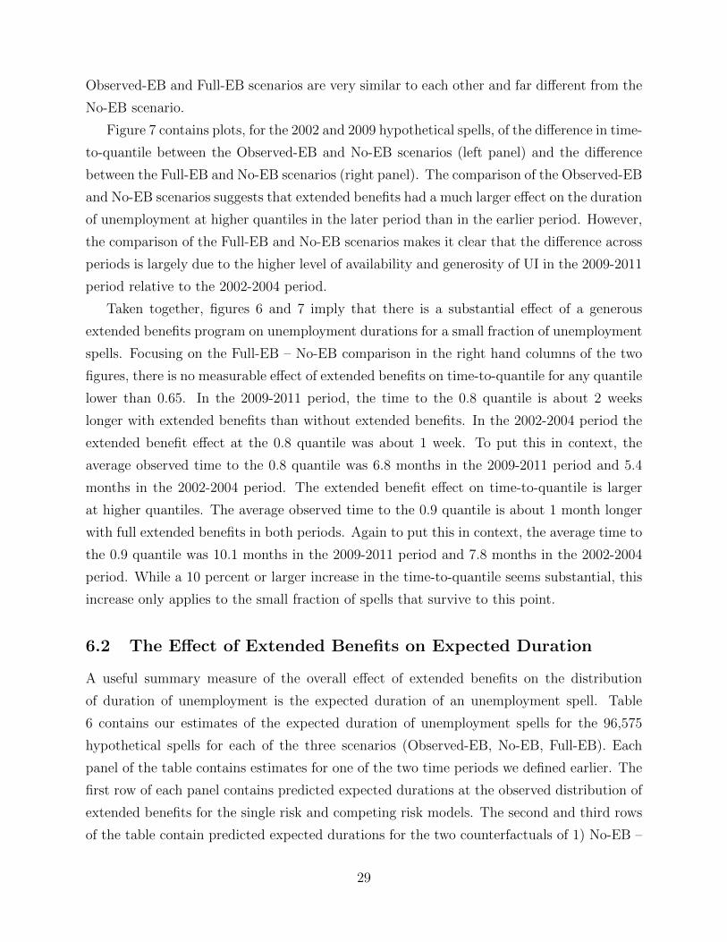
Figure 7 contains plots, for the 2002 and 2009 hypothetical spells, of the difference in time-

to-quantile between the Observed-EB and No-EB scenarios (left panel) and the difference

between the Full-EB and No-EB scenarios (right panel). The comparison of the Observed-EB

and No-EB scenarios suggests that extended benefits had a much larger effect on the duration

of unemployment at higher quantiles in the later period than in the earlier period. However,

the comparison of the Full-EB and No-EB scenarios makes it clear that the difference across

periods is largely due to the higher level of availability and generosity of UI in the 2009-2011

period relative to the 2002-2004 period.

Taken together, figures 6 and 7 imply that there is a substantial effect of a generous

extended benefits program on unemployment durations for a small fraction of unemployment

spells. Focusing on the Full-EB – No-EB comparison in the right hand columns of the two

figures, there is no measurable effect of extended benefits on time-to-quantile for any quantile

lower than 0.65. In the 2009-2011 period, the time to the 0.8 quantile is about 2 weeks

longer with extended benefits than without extended benefits. In the 2002-2004 period the

extended benefit effect at the 0.8 quantile was about 1 week. To put this in context, the

average observed time to the 0.8 quantile was 6.8 months in the 2009-2011 period and 5.4

months in the 2002-2004 period. The extended benefit effect on time-to-quantile is larger

at higher quantiles. The average observed time to the 0.9 quantile is about 1 month longer

with full extended benefits in both periods. Again to put this in context, the average time to

the 0.9 quantile was 10.1 months in the 2009-2011 period and 7.8 months in the 2002-2004

period. While a 10 percent or larger increase in the time-to-quantile seems substantial, this

increase only applies to the small fraction of spells that survive to this point.

6.2 The Effect of Extended Benefits on Expected Duration

A useful summary measure of the overall effect of extended benefits on the distribution

of duration of unemployment is the expected duration of an unemployment spell. Table

6 contains our estimates of the expected duration of unemployment spells for the 96,575

hypothetical spells for each of the three scenarios (Observed-EB, No-EB, Full-EB). Each

panel of the table contains estimates for one of the two time periods we defined earlier. The

first row of each panel contains predicted expected durations at the observed distribution of

extended benefits for the single risk and competing risk models. The second and third rows

of the table contain predicted expected durations for the two counterfactuals of 1) No-EB –

29

Table 6: Estimated Effect of Extended Benefits on Expected Duration (in Months)UI Eligible Spells

Panel 1: March 2002 – June 2004Scenario Single Risk Exit to Emp Exit to NILFObserved-EB 3.56 5.55 9.05No-EB 3.42 5.41 8.61Full-EB 3.65 5.65 9.59Observed-EB - No-EB 0.14 0.14 0.43(Obs EB - No-EB)/No-EB 0.04 0.03 0.05Full-EB - No-EB 0.23 0.24 1.02(Full-EB - No-EB)/No-EB 0.07 0.04 0.12

Panel 2: January 2009 – April 2011Scenario Single Risk Exit to Emp Exit to NILFObserved-EB 4.89 7.85 10.29No-EB 4.55 7.62 9.32Full-EB 4.89 7.85 10.24Observed-EB - No-EB 0.34 0.23 0.97(Obs EB - No-EB)/No-EB 0.07 0.03 0.10Full-EB - No-EB 0.34 0.23 0.92(Full-EB - No-EB)/No-EB 0.07 0.03 0.10

The estimates based on hypothetical samples of 96,575 spells of unemployment for each time period. Thecounterfactuals are based on the estimates of the probit model of exit from unemployment presented in table4. The expected duration is calculated from equation 10. See text for details.

no extended benefits available and 2) Full-EB – 99 weeks of extended benefits available in all

states and months. The next section of the panel shows both the absolute and proportional

differences between the average expected duration in the Observed-EB and No-EB scenarios

and the final section shows the absolute and proportional differences between the average

expected duration in the Full-EB and No-EB scenarios.

Consider first the estimates for Observed-EB in the single risk model in the first column.

The expected duration of unemployment spells beginning in March 2002 (Panel 1) averaged

3.56 months. This expected duration is intermediate between those for the No-EB and Full-

EB scenarios. Our estimates suggest that the expected duration of unemployment was 4

percent higher due to the existence of extended benefits during the 2002-2004 period. The

average expected duration of unemployment spells was substantially higher (4.89 months)

for spells beginning in January 2009 (Panel 2). Our estimates suggest that the expected

duration of unemployment was 7 percent higher due to the existence of extended benefits

during the 2009-2011 period. As we noted earlier, the larger effect of extended benefits in the

30

2009-2011 period is due to the wider availability of generous extended benefits during this

period. This is demonstrated in the last section of each panel, which show the proportional

difference in average expected duration between the Full-EB and No-EB scenario (thereby

holding constant the extent of availability). This comparison shows very similar difference

in expected durations across the two periods (7 percent in both periods).

An interesting question is what the effect of extended benefits is on the measured un-

employment rate. One very simple approach is based on two assumptions: 1) extended

benefits have no effect on the rate of entry into unemployment or into the labor force and 2)

extended benefits have no effect on exit from unemployment for job leavers or new entrants

(our UI-ineligible sample). In this case, the proportional effect of extended benefits on the

unemployment rate is equal to their proportional effect on the duration of unemployment

spells multiplied by the fraction of spells that are UI-eligible.19 On this basis, extended ben-

efits accounted for 1) 0.12 percentage points (2.2 percent) of the 5.4 percent unemployment

rate in 2003 and 2) 0.40 percentage points (4.4 percent) of the 9 percent unemployment rate

in 2010.

6.2.1 Time to Exit to Employment and NILF: The Competing Risk Model

There are at least two pathways through which extended benefits could reduce exit from

unemployment:

1. The unemployed could reduce search effort or maintain a higher reservation wage.

Either results in longer time until an unemployment spell ends in a new job.

2. The unemployed could remain attached to the labor force and searching (perhaps

minimally) when, without extended benefits, they would exit the labor force.

The competing risk model is well suited to investigating the extent to which extended benefits

works through these pathways, and the estimated effects of extended benefits on the times

until exit to employment and exit to NILF are shown in the second and third columns of

table 6 for each scenario and in each time period.

Recall that the estimated marginal effects from the probit model do not show a significant

effect of extended benefits on exit to employment (table 4). The point estimates themselves

19 We use the proportional difference between the Observed-EB expected duration and the No-EB expectedduration in table 6 as our measure of the proportional effect of extended benefits on expected duration. In2003, 55.6 percent of spells were UI eligible, while in 2010 63.0 percent of spells were UI eligible.

31

imply only a small proportional effect of extended benefits on the expected time until exit to

employment. The estimated proportional effect of extended benefits on expected time until

exit to employment is only 3-4 percent in each of the time periods (column 2 of table 6),

even for the stark comparison of the Full-EB and No-EB scenarios.

The estimated marginal effect of extended benefits on time to exit to NILF were statisti-

cally significant in the probit model (table 4) in both time periods. The effects of extended

benefits on time to exit to NILF are substantial in each of our sets of hypothetical spells

of unemployment (column 3 of table 6). In the set of hypothetical spells starting in March

2002, the difference between the observed and No-EB time to exit to NILF is 0.43 months (5

percent of average expected duration in the No-EB scenario). The effect is relatively small

because extended benefits were not widespread and were less generous in this period. The

Full-EB - No-EB difference during this period is 1.02 months (12 percent of average expected

duration in the No-EB scenario), reflecting the large marginal effect of extended benefits in

table 4. In the 2009-2011 time period, the difference between the observed and No-EB time

to exit to NILF is almost a full month (10 percent of observed expected time to exit).

These results from the competing risk model are clear cut. We do not find a substantial

effect of extended benefits on time to exit to employment. This implies that there is not a

significant reduction in search effort or increase in the reservation wage due to the availability

of extended benefits. However, we do find a significant effect of extended benefits on time to

exit to NILF. This implies that there may be individuals who remain attached to the labor

force, perhaps searching at a low level, because extended benefits are available. In our view,

this latter effect of extended benefits does not have first-order efficiency consequences on the

level of employment. It reflects mainly a redistribution to long-term job losers who, without

extended benefits, would have left the labor force.20

6.3 The Cross-Section Distribution of Unemployment Duration in

a Steady State

The weak labor market in the Great Recession and its aftermath is notable not only for

the high level of unemployment but also for the historically high incidence of long-term

unemployment, as measured based on the reported duration of in-progress spells (figure4).21 An interesting question regards the extent to which these long durations observed in the

20 Card, Chetty, and Weber (2007) term this the reporting effect of unemployment insurance.

21 Long-term unemployment is defined by the BLS as durations of at least 27 weeks.

32

cross-section are attributable to the availability of extended benefits. The effects of extended

benefits on expected durations and on the distribution of spells more generally pertains to

the distribution of completed spells. The cross-sectional distribution of durations of spells

in progress results from the dynamic process of births and deaths of spells over time, and

it is known to over-represent longer spells (length-biased sampling). The result is that the

survivor function for a set of spells starting at a point in time appears on its face to be

inconsistent with the observed cross-sectional distribution. For example, raw survivor rates

calculated from the matched CPS data (table 3) show that for the 2009-2011 period, 13.7

percent of unemployment spells last at least six months while the cross-sectional distribution

of unemployment spells for the same period shows 39 percent of unemployment spells in

progress have lasted at least 6 months. The same comparison for 2002m3-2004m6 shows

that 9.9 percent of unemployment spells from the matched CPS last at least 6 months while

the cross-sectional distribution of unemployment spells shows that 22 percent of spells in

progress have lasted at least 6 months.

We use our estimates of the model of exit from unemployment together with the steady-

state assumption that there is a constant monthly inflow into unemployment to estimate

the effect of extended benefits on the cross-sectional distribution of duration of spells in

progress. We calculate these cross-sectional distributions for each of the two time periods

(2002m3-2004m6 and 2009m1-2011m4) and for the Observed-EB and No-EB scenarios. The

idea is that, in a steady state, the estimate of the survivor probability (G(·)) at a given

duration s is also an estimate of the probability in a cross-section that a spell that started

s periods earlier is still in progress. On this basis, the fraction of spells in progress in the

cross-section with duration greater than s is

P (D ≥ s) =

∑∞j=s G(j)∑∞j=1 G(j)

, (11)

where G(j) is the average predicted probability that a spell of unemployment that started j

periods earlier is still in progress (the survivor probability in the steady state).22

Figure 8 contains plots for the 2002 and 2009 samples of simulated spells of the fraction

of spells in a cross-section that have durations at least as long as the indicated number

of months. This is calculated using the estimates for the relevant time period contained in

table 4 and the two sets of hypothetical spells of unemployment described earlier. In order to

22 In practice, we sum the survivor probabilities to 28 months (rather than an infinite sum). Contributionsto the sums decline sharply with duration and are trivial after about 24 months.

33

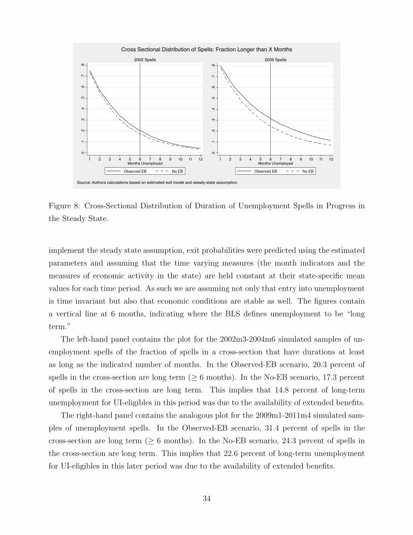
0.1

.2.3

.4.5

.6.7

.8

1 2 3 4 5 6 7 8 9 10 11 12Months Unemployed

Observed EB No EB

2002 Spells

0.1

.2.3

.4.5

.6.7

.8

1 2 3 4 5 6 7 8 9 10 11 12Months Unemployed

Observed EB No EB

2009 Spells

Cross Sectional Distribution of Spells: Fraction Longer than X Months

Source: Authors calculations based on estimated exit model and steady-state assumption.

Figure 8: Cross-Sectional Distribution of Duration of Unemployment Spells in Progress in

the Steady State.

implement the steady state assumption, exit probabilities were predicted using the estimated

parameters and assuming that the time varying measures (the month indicators and the

measures of economic activity in the state) are held constant at their state-specific mean

values for each time period. As such we are assuming not only that entry into unemployment

is time invariant but also that economic conditions are stable as well. The figures contain

a vertical line at 6 months, indicating where the BLS defines unemployment to be “long

term.”

The left-hand panel contains the plot for the 2002m3-2004m6 simulated samples of un-

employment spells of the fraction of spells in a cross-section that have durations at least

as long as the indicated number of months. In the Observed-EB scenario, 20.3 percent of

spells in the cross-section are long term (≥ 6 months). In the No-EB scenario, 17.3 percent

of spells in the cross-section are long term. This implies that 14.8 percent of long-term

unemployment for UI-eligibles in this period was due to the availability of extended benefits.

The right-hand panel contains the analogous plot for the 2009m1-2011m4 simulated sam-

ples of unemployment spells. In the Observed-EB scenario, 31.4 percent of spells in the

cross-section are long term (≥ 6 months). In the No-EB scenario, 24.3 percent of spells in

the cross-section are long term. This implies that 22.6 percent of long-term unemployment

for UI-eligibles in this later period was due to the availability of extended benefits.

34

Note that our steady-state calculation cannot mimic the observed cross-section distribu-

tion of unemployment durations because of the extreme assumptions of constant flows into

unemployment and a stable economic environment. However, this calculation largely recon-

ciles the low survivor rates for individual spells with the relatively high share of long-term

unemployment in total unemployment in the cross-section. In the 2002-2004 period, our

steady-state calculation for the Observed-EB scenario indicates that 17.3 percent of unem-

ployment in the cross-section is long term, compared with a long-term share of 22 percent

based on reported duration in the CPS. In the 2009-2011 period, our steady-state long-term

share is 31.4 percent while the reported CPS long-term share is 39 percent.

The results of these calculations show that a substantial fraction (15-25 percent) of the

long-term unemployment observed in the cross-section is due to the availability of extended

UI benefits.

7 Concluding remarks

We examined the impact of the unprecedented extensions of UI benefits in the United States

over the past few years on unemployment dynamics and duration and compared their effects

with the extension of UI benefits in the milder recession of the early 2000s. We found

small but statistically significant reductions in unemployment exits and small increases in

unemployment durations arising from both sets of UI extensions. The magnitude of these

overall effects is similar across the two episodes.

Potential caveats to our findings include the possible influence of mis-classification of

labor force states leading to mis-measurement of exits from unemployment and the possible

mis-classification of individuals as UI-eligible. The former mis-classification is likely to lead

to a downward bias in our estimated effects of extended benefits. On the other hand, the

results of our placebo analysis of UI-ineligibles raises the possibility that our indicators of

UI availability are correlated with unobserved features of state economic conditions, and

this would lead to an upward bias in our estimated effects of extended benefits. Thus, these

biases likely run in opposite directions and may offset to a greater or lesser extent.

We find that the effect on exit from unemployment occurs primarily through a reduc-

tion in labor force exits rather than through exit to employment (job finding). This is

important because it implies that extended benefits do not delay the time to re-employment

substantially and so do not have large first-order efficiency consequences. The major effect

of extended benefits is redistributive, providing income to job losers who would have exited

35

the labor force otherwise (consistent with Card et al. 2007).

While we find small effects of extended benefits both on exits from unemployment and

on the expected duration of completed unemployment spells, our estimates imply a sub-

stantial effect of extended benefits on the share of unemployment in the cross-section that

is long-term. For example, we find that, during the recent downturn, extended benefits in-

creased the expected duration of unemployment by about 7 percent account but accounted

for about 22 percent of long-term unemployment in the cross-section. This apparent conflict

arises because extended benefits have only small effects on the distribution of unemployment

duration early in spells (≤ 6 months), and the substantial majority of spells end in the first

6 months.

Overall, our estimates suggest that extending unemployment insurance benefits in weak

labor markets has virtually no effect on the rate of job finding but that, on average, unemploy-

ment spells are somewhat longer as a subset of UI recipients remain nominally unemployed

rather than exit the labor force. In addition to these limited implications for economic effi-

ciency, we find only small impacts on the aggregate labor market. We estimate that extended

UI increased the overall unemployment rate by only about 0.4 percentage points in the recent

episode, which is small in comparison with the peak unemployment rate of 10 percent.

36

8 References

Abowd, John M., and Arnold Zellner. 1985. “Estimating Gross Labor-Force Flows.” Journal

of Business and Economic Statistics 3, no. 3: 254-83.

Anderson, Patricia M. and Bruce D. Meyer. 1997. “Unemployment Insurance Takeup Rates

and the After-Tax Value of Benefits.” Quarterly Journal of Economics, 112 (3, Au-

gust): 913-937.

Blank, Rebecca M. and David E. Card. 1991. “Recent Trends in Insured and Uninsured

Unemployment: Is There an Explanation?” Quarterly Journal of Economics, 106 (4,

November): 1157-1189.

Card, David, Raj Chetty, and Andrea Weber. 2007. “The Spike at Benefit Exhaustion:

Leaving the Unemployment System or Starting a New Job?” American Economic

Review, Papers and Proceedings 97: 113-118.

Card, David, and Phillip B. Levine. 2000. “Extended benefits and the duration of UI spells:

evidence from the New Jersey extended benefit program.” Journal of Public Economics

78: 107-138.

Chetty, Raj. 2008. “Moral Hazard versus Liquidity and Optimal Unemployment Insurance.”

Journal of Political Economy 116(2, April): 173-234.

Elsby, Michael, Bart Hobijn, Aysegul Sahin, and Robert G. Valletta. 2011. ”The Labor

Market in the Great Recession: An Update.” Brookings Papers on Economic Activity

103 (Fall), pp. 353-71.

Farber, Henry S. 2010. “Job Loss and Unemployment in the 21st Century: The Great

Recession in Labor Market Perspective.” Working Paper, Industrial Relations Section,

Princeton University, December.

Fujita, Shigeru. 2010a. “Economic Effects of the Unemployment Insurance Benefit.” Federal

Reserve Bank of Philadelphia Business Review, Fourth Quarter.

Fujita, Shigeru. 2010b. “Effects of the UI Benefit Extensions: Evidence from the Monthly

CPS.” Working Paper No. 10-35, Federal Reserve Bank of Philadelphia, November.

37

Howell, David R. and Bert M. Azizoglu. 2011. “Unemployment Benefits and Work Incen-

tives: The U.S. Labor Market in the Great Recession.” Manuscript, The New School,

May (forthcoming in Oxford Review of Economic Policy).

Jurajda, S. and F.J. Tannery. 2003. “Unemployment Durations and Extended Unemploy-

ment Benefits in Local Labour Markets.” Industrial and Labor Relations Review 56(2):

324- 348.

Katz, Lawrence. 2010. “Long-Term Unemployment in the Great Recession.” Testimony to

the Joint Economic Committee, U.S. Congress. April 29, 2010.

Katz, Lawrence, and Bruce Meyer. 1990. “The Impact of the Potential Duration of Unem-

ployment Benefits on the Duration of Unemployment.” Journal of Public Economics

41 (Feb.): 45-72.

Kroft, Kory, and Matthew J. Notowidigdo. 2011. “Should Unemployment Insurance Vary

with the Local Unemployment Rate? Theory and Evidence.” Working paper No.

17173, National Bureau of Economic Research, June 2011.

Landais, Camille, Pascal Michaillat, and Emmanuel Saez. 2010. “Optimal Unemployment

Insurance over the Business Cycle.” NBER Working Paper 16526, November. Cam-

bridge, MA: National Bureau of Economic Research.

Levine, Phillip B. 1993. “Spillover Effects Between the Insured and Uninsured Unemployed,”

Industrial and Labor Relations Review 47: 73-86.

Mazumder, Bhashkar. 2011. “How did unemployment insurance extensions affect the un-

employment rate in 2008-10?” Chicago Fed Letter 285, April.

Meyer, Bruce. 1990. “Unemployment Insurance and Unemployment Spells.” Econometrica

58 (July): 757-782.

Moffitt, Robert. 1985. “Unemployment Insurance and the Distribution of Unemployment

Spells.” Journal of Econometrics 28: 85-101.

Poterba, James M., and Lawrence H. Summers. 1986. “Reporting Errors and Labor Market

Dynamics.” Econometrica 54, no. 6: 1319-38.

38

Poterba, James M., and Lawrence H. Summers. 1995. “Unemployment Benefits and Labor

Market Transitions: A Multinomial Logit Model with Errors in Classification.” Review

of Economics and Statistics 77, no. 2: 207-16.

Rothstein, Jesse. 2011. “Unemployment Insurance and Job Search in the Great Recession,”

Brookings Papers on Economic Activity (Fall): 143-96

OECD. 2007. Benefits and Wages 2007: OECD Indicators (Paris: OECD).

Valletta, Robert G., and Katherine Kuang (2010). “Extended Unemployment and UI Ben-

efits,” FRBSF Economic Letter 2010-12.

Vroman, Wayne. 2010. “The Role of Unemployment Insurance As an Automatic Stabilizer

During a Recession.” Report, Urban Institute and IMPAQ International, July.

Whittaker, Julie M. 2008. “Extending Unemployment Compensation Benefits During Re-

cessions.” Report RL34340, Congressional Research Service, December.

Whittaker, Julie M., and Katelin P. Isaacs. 2012. “Unemployment Insurance: Programs

and Benefits.” Report RL33362, Congressional Research Service, April.

39

Appendix I – The Timing and Extent of Unemployment

Insurance Extensions

The temporary UI extensions initiated in 2008 were historically unprecedented. In addition

to the automatic extensions under the EB program (up to 20 weeks) in 2008, four additional

extensions took effect between mid-2008 and late 2009, as specified by the Emergency Un-

employment Compensation (EUC) program. The initial extension in mid-2008 provided for

13 additional weeks of UI benefits in all states. This was followed by implementation of a

second tier (tier II) in late 2008 that allowed receipt up to 33 weeks of extended benefits,

with eligibility for weeks 21-33 predicated on a state total unemployment rate (TUR) of at

least 6 percent or an insured unemployment rate (IUR, based on the number of regular UI

claimants) of at least 4 percent.

EUC Tiers III and IV were added in early November of 2009. At that point, Tier

II eligibility was expanded by 1 week to 14, and the unemployment rate threshold was

eliminated for Tier II eligibility and applied to Tier III eligibility (13 weeks). Tier IV

eligibility (6 weeks) was based on a TUR of at least 8.5 percent or an IUR of at least 6

percent.23 As of November of 2009 and continuing through early 2012, individuals in states

that met eligibility requirements for EB and all EUC tiers could receive up to 99 weeks of

UI payments (26 weeks of regular benefits, 20 weeks of EB, and 53 weeks of EUC). The

maximum of 99 weeks through existing legislation continued into early September 2012. By

that point, however, many states had ”triggered off” (i.e., became ineligible for) available

EUC tiers and EB benefits based on declines in their unemployment rates. In addition, as

of early September 2012, the number of weeks available through the various EUC tiers was

reduced slightly, lowering the maximum number of UI weeks available from 99 to 93. By

the end of 2012, no state qualified for all EUC tiers and maximum EB benefits; the highest

number of weeks available through all programs in any state at that point was 83.

It is important to note that the EUC program was subject to several temporary suspen-

sions arising from legislative disagreements that precluded seamless reauthorization of the

program. Suspensions of 12 days or longer occurred during April, June-July, and December

of 2010. Although otherwise eligible individuals were unable to apply for a new tier of EUC

23 The EUC triggers also are based on a 10 percent increase in the unemployment rate over the preceding2 years. This constraint has become binding on a widespread basis as labor market weakness persisted. Asof late 2010, the legislation was changed so that the unemployment rate 3 years earlier was used; some stateschose to opt out of the higher tiers subsequent to that change.

40

benefits during those months, these individuals were permitted to attain the new tier after

program reinstatement and receive retroactive benefits. Because reinstatement was expected

and individuals were allowed to receive benefits on their existing tiers during the suspensions,

it is likely that the suspension periods did not significantly offset any behavioral responses

to the overall extension programs. In all of our analyses, we record UI availability during

the EUC suspension months as being identical to availability in the month immediately pre-

ceding the suspension, under the assumption that job search behavior was not affected by

the suspensions.

A similar but much more limited extension of UI benefits occurred through the Tempo-

rary Extension of Unemployment Compensation (TEUC) legislation that was effective from

March 2002 through early 2004. In all states, individuals who exhausted their regular state

UI benefits were automatically eligible for an additional 13 weeks of benefits. Individuals

in states classified as ”high unemployment” (based on the level and change in the insured

unemploymente rate) were eligible for an additional 13 weeks of UI benefits. In conjunction

with EB eligibility of up to 20 weeks, a maximum of 46 weeks of extended benefits and 72

weeks of total benefits were available during the period of TEUC authorization. The TEUC

program was phased out in early 2004, with individuals who filed a valid TEUC claim prior

to the end of 2003 able to continue receiving those benefits for as long as they lasted in 2004

(up to 13 weeks, so potentially through March).

41