Do �Broken Windows� Matter? Identifying Dynamic

Spillovers in Criminal Behavior

Gregorio Caetano & Vikram Maheshri∗

October 4, 2012

Abstract

The �Broken Windows� theory of crime predicts that the incidence of low intensity crimes

in a neighborhood leads to future increases in both the frequency of the same type of crime

(within-crime dynamic spillovers) and the severity of crimes that are committed (across-crime

dynamic spillovers in the direction of increasing severity). We test these predictions using a

detailed database comprised of every crime report �led with the Dallas Police Department

from 2000-2007. Notably, we isolate the intertemporal causal e�ect of crime that is outside of

the control of law enforcement from the total reduced-form causal e�ect of previous crimes on

future crimes, which includes the future police response to previous crimes. Our identi�cation

strategy, based on an �upside-down� regression discontinuity approach, explicitly accounts for

the facts that many determinants of crime are unobservable and that crime data su�ers from

non-classical measurement error. We �nd robust support for the existence of within-crime

dynamic spillovers for robberies, burglaries, auto thefts and light crimes, but little support

for the existence of across-crime dynamic spillovers, particularly in the direction of increasing

severity. Importantly, we �nd no evidence that reductions in light crime a�ect future crimes of

any other type. These results cast considerable doubt on the claim that the dramatic reduction

in the violent crime rate in US urban areas over the past �fteen years is due to �broken windows�

based law enforcement policies. Policymakers aiming to decrease the prevalence of severe crimes

ought to implement policies narrowly targeted to severe crimes. JEL Codes: K42 , R23

1 Introduction

Economic models of crime are built upon the notion that would-be criminals consider the ben-

e�ts of committing crime, the probability of arrest and the potential costs of punishment when

making decisions (Becker (1968)). In a static model, individual- and neighborhood-level hetero-

geneity in both the expected costs and bene�ts of committing various crimes along with agents'

beliefs regarding these costs and bene�ts imply an equilibrium in which crime levels vary across

neighborhoods and by di�erent types of crimes (e.g., Fender (1999)). If, however, the expected costs

∗Departments of Economics, University of Rochester and University of Houston. We thank Carolina Caetano,David Card, Aimee Chin, Frederico Finan, Willa Friedman, Justin McCrary and Noam Yuchtman for valuablediscussions. All errors are our own.

1

and bene�ts of crime are determined in part by the past histories of criminal behavior in di�erent

neighborhoods, then crime must be understood as a dynamic phenomenon.

The leading theory that argues for the existence of intertemporal links in criminal behavior is

the �Broken Windows� theory (BWT) of crime (Kelling and Coles (1998)).1 BWT is developed

around a dynamic mechanism by which the proliferation of less severe crimes (e.g., broken windows

or gra�ti) signals to potential criminals that enforcement, and hence punishment, is lax in the

area. This leads to future crimes of increasing frequency and severity, each one signaling further

to future potential criminals that enforcement is lax. Put di�erently, signals transmitted among

potential criminals lead to herding behavior (Banerjee (1992)).2 Accordingly, BWT carries a strong

policy implication that addressing less severe crimes can be an e�ective means to reduce the rates

of more severe crimes indirectly (Kelling and Sousa (2001)). Indeed, BWT has heavily in�uenced

law enforcement policy in a number of US cities in the past twenty years, notably New York City,

Los Angeles and Chicago.3

In this paper, we provide the �rst causal, empirical test of two implications of BWT: (1) current

crimes of a given type in a neighborhood cause future crimes of that type in that neighborhood (dy-

namic spillovers exist �within crimes�), and (2) higher levels of less severe crimes in a neighborhood

cause higher levels of more severe crimes in the future in that neighborhood (dynamic spillovers

exist �across crimes� in the direction of increasing severity). These two implications are not only

the most important components of BWT; they are necessary conditions for any policy based on the

aggressive targeting of light crime in order to address violent crime rates indirectly.

Any test of these implications must acknowledge three key properties of the intertemporal

relationships between crimes. First and foremost, although discussions about BWT focus mainly

on the social channels through which past crimes may cause future crimes, we argue that the relevant

distinction between intertemporal causal mechanisms of crime is behavioral versus policy based. The

behavioral intertemporal relationship between crime levels fully characterizes the dynamic process

of criminality and includes the social links proposed in Kelling and Coles (1998) (e.g., social learning

and herding behavior) in addition to individual learning mechanisms (e.g. learning by doing), and

any endogenous response to prior crimes that is outside of the control of law enforcement (e.g.,

formation of neighborhood watches by private residents). In contrast, policy based dynamic crime

spillovers include the future responses of law enforcement agencies to changes in past crime levels.

Typically, a policymaker considers a new law enforcement policy that lasts for several periods (weeks

in our case). The main thrust of BWT is that in each period, the indirect e�ects of this policy on

future crimes through behavioral channels must also be considered in addition to the direct e�ects

of future policy interventions. Hence, the goal of this paper is to identify these indirect e�ects

independently of changes in future law enforcement policy. In order to do so, we must therefore

1James Q. Wilson is regarded as one of the originators of this theory (see Kelling, George L. and James Q. Wilson,�Broken Windows,� The Atlantic Monthly, March 1982.)

2Other dynamic models of crime focus on the relationships between criminal decisions and the labor market (Davis(1988); Imai and Krishna (2004)), income inequality and crime (Fajnzlber et al. (2002)) and social networks andcrime (Calvo-Armengol and Zenou (2004)). Glaeser et al. (1996) present a model of crime based on social interactionsbetween criminals to explain geographic variation in crime rates.

3In a 2003 interview with the Academy of Achievement, former New York mayor Rudy Giuliani remarked, �I verymuch subscribe to the "Broken Windows" theory... The idea of it is that you had to pay attention to small things,otherwise they would get out of control and become much worse.�

2

identify only those dynamic spillovers that arise from behavioral sources. Second, social learning

in crime is a local phenomenon, as social distance is likely to be strongly correlated with physical

distance. It follows that an analysis of intertemporal behavioral relationships in crime must proceed

at the neighborhood level as opposed to the city, county or national level. And third, social learning

may occur over short time scales, hence high frequency data is required to identify the full dynamic

spillovers in criminal behavior. We explore these three points in detail.

We start from the notion that any suitable empirical analysis of the dynamic relationship be-

tween crimes must acknowledge that crime data are unlikely to be observed in long run equilibrium

but rather along some trajectory. Given this concern, we conduct our analysis in two stages. In

the �rst stage, we estimate equations of motion for each type of crime, which summarize the co-

evolution of all types of crimes over time. These equations describe the current levels of each type

of crime as causal functions of the previous levels of all types of crime as well as other determinants

of crime. In the second stage, we use the estimated equations of motion to simulate the impulse

responses of crime reduction, i.e., the long run e�ects of reductions in the present level of a given

crime on the future levels of all crimes holding all else constant. These simulations allow us to test

for the existence of within-crime and across-crime dynamic spillovers in criminal behavior and to

assess their importance quantitatively.

We face three main obstacles in consistently estimating the equations of motion. First, unob-

served determinants of future crimes may be correlated to previous crime levels (e.g., if they are

serially correlated). Second, we as researchers observe only reported crimes as opposed to actual

crimes, and the associated measurement error in crime data may not be classical (Skogan (1974),

Skogan (1975)). Third, the standard method to deal with these two problems � the use of instru-

mental variables � is unsuitable to test the implications of BWT because it will necessarily identify

the total reduced-form e�ect of previous crimes on future crime, which includes the intertemporal

e�ect of crimes through induced changes in future police actions. To identify only the behavioral

causal link, we must control for observable and unobservable changes in future police actions.

To deal with these issues, we leverage an extremely rich dataset to implement a novel identi�-

cation strategy based on Caetano (2012) which we call the �upside-down� regression discontinuity

(UD-RD) approach. Brie�y, we take a selection on observables approach and specify successively

richer sets of control variables to account for potential endogeneity. The novelty of our identi�cation

strategy stems from the fact that we can explicitly test the selection on observables hypothesis using

the discontinuity test developed in Caetano (2012). Speci�cally, we conduct a statistical test of the

ability of our control variables to absorb endogeneity from a number of sources related to omitted

variables, measurement error and unobserved future police actions. This test can be understood

as an �upside-down� regression discontinuity test because it is based on identifying assumptions

that are the inverse of the identifying assumptions used in a standard regression discontinuity (RD)

approach. In an RD approach, the main explanatory variable in the equation of interest varies dis-

continuously at some threshold value, and researchers assume that unobservables vary continuously

at that threshold. A discontinuity in the dependent variable at the threshold is therefore inter-

preted as evidence that the main explanatory variable is included in the equation, i.e., it causes the

dependent variable (Imbens and Lemieux (2008); Lee (2008)). Analogously, in our setting, the main

3

explanatory variables in our equations of motion vary continuously at a threshold, and we assume

that the unobservables correlated to these variables vary discontinuously at that threshold. If the

dependent variable varies discontinuously at the threshold conditional on a set of control variables,

then this constitutes evidence that these unobservables are included in the equation, i.e., there are

endogeneity concerns in our speci�cation. If, however, the dependent variable varies continuously

at the threshold conditional on a set of control variables, then we cannot reject exogeneity of our

main explanatory variables.

To develop our UD-RD approach, we argue theoretically that unobserved determinants of crime,

measurement error and unobserved future police actions are each likely to be discontinuous where

the level of previously reported crime equals to zero. Our argument is based on the idea that since

reported crime levels cannot be negative, any determinant of previously reported crimes (or any

variable that is correlated to any such determinant) will generally be discontinuous at zero due to a

bunching of observations. We support our theoretical argument by showing empirically that a wide

variety of observed determinants of crime, including variables related to (mis)reporting of crimes

and future police actions, are indeed discontinuous at the zero threshold, which constitutes indirect

evidence that unobserved determinants of crime are also discontinuous.4 We then proceed to select

a speci�cation in which we �nd no discontinuities in the causal relationships between all types of

previous crimes and future crimes. Importantly, this test of exogeneity is agnostic to the source of

potential endogeneity, which could arise from unobserved future police responses, from (classical or

non-classical) measurement error in crime reports or from other unobserved determinants of crime

in the neighborhood. We supplement our identi�cation strategy with a variety of conventional

robustness checks, all of which support the notion that our preferred estimates under the UD-RD

approach are indeed consistent.

Although there is a large empirical literature that explores determinants of crimes and geographic

variation in criminal activities (e.g., Gould et al. (2002); Levitt (2004)), few have attempted to

analyze directly the dynamic relationship among di�erent types of crimes. Funk and Kugler (2003)

�nd mild evidence in favor of positive across-crime dynamic spillovers in national crime rates of

larceny, burglary and robbery in Switzerland. Several studies have attempted to evaluate the

success of BWT based policing by estimating the relationship between misdemeanor arrests and

the prevalence of violent crimes. Implicit in these studies is the idea that misdemeanor arrests

directly translate into reductions in low intensity crime. Hence, an examination of the relationship

between misdemeanor arrests and the prevalence of violent crime can be thought of as a test

for dynamic spillovers from low intensity crimes to high intensity crimes by proxy. Corman and

Mocan (2005) analyze BWT based policing in New York City by estimating the impact of city-

wide misdemeanor arrests on more severe crimes and �nd that robberies, motor vehicle thefts and

grand larcenies are most a�ected by such enforcement strategies. Skogan (1992) argues that low

grade disorder is a primary determinant of further serious crime with the use of crime victimization

surveys in 30 neighborhoods across six US cities. However, an alternative analysis of this data by

Harcourt (1998) suggests this claim is sensitive to missing data and statistical outliers. None of

4This argument is analogous to the one used in RD approaches in which observables that are shown to varycontinuously at the threshold constitute indirect evidence that unobservables vary continuously at the threshold.

4

these aforementioned studies attempt to account systematically for omitted determinants of crime,

unobserved future police responses and potential endogeneity stemming from measurement errors,

so it is di�cult to interpret their results as causal. Jacob et al. (2007) use weather shocks as

instruments and �nd a small negative within-crime intertemporal relationship. However, they focus

on the full temporal displacement of crime as opposed to the induced criminal behavioral due to

prior crime that underlies BWT, as they do not distinguish between behavioral and policy based

intertemporal links between crimes, and their analysis is conducted at the city level. Harcourt

and Ludwig (2006) take advantage of a random allocation of public housing under the �Moving to

Opportunity� experiment in �ve US cities and �nd no e�ect of neighborhood misdemeanor crime

levels on the propensity to commit violent crime of those who were assigned to that neighborhood.

Braga and Bond (2008) randomize police e�orts to reduce social disorder in certain neighborhoods

of Lowell, Massachusetts and �nd that increased policing reduces citizen calls for service for more

severe crimes, though measurement error in citizen reporting may be a source of concern. Finally,

Keizer et al. (2008) provide evidence from �eld experiments that is consistent with the behavioral

mechanism at the core of BWT by showing that when individuals observe violations of social norms,

they are more likely to violate these norms themselves.

We conduct our analysis using a unique, comprehensive database containing every police report

�led with the Dallas Police Department from 2000-2007. In total, this database contains reports of

nearly 2 million unique crimes. Each police report contains detailed information regarding the type,

location and time of the alleged crime. In addition, each police report contains information regarding

the speed and quality of the police response to the crime. We use this database to construct a panel

data set containing the weekly levels of six types of crimes (rape, robbery, burglary, motor vehicle

theft, assault and light crime) in every Dallas neighborhood. A key feature of our data set is the

high frequency at which it is constructed. By performing our analysis at the weekly level, we are

able to estimate the immediate intertemporal e�ects of previously committed crimes. This allows us

to test for the existence of dynamic spillovers in criminal behavior directly instead of using annual

misdemeanor arrests as a proxy for changes in light crimes. Importantly, we �nd that the e�ects of

previous crimes on future crimes dissipate entirely after four weeks, which highlights an advantage

of our data set over the lower frequency data sets used in previous analyses of BWT. In spite

of this high sampling frequency, the considerable cross-sectional variation in our data set enables

us to estimate economically insigni�cant intertemporal e�ects that are nevertheless statistically

signi�cant.

We �nd that a reduction of one robbery or light crime (e.g., gra�ti) leads to an additional

cumulative future reduction of roughly 0.1 crimes of the same type. A reduction of one auto

theft leads to an additional cumulative future reduction of 0.2 auto thefts, and a reduction of

one burglary leads to an additional cumulative future reduction of 0.4 burglaries. We do not �nd

any economically signi�cant within-crime dynamic spillovers in rapes or assaults. Although we

�nd that unit reductions in assaults lead to future reductions of nearly 0.005 rapes and 0.025

robberies, we �nd no statistically signi�cant evidence of other dynamic spillovers across crimes of

increasing severity. Importantly, reductions in the levels of light crimes are not found to generate

economically or statistically signi�cant reductions in the future levels of more severe crimes. These

5

results constitute support for the �rst implication of BWT but no support for the second � and more

policy relevant � implication of BWT. We interpret our �ndings as casting considerable doubt on the

claim that the dramatic reduction in the crime rate (especially the violent crime rate) in US urban

areas over the past �fteen years is due to broken windows law enforcement policy.5 Our �ndings

suggest that law enforcement agencies aiming to reduce violent crimes should pursue policies that

are narrowly tailored to combat those crimes.

We also �nd that unit reductions of robbery, auto theft and assaults generate spillover reductions

of 0.18, 0.10 and 0.05 light crimes respectively. These across-crime spillovers are of the same order

of magnitude as the within crime spillovers associated with light crime, suggesting that a policy

that targets more severe crimes will generate spillover bene�ts that strictly dominate the spillover

bene�ts of a policy that targets light crime. We acknowledge that even if a �broken windows� law

enforcement policy is ine�ective at reducing violent crime rates, it may still be an optimal policy

from a cost-bene�t perspective. In an extension of our analysis, we perform a back of the envelope

calculation using social cost-of-crime estimates from Heaton (2010) and Miller et al. (1993) and

calculate that unless the marginal cost of reducing robbery (burglary) is more than 25 (7) times

greater than the marginal cost of reducing light crime, then a broken windows law enforcement

policy is inadvisable on cost-bene�t grounds.

The remainder of the paper is organized as follows. In section 2, we describe our strategy to

identify intertemporal relationships between neighborhood crimes. In section 3, we describe our

data set and argue for the validity of our identi�cation strategy. In section 4, we present estimates

of the equations of motion for crime, and in section 5 we show that those estimates withstand a

variety of conventional robustness checks. In section 6 we calculate dynamic spillovers in criminal

behavior by simulation to test the two empirical implications of BWT, and we use these results

to perform a back of the envelope cost-bene�t analysis of various law enforcement policies. We

conclude in section 7.

2 Identi�cation Strategy

Crime today may cause crime in the future through several channels that can be categorized

as either behavioral or policy based. Behavioral channels include any endogenous intertemporal

responses to current crimes. For example, herding behavior by criminals (Banerjee (1992)), learning-

by-doing or specialization in criminal activity (Kempf (1987)), incapacitation (Levitt (1998)) and

neighborhood responses to crime (Taylor (1996)) are all classi�ed as behavioral. Policy based

channels include any future police response to current crimes that a�ects future crime levels. For

example, a police crackdown or a change in the distribution of police resources due to an increase

in the number of crimes (Sherman and Weisburd (1995)) are classi�ed as policy based.

From the perspective of a policy maker, it is crucial to distinguish between these two channels.

In order to evaluate a particular investment to combat crime today, it is necessary to know both the

short-run and the long-run e�ects of this investment holding constant any additional investments

5Levitt (2004) describes e�orts by the media to attribute falling crime rates in New York City to innovative lawenforcement policies, including �broken windows� style policies, but he argues that this conclusion is premature givenother confounding changes that occurred in New York City at the same time or even before a �broken windows�policy was implemented.

6

that will be made to combat crime in the future. Suppose, for example, that a policy was available

that would eliminate a single robbery in a neighborhood today. Other things equal, if this policy

resulted in fewer robberies committed tomorrow than expected, then we would rightly interpret

this as a dynamic spillover. If instead this policy resulted in the same number of robberies commit-

ted tomorrow as expected in the absence of the policy, but fewer law enforcement resources were

deployed tomorrow, then we should also interpret this as a policy relevant dynamic spillover. This

example underscores the need to hold the level of future law enforcement resources constant. By

doing so, we assume that police resources are as productive after a policy intervention as before. In

practice, this hypothetical crime reduction policy might potentially take the form of a reallocation

of police resources today, e.g., the deployment of additional police in places where robberies are

suspected to occur. Note, however, that this is consistent with holding �xed the deployment of

police resources tomorrow.6

We now formalize our empirical approach to identify these dynamic spillovers. Let x?cjt denote

the number of crimes of type c committed in neighborhood j in week t. We collect the levels of

all crimes into the row vector X?jt ≡

(x?1jt . . . x

?Cjt

), where the crime types are ordered by decreasing

severity. The equation of motion for crime of type c in neighborhood j in week t can be written as

x?cjt = X?jt−1β

c + Zcjtγc + P cjt + εcjt︸ ︷︷ ︸

error

. (1)

where Zcjt is a vector of all observed determinants of x?cjt that are not behavioral responses to crime,

which includes characteristics of previous crimes, �xed e�ects and observed police responses to

previous crimes. P cjt includes all unobserved police responses to past crimes. εcjt is an error term,

which includes other unobserved determinants of crime as well as misspeci�cation error.

2.1 Identi�cation Issues

In equation (1), βc can be interpreted as the behavioral component of the intertemporal e�ect of

crime because it excludes the e�ects of X?jt−1 on x?cjt through Zcjt and P cjt. Given estimates of

βc for all crimes c, the long-run dynamic spillovers associated with crime can be computed via

a straightforward simulation procedure, which we describe in section 6. However, we face three

distinct obstacles to identify βc:

1. As researchers, we are only able to observe reported crime levelsXjt, whereXjt ≡(x1jt, . . . , x

Cjt

),

for all c. Accordingly, we rewrite equation (1) as

xcjt = Xjt−1βc + Zcjtγ

c + P cjt + ηcjt + εcjt︸ ︷︷ ︸error

(2)

6We also choose to hold the future response of police �xed in order to withstand the Lucas critique (Lucas (1976)).BWT based policies are not likely to be implemented for only one period (week), and the manner in which policerespond to previous crimes under these policies may di�er from the manner in which police respond to previouscrimes in the observed data. If we do not hold the police response �xed, then we e�ectively assume that the policewill allocate their resources next period as a function of crimes today in the same manner as they did when our datawas sampled, i.e., before implementing a BWT policy. Thus, holding the police response �xed in the data providesa more relevant benchmark.

7

where the additional term ηcjt is the error induced by mismeasurement of the crime variables

in both the left hand side and the right hand side of the equation. If ηcjt is correlated to

Xjt−1, then our estimates will be biased.7

2. εcjt is likely correlated to Xjt−1. This endogeneity arises if εcjt is serially correlated since εcjt−1causes Xjt−1 trivially. Indeed, most unobserved neighborhood amenities that determine crime

are likely to possess this property.

3. Estimation with instrumental variables (IVs), which is the typical approach to deal with the

two issues above, will be unable to identify behavioral dynamic spillovers. Instead, IVs will

identify the full reduced-form e�ect ofXjt−1 on xcjt, which includes the component through the

future unobserved police response P cjt. Put di�erently, the behavioral e�ect is not identi�ed

by instrumental variables because any candidate IV that generates variation in Xjt−1 (i.e.,

is relevant) will also generate variation in P cjt (i.e., is invalid). For intuition, we graphically

depict the inability of an IV to address the endogeneity due to P cjt in diagram (3).

Zcjt

γc

IV // Xjt−1 βc //

""

xcjt

P cjt

>>

(3)

Because of the timing of events, P cjt is caused by Xjt−1, which induces a correlation between

a potential instrument and P cjt as denoted by the dotted line. Unless we are able to fully

control for P cjt (in which case the instrument is super�uous), the instrument will be invalid.

2.2 The �Upside-Down� Regression Discontinuity Approach

In light of these di�culties, we pursue an alternative strategy to identify βc in equation (2). Un-

derlying our identi�cation strategy is the fact that we observe a very rich set of control variables,

Zcjt, which allows us to take a selection on observables approach. What is novel about our ap-

proach is that we can explicitly test the selection on observables hypothesis using an �upside-down�

regression discontinuity (UD-RD) test (Caetano (2012)). Given a method of testing the selection

on observables hypothesis, we can enrich the set of included control variables until we no longer

reject exogeneity8 of our main explanatory variables (i.e., we cannot reject that βc is consistently

estimated) at a suitably low con�dence level.9 We �rst discuss our identi�cation strategy in greater

7Although there is a large literature in criminology on the mismeasurement of reported crimes (see Skogan (1974)and Skogan (1975) for a seminal treatment on the topic), we do not explore the particulars of the data generatingprocess for these errors because our identi�cation strategy is agnostic to this mechanism.

8As we proceed through our empirical analysis, we provide ample evidence that our preferred speci�cations arenot �hand picked� among several rejected speci�cations. For instance, we show that when we take a speci�cation forwhich we cannot reject exogeneity and we add more control variables, we continue not rejecting exogeneity.

9Importantly, we argue in section 4 that the control variables in our preferred speci�cations do not absorb thebehavioral intertemporal e�ects of crime that we want to measure.

8

detail and then discuss its implementation.

The UD-RD test is so named because its identifying assumptions are the inverse of the identifying

assumptions in the standard regression discontinuity (RD) approach. As such, we develop the

intuition behind our identi�cation strategy by analogy to an RD approach. In the standard RD

framework, identi�cation arises from the assumption that all unobservable determinants of the

outcome vary continuously at some threshold value of the running variable (top panel of �gure 1)

and the fact that the main explanatory variable varies discontinuously at that threshold (bottom

panel of �gure 1). Any discontinuity in the outcome variable at the threshold can therefore be

taken as evidence that the main explanatory variable is a causal determinant of the outcome, i.e.,

it is included in the equation to be estimated. In contrast, identi�cation in our setting arises from

the assumption that some unobservable variable varies discontinuously at the threshold (top panel

of �gure 2) and the fact that the main explanatory variable of interest varies continuously at the

threshold (bottom panel of �gure 2).10 Any discontinuity in the outcome variable at the threshold

is therefore taken as evidence that the unobservable variable should be included as a determinant

of the outcome, i.e., there is endogeneity in the equation to be estimated.11

In a UD-RD framework, the running variable is the main explanatory variable itself, so continuity

of the explanatory variable with respect to the running variable is trivially satis�ed. Moreover,

unobservables that vary discontinuously at the threshold are correlated with the main explanatory

variable by construction. It follows that a discontinuity of the outcome variable at the threshold

conditional on control variables is evidence that these control variables are unable to absorb enough

omitted variables, i.e., the estimate of the e�ect of the main explanatory variable on the outcome

is likely biased. Conversely, the absence of a discontinuity in the outcome variable at the threshold

conditional on control variables is evidence that these control variables are able to absorb enough

omitted variables, i.e., the estimate of the e�ect of the main explanatory variable on the outcome

is likely unbiased.

Furthermore, in the standard RD framework, it is not possible to provide fully dispositive

evidence for the identifying assumption that unobservables vary continuously at the threshold. To

do so would require researchers to show that all unobservable determinants of the outcome vary

continuously at the threshold. In practice, researchers show that many observable determinants of

the outcome vary continuously at the threshold, which provides indirect evidence that unobservable

determinants also vary continuously at the threshold. Similarly, in the UD-RD framework, it

is not possible to provide fully dispositive evidence for the identifying assumption that at least

10In this paper, we explore the discontinuity in unobservables at a boundary point, which may look odd incomparison to standard RD approaches, where the threshold usually lies at an interior point. Note, however, that anRD approach can be implemented with a discontinuity at a boundary point as long as the RD identifying assumptionof continuity of unobservables is valid at that point. In practice, it is usually di�cult to argue that the identifyingassumption in an RD approach is valid at a boundary point, exactly because the UD-RD identifying assumption ofdiscontinuity of the unobservables is often valid at boundary points.

11In practice, the outcome may be a discontinuous function of the main explanatory variable at the threshold evenif the main explanatory variable varies continuously at the threshold. In this paper, we rule this possibility out byassuming that the equations of motion are linear. An analogous assumption is made in the standard RD framework.Showing that an observed covariate varies continuously at the threshold, as is typically done in the RD approach,does not preclude it from having a discontinuous e�ect on the outcome, as the outcome may still be a discontinuousfunction of this covariate at the threshold. Similarly, this possibility is usually ruled out by a linearity assumption(or more generally by a continuity assumption).

9

one unobservable varies discontinuously at the threshold. In practice, we show that a variety

of observable determinants of the outcome variable vary discontinuously at the threshold, which

similarly provides indirect evidence that unobservable determinants also vary discontinuously at

the threshold.

2.3 Implementation

Equation (2) can be rewritten as

xcjt = Xjt−1βc + Zcjtγ

c + qcjtλc + µcjt︸ ︷︷ ︸

P cjt+η

cjt+ε

cjt

, (4)

by gathering the three potential sources of endogeneity in the equations of motion. The total error

component in equation (4) is split into two terms: qcjt, which is correlated with Xjt−1 (conditional

on Zcjt), and µcjt, which is an exogenous error term. Our goal is to design a test for the hypotheses

H0 : λc = ~0 for all c

H1 : λc 6= ~0 for some c

where ~0 is a zero vector. For a given speci�cation of the equations of motion, rejecting the null

hypothesis constitutes evidence that our speci�cation su�ers from endogeneity. On the other hand,

not rejecting the null hypothesis constitutes evidence that the controls in that speci�cation capably

address endogeneity concerns.12

To ensure that our test has power, we make the following identifying assumption:

Assumption 1. qcjt is discontinuous in xc′

jt−1 at xc′

jt−1 = 0 for some c, c′.

For each speci�cation of the equations of motion, assumption 1 provides an independent way

of testing the ability of our control variables to absorb any potentially confounding variation in

crime levels that is unobserved. Under this assumption, if we �nd that conditional on Zcjt, xcjt

varies discontinuously with Xjt−1 at xc′

jt−1 = 0 for any c and c′, then it must be the case that

some element of λc is di�erent from zero for some c. This implies that we must reject the null

hypothesis. If, however, we �nd that xcjt varies continuously at xc′

jt−1 = 0 for all c and c′, then we

can conclude that all elements of λc are equal to zero for all c, which implies that we cannot reject

the null hypothesis. Intuitively, the power of this test � and hence our con�dence in the consistency

of our estimates if we cannot reject the null hypothesis of exogeneity � is increasing in the number

of discontinuous unobservables and the sizes of their discontinuities.

12Altonji et al. (2005) describe a di�erent approach to measure the importance of qcjt relative to total explanatorypower of Xjt−1 and Zc

jt. In particular, they o�er a method to compute the ratio of the amount of selectionon unobservables relative to the amount of selection on observables that would be required to exist if the entireestimated e�ect was fully attributed to endogeneity. In addition to di�erent primitive assumptions, the notabledistinction between their approach and ours is that we are able to test the selection on observables hypothesis itself.Hence, we can make statements of the form, �we cannot reject exogeneity of Xjt−1 at the α̂ level of signi�cance�where α̂ is the critical size of the test that we can directly estimate.

10

Implementation of this test requires only a simple parametric modi�cation to the equations of

motion. De�ne the row vector of dummy variables Djt−1 ≡(d1jt−1, . . . , d

Cjt−1

)as follows

dcjt−1 = 1 if xcjt−1 = 0 (5)

= 0 otherwise

We modify equation (2) to

xcjt = Xjt−1βc + Zcjtγ

c +Djt−1δc + ucit (6)

where δc is a C × 1 vector of parameters to be estimated, and ucit is an error term. If each element

of δ1, . . . , δC is equal to zero, then Xjt−1 does not a�ect xcjt discontinuously at xc′

jt−1 = 0 for all

c, c′. To test formally for whether all elements of δ1, . . . , δC are equal to zero, we use a joint F-test.

For each speci�cation, the F-test provides statistical evidence for the (non)existence of at least one

variable that is wrongly omitted from the speci�cation among all unobserved variables that vary

discontinuously at xc′

jt−1 = 0 for some c′. If it is the case that all wrongly omitted variables vary

discontinuously in xc′

jt−1 for some c′, then this test has power against all sources of endogeneity.

In the following section, we argue empirically and theoretically that unobservable determinants

of crime, measurement error and unobserved police responses to prior crimes all vary discontinuously

with xc′

jt−1 at xc′

jt−1 = 0 for some c′. This constitutes indirect evidence that these three sources of

endogeneity all satisfy assumption 1; that is, this constitutes indirect evidence that the UD-RD test

has power against these three sources of endogeneity. We then estimate various speci�cations of the

equations of motion, each with an increasingly rich set of control variables. For each speci�cation, we

test for endogeneity from unobservable determinants of crime, measurement error and unobserved

police responses using the UD-RD test. To the extent that there are other unobservables that are

correlated with our main explanatory variables (i.e., elements of qcjt that do not satisfy assumption

1), our test will not have power against all sources of endogeneity. Because of that, we supplement

the UD-RD test with a variety of conventional robustness checks.

3 Data and Preliminaries

3.1 Sample

We assemble a database encompassing every crime that was reported to the Dallas Police Depart-

ment from January 1, 2000 to September 31, 2007.13 According to the FBI, Dallas held the dubious

distinction of having the highest crime rate of all US metropolitan areas with at least one million

persons during the sample period.14 This database is uniquely suited to test the implications of

BWT because it includes a comprehensive catalog of all light crimes of various types that were

reported. During our sample period, the Dallas Police Department was geographically organized

13A small number of crime reports � sexual o�enses involving minors and violent crimes for which the complainant(not necessarily the victim) is a minor � are omitted from our data set for legal reasons.

14�New York Remains Safest Big City in US,� September 19, 2006, The Associated Press.

11

into six divisions, subdivided into 32 sectors which were further subdivided into police beats.15

Beats range from roughly 0.5 to two square miles in area, and each sector contains �ve to seven

beats and one police station.

Every report in our database lists the exact location (address or city block) of the crime and

is given a �ve digit Uniform Crime Reporting (UCR) classi�cation by the responding o�cer.16 A

full description of the complainant who called in the report is also provided, with the exception of

anonymous reports. Private companies and public o�cials/o�ces may be listed as complainants.

Every report also lists a series of times from which we can deduce the entire sequence of crime,

neighborhood response and police response. Speci�cally, we observe the time (or estimate of the

time) that the crime was committed, the time at which the police were noti�ed and dispatched,

the time at which the police arrived at the scene of the crime, and the time at which the police

departed the scene of the crime.

We perform our analysis on six crimes: rape, robbery, burglary, motor vehicle theft, assault

and light crime. Because of potential misclassi�cation, we de�ne assault as both aggravated and

simple assault (Zimring (1998)). We classify criminal mischief, drunk and disorderly conduct,

vice (prostitution), fence (trade in stolen goods) and found property (almost exclusively cars and

weapons) as light crimes. 17 We select this set of crimes for four reasons. First, this set of crimes

includes both violent crimes and property crimes of varying levels of severity, which allows us to

test for across-crime dynamic spillovers. Second, these crimes are likely to signal criminals' actual

beliefs of the strength of enforcement to potential criminals, which forms the basis of the social

learning mechanism suggested by BWT. In contrast, crimes such as embezzlement and gambling

are less publicly observable. Third, these crimes occur relatively more frequently than other publicly

observable crimes such as homicide and arson. And fourth, these crimes are relatively accurately

reported in comparison with crimes such as larceny and fraud.18

We provide summary statistics for these reported crimes in table 1. Not surprisingly, light crime

is the most prevalent crime reported, followed by assault, burglary, auto theft, robbery and rape.

Police respond to crimes in approximately 80 minutes on average, although they respond to reports

of rape roughly an hour slower and to reports of motor vehicle theft roughly half an hour faster.

On average, police spend less than half an hour at the scene of a motor vehicle theft, but they

spend up to an hour at the scenes of robberies and light crimes and over an hour at the scenes of

reported rapes. All types of crimes occur slightly more frequently on weekends than weekdays with

the exception of burglaries, which happen less frequently on weekends than weekdays. Just over

half of robberies, light crimes and motor vehicle thefts occur at night, and as expected, a majority of

15In October 2007, DPD added a seventh division to their classi�cation and made slight modi�cations to somebeat and sector boundaries. We end our sample in September 2007 to ensure that the beats and sectors in our dataset are geographically consistent over the entire sample period.

16If a particular complaint consists of multiple crimes (e.g., criminal trespass leading to burglary), then the reportis classi�ed only under the most severe crime (burglary) per UCR hierarchy rules developed by the FBI.

17As added robustness checks, we replicated our full analysis de�ning only criminal mischief and found propertyas light crime, or alternatively de�ning criminal mischief only as light crime. In all three cases, we obtained similarresults.

18The accuracy of reported rape statistics is admittedly poor (Mosher et al. (2010)). To the extent that the

propensity to misreport rape varies discontinuously at xc′

jt−1 = 0 for some c′, our test of exogeneity will also test formismeasurement in rape levels. As an added robustness check, we replicated our full analysis excluding rapes andobtained similar results.

12

these crimes take place outdoors. On the other hand, burglaries and assaults tend to occur during

the daytime and indoors. Rapes tend to occur at night and indoors. Private businesses report

approximate one �fth of robberies and light crimes and one third of burglaries, but they report very

few motor vehicle thefts and no rapes or assaults.

Although we observe each crime individually, the relevant variables in our model are levels of

crime in pre-de�ned neighborhoods and time periods. As such, we aggregate crimes geographically

by sector and temporally by week. We choose to de�ne neighborhoods as sectors rather than beats

in order to internalize the information spillovers from observed crime levels in neighboring beats.

This de�nition still preserves substantial heterogeneity in crime rates across neighborhoods in a

given time period. By performing a weekly analysis, we ensure that we have a long time series (402

periods) with su�cient intertemporal variation in crime levels within neighborhoods. We discuss

in detail the empirical implications of our aggregation choices in section 5.3.

3.2 Empirical Support for Assumption 1

By analogy to the RD approach, we provide indirect empirical evidence in support of assumption

1 in the form of discontinuity plots (�gure 3). Each point in these plots represents the mean

of the variable on the y-axis (some other potential determinant of current crime levels, such as

another element of Xjt−1 or an element of Zcjt−1 for some c) conditional on a given level of xc′

jt−1

for some c′. The dashed curve represents a third order local polynomial regression of all of these

points for which xc′

jt−1 > 0, and the shaded region represents the 95% con�dence region for this

regression, with an out of sample prediction at xc′

jt−1 = 0.19 Finally, the hollow point represents

the observed mean value of the variable on the y-axis conditional on xc′

jt−1 = 0. If the hollow

point lies outside of the shaded region, then this implies that the observed variable on the y-axis

is discontinuous at xc′

jt−1 = 0 with at least 95% con�dence, which is indirect evidence in support

of the validity of assumption 1. Indeed, we show that there is ample evidence of discontinuities for

various potential determinants of xcjt.20 Although we cannot formally assess why the discontinuities

arise in each �gure, our identi�cation strategy only requires that they exist, irrespective of their

sources. Nevertheless, we o�er suggestive explanations for these discontinuities with the intention

of providing intuition for our identi�cation strategy.21

In panels 3a and 3b we plot the shares of various reported crimes that occur on the weekend

against reported crime levels in the same week. In the �rst panel, we �nd that assaults occur

discontinuously more frequently on weekends in weeks without reported burglaries, and in the

19For each regression, we use the Epanechnikov kernel with bandwidths of �ve for the kernel and the standarderror calculation.

20To be sure, our running variables, xc′

jt−1, are discrete. Given the fact that they take on a wide variety of values,

we approximate them to be continuous in order to test for discontinuities in the values of other variables at xc′

jt−1 = 0.

This approach of using a discrete running variable is also common in RD studies (e.g., Lee and McCrary (2005),Card et al. (2008)).

21In our sample there are no observations with zero units of light crime, so we cannot search for discontinuities in

unobservables at xlight crimet−1 = 0. However, our test still has power against unobservables correlated to light crime

to the extent that they are also correlated to other crimes for which we do �nd discontinuities (see, for example,panels 3c, 3f, 3h, 3i and 3k.)

13

second panel, we �nd that robberies occur discontinuously less frequently on weekends in weeks

without reported auto thefts. Similarly, in panels 3c and 3d we plot the shares of various reported

crimes that occur during the daytime against reported crime levels in the same week. We �nd that

light crimes and rapes occur discontinuously more frequently during the daytime in weeks without

reported auto thefts and burglaries respectively. All four of these discontinuities could re�ect

di�erent levels of within-week intertemporal substitutibility between these various types of crimes.

In panels 3e and 3f, we �nd analogous discontinuities in the shares of assaults and light crimes that

occur outdoors against reported robberies and burglaries respectively. These discontinuities could

re�ect di�erent levels of within-neighborhood spatial substitutibility between these various types of

crimes. The discontinuities found in panels 3a-3f suggest that our UD-RD approach has the power

to test against misspeci�cation related to temporal and spatial aggregation.

In panels 3g-3j we plot the average police response time to reports of various crimes in week

t against reported crime levels in week t − 1. In the �rst two panels, we �nd that police respond

discontinuously faster to burglaries and light crimes after weeks in which no auto thefts are reported.

This discontinuity may arise because police shift their attention away from auto thefts and towards

other property crimes.22 In panel 3i we �nd that police respond discontinuously slower to light

crimes after weeks in which no burglaries are reported, and in panel 3j, we �nd that police spend

discontinuously less time at the scenes of reported rapes after weeks in which no auto thefts are

reported. In all four cases, we �nd indirect evidence that P cjt varies discontinuously with some

explanatory variables of interest. These results suggest that our UD-RD approach has power to

test against endogenous changes in future police actions.

In panel 3k we plot the share of light crimes that are reported by private businesses in week

t − 1 against reported burglaries in week t − 1, and in panel 3l we plot the share of auto thefts

reported by public employees in week t− 1 against reported robberies in week t− 1. In both cases,

we �nd that when no burglaries and robberies are reported, the share of light crimes reported by

private businesses and the share of auto thefts reported by public employees are discontinuously

lower, respectively. This may re�ect the propensity of non-individuals to under report less severe

property crimes when more severe property crimes are absent. These discontinuities in reporting

behavior suggest that our UD-RD approach has power to test against measurement error in crime

data.

In totality, these discontinuity plots illustrate the variety of sources of endogeneity that we have

power to test against.

3.3 Theoretical Support for Assumption 1

Admittedly, �gure 3 is not an exhaustive catalog of discontinuous potential determinants of crime.

Even though we are unable to provide dispositive explanations for the sources of these discontinu-

ities, we can o�er a general theoretical argument for how these discontinuities � and many others

� are likely to arise in our data. Fundamental to this argument is the fact that reported crimes

22In the case of light crimes (panel 3h), it may be that a discontinuously higher number of light crimes last week(see panel 3c) causes the police to pay more attention to these crimes the following week.

14

are truncated at zero; that is, there cannot be a negative number of reported crimes in any neigh-

borhood. In general, this truncation will generate bunching of latent variables at the threshold of

xc′

jt−1 = 0. To develop this argument and connect it to our application, we separately consider each

of the three sources of potential endogeneity discussed earlier (unobserved determinants of crime,

measurement error, and the response of police to past crime) and o�er additional theoretical argu-

ments for why omitted endogenous variables of these types will vary discontinuously at xc′

jt−1 = 0

for some c′.

Figure 4 illustrates a hypothetical relationship between a generic explanatory variable, xc′

jt−1,

and a particular unobservable determinant of past crime, e.g., the average neighborhood wealth in

period t−1, which is included in εcjt−1. From the �rst panel of the �gure, poorer neighborhoods are

expected to have higher levels of reported crime, but in wealthier neighborhoods reported crime is

expected to be lower. When the level of wealth is ε?, no crimes are reported in expectation. For any

neighborhood with an average wealth larger than ε?, the expected level of reported crime will still

be 0, as it cannot be negative. Conversely, we can plot the expected value of neighborhood wealth

for each level of reported crime, as in the second panel of the �gure. Here, we �nd a mechanically

generated discontinuity in expected wealth when no crimes are reported: neighborhoods with no

reported crimes include not only those with εcjt−1 = ε? but also those with εcjt−1 > ε?. Intuitively,

there are neighborhoods that are so wealthy that even if they were slightly poorer, no crimes would

be reported in expectation.

As another example, we illustrate the relationship between xc′

jt−1 and the propensity of neigh-

borhood residents to misreport crime in period t − 1 in �gure 5. When a crime occurs, residents

decide whether or not to report it to the police, hence this variable is the main determinant of

measurement error. If poorer neighborhoods are more distrustful of law enforcement, or if prop-

erty crimes committed in poorer neighborhoods are of lower value, then there would be greater

misreporting in poor neighborhoods than in richer neighborhoods (Skogan (1977)). In conjunction

with the previous example, this suggests that the propensity to misreport crime may be positively

correlated with the level of reported crime. In the �rst panel of �gure 5, neighborhoods that are

more likely to misreport crime are shown to su�er from higher expected levels of reported crime.

When the propensity to misreport is low enough (i.e., ηcjt = η?), no crimes are reported in expec-

tation. For any neighborhood with a lower propensity to misreport than η?, the expected reported

level of crime will still be zero. This implies a discontinuity in the conditional expectation of the

unobservable at the level of reported crime equals to 0, as shown in the second panel. Intuitively,

in some neighborhoods nearly every crime that is committed is reported, and even if a few people

began to harbor distrust of the police, the lack of actual crime in the neighborhood would still lead

to no crimes being reported.

We add three remarks about the generality of the argument illustrated by these two examples.

First, because we have an extensive panel data set, our unit of observation is a neighborhood-week

pair, instead of merely a neighborhood. Any bunching of observations (as opposed to bunching of

neighborhoods) at xc′

jt−1 = 0 for some c′ will generate a discontinuity similar to the one described

in assumption 1. For instance, if a particular neighborhood has a high level of some unobserved

amenity in the �rst week of every month (say, because of a monthly farmer's market), then this

15

unobservable amenity will vary discontinuously at xc′

jt−1 = 0 for some c′. Second, the relationship

between the unobservable and xc′

jt−1 need not be monotonic as illustrated in these �gures, nor does

the discontinuity need to lie in the direction of the slope of xc′

jt−1 near xc′

jt−1 = 0. Finally, a su�cient

(but not necessary) condition for assumption 1 to hold is that qcjt is caused by some unobservable

that causes xc′

jt−1.23 This guarantees that the bunching of observations with no reported crime

(xc′

jt−1 = 0) will generate a discontinuity in qcjt in expectation.24

Following the logic of the examples above, the police response to past crimes, P cjt, may be

discontinuous at xc′

jt−1 = 0 if it is caused by P cjt−1. Indeed, a police presence may a�ect the

reporting of crime directly by deterrence or indirectly by mitigating measurement error, so any

inertia in the allocation of police resources would imply a discontinuity in P cjt at xc′

jt−1 = 0. In

fact, the police response may be discontinuous for a second reason: P cjt itself may be caused by

Xjt−1 discontinuously at xc′

jt−1 = 0. Consider for instance the level of attention that the police give

to a neighborhood. Prior reported crimes may cause a change in this unobservable (e.g., due to a

police crackdown). Hence, we would expect a positive relationship between xc′

jt−1 for some c′ and

the unobservable police response P cjt, as illustrated in �gure 6. When fewer crimes are reported,

the police tend to reduce their attention in the following period.25 Because the police observe only

reported crimes as opposed to actual crimes, the response of the police to prior reported crimes

could be discontinuously di�erent when there is no crime reported versus when there is one crime

reported simply because the lack of reported crime in a neighborhood may leave it �under the radar�

for that week.26

4 Estimation Results

We estimate β1, . . . , βC from the following system of equations

x1jt = Xjt−1β1 + Z1

jtγ1 +D1δ1 + u1it

... (7)

xCjt = Xjt−1βC + ZCjtγ

C +DCδC + uCit ,

23In �gure 4, εcjt−1 is not included in qcjt. However, qcjt contains ε

cjt, so any serial correlation in neighbors' wealth

will generate a discontinuity in qcjt.24The only instance in which assumption 1 does not hold is if qcjt is a discontinuous function of the unobservable at

precisely the point at which that unobservable causes xc′

jt−1 = 0 (denoted as ε? and η? in �gures 4 and 5, respectively)and that the size of this discontinuity exactly o�sets the original discontinuity of the unobservable.

25There may also be a substitution e�ect as resources are re-allocated to prevent other types of crime. In thiscase, we may observe a negative relationship between prior reported crime and policing for c 6= c′. Nevertheless, ouridenti�cation strategy is motivated by the existence of this relationship, not by its sign.

26The intertemporal behavioral e�ect of crime is less likely to be discontinuous in Xjt−1 at xc′

jt−1 = 0 for all c′

for two reasons. First, the intertemporal behavioral e�ect is a particular function of X?jt−1 that is distinct from

Xjt−1 since private individuals do not necessarily observe what is reported to the police. Second, di�erent privateindividuals are likely to have heterogeneous knowledge about previous crimes within the same neighborhood (someindividuals may observe more and others may observe fewer actual crimes than the police). It follows that the

aggregate actions of private individuals at xc′

jt−1 = 0 (i.e., when each of them observes whatever they observe in

weeks when the police observe xc′

jt−1 = 0) is unlikely to di�er much from their actions at xc′

jt−1 = 1, for each c′. Asa practical matter, we show in section 4 that this argument turns out to be super�uous, as we are unable to rejectthe null hypothesis of exogeneity even when only control variables that absorb non-behavioral e�ects are included inour preferred speci�cations.

16

which represent the equations of motion of all crimes. Given that our data forms an extensive

panel, our controls largely (but not exclusively) take the form of various �xed e�ects. The evi-

dence in support of assumption 1 ensures that the test which underlies our identi�cation strategy

has statistical power. We present six sets of coe�cient estimates for various speci�cations of our

equations of motion for all crimes in table 2. In each speci�cation, the system of equations (7) is

estimated e�ciently by seemingly unrelated regression (Zellner (1962)) with di�erent sets of con-

trols. Given that the primary source of bias is likely the omitted determinants of crime that are

positively serially correlated, e.g., neighborhood amenities, we would expect our naive estimates of

βc to be biased upward in speci�cations with insu�cient controls.

In speci�cation 1, we do not include any control variables. We �nd that an additional reported

crime of any type (except for rape) adds approximately half of a reported crime of that type in the

next week. On the other hand, we �nd that an additional reported rape decreases half of a reported

rape in the following week. Moreover, we �nd that additional reported crimes of any type increase

reported crime levels of all types in the following week, although the across-crime intertemporal

e�ects are an order of magnitude smaller than the within-crime intertemporal e�ects. Almost all

coe�cients are precisely estimated at the 99% level with the exception of the coe�cients on rape,

and we are able to explain 81% of the variation in reported weekly neighborhood crime levels with

this speci�cation. However, the joint F-statistic is large, which indicates that at least one element

of δc for at least one c is statistically distinguishable from zero at the 99% signi�cance level. This

implies that at least one of the Xjt−1 a�ects one of the xcjt discontinuously at xc′

jt = 0, hence we

must reject consistency of our estimates of βc in this speci�cation.

In speci�cation 2, we add year-crime type �xed e�ects as control variables. These variables

absorb any annually varying determinants of each type of crime. Previous attempts to identify in-

tertemporal relationships between crimes (Funk and Kugler (2003)) and between crime and policing

(Corman and Mocan (2005)) are based on speci�cations similar to this, as they utilize only low-

frequency control variables such as annual unemployment rates, which are absorbed by the �xed

e�ects. The coe�cient estimates with this speci�cation are roughly similar to our estimates from

speci�cation 1. Indeed the increase in R2 of 0.002 from speci�cations 1 to 2 indicate that these

slowly varying control variables explain little additional variation in weekly neighborhood crime

rates. In addition, the joint F-statistic is still large, implying that we must again reject consistency

of our estimates of βc. This �nding casts doubt on the results of earlier empirical tests of BWT.

In speci�cation 3, we add sector-crime type �xed e�ects and week-crime type �xed e�ects as

control variables. These variables absorb any omitted neighborhood speci�c determinants of each

crime and any omitted city-wide week speci�c determinants of each crime respectively. Overall the

coe�cient estimates are precisely estimated, but decrease in magnitude relative to speci�cations

1 and 2, which con�rms our conjecture that these omitted variables are positively correlated with

criminal activity. With the inclusion of these �xed e�ects, we are able to explain 85% of the variation

in reported weekly neighborhood crime levels. Based on the large joint F-statistic, we again reject

consistency of our estimates of βc, this time at the 95% con�dence level.27 This indicates that

27Because this speci�cation is marginally rejected, we are hesitant to make strong inference based solely on theF-test. When we look at the estimates of the elements of δ1, . . . , δC individually, we �nd that 3 out of 30 of them

17

this set of control variables is insu�cient to absorb endogenous variation in the unobservables, and

hence it could be misleading to interpret the βc estimated in speci�cation 3 as causal estimates of

the intertemporal behavioral e�ects of crime.

In speci�cation 4, we enrich the set of control variables by disaggregating the �xed e�ects

by sector-year-crime type and division-week-crime type. The �rst set of �xed e�ects absorbs all

omitted neighborhood speci�c determinants of each crime that vary on an annual basis (e.g., any

redistribution of police resources across sectors).28 The second set of �xed e�ects absorbs all time

varying determinants of each crime that vary across the six police divisions that divide Dallas. To

the extent that unobservables in di�erent neighborhoods are serially correlated, these �xed e�ects

would absorb the unobservables that are common to all neighborhoods within each division. In

short, the only potential omitted variable that could bias our estimates would have to vary across

weeks within a calendar year and across sectors within a division. As in the previous speci�cations

all coe�cients are precisely estimated, with the exception of the rape coe�cients, whose standard

errors are relatively large due to the lack of variation in the levels of rape. With the exception of

rape, we estimate statistically signi�cant within-crime type intertemporal e�ects of less than half

of the magnitude of the e�ects estimated in speci�cation 3. We �nd less evidence for across-crime

intertemporal e�ects, although we do �nd some positive e�ects at the 95% con�dence level, mostly

at the direction of decreasing severity.29 In particular, we �nd no evidence that light crime has any

intertemporal e�ects on more severe crimes. With these �xed e�ects, we are able to explain 87%

of the variation in reported weekly neighborhood crime levels. Importantly, the joint-F statistic is

su�ciently small that we do not reject consistency of the βc estimates at even as high a signi�cance

level as 60%, well above the standard critical levels. This suggests that the inclusion of the higher

order year-sector and division-weekly �xed e�ects successfully addresses potential endogeneity in

our estimation of the equations of motion of crime.

5 Additional Robustness Checks

In the last section we used the UD-RD approach to provide evidence in favor of the estimates in

speci�cation 4 and against the estimates in speci�cations 1, 2 and 3. In this section, we leverage the

richness of our dataset to conduct a series of additional robustness checks to argue that our estimates

of βc in speci�cation 4 are indeed unbiased by omitted variables, spatial and serial autocorrelation

of errors and misspeci�cation due to aggregation.

are statistically signi�cantly di�erent from zero at the 99% level At this level of statistical signi�cance, we wouldexpect to reject 0.3 of the coe�cients at random. Based on these facts, we reject exogeneity of our main explanatoryvariables. For comparison, in speci�cations 4-6, no estimates of the elements of δ1, . . . , δC are statistically signi�cantat the 99% level, suggesting that the additional control variables successfully deal with endogeneity.

28 Unobservable amenities that are changing over time due to gentri�cation will be partially absorbed by these

�xed e�ects to the extent that they vary across years in the sample.

29Gladwell (2000) has popularized the notion that BWT implies the existence of a �tipping point� level of lightcrime beyond which the levels of light crime and more severe crimes are on an ever increasing trajectory. Our �ndingsthat within- and across-crime intertemporal e�ects are much less than one are inconsistent with this view.

18

5.1 Omitted Variables

Although we cannot reject exogeneity of speci�cation 4 in table 2, we conduct further robustness

tests of our estimates by including additional controls related to the timing and location of crimes

and to the response of police to past crimes. In speci�cation 5, we enrich our set of control

variables by including the shares of each type of crime reported to have been committed in the

daytime and on the weekend in the previous week and the shares of each type of crime reported

to have been committed outdoors in the previous week. This allows us to explore if either our

temporal or spatial aggregation of observations introduces endogeneity into our speci�cation. If

crimes committed during the daytime (outdoor) generate di�erent intertemporal e�ects than crimes

committed at night time (indoor), then speci�cation 4 would be misspeci�ed, which might bias our

parameter estimates. Based on our �nding that some observed (yet omitted) variables related

to the aggregation of observations are discontinuous (�gure 3), the low joint F-statistic found

in speci�cation 4 implies that our estimates of βc should nonetheless be consistent. Indeed, we

�nd almost no change in either the coe�cient estimates, the joint F-statistic, or the R2 between

speci�cations 4 and 5.

In speci�cation 6 we provide further evidence in support of the claim that βc can be interpreted

as the intertemporal behavioral e�ect of crime. Here, we expand the set of control variables from

speci�cation 5 by adding, for each type of crime, the average time that the police take to arrive at

the crime scene in the current week, and the average duration that police remain at the crime scene

in the current week.30 These variables proxy for the level of attention of the police for each type of

crime in that neighborhood in the current week. The inclusion of these variables have no e�ect on

the estimates of βc, nor do they explain any additional variation in reported weekly neighborhood

crime levels. Indeed, we are unable to reject the hypotheses that all police response and police

duration coe�cients are equal to zero even at the 66% level of signi�cance. We interpret this as

evidence that our �xed e�ects successfully absorb unobserved determinants of police responsiveness,

which is con�rmed by the low joint F-statistic.

We supplement these results with a dynamic robustness check for our estimates of βc by allowing

reported crimes from earlier periods (e.g., t−2, t−3, . . . , t−T ) to a�ect crime in period t. Formally,

we modify the system of equations of motion of crime to

x1jt =

T∑k=1

(Xjt−kβ

1k + Z1

jt−k+1γ1k +D1

kδ1k

)+ u1it

... (8)

xCjt =

T∑k=1

(Xjt−kβ

Ck + ZCjt−k+1γ

Ck +DC

k δCk

)+ uCit

for values of T = 1, . . . , 4. We re-estimate these systems of equations using the full set of available

control variables from speci�cation 6 in table 2 and present coe�cient estimates for βc1 (the coe�-

30Given the system of 6 equations of motion each with 6 main explanatory variables, we e�ectively add 36 averagepolice response and 36 average police duration variables as controls.

19

cient vector for Xjt−1) in table 3. To the extent that the inclusion of these variables do not change

our estimates of βc1, only omitted variables that are uncorrelated with earlier levels of crimes can

generate endogeneity in our speci�cation. It is immediate that our estimates of βc1 in speci�cations

with higher order lags (i.e., columns 2 through 4) are statistically indistinguishable from our prior

estimates, which are reproduced in the �rst column. As xcjt−k for k = 2, ..., 4 are each very likely to

be correlated to xcjt−1 for all c, the fact that the estimates of xcjt−1 do not change with the inclusion

of these additional lags constitutes further evidence that the βc coe�cients in speci�cation 4 in

table 2 are consistent.31

As we add more lagged explanatory variables, the joint F-test includes more coe�cients.32 For

instance, for the speci�cation with 4 lags, we test whether all elements of δck are equal to zero, for

all c and k = 1, ..., 4. This happens because the inclusion of more lags allows for the possibility to

test for discontinuities at xc′

jt−k = 0 for k = 1, ..., T , which increases the power of the test. We are

unable to reject the consistency of the estimates of βck for any of these speci�cations at the 10%

signi�cance level.33 For brevity, we omit the large number of coe�cients on higher order lagged

terms in speci�cations with T = 2 and T = 3, but we present a full set of coe�cient estimates

for our preferred speci�cation with T = 4 in table 4. As before, across-crime intertemporal e�ects

in the direction of increasing severity are precisely estimated, but small and overall statistically

insigni�cant. Notably, for any lag we can rule out that a unit increase in light crime will increase any

other type of crime by 0.034 or more units at the 95% con�dence level. Within-crime intertemporal

e�ects are precisely estimated, but successively smaller in size for higher lags, being statistically

signi�cant mostly up until the third lag. Note that our �ndings of higher order within-crime

intertemporal e�ects do not contradict the consistency of the estimates of βc1 found in column 1

of table 3. That is, from an estimation standpoint, a speci�cation of the equations of motion of

crime with a single lag is valid. However, when computing dynamic spillovers in the next section,

we would like to allow for all intertemporal causal e�ects, even at higher lags.

We remark that the control variables included in our preferred speci�cations do not absorb the

intertemporal behavioral response to prior crimes that we want to include in our estimates of βckfor two reasons. First, as long as behavioral intertemporal e�ects persist for less than one year,

the sector-year-crime type �xed e�ects will not absorb them. Indeed, we �nd that these e�ects last

less than four weeks. Second, as long as behavioral intertemporal e�ects are transmitted within

sectors (neighborhoods) only, and not also across sectors within divisions, the division-week-crime

31Because we have no theoretical basis for choosing a maximum value of T = 4, we also estimate the equation ofmotions with T = 5 and T = 6. We are unable to reject exogeneity of both speci�cations at 20% signi�cance level.Moreover, we cannot reject joint F-tests of the null hypotheses that all elements of βc

5 equal zero and all elementsof βc

6 equal zero at the 75% and 40% signi�cance levels respectively. Accordingly, we choose T = 4 as our preferredspeci�cation.

32As we add more lagged explanatory variables, we also include more controls for the proportion of crimes thatwere committed at daytime, on weekends and outdoor, as they all enter the regression for each lag and for each typeof crime.

33Because accepting the null hypothesis of exogeneity at the 10% signi�cance level might be interpreted as onlymarginally insigni�cant, we are hesitant to make strong inference based solely on the F-test. When we inspect theestimates of Dc

k individually for the speci�cation with up to four lags of each explanatory variable, we �nd that only

1 out of 120 estimates (an element of δrobbery3 ) is statistically signi�cantly di�erent from zero at the 99% level. Giventhat by chance we would expect to �nd 1 out of 100 signi�cant estimates at the 1% level, we interpret this result asrobust evidence that there are no omitted endogenous variables in that speci�cation.

20

type �xed e�ects will not absorb them. Even if there is a common behavioral intertemporal e�ect

across sectors within a division, this is likely to be of second order importance in comparison to

the e�ect within the sector. As such, we are con�dent that our estimates of βck exclude only those

intertemporal channels that are policy based.34

5.2 Non-Classical Measurement Error

Unobservable determinants of crime may su�er from two non-classical properties, spatial autocor-

relation and serial correlation, that could bias our inference. Although the inclusion of division-

week-crime type and sector-year-crime type �xed e�ects likely absorb these irregularities, we can

also exploit the considerable longitudinal and cross sectional variation in our panel dataset to check

for the presence of these sources of biases using alternative approaches.

Determinants of crime are potentially spatially autocorrelated across neighboring regions (e.g.,

Moreno� and Sampson (1997)) for two reasons. First, the levels of unobserved amenities of a

particular neighborhood that determine local crime rates may be correlated with the levels of those

amenities in nearby neighborhoods, generating positive spatial autocorrelation. Second, crime

in one neighborhood may displace crime from nearby neighborhoods, generating negative spatial

autocorrelation (Cornish and Clarke (1987)). If determinants of crime are spatially autocorrelated,

then our estimates βc may be biased due to endogeneity, and their standard errors may also be

biased, a�ecting inference.

In section 4 we address the endogeneity issue with the UD-RD approach and by adding �xed

e�ects at the division-week-crime type to absorb any unobservable determinant of crime that is

common across neighboring sectors. If the endogeneity problem is addressed by the control vari-

ables in our preferred speci�cations, then we would expect that the errors in such speci�cations

would be spatially uncorrelated. As an alternative check, we re-estimate the equations of motion

and cluster the standard errors at a larger geographic level than our panel: by division-year-crime

type as opposed to by sector-year-crime type (e.g., Dube et al. (2010)). By doing so, we allow ujt

to be correlated with uj′t, where j and j′ are neighborhoods within the same division of Dallas. In

table 5, we reproduce all standard errors from all speci�cations of the equations of motion presented

in table 2 in bold. Directly below these standard errors in normal font, we present all standard

errors clustered at the division-year-crime type. Two features of the standard errors are immediate.

First, the original standard errors clustered by sector-year-crime type di�er substantially from the

standard errors clustered by division-year-crime type in speci�cations 1-3. Second, the standard

errors clustered by division-year-crime type are nearly identical to the standard errors clustered by

sector-year-crime type in speci�cations 4-6; that is, in these speci�cations any previously estimated

statistically signi�cant intertemporal e�ect remains statistically signi�cant under the broader clus-

tering, and vice versa. These �ndings taken together suggest that the additional control variables in

34Apart from �xed e�ects, the only controls from the current week are police response variables. Because theircoe�cients are all statistically insigni�cant, we conclude that they do not absorb any component of the behavioralintertemporal e�ect. In principle, it could be that the police response exactly o�sets the behavioral intertemporale�ect, rendering the observed response variables insigni�cant. However, this would have to happen simultaneouslyfor all 72 such variables for us to accept the null hypothesis that the coe�cients on the response variables are jointlystatistically insigni�cant.

21

our preferred speci�cations e�ectively absorb potential spatial autocorrelation in the errors, while

the control variables in speci�cations 1-3, which are rejected by the discontinuity F-test, do not.

This provides further independent evidence in favor of our identi�cation strategy.

Determinants of crime may also be serially correlated (Fajnzylber et al. (2002)), which has

two implications for our empirical analysis. First, serially correlated errors may be a source of

endogeneity, hence our estimates of βc might be biased. Second, positively serially correlated errors

may make inference misleading, as standard errors may be too small. In section 4 we address

the �rst issue with our UD-RD approach through the addition of sector-year-crime type �xed

e�ects. Moreover, we show in section 5.1 that the introduction of higher order lagged terms into

the regression does not a�ect the estimates of βc1. We address the second issue by clustering our

standard errors at the sector-year-type of crime. This allows unobserved determinants of crime

within a given sector in a particular week to be correlated with unobserved determinants of crime

within that sector across all other weeks in the same year (Angrist and Pischke (2009)). If the

endogeneity problem is addressed by the control variables in our preferred speci�cations, then we

would expect that the errors in these speci�cations are serially uncorrelated. In order to check this,

we re-estimate the equations of motion under all speci�cations and cluster the standard errors by

week-division-crime type instead of by year-sector-crime type. These standard errors are presented

in italics in table 5. Given that in speci�cations 4-6 the standard errors clustered at the year-

division-crime type level are similar to the ones clustered at the year-sector-crime type level from our

test of spatial correlation, we can use these standard errors to infer the extent of serial correlation in

the remaining error. Analogous to the case of spatial autocorrelation, we �nd that in speci�cations

4-6 the two sets of standard errors are nearly identical. We conclude that the control variables in

speci�cations 4-6 e�ectively deal with any serial correlation in the errors.

5.3 Misspeci�cation Due to Aggregation

We aggregate reported crimes by week and by sector in order to specify the equations of motion

of crime. In doing so, we assume that the data generating process is such that crimes committed

at di�erent times within a week and in di�erent locations within a neighborhood a�ect future

crime levels in identical ways. Although we make these assumptions for explanatory, interpretative

and operational reasons, there is admittedly no clear theoretical basis for them. However, our

extensive data set, coupled with the use of the UD-RD framework o�ers a unique tool to test for

misspeci�cation due to aggregation.

We �rst consider misspeci�cation due to temporal aggregation. We conduct our analysis at

the weekly level in order to have a long panel that possesses su�cient variation in crime levels

within neighborhoods over time. Our robustness checks in section 5.1 assure us that aggregation

at the weekly level is preferable to aggregation at longer time scales. If the data generating process

for reported crimes truly operated at the monthly level, for instance, then we would expect our

coe�cient estimates for the �rst four lags to be equal, i.e., βc1 = βc2 = βc3 = βc4. This is clearly not

the case.

There is still the concern that aggregation at the weekly level is too coarse and that the true data

22

generation process operates at a shorter time scale. Because we observe the exact time that every

crime is reported to occur, we observe crime levels at all levels of temporal aggregation. This allows

us to create variables of the form �share of crimes c committed on the weekend� or �share of crimes

c committed during the daytime� that we observe, which capture within-week variation in crime

levels. To the extent that the time scale is misspeci�ed in our equations of motion, this omitted

variation could bias our estimates of βc. The substantial evidence of discontinuities in variables of

this form that we �nd in panels 3g-3j of �gure 3 ensures that our UD-RD framework has power

to test for the presence of this omitted variation in our speci�cation. The fact that we cannot

reject exogeneity of βc even in speci�cation 4 of table 2, which does not contain these variables

as controls, is evidence that neither these variables nor any ones related to temporal aggregation

that are correlated with these variables are endogenous omitted variables. This point is further

corroborated when we include these variables in speci�cations 5 and 6 and �nd that our estimates

of βc are unchanged and that we cannot reject that the coe�cients on all of these variables are

equal to zero. This suggests that our data are not misaggregated temporally in the sense that if

such misaggregation exists, then it does not generate endogeneity in our preferred speci�cations.

We use a similar argument to show that our data are not misaggregated spatially. Our data are

likely not aggregated at too �ne a geographic level; if the true data generation process operated in-

stead at the division level, then the division-week-crime type �xed e�ects would absorb all variation

in crime levels, and we would estimate all elements of βc to be zero. Further, the UD-RD approach

provides indirect evidence that any error generated because we aggregated the data at a too large

geographical level does not generate endogeneity concerns in our preferred speci�cations. Panels

3k and 3l of �gure 3 show that there are discontinuities in variables of the form �share of crimes c

committed outdoors,� which are related to within-sector geographic variation. Again, the fact that

we cannot reject exogeneity of βc in speci�cation 4 of table 2, which does not contain these variables

as controls, is evidence that neither these variables nor any ones related to spatial aggregation that

are correlated with these variables are endogenous omitted variables. And similarly, inclusion of

these variables in later speci�cations leaves our estimates of βc unchanged, which suggests that our

data are not misaggregated spatially.

6 Computing Dynamic Spillovers of Crime

The coe�cient estimates in table 4 capture the direct e�ects of reported crimes in one week on

all reported crimes in the following 1 to 4 weeks. However, prior crimes may indirectly continue

to a�ect future crimes of all types over a longer time horizon. Any test of the implications of the

BWT must consider the long run e�ects of various crimes, which include the direct and indirect

intertemporal e�ects both within and across crimes.

In order to explore these dynamic interactions, we use our coe�cient estimates to perform an

experiment in which we reduce one reported crime of a given type in week 0 and then simulate

the evolution of all reported crimes in weeks 1, 2, . . . holding all else constant.35 We then compute

the cumulative change in the levels of all crimes relative to how they would have evolved in the

35In particular, we hold constant the current arrest and incarceration policies used by law enforcement.

23

absence of the counterfactual reduction. We interpret the cumulative simulated changes in future

crime levels as the dynamic spillovers that are associated with reductions in current crime levels

holding all else constant except the endogenous behavioral responses to crime.

We begin by presenting simulation results for our test of the �rst implication of BWT, namely

the existence of within-crime dynamic spillovers. In �gure 7, we show the impulse response functions

for counterfactual unit reductions of each crime type. Each panel corresponds to a speci�cation

of the equations of motion for crime with a di�erent number of lags of each explanatory variable.

By comparing the di�erent panels of the �gure, it is clear that the total within-crime spillover

e�ects generally increase as we add more lags to the speci�cation up until T = 3, at which point

they stabilize. Burglaries generate the largest within crime dynamic spillovers, as a reduction of

one burglary abates an additional 0.4 future burglaries. A reduction of one auto thefts results in a

reduction of roughly 0.2 future auto thefts, while unit reductions of robberies and light crimes result

in future reductions of roughly 0.1 additional robberies and light crimes respectively. We identify

only very small within-crime dynamic spillovers for assault and negative within-crime dynamic

spillovers for rape.

In order to test the second implication of BWT, we graph the impulse response functions of

all crimes from unit crime reductions of each type in �gure 8. For brevity, we only present these

impulse response functions using our preferred speci�cation of the equations of motion for crime

with up to four lags of each explanatory variable (T = 4). Six weeks after the unit crime reduction,

nearly all long run spillovers are realized. With this in mind, we calculate cumulative long run

spillovers by letting t→∞ and present them in �gure 9 along with 95% con�dence intervals.36 The

label above each panel refers to the type of crime that we hypothetically reduce by one unit, and

the labels for each bar refer to the type of crime that experiences the spillover. Note that the y-axis

for rapes is at a di�erent scale from the y-axis for the other crimes, since the estimated spillovers

for rapes as an explanatory variable are relatively imprecise. It is immediate that all within-crime

dynamic spillovers are statistically signi�cant, with the exception of assault, and these spillovers

tend to be large relative to across-crime dynamic spillovers, with the exceptions of rape and assault.

We �nd no statistically signi�cant across-crime dynamic spillovers associated with reductions

in light crime, which suggests that a �broken windows� policy will have little success reducing the

levels of severe crimes. For perspective, we note that the spillover bene�ts associated with a policy

that targets either robbery or auto theft strictly dominate the spillover bene�ts of a policy that

targets light crime, as the across-crime e�ects of reducing robbery and auto theft on light crime are

of the same order of magnitude as the within-crime e�ect of reducing light crime. A policy that

targets assaults generates spillover reductions in light crime that are smaller than the within-crime

spillovers associated with light crime reduction, but this policy also generates positive spillover

reductions in rape and robbery levels. However, this policy generates no within-crime spillover.

Even though a policy that targets burglaries does not generate across-crime spillovers, it generates

the largest within-crime positive spillovers of all of the crimes. We are unable to assess the bene�ts

36Because our equations of motion are linear in Xjt−1, . . . , Xjt−T , the cumulative long run spillovers can becomputed analytically. The standard errors for these spillovers are calculated using the delta method, which accountsfor the correlations among the elements of βc

k for all c and k.

24

of a hypothetical policy that targets rapes due to imprecision in our estimates of the dynamic

spillovers associated with such a policy.37

Although �gure 9 o�ers insight into the statistical signi�cance of our results and the trade-o�s

involved in targeting each crime, it is di�cult to glean the economic signi�cance of these dynamic

spillovers. To provide this context, we conduct the following thought experiment. First, we consider

an average neighborhood in an average week of our sample. In this neighborhood, we perform a

hypothetical intervention in which we fully eliminate all crimes of type c for a week and compute the

total cumulative long run spillovers within and across all crimes as t→∞. We then express this long

run dynamic spillover e�ect on crimes as a fraction of the weekly crime level in the neighborhood.

The results of this exercise allow us to construct an upper bound on the e�cacy of a targeted

city-wide intervention. We present the cumulative reductions in crimes from these interventions in

table 6. For example, a complete elimination of light crime in the average neighborhood for one

week (a reduction of 23.15 light crimes) generates a total future spillover reduction in rapes equal

to 9.5% of the average number of weekly rapes in the neighborhood (a cumulative reduction of 0.03

future rapes).

Three results are immediate from table 6. First, within crime spillovers tend to be relatively

large, with the exception of assault, and are precisely estimated. Second, across crime spillovers in

the direction of increasing severity are economically and statistically insigni�cant in all cases with

the exceptions of spillovers from assaults to rapes and robberies, which are marginally statistically

signi�cant. Those two exceptions aside, even a full elimination of lower intensity crimes generates

at most modest spillover reductions in severe crimes (on the order of 5-10%). Notably, eliminating

light crime has a small and statistically insigni�cant impact on other crime rates. Third, across

crime spillovers in the direction of decreasing severity are also statistically insigni�cant, with the

exception of the spillovers on light crime that are generated by reductions of robbery, auto theft

and assault. In sum, these �ndings suggests that a �broken windows� law enforcement policy based

on aggressively targeting light crimes will fail to reduce the rates of more severe crimes in an

economically signi�cant way. Our conclusions are robust and persist under all speci�cations of the

equations of motion for which we cannot reject exogeneity using the UD-RD test.

6.1 Cost-Bene�t Analysis

Even if a �broken windows� law enforcement policy that targets light crimes cannot materially

reduce severe crime rates, it may still be an optimal policy from a cost-bene�ts perspective. We

expand on this point by performing a back of the envelope evaluation of the monetary bene�ts of

various crime reduction policies. In table 7, we present estimates of the monetary bene�ts of a unit

crime reduction. In the �rst column, we list the social costs of one unit of each type of crime that

we adapt from Heaton (2010) and supplement with Miller et al. (1993).38 These estimates of the

social costs of each type of crime are designed to account for both tangible and intangible costs

of crime. Tangible costs include direct �nancial costs to individuals, businesses and governments

37The inclusion of rape in our analysis is important because we are able to precisely estimate the intertemporale�ects of other crimes on rape.

38Details of the construction of these cost estimates can be found in the footnote to table 7.

25

including productivity losses. Intangible costs include losses in quality of life due to fear of crime

and the psychological costs of victimization.

In the second column of table 7, we compute the total monetary bene�ts that are associated with

a law enforcement policy that reduces one unit of a particular type of crime. We calculate these by

simulating the spillover changes in all crimes associated with a unit reduction of a particular type

of crime, valuing them according to the �gures in column 1, and adding them to the direct bene�t

of the unit reduction. For example, a policy that reduces one robbery generates roughly $86,000

in social bene�ts. On the other hand, a �broken windows� law enforcement policy that reduces one

unit of light crime generates only $3,341 in social bene�ts. We caution that these estimated bene�ts

are based on an analysis of only six types of crime; to the extent that reductions in these six crimes

generate dynamic spillovers across other types of crimes (e.g., murder), we will be misestimating

the social bene�ts of crime reduction.

A simple comparison of the bene�ts of crime reduction policies is incomplete without a con-

comitant consideration of the costs of implementing these policies. Unfortunately, we are unable

to �nd estimates of the marginal costs of abating speci�c crimes. Nevertheless, we can still use

our analysis to o�er a rough policy prescription. In the third column of table 7, we present the

bene�ts of unit crime reduction policies in terms of the bene�ts from a unit light crime reduction

policy. Unless the marginal cost of reducing robbery is more than 25.88 times the marginal cost

of reducing light crime, a policy targeting robberies is preferable from a cost-bene�t perspective

to a �broken-windows� law enforcement policy, and unless the marginal cost of reducing burglary

is more than 7.06 times the marginal cost of reducing light crime, a policy targeting burglaries is

preferable to a �broken-windows� law enforcement policy. Similar results for the remaining crimes

are presented in the table.

7 Conclusion

The �Broken Windows� theory of crime has had a large in�uence on urban law enforcement

policy in the past twenty years. Although there has been a vibrant debate over the desirability and

e�cacy of policies based on this theory, the empirical analysis of the fundamental implications of

BWT has been incomplete. In this paper, we o�er the �rst empirical evidence of the (non)existence

of causal intertemporal linkages between criminal behavior which forms the mechanism at the core

of BWT. First, we show that reductions in robberies, burglaries, auto thefts and light crimes of a

given type generate dynamic spillovers by which additional crimes of the same type are eliminated

in the future. Second, we show that reductions in a crime of a given type generate no statistically

or economically signi�cant dynamic spillovers by which additional crimes of higher severity are

eliminated in the future.

The primary policy content of BWT follows from the notion that less severe crimes will en-

dogenously lead to more severe crimes being committed. Under this assumption, a law enforcement

agency utilizing BWT based policing techniques ought to preferentially divert policing attention and

resources from more severe crimes to less severe crimes in order to take advantage of this dynamic

spillover. Our analysis casts substantial doubt on the e�ectiveness of such a policy in abating more

26

severe crimes. Instead, if a city aims to reduce the levels of severe crimes, our analysis supports

law enforcement policies that aggressively and narrowly target severe crimes. Indeed, the evidence

of dynamic spillovers from higher intensity crimes to light crime that we �nd suggests that the

spillover bene�ts of such policies will strictly dominate the spillover bene�ts of a �broken windows�

policy. In a rough cost-bene�t analysis, we �nd that unless the marginal costs of combating severe

crimes exceed the marginal costs of combating light crimes by a factor of at least 25 for robbery

and 7 for burglary, BWT based policing is likely ine�cient.

Our analysis also o�ers a novel application of the �upside-down� regression discontinuity ap-

proach, a methodological tool that is well suited to empirical analyses in the economics of crime. A

central obstacle in the way of identifying the determinants of crime and the e�ects of crime on other

outcomes is the preponderance of non-classical measurement error that has been well documented

in criminal data. In many contexts, UD-RD o�ers an easily implementable, formal test for whether

the available data has been used successfully to mitigate misspeci�cation and measurement errors.

Moreover, in contexts where instrumental variables are unavailable or unable to identify the causal

channel of interest as in our case, this empirical approach may be helpful. Indeed, such contexts

are not limited to the economics of crime.

We conclude by noting that further inquiry into the costs and bene�ts of targeted law enforce-

ment policies is well warranted. Such information would allow for a fuller analysis of law enforcement

policy and more precise and comprehensive prescriptions to policymakers.

References

Altonji, J., Elder, T., Taber, C., 2005. Selection on observed and unobserved variables: Assessing

the e�ectiveness of catholic schools. Journal of Political Economy 113 (1), 151�184.

Angrist, J., Pischke, J., 2009. Mostly harmless econometrics: An empiricist's companion. Princeton

Univ Pr.

Banerjee, A., 1992. A simple model of herd behavior. The Quarterly Journal of Economics 107 (3),

797�817.

Becker, G., 1968. Crime and punishment: An economic approach. The Journal of Political Economy

76 (2), 169�217.

Braga, A., Bond, B., 2008. Policing crime and disorder hot spots: A randomized controlled trial*.

Criminology 46 (3), 577�607.

Caetano, C., 2012. A discontinuity test of endogeneity. mimeo.

Calvo-Armengol, A., Zenou, Y., 2004. Social networks and crime decisions: The role of social

structure in facilitating delinquent behavior. International Economic Review 45 (3), 939�958.

Card, D., Dobkin, C., Maestas, N., 2008. The impact of nearly universal insurance coverage on

health care utilization: Evidence from medicare. American Economic Review 98, 2242�2258.

27

Corman, H., Mocan, N., 2005. Carrots, sticks, and broken windows. Journal of Law and Economics,

48.

Cornish, D., Clarke, R., 1987. Understanding crime displacement: An application of rational choice

theory. Criminology 25 (4), 933�948.

Davis, M., 1988. Time and punishment: an intertemporal model of crime. The Journal of Political

Economy, 383�390.

Dube, A., Lester, T., Reich, M., 2010. Minimum wage e�ects across state borders: Estimates using

contiguous counties. The review of economics and statistics 92 (4), 945�964.

Fajnzlber, P., Lederman, D., Loayza, N., 2002. Inequality and violent crime. JL & Econ. 45, 1.

Fajnzylber, P., Lederman, D., Loayza, N., 2002. What causes violent crime? European Economic

Review 46 (7), 1323�1357.

Fender, J., 1999. A general equilibrium model of crime and punishment. Journal of Economic

Behavior & Organization 39 (4), 437�453.

Funk, P., Kugler, P., 2003. Dynamic interactions between crimes. Economics Letters 79 (3), 291�

298.

Gladwell, M., 2000. The tipping point: How little things can make a big di�erence. Little, Brown

and Company.

Glaeser, E., Sacerdote, B., Scheinkman, J., 1996. Crime and social interactions. The Quarterly

Journal of Economics, 507�548.

Gould, E., Weinberg, B., Mustard, D., 2002. Crime rates and local labor market opportunities in

the united states: 1979-1997. Review of Economics and Statistics 84 (1), 45�61.

Harcourt, B., 1998. Re�ecting on the subject: A critique of the social in�uence conception of

deterrence, the broken windows theory, and order-maintenance policing new york style. Michigan

Law Review 97 (2), 291�389.

Harcourt, B., Ludwig, J., 2006. Broken windows: New evidence from new york city and a �ve-city

social experiment. The University of Chicago Law Review, 271�320.

Heaton, P., 2010. Hidden in Plain Sight. RAND Corporation.

Imai, S., Krishna, K., 2004. Employment, deterrence, and crime in a dynamic model*. International

Economic Review 45 (3), 845�872.

Imbens, G., Lemieux, T., 2008. Regression discontinuity designs: A guide to practice. Journal of

Econometrics 142 (2), 615�635.

Jacob, B., Lefgren, L., Moretti, E., 2007. The dynamics of criminal behavior: Evidence from weather

shocks. Journal of Human Resources 42 (3), 489�527.

28

Keizer, K., Lindenberg, S., Steg, L., 2008. The spreading of disorder. Science 322 (5908), 1681�1685.

Kelling, G., Coles, C., 1998. Fixing broken windows: Restoring order and reducing crime in our

communities. Free Press.

Kelling, G., Sousa, W., 2001. Do Police Matter?: An Analysis of the Impact of New York City's

Police Reforms. CCI Center for Civic Innovation at the Manhattan Institute.

Kempf, K., 1987. Specialization and the criminal career. Criminology 25 (2), 399�420.

Lee, D., 2008. Randomized experiments from non-random selection in us house elections. Journal

of Econometrics 142 (2), 675�697.

Lee, D., McCrary, J., 2005. Crime, punishment, and myopia. Tech. rep., National Bureau of Eco-

nomic Research.

Levitt, S., 1998. Why do increased arrest rates appear to reduce crime: deterrence, incapacitation,

or measurement error? Economic Inquiry 36 (3), 353�372.

Levitt, S., 2004. Understanding why crime fell in the 1990s: Four factors that explain the decline

and six that do not. The Journal of Economic Perspectives 18 (1), 163�190.

Lucas, R., 1976. Econometric policy evaluation: a critique 1 (1), 19�46.

Miller, T., Cohen, M., Rossman, S., 1993. Victim costs of violent crime and resulting injuries.

Health A�airs 12 (4), 186�197.

Moreno�, J., Sampson, R., 1997. Violent crime and the spatial dynamics of neighborhood transition:

Chicago, 1970�1990. Social forces 76 (1), 31�64.

Mosher, C., Hart, T., Miethe, T., 2010. The mismeasure of crime. Sage Publications, Inc.

Sherman, L., Weisburd, D., 1995. General deterrent e�ects of police patrol in crime 'hot spots': A

randomized, controlled trial. Justice Quarterly 12 (4), 625�648.

Skogan, W., 1974. The validity of o�cial crime statistics: An empirical investigation. Social Science

Quarterly 55 (1), 25�38.

Skogan, W., 1975. Measurement problems in o�cial and survey crime rates. Journal of Criminal

Justice 3 (1), 17�31.

Skogan, W., 1977. Dimensions of the dark �gure of unreported crime. Crime & Delinquency 23 (1),

41�50.

Skogan, W., 1992. Disorder and decline: Crime and the spiral of decay in American neighborhoods.

Univ of California Pr.

Taylor, R., 1996. Neighborhood responses to disorder and local attachments: The systemic model of

attachment, social disorganization, and neighborhood use value. In: Sociological Forum. Vol. 11.

Springer, pp. 41�74.

29

Zellner, A., 1962. An e�cient method of estimating seemingly unrelated regressions and tests for

aggregation bias. Journal of the American statistical Association, 348�368.

Zimring, F., 1998. Youth violence epidemic: Myth or reality, the. Wake Forest L. Rev. 33, 727.

30

Table 1: Summary Statistics: 2000-2007

Variable Rape Robbery Burglary Auto

Theft

Assault Light

Crime

Average reported crimes in a

sector per week

0.42

(0.69)

4.58

(3.18)

13.30

(7.56)

10.71

(6.01)

21.29

(12.07)

23.15

(10.15)

Average police response time

(hours)

2.37

(1.45)

1.29

(1.00)

1.39

(0.73)

0.88

(0.66)

1.38

(0.74)

1.41

(0.72)

Average police duration (hours) 1.08

(1.61)

0.97

(1.73)

0.59

(0.81)

0.41

(0.68)

0.67

(0.71)

0.62

(0.61)

Share of crimes committed at

night

0.62 0.55 0.36 0.50 0.45 0.43

Share of crimes committed

outdoors

0.26 0.59 0.02 0.79 0.33 0.58

Share of crimes committed on the

weekend

0.35 0.33 0.24 0.30 0.35 0.29

Share of crimes reported by

private businesses

0.00 0.20 0.34 0.06 0.00 0.10

Total reported crimes 5,439 59,015 171,506 138,086 274,586 298,520

Notes: Standard deviations are presented in parentheses where relevant. Average police response time is measured

in hours from dispatch time to o�cer's arrival. Average police duration is measured in hours from o�cer's arrival to

the scene of the crime to their departure. Night crimes occur between 8:00PM and 8:00AM of the following day.

31

Table 2: Equations of Motion for All Crimes (1 of 3)

Dep. Var. (t) RHS Var. (t− 1) (1) (2) (3) (4) (5) (6)

Rape Rape -0.575**

(0.066)

0.044*

(0.021)

0.026

(0.021)

0.010

(0.026)

0.009

(0.026)

0.009

(0.026)

Robbery -0.011**

(0.003)

0.001

(0.002)

-0.003

(0.003)

-0.005

(0.003)

-0.005

(0.003)

-0.005

(0.003)

Burglary -0.001

(0.002)

0.003*

(0.001)

0.000

(0.001)

-0.001

(0.002)

-0.000

(0.002)

-0.000

(0.002)

Auto Theft -0.001

(0.002)

0.003*

(0.002)

0.001

(0.002)

-0.001

(0.002)

-0.001

(0.002)

-0.001

(0.002)

Assault 0.007**

(0.001)

0.008**

(0.001)

0.003**

(0.001)

0.002

(0.001)

0.002

(0.001)

0.002

(0.001)

Light Crime -0.006

(0.001)

0.002**

(0.001)

0.002

(0.001)

0.002

(0.001)

0.002

(0.001)

0.002

(0.001)

Robbery Rape -0.219*

(0.093)

0.126

(0.082)

0.092

(0.073)

0.086

(0.074)

0.088

(0.074)

0.087

(0.074)

Robbery 0.323**

(0.016)

0.325**

(0.015)

0.133**

(0.011)

0.061**

(0.012)

0.061**

(0.013)

0.061**

(0.013)

Burglary 0.026**

(0.007)

0.027**

(0.007)

0.025**

(0.006)

0.010

(0.006)

0.010

(0.006)

0.010

(0.006)

Auto Theft 0.056**

(0.008)

0.059**

(0.008)

0.018**

(0.007)

-0.004

(0.007)

-0.004

(0.007)

-0.004

(0.007)

Assault 0.041**

(0.005)

0.043**

(0.005)

0.025**

(0.005)

0.010*

(0.004)

0.009

(0.004)

0.009

(0.004)

Light Crime 0.013

(0.014)

0.017**

(0.005)

0.018**

(0.004)

0.003

(0.004)

0.003

(0.004)

0.003

(0.004)

32

Table 2: Equations of Motion for All Crimes (2 of 3)

Dep. Var. (t) RHS Var. (t− 1) (1) (2) (3) (4) (5) (6)

Burglary Rape 0.014

(0.141)

0.181

(0.147)

-0.007

(0.013)

-0.123

(0.145)

-0.112

(0.145)

-0.111

(0.144)

Robbery 0.074**

(0.026)

0.076**

(0.025)

0.068**

(0.021)

0.013

(0.024)

0.014

(0.024)

0.014

(0.024)

Burglary 0.535**

(0.019)

0.512**

(0.018)

0.284**

(0.020)

0.154**

(0.014)

0.153**

(0.014)

0.153**

(0.014)

Auto Theft 0.057**

(0.015)

0.086**

(0.015)

0.030**

(0.014)

0.013

(0.013)

0.014

(0.013)

0.014

(0.013)

Assault 0.091**

(0.010)

0.105**

(0.009)

0.016

(0.008)

-0.005

(0.007)

-0.005

(0.007)

-0.005

(0.007)

Light Crime 0.088**

(0.010)

0.085**

(0.010)

0.045**

(0.008)

0.006

(0.009)

0.007

(0.009)

0.007

(0.009)

Auto Theft Rape 0.021

(0.126)

0.091

(0.125)

-0.043

(0.115)

-0.073

(0.128)

-0.066

(0.128)

-0.069

(0.128)

Robbery 0.163**

(0.020)

0.165**

(0.021)

0.071**

(0.015)

0.027

(0.016)

0.029

(0.016)

0.029

(0.016)

Burglary 0.051**

(0.012)

0.075**

(0.011)

0.028**

(0.010)

0.008

(0.010)

0.008

(0.010)

0.009

(0.010)

Auto Theft 0.471**

(0.015)

0.440**

(0.015)

0.243**

(0.015)

0.088**

(0.012)

0.088**

(0.012)

0.088**

(0.012)

Assault 0.037**

(0.008)

0.022**

(0.007)

0.047**

(0.007)

0.002

(0.007)

0.001

(0.007)

0.001

(0.007)

Light Crime 0.088**

(0.009)

0.095**

(0.010)

0.040**

(0.008)

0.009

(0.008)

0.008

(0.009)

0.008

(0.008)

33

Table 2: Equations of Motion for All Crimes (3 of 3)

Dep. Var. (t) RHS Var. (t− 1) (1) (2) (3) (4) (5) (6)

Assault Rape -0.030

(0.181)

0.228

(0.216)

0.129

(0.195)

0.081

(0.194)

0.081

(0.195)

0.089

(0.196)

Robbery 0.189**

(0.035)

0.203**

(0.033)

0.115**

(0.031)

0.056

(0.030)

0.056

(0.031)

0.057

(0.031)

Burglary 0.166**

(0.017)

0.194**

(0.015)

0.044**

(0.014)

0.009

(0.015)

0.009

(0.015)

0.008

(0.015)

Auto Theft 0.075**

(0.020)

0.043*

(0.021)

0.107**

(0.019)

0.029

(0.017)

0.030

(0.017)

0.029

(0.017)

Assault 0.611**

(0.016)

0.593**

(0.014)

0.206**

(0.016)

0.017

(0.012)

0.016

(0.011)

0.016

(0.011)

Light Crime 0.148**

(0.012)

0.159**

(0.013)

0.101**

(0.012)

0.016

(0.010)

0.016

(0.010)

0.015

(0.010)

Light Crime Rape 1.536**

(0.172)

0.09

(0.201)

-0.034

(0.181)

0.032

(0.195)

0.020

(0.196)

0.028

(0.197)

Robbery 0.164**

(0.033)

0.132**

(0.034)

0.131**

(0.027)

0.081**

(0.028)

0.083**

(0.028)

0.084**

(0.028)

Burglary 0.194**

(0.018)

0.177**

(0.018)

0.097**

(0.014)

0.038**

(0.015)

0.038**

(0.015)

0.038**

(0.015)

Auto Theft 0.233**

(0.022)

0.234**

(0.023)

0.112**

(0.019)

0.024

(0.019)

0.024

(0.019)

0.024

(0.019)

Assault 0.162**

(0.011)

0.166**

(0.011)

0.103**

(0.011)

0.012

(0.010)

0.011

(0.010)

0.011

(0.010)

Light Crime 0.436**

(0.017)

0.412**

(0.017)

0.182**

(0.014)

0.066**

(0.014)

0.065**

(0.014)

0.065**

(0.014)

Year-Crime type FE included? No Yes No No No No

Sector-Crime type FE included? No No Yes No No No

Week-Crime type FE included? No No Yes No No No

Sector-Year-Crime type FE included? No No No Yes Yes Yes

Division-Week-Crime type FE included? No No No Yes Yes Yes

Controlled for fraction of each crime

type at t− 1 committed at daytime?

No No No No Yes Yes

Controlled for fraction of each crime

type at t− 1 committed on the

weekend?

No No No No Yes Yes

Controlled for fraction of each crime

type at t− 1 committed outdoors?

No No No No Yes Yes

Average police response time at t for

each crime type included?

No No No No No Yes

Average police duration at t for each

crime type included?

No No No No No Yes

R2 0.810 0.812 0.851 0.867 0.867 0.867

Discontinuity test F-statistic (P value) 11.14**

(0.00)

1.85**

(0.00)

1.46*

(0.05)

0.90

(0.62)

0.85

(0.70)

0.87

(0.67)

Number of observations 12,864 12,864 12,864 12,864 12,864 12,864

Notes: Heteroskedasticity robust standard errors clustered by sector-year-crime type are presented in parentheses.

*: signi�cant at 5% level. **: Signi�cant at 1% level.34

Table 3: Equations of Motion for All Crimes with Lagged Explanatory Variables (1 of 3)

Number of Lagged Periods of

Included Explanatory Variables

Dep. Var. (t) RHS Var. (t− 1) 1 2 3 4

Rape Rape 0.009

(0.026)

0.008

(0.026)

0.008

(0.026)

0.011

(0.026)

Robbery -0.005

(0.003)

-0.005

(0.003)

-0.005

(0.003)

-0.005

(0.003)

Burglary -0.000

(0.002)

-0.001

(0.002)

-0.001

(0.002)

-0.001

(0.002)

Auto Theft -0.001

(0.002)

-0.002

(0.002)

-0.000

(0.002)

-0.001

(0.002)

Assault 0.002

(0.001)

0.002

(0.001)

0.002

(0.001)

0.002

(0.001)

Light Crime 0.002

(0.001)

0.002

(0.001)

0.002

(0.001)

0.002

(0.001)

Robbery Rape 0.087

(0.074)

0.082

(0.074)

0.082

(0.074)

0.079

(0.07)

Robbery 0.061**

(0.013)

0.059**

(0.013)

0.058**

(0.013)

0.057**

(0.013)

Burglary 0.010

(0.006)

0.008

(0.006)

0.007

(0.007)

0.007

(0.007)

Auto Theft -0.004

(0.007)

-0.005

(0.007)

-0.004

(0.007)

-0.004

(0.007)

Assault 0.009

(0.004)

0.008

(0.004)

0.008

(0.004)

0.007

(0.004)

Light Crime 0.003

(0.004)

0.002

(0.004)

0.002

(0.004)

0.002

(0.004)

35

Table 3: Equations of Motion for All Crimes with Lagged Explanatory Variables (2 of 3)

Number of Lagged Periods of

Included Explanatory Variables

Dep. Var. (t) RHS Var. (t− 1) 1 2 3 4

Burglary Rape -0.111

(0.144)

-0.099

(0.143)

-0.099

(0.143)

-0.102

(0.143)

Robbery 0.014

(0.024)

0.009

(0.024)

0.005

(0.024)

0.004

(0.024)

Burglary 0.153**

(0.014)

0.138**

(0.012)

0.134**

(0.012)

0.132**

(0.012)

Auto Theft 0.014

(0.013)

0.013

(0.013)

0.011

(0.013)

0.011

(0.013)

Assault -0.005

(0.007)

-0.007

(0.008)

-0.007

(0.008)

-0.008

(0.008)

Light Crime 0.007

(0.009)

0.003

(0.008)

0.003

(0.008)

0.003

(0.008)

Auto Theft Rape -0.069

(0.128)

-0.084

(0.127)

-0.080

(0.128)

-0.064

(0.130)

Robbery 0.029

(0.016)

0.028

(0.016)

0.026

(0.016)

0.027

(0.016)

Burglary 0.009

(0.010)

0.006

(0.010)

0.005

(0.010)

0.004

(0.010)

Auto Theft 0.088**

(0.012)

0.083**

(0.011)

0.081**

(0.011)

0.079**

(0.011)

Assault 0.001

(0.007)

0.000

(0.006)

-0.001

(0.006)

-0.001

(0.006)

Light Crime 0.008

(0.008)

0.007

(0.008)

0.007

(0.008)

0.006

(0.008)

36

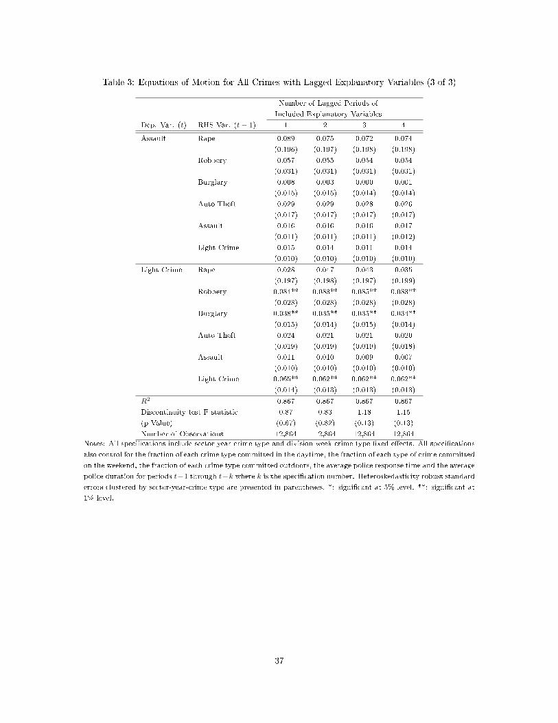
Table 3: Equations of Motion for All Crimes with Lagged Explanatory Variables (3 of 3)

Number of Lagged Periods of

Included Explanatory Variables

Dep. Var. (t) RHS Var. (t− 1) 1 2 3 4

Assault Rape 0.089

(0.196)

0.075

(0.197)

0.072

(0.198)

0.074

(0.198)

Robbery 0.057

(0.031)

0.055

(0.031)

0.054

(0.031)

0.054

(0.031)

Burglary 0.008

(0.015)

0.003

(0.015)

0.000

(0.014)

0.001

(0.014)

Auto Theft 0.029

(0.017)

0.029

(0.017)

0.028

(0.017)

0.026

(0.017)

Assault 0.016

(0.011)

0.016

(0.011)

0.016

(0.011)

0.017

(0.012)

Light Crime 0.015

(0.010)

0.014

(0.010)

0.011

(0.010)

0.014

(0.010)

Light Crime Rape 0.028

(0.197)

0.047

(0.198)

0.043

(0.197)

0.035

(0.199)

Robbery 0.084**

(0.028)

0.083**

(0.028)

0.085**

(0.028)

0.083**

(0.028)

Burglary 0.038**

(0.015)

0.035**

(0.014)

0.035**

(0.015)

0.034**

(0.014)

Auto Theft 0.024

(0.019)

0.021

(0.019)

0.021

(0.019)

0.020

(0.018)

Assault 0.011

(0.010)

0.010

(0.010)

0.009

(0.010)

0.007

(0.010)

Light Crime 0.065**

(0.014)

0.062**

(0.013)

0.062**

(0.013)

0.062**

(0.013)

R2 0.867 0.867 0.867 0.867

Discontinuity test F-statistic

(p-Value)

0.87

(0.67)

0.83

(0.82)

1.18

(0.13)

1.15

(0.13)

Number of Observations 12,864 12,864 12,864 12,864

Notes: All speci�cations include sector-year-crime type and division-week-crime type �xed e�ects. All speci�cations

also control for the fraction of each crime type committed in the daytime, the fraction of each type of crime committed

on the weekend, the fraction of each crime type committed outdoors, the average police response time and the average

police duration for periods t−1 through t−k where k is the speci�cation number. Heteroskedasticity robust standarderrors clustered by sector-year-crime type are presented in parentheses. *: signi�cant at 5% level. **: signi�cant at

1% level.

37

Table 4: Full Estimates, Equations of Motion for All Crimes with up to 4 Lagged ExplanatoryVariables (1 of 3)

Dep. Var. (c) RHS Var βc1 βc

2 βc3 βc

4

Rape Rape 0.011

(0.026)

-0.033

(0.020)

-0.030

(0.022)

-0.035

(0.021)

Robbery -0.005

(0.003)

0.002

(0.003)

0.001

(0.003)

-0.004

(0.003)

Burglary -0.001

(0.002)

0.003

(0.002)

0.001

(0.002)

-0.000

(0.002)

Auto Theft -0.001

(0.002)

-0.002

(0.002)

0.001

(0.002)

-0.000

(0.002)

Assault 0.002

(0.001)

0.002

(0.001)

-0.000

(0.001)

0.002

(0.001)

Light Crime 0.002

(0.001)

-0.001

(0.001)

0.001

(0.001)

-0.000

(0.001)

Robbery Rape 0.079

(0.07)

0.089

(0.075)

0.081

(0.088)

-0.060

(0.079)

Robbery 0.057**

(0.013)

0.023

(0.012)

0.027*

(0.011)

0.009

(0.013)

Burglary 0.007

(0.007)

0.005

(0.006)

0.004

(0.006)

-0.001

(0.006)

Auto Theft -0.004

(0.007)

0.010

(0.007)

-0.006

(0.007)

-0.012

(0.007)

Assault 0.007

(0.004)

0.003

(0.005)

0.004

(0.004)

0.007

(0.005)

Light Crime 0.002

(0.004)

0.003

(0.005)

0.001

(0.004)

-0.008

(0.004)

38

Table 4: Full Estimates, Equations of Motion for All Crimes with up to 4 Lagged ExplanatoryVariables (2 of 3)

Dep. Var. (c) RHS Var βc1 βc

2 βc3 βc

4

Burglary Rape -0.102

(0.143)

0.237

(0.126)

0.251

(0.155)

0.273

(0.149)

Robbery 0.004

(0.024)

0.023

(0.020)

0.021

(0.022)

-0.004

(0.022)

Burglary 0.132**

(0.012)

0.088**

(0.011)

0.034**

(0.012)

0.016

(0.011)

Auto Theft 0.011

(0.013)

0.011

(0.012)

0.009

(0.013)

0.004

(0.013)

Assault -0.008

(0.008)

0.018*

(0.008)

-0.010

(0.008)

-0.008

(0.008)

Light Crime 0.003

(0.008)

0.001

(0.008)

0.018*

(0.008)

0.005

(0.007)

Auto Theft Rape -0.064

(0.130)

-0.030

(0.128)

-0.120

(0.132)

-0.023

(0.128)

Robbery 0.027

(0.016)

-0.001

(0.017)

-0.013

(0.020)

0.009

(0.019)

Burglary 0.004

(0.010)

0.010

(0.010)

0.012

(0.009)

0.003

(0.009)

Auto Theft 0.079**

(0.011)

0.040**

(0.011)

0.032**

(0.011)

0.019

(0.012)

Assault -0.001

(0.006)

0.001

(0.007)

0.005

(0.007)

-0.013*

(0.006)

Light Crime 0.006

(0.008)

0.006

(0.007)

-0.004

(0.006)

0.002

(0.007)

39

Table 4: Full Estimates, Equations of Motion for All Crimes with up to 4 Lagged ExplanatoryVariables (3 of 3)

Dep. Var. (c) RHS Var. βc1 βc

2 βc3 βc

4

Assault Rape 0.074

(0.198)

0.134

(0.194)

-0.019

(0.170)

-0.081

(0.181)

Robbery 0.054

(0.031)

0.001

(0.028)

0.003

(0.024)

0.021

(0.025)

Burglary 0.001

(0.014)

0.024

(0.013)

0.036*

(0.015)

-0.052**

(0.014)

Auto Theft 0.026

(0.017)

-0.003

(0.020)

-0.013

(0.016)

0.027

(0.016)

Assault 0.017

(0.012)

-0.000

(0.012)

0.002

(0.011)

-0.001

(0.013)

Light Crime 0.014

(0.010)

0.008

(0.011)

0.002

(0.011)

0.005

(0.010)

Light Crime Rape 0.035

(0.199)

-0.060

(0.178)

0.082

(0.194)

-0.327

(0.210)

Robbery 0.083**

(0.028)

-0.012

(0.031)

0.016

(0.026)

0.046

(0.028)

Burglary 0.034**

(0.014)

0.014

(0.015)

0.010

(0.015)

-0.010

(0.015)

Auto Theft 0.020

(0.018)

0.040**

(0.015)

-0.007

(0.016)

0.023

(0.019)

Assault 0.007

(0.010)

0.014

(0.011)

0.014

(0.010)

0.008

(0.011)

Light Crime 0.062**

(0.013)

0.025*

(0.011)

0.018

(0.011)

0.013

(0.012)

R2 0.867

Discontinuity test F-statistic

(p-value)

1.15

(0.13)

Number of Observations 12,864

Notes: Each column refers to the lagged coe�cients of our preferred speci�cation, which includes sector-year-crime

type and division-week-crime type �xed e�ects, and also controls for the fraction of each crime type committed

in the daytime, the fraction of each type of crime committed on the weekend, the fraction of each crime type

committed outdoors, the average police response time and the average police duration for periods t − 1 through

t− 4. Heteroskedasticity robust standard errors clustered by sector-year-crime type are presented in parentheses. *:

signi�cant at 5% level. **: signi�cant at 1% level.

40

Table 5: Standard Error Estimates for Equations of Motion in Table 2 at Various Levels of Clus-tering (1 of 3)

Dep. Var. (t) RHS Var. (t− 1) (1) (2) (3) (4) (5) (6)

Rape Rape 0.066**

0.082**

0.048**

0.021*

0.023

0.021*

0.021

0.023

0.021

0.026

0.032

0.027

0.026

0.032

0.027

0.026

0.032

0.027

Robbery 0.003**

0.003**

0.003**

0.002

0.003

0.002

0.003

0.003

0.003

0.003

0.004

0.003

0.003

0.004

0.003

0.003

0.004

0.003

Burglary 0.002

0.002

0.001

0.001*

0.001*

0.001*

0.001

0.001

0.001

0.002

0.002

0.002

0.002

0.002

0.002

0.002

0.002

0.002

Auto Theft 0.002

0.002

0.002

0.002*

0.002

0.001*

0.002

0.002

0.002

0.002

0.002

0.002

0.002

0.002

0.002

0.002

0.002

0.002

Assault 0.001**

0.001**

0.001**

0.001**

0.001**

0.001**

0.001

0.001**

0.001**

0.001

0.001

0.001

0.001

0.001

0.001

0.001

0.001

0.001

Light Crime 0.001**

0.001**

0.001**

0.001**

0.001**

0.001

0.001

0.001

0.001

0.001

0.001

0.001

0.001

0.001

0.001

0.001

0.001

0.001

Robbery Rape 0.093*

0.113

0.069**

0.082

0.06*

0.079

0.073

0.049

0.073

0.074

0.065

0.085

0.074

0.066

0.085

0.074

0.066

0.085

Robbery 0.016**

0.013**

0.010**

0.015**

0.014**

0.010**

0.011**

0.011**

0.010**

0.012**

0.014**

0.013**

0.013**

0.014**

0.013**

0.013**

0.014**

0.013**

Burglary 0.007**

0.008**

0.005**

0.007**

0.008**

0.005**

0.006**

0.006**

0.005*

0.006

0.008

0.006

0.006

0.007

0.006

0.006

0.008

0.006

Auto Theft 0.008**

0.008**

0.005**

0.008**

0.009**

0.006**

0.007**

0.006**

0.006**

0.007

0.007

0.008

0.007

0.007

0.008

0.007

0.007

0.008

Assault 0.005**

0.004**

0.003**

0.005**

0.00**

0.003**

0.005**

0.005**

0.004**

0.004*

0.004*

0.005

0.004*

0.004*

0.005

0.004*

0.004*

0.005

Light Crime 0.013

0.004

0.003**

0.005**

0.004**

0.003**

0.004**

0.005**

0.004**

0.004

0.005

0.005

0.004

0.005

0.005

0.004

0.005

0.005

41

Table 5: Standard Error Estimates for Equations of Motion in Table 2 at Various Levels of Clus-tering (2 of 3)

Dep. Var. (t) RHS Var. (t− 1) (1) (2) (3) (4) (5) (6)

Burglary Rape 0.141

0.165

0.110

0.147

0.150

0.148

0.013

0.134

0.141

0.145

0.146

0.160

0.145

0.146

0.160

0.144

0.146

0.160

Robbery 0.026**

0.024**

0.019**

0.025**

0.024**

0.019**

0.021**

0.025**

0.019**

0.024

0.030

0.023

0.024

0.031

0.023

0.024

0.030

0.023

Burglary 0.019**

0.020

0.010**

0.018**

0.018**

0.010**

0.020**

0.021**

0.011**

0.014**

0.017**

0.013**

0.014**

0.017**

0.013**

0.014**

0.017**

0.013**

Auto Theft 0.015**

0.020**

0.019**

0.015**

0.019**

0.011**

0.014**

0.014*

0.012**

0.013

0.017

0.014

0.013

0.016

0.014

0.013

0.017

0.014

Assault 0.010**

0.011**

0.006**

0.009**

0.009**

0.006**

0.008

0.007*

0.008*

0.007

0.008

0.010

0.007

0.008

0.010

0.007

0.008

0.010

Light Crime 0.010**0.011**

0.007**

0.010**

0.011**

0.007**

0.008**

0.007**

0.007**

0.009

0.009

0.009

0.009

0.009

0.009

0.009

0.009

0.009

Auto Theft Rape 0.126

0.145

0.098

0.125

0.110

0.130

0.115

0.102

0.120

0.128

0.121

0.140

0.128

0.121

0.140

0.128

0.121

0.140

Robbery 0.020**

0.021**

0.016**

0.021**

0.021**

0.016**

0.015**

0.013**

0 .016**

0.016

0.015

0.019

0.016

0.016

0.019

0.016

0.015

0.019

Burglary 0.012**

0.015**

0.007**

0.011**

0.014**

0.007**

0.010**

0.009**

0.008**

0.010

0.013

0.010

0.010

0.013

0.010

0.010

0.013

0.010

Auto Theft 0.015**

0.014**

0.009**

0.015**

0.015**

0.009**

0.015**

0.013**

0.010**

0.012**

0.014**

0.012**

0.012**

0.014**

0.012**

0.012**

0.014**

0.012**

Assault 0.008**

0.009**

0.005**

0.007**

0.010*

0.005**

0.007**

0.008**

0.006**

0.007

0.007

0.008

0.007

0.007

0.008

0.007

0.007

0.008

Light Crime 0.009**

0.010**

0.006**

0.010**

0.010**

0.006**

0.008**

0.009**

0.006**

0.008

0.009

0.008

0.009

0.009

0.008

0.008

0.009

0.008

42

Table 5: Standard Error Estimates for Equations of Motion in Table 2 at Various Levels of Clus-tering (3 of 3)

Dep. Var. (t) RHS Var. (t− 1) (1) (2) (3) (4) (5) (6)

Assault Rape 0.181

0.222

0.147

0.216

0.210

0.208

0.195

0.211

0.189

0.194

0.222

0.209

0.195

0.222

0.210

0.196

0.222

0.210

Robbery 0.035**

0.032**

0.025**

0.033**

0.032**

0.025**

0.031**

0.036**

0.024**

0.030

0.037

0.029

0.031

0.038

0.030

0.031

0.038

0.030

Burglary 0.017**

0.019**

0.012**

0.015**

0.016**

0.012**

0.014**

0.013**

0.012**

0.015

0.011

0.011

0.015

0.011

0.015

0.015

0.011

0.015

Auto Theft 0.020**

0.021**

0.014**

0.021*

0.023

0.014**

0.019**

0.018**

0.014**

0.017

0.018

0.017

0.017

0.018

0.017

0.017

0.018

0.017

Assault 0.016**

0.026**

0.009**

0.014**

0.020**

0.009**

0.016**

0.020**

0.010**

0.012

0.013

0.013

0.011

0.013

0.013

0.011

0.013

0.013

Light Crime 0.012**

0.010**

0.009**

0.013**

0.009**

0.010**

0.012**

0.010**

0.009**

0.010

0.010

0.011

0.010

0.010

0.011

0.010

0.010

0.011

Light Crime Rape 0.172**

0.199**

0.142**

0.201

0.222

0.199

0.181

0.217

0.187

0.195

0.228

0.214

0.196

0.228

0.214

0.197

0.228

0.214

Robbery 0.033**

0.028**

0.023**

0.034**

0.030**

0.023**

0.027**

0.028**

0.024

0.028**

0.032*

0.030**

0.028**

0.032*

0.030**

0.028**

0.032*

0.030**

Burglary 0.018**

0.018**

0.011**

0.018**

0.019**

0.011**

0.014**

0.012**

0.012**

0.015**

0.015**

0.015*

0.015**

0.015**

0.015*

0.015**

0.015**

0.015*

Auto Theft 0.022**

0.022**

0.014**

0.023**

0.023**

0.014**

0.019**

0.020**

0.015**

0.019

0.025

0.018

0.019

0.025

0 .018

0.019

0.025

0.018

Assault 0.011**

0.011**

0.007**

0.011**

0.012**

0.007**

0.011**

0.011**

0.010**

0.010

0.009

0.012

0.010

0.009

0.012

0.010

0.009

0.012

Light Crime 0.017**

0.017**

0.009**

0.017**

0.018**

0.010**

0.014**

0.013**

0.010**

0.014**

0.016**

0.013**

0.014**

0.016**

0.013**

0.014**

0.016**

0.013**

Discontinuity test P-value 0.00**

0.00**

0.00**

0.00**

0.002*

0.001**

0.05*

0.02*

0.09

0.62

0.43

0.88

0.70

0.47

0.91

0.67

0.49

0.91

Notes: Standard error estimates are presented for coe�cients estimated in table 2. The standard errors in bold are

reproduced from table 2 and are clustered at the sector-year-crime type level. The standard errors in normal font are

clustered at the division-year-crime type level. The standard errors in italics are clustered at the division-week-crime

type level. *: coe�cient signi�cant at 5% level. **: coe�cient signi�cant at 1% level.

43

Table 6: Cumulative Reduction in Crimes from Various Crime Elimination Policies

Cumulative Reduction in Crimes from Elimination of:

Crime Rape Robbery Burglary Auto

Theft

Assault Light

Crime

Rape -7.8%* -6.3% 10.9% -4.9% 24.5%* 9.5%

Robbery 2.0% 13.1%** 7.3% -3.4% 11.9%* -0.6%

Burglary 2.6% 2.4% 38.1%** 4.7% -0.5% 7.2%

Auto Theft -0.9% 1.5% 6.1% 20.9%** -1.9% 3.5%

Assault 0.2% 2.1% 1.2% 2.4% 2.2% 3.8%

Light Crime -0.4% 3.7%** 4.8% 4.9%* 4.8%* 13.9%**

Note: Reductions are calculated by hypothetically eliminating one type of crime in the average neighborhood in the

sample for a week, computing the total number of future crimes of each type that is reduced in that neighborhood

and dividing by the average number of weekly crimes of each type in a neighborhood in the sample. For example,

eliminating light crime in the average neighborhood for a week will generate a future reduction in rapes equal to

9.5% of the average number of weekly rapes in a neighborhood in the sample. *: coe�cient signi�cant at 5% level.

**: coe�cient signi�cant at 1% level.

44

Table 7: Estimated Monetary Bene�ts of Unit Crime Reduction

Crime Social Cost of One Unit of

Crime (Miller et al. (1993);

Heaton (2010))

Total Bene�ts from Unit

Crime Reduction ($)

Light Crime Monetary

Equivalents

Rape 239,653 249,357 74.64

Robbery 74,005 86,462 25.88

Burglary 14,406 23,588 7.06

Auto Theft 9,987 12,621 3.78

Assault 22,944 26,429 7.91

Light Crime 1,176 3,341 1

Notes: The social costs of rape, robbery, burglary and auto theft are taken from Heaton (2010). We compute

the social cost of all assaults by taking an average of the social cost of aggravated assault ($95,962) from Heaton

(2010) and the social cost of simple assault ($13,457) from Miller et al. (1993) and weighting by the relative share of

aggravated assaults in our sample (22.83%). We are unable to obtain estimates of the social cost of light crime, so

we assume it to be half of the social cost of larceny as given in Heaton (2010). All monetary amounts are in 2012

dollars.

45

Figure 1: Regression Discontinuity Design: Intuition

- R

6

q

R?(a) Unobservables and Running Variable

- R

6

X

R?(b) Main Explanatory Var. and Running Var.

Note: In these �gures, R is the running variable, X is the main explanatory variable and q contains unobservable

determinants of the outcome variable. The discontinuity threshold is denoted by R?.

46

Figure 2: �Upside-Down� Regression Discontinuity Design: Intuition

- R

6

q

R?(a) Unobservables and Running Variable

- R

6

X

R?(b) Main Explanatory Variable and Running Variable

Note: In these �gures, R is the running variable, X is the main explanatory variable and q contains unobservable

determinants of the outcome variable. The discontinuity threshold is denoted by R?.

47

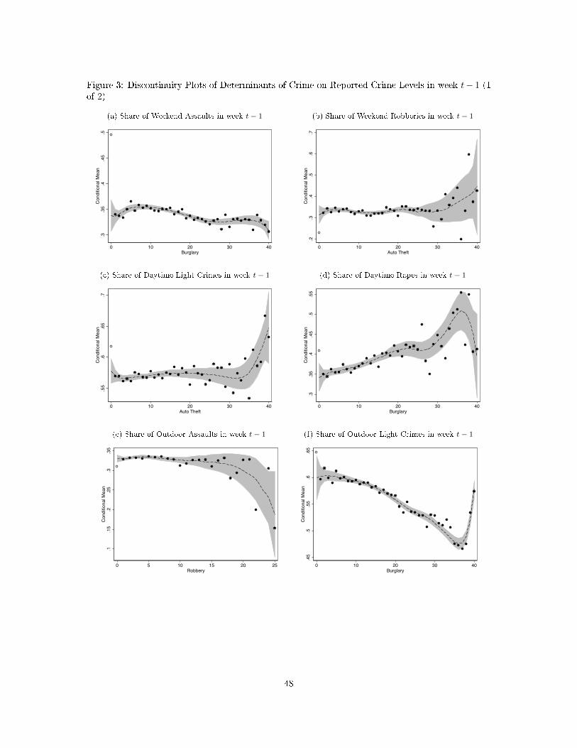
Figure 3: Discontinuity Plots of Determinants of Crime on Reported Crime Levels in week t− 1 (1of 2)

(a) Share of Weekend Assaults in week t− 1

.3.3

5.4

.45

.5C

ondi

tiona

l Mea

n

0 10 20 30 40Burglary

(b) Share of Weekend Robberies in week t− 1

.2.3

.4.5

.6.7

Con

ditio

nal M

ean

0 10 20 30 40Auto Theft

(c) Share of Daytime Light Crimes in week t− 1

.55

.6.6

5.7

Con

ditio

nal M

ean

0 10 20 30 40Auto Theft

(d) Share of Daytime Rapes in week t− 1

.3.3

5.4

.45

.5.5

5C

ondi

tiona

l Mea

n

0 10 20 30 40Burglary

(e) Share of Outdoor Assaults in week t− 1

.1.1

5.2

.25

.3.3

5C

ondi

tiona

l Mea

n

0 5 10 15 20 25Robbery

(f) Share of Outdoor Light Crimes in week t− 1

.45

.5.5

5.6

.65

Con

ditio

nal M

ean

0 10 20 30 40Burglary

48

Figure 3: Discontinuity Plots of Determinants of Crime on Reported Crime Levels in week t− 1 (2of 2)

(g) Police Response to Burglaries in week t (in hours)

1.1

1.2

1.3

1.4

1.5

1.6

Con

ditio

nal M

ean

0 10 20 30 40Auto Theft

(h) Police Response to Light Crime in week t (in hours)

1.2

1.4

1.6

1.8

2C

ondi

tiona

l Mea

n

0 10 20 30 40Auto Theft

(i) Police Response to Light Crimes in week t (in hours)

11.

21.

41.

61.

8C

ondi

tiona

l Mea

n

0 10 20 30 40Burglary

(j) Police Duration at Rape Crime Scenes in week t (inhours)

.51

1.5

2C

ondi

tiona

l Mea

n

0 10 20 30 40Auto Theft

(k) Share of Light Crimes Reported by Businesses inweek t− 1

.06

.08

.1.1

2.1

4.1

6C

ondi

tiona

l Mea

n

0 10 20 30 40Burglary

(l) Share of Auto Thefts Reported by Public Employ-ees in week t− 1

-.002

0.0

02.0

04.0

06.0

08C

ondi

tiona

l Mea

n

0 5 10 15 20 25Robbery

Note: Each point represents the mean of the variable on the y-axis conditional on the number of reports of the

crime on the x-axis. The dashed curve represents a third order local polynomial regression with an Epanechnikov

kernel and bandwidth equals to 5 for both the kernel and the standard error calculation using all points for which

the explanatory variable is positive. The shaded region represents a 95% con�dence region for this regression. The

hollow dot represents the mean of the variable on the y-axis for which there are zero crimes on the x-axis reported.

49

Figure 4: Average Neighborhood Wealth in t− 1 (εt−1)

- εcjt−1

6

xc′

jt−1

E[xc′

jt−1|εcjt−1]

ε?

(a) Past Crime as a Function of Wealth

- xc′

jt−1

6

εcjt−1

E[εcjt−1|xc′

jt−1]

u�E[εcjt−1|xc

′

jt−1 = 0]

ε?

(b) Wealth as a Function of Past Crime

50

Figure 5: Propensity to Misreport Crime in t− 1 (ηt)

- ηcjt

6

xc′

jt−1

E[xc′

jt−1|ηcjt]

η?

(a) Past Crime as a Function of the Propensity to Misreport Crime

- xc′

jt−1

6

ηcjt

E[ηcjt|xc′

jt−1]

u �E[ηcjt|xc

′

jt−1 = 0]

η?

(b) Propensity to Misreport Crime as a Function of Past Crime

51

Figure 6: Unobserved Police Response (Pt) as a Function of Past Crime

- xc′

jt−1

6

P cjt

E[P cjt|xc′

jt−1]

u � E[P cjt|xc′

jt−1 = 0]

52

Figure 7: Cumulative Within-Crime Dynamic Spillovers from Unit Crime Reductions

(a) Speci�cation with 1 Lag

0.0

5.1

.15

.2C

rimes

0 2 4 6 8 10Weeks Elapsed

Rapes RobberyBurglary Auto TheftAssault Light Crime

(b) Speci�cation with 2 Lags

0.1

.2.3

Crim

es

0 2 4 6 8 10Weeks Elapsed

Rapes RobberyBurglary Auto TheftAssault Light Crime

(c) Speci�cation with 3 Lags

-.10

.1.2

.3.4

Crim

es

0 2 4 6 8 10Weeks Elapsed

Rapes RobberyBurglary Auto TheftAssault Light Crime

(d) Speci�cation with 4 Lags

-.10

.1.2

.3.4

Crim

es

0 2 4 6 8 10Weeks Elapsed

Rapes RobberyBurglary Auto TheftAssault Light Crime

53

Figure 8: Cumulative Within- and Across-Crime Dynamic Spillovers From Unit Crime Reductions

(a) Reduction in Rape-.2

0.2

.4.6

.8C

rimes

0 2 4 6 8 10Weeks Elapsed

Rapes RobberyBurglary Auto TheftAssault Light Crime

(b) Reduction in Robbery

0.0

5.1

.15

.2C

rimes

0 2 4 6 8 10Weeks Elapsed

Rapes RobberyBurglary Auto TheftAssault Light Crime

(c) Reduction in Burglary

0.1

.2.3

.4C

rimes

0 2 4 6 8 10Weeks Elapsed

Rapes RobberyBurglary Auto TheftAssault Light Crime

(d) Reduction in Auto Theft

0.0

5.1

.15

.2C

rimes

0 2 4 6 8 10Weeks Elapsed

Rapes RobberyBurglary Auto TheftAssault Light Crime

(e) Reduction in Assault

-.02

0.0

2.0

4.0

6C

rimes

0 2 4 6 8 10Weeks Elapsed

Rapes RobberyBurglary Auto TheftAssault Light Crime

(f) Reduction in Light Crime

0.0

5.1

.15

Crim

es

0 2 4 6 8 10Weeks Elapsed

Rapes RobberyBurglary Auto TheftAssault Light Crime

54

Figure 9: Long Run Cumulative Spillovers From Unit Crime Reductions

-1.2

-1-.8

-.6-.4

-.20

.2.4

.6.8

11.

21.

41.

61.

8

Rap

eR

obbe

ryBu

rgla

ryAu

to T

heft

Assa

ult

Ligh

t Crim

e

Rape

-.20

.2.4

.6

Rap

eR

obbe

ryBu

rgla

ryAu

to T

heft

Assa

ult

Ligh

t Crim

e

Robbery

-.20

.2.4

.6

Rap

eR

obbe

ryBu

rgla

ryAu

to T

heft

Assa

ult

Ligh

t Crim

e

Burglary

-.20

.2.4

.6

Rap

eR

obbe

ryBu

rgla

ryAu

to T

heft

Assa

ult

Ligh

t Crim

e

Auto Theft

-.20

.2.4

.6

Rap

eR

obbe

ryBu

rgla

ryAu

to T

heft

Assa

ult

Ligh

t Crim

e

Assault

-.20

.2.4

.6

Rap

eR

obbe

ryBu

rgla

ryAu

to T

heft

Assa

ult

Ligh

t Crim

e

Light Crime

Cumulative Spillover in:Note: Each of the six panels refers to each type of crime that was reduced by one unit. Vertical bars represent 95% con�dence intervals for long run cumulative

spillovers calculated via the delta method.

55