Do Boys and Girls Use Computers Differently, and Does It ... · Shilpa Aggarwal, Julian Caballero,...

Do Boys and Girls Use Computers Differently, and Does It Contribute to Why Boys do Worse in School than Girls?

Robert W. Fairlie University of California, Santa Cruz

[email protected]

July 2015 Abstract Boys are doing worse in school than are girls, which has been dubbed "the Boy Crisis." An analysis of the latest data on educational outcomes among boys and girls reveals extensive disparities in grades, reading and writing test scores, and other measurable educational outcomes, and these disparities exist across family resources and race. Focusing on disadvantaged schoolchildren, I then examine whether time investments made by boys and girls related to computer use contribute to the gender gap in academic achievement. Data from several sources indicate that boys are less likely to use computers for schoolwork and are more likely to use computers for playing games, but are less likely to use computers for social networking and email than are girls. Using data from a large field experiment randomly providing free personal computers to schoolchildren for home use, I also test whether these differential patterns of computer use displace homework time and ultimately translate into worse educational outcomes among boys. No evidence is found indicating that personal computers crowd out homework time and effort for disadvantaged boys relative to girls. Home computers also do not have negative effects on educational outcomes such as grades, test scores, courses completed, and tardies for disadvantaged boys relative to girls. Keywords: technology, computers, ICT, education, gender, field experiment JEL Codes: C93; I24; J16

I would like to thank Computers for Classrooms, Inc., the ZeroDivide Foundation, and the NET Institute for generous funding for the project. I would also like to thank seminar participants at Stanford University, University of Toronto, Santa Clara University, Wellesley College, the Chicano Latino Research Center at UC Santa Cruz, and Claremont McKenna College for comments and suggestions. I would also like to thank Jennifer Bevers, Bruce Besnard John Bohannon, Linda Coleman, Reg Govan, Rebecka Hagerty, Kathleen Hannah-Chambas, Brian Gault, David Jansen, Cynthia Kampf, Gina Lanphier, Linda Leonard, Kurt Madden, Lee McPeak, Stephen Morris, Joanne Parsley, Richard Pascual, Jeanette Sanchez, Zenae Scott, Tom Sharp, and many others for administering the program in schools. Shilpa Aggarwal, Julian Caballero, David Castaneda, James Chiu, Samantha Grunberg, Brandon Heck, Keith Henwood, Cody Kennedy, Nicole Mendoza, Nick Parker, Miranda Schirmer, Eva Shapiro, Glen Wolf and Heidi Wu are also thanked for research assistance. Finally, special thanks go to Pat Furr for donating many computers for the study and distributing computers to schools.

Do Boys and Girls Use Computers Differently, and Does It Contribute to Why Boys do Worse in School than Girls?

1. Introduction

Boys do worse in school than girls. They obtain lower grades, and are less likely to

graduate from high school and attend college (NCES 2012).1 These gender disparities in

academic performance exist for minority and low-income schoolchildren as well as for more

advantaged schoolchildren. One factor that might contribute to why boys and girls differ in

academic performance is that they make different time investments after school.2 For example,

boys might spend more time playing video games, "playing around" on computers, watching TV,

and using other forms of media than girls. All of these activities might crowd out time spent

doing homework and studying for exams. A recent national time-use diary survey found that

children consume 7 ½ hours of media a day and this level of use is 20 percent higher than it was

only five years ago (Kaiser Family Foundation 2010). The average length of a school day in the

United States is roughly 6 ½ hours (NCES 2012). These time investments made at young ages

between educational and non-educational activities might have long lasting effects on

educational attainment. Surprisingly, very little research has focused on the time investments

made by children and their consequences for educational outcomes.

1 The media has dubbed these disparities as the "Boy Crisis." See "The Boy Crisis. At Every Level of Education, They're Falling Behind. What to Do?" Newsweek (Jan. 30, 2006), "Raising Cain: Boys in Focus," PBS (Jan. 12, 2006), "The Boys Have Fallen Behind," NY Times (March 27, 2010), and "The Boys at the Back," NY Times (February 2, 2013) for example. 2 The reversal of the gender gap in college education with women now earning more college degrees than men has been well documented (see Sundstrom 2004; Goldin, Katz, and Kuziemko 2006 for example), but disparities between boys and girls in academic performance have drawn much less research attention. The underlying causes of these disparities are not well known. Some of the potential explanations examined in recent studies include a disproportionate representation of female teachers in younger grades, girls are more self-disciplined, girls respond more to pre-school interventions, girls are more ready to learn, differential treatment by teachers, and larger positive impacts for girls by Teach for America teachers (Dee 2007; Duckworth and Seligman 2006; Anderson 2008; Cornwell, Mustard and Van Parys 2013; Malamud and Schanzenbach 2007; Antecol, Eren and Ozbeklik 2013).

2

Of particular concern are the potential consequences of computer use among boys and

girls. Computer use is one of the largest types of media use among children (Kaiser Family

Foundation 2010), and thus extensive use of computers after school for video games, social

networking and other entertainment activities might crowd out homework and study time among

schoolchildren. There is evidence in the previous literature of computer use crowding out

schoolwork and negative effects on academic performance. For example, Malumed and Pop-

Eleches (2011) find evidence of heavy game use of computers and negative effects of computers

on reading, homework and grades, and Fuchs and Woessmann (2004) find a negative

relationship between home computers and math and reading test scores, possibly due to the

distracting effects of children "playing computer games."3 If boys have higher levels of access to

home computers, use computers more for playing games, or use computers less for schoolwork

than girls, computers may partly contribute to why boys do worse in school. A better

understanding of these potential effects is especially important for low-income and minority

schoolchildren because of the policy focus on expanding access to technology to reduce the

digital divide.4

In this paper, I first examine the latest national data on academic performance among

girls and boys focusing on disadvantaged schoolchildren. I then explore three hypotheses

3 Concerns over the negative effects of home computers have gained a fair amount of attention recently in the press. See, for example, "Computers at Home: Educational Hope vs. Teenage Reality," NY Times, July 10, 2010 and "Wasting Time Is New Divide in Digital Era," NY Times, May 29, 2012. Extensive use of social networking sites, such as Facebook, is one particular concern (e.g., see Karpinski 2009; Pasek and Hargittai 2009). These concerns are similar to those over television (e.g., see Zavodny 2006). 4 The U.S. federal government spends more than $2 billion per year on the E-rate program, which provides discounts to schools and libraries for the costs of telecommunications services and equipment (Puma, et al. 2000, Universal Services Administration Company 2013). England provided free computers to nearly 300,000 low-income families with children at a total cost of £194 million through the Home Access Programme. Additional policies include tax breaks, special loans and Individual Development Accounts (IDA) for educational purchases of computers, community technology centers, and laptop checkout programs for students (Servon 2002, Lazarus 2006, and Gordo 2008).

3

regarding computer use and these differences. First, I examine whether girls and boys have

differential access rates to personal computers at home. Using microdata from the Computer and

Internet Supplement to the Current Population Survey (CPS), I examine whether computer

access rates vary across boy-only, girl-only and boy-girl families, and whether there are gender

differences for low-income and minority schoolchildren. Second, I explore whether

disadvantaged boys and girls use computers differently. Are boys more likely to use computers

for video games and other non-educational activities, and are they less likely to use computers

for schoolwork? Although a few previous studies examine gender differences in computer and

Internet use among adults, very little is known about gender differences in the use of computers

among children.5 Using data from three sources, I conduct the first detailed examination of

computer and Internet use among boys and girls. Computer use for game playing, social

networking, schoolwork and other activities is examined.

Third, I explore whether boy-girl differences in computer use crowd out homework time

and effort differently, and contribute to gender disparities in educational outcomes among

disadvantaged schoolchildren. To test this hypothesis I estimate the effects of home computers

on homework time and effort, grades, standardized test scores, and several additional educational

outcomes for girls and boys. Given similar access rates, if home computers have a larger

negative impact on educational outcomes for boys than for girls then differential computer use at

home widens the achievement gap. If instead, home computers have a similar effect for boys and

girls then differential computer use does not contribute to the achievement gap. To remove

5 Men and women are found to have very similar levels of access to computers and the Internet, but differ in intensity of use and activities, and possibly benefits (see Ono and Zavodny 2003; Hargittai 2007; Mossberger 2008; NTIA 2011; Figlio, et al. 2012 for example). Differences in access and use, however, are substantially larger by race and income (see Hoffman and Novak 1998; Mossberger, Tolbert, and Stansbury 2003; Mossberger, Tolbert, and Gilbert 2006; Ono and Zavodny 2007; Fairlie 2004; Goldfarb and Prince 2008 for example).

4

concerns about selection bias resulting from which families decide to purchase computers I use

data from the largest-ever randomized control experiment providing free personal computers to

U.S. schoolchildren for home use.6 Half of over one thousand schoolchildren grades 6-10

attending 15 different schools were randomly selected to receive computers to use at home.

Previous findings for all schoolchildren participating in the field experiment indicate that the

randomly selected group of students receiving free computers experienced no improvement in

educational outcomes relative to the control group that did not receive free computers (Fairlie

and Robinson 2013). Fairlie and Robinson (2013), however, does not explore whether boys and

girls use computers differently and whether these differences contribute to the gender gap in

academic performance among disadvantaged schoolchildren.

Briefly previewing the results, I find that girls outperform boys not only in grades, test

scores in reading and writing, and high school graduation rates, but also in numerous other

educational outcomes. The results show a remarkably consistent underperformance of boys

relative to girls in school, which holds across race and family resources. Using microdata from

the CPS computer supplement I find that boys and girls have very similar rates of access to home

computers overall and by race and income even though disparities across these groups are large.

Boys and girls use computers differently, however, with boys using computers more for video

games and girls using computers more for schoolwork, email and social networking, which does

not differ substantially by race or income. Estimates from the random experiment, however, do

not provide evidence that computers crowd out homework time and effort for disadvantaged

6 If computers were exogenously assigned to children the question could be explored by simply comparing the girl-boy gap in educational outcomes among existing computer owners to the girl-boy gap in educational outcomes among existing non-computer owners. But, parents make decisions about computer purchases partly based on concerns about the non-educational uses of computers by children and partly based on the perceived educational benefits of computers to children (which might differ between boys and girls) raising concerns about selection bias.

5

boys relative to girls, or that home computers have negative effects on grades, test scores, and

other educational outcomes for boys relative to girls. Although parents, schools, and

policymakers may have other concerns about how boys and girls use computers, these patterns

do not appear to contribute to why disadvantaged boys do worse in school than girls.

The remainder of the paper is organized as follows. In Section 2, I describe the data

sources used to examine gender differences in computer access and use. I also describe the

experiment used to test for gender differences in the impacts of computers on educational

outcomes. Section 3 presents estimates of gender differences in academic performance. Section 4

presents estimates of gender differences in computer access and use. Section 5 presents the

experimental results for the impacts of home computers on homework time and effort and

educational outcomes for boys and girls. Section 5 concludes.

2. Data and Methods

Data on Computer Use

Data from three national sources are used to examine whether boys and girls use

computers differently. I use data from the Current Population Survey Computer and Internet Use

Supplements conducted by the U.S. Bureau of Labor Statistics and Census Bureau, a time use

diary study of the use of technology by children conducted by the Kaiser Family Foundation, and

surveys of teenagers conducted as part of the Pew Internet and American Life Project. The

combination of data from these national sources provides the first comprehensive examination of

gender differences in computer use among children.

The Internet and Computer Use Supplement to the Current Population Survey (CPS),

conducted by the U.S. Census Bureau and the Bureau of Labor Statistics, is representative of the

6

entire U.S. population and interviews approximately 50,000 households and 130,000 individuals.

The Internet and Computer Use Supplement to the CPS is the primary source of information on

technology use collected by the federal government and has been conducted over the past three

decades at irregular intervals. The information gathered differs in each survey. Estimates from

the 2003 supplement include the latest information on computer use activities among children.

The estimates reported later in Table 4 are from these CPS data. The 2011 Supplement is the

latest available data, but does not allow one to examine activities of computer use among

children (only adult householders). Because of the lack of published results from the survey, I

use microdata from the 2011 CPS Supplement to examine overall access and use rates among

boys and girls ages 5-17 (N=23,594). The microdata also allow for a more detailed examination

of home computer access rates among girls and boys by child and family characteristics such as

the gender composition of the household, race, income, and age.

The Kaiser Family Foundation surveyed 2,002 children ages 8-18 across the country in

2008 and 2009 on their use of media including detailed information on computer use (Kaiser

Family Foundation 2010). Similar surveys were conducted in 1999 and 2004 by the Kaiser

Family Foundation. Information on computer use activities is also reported from national surveys

conducted as part of the Pew Internet and American Life Project (see Pew Internet Project 2008a,

2008b). Surveys on numerous topics related to computer, Internet and media use are conducted

regularly by the Pew Research Center. The Pew Internet Project (2008a, 2008b) studies include

nationally-representative samples of 1,102 children ages 12-17 in 2007 and 2008 and 700

children ages 12-17 in 2007, respectively. To our knowledge, these three sources of data

represent all of the nationally representative sources of data providing detailed information on

computer use among children.

7

Randomized Control Experiment

To explore the effects of personal computers on crowding out homework time and

educational outcomes among disadvantaged boys and girls and whether these effects differ by

gender I use data from a field experiment that provides free personal computers to schoolchildren

for home use. The randomized control experiment involved 1,123 students in grades 6-10

attending 15 schools across California (see Fairlie and Robinson 2013 for more details). It

represents the first field experiment involving the provision of free computers to schoolchildren

for home use ever conducted, and the largest experiment involving the provision of free home

computers to U.S. students at any level. The randomized control experiment removes concerns

about selection bias resulting from which families decide to purchase computers. All of the

students participating in the study did not have computers at baseline. Half were randomly

selected to receive free computers, while the other half served as the control group. Outcomes

were tracked for all participating students over an academic year.

The sample for this study includes 1,123 students enrolled in grades 6-10 in 15 different

middle and high schools in 5 school districts in California. The project took place over two

years: two schools participated in 2008-9, twelve schools participated in 2009-10, and one school

participated in both years. The 15 schools in the study span the Central Valley of California

geographically. Overall, these schools are similar in size (749 students compared to 781

students), student to teacher ratio (20.4 to 22.6), and female to male student ratio (1.02 to 1.05)

as California schools as a whole (U.S. Department of Education 2011). Schools in the

experiment, however, are poorer (81% free or reduced price lunch compared with 57%) and have

a higher percentage of minority students (82% to 73%) than the California average reflecting the

8

requirement of not having a home computer for eligibility in the experiment. Participating

students also have lower average test scores than the California average (3.2 compared with 3.6

in English-Language Arts and 3.1 compared with 3.3 in Math), but the differences are not large

(California Department of Education 2010).

To identify children who did not already have home computers, we conducted an in-class

survey at the beginning of the school year with all of the students in the 15 participating schools.

The survey, which took only a few minutes to complete, asked basic questions about home

computer ownership and usage. To encourage honest responses, it was not announced to students

that the survey would be used to determine eligibility for a free home computer (even most

teachers did not know the purpose of the survey). In total, 7,337 students completed in-class

surveys, with 24 percent reporting not having a computer at home. This rate of home computer

ownership is roughly comparable to the national average: – estimates from the 2010 Current

Population Survey indicate that 27% of children aged 10-17 do not have a computer with

Internet access at home (U.S. Department of Education 2011).

Any student who reported not having a home computer on an in-class survey was eligible

for the study.7 All eligible students were given an informational packet, baseline survey, and

consent form to complete at home. To participate, children had to have their parents sign the

consent form (which, in addition to participating in the study, released future grade, test score

and administrative data) and return the completed survey to the school. Of the 1,636 students

eligible for the study, we received 1,123 responses with valid consent forms and completed

7 Because eligibility for the study is based on not having a computer at home, our estimates capture the impact of computers on the educational outcomes of schoolchildren whose parents do not buy them on their own and do not necessarily capture the impact of computers for existing computer owners. Schoolchildren without home computers, however, are the population of interest in considering policies to expand access.

9

questionnaires (68.6%). We randomized treatment at the individual level, stratified by school. In

total, of the 1,123 participants, 559 were randomly assigned to the treatment group. For boys,

there were 555 participants with 280 assigned to the treatment group, and for girls there were

568 participants with 279 assigned to the treatment group.

The computers provided through the experiment were purchased from or donated by

Computers for Classrooms, Inc., a Microsoft-certified computer refurbisher located in Chico,

California. The computers were refurbished Pentium machines with 17" monitors, modems,

ethernet cards, CD drives, flash drives, Microsoft Windows, and Microsoft Office (Word, Excel,

PowerPoint, Outlook). The computer came with a 1-year warranty on hardware and software

during which Computers for Classrooms offered to replace any computer not functioning

properly. In total, the retail value of the machines was approximately $400-500 a unit. Since the

focus of the project was to estimate the impacts of home computers on educational outcomes and

not to evaluate a more intensive technology policy intervention, no training or assistance was

provided with the computers. We did not provide Internet service as part of the experiment and

found that about half of the students receiving computers subscribed to service.

The computers were handed out by the schools to eligible students in the late fall of the

school year. Almost all of the students sampled for computers received them: we received

reports of only 11 children who did not pick up their computers, and 7 of these had dropped out

of their school by that time. As expected, we found that some of the control group students

purchased home computers by the end of the school year. From a follow-up survey conducted at

the end of the school year, we found that 27 percent of girls and 25 percent of boys in the control

group purchased computers, and in most cases these computers were purchased later in the

school year (thus having less potential impacts on measured outcomes). After the distribution,

10

neither the research team nor Computers for Classrooms had any contact with students during the

school year. In addition, many of the outcomes were collected at least 6 months after the

computers were given out (for example, end-of-year standardized test scores and fourth quarter

grades). Thus, it is very unlikely that student behavior would have changed for any reason other

than the computers themselves (for instance, via Hawthorne effects).

Data from the experiment were collected from four main sources. First, we administered

a detailed baseline survey which was required to participate in the project (as that was where

consent was obtained). The survey includes detailed information on student and household

characteristics. Second, we administered a follow-up survey at the end of the school year, which

included detailed questions about computer ownership, homework time, and homework effort

allowing for a comparison of first-stage and homework crowd-out effects. The response rates for

the follow-up survey were high: 78.2 percent for boys and 76.6 percent for girls.8 Third, each

school provided us with detailed administrative data on educational outcomes for all students

covering the entire academic year. These administrative data include grades in all courses taken

and disciplinary information. Finally, schools provided us with standardized test scores from the

California Standardized Testing and Reporting (STAR) program. A major advantage of the

administrative data on test scores as well as grades and other outcomes is that they are measured

without any measurement error, and attrition is virtually non-existent. The collection of these

datasets provides an extensive amount of information on computer ownership and educational

outcomes.

Randomization and Implementation Checks

8 The response rates are 76.7 percent for the control group and 79.6 percent for the treatment group for boys, and 75.4 percent for the control group and 77.8 percent for the treatment group for girls.

11

Appendix Table 1 reports summary statistics for the treatment and control groups and

provides a balance check. Balance checks are reported for the total sample, the girl sample, and

the boy sample. For each sample, means for the treatment and control groups and the p-value for

a t-test of equality are reported. Overall, there is very little difference between the treatment and

control groups in all three samples. The only variable with a difference that is statistically

significant is that treatment children are less likely to live with their mother in the boy sample

(although the difference of 0.06 is small relative to the base of 0.93). It is likely that this one

difference is caused by random chance given the large number of comparisons being made –

nevertheless, all of these covariates are controlled for in the regressions that follow.

As a check of the experimental implementation, I also examine whether there is a large

relative increase in reported computer ownership and whether the effect is similar for boys and

girls. Information on computer ownership is obtained from the follow-up survey conducted at the

end of the school year. For girls, I find that 82% of the treatment group and 27% of the control

group report having a computer at follow-up. For boys, the overall levels are similar and the

treatment-control difference is identical, with 80% of the treatment group and 25% of the control

group reporting having a computer at follow-up. While these treatment-control differences of 55

percentage points are very large, if anything they are understated because only a very small

fraction of the 559 students in the treatment group did not receive one (as noted above, we had

reports of only 11 students who did not pick up their computer). In fact, I find that one quarter of

the boy and girl treatment groups report positive hours of computer use at home even though

they report in a previous question that they do not have a computer at home and are supposed to

skip the question. In addition, any measurement error in computer ownership would understate

differences in reported ownership.

12

The follow-up survey also asked children a battery of questions about how much they use

computers for five different types of activities at home, school, and other locations. With the

resulting 15 different questions of types of use, the self-reported hours responses are noisy with

many missing values and some inconsistencies in reporting. Appendix Table 2 reports the

average value of responses to these questions. Overall, computer use increased for both boys and

girls. This includes separate use for schoolwork, email, games, and social networking.

Unfortunately, the estimates are not precise enough to identify girl-boy differences in use. With

so many different categories to report hours of use there is likely to be a fair amount of

measurement error in these estimates, and thus I do not place too much weight on them.

These results are suggestive of three important findings regarding first-stage effects.

First, the experiment had a large effect for both boys and girls on increasing computer

ownership. Second, the increase in computer ownership was similar for girls and boys. Third, the

experiment also increased computer use for both boys and girls for numerous activities.

3. Girl-Boy Differences in Academic Performance

I first examine girl-boy differences in academic performance. Figure 1 reports average

grades for boys and girls from the High School Transcript Study which is part of the National

Assessment of Educational Progress (NAEP) conducted by the National Center for Educational

Statistics (NCES). The latest available data is for 2009 and grades are available overall and in

several different subjects. The estimates clearly indicate that girls obtain better grades than boys.

They have higher overall grades than boys and obtain better grades in every core subject matter.

The disparities are large. Even in math and science, girls obtain grades that are nearly 0.2 points

13

higher, and in English grades are over 0.3 points higher (which is equivalent to a + or – modifier

on a letter grade).

Gender differences are large among disadvantaged schoolchildren. Table 1 reports

average grades by parental education and race (which are the categories available in the NAEP

grade data). Boys from families with low parental education or from underrepresented minority

groups have lower grades in all subjects than girls from similar families. In fact, the grade

underperformance of boys relative to girls is large across all parental education groups and all

racial groups.

Figure 2 reports test score data for boys and girls collected as part of the 2011 NAEP.

Overall girls score better, on average, than boys on reading and writing assessment tests,

similarly on math assessment tests, but slightly lower on science assessment tests. Table 2

reports test scores by school lunch eligibility and race (which are the categories available in the

NAEP test score data). The girl-boy patterns in test scores across subjects (i.e. girls score higher

in reading and writing, similarly in math, and slightly lower in science than boys) hold for low-

income and minority schoolchildren.

Using the NAEP data on test scores, I also examine girl and boy distributions of test

scores. Figure 3 reports inverse cumulative distribution functions for each of the test scores

reported in Figure 2 for both boys and girls. The distributional estimates are limited by NAEP

reporting to showing the 10th, 25th, 50th, 75th, and 90th percentiles, but these percentiles

characterize the full distribution reasonably well. Because I report inverse CDFs, the vertical

difference at each of the reported points in the distribution is the equivalent to a quantile

treatment effect (QTE) estimate. In addition to girls having higher average test scores in reading

and writing, girls have higher test scores throughout the distribution. At each reported percentile

14

girls have higher scores than boys. For math test scores, girls and boys have roughly similar

scores throughout the distribution with some slight differences at the reported tails. For science

test scores, the distribution for boys is slightly higher at all points.

In addition to performing better on grades, and reading and writing test scores, girls

outperform boys along numerous other measures of educational outcomes. Girl-boy disparities in

many of these measures are not as well-known as those for grades, high school graduation rates,

and college attendance. Appendix Table 3 provides evidence of consistent and sizeable gender

disparities in several educational outcomes starting with outcomes relevant to school entry and

ending with high school graduation.

The evidence clearly indicates that boys are doing worse in school than girls.

Schoolchildren from disadvantaged families are no exception, with minority and low-income

boys having lower grades in all subjects and test scores in some subjects than girls. Although

some of these differences in academic performance have received attention recently, we know

relatively little about differences in computer access, use, and a broader set of after-school time

investments made by boys and girls.

4. Girl-Boy Differences in Computer Access and Use

Microdata from the computer supplement to the 2011 CPS is first used to explore

whether girls and boys have similar levels of access to computers at home. Table 3 reports home

computer access rates for girls and boys. Overall, boys and girls have identical rates of access to

computers at home. The lack of differences by gender is not simply due to boys and girls living

in the same households. Even in households with only boys or only girls access rates are

identical. Among low-income families and disadvantaged minorities, boys and girls also have

15

similar access rates to home computers. This finding of lack of girl/boy differences in computer

access differs substantially from the large differences found by race or income (see Hoffman and

Novak 1998; Mossberger, Tolbert, and Stansbury 2003; Ono and Zavodny 2003b; Fairlie 2004;

Goldfarb and Prince 2008 for example). Ruling out gender differences in access to home

computers is important because it focuses the analysis on differential use of computers between

boys and girls, which is examined next.

Data from three national sources are used to examine whether disadvantaged boys and

girls use computers differently. I use microdata from the 2003 CPS Computer and Internet Use

Supplement, microdata from surveys of teenagers conducted as part of the Pew Internet and

American Life Project, and a time use diary study of the use of technology by children conducted

by the Kaiser Family Foundation. Table 4 reports gender differences in use. Focusing on how

boys and girls use computers reveals some interesting differences. I find consistent evidence of

four main patterns across the datasets. First, I find that girls are more likely than boys to use

computers for schoolwork (although these differences are not large). Second, boys spend more

time playing video games on computers than do girls. Third, I find some evidence that girls use

computers more for social networking, email, and other communication activities. Finally, these

patterns are similar for low-income and high-income children.

These results provide some evidence that boys and girls use computers differently, but it

is not clear whether these differences lead to differential effects of home computers on crowding

out homework and educational outcomes, and thus contribute to the gender achievement gap.

Unfortunately, this question is not an easy one to answer empirically. One possibility is to

conduct an experiment in which computers are randomly taken away from schoolchildren who

already own them and examine their subsequent academic performance. Another approach,

16

which is much more feasible, is to conduct a random experiment providing computers to

schoolchildren who do not already own them and examine their subsequent academic

performance.9 I take this approach next.

5. Girl-Boy Differences in Impacts of Computers on Crowding Out Homework and

Educational Outcomes

In this section, I examine whether computers crowd out homework time and effort

differently for boys and girls, and whether computers have differential impacts on the

educational outcomes of boys and girls. Recent research focusing on all children finds mixed

results on the impacts of home computers on educational outcomes, but none of these studies

focus on differential impacts by gender and their implications for the gender gap in academic

achievement.10 To examine whether home computers have differential educational impacts for

boys and girls using the experimental data, I can simply calculate treatment-control differences

in mean values of each measure for the boy and girl samples separately. To improve precision

and confirm the robustness of the results to randomization, however, I estimate several

regressions for homework time and educational outcomes. The regression equation is

straightforward in the context of the random experiment:

(1) Yi = α + βGTiGi + βBTiBi + θGi + δXi + εi,

9 The alternative approaches also have different implications for external validity. An experiment taking the former approach focuses on a more advantaged group whereas as an experiment taking the latter approach focuses on a less advantaged group. The two groups may use computers differently. 10 See Schmitt and Wadsworth (2004); Fairlie (2005); Fuchs and Woessmann (2004); Fiorini (2010); Beltran, et al. (2010); Malamud and Pop-Eleches (2010); Beuermann et al. (2012); Fairlie and Robinson (2013); Vigdor, et al. (2014); Falck, et al. 2015 for example, and see Bulman and Fairlie (2015) for a recent review of the literature.

17

where Yi is the outcome for student i (e.g. grade), Ti is an indicator variable for being in the

treatment group, Gi is an indicator for girls, Bi is an indicator for boys, Xi includes the baseline

characteristics such as demographic and family characteristics reported in Appendix Table 1, and

εi is an error term. The separate effects of becoming eligible for a free computer or the "intent-to-

treat" estimate of the giveaway program are captured by βG for girls and βB for boys,

respectively. The differential impact of home computers on educational outcomes between girls

and boys is equal to βG-βB. All specifications are estimated using OLS and robust standard errors

are reported with adjustments for multiple observations per student (i.e. clustered by student)

when needed for grades.11 The standard error for βG-βB is estimated from the re-specified

regression:

(2) Yi = α + βBTi + (βG-βB)TiGi + θGi + δXi + εi.

Marginal effects estimates are similar from probit and logit models, and are thus not reported.

I first examine whether obtaining a computer crowds out homework time and effort for

boys relative to girls using information collected from our follow-up survey. Table 5 reports

estimates of home computer effects on self-reported measures of time spent doing homework,

turning assignments in on time, and how much time is spent on the last essay or report. I report

estimates of treatment effects separately for boys and girls and the difference between the two

(which is estimated in a separate regression to obtain the standard error). Home computers do not

crowd out homework time for boys relative to girls. The point estimate on the girl-boy treatment

11 For all regressions for each educational outcome, I include controls for the sampling strata (school*year) in addition to the controls listed in Appendix Table 1. To avoid dropping observations, for each control variable, I create a dummy equal to 1 if the variable is missing for a student and code the original variable as a 0 (so that the coefficients are identified from those with non-missing values). Estimates are similar when I instead exclude these observations (there are only a few missing values).

18

is actually negative, although small and statistically insignificant. Obtaining a personal computer

also has no negative effect on whether boys report turning in homework on time relative to girls.

Finally, the computers did not appear to result in boys spending less time working on essays than

girls.

Overall, there is no evidence indicating that computers crowd out homework time and

effort for boys relative to girls. Another interesting finding is that in absolute terms I also do not

find evidence that computers crowd out homework time and effort among boys (or girls).

Turning to educational outcomes, I examine whether home computers have a negative

effect on grades, test scores, total courses completed and tardies obtained from administrative

data from each of the schools. Table 6 reports estimates of the separate effects of home

computers on grades for boys and girls and the difference between the two.12 Panel A reports

estimates of treatment effects on overall grades and grades in academic subjects (i.e. math,

English, social studies, science) for boys and girls and the difference between the two. For the

grade regressions, I pool the quarter 3 and 4 grades together. I find similar results when I

estimate separate regressions for quarter 3 and quarter 4. I also include controls for quarter 1

grades, the subject and quarter in the regressions. Grades are coded as A-4, B-3, C-2, D-1, F-0.

+/- modifiers are set equal to 0.33 points. In all cases, I find no evidence of a positive or negative

effect of computers on grades for boys or girls.13 Similarly, home computers do not have a

differential effect on grades for boys and girls.

12 I focus on grades first because of their importance in determining high school graduation and college admissions (Betts and Morrell 2009). 13 LATE (or IV) estimates would be about twice as large (since the difference in computer usage is 55 percentage points). I do not report these estimates, however, because I cannot technically scale up the coefficients with the IV estimator because of differential timing of purchasing computers over the school year by the control group (two thirds of the control group with a home computer at follow-up obtained this computer after the fall). The finding that 80-82 percent of the treatment group reports having a computer at the end of the school year also creates difficulty in scaling up the ITT estimates because I

19

In Columns 3-4, I supplement the overall grade estimate by focusing on the effects of

home computers on the pass/fail part of the grade distribution. In all of the schools, a grade of D-

or higher is considering passing and provides credit towards moving to the next grade level and

graduation. Again, I find no evidence of a differential effect of home computers between boys

and girls. Expanding the distribution even further, I focus on the effects of home computers on

the probability of obtaining a grade of B or higher (columns 5-6) and a grade of A or higher

(columns 7-8). In both cases, I find no evidence of a differential effect of home computers for

boys and girls. Estimates from quantile regressions for the full post-treatment achievement

distribution confirm these findings (not reported). I do not find evidence of a clear pattern of

differential treatment effects across the distribution.

I also examine whether treatment effects differ by subject. The finding for overall grades

holds when examining courses separately by subject. Girls perform better in all subjects than

boys, but home computers have no differential effect, either negative or positive, on grades for

any subject. The lack of a negative relative effect for boys suggests that home computers are not

contributing to why boys have lower grades in all subjects than girls. The finding holds for both

average grades and along the pass/fail margin.

Related to this issue, I examine whether there are differential treatment effects across the

pre-treatment grade distribution. There might be negative relative treatment effects for boys for

some parts of the distribution that cannot be identified focusing on the average treatment effect. I

estimate the following regression:

(2) ∗ ∗ ∗ ∗

know that essentially all treatment students picked up their computers and that many of the treatment group reporting not having a computer at follow-up indeed had a computer at home (based on subsequent conversations with the students by principals). For these reasons I focus on the ITT estimates.

20

In the regression, is an indicator for whether individual i is in the pth percentile of the pre-

treatment GPA distribution. Percentiles are calculated within each school and are restricted to 20

different percentile categories. is an indicator for the control group, and is an indicator for

the treatment group. Thus, and are estimates of the relationship between pre- and post-

treatment performance in the control and treatment groups, respectively, and the difference,

provides an estimate of the treatment effect at the pth percentile. is a minimal set of

controls, including only subject and quarter indicators (so that the coefficients represent the

unconditional relationship between pre- and post-performance for the treatment and control

groups). and are reported in Figure 4a for girls and Figure 4b for boys. Standard errors

are clustered at the individual level, and the 95% confidence interval of the difference between

the treatment and control groups is plotted.

The estimates displayed in the figures indicate that treatment effects are indistinguishable

from zero at almost all points of the pre-treatment grade distribution for both girls and boys.

Thus, I do not find evidence of differential effects of home computers for boys and girls across

the distribution.

I also estimate the impacts of home computers performance on the California

Standardized Testing and Reporting (STAR) Program tests. As part of the STAR Program, all

California students are required to take standardized tests for English-Language Arts and math

each spring. For regressions in which test scores are the dependent variable, I focus on two key

measures. First, I report estimates for a standardized test score based on raw values. These test

scores are normalized to have mean 0 and standard deviation 1. I also report estimates for an

indicator of proficiency. This variable is coded as 1 if the student receives a 4 or 5 (out of 5) on

the test, and 0 otherwise. Proficiency and advanced scores meet state standards and are important

21

for schools to satisfy Adequate Yearly Progress (AYP) as part of the No Child Left Behind Act.

Table 7 reports estimates of the effects of home computers on test scores in

English/Language Arts and mathematics. For both test scores, and whether I use a standardized

test score or an indicator for meeting proficiency levels, I do not find evidence that home

computers have a differential effect for boys and girls.

In addition to not finding a differential effect between girls and boys at the proficiency

level I also do not find effects throughout the distribution. Plots of inverse cumulative

distribution functions (CDFs) for both boys and girls reveal substantial overlap between the

treatment and control groups for both test scores.14 The lack of treatment effects across the

distribution implies that there are no differential effects between boys and girls. Similarly,

Figures 5 and 6 examine the effects of home computers on STAR scores by prior achievement

levels. Again, there is no discernible effect at almost any point in the pre-treatment STAR

distribution. The finding holds for both English/Language Arts and math test scores. These

figures suggest minimal effects of computers across the pre-treatment ability distribution and

rule out the possibility that the null estimates of average treatment effects are due to offsetting

positive and negative treatment effects at different parts of the pre-treatment achievement

distribution. Most importantly, the lack of treatment effects for both boys and girls implies no

differential effects throughout the distribution.

I also examine the effects of home computers on total courses completed and number of

tardies. Estimates are reported in Columns 5-7 of Table 7. I find no evidence of a differential

effect of home computers on total courses completed in the 3rd and 4th quarters of the academic

14 I examined inverse CDFs because the STAR scores are lumped into only 5 bins and thus I cannot estimate quantile treatment effects.

22

year. Estimates from the experiment also do not indicate that differential effects of home

computers explain boy-girl differences in being tardy for school.

For all of the educational outcomes examined there is no evidence of a negative relative

effect for boys suggesting that home computers and their use cannot explain why boys generally

do worse in school than girls.

6. Conclusions

The results from this study provide the first evidence in the literature on whether

disadvantaged boys and girls use computers differently, whether home computers crowd out

homework time differently for boys and girls, and whether home computers have differential

effects on educational outcomes among boys and girls. Although estimates from the CPS

indicate that girls and boys have similar rates of access to home computers, evidence from

several sources of data indicate that boys use computers differently than girls. Boys use

computers less for schoolwork and more for playing games, but less for communication such as

through social networking, email and instant messaging, than girls. Using data from a large field

experiment that randomly provides free personal computers to schoolchildren for home use, I test

the hypothesis that these gender differences in computer use partly explain why boys generally

do worse than girls in school. I do not find evidence that computers crowd out homework time

and effort more for boys than for girls. Examining impacts on grades, test scores and additional

educational outcomes, the evidence does not indicate negative effects of home computers for

boys relative to girls. I do not find differential effects at notable points in the distribution such as

pass rates and meeting proficiency standards, or throughout the distribution of post-treatment

outcomes.

23

Disadvantaged boys and girls differ in how they use computers, but these differences do

not appear to lead to different levels of crowding out of homework and study time, and do not

ultimately lead to different grades, test scores and other educational outcomes. Thus, gender

differences in time investments in how personal computers are used at home do not appear to

contribute to the achievement gap between disadvantaged boys and girls. This finding has

implications for the general view that girls are more "self-disciplined" than are boys. Both girls

and boys are found here to use computers for non-educational activities, but for both boys and

girls these activities do not appear to crowd out homework time and negatively affect

performance in school.

For the broader picture of the girl-boy achievement gap, identifying, or ruling out,

potential explanations for why boys are doing worse in school than girls is extremely important.

Some policy recommendations include increasing the number of male teachers at young grades,

all-boy classrooms, more hands-on activities, and more frequent or longer recesses. Recent

trends in educational outcomes do not show relative improvement for boys, and differences

between boys and girls are quite large. The girl-boy difference in grades of 0.2 grade points is

only slightly smaller than the white-Latino difference of 0.25 grade points and half the white-

black difference of 0.4 grade points. The racial achievement gap, however, has attracted

considerably more attention in the literature and policy arena (e.g. Jencks and Phillips 1998).

Further research on the causes of gender differences in educational outcomes especially among

disadvantaged and low-income children is clearly needed.

24

References Anderson, Michael. 2008. "Multiple Inference and Gender Differences in the Effects of Early Intervention: A Reevaluation of the Abecedarian, Perry Preschool, and Early Training Projects." Journal of the American Statistical Association, 103(484): 1481-1495. Antecol, Heather, Ozkan Eren, and Serkan Ozbeklik. 2013. The effect of Teach for America on the distribution of student achievement in primary school: Evidence from a randomized experiment, Economics of Education Review, 37: 113–125.

Beltran, Daniel O., Kuntal K. Das, and Robert W. Fairlie. 2010. "Home Computers and Educational Outcomes: Evidence from the NLSY97 and CPS," Economic Inquiry 48(3): 771-792. Betts, Julian and Darlene Morell. 1999. "The Determinants of Undergraduate Grade Point Average: The Relative Importance of Family Background, High School Resources, and Peer Group Effects." Journal of Human Resources, Vol. 34, No. 2: 268-93. Beuermann, Diether W., Julián P. Cristia, Yyannu Cruz-Aguayo, Santiago Cueto, and Ofer Malamud. 2012. "Home Computers and Child Outcomes: Short-Term Impacts from a Randomized Experiment in Peru," Inter-American Development Bank Working Paper No. IDB-WP-382.

Bulman, George, and Robert W. Fairlie. 2015. "Technology and Education: Computers, Software, and the Internet " Handbook of the Economics of Education, Volume 5, eds. Rick Hanushek, Steve Machin, and Ludger Woessmann, North-Holland.

California Department of Education. 2010. 2010 STAR Test Results: California STAR Program, http://star.cde.ca.gov/star2010/ Cornwell, Christopher M., David B. Mustard, and Jessica Van Parys. 2013. "Non-cognitive Skills and the Gender Disparities in Test Scores and Teacher Assessments: Evidence from Primary School." Journal of Human Resources, 48(1): 236-264. Dee, Thomas S. 2007. "Teachers and the Gender Gaps in Student Achievement," Journal of Human Resources, XLII(3): 528-554. Duckworth, Angela Lee, and Martin E. P. Seligman. 2006. "Self-Discipline Gives Girls the Edge: Gender in Self-Discipline, Grades, and Achievement Test Scores," Journal of Educational Psychology, 98(1): 198–208. Fairlie, Robert W. 2004. "Race and the Digital Divide," Contributions to Economic Analysis & Policy, The Berkeley Electronic Journals 3(1), Article 15: 1-38. Fairlie, Robert W. 2005. "The Effects of Home Computers on School Enrollment," Economics of Education Review 24(5): 533-547.

25

Fairlie, Robert W., and Jonathan Robinson. 2013. "Experimental Evidence on the Effects of Home Computers on Academic Achievement among Schoolchildren." American Economic Journal: Applied Economics, 5(3): 211-40. Falck, Oliver, Constantin Mang, and Ludger Woessmann. 2015. “Virtually No Effect? Different Types of Computer Use and the Effect of Classroom Computers on Student Achievement,” CESifo Working Paper No. 5266.

Figlio, David, Mark Rush, and Lu Yin. 2013. "Is It Live or Is It Internet? Experimental Estimates of the Effects of Online Instruction on Student Learning." Journal of Labor Economics 31(4): 763-784. Fiorini, M. 2010. “The Effect of Home Computer Use on Children’s Cognitive and Non-Cognitive Skills,” Economics of Education Review 29: 55-72. Fuchs, Thomas, and Ludger Woessmann. 2004. "Computers and Student Learning: Bivariate and Multivariate Evidence on the Availability and Use of Computers at Home and at School." CESifo Working Paper No. 1321. Goldfarb, Avi, and Jeffrey Prince. 2008. "Internet Adoption and Usage Patterns are Different: Implications for the Digital Divide." Information Economics and Policy 20(1), 2-15. Goldin, Claudia, Lawrence Katz, and Ilyana Kuziemko (2006). "The Homecoming of American College Women: The Reversal of the College Gender Gap." Journal of Economic Perspectives. Gordo, Blanca. 2008. Disconnected: A Community and Technology Needs Assessment of the Southeast Los Angeles Region. Center for Latino Policy Research, UC Berkeley Report.

Hargittai, Eszter. 2007. "Whose Space? Differences among Users and Non-Users of Social Network Sites," Journal of Computer-Mediated Communication 13(1): 276–297. Hoffman, Donna L. and Thomas P. Novak. 1998. "Bridging the Racial Divide on the Internet." Science 17 April: 390-391. Jencks, Christopher, and Meredith Phillips. 1998. The Black-White Test Score Gap, Washington, DC: Brookings Institution Press.

Kaiser Family Foundation. 2010. Generation M2: Media in the Lives of 8- to 18-Year Olds. Kaiser Family Foundation Study. Karpinski, A.C. 2009. “A description of Facebook use and academic performance among undergraduate and graduate students,” paper presented at the Annual Meeting of the American Educational Research Association, San Diego, Calif.

26

Lazarus, Wendy. 2006. California Competes: Deploying Technology to Help California Youth Compete in a 21st-Century World: A Three-Point Digital Opportunity Action Plan, Children’s Partnership Report.

Malamud, Ofer, and Cristian Pop-Eleches. 2011. "Home Computer Use and the Development of Human Capital," Quarterly Journal of Economics 126: 987-1027. Malamud, Ofer and Diane Schanzenbach (2007). "The Disparity between Boys' Performance and Teacher Evaluations during Elementary School." University of Chicago working paper. Mossberger, Karen. 2008. “Toward Digital Citizenship: Addressing Inequality in the Information Age,” in Handbook of Internet Politics, Andrew Chadwick and Philip Howard, eds. London: Routledge. Mossberger, K., C. Tolbert, and M. Stansbury. 2003. Virtual Inequality: Beyond the Digital Divide. Georgetown University Press, Washington, DC. Mossberger, K., C. Tolbert, and M. Gilbert. 2006. "Race, Place, and Information Technology," Urban Affairs Review, 41(5): 583-620.

National Telecommunications and Information Administration. 2011. Digital Nation: Expanding Internet Usage, Washington, D.C.: U.S. Department of Commerce, National Telecommunications and Information Administration. National Center for Educational Statistics. 2011. Digest of Educational Statistics 2011, Washington, D.C.: U.S. Department of Education, National Center for Educational Statistics. National Center for Educational Statistics. 2012. Youth Indicators 2011: America's Youth: Transitions to Adulthood, Washington, D.C.: U.S. Department of Education, National Center for Educational Statistics. Ono, Hiroshi, and Madeline Zavodny. 2003. “Gender and the Internet,” Social Science Quarterly 84(1): 111–121.

Ono, Hiroshi, and Madeline Zavodny. 2007. “Digital Inequality: A Five Country Comparison Using Microdata,” Social Science Research, 36 (September 2007): 1135-1155.

Pasek, Josh, and Eszter Hargittai. 2009. "Facebook and academic performance: Reconciling a media sensation with data," First Monday, Volume 14, Number 5 - 4.

Pew Internet Project. 2008. Teens, Video Games, and Civics, Washington, D.C.: Pew Internet & American Life Project.

Pew Internet Project. 2008. Writing, Technology and Teens, Washington, D.C.: Pew Internet & American Life Project.

27

Puma, Michael J., Duncan D. Chaplin, and Andreas D. Pape. 2000. E-Rate and the Digital Divide: A Preliminary Analysis from the Integrated Studies of Educational Technology. Urban Institute.

Servon, Lisa. 2002. Bridging the Digital Divide: Community, Technology and Policy (Blackwell).

Servon, Lisa J., and Marla K. Nelson. 2001. Community Technology Centers: Narrowing the Digital Divide in Low-Income, Urban Communities, Journal of Urban Affairs, 23(3-4): 279–290.

Schmitt, John, and Jonathan Wadsworth. 2006. "Is There an Impact of Household Computer Ownership on Children's Educational Attainment in Britain?" Economics of Education Review, 25: 659-673.

Sundstrom, William A. 2004. " The College Gender Gap in Comparative Perspective, 1950-2000," Santa Clara University, Department of Economics Working Paper.

U.S. Department of Education. 2011. “School Locator,” National Center for Educational Statistics, http://nces.ed.gov/ccd/schoolsearch/

Universal Services Administration Company. 2013. Annual Report http://www.usac.org/about/tools/publications/annual-reports/default.aspx.

Vigdor, Jacob L., Helen F. Ladd, and Erika Martinez. 2014. “Scaling the Digital Divide: Home Computer Technology and Student Achievement,” Economic Inquiry. 52(3): 1103–1119.

Zavodny, Madeline. 2006. “Does Watching Television Rot Your Mind? Estimates of the Effect on Test Scores,” Economics of Education Review 25: 565-573.

28

2.0

2.2

2.4

2.6

2.8

3.0

3.2

3.4

3.6

Overall Mathematics Science English Social Studies

Figure 1: Grade Point Average by Gender and SubjectHigh School Transcript Study, 2009

Girls

Boys

29

100

150

200

250

300

Math (4th Grade) Math (8th Grade) Science (8th Grade) Reading (4th Grade) Reading (8th Grade) Writing (8th Grade) Writing (12th Grade)

Figure 2: Average Test Scores by Gender and SubjectNational Assessment of Educational Progress, 2011

Girls

Boys

30

Figure 3.A: Inverse CDF for Test Scores (Reading and Writing)National Assessment of Educational Progress, 2011

165.0

185.0

205.0

225.0

245.0

265.0

0 0.5 1

Reading (4th Grade)

Boys

Girls

210.0

230.0

250.0

270.0

290.0

310.0

0 0.5 1

Reading (8th Grade)

Boys

Girls

90.0

110.0

130.0

150.0

170.0

190.0

210.0

0 0.5 1

Writing (8th Grade)

Boys

Girls

90.0

110.0

130.0

150.0

170.0

190.0

0 0.5 1

Writing (12th Grade)

Boys

Girls

31

Figure 3.B: Inverse CDF for Test Scores (Math and Science)National Assessment of Educational Progress, 2011

200.0

210.0

220.0

230.0

240.0

250.0

260.0

270.0

280.0

0 0.5 1

Math (4th Grade)

Boys

Girls

230

250

270

290

310

330

0% 50% 100%

Math (8th Grade)

Boys

Girls

100.0

120.0

140.0

160.0

180.0

200.0

0 0.5 1

Science (8th Grade)

Boys

Girls

32

Figure4.Post‐TreatmentGradesbyPre‐TreatmentGPAPercentile

PanelA.Girls

PanelB.Boys

Notes:Thegraphshowsestimatedcoefficientsfromaregressionofpost‐treatment(quarters3and4)gradesoninteractionsbetweentreatmentandpre‐treatmentGPApercentile(inquarter1,beforethecomputersweregivenout).Theverticallineisa95%confidenceintervalforthedifferencebetweenthetreatmentandcontrolgroups,ateachpercentile.Seetextformoredetails.

0.5

11

.52

2.5

33

.54

Po

st-t

rea

tme

nt g

rad

e

.05 .15 .25 .35 .45 .55 .65 .75 .85 .95Percentile in pre-treatment grade distribution

Control Treatment95% CI of difference

Post-Treatment Grades by Pre-Treatment GPA Percentile

0.5

11

.52

2.5

33

.54

Po

st-t

rea

tme

nt g

rad

e

.05 .15 .25 .35 .45 .55 .65 .75 .85 .95Percentile in pre-treatment grade distribution


Post-Treatment Grades by Pre-Treatment GPA Percentile

33

Notes:ThegraphshowsestimatedcoefficientsfromaregressionofendlineSTARscoresoninteractionsbetweentreatmentandpre‐treatmentSTARscores.Theverticallineisa95%confidenceintervalforthedifferencebetweenthetreatmentandcontrolgroups,ateachpercentile.Seetextformoredetails.

PanelA.Girls

PanelB.Boys

Figure5.Post‐TreatmentEnglish/LanguageArtsSTARscoresbyPre‐TreatmentStarPercentiles

0.5

11

.52

2.5

33

.54

4.5

5E

ndl

ine

ST

AR

sco

re

.05 .15 .25 .35 .45 .55 .65 .75 .85 .95Percentile in pre-treatment STAR score distribution


Endline STAR Score by Pre-Treatment STAR Score Percentile0

.51

1.5

22

.53

3.5

44

.55

En

dlin

e S

TA

R s

core



Endline STAR Score by Pre-Treatment STAR Score Percentile

34

Figure6.Post‐TreatmentMathSTARscoresbyPre‐TreatmentStarPercentiles

PanelA.Girls

PanelB.Boys

Notes:ThegraphshowsestimatedcoefficientsfromaregressionofendlineSTARscoresoninteractionsbetweentreatmentandpre‐treatmentSTARscores.Theverticallineisa95%confidenceintervalforthedifferencebetweenthetreatmentandcontrolgroups,ateachpercentile.Seetextformoredetails.

0.5

11

.52

2.5

33

.54

4.5

5E

ndl

ine

ST

AR

sco

re



Endline STAR Score by Pre-Treatment STAR Score Percentile0

.51

1.5

22

.53

3.5

44

.55

En

dlin

e S

TA

R s

core



Endline STAR Score by Pre-Treatment STAR Score Percentile

35

Table1.GradePointAveragebyGender,ParentalEducationandRace

Girls BoysGirl‐BoyDifference

Grade Point Average (Overall)

All Students 3.10 2.90 0.20

Parental Education: High School Dropout 2.88 2.75 0.13

Parental Education: Graduated High School 2.98 2.77 0.21

Parental Education: Graduated College 3.27 3.04 0.23

Race: White 3.20 2.98 0.22

Race: Black 2.79 2.57 0.22

Race: Hispanic 2.91 2.75 0.16

Race: Asian 3.37 3.15 0.22

Grade Point Average (Mathematics)





Race: White 2.84 2.63 0.21

Race: Black 2.41 2.23 0.18


Race: Asian 3.09 2.94 0.15

Grade Point Average (Science)

Average 2.78 2.61 0.17




Race: White 2.89 2.70 0.19

Race: Black 2.47 2.24 0.23


Race: Asian 3.10 2.93 0.17

Grade Point Average (English)





Race: White 3.11 2.77 0.34

Race: Black 2.71 2.37 0.34


Race: Asian 3.30 2.97 0.33

Grade Point Average (Social Studies)



Parental Education: Graduated High School 2.86 2.62 0.24Parental Education: Graduated College 3.20 2.96 0.24Race: White 3.10 2.88 0.22Race: Black 2.68 2.43 0.25Race: Hispanic 2.78 2.60 0.18

Race: Asian 3.28 3.05 0.23

Source:HighSchoolTranscriptStudy,2009.

36

Table2.AverageTestScoresbyGender,SchoolLunchEligibilityandRace


Average Test Score (Math 4th Grade)

All Students 240 241 ‐1

Eligible for National School Lunch Program 229 229 0

Not Eligible for National School Lunch Program 251 253 ‐2

Race: White 248 251 ‐3

Race: Black 225 225 0

Race: Hispanic 231 232 ‐1

Race: Asian 260 260 0

Average Test Score (Math 8th Grade)






Race: Hispanic 272 272 0

Race: Asian 310 311 ‐1

Average Test Score (Science 8th Grade)


Eligible for National School Lunch Program 135 139 ‐4



Race: Black 127 130 ‐3

Race: Hispanic 136 140 ‐4

Race: Asian 161 164 ‐3

Average Test Score (Reading 4th Grade)

All Students 225 219 6


Not Eligible for National School Lunch Program 239 233 6

Race: White 235 229 6




Average Test Score (Reading 8th Grade)








Average Test Score (Writing 8th Grade)








Average Test Score (Writing 12th Grade)








Source:NationalAssessmentofEducationalProgress,2011.

37

Table3.AccesstoPersonalComputersatHomebyBoysandGirls


Total 84% 84% 0%Girlonlyhousehold 85%Boyonlyhousehold 85%Girlandboyhousehold 83% 83% 0%Ages5‐9 81% 82% 0%Ages10‐14 85% 84% 1%Ages15‐17 86% 87% 0%Familyincome<$20,000 62% 60% 2%Familyincome$20,000‐39,999 75% 75% ‐1%Familyincome$40,000‐74,999 91% 92% ‐1%

Familyincome$75,000‐99,999 97% 96% 1%Familyincome$100,000ormore 98% 97% 1%White,non‐Hispanic 91% 91% 1%Hispanic 70% 71% ‐1%Black 75% 75% 0%Asian 93% 96% ‐3%Source:CurrentPopulationSurvey,ComputerandInternetSupplement2011Microdata.

Percentwithaccesstoahomecomputer

38

Table4.ComputerUsebyGenderandFamilyIncome


CurrentPopulationSurvey2003PercentofInternetusersusingforplayinggames 61% 68% ‐7%Low‐incomechildren 59% 65% ‐6%High‐incomechildren 63% 69% ‐6%PercentofInternetusersusingforemailandmessaging 64% 57% 7%Low‐incomechildren 52% 49% 3%High‐incomechildren 69% 60% 9%PercentofInternetusersusingforschoolassignments 79% 77% 2%Low‐incomechildren 75% 73% 2%High‐incomechildren 80% 78% 2%PercentusingInternetanywhere 61% 58% 3%Low‐incomechildren 49% 46% 3%High‐incomechildren 70% 69% 1%

PewInternetStudy(2007‐08)Percentplayingvideogamesdaily 22% 39% ‐17%Low‐incomechildren 23% 40% ‐17%High‐incomechildren 20% 37% ‐17%Percentsendingemailonadailybasis 20% 12% 8%Low‐incomechildren 20% 11% 9%High‐incomechildren 17% 10% 7%PercentusingInterneteverforschoolresearch 96% 92% 4%Low‐incomechildren 89% 88% 1%High‐incomechildren 97% 92% 5%

KaiserFoundationTimeUseDiary2009Minutesofcomputeruseforplayinggames 8 25 ‐17Minutesofcomputeruseforvideosandotherentertainmen 19 23 ‐4Minutesofcomputeruseforsocialnetworking 25 19 6Minutesofcomputeruseforemailandinstantmessaging 18 16 2Minutesofcomputeruseforotheractivities 12 14 ‐2Minutesofcomputeruseforschoolwork 19 13 6Totalminutesperdayofcomputeruse 101 110 ‐9

Sources:KaiserFamilyFoundation(2010);MicrodatafromthePewInternetProjects(2008a,2008b);CurrentPopulationSurvey,ComputerandInternetSupplement2003microdata.

39

Table5.ExperimentalEstimatesofComputerCrowd‐OutImpactsonHomeworkTimeandEffort(1) (2) (3) (4) (5)

Always Usually Sometimes

Girltreatment ‐0.38 ‐0.01 ‐0.02 0.03 ‐0.22(0.38) (0.05) (0.05) (0.04) (1.15)

Boytreatment 0.20 ‐0.07 0.07 0.00 0.16(0.39) (0.05) (0.05) (0.04) (1.17)

Girl‐boytreatmentdiff. ‐0.58 0.06 ‐0.10 0.04 ‐0.38(0.56) (0.07) (0.07) (0.05) (1.66)

Observations 825 853 853 853 805Girlcontrolmean 2.79 0.48 0.37 0.15 4.02Boycontrolmean 2.49 0.46 0.38 0.17 4.77

Howmuchtimedidyouspendonlast

essay?

Howoftendoyouturninhomeworkontime?

Howmanyhoursperweekdoyouspendonhomework?

Notes:Dataisfromfollow‐upsurveycompletedbystudentsatendofschoolyear.Regressionsincludecontrolsforsamplingstrata(school*year)andvariableslistedinAppendixTable1.***,**,*indicatessignificanceat1,5and10%.

40

Table6.ExperimentalEstimatesofHomeComputerImpactsonGrades(1) (2) (3) (4) (5) (6) (7) (8)

AllsubjectsAcademicSubjects




PanelA.ClassGradesGirltreatment 0.00 0.04 0.01 0.02 ‐0.01 0.00 ‐0.02 0.00

(0.05) (0.06) (0.01) (0.01) (0.02) (0.02) (0.02) (0.02)Boytreatment ‐0.03 0.00 ‐0.01 ‐0.02 ‐0.01 0.01 0.00 0.01

(0.05) (0.06) (0.01) (0.02) (0.02) (0.02) (0.02) (0.02)Girl‐boytreatmentdiff. 0.03 0.04 0.02 0.03 0.00 ‐0.02 ‐0.01 ‐0.01

(0.08) (0.09) (0.02) (0.02) (0.03) (0.03) (0.03) (0.03)Observations 11514 7820 11514 7820 11514 7820 11514 7820Numberofstudents 1036 1035 1036 1035 1036 1035 1036 1035Girlcontrolmean 2.58 2.40 0.90 0.89 0.59 0.53 0.33 0.27Boycontrolmean 2.37 2.10 0.86 0.83 0.52 0.43 0.28 0.20

MathEnglish/Reading

SocialStudies

Science MathEnglish/Reading

SocialStudies

Science

PanelB.ClassGradesbySubjectGirltreatment 0.03 ‐0.06 0.12 0.09 0.02 ‐0.01 0.05 0.01

(0.09) (0.08) (0.09) (0.08) (0.03) (0.02) (0.02)** (0.02)Boytreatment 0.01 ‐0.14 0.07 0.08 0.00 ‐0.03 ‐0.01 ‐0.03

(0.09) (0.09) (0.10) (0.09) (0.03) (0.03) (0.03) (0.03)Girl‐boytreatmentdiff. 0.02 0.08 0.05 0.01 0.02 0.02 0.06 0.04

(0.13) (0.12) (0.13) (0.12) (0.04) (0.03) (0.04) (0.03)Observations 1886 2121 1784 1895 1886 2121 1784 1895Numberofstudents 969 903 921 960 969 903 921 960Girlcontrolmean 2.05 2.65 2.45 2.42 0.83 0.92 0.88 0.89Boycontrolmean 1.93 2.28 2.10 2.05 0.81 0.85 0.82 0.82

Notes:Regressionsincludecontrolsforsamplingstrata(school*year),variableslistedinAppendixTable1,andpreviousgrades.***,**,*indicatessignificanceat1,5and10%.

GradesIndicatorforpassing

classIndicatorforBorHigherGrade

IndicatorforAorHigherGrade

Grade Indicatorforpassingclass

41

Table7.ExperimentalEstimatesofHomeComputerImpactsonTestScoresandOtherEducationalOutcomes(1) (2) (3) (4) (5) (6) (7)

English/Lang.Arts

MathEnglish/Lang.Arts

MathIn3rdquarter

In4thquarter

NumberofTardies

Girltreatment ‐0.10 0.02 ‐0.02 ‐0.03 ‐0.01 0.04 0.18(0.06) (0.07) (0.03) (0.04) (0.13) (0.14) (1.31)

Boytreatment 0.00 ‐0.13 0.02 0.00 0.09 ‐0.10 ‐0.72(0.07) (0.07)* (0.03) (0.04) (0.14) (0.14) (1.34)

Girl‐boytreatmentdiff. ‐0.10 0.15 ‐0.04 ‐0.03 ‐0.10 0.15 0.90(0.09) (0.10) (0.05) (0.05) (0.19) (0.20) (1.89)

Observations 961 914 961 914 1123 1123 1104Girlcontrolmean 0.13 ‐0.04 0.33 0.29 5.42 5.54 9.65Boycontrolmean ‐0.13 0.04 0.25 0.31 5.30 5.43 13.49

StandardizedScore ProficiencyIndicator TotalCreditsEarned

Notes:Regressionsincludecontrolsforsamplingstrata(school*year),variableslistedinAppendixTable1,andprevioustestscores.***,**,*indicatessignificanceat1,5and10%.

42

AppendixTable1.IndividualLevelSummaryStatisticsandBalanceCheck

Age 12.91 12.90 0.91 12.92 12.85 0.37 12.90 12.96 0.46(0.87) (0.84) (0.91) (0.78) (0.83) (0.89)

Female 0.51 0.50 0.66 1 1 0 0(0.50) (0.50)

Ethnicity=AfricanAmerican 0.13 0.14 0.86 0.14 0.13 0.66 0.13 0.15 0.50(0.34) (0.34) (0.35) (0.34) (0.33) (0.35)

Ethnicity=Latino 0.56 0.55 0.76 0.55 0.57 0.66 0.57 0.54 0.38(0.50) (0.50) (0.50) (0.50) (0.50) (0.50)

Ethnicity=Asian 0.12 0.14 0.42 0.12 0.14 0.49 0.12 0.13 0.66(0.33) (0.34) (0.33) (0.35) (0.33) (0.34)

Ethnicity=White1 0.16 0.14 0.56 0.16 0.14 0.61 0.15 0.15 0.76(0.36) (0.35) (0.37) (0.35) (0.36) (0.35)

Immigrant 0.21 0.18 0.15 0.21 0.18 0.40 0.21 0.17 0.23(0.41) (0.38) (0.41) (0.39) (0.41) (0.38)

PrimarylanguageisEnglish 0.43 0.43 0.97 0.43 0.43 0.98 0.43 0.43 0.97(0.50) (0.50) (0.50) (0.50) (0.50) (0.50)

Parent'seducation2 12.81 12.76 0.64 12.71 12.77 0.67 12.94 12.75 0.22(1.44) (1.49) (1.48) (1.50) (1.39) (1.48)

Numberofpeoplelivinginhousehold 4.98 5.02 0.79 5.03 5.13 0.62 4.93 4.92 0.95(2.43) (2.55) (2.34) (2.47) (2.53) (2.63)

Liveswithmother 0.92 0.89 0.12 0.90 0.91 0.77 0.93 0.87 0.014**(0.28) (0.32) (0.30) (0.29) (0.25) (0.34)

Liveswithfather 0.58 0.58 0.90 0.53 0.56 0.48 0.64 0.60 0.33(0.49) (0.49) (0.50) (0.50) (0.48) (0.49)

Doesyourmotherhavejob?4 0.47 0.46 0.68 0.47 0.44 0.55 0.47 0.48 0.98(0.50) (0.50) (0.50) (0.50) (0.50) (0.50)

Doesyourfatherhaveajob? 0.73 0.70 0.36 0.70 0.65 0.41 0.77 0.74 0.66(0.44) (0.46) (0.46) (0.48) (0.43) (0.44)

Fullsamplesize 564 559 289 279 275 280

TreatmentEqualityofmeansp‐value

Notes:InColumns1,2,4,5,7and8,meansreportedwithstandarderrorsinparentheses.Column3,6and9reportthep‐valueforthet‐testfortheequalityofmeans.***,**,*indicatessignificanceat1,5and10%.1 Omittedethnicitycategoryis"notreported."2 Thisisthehighesteducationlevelofeitherparent(whichisthemeasuremostschoolsinoursamplecollected).3 Thevariablesformother'sandfather'sjobisreportedonlyforhouseholdsinwhichthegivenparentlivesinthehousehold.

Total Girls Boys

Control TreatmentEqualityofmeansp‐value

Control TreatmentEqualityofmeansp‐value

Control

43

AppendixTable2.First‐StageEffectsonReportedHoursofComputerUsebyLocationandTypeofActivity(1) (2) (3) (4) (5)

Schoolwork EmailGames,Videos,Music,Ent.

SocialNetworking

Other

PanelA.TotalGirlcontrolgroup 2.10 0.27 0.58 0.44 0.54Girltreatmentgroup 2.84 0.59 1.27 1.07 0.77Treatment‐control 0.74 0.31 0.69 0.63 0.23

(0.36)** (0.17)* (0.29)** (0.24)** ‐0.14Boycontrolgroup 1.67 0.20 0.99 0.68 0.58Boytreatmentgroup 2.57 0.74 1.74 1.12 0.77Treatment‐control 0.90 0.54 0.75 0.44 0.19

(0.35)** (0.16)*** (0.28)*** (0.24)* ‐0.14Girl‐BoyTreatment‐Control ‐0.16 ‐0.23 ‐0.06 0.19 0.04

(0.51) (0.23) (0.40) (0.34) (0.20)Observations 665 665 665 665 665

PanelB.AtHomeGirlcontrolgroup 0.22 0.05 0.12 0.14 0.13Girltreatmentgroup 1.03 0.29 0.65 0.49 0.35Treatment‐control 0.81 0.24 0.54 0.35 0.22

(0.16)*** (0.09)*** (0.15)*** (0.12)*** (0.07)***Boycontrolgroup 0.21 0.08 0.23 0.12 0.10Boytreatmentgroup 0.98 0.33 0.81 0.62 0.34Treatment‐control 0.77 0.25 0.59 0.49 0.24

(0.16)*** (0.09)*** (0.15)*** (0.12)*** (0.07)***Girl‐BoyTreatment‐Control 0.04 ‐0.01 ‐0.05 ‐0.14 ‐0.02

(0.23) (0.13) (0.21) (0.17) (0.10)Observations 789 789 789 789 789

PanelC.AtSchoolGirlcontrolgroup 1.11 0.06 0.16 0.05 0.23Girltreatmentgroup 0.97 0.05 0.12 0.03 0.17Treatment‐control ‐0.15 ‐0.01 ‐0.04 ‐0.01 ‐0.06

‐0.16 ‐0.03 ‐0.11 ‐0.02 ‐0.07Boycontrolgroup 0.91 0.07 0.30 0.08 0.27Boytreatmentgroup 1.11 0.05 0.39 0.04 0.13Treatment‐control 0.20 ‐0.02 0.09 ‐0.04 ‐0.15

‐0.16 ‐0.03 ‐0.11 (0.02)* (0.07)**Girl‐BoyTreatment‐Control ‐0.35 0.01 ‐0.13 0.02 0.08

(0.22) (0.04) (0.16) (0.03) (0.10)Observations 771 771 771 771 771

PanelD.AtOtherLocationsGirlcontrolgroup 0.76 0.15 0.29 0.23 0.24Girltreatmentgroup 0.59 0.20 0.36 0.44 0.22Treatment‐control ‐0.17 0.04 0.06 0.21 ‐0.02

‐0.19 ‐0.11 ‐0.10 ‐0.16 ‐0.08Boycontrolgroup 0.53 0.09 0.48 0.47 0.23Boytreatmentgroup 0.43 0.36 0.48 0.46 0.30Treatment‐control ‐0.10 0.27 0.01 ‐0.01 0.07

‐0.19 (0.11)** ‐0.10 ‐0.16 ‐0.08Girl‐BoyTreatment‐Control ‐0.06 ‐0.23 0.06 0.22 ‐0.09

(0.27) (0.16) (0.14) (0.23) (0.11)Observations 771 771 771 771 771

HoursofComputerUsePerWeek

Notes:Dataarefromfollow‐upsurveycompletedbystudentsatendofschoolyear.***,**,*indicatessignificanceat1,5and10%.

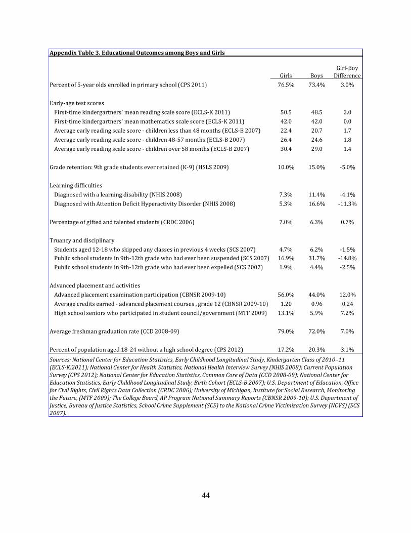
44

AppendixTable3.EducationalOutcomesamongBoysandGirls


Percentof5‐yearoldsenrolledinprimaryschool(CPS2011) 76.5% 73.4% 3.0%

Early‐agetestscores

First‐timekindergartners'meanreadingscalescore(ECLS‐K2011) 50.5 48.5 2.0

First‐timekindergartners'meanmathematicsscalescore(ECLS‐K2011) 42.0 42.0 0.0

Averageearlyreadingscalescore‐childrenlessthan48months(ECLS‐B2007) 22.4 20.7 1.7

Averageearlyreadingscalescore‐children48‐57months(ECLS‐B2007) 26.4 24.6 1.8

Averageearlyreadingscalescore‐childrenover58months(ECLS‐B2007) 30.4 29.0 1.4

Graderetention:9thgradestudentseverretained(K‐9)(HSLS2009) 10.0% 15.0% ‐5.0%

Learningdifficulties

Diagnosedwithalearningdisability(NHIS2008) 7.3% 11.4% ‐4.1%

DiagnosedwithAttentionDeficitHyperactivityDisorder(NHIS2008) 5.3% 16.6% ‐11.3%

Percentageofgiftedandtalentedstudents(CRDC2006) 7.0% 6.3% 0.7%

Truancyanddisciplinary

Studentsaged12‐18whoskippedanyclassesinprevious4weeks(SCS2007) 4.7% 6.2% ‐1.5%Publicschoolstudentsin9th‐12thgradewhohadeverbeensuspended(SCS2007) 16.9% 31.7% ‐14.8%

Publicschoolstudentsin9th‐12thgradewhohadeverbeenexpelled(SCS2007) 1.9% 4.4% ‐2.5%

Advancedplacementandactivities

Advancedplacementexaminationparticipation(CBNSR2009‐10) 56.0% 44.0% 12.0%

Averagecreditsearned‐advancedplacementcourses,grade12(CBNSR2009‐10) 1.20 0.96 0.24

Highschoolseniorswhoparticipatedinstudentcouncil/government(MTF2009) 13.1% 5.9% 7.2%

Averagefreshmangraduationrate(CCD2008‐09) 79.0% 72.0% 7.0%

Percentofpopulationaged18‐24withoutahighschooldegree(CPS2012) 17.2% 20.3% 3.1%

Sources:NationalCenterforEducationStatistics,EarlyChildhoodLongitudinalStudy,KindergartenClassof2010–11(ECLS‐K:2011);NationalCenterforHealthStatistics,NationalHealthInterviewSurvey(NHIS2008);CurrentPopulationSurvey(CPS2012);NationalCenterforEducationStatistics,CommonCoreofData(CCD2008‐09);NationalCenterforEducationStatistics,EarlyChildhoodLongitudinalStudy,BirthCohort(ECLS‐B2007);U.S.DepartmentofEducation,OfficeforCivilRights,CivilRightsDataCollection(CRDC2006);UniversityofMichigan,InstituteforSocialResearch,MonitoringtheFuture,(MTF2009);TheCollegeBoard,APProgramNationalSummaryReports(CBNSR2009‐10);U.S.DepartmentofJustice,BureauofJusticeStatistics,SchoolCrimeSupplement(SCS)totheNationalCrimeVictimizationSurvey(NCVS)(SCS2007).

Do Boys and Girls Use Computers Differently, and Does It ... · Shilpa Aggarwal, Julian Caballero,...

Documents

Transcript of Do Boys and Girls Use Computers Differently, and Does It ... · Shilpa Aggarwal, Julian Caballero,...