Dividend discount model estimates of the cost of equity 3 - DGM Estimate (Final) - 27 June.pdf ·...
60
Dividend discount model estimates of the cost of equity 19 June 2013 PO Box 29, Stanley Street Plaza South Bank QLD 4101 Telephone +61 7 3844 0684 Email [email protected] Internet www.sfgconsulting.com.au Level 1, South Bank House Stanley Street Plaza South Bank QLD 4101 AUSTRALIA
Transcript of Dividend discount model estimates of the cost of equity 3 - DGM Estimate (Final) - 27 June.pdf ·...
Dividend discount model estimates of the cost of equity
19 June 2013
PO Box 29, Stanley Street Plaza South Bank QLD 4101
Telephone +61 7 3844 0684 Email [email protected] Internet www.sfgconsulting.com.au
Level 1, South Bank House Stanley Street Plaza
South Bank QLD 4101 AUSTRALIA
Dividend discount model estimates of the cost of equity
Contents
1. PREPARATION OF THIS REPORT .......................................................................... 1
2. INTRODUCTION ........................................................................................................ 2
2.1 Context .............................................................................................................. 2 2.2 Alternative versions of the dividend growth model ............................................. 3 2.3 Regulation .......................................................................................................... 3 2.4 Estimates ........................................................................................................... 5
3. ALTERNATIVE VERSIONS OF THE DIVIDEND GROWTH MODEL ....................... 7
3.1 Introduction ........................................................................................................ 7 3.2 Constant growth dividend discount model ......................................................... 8 3.3 Accounting for mean-reversion in parameter inputs ......................................... 11
4. RESULTS ................................................................................................................. 17
4.1 Data ................................................................................................................. 17 4.2 Estimates assuming mean-reversion in parameter inputs ............................... 17
4.2.1 Individual firms ................................................................................................... 17 4.2.2 Market ............................................................................................................... 20 4.2.3 Period of mean-reversion................................................................................... 23
4.3 Estimates assuming constant growth ............................................................... 24 4.3.1 Introduction ........................................................................................................ 24 4.3.2 Individual firms ................................................................................................... 24 4.3.3 Market ............................................................................................................... 26
4.4 Cost of equity estimates for the benchmark firm .............................................. 27
5. CONCLUSION ......................................................................................................... 29
6. REFERENCES ......................................................................................................... 31
7. APPENDIX 1: DERIVATIONS AND ESTIMATIONS ............................................... 33
7.1 Derivation of the growth in earnings per share................................................. 33 7.2 Estimates compiled from average analyst inputs ............................................. 35
8. APPENDIX 2: REGULATED RETURNS UNDER DIVIDEND IMPUTATION .......... 37
9. TERMS OF REFERENCE AND QUALIFICATIONS ................................................ 41
ATTACHMENT A: CVS .................................................................................................... 42
ATTACHMENT B: TERMS OF REFERENCE .................................................................. 43
Dividend discount model estimates of the cost of equity
1
1. Preparation of this report This report was prepared by Professor Stephen Gray and Dr Jason Hall. Professor Gray and Dr Hall acknowledge that they have read, understood and complied with the Federal Court of Australia’s Practice Note CM 7, Expert Witnesses in Proceedings in the Federal Court of Australia. Professor Gray and Dr Hall provide advice on cost of capital issues for a number of entities but have no current or future potential conflicts.
Dividend discount model estimates of the cost of equity
2
2. Introduction 2.1 Context We have been engaged by the Energy Networks Association to estimate the cost of equity for a benchmark regulated Australian energy utility, and for the average firm in the Australian market, using the dividend growth model. This analysis is requested in connection with recent changes to the National Electricity Rules (“the rules”). These rule changes allow the Australian Energy Regulator (“the AER” or “the regulator”) to rely upon models other than the Sharpe-Lintner Capital Asset Pricing Model (“CAPM”), to estimate the cost of equity capital.1 In determining the cost of equity, the rules require the regulator to have regard to prevailing conditions in the market for funds. The most direct manner in which the regulator can meet this requirement is to form an estimate of the cost of equity as a function of stock prices and expected dividends. This is analogous to estimating the yield to maturity on debt as a function of bond prices and expected payments to lenders. The challenge in applying this approach to equity is that the expected dividend stream is less certain than the expected cash flow stream to lenders. So there is a large number of assumptions which can be made about the growth in dividends, which correspond to an equally large number of estimates for the cost of equity capital. Despite this challenge, in recent years there have been techniques developed to allow this estimate to be made. In this paper we provide cost of capital estimates using some of these techniques and the rationale behind them. Importantly, the cost of equity estimates presented in this report do not include any benefits of imputation credits. This means that they represent an estimate of the return investors require from dividend and capital gains. If the regulator makes an assumption that imputation credits have a positive value the cost of equity capital is higher than the estimates presented here.2 So the cost of equity estimates presented in this paper are what equity investors expect in the absence of any of these tax benefits. There are two reasons we present estimates which do not account for imputation benefits. First, this requires an assumption about the value of imputation credits, and while we have a regulatory assumption for this input we want our analysis to be independent of the regulator’s assumption regarding the value of imputation credits. Appendix 2 to this report shows the regulated cost of equity capital required to match any given estimate for the return excluding imputation credits. Second, our sample includes ordinary shares and stapled securities. In particular, the securities of listed energy network businesses include a number of stapled securities. If we are to account for the tax benefits of dividend imputation in our analysis we also need to account for the tax benefits of stapled securities. Accounting for these tax benefits requires even more assumptions, including the marginal tax rates of security holders and the value of deferred capital gains tax. Those assumptions will be specific to each individual stapled security and will vary over time for the same security. So as with the analysis of imputation, we do not want our estimates impacted by our own assumptions regarding the tax benefits of stapled securities.
1 See Sharpe (1964) and Lintner (1965). 2 The most recent regulatory assumption is that a dollar of tax paid in Australia is worth 25 cents of tax benefits (that is, gamma = 0.25). This assumption is derived from two other assumptions, namely that 70% of franking credits are distributed and each dollar of a distributed credit is worth $0.35. So the product of 0.70 and 0.35 is 0.245, or approximately 0.25.
Dividend discount model estimates of the cost of equity
3
2.2 Alternative versions of the dividend growth model We consider two alternative versions of the dividend growth model – the case of constant growth in perpetuity and the case where growth reverts to a sustainable level over time. The constant growth case is the simplest case to explain. While this makes the model easy to understand, this constant growth assumption is the limitation of this version of the model. Even though individual firms may not necessarily be growing at a rate expected to be maintained in perpetuity – some are experiencing high growth and others low growth – a constant growth assumption has the potential to be a reasonable approximation for valuation for mature firms. For example, suppose a firm was expected to have dividend growth of 10% in year one, 8% in year two and 6% thereafter, and the cost of equity was 12%. It is arguable that this is approximately the same as assuming dividend growth of 6.303% in perpetuity.3 The problem is that we can’t use our subjective judgement to determine how close an individual firm is to a constant growth state. If we already know what the long-term growth rate is for a firm in steady state, we don’t need to estimate this. But we do not know what the market is expecting for long-term dividend growth, so we can’t simply include or exclude firms from analysis on the basis that they are in a steady state or not. Equally, we cannot rely upon an assertion as to what is the “right” level of growth. This can easily be replaced by another plausible growth assertion. What we can do is implement a process whereby growth reverts to a sustainable level over time, and have this sustainable level determined by the data. We allow return on investment, the cost of equity and the long-term growth rate to take on a wide range of values, and then determine which joint set of inputs provides the smoothest transition to long-term growth. Under this estimation technique, the estimated cost of equity is less influenced by recent returns on investment and more contingent on long-term sustainable growth. 2.3 Regulation In its consultation paper the AER (2013, pp.93 to 95) refers to recent submissions and advice on market cost of equity estimates using versions of the dividend growth model. It raises a concern over the “variability of dividend growth model estimates over a short period of time.” In this regard it refers to estimates from CEG (March and November 2012), Capital Research (February and March 2012), NERA (February and March 2013) and Lally (March 2012). The range reported by the AER is 11.7% to 13.3% excluding Lally’s estimates. The range of estimates provided by Lally (2013) is 9.2% to 11.7%. There are four comments to make with respect to the variation in cost of equity estimates over time and the estimates considered in those submissions and advice. First, our analysis does not require us to exercise judgement about what are reasonable long-term growth assumptions or returns on investment, which has been a feature of past submissions and advice in relation to dividend growth models. We allow the data to determine long-term growth rates and return on investment. These alternative views will have contributed, in part, to the dispersion of estimates from different sources. Second, it is not obvious what should be the correct amount of variation in the cost of equity estimates over time. Estimates of the cost of equity will vary over time because of variation in the true cost of
3 Specifically, if the dividend profile is $1.10 in year one, and grows 8% to $1.19 and continues to grow at 6% thereafter, the present value of expected dividends is $18.66, computed as $1.10 ÷ 1.12 + $1.19 ÷ 1.122 + $1.19 × 1.06 ÷ (0.12 – 0.06) ÷ 1.122 = $0.98 + $0.95 + $16.73 = $18.66. We have the same valuation if dividends grow at 6.303% in perpetuity, computed as $1.00 × 1.06303 ÷ (0.12 – 0.06303) = $18.66.
Dividend discount model estimates of the cost of equity
4
equity, and imprecision in the measurement of the true cost of equity. So it is not appropriate to attribute all of the variation in estimates of the cost of equity to the use of the dividend growth model. Third, the suggestion that the estimates presented in the papers referred to above are highly variable over time seems inconsistent with the data if we consider the different submissions made by the same advisers. Specifically, according to the figures quoted by the AER: (1) CEG made an estimate of the cost of equity for the market of 12.3% in March 2012 and 11.9% in November 2012; (2) NERA made an estimate of the cost of equity for the market of 11.7% in February and March 2012; and (3) Capital Research made estimates of the cost of equity for the market within the range of 11.7% to 13.3% from February 2012 to March 2012. These figures show that the CEG estimate fell by just 0.4% over the course of eight months and there was a stable estimate from NERA over two months. The estimates provided by Capital Research exhibit high variability over time because this analysis simply adds a constant growth assumption of 7.0% to dividend yield. This assumption will overstate the sensitivity of the cost of equity estimates to share price movements. As mentioned above we do not draw conclusions from a constant growth model and would not endorse simply adding a constant growth rate to a point-in-time dividend yield. The ranges of estimates provided by Lally of 9.2% to 11.7% does not reflect variation in estimates over time, but rather variation in assumptions at the same point in time. These estimates vary due to assumptions about how the growth rates for a typical firm might vary relative to overall GDP growth, and how long it takes for a firm to reach steady state. Lally’s (2013) paper was written in response to the work by CEG which assumed mean-reversion to long-term growth. Essentially, Lally takes a more conservative view on the long-term growth rate in dividends for a firm, compared to CEG, and shows that there will be higher cost of equity estimates if (1) we assume relatively higher growth, and (2) it takes longer to reach this steady state of growth. Neither CEG’s analysis nor Lally’s analysis consider the detailed firm- and analyst-specific information we consider, nor do they model the entire process by which each firm generates earnings and dividends over the forecast horizon. It is this detailed modelling process that mitigates against variation in outcomes based upon what growth rate the analyst considers “should” be possible. Fourth, even if the AER considers there to be undesirably high variation in the cost of equity estimates over time from the dividend growth model, there will be less variation over time than under the AER’s current approach. The AER has only ever deviated from an assumption that the market risk premium equals 6% on one occasion, coinciding with the global financial crisis. The regulator increased the market risk premium estimate to 6.5% during this period. So unless we see an economic event of this magnitude again, we can reasonably assume that the current approach is simply to add 6% to the yield on 10-year government bonds. This means that the variation in the market cost of equity over time will match the variation in interest rates. As will be observed later, our estimates of the market cost of equity are less variable over time than what would be observed by simply adding 6% to the yield on 10-year government bonds. In our analysis we draw inferences about the cost of equity for all firms with available data. We report estimates across the entire market over time, across industries and for the listed network businesses previously relied upon by the AER is its estimation of systematic risk. At the firm level the estimates exhibit less dispersion than we would observe under the Sharpe-Linter CAPM if the beta estimate was made using regression analysis of stock returns on market returns. This is how the AER currently implements the CAPM. So in comparison to current regulatory practice, our cost of capital estimates exhibit relatively lower dispersion both across firms and over time.
Dividend discount model estimates of the cost of equity
5
2.4 Estimates Our estimates are formed from a sample of 4,567 observations over the 10.5 year period from the second half of 2002 (2H02) to the second half of 2012 (2H12). This represents the entire time period for which data is available. For each Australian-listed firm we compiled dividend forecasts, earnings forecasts and price targets for all analysts covering that firm, every six months, and used all firms for which data was available. There are 561 individual firms in the analysis, so on average each firm appears in the dataset about eight times. In each six-month period there is an average of 217 firms in the sample. Our primary metrics are as follows: 1. The cost of equity for the average listed firm – this is an equal-weighted average from all 4,567
observations.
2. The cost of equity for the Australian market – this is computed as a market capitalisation-weighted average of the cost of equity for all firms every six months. We also subtract the yield on 10-year government bonds every six months to present estimates of the market risk premium.
3. The average cost of equity for a benchmark energy network over time – this is an equal-weighted average from 85 observations relating to nine businesses previously used by the AER in estimating the cost of equity.4
4. The prevailing cost of equity for a benchmark energy network over time – we first compute the risk premium for a network business relative to the market risk premium at the same point in time. We then apply the average risk premium to the market risk premium, in order to estimate the prevailing cost of equity.
We draw conclusions about the cost of equity estimates over time, and make specific reference to the difference in cost of equity estimates over two distinction time periods. These time periods are from 2H02 to 1H08 and 2H08 to 2H12. In the second half of 2008 equity markets fell substantially, government bond yields fell over a sustained period of time, and the subsequent period has been labelled the global financial crisis. Hence, we should expect an increase in the cost of equity and the market risk premium in the second time period. We also make specific reference to the estimates for the second half of 2012 which represents the best estimate of the prevailing cost of equity capital at the time of writing. Our estimates are summarised below. 1. Average firm. Across all observations the average cost of equity is 10.8%, the median is 10.9% and
the standard deviation is 2.4%.
2. Market. For the broader Australian market, the average cost of equity over the 21 half year periods from 2H02 to 2H12 is 10.6%. The average yield on 10 year government bonds was 5.3% over this period so the estimated market risk premium is 5.3%.5 The impact of the global financial crisis in the second half of 2008 suggests that the cost of equity capital should be higher subsequent to this point. This is what we observe in the results. For the six years from 2H02 to 1H08 the average
4 The nine listed firms are AGL (until October 2006 when it divested its infrastructure assets), Alinta, APA Group, DUET, Envestra, Gasnet, HDUF, SP Ausnet and Spark Infrastructure, which formed the basis for the estimates in the cost of capital review of the AER (2009). 5 These figures of 10.6% and 5.3% represent the return from dividends and capital gains only, and the excess of this return over government bond yields. If imputation credits are assumed to have a positive value, the total required return needs to be grossed-up above these levels.
Dividend discount model estimates of the cost of equity
6
estimated cost of equity is 10.3%, and increases to 10.9% during the 5.5 years from 2H08 to 2H12. The average estimated market risk premium increases from 4.7% to 6.2%.
During the final six months of our sample period, the market cost of equity was estimated at 11.0%, which is a premium of 7.9% over average government bond yields of 3.1%. These figures represent the most relevant estimates of the prevailing cost of funds, and market risk premium, at the time of writing.
3. Average cost of equity for listed networks previously used by the AER. For the 85 observations pertaining to network businesses the average cost of equity is 10.4%, the median is 10.5% and the standard deviation is 1.5%.6 This means that the estimated cost of equity for the average network business is 0.3% lower than the estimated cost of equity for the average listed firm.7 The dispersion of estimates across firms is less than if the Sharpe-Lintner CAPM was used to estimate the cost of equity capital, and the systematic risk input was based upon regression of stock returns on market returns.
4. Prevailing cost of equity for listed networks previously used by the AER. To estimate the prevailing cost of funds for listed network businesses, if we were to rely only upon the data available during this six month period, we would have an estimate which varies over time purely because of noise in the data. This is because the number of firms with data available for analysis every six months ranges from one to six, and on average is four. In contrast, we use data from 143 to 283 firms in estimating the market cost of equity every six months, and on average use 217 firms.
So in order to estimate the prevailing cost of equity for the listed network businesses we use the following process. For each of the 85 observations pertaining to the network businesses we compare the cost of equity capital to the risk free rate in order to estimate a risk premium. Then we take a ratio of this risk premium to the market risk premium. This provides us with a ratio of risk premiums for all 85 observations. On average this ratio is 0.96. This means that the listed network businesses have an estimated risk premium which is 96% of the risk premium for the broader market. We use this to estimate the prevailing cost of equity for a listed network business. This means we have an estimated risk premium of 7.6% for the network businesses and an estimate of the prevailing cost of funds of 10.7%.
Conclusion. We make the following estimates of the cost of equity capital over different time periods – on average over the entire sample period and during the most recent period available. These estimates do not include any value for imputation credits or other tax benefits. They represent equity investors’ required returns from dividends and capital gains. Including tax benefits will result in higher estimates for the cost of equity and the market risk premium. Over the entire time period from 2H02 to 2H12 – 10.8% for the average listed firm, 10.6% for the
Australian equity market and 10.4% for the average listed network business.
For the most recent six month period of 2H12, as an estimate of the prevailing cost of equity – 11.3% for the average listed firm, 11.0% for the Australian equity market and 10.7% for the average network business.
6 We have not separately considered whether this small set of firms previously used by the AER is sufficiently large to make a reliable estimate of the cost of capital for the benchmark firm, or whether adjustments should be made to account for differences between these actual firms and the benchmark. Those issues apply to any technique for estimating the cost of equity capital. 7 Expressed to three decimal places the average figures are 10.750% for the average listed firm and 10.425% for the average network business, which represents a difference of 0.325%. Note, however, that the average network security pays higher distributions than the average listed firm. The average first year distribution yield for the network business is 6.0% compared to 4.5% for the average listed firm. So if there are equal tax benefits associated with distributions, this difference in the average cost of capital will decrease.
Dividend discount model estimates of the cost of equity
7
3. Alternative versions of the dividend growth model 3.1 Introduction Cost of equity estimates derived from analyst forecasts are often referred to as dividend growth model estimates. The reason for this terminology is that the task is to estimate the cost of equity after accounting for near term dividend forecasts, typically from one to three years, and the growth in those dividends over time. However, it is important to understand that there is no requirement that dividends grow at a single, constant rate outside of this near term forecast horizon. The conceptual task is relatively straightforward to understand. It is analogous to estimating the yield to maturity on corporate bonds as the discount rate which sets the present value of payments to bond holders equal to the bond price. The application, however, is more challenging because we need to estimate a perpetual series of dividends, despite only having a short series of dividend and earnings expectations from analyst forecasts. This means that we need to jointly estimate a series of dividends and a cost of capital. The dividend series will be determined, in the short term, by analyst expectations of earnings and dividends per share. But outside of this explicit forecast period, the dividend series will be determined by expectations for growth of those dividends. Depending on the model adopted there could be one or more growth stages. The reason we refer to this as a process by which dividends evolve is to emphasise that growth does not need to be constant at any particular stage or in perpetuity. While convenient for computations, constant growth is just one process by which dividends could evolve. The most important issue to understand about growth expectations is that these cannot be arbitrarily imposed on the analysis on the basis of what is considered reasonable by the person undertaking the task. What is being estimated is the growth rates incorporated into share prices set by the market, not imposed on the analysis from an external source. The caution against imposing a growth rate on the analysis according to the researcher’s or analyst’s view as to what is correct is made by Easton (2006) who states:
In light of the fact that assumptions about the terminal growth rate are unlikely to be descriptively valid, the inferences based on the estimates of the expected rate of return that are based on these assumptions may be spurious. The appeal of O’Hanlon and Steele (2000), Easton, Taylor, Shroff and Sougiannis (2002) and Easton (2004) is that they simultaneously estimate the expected rate of return and the expected rate of growth that are implied by the data. The other methods assume a growth rate and calculate the expected rate of return that is implied by the data and the assumed growth rate. Differences between the true growth rate and the assumed growth rate will lead to errors in the estimate of the expected rate of return.
So we present two alternative versions of the dividend growth model. In both cases we implement a process for estimating dividends which does not depend upon an arbitrary assessment of what is reasonable. There are constraints imposed on the analysis, because there are some assumptions which, if incorporated jointly, simply do not allow us to estimate the cost of equity. For example, we cannot assume that long-term growth is greater than the cost of equity, because the value of the stock would be infinite. These constraints are detailed in the analysis. We first describe our application of the constant growth dividend discount model, because this is easier to explain than the mean-reversion case. However, we emphasise that our preferred approach is to incorporate mean-reversion into model inputs, and that the estimates from the mean-reversion case represent our estimates of the cost of equity capital.
Dividend discount model estimates of the cost of equity
8
3.2 Constant growth dividend discount model The simplest formation of the dividend discount model of equity valuation is the case where dividends are expected to grow at a constant rate in perpetuity. In this constant growth version of the dividend discount model, we have the following equation:
𝑃 =𝐷1
𝑟𝑒 − 𝑔
where P is the share price, D1 is the expected dividend in one year, re is the cost of equity capital and g is the constant expected growth rate of dividends. This equation can be re-arranged to derive the cost of equity capital as the sum of dividend yield (D1/P) and growth (g):
𝑟𝑒 = 𝐷𝑖𝑣𝑖𝑑𝑒𝑛𝑑 𝑦𝑖𝑒𝑙𝑑 + 𝑔𝑟𝑜𝑤𝑡ℎ =𝐷1
𝑃+ 𝑔
Growth in dividends per share can come from both the reinvestment of earnings and from the issue of new shares. In the case of reinvestment of earnings, there will be positive growth in dividends per share provided those investments earn a positive return on equity. In the case of growth from the issue of new shares there will only be growth in dividends per share if the investments funded by new shares earn a return above the cost of capital. The equation for growth from each of these two sources – reinvestment of earnings and issue of new shares – is given below. This expresses growth as a function of three inputs, the reinvestment rate (RR, the proportion of earnings per share retained in the firm, which can also be expressed as one minus the dividend payout ratio or DPR), the expected return on equity from new investments (ROE), the percentage increase in the number of shares (C), and the price/earnings ratio (P/E1, where price is the present value of expected dividends and E1 is next year’s forecast earnings per share). The derivation of the equation is presented in Section 7.1.
𝑔 =(1 + 𝑅𝑅 × 𝑅𝑂𝐸) (1 + 𝐶)⁄
1 − 𝐶1 + 𝐶 × 𝑃
𝐸1× 𝑅𝑂𝐸
− 1
For example, suppose that the reinvestment rate (RR) is 20%, the expected return on equity (ROE) is 18%, the percentage change in shares (C) is 1%, and the price/earnings ratio (P/E1) is 16. The implied growth rate is 5.58%, computed as follows:
𝑔 =(1 + 0.20 × 0.18) (1.01)⁄
1 − 0.011.01 × 16 × 0.18
− 1
=1.02570.9715
− 1
= 5.58% A very similar equation is used by regulators in the United States, an equation which also accounts for growth from the retention of earnings and the issue of new shares. This is not the way growth is estimated by U.S. regulators but it is an equation which is analogous to the equation we use to estimate growth from both reinvestment of earnings and new share issuance. The incremental growth component is computed as the product of two factors, s and v. The first factor, s, is the fraction of
Dividend discount model estimates of the cost of equity
9
common equity expected to be issued annually as new common stock. It is not simply the expected percentage change in the number of shares. In other words it is not C from the above equation. It is the amount of new equity relative to the book value of existing equity, which can also be computed as the percentage of new shares issued multiplied by the market-to-book ratio (M/B). The second factor, v, is the equity accretion rate computed as the percentage difference between the market value of shares and book value of shares (1 – B/M).8 The dividend growth equation used in some regulatory determinations in the United States is as follows:9
𝑟𝑒 =𝐷1
𝑃+ 𝑔
=𝐷1
𝑃+ 𝑏𝑟 + 𝑠𝑣
=𝐷1
𝑃+ 𝑅𝑅 × 𝑅𝑂𝐸 + % 𝑖𝑛𝑐𝑟𝑒𝑎𝑠𝑒 𝑖𝑛 𝑒𝑞𝑢𝑖𝑡𝑦 × �1 −
𝐵𝑀
�
=𝐷1
𝑃+ 𝑅𝑅 × 𝑅𝑂𝐸 + 𝐶 × �
𝑀𝐵
− 1� This equation has similar inputs to the equation we have used, and will have exactly the same inputs if we assume that the return on equity on new investments is equal to the current return on equity. Under this assumption, M/B is replaced by P/E × ROE. But the form of the equation is a little different and we do not know how this equation is derived. We derived our own equation and verified that this equation does, in fact, lead to constant growth in dividends per share. The equation presented immediately above leads to growth estimates which are slightly below the equation we use. Given that we can verify that our equation does, in fact, lead to constant growth in earnings per share and dividends per share, we can derive it explicitly from a series of assumptions, and that it implies growth rates which are close to those implied by the above equation, we use our equation for analysis. To estimate the cost of equity using the constant growth dividend discount model, we need to implement a process which minimises the subjective judgment imposed by the person conducting the analysis. A small change to the input assumptions will lead to material changes in the estimated cost of equity. So the model cannot be implemented by imposing an arbitrary view on what is the “correct” input for return on equity (ROE), the reinvestment rate (RR), the percentage change in shares on issue (C), the price/earnings ratio (P/E1) or the dividend yield (D1/P). So we implemented the following process to compile large-sample estimates of the cost of equity from this model, which we repeat below:
𝑟𝑒 =𝐷1
𝑃+ 𝑔 =
𝐷1
𝑃+
(1 + 𝑅𝑅 × 𝑅𝑂𝐸) (1 + 𝐶)⁄
1 − 𝐶1 + 𝐶 × 𝑃
𝐸1× 𝑅𝑂𝐸
− 1
For Australian-listed firms we compiled individual analyst forecasts of earnings per share, dividends per share and price targets over the 10.5 year period from 1 June 2002 to 31 December 2012 from the Institutional Brokers’ Estimate System (“IBES”).10 We then grouped the sample into six monthly 8 Our explanation of the U.S. regulatory version of the dividend growth model is taken from expert evidence presented in Seminole Electric Cooperative, Inc. and Florida Municipal Power Agency, Complainants v. Florida Power Corporation, Respondent. See pages 7 to 15 of the transcript and Exhibit JC-2 for computations of the cost of capital based upon a set of comparable firms. 9 Note that in the United States D1 is generally computed as D0 × (1 + 0.5g) because this is approximately equivalent in present value terms to D1 when dividends are paid quarterly. For ease of exposition we simply refer to this as D1. 10 On average, the price target is 14% above the share price. So if we had used the share price in our analysis our cost of capital estimates would have been higher.
Dividend discount model estimates of the cost of equity
10
intervals according to the announcement date of the year one earnings per share forecast. An individual analyst can have more than one input during the six month period. So if a stock was covered by two analysts, and the first analyst submitted one forecast and the second analyst submitted two forecasts, we compile three estimates of the cost of equity for that firm during the six month period. Our analysis relies upon individual analyst inputs for each firm because this mitigates estimation error. So our dataset (which is discussed in detail in the next section of this report) comprises 39,564 sets of analyst forecasts and there is a cost of capital estimate derived for each set of analyst forecasts. Once these cost of capital estimates are compiled, we take an average of the cost of capital estimates for each firm every six months. In an appendix we also present results from the alternative process whereby we first take averages of analyst inputs and then estimate the cost of capital. On average the results are approximately the same, but the latter analysis results in more dispersion of cost of capital estimates. We first estimated each of the inputs to the constant growth dividend discount model in the following manner. Dividend yield (D1/P) is the average of dividend per share forecasts in years one and two, divided by
price target. The reason we use the average dividend over two forecast years was to mitigate estimation error, because this average is more likely to represent the current income distribution of the firm, compared to either the first or second year forecast. Essentially we treat the first two forecast years as the current state of play. The reason we use the analyst’s price target rather than the share price, is because the earnings and dividend forecasts could reflect a degree of optimism or pessimism compared to what is incorporated into the share price. But it is reasonable to assume that, whatever is the optimism or pessimism reflected in earnings and dividend forecasts is also reflected in the analyst’s price target.11
Reinvestment rate (RR) is one minus the average of the dividend payout ratio (dividends per share/earnings per share) over forecasts years one and two.
Return on equity (ROE) is the average return on equity (earnings per share/book value per share) over the first two forecast years. As with the dividend yield, the use of average return on equity over two years is to mitigate estimation error. The two year period represents the current state of play.
The price/earnings ratio (P/E) is the price target divided by the average earnings per share over the first two forecast years.
The percentage change in shares on issue (C) is computed as double the percentage change in shares on issue computed over the prior six months, because it needs to be estimated as an annualised rate of change in shares on issue.
11 There are studies which report that analyst earnings expectations are optimistic. But these conclusions are generally based upon the average difference between the analyst earnings per share forecast and the actual earnings. On average forecasts are above the actual earnings, but in general the median forecasts are close to actual results. The reason for this difference is probably to do with the causes of earnings surprise. The analyst forecast represents the analyst’s best guess as to what the earnings per share will be, not the average outcome from all possible events. And there is more chance of an event, such as an asset write-down, which causes earnings to be well below projections, than an event which causes earnings to be well above projections. So in the median case, the analyst forecast is about right because half the time things turn out better than expected and half the time things turn out worse than expected. But the average forecasts appears optimistic, because there are some occasions when things turn out much worse than expected, but fewer occasions when things turn out much better than expected. What this means is that analyst projections are not, in general optimistic. But for our purposes it does not matter if they are optimistic or pessimistic, provided the same optimism or pessimism is reflected in the price target. In our dataset the median difference between the average analyst earnings per share forecasts and actual earnings per share is 0.56% of share price, and the average is 0.88%. On a two-year basis, the median average analyst per share forecast relative to actual earnings forecast is 1.01% of share price and the average is 1.48%.
Dividend discount model estimates of the cost of equity
11
We then imposed constraints on the inputs to exclude unreasonable cases. As mentioned above, it is important to minimise subjective judgement in the application of this technique, because subjective judgement can be used to justify a wide range of inputs and lead to an equally wide range of cost of capital estimates. But there are some cases in which the model simply cannot accommodate the inputs because they cannot mathematically be part of a firm in a constant growth state. The constraints are as follows. The price/earnings ratio cannot be negative in a constant growth state, because eventually the firm
will liquidate. This also means that the return on equity cannot be negative. In our dataset 2% of observations comprised firms with earnings per share forecasts which were negative over two forecast years. So we winsorize the sample with respect to this input at the 2nd and 98th percentile. This means that, for all observations below the 2nd percentile, we replace those inputs with the 2nd percentile, and for all observations above the 98th percentile, we replace those inputs with the 98th percentile. This does not mean we lose observations from the dataset. It just means that, for the particular variable being measured (in this case the price/earnings ratio is the variable being measured), it is replaced with the 2nd or 98th percentile.
The reason we winsorize the dataset at the lower and upper end of the distribution is because we don’t want to bias the results by excluding cases in which the firm had very low profits (that is, loss-making firms) but retaining cases in which the firm had very high profits. In the mean-reversion case, firms incurring initial losses can be accommodated, because by the time they reach a constant growth state the earnings will be expected to be positive. But we wanted to ensure that we begin with the same price/earnings figure, earnings per share and dividends per share estimate under both the constant growth and mean-reversion cases.
We also require dividends to be positive, again because dividends of zero are inconsistent with a firm in a constant growth state. This means that we winsorize the dividend yield and the dividend payout ratio at the 2nd and 98th percentiles.
Finally, we consider the growth from new share issuance and impose two constraints.
First, we impose the constraint that the total growth in earnings per share and dividends per share (g) cannot be more than what it would be if there was 100% of reinvestment of earnings and no new share issuance. It is inconsistent for a firm in a steady state to be growing so fast that it invests all of its earnings back in the firm and raises further capital from new share issuance. If this occurred, then growth would be more than the cost of equity (provided returns are at least the cost of funds) and the constant growth dividend discount model can no longer hold. So we constrain the growth in new share issuance so that total growth cannot exceed ROE.
Second, we do not allow the number of shares to decrease so we constrain growth in new share issuance to be at least zero. In 10% of cases the percentage change in the number of shares over six months was less than zero. So we winsorized the growth in new share issuance at the 10th and 90th percentiles. As with the return on equity, the reason we winsorize the dataset at the low end and the high end is because there are some cases in which growth in shares is unusually low, and some cases in which growth of shares is unusually high. If we only constrain the cases in which growth in shares is negative then we will overstate growth from new share issuance.
3.3 Accounting for mean-reversion in parameter inputs The challenge in measuring the cost of equity using the dividend growth model is to allow dividend growth to be determined by the data, and not by an arbitrary choice of the analyst. In the constant growth choice, we solved this problem by assuming that the current state of play will continue
Dividend discount model estimates of the cost of equity
12
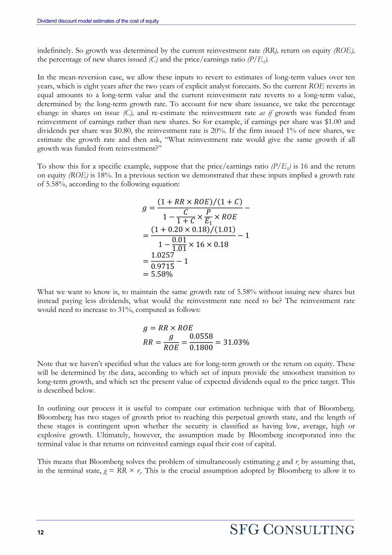
indefinitely. So growth was determined by the current reinvestment rate (RR), return on equity (ROE), the percentage of new shares issued (C) and the price/earnings ratio (P/E1). In the mean-reversion case, we allow these inputs to revert to estimates of long-term values over ten years, which is eight years after the two years of explicit analyst forecasts. So the current ROE reverts in equal amounts to a long-term value and the current reinvestment rate reverts to a long-term value, determined by the long-term growth rate. To account for new share issuance, we take the percentage change in shares on issue (C), and re-estimate the reinvestment rate as if growth was funded from reinvestment of earnings rather than new shares. So for example, if earnings per share was $1.00 and dividends per share was $0.80, the reinvestment rate is 20%. If the firm issued 1% of new shares, we estimate the growth rate and then ask, “What reinvestment rate would give the same growth if all growth was funded from reinvestment?” To show this for a specific example, suppose that the price/earnings ratio (P/E1) is 16 and the return on equity (ROE) is 18%. In a previous section we demonstrated that these inputs implied a growth rate of 5.58%, according to the following equation:
𝑔 =(1 + 𝑅𝑅 × 𝑅𝑂𝐸) (1 + 𝐶)⁄
1 − 𝐶1 + 𝐶 × 𝑃
𝐸1× 𝑅𝑂𝐸
−
=(1 + 0.20 × 0.18) (1.01)⁄
1 − 0.011.01 × 16 × 0.18
− 1
=1.02570.9715
− 1
= 5.58% What we want to know is, to maintain the same growth rate of 5.58% without issuing new shares but instead paying less dividends, what would the reinvestment rate need to be? The reinvestment rate would need to increase to 31%, computed as follows:
𝑔 = 𝑅𝑅 × 𝑅𝑂𝐸
𝑅𝑅 =𝑔
𝑅𝑂𝐸=
0.05580.1800
= 31.03% Note that we haven’t specified what the values are for long-term growth or the return on equity. These will be determined by the data, according to which set of inputs provide the smoothest transition to long-term growth, and which set the present value of expected dividends equal to the price target. This is described below. In outlining our process it is useful to compare our estimation technique with that of Bloomberg. Bloomberg has two stages of growth prior to reaching this perpetual growth state, and the length of these stages is contingent upon whether the security is classified as having low, average, high or explosive growth. Ultimately, however, the assumption made by Bloomberg incorporated into the terminal value is that returns on reinvested earnings equal their cost of capital. This means that Bloomberg solves the problem of simultaneously estimating g and re by assuming that, in the terminal state, g = RR × re. This is the crucial assumption adopted by Bloomberg to allow it to
Dividend discount model estimates of the cost of equity
13
estimate the cost of equity capital for each firm in the market, and for the market risk premium as a market capitalisation-weighted average for all firms.12 The process by which we project dividends and then simultaneously estimate g and re is different on two fronts. The first difference is that we jointly estimate a set of three parameters (long-term growth, cost of equity and long-term return on equity). In contrast, Bloomberg imposes the assumption that the long-term payout ratio is 45% and that long-term returns on equity equal the cost of equity capital.13 In our technique, we consider 2,672 possible combinations of the cost of equity, long-term growth and return on equity. The cost of equity takes on a range of 4% to 20%, long-term ROE takes on a range of 3% to 30% (and which can’t be more than 1% below the cost of equity) and long-term growth takes on a range of 1% to 10% (and which must be less than the cost of equity). We measure ROE according to earnings per share forecasts in year two and book value of equity at the end of year one, and then assume that this return on equity changes incrementally in equal amounts to the long-term ROE estimate. The dividend payout ratio also changes incrementally in equal amounts to the long-term dividend payout ratio, which is equal to 1 – g ÷ ROE. From all combinations of re, g and ROE this allows us to compute 2,672 valuations for each analyst price target, earnings and dividend forecast on each stock. To decide upon the combination of inputs which best fits the data we require that combination to provide a valuation close to average analyst price target and to provide a smooth transition from near-term growth to long-term growth. First, we take all the cases in which the valuation is within 1% of the price target. We then want to know which combination of inputs provides the best fit, or in other words, which is most likely to represent the dividend projections and discount rate incorporated into the valuation. Our criteria is to compare the earnings growth rate in year 10 with the long-term growth rate. We select the case in which the ratio of
12 Note that the cost of equity estimates that Bloomberg reports for individual firms are a combination of dividend discount model estimation and a CAPM estimate. Bloomberg compiles individual firm cost of equity estimates, takes a market capitalisation-weighted average of these estimates to determine the market-wide cost of equity and market risk premium, and then applies its estimate of firm-specific beta to determine each firm’s cost of equity estimate. 13 It is generally-accepted in the accounting literature that accounting standards are conservative, in that accounting earnings and balance sheet values have more chance of being understated than overstated (Cheng, 2005; Easton, 2006). So whether return on equity (NPAT/Equity) has more chance of being overstated or understated depends upon whether those conservative accounting assumptions have a relatively greater impact on the income statement or the balance sheet. This means that we can observe return on equity which exceeds the cost of equity capital even if, in economic substance, that economic rents are zero. In relation to conservative accounting assumptions, Cheng cites the example of research and development expenditure being expensed, even though this expenditure is expected to generate future economic benefits. In relation to economic rents, Cheng states that the absence of perfect competition can mean that some firms can set prices above their marginal costs and generate abnormal earnings. The key points are (1) that we do observe return on equity in historical data which exceeds the cost of equity capital, (2) there are reasons why we would not necessarily expect the return on equity and the cost of equity capital to converge, and (3) that we are able to estimate the cost of equity capital without imposing the assumption that it equals the return on equity. The assumption that long-term returns on investment equal the cost of capital is also invoked by Li, Ng and Swaminathan (2013), who implement this assumption after a 15-year forecast horizon. The typical price/earnings ratio in their sample is around 14 and, as we discuss later, if returns equal the cost of capital the long-term price/earnings ratio will be the inverse of the cost of capital. So under most cost of capital estimates price/earnings ratios will decline to single digits. An initial price/earnings ratio of 14 and a long-term price/earnings ratio below 10 is only possible with very high dividend and earnings growth initially, falling rapidly to long-term growth.
Dividend discount model estimates of the cost of equity
14
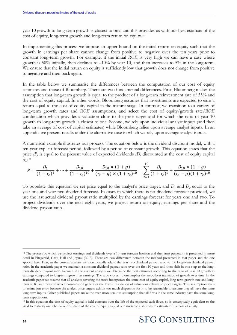
year 10 growth to long-term growth is closest to one, and this provides us with our best estimate of the cost of equity, long-term growth and long-term return on equity.14 In implementing this process we impose an upper bound on the initial return on equity such that the growth in earnings per share cannot change from positive to negative over the ten years prior to constant long-term growth. For example, if the initial ROE is very high we can have a case where growth is 50% initially, then declines to –10% by year 10, and then increases to 5% in the long-term. We ensure that the initial return on equity is sufficiently low that growth does not change from positive to negative and then back again. In the table below we summarise the differences between the computation of our cost of equity estimates and those of Bloomberg. There are two fundamental differences. First, Bloomberg makes the assumption that long-term growth is equal to the product of a long-term reinvestment rate of 55% and the cost of equity capital. In other words, Bloomberg assumes that investments are expected to earn a return equal to the cost of equity capital in the mature stage. In contrast, we transition to a variety of long-term growth rates and ROE assumptions, and select the cost of equity/growth rate/ROE combination which provides a valuation close to the price target and for which the ratio of year 10 growth to long-term growth is closest to one. Second, we rely upon individual analyst inputs (and then take an average of cost of capital estimates) while Bloomberg relies upon average analyst inputs. In an appendix we present results under the alternative case in which we rely upon average analyst inputs. A numerical example illustrates our process. The equation below is the dividend discount model, with a ten-year explicit forecast period, followed by a period of constant growth. This equation states that the price (P) is equal to the present value of expected dividends (D) discounted at the cost of equity capital (re).15
𝑃 =𝐷1
(1 + 𝑟𝑒)1 + ⋯ +𝐷10
(1 + 𝑟𝑒)10 +𝐷10 × (1 + 𝑔)
(𝑟𝑒 − 𝑔) × (1 + 𝑟𝑒)10 = �𝐷𝑡
(1 + 𝑟𝑒)𝑡 +𝐷10 × (1 + 𝑔)
(𝑟𝑒 − 𝑔)(1 + 𝑟𝑒)10
10
𝑡=1
To populate this equation we set price equal to the analyst’s price target, and D1 and D2 equal to the year one and year two dividend forecast. In cases in which there is no dividend forecast provided, we use the last actual dividend payout ratio multiplied by the earnings forecast for years one and two. To project dividends over the next eight years, we project return on equity, earnings per share and the dividend payout ratio.
14 The process by which we project earnings and dividends over a 10 year forecast horizon and then into perpetuity is presented in more detail in Fitzgerald, Gray, Hall and Jeyaraj (2013). There are two differences between the method presented in that paper and the one applied here. First, in the current analysis we incrementally adjust the year two dividend payout ratio to the long-term dividend payout ratio. In the academic paper we maintain a constant dividend payout ratio over the first 10 years and then shift in one step to the long-term dividend payout ratio. Second, in the current analysis we determine the best estimates according to the ratio of year 10 growth in earnings compared to long-term growth in earnings. The ratio closest to one implies the smoothest transition of growth over time. In the academic paper we assume that all analysts covering the stock incorporate the same cost of equity capital, long-term growth rate and long-term ROE and measure which combination generates the lowest dispersion of valuations relative to price targets. This assumption leads to estimation error because the analyst price targets exhibit too much dispersion for it to be reasonable to assume they all have the same long-term inputs. Other published papers make the even more tenuous assumption that all firms in the same industry have the same long-term expectations. 15 In this equation the cost of equity capital is held constant over the life of the expected cash flows, so is conceptually equivalent to the yield to maturity on debt. So our estimate of the cost of equity capital is in no sense a short-term estimate of the cost of equity.
Dividend discount model estimates of the cost of equity
15
Table 1. Comparison between SFG and Bloomberg estimates of the cost of equity SFG Bloomberg
Time period prior to constant/mature growth
10 years 19 years
What is the ROE at maturity?
3% to 30% re
What is the dividend payout ratio at maturity?
1 – g ÷ ROE 45%
What is the constant growth rate at maturity?
1% to 10% (1 – DPR) × re
How to transition to long-term growth?
Explicit forecasts of dividends and earnings in years 1 and 2.
ROE in year 2 reverts to long-term ROE over remaining 8 years.
DPR in year 2 reverts to long-term DPR over remaining 8 years.
Reversion is in equal increments.
Explicit forecasts of dividends and earnings in years 1 and 2.
“Growth” stage of either 3, 5, 7 or 9 years.
“Transition” stage of either 14, 12, 10 or 8 years.
Length of stages contingent upon Bloomberg’s classification of the firm into explosive, high, average or slow growth. This classification is based upon the distribution of growth rates for all firms.
Growth rate during “growth” stage is analyst’s average estimate of long-term growth.
Reversion in equal increments to mature growth rate over transition stage.
Data Individual analyst inputs for each firm over a six month period. Earnings and dividend expectations matched with price target.
On each date, average values computed for all outstanding analyst inputs available at that data. Earnings and dividend expectations matched with share price.
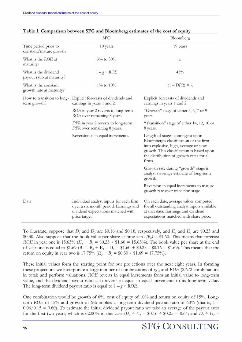
To illustrate, suppose that D1 and D2 are $0.16 and $0.18, respectively, and E1 and E2 are $0.25 and $0.30. Also suppose that the book value per share at time zero (B0) is $1.60. This means that forecast ROE in year one is 15.63% (E1 ÷ B0 = $0.25 ÷ $1.60 = 15.63%). The book value per share at the end of year one is equal to $1.69 (B1 = B0 + E1 – D1 = $1.60 + $0.25 – $0.16 = $1.69). This means that the return on equity in year two is 17.75% (E2 ÷ B1 = $0.30 ÷ $1.69 = 17.75%). These initial values form the starting point for our projections over the next eight years. In forming these projections we incorporate a large number of combinations of re, g and ROE (2,672 combinations in total) and perform valuations. ROE reverts in equal increments from an initial value to long-term value, and the dividend payout ratio also reverts in equal in equal increments to its long-term value. The long-term dividend payout ratio is equal to 1 – g ÷ ROE. One combination would be growth of 6%, cost of equity of 10% and return on equity of 15%. Long-term ROE of 15% and growth of 6% implies a long-term dividend payout ratio of 60% (that is, 1 – 0.06/0.15 = 0.60). To estimate the initial dividend payout ratio we take an average of the payout ratio for the first two years, which is 62.00% in this case (D1 ÷ E1 = $0.16 ÷ $0.25 = 0.64; and D2 ÷ E2 =
Dividend discount model estimates of the cost of equity
16
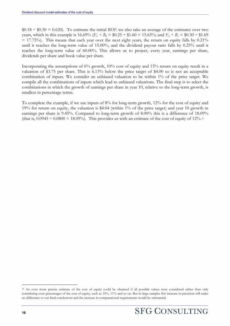
$0.18 ÷ $0.30 = 0.620). To estimate the initial ROE we also take an average of the estimates over two years, which in this example is 16.69% (E1 ÷ B0 = $0.25 ÷ $1.60 = 15.63%; and E2 ÷ B1 = $0.30 ÷ $1.69 = 17.75%). This means that each year over the next eight years, the return on equity falls by 0.21% until it reaches the long-term value of 15.00%, and the dividend payout ratio falls by 0.25% until it reaches the long-term value of 60.00%. This allows us to project, every year, earnings per share, dividends per share and book value per share. Incorporating the assumptions of 6% growth, 10% cost of equity and 15% return on equity result in a valuation of $3.75 per share. This is 6.13% below the price target of $4.00 so is not an acceptable combination of inputs. We consider an unbiased valuation to be within 1% of the price target. We compile all the combinations of inputs which lead to unbiased valuations. The final step is to select the combinations in which the growth of earnings per share in year 10, relative to the long-term growth, is smallest in percentage terms. To complete the example, if we use inputs of 8% for long-term growth, 12% for the cost of equity and 19% for return on equity, the valuation is $4.04 (within 1% of the price target) and year 10 growth in earnings per share is 9.45%. Compared to long-term growth of 8.00% this is a difference of 18.09% (that is, 0.0945 ÷ 0.0800 = 18.09%). This provides us with an estimate of the cost of equity of 12%.16
16 An even more precise estimate of the cost of equity could be obtained if all possible values were considered rather than only considering even percentages of the cost of equity, such as 10%, 11% and so on. But in large samples this increase in precision will make no difference to our final conclusions and the increase in computational requirements would be substantial.
Dividend discount model estimates of the cost of equity
17
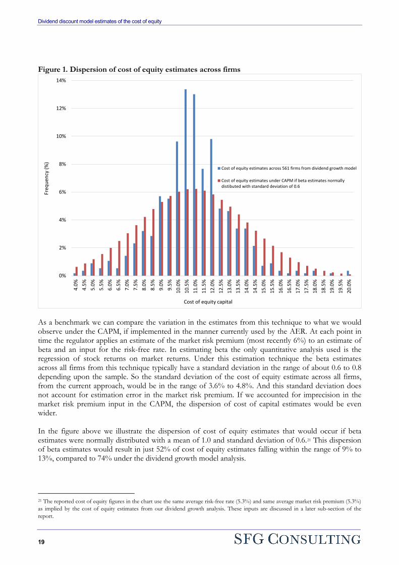
4. Results 4.1 Data The total number of analyst inputs in the IBES dataset which had sufficient data available for analysis was 39,564. This means that over the 10.5 year period there were just under 40,000 combinations of earnings per share expectations, dividends per share expectations and price targets for Australian-listed firms with all other data available for analysis. We partitioned the sample into six month intervals so we have a large number of firms and analyst inputs available in every six month period. An individual analyst can make more than one input for each firm in a six month period. For each of the 39,564 observations we estimate the cost of equity capital, and average these estimates across all analyst inputs for each firm every six months. This allows us to compile a sample of 4,567 estimates of firm cost of equity estimates. On average, each time a firm appears in a six month period, there are 8.7 cost of equity estimates for that firm. There are also 561 individual firms in the dataset which means that, on average, each firm appears in the dataset 8.1 times over the 10.5 year period. There were 31 firms that appeared in the sample in all 21 half-year periods. These firms include 13 firms in the ASX20. On average, firms in the ASX20 appeared in the sample in 19.8 periods, firms previously used by the regulator in benchmarking appeared in the sample in 9.4 periods and the remaining 532 firms appeared in the sample in 7.7 periods. Across the 4,567 sample firm/half-years, we have the following average values – dividend yield of 4.6%, price/earnings ratio of 18.017, initial return on equity of 17.5% and change in shares on issue of 1.7%. For the analysis incorporating constant growth the average initial return on equity is 22.7%. This lower average return on equity under mean reversion results from the constraint on initial growth which prevents growth switching from positive to negative to positive again. Also note that, on average, analyst price targets are 14% higher than share prices. So if we were to use share prices in our analysis, the cost of equity estimates would be higher than we present here. 4.2 Estimates assuming mean-reversion in parameter inputs 4.2.1 Individual firms In Table 2 we summarise our estimates for individual firms, assuming mean-reversion in parameter inputs. We present results for all firm/half-years, for 85 cases pertaining to the Australian-listed network businesses previously analysed by the regulator, and for the non-network firms. In the subsequent table we present results on an industry basis. It should be emphasised that the results presented in this table are for the average Australian-listed firm over the period 2H02 to 2H12. They are not estimates of the cost of capital at the end of 2012. Across all observations the average cost of equity is 10.8% and the standard deviation is 2.4%. This is slightly different to the cost of equity for the market, which we discuss subsequently. For the market cost of equity, as an input into asset pricing models, we compute a market capitalisation-weighted average cost of equity over time.
17 These dividend yield values and price/earnings ratios are based upon price targets. If we compute the price/earnings ratio on the basis of the share price, rather than the price target, the average price/earnings ratio is 16.0 and the average dividend yield is 5.1%.
Dividend discount model estimates of the cost of equity
18
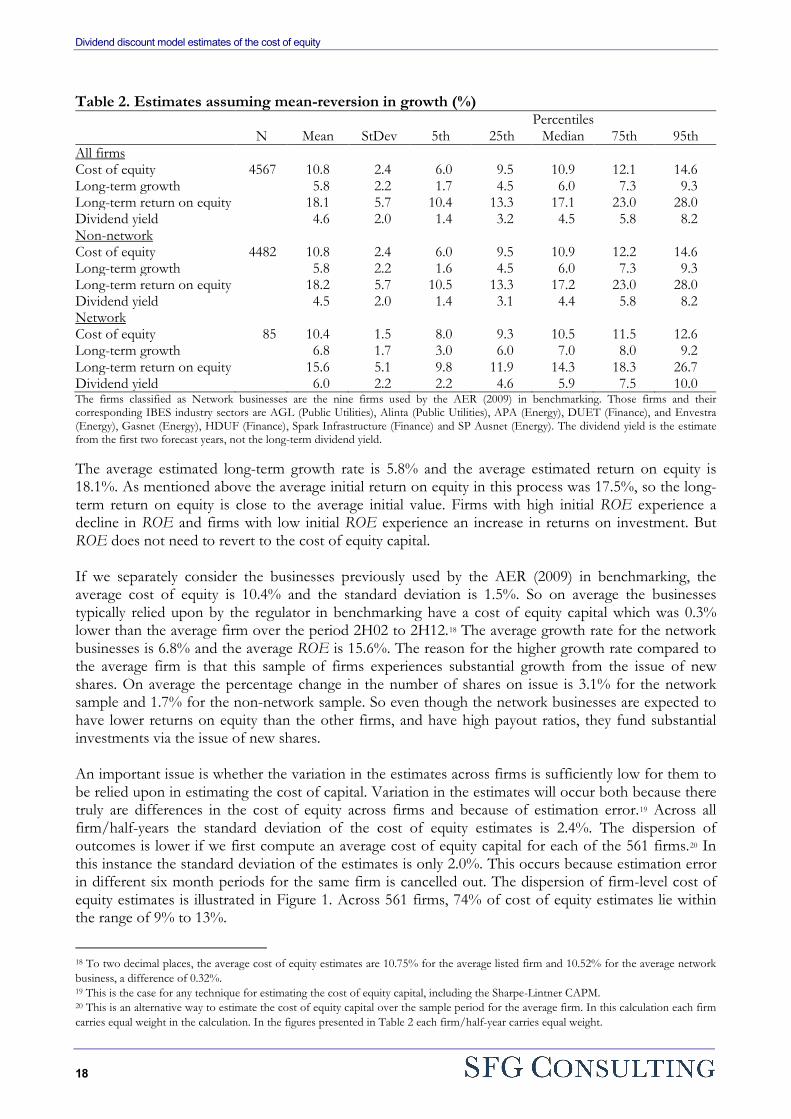
Table 2. Estimates assuming mean-reversion in growth (%) Percentiles N Mean StDev 5th 25th Median 75th 95th
All firms Cost of equity 4567 10.8 2.4 6.0 9.5 10.9 12.1 14.6 Long-term growth 5.8 2.2 1.7 4.5 6.0 7.3 9.3 Long-term return on equity 18.1 5.7 10.4 13.3 17.1 23.0 28.0 Dividend yield 4.6 2.0 1.4 3.2 4.5 5.8 8.2 Non-network Cost of equity 4482 10.8 2.4 6.0 9.5 10.9 12.2 14.6 Long-term growth 5.8 2.2 1.6 4.5 6.0 7.3 9.3 Long-term return on equity 18.2 5.7 10.5 13.3 17.2 23.0 28.0 Dividend yield 4.5 2.0 1.4 3.1 4.4 5.8 8.2 Network Cost of equity 85 10.4 1.5 8.0 9.3 10.5 11.5 12.6 Long-term growth 6.8 1.7 3.0 6.0 7.0 8.0 9.2 Long-term return on equity 15.6 5.1 9.8 11.9 14.3 18.3 26.7 Dividend yield 6.0 2.2 2.2 4.6 5.9 7.5 10.0 The firms classified as Network businesses are the nine firms used by the AER (2009) in benchmarking. Those firms and their corresponding IBES industry sectors are AGL (Public Utilities), Alinta (Public Utilities), APA (Energy), DUET (Finance), and Envestra (Energy), Gasnet (Energy), HDUF (Finance), Spark Infrastructure (Finance) and SP Ausnet (Energy). The dividend yield is the estimate from the first two forecast years, not the long-term dividend yield. The average estimated long-term growth rate is 5.8% and the average estimated return on equity is 18.1%. As mentioned above the average initial return on equity in this process was 17.5%, so the long-term return on equity is close to the average initial value. Firms with high initial ROE experience a decline in ROE and firms with low initial ROE experience an increase in returns on investment. But ROE does not need to revert to the cost of equity capital. If we separately consider the businesses previously used by the AER (2009) in benchmarking, the average cost of equity is 10.4% and the standard deviation is 1.5%. So on average the businesses typically relied upon by the regulator in benchmarking have a cost of equity capital which was 0.3% lower than the average firm over the period 2H02 to 2H12.18 The average growth rate for the network businesses is 6.8% and the average ROE is 15.6%. The reason for the higher growth rate compared to the average firm is that this sample of firms experiences substantial growth from the issue of new shares. On average the percentage change in the number of shares on issue is 3.1% for the network sample and 1.7% for the non-network sample. So even though the network businesses are expected to have lower returns on equity than the other firms, and have high payout ratios, they fund substantial investments via the issue of new shares. An important issue is whether the variation in the estimates across firms is sufficiently low for them to be relied upon in estimating the cost of capital. Variation in the estimates will occur both because there truly are differences in the cost of equity across firms and because of estimation error.19 Across all firm/half-years the standard deviation of the cost of equity estimates is 2.4%. The dispersion of outcomes is lower if we first compute an average cost of equity capital for each of the 561 firms.20 In this instance the standard deviation of the estimates is only 2.0%. This occurs because estimation error in different six month periods for the same firm is cancelled out. The dispersion of firm-level cost of equity estimates is illustrated in Figure 1. Across 561 firms, 74% of cost of equity estimates lie within the range of 9% to 13%.
18 To two decimal places, the average cost of equity estimates are 10.75% for the average listed firm and 10.52% for the average network business, a difference of 0.32%. 19 This is the case for any technique for estimating the cost of equity capital, including the Sharpe-Lintner CAPM. 20 This is an alternative way to estimate the cost of equity capital over the sample period for the average firm. In this calculation each firm carries equal weight in the calculation. In the figures presented in Table 2 each firm/half-year carries equal weight.
Dividend discount model estimates of the cost of equity
19
Figure 1. Dispersion of cost of equity estimates across firms
As a benchmark we can compare the variation in the estimates from this technique to what we would observe under the CAPM, if implemented in the manner currently used by the AER. At each point in time the regulator applies an estimate of the market risk premium (most recently 6%) to an estimate of beta and an input for the risk-free rate. In estimating beta the only quantitative analysis used is the regression of stock returns on market returns. Under this estimation technique the beta estimates across all firms from this technique typically have a standard deviation in the range of about 0.6 to 0.8 depending upon the sample. So the standard deviation of the cost of equity estimate across all firms, from the current approach, would be in the range of 3.6% to 4.8%. And this standard deviation does not account for estimation error in the market risk premium. If we accounted for imprecision in the market risk premium input in the CAPM, the dispersion of cost of capital estimates would be even wider. In the figure above we illustrate the dispersion of cost of equity estimates that would occur if beta estimates were normally distributed with a mean of 1.0 and standard deviation of 0.6.21 This dispersion of beta estimates would result in just 52% of cost of equity estimates falling within the range of 9% to 13%, compared to 74% under the dividend growth model analysis.
21 The reported cost of equity figures in the chart use the same average risk-free rate (5.3%) and same average market risk premium (5.3%) as implied by the cost of equity estimates from our dividend growth analysis. These inputs are discussed in a later sub-section of the report.
0%
2%
4%
6%
8%
10%
12%
14%4.
0%4.
5%5.
0%5.
5%6.
0%6.
5%7.
0%7.
5%8.
0%8.
5%9.
0%9.
5%10
.0%
10.5
%11
.0%
11.5
%12
.0%
12.5
%13
.0%
13.5
%14
.0%
14.5
%15
.0%
15.5
%16
.0%
16.5
%17
.0%
17.5
%18
.0%
18.5
%19
.0%
19.5
%20
.0%
Freq
uenc
y (%
)
Cost of equity capital
Cost of equity estimates across 561 firms from dividend growth model
Cost of equity estimates under CAPM if beta estimates normallydistibuted with standard deviation of 0.6
Dividend discount model estimates of the cost of equity
20
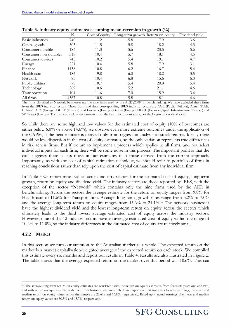
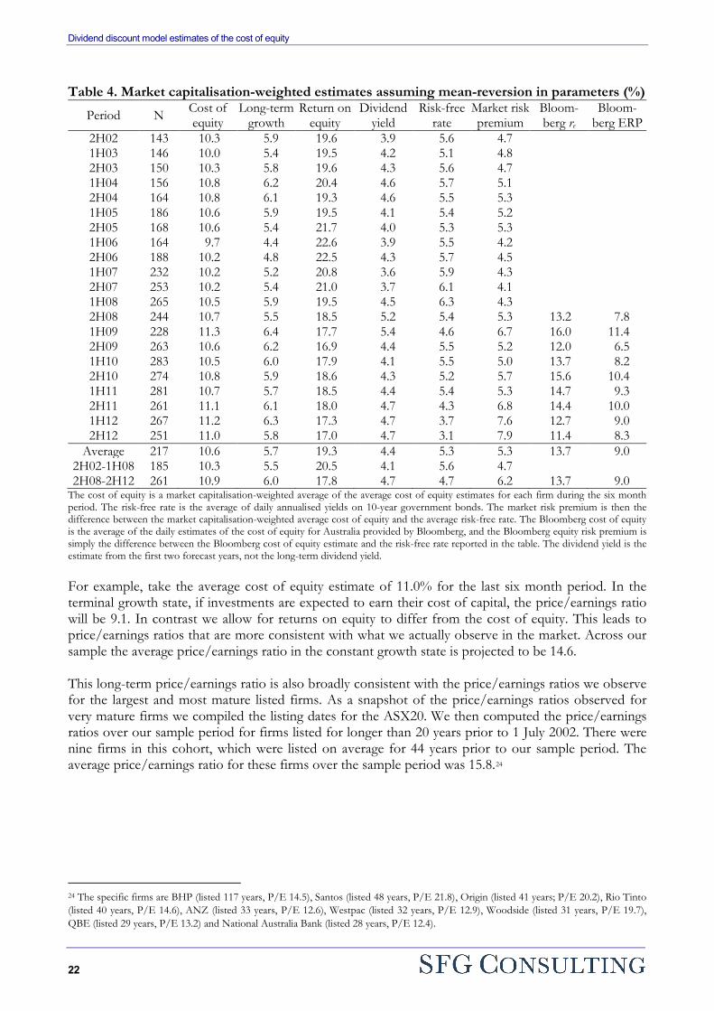
Table 3. Industry equity estimates assuming mean-reversion in growth (%) N Cost of equity Long-term growth Return on equity Dividend yield Basic industries 740 11.2 5.8 17.9 3.6 Capital goods 503 11.5 5.8 18.2 4.3 Consumer durables 183 11.0 5.6 20.5 5.6 Consumer non-durables 318 10.4 5.7 18.1 4.5 Consumer services 745 10.2 5.4 19.1 4.7 Energy 221 10.4 5.8 17.9 3.1 Finance 1138 10.8 6.2 16.7 5.4 Health care 183 9.8 6.0 18.2 3.5 Network 85 10.4 6.8 15.6 6.0 Public utilities 78 10.7 5.4 20.8 5.4 Technology 269 10.6 5.2 21.1 4.6 Transportation 104 11.6 7.0 15.9 3.4 All firms 4567 10.8 5.8 18.1 4.6 The firms classified as Network businesses are the nine firms used by the AER (2009) in benchmarking. We have excluded these firms from the IBES industry sectors. Those firms and their corresponding IBES industry sectors are AGL (Public Utilities), Alinta (Public Utilities), APA (Energy), DUET (Finance), and Envestra (Energy), Gasnet (Energy), HDUF (Finance), Spark Infrastructure (Finance) and SP Ausnet (Energy). The dividend yield is the estimate from the first two forecast years, not the long-term dividend yield. So while there are some high and low values for the estimated cost of equity (10% of outcomes are either below 6.0% or above 14.6%), we observe even more extreme outcomes under the application of the CAPM, if the beta estimate is derived only from regression analysis of stock returns. Ideally there would be less dispersion in the cost of equity estimates, so the only variation represents true differences in risk across firms. But if we are to implement a process which applies to all firms, and not select individual inputs for each firm, there will be some noise in this process. The important point is that the data suggests there is less noise in our estimates than those derived from the current approach. Importantly, as with any cost of capital estimation technique, we should refer to portfolio of firms in reaching conclusions rather than rely upon the cost of capital estimate from any individual firm. In Table 3 we report mean values across industry sectors for the estimated cost of equity, long-term growth, return on equity and dividend yield. The industry sectors are those reported by IBES, with the exception of the sector “Network” which contains only the nine firms used by the AER in benchmarking. Across the sectors the average estimate for the return on equity ranges from 9.8% for Health care to 11.6% for Transportation. Average long-term growth rates range from 5.2% to 7.0% and the average long-term return on equity ranges from 15.6% to 21.1%.22 The network businesses have the highest dividend yield and the lowest long-term return on equity across the sectors which ultimately leads to the third lowest average estimated cost of equity across the industry sectors. However, nine of the 12 industry sectors have an average estimated cost of equity within the range of 10.2% to 11.0%, so the industry differences in the estimated cost of equity are relatively small. 4.2.2 Market In this section we turn our attention to the Australian market as a whole. The expected return on the market is a market capitalisation-weighted average of the expected return on each stock. We compiled this estimate every six months and report our results in Table 4. Results are also illustrated in Figure 2. The table shows that the average expected return on the market over this period was 10.6%. This can
22 The average long-term return on equity estimates are consistent with the return on equity estimates from forecasts years one and two, and with return on equity estimates derived from historical earnings only. Based upon the first two years forecast earnings, the mean and median return on equity values across the sample are 22.6% and 16.9%, respectively. Based upon actual earnings, the mean and median return on equity values are 30.5% and 15.7%, respectively.
Dividend discount model estimates of the cost of equity
21
be compared to the 5.3% average yield on 10 year government bonds to form an estimate of the market risk premium over this period. The average market risk premium over this period is estimated at 5.3%.23 The global financial crisis began to materially impact asset prices in the second half of 2008, following which we observed substantial increases in corporate debt yields and decreases in the yield on government bonds. In our sample we also observe an increase in the estimated market cost of equity during this period. From 2H02 to 1H08 the average cost of equity for the market was 10.3%, which increased to an average 10.9% from 2H08 to 2H12. In comparison to a declining risk-free rate, the estimated market risk premium rose from an average 4.7% to 6.2%. In the last six months of the sample the market risk premium is estimated at 7.9%. This is the most recent data in the sample so our estimate of the prevailing market cost of equity is 11.0% and the implied market risk premium is 7.9%. The estimates provided by Bloomberg provide a point of comparison. Bloomberg estimates are only available from the second half of 2008 onwards. On average the expected return on the market from Bloomberg is 13.7% from 2H08 to 2H12 (compared to our estimate of 10.9%) and the average implied market risk premium is 9.0% (compared to our estimate of 6.0%). The Bloomberg approach incorporates higher growth assumptions, especially in the short term, which leads to a higher estimated cost of equity capital. The Bloomberg process for transitioning from initial growth to long-term growth is summarised in Table 1. In the long term, the approach adopted by Bloomberg means that investments earn their cost of capital. So ultimately the estimates compiled by Bloomberg will lead to price/earnings ratios that are the inverse of the cost of equity capital. To see why this is the case, consider the equation for price in a constant growth state:
𝑃 =𝐷1
𝑟𝑒 − 𝑔=
𝐷1
𝑟𝑒 − 𝑅𝑅 × 𝑅𝑂𝐸
If the return on equity (ROE) is set equal to the cost of equity (re) then we have:
𝑃 =𝐷1
𝑟𝑒 − 𝑔=
𝐷1
𝑟𝑒 − 𝑅𝑅 × 𝑟𝑒
Then if we set the reinvestment rate equal to (1 – Dividend payout ratio = 1 – D1/E1) we can solve for the price/earnings ratio:
𝑃 =𝐷1
𝑟𝑒 − (1 − 𝐷1 𝐸1⁄ ) × 𝑟𝑒
=𝐷1
𝑟𝑒 − 𝑟𝑒 + 𝐷1 𝐸1 × 𝑟𝑒⁄
=𝐷1
𝐷1 𝐸1 × 𝑟𝑒⁄
𝑃𝐸1
=1𝑟𝑒
23 We reiterate that this estimate of the market risk premium does not include any tax benefits of imputation or other tax benefits. It represents the market risk premium from dividends and capital gains only.
Dividend discount model estimates of the cost of equity
22
Table 4. Market capitalisation-weighted estimates assuming mean-reversion in parameters (%)
Period N Cost of equity
Long-term growth
Return on equity
Dividend yield
Risk-free rate
Market risk premium
Bloom-berg re
Bloom-berg ERP
2H02 143 10.3 5.9 19.6 3.9 5.6 4.7 1H03 146 10.0 5.4 19.5 4.2 5.1 4.8 2H03 150 10.3 5.8 19.6 4.3 5.6 4.7 1H04 156 10.8 6.2 20.4 4.6 5.7 5.1 2H04 164 10.8 6.1 19.3 4.6 5.5 5.3 1H05 186 10.6 5.9 19.5 4.1 5.4 5.2 2H05 168 10.6 5.4 21.7 4.0 5.3 5.3 1H06 164 9.7 4.4 22.6 3.9 5.5 4.2 2H06 188 10.2 4.8 22.5 4.3 5.7 4.5 1H07 232 10.2 5.2 20.8 3.6 5.9 4.3 2H07 253 10.2 5.4 21.0 3.7 6.1 4.1 1H08 265 10.5 5.9 19.5 4.5 6.3 4.3 2H08 244 10.7 5.5 18.5 5.2 5.4 5.3 13.2 7.8 1H09 228 11.3 6.4 17.7 5.4 4.6 6.7 16.0 11.4 2H09 263 10.6 6.2 16.9 4.4 5.5 5.2 12.0 6.5 1H10 283 10.5 6.0 17.9 4.1 5.5 5.0 13.7 8.2 2H10 274 10.8 5.9 18.6 4.3 5.2 5.7 15.6 10.4 1H11 281 10.7 5.7 18.5 4.4 5.4 5.3 14.7 9.3 2H11 261 11.1 6.1 18.0 4.7 4.3 6.8 14.4 10.0 1H12 267 11.2 6.3 17.3 4.7 3.7 7.6 12.7 9.0 2H12 251 11.0 5.8 17.0 4.7 3.1 7.9 11.4 8.3
Average 217 10.6 5.7 19.3 4.4 5.3 5.3 13.7 9.0 2H02-1H08 185 10.3 5.5 20.5 4.1 5.6 4.7 2H08-2H12 261 10.9 6.0 17.8 4.7 4.7 6.2 13.7 9.0
The cost of equity is a market capitalisation-weighted average of the average cost of equity estimates for each firm during the six month period. The risk-free rate is the average of daily annualised yields on 10-year government bonds. The market risk premium is then the difference between the market capitalisation-weighted average cost of equity and the average risk-free rate. The Bloomberg cost of equity is the average of the daily estimates of the cost of equity for Australia provided by Bloomberg, and the Bloomberg equity risk premium is simply the difference between the Bloomberg cost of equity estimate and the risk-free rate reported in the table. The dividend yield is the estimate from the first two forecast years, not the long-term dividend yield. For example, take the average cost of equity estimate of 11.0% for the last six month period. In the terminal growth state, if investments are expected to earn their cost of capital, the price/earnings ratio will be 9.1. In contrast we allow for returns on equity to differ from the cost of equity. This leads to price/earnings ratios that are more consistent with what we actually observe in the market. Across our sample the average price/earnings ratio in the constant growth state is projected to be 14.6. This long-term price/earnings ratio is also broadly consistent with the price/earnings ratios we observe for the largest and most mature listed firms. As a snapshot of the price/earnings ratios observed for very mature firms we compiled the listing dates for the ASX20. We then computed the price/earnings ratios over our sample period for firms listed for longer than 20 years prior to 1 July 2002. There were nine firms in this cohort, which were listed on average for 44 years prior to our sample period. The average price/earnings ratio for these firms over the sample period was 15.8.24
24 The specific firms are BHP (listed 117 years, P/E 14.5), Santos (listed 48 years, P/E 21.8), Origin (listed 41 years; P/E 20.2), Rio Tinto (listed 40 years, P/E 14.6), ANZ (listed 33 years, P/E 12.6), Westpac (listed 32 years, P/E 12.9), Woodside (listed 31 years, P/E 19.7), QBE (listed 29 years, P/E 13.2) and National Australia Bank (listed 28 years, P/E 12.4).
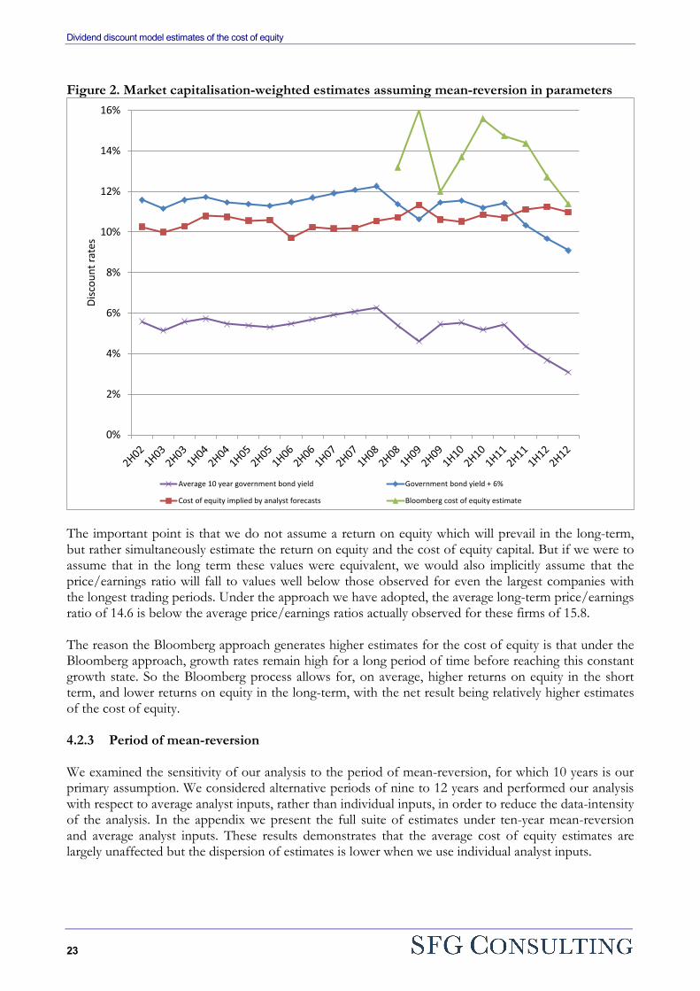
Dividend discount model estimates of the cost of equity
23
Figure 2. Market capitalisation-weighted estimates assuming mean-reversion in parameters
The important point is that we do not assume a return on equity which will prevail in the long-term, but rather simultaneously estimate the return on equity and the cost of equity capital. But if we were to assume that in the long term these values were equivalent, we would also implicitly assume that the price/earnings ratio will fall to values well below those observed for even the largest companies with the longest trading periods. Under the approach we have adopted, the average long-term price/earnings ratio of 14.6 is below the average price/earnings ratios actually observed for these firms of 15.8. The reason the Bloomberg approach generates higher estimates for the cost of equity is that under the Bloomberg approach, growth rates remain high for a long period of time before reaching this constant growth state. So the Bloomberg process allows for, on average, higher returns on equity in the short term, and lower returns on equity in the long-term, with the net result being relatively higher estimates of the cost of equity. 4.2.3 Period of mean-reversion We examined the sensitivity of our analysis to the period of mean-reversion, for which 10 years is our primary assumption. We considered alternative periods of nine to 12 years and performed our analysis with respect to average analyst inputs, rather than individual inputs, in order to reduce the data-intensity of the analysis. In the appendix we present the full suite of estimates under ten-year mean-reversion and average analyst inputs. These results demonstrates that the average cost of equity estimates are largely unaffected but the dispersion of estimates is lower when we use individual analyst inputs.
0%
2%
4%
6%
8%
10%
12%
14%
16%
Disc
ount
rate
s
Average 10 year government bond yield Government bond yield + 6%
Cost of equity implied by analyst forecasts Bloomberg cost of equity estimate
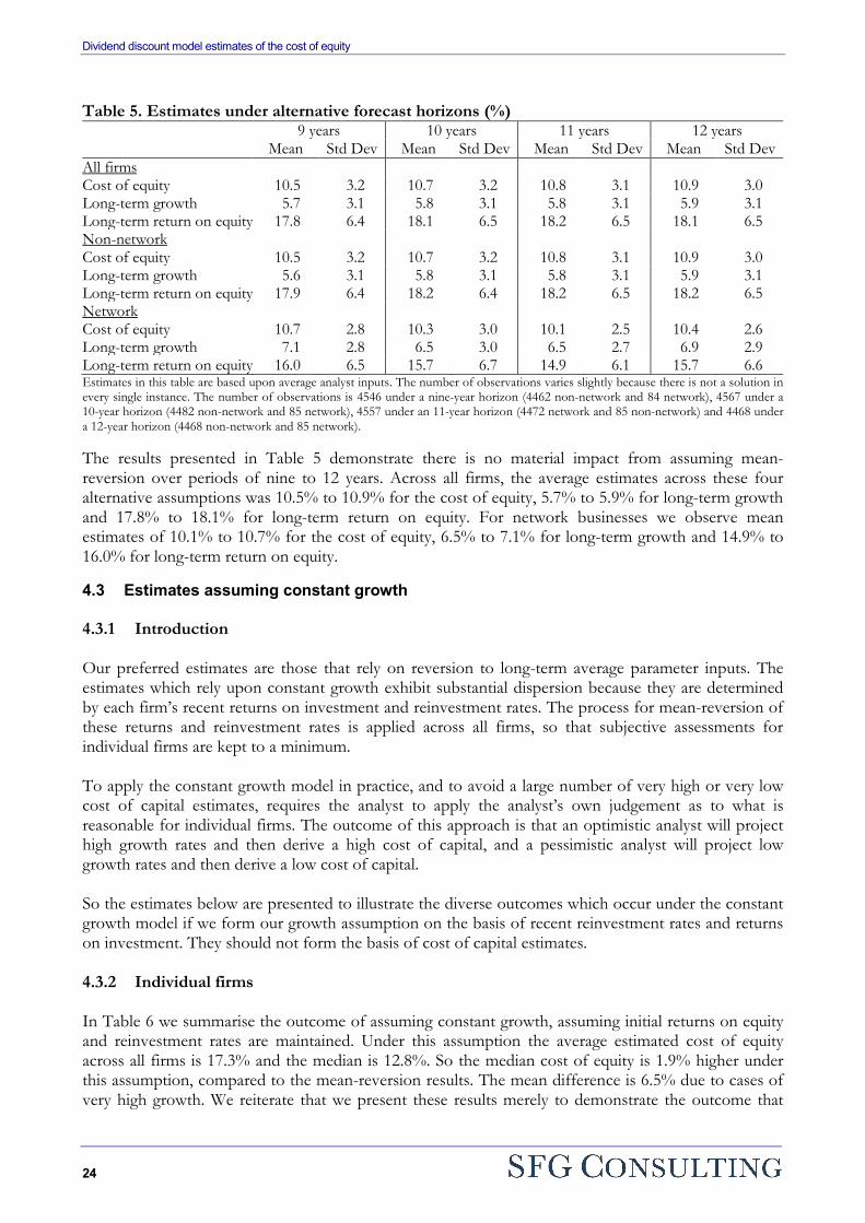
Dividend discount model estimates of the cost of equity
24
Table 5. Estimates under alternative forecast horizons (%) 9 years 10 years 11 years 12 years Mean Std Dev Mean Std Dev Mean Std Dev Mean Std Dev All firms Cost of equity 10.5 3.2 10.7 3.2 10.8 3.1 10.9 3.0 Long-term growth 5.7 3.1 5.8 3.1 5.8 3.1 5.9 3.1 Long-term return on equity 17.8 6.4 18.1 6.5 18.2 6.5 18.1 6.5 Non-network Cost of equity 10.5 3.2 10.7 3.2 10.8 3.1 10.9 3.0 Long-term growth 5.6 3.1 5.8 3.1 5.8 3.1 5.9 3.1 Long-term return on equity 17.9 6.4 18.2 6.4 18.2 6.5 18.2 6.5 Network Cost of equity 10.7 2.8 10.3 3.0 10.1 2.5 10.4 2.6 Long-term growth 7.1 2.8 6.5 3.0 6.5 2.7 6.9 2.9 Long-term return on equity 16.0 6.5 15.7 6.7 14.9 6.1 15.7 6.6 Estimates in this table are based upon average analyst inputs. The number of observations varies slightly because there is not a solution in every single instance. The number of observations is 4546 under a nine-year horizon (4462 non-network and 84 network), 4567 under a 10-year horizon (4482 non-network and 85 network), 4557 under an 11-year horizon (4472 network and 85 non-network) and 4468 under a 12-year horizon (4468 non-network and 85 network). The results presented in Table 5 demonstrate there is no material impact from assuming mean-reversion over periods of nine to 12 years. Across all firms, the average estimates across these four alternative assumptions was 10.5% to 10.9% for the cost of equity, 5.7% to 5.9% for long-term growth and 17.8% to 18.1% for long-term return on equity. For network businesses we observe mean estimates of 10.1% to 10.7% for the cost of equity, 6.5% to 7.1% for long-term growth and 14.9% to 16.0% for long-term return on equity. 4.3 Estimates assuming constant growth 4.3.1 Introduction Our preferred estimates are those that rely on reversion to long-term average parameter inputs. The estimates which rely upon constant growth exhibit substantial dispersion because they are determined by each firm’s recent returns on investment and reinvestment rates. The process for mean-reversion of these returns and reinvestment rates is applied across all firms, so that subjective assessments for individual firms are kept to a minimum. To apply the constant growth model in practice, and to avoid a large number of very high or very low cost of capital estimates, requires the analyst to apply the analyst’s own judgement as to what is reasonable for individual firms. The outcome of this approach is that an optimistic analyst will project high growth rates and then derive a high cost of capital, and a pessimistic analyst will project low growth rates and then derive a low cost of capital. So the estimates below are presented to illustrate the diverse outcomes which occur under the constant growth model if we form our growth assumption on the basis of recent reinvestment rates and returns on investment. They should not form the basis of cost of capital estimates. 4.3.2 Individual firms In Table 6 we summarise the outcome of assuming constant growth, assuming initial returns on equity and reinvestment rates are maintained. Under this assumption the average estimated cost of equity across all firms is 17.3% and the median is 12.8%. So the median cost of equity is 1.9% higher under this assumption, compared to the mean-reversion results. The mean difference is 6.5% due to cases of very high growth. We reiterate that we present these results merely to demonstrate the outcome that
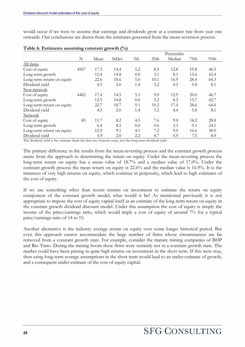
Dividend discount model estimates of the cost of equity
25
would occur if we were to assume that earnings and dividends grow at a constant rate from year one onwards. Our conclusions are drawn from the estimates generated from the mean-reversion process. Table 6. Estimates assuming constant growth (%)
Percentiles N Mean StDev 5th 25th Median 75th 95th
All firms Cost of equity 4567 17.3 14.4 5.2 8.9 12.8 19.8 46.5 Long-term growth 12.4 14.8 0.0 3.1 8.1 15.6 42.4 Long-term return on equity 22.6 18.6 5.0 10.1 16.9 28.4 64.3 Dividend yield 4.5 2.0 1.4 3.2 4.5 5.8 8.1 Non-network Cost of equity 4482 17.4 14.5 5.3 9.0 12.9 20.0 46.7 Long-term growth 12.5 14.8 0.0 3.2 8.2 15.7 42.7 Long-term return on equity 22.7 18.7 5.1 10.2 17.0 28.6 64.6 Dividend yield 4.5 2.0 1.4 3.2 4.4 5.8 8.1 Network Cost of equity 85 11.7 8.2 4.5 7.6 9.0 14.2 28.8 Long-term growth 6.4 8.5 0.0 0.6 3.3 9.1 24.1 Long-term return on equity 12.9 9.1 4.1 7.2 9.0 16.6 30.0 Dividend yield 5.9 2.0 2.2 4.7 5.9 7.5 8.9 The dividend yield is the estimate from the first two forecast years, not the long-term dividend yield. The primary difference in the results from the mean-reverting process and the constant growth process stems from the approach to determining the return on equity. Under the mean-reverting process the long-term return on equity has a mean value of 18.7% and a median value of 17.0%. Under the constant growth process the mean return on equity is 22.6% and the median value is 16.9%. It is the instances of very high returns on equity, which continue in perpetuity, which lead to high estimates of the cost of equity. If we use something other than recent returns on investment to estimate the return on equity component of the constant growth model, what would it be? As mentioned previously it is not appropriate to impose the cost of equity capital itself as an estimate of the long-term return on equity in the constant growth dividend discount model. Under this assumption the cost of equity is simply the inverse of the price/earnings ratio, which would imply a cost of equity of around 7% for a typical price/earnings ratio of 14 to 15. Another alternative is the industry average return on equity over some longer historical period. But even this approach cannot accommodate the large number of firms whose circumstances are far removed from a constant growth state. For example, consider the mature mining companies of BHP and Rio Tinto. During the mining boom these firms were certainly not in a constant growth state. The market could have been pricing in quite high returns on investment in the short term. If this were true, then using long-term average assumptions in the short term would lead to an under-estimate of growth, and a consequent under-estimate of the cost of equity capital.
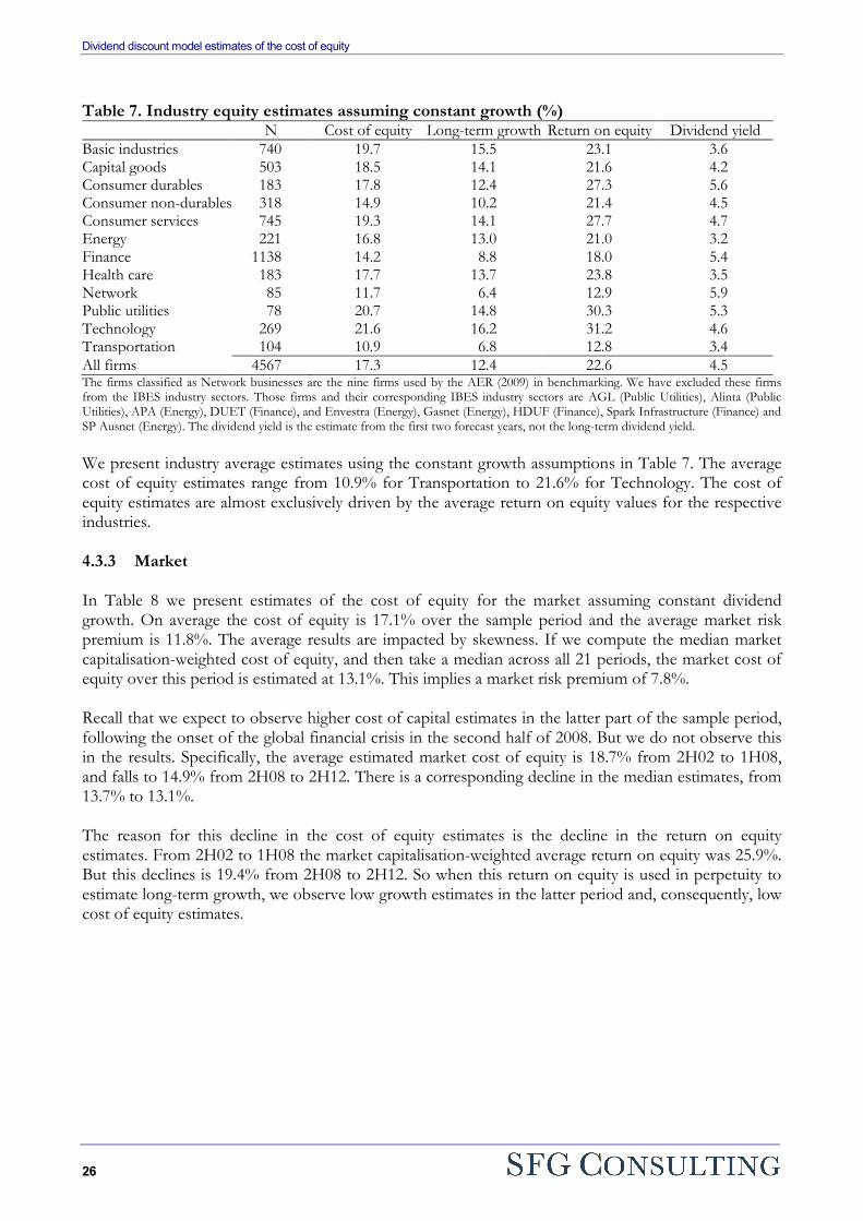
Dividend discount model estimates of the cost of equity
26
Table 7. Industry equity estimates assuming constant growth (%) N Cost of equity Long-term growth Return on equity Dividend yield Basic industries 740 19.7 15.5 23.1 3.6 Capital goods 503 18.5 14.1 21.6 4.2 Consumer durables 183 17.8 12.4 27.3 5.6 Consumer non-durables 318 14.9 10.2 21.4 4.5 Consumer services 745 19.3 14.1 27.7 4.7 Energy 221 16.8 13.0 21.0 3.2 Finance 1138 14.2 8.8 18.0 5.4 Health care 183 17.7 13.7 23.8 3.5 Network 85 11.7 6.4 12.9 5.9 Public utilities 78 20.7 14.8 30.3 5.3 Technology 269 21.6 16.2 31.2 4.6 Transportation 104 10.9 6.8 12.8 3.4 All firms 4567 17.3 12.4 22.6 4.5 The firms classified as Network businesses are the nine firms used by the AER (2009) in benchmarking. We have excluded these firms from the IBES industry sectors. Those firms and their corresponding IBES industry sectors are AGL (Public Utilities), Alinta (Public Utilities), APA (Energy), DUET (Finance), and Envestra (Energy), Gasnet (Energy), HDUF (Finance), Spark Infrastructure (Finance) and SP Ausnet (Energy). The dividend yield is the estimate from the first two forecast years, not the long-term dividend yield. We present industry average estimates using the constant growth assumptions in Table 7. The average cost of equity estimates range from 10.9% for Transportation to 21.6% for Technology. The cost of equity estimates are almost exclusively driven by the average return on equity values for the respective industries. 4.3.3 Market In Table 8 we present estimates of the cost of equity for the market assuming constant dividend growth. On average the cost of equity is 17.1% over the sample period and the average market risk premium is 11.8%. The average results are impacted by skewness. If we compute the median market capitalisation-weighted cost of equity, and then take a median across all 21 periods, the market cost of equity over this period is estimated at 13.1%. This implies a market risk premium of 7.8%. Recall that we expect to observe higher cost of capital estimates in the latter part of the sample period, following the onset of the global financial crisis in the second half of 2008. But we do not observe this in the results. Specifically, the average estimated market cost of equity is 18.7% from 2H02 to 1H08, and falls to 14.9% from 2H08 to 2H12. There is a corresponding decline in the median estimates, from 13.7% to 13.1%. The reason for this decline in the cost of equity estimates is the decline in the return on equity estimates. From 2H02 to 1H08 the market capitalisation-weighted average return on equity was 25.9%. But this declines is 19.4% from 2H08 to 2H12. So when this return on equity is used in perpetuity to estimate long-term growth, we observe low growth estimates in the latter period and, consequently, low cost of equity estimates.
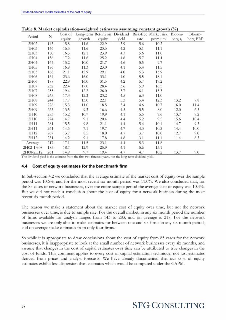
Dividend discount model estimates of the cost of equity
27
Table 8. Market capitalisation-weighted estimates assuming constant growth (%)
Period N Cost of equity
Long-term growth
Return on equity
Dividend yield
Risk-free rate
Market risk premium
Bloom-berg re
Bloom-berg ERP
2H02 143 15.8 11.6 22.9 3.9 5.6 10.2 1H03 146 16.3 11.6 23.3 4.2 5.1 11.1 2H03 150 16.5 12.1 23.9 4.3 5.6 11.0 1H04 156 17.2 11.6 25.2 4.6 5.7 11.4 2H04 164 15.2 10.0 21.7 4.6 5.5 9.7 1H05 186 16.8 11.3 23.0 4.1 5.4 11.5 2H05 168 21.1 12.9 29.1 4.0 5.3 15.9 1H06 164 23.6 16.0 33.1 4.0 5.5 18.1 2H06 188 22.9 16.0 31.5 4.2 5.7 17.2 1H07 232 22.4 17.0 28.4 3.6 5.9 16.5 2H07 253 19.4 12.2 26.0 3.7 6.1 13.3 1H08 265 17.3 12.3 23.2 4.5 6.3 11.0 2H08 244 17.7 13.0 22.1 5.3 5.4 12.3 13.2 7.8 1H09 228 15.3 11.0 18.5 5.4 4.6 10.7 16.0 11.4 2H09 263 13.5 9.3 16.6 4.5 5.5 8.0 12.0 6.5 1H10 283 15.2 10.7 19.9 4.1 5.5 9.6 13.7 8.2 2H10 274 14.7 9.1 20.4 4.4 5.2 9.5 15.6 10.4 1H11 281 15.5 9.8 21.1 4.4 5.4 10.1 14.7 9.3 2H11 261 14.5 7.1 19.7 4.7 4.3 10.2 14.4 10.0 1H12 267 13.7 8.5 18.0 4.7 3.7 10.0 12.7 9.0 2H12 251 14.2 9.1 17.8 4.8 3.1 11.1 11.4 8.3
Average 217 17.1 11.5 23.1 4.4 5.3 11.8 2H02-1H08 185 18.7 12.9 25.9 4.1 5.6 13.1 2H08-2H12 261 14.9 9.7 19.4 4.7 4.7 10.2 13.7 9.0
The dividend yield is the estimate from the first two forecast years, not the long-term dividend yield. 4.4 Cost of equity estimates for the benchmark firm In Sub-section 4.2 we concluded that the average estimate of the market cost of equity over the sample period was 10.6%, and for the most recent six month period was 11.0%. We also concluded that, for the 85 cases of network businesses, over the entire sample period the average cost of equity was 10.4%. But we did not reach a conclusion about the cost of equity for a network business during the most recent six month period. The reason we make a statement about the market cost of equity over time, but not the network businesses over time, is due to sample size. For the overall market, in any six month period the number of firms available for analysis ranges from 143 to 283, and on average is 217. For the network businesses we are only able to make estimates for between one and six firms in any six month period, and on average make estimates from only four firms. So while it is appropriate to draw conclusions about the cost of equity from 85 cases for the network businesses, it is inappropriate to look at the small number of network businesses every six months, and assume that changes in the cost of capital estimates over time can be attributed to true changes in the cost of funds. This comment applies to every cost of capital estimation technique, not just estimates derived from prices and analyst forecasts. We have already documented that our cost of equity estimates exhibit less dispersion than estimates which would be computed under the CAPM.
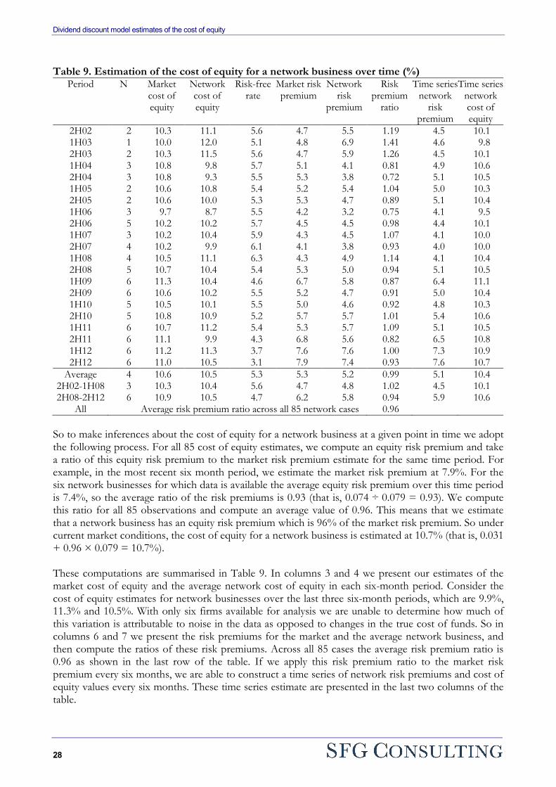
Dividend discount model estimates of the cost of equity
28
Table 9. Estimation of the cost of equity for a network business over time (%) Period N Market
cost of equity
Network cost of equity
Risk-free rate
Market risk premium
Network risk
premium
Risk premium
ratio
Time series network
risk premium
Time series network cost of equity
2H02 2 10.3 11.1 5.6 4.7 5.5 1.19 4.5 10.1 1H03 1 10.0 12.0 5.1 4.8 6.9 1.41 4.6 9.8 2H03 2 10.3 11.5 5.6 4.7 5.9 1.26 4.5 10.1 1H04 3 10.8 9.8 5.7 5.1 4.1 0.81 4.9 10.6 2H04 3 10.8 9.3 5.5 5.3 3.8 0.72 5.1 10.5 1H05 2 10.6 10.8 5.4 5.2 5.4 1.04 5.0 10.3 2H05 2 10.6 10.0 5.3 5.3 4.7 0.89 5.1 10.4 1H06 3 9.7 8.7 5.5 4.2 3.2 0.75 4.1 9.5 2H06 5 10.2 10.2 5.7 4.5 4.5 0.98 4.4 10.1 1H07 3 10.2 10.4 5.9 4.3 4.5 1.07 4.1 10.0 2H07 4 10.2 9.9 6.1 4.1 3.8 0.93 4.0 10.0 1H08 4 10.5 11.1 6.3 4.3 4.9 1.14 4.1 10.4 2H08 5 10.7 10.4 5.4 5.3 5.0 0.94 5.1 10.5 1H09 6 11.3 10.4 4.6 6.7 5.8 0.87 6.4 11.1 2H09 6 10.6 10.2 5.5 5.2 4.7 0.91 5.0 10.4 1H10 5 10.5 10.1 5.5 5.0 4.6 0.92 4.8 10.3 2H10 5 10.8 10.9 5.2 5.7 5.7 1.01 5.4 10.6 1H11 6 10.7 11.2 5.4 5.3 5.7 1.09 5.1 10.5 2H11 6 11.1 9.9 4.3 6.8 5.6 0.82 6.5 10.8 1H12 6 11.2 11.3 3.7 7.6 7.6 1.00 7.3 10.9 2H12 6 11.0 10.5 3.1 7.9 7.4 0.93 7.6 10.7
Average 4 10.6 10.5 5.3 5.3 5.2 0.99 5.1 10.4 2H02-1H08 3 10.3 10.4 5.6 4.7 4.8 1.02 4.5 10.1 2H08-2H12 6 10.9 10.5 4.7 6.2 5.8 0.94 5.9 10.6
All Average risk premium ratio across all 85 network cases 0.96 So to make inferences about the cost of equity for a network business at a given point in time we adopt the following process. For all 85 cost of equity estimates, we compute an equity risk premium and take a ratio of this equity risk premium to the market risk premium estimate for the same time period. For example, in the most recent six month period, we estimate the market risk premium at 7.9%. For the six network businesses for which data is available the average equity risk premium over this time period is 7.4%, so the average ratio of the risk premiums is 0.93 (that is, 0.074 ÷ 0.079 = 0.93). We compute this ratio for all 85 observations and compute an average value of 0.96. This means that we estimate that a network business has an equity risk premium which is 96% of the market risk premium. So under current market conditions, the cost of equity for a network business is estimated at 10.7% (that is, 0.031 + 0.96 × 0.079 = 10.7%). These computations are summarised in Table 9. In columns 3 and 4 we present our estimates of the market cost of equity and the average network cost of equity in each six-month period. Consider the cost of equity estimates for network businesses over the last three six-month periods, which are 9.9%, 11.3% and 10.5%. With only six firms available for analysis we are unable to determine how much of this variation is attributable to noise in the data as opposed to changes in the true cost of funds. So in columns 6 and 7 we present the risk premiums for the market and the average network business, and then compute the ratios of these risk premiums. Across all 85 cases the average risk premium ratio is 0.96 as shown in the last row of the table. If we apply this risk premium ratio to the market risk premium every six months, we are able to construct a time series of network risk premiums and cost of equity values every six months. These time series estimate are presented in the last two columns of the table.
Dividend discount model estimates of the cost of equity
29
5. Conclusion Over the 10.5 year period the estimated cost of equity for the average listed firm in the Australian market was 10.8%. The average estimate of the market cost of equity over this period is 10.6%, which represents a market risk premium over the entire sample period of 5.3%.25 For the nine listed energy network businesses previously used by the regulator in comparable firm analysis, the average estimated cost of equity is 10.4%. For the Australian market, the average cost of equity increases subsequent to the global financial crisis, which is consistent with expectations. These estimates represent equity investors’ required returns from dividends and capital gains only. If compensation for imputation credits or other tax benefits forms part of the regulated return, that regulated return must be higher than the figures presented here to account for those tax benefits. The estimated prevailing market cost of equity is 11.0% which represents a market risk premium of 7.9%. For the nine listed energy network businesses previously used by the regulator in comparable firm analysis, the estimated prevailing cost of equity is 10.7%. This is computed by adding 96% of the market risk premium to the risk-free rate, where the risk ratio of 0.96 is estimated with respect to all available data. In forming these estimates we incorporated an assumption that returns on investment, reinvestment rates and long-term growth rates revert to normal levels over time. But we do not impose values for these normal values. Rather, we select parameter inputs which set the present value of expected dividends equal to analyst price targets, and which allow for the smoothest transition to long-term growth. The resulting cost of capital estimates exhibit less dispersion than estimates which would result from the CAPM, if beta estimates are formed on the basis of regressions of historical stock returns on market returns. They exhibit less variation over time than would result from adding 6% to the risk-free rate of interest, which is the current practice of the regulator. They also increase during the period subsequent to the onset of the global financial crisis. We also compiled estimates of the cost of equity assuming constant growth, whereby returns on investment are projected to remain at the initial level in perpetuity. These estimates exhibit far greater dispersion than the estimates derived from the assumption that growth is mean-reverting. They are also higher, on average, because there is no constraint on investment returns. This results in the cost of equity estimates decreasing subsequent to the onset of the global financial crisis. This occurs because prior to the crisis, firms were reporting high returns on investment, and this flows through to high estimates for growth and therefore high estimates of the cost of equity. Subsequent to the crisis, returns on investment declined, leading to lower growth outcomes and therefore lower estimates of the cost of equity. The key point is that implementing a constant growth version of the dividend discount model for individual firms cannot feasibly be implemented using very recent data to estimate reinvestment rates and returns on equity. To implement a constant growth model therefore requires the analyst to impose a judgment on the “correct” growth rate, or at least exclude observations from this recent data in which the growth rate is unreasonably high or low to be a constant rate. But this basically means that the cost of equity is whatever the analyst decides it is – assume low growth rates and the cost of equity is low; assume high growth rates and the cost of equity is high. That is why it is crucial for the analyst to rely upon a systematic process for estimating growth, and not subjective judgment.
25 The difference between these two averages is that the value of 10.7% is the average cost of equity estimate from all observations in the sample, while the value of 10.5% is computed by taking a market capitalisation-weighted average every six months, and then taking an average of these six monthly averages.
Dividend discount model estimates of the cost of equity
30
The mean-reverting process used in this paper for estimation generates cost of capital estimates which are derived in an objective manner and generate outcomes consistent with actual market pricing. An alternative assumption sometimes invoked in dividend growth model analysis is that long-term investment returns equal the cost of capital. Under this assumption the long-term price/earnings ratio is the inverse of the cost of equity, which would imply price/earnings ratios well below what we actually observe for the largest, most mature firms. The long-term projected price/earnings ratios resulting from our analysis are closer to what we actually observe for this established firms.
Dividend discount model estimates of the cost of equity
31
6. References Australian Energy Regulator, 2009. “Electricity transmission and distribution network service
providers: Review of the weighted average cost of capital (WACC) parameters,” May 2009. Australian Energy Regulator, 2013. “Consultation paper: Rate of return guidelines,” May. Competition Economists Group, 2012a. “Internal consistency of risk-free rate and MRP in the
CAPM,” Report prepared for Envestra, SP AusNet, Multinet and APA, March. Competition Economists Group, 2012b. “Update to March 2012 Report: On Consistency of the Risk
Free Rate and MRP in the CAPM: Report prepared for Envestra, SP AusNet, Multinet and APA,” November.
Capital Research, 2013. “Forward estimate of the market risk premium: Update,” A report prepared for
the Victorian gas transmission and distribution businesses: APA Group, Envestra, Multinet Gas and SP AusNet, March 2012.
Cheng, Q., 2005. “What determines residual income?” Accounting Review, 80, 85–112. Easton, P., 2004. “PE ratios, PEG ratios, and estimating the implied expected rate of return on equity
capital,” The Accounting Review, 79, 73–96. Easton, P., 2006. “Use of forecasts of earnings to estimate and compare cost of capital across regimes,”
Journal of Business Finance and Accounting, 33, 374–394. Easton, P., G. Taylor, P. Shroff, and T. Sougiannis, 2004. “Using forecasts of earnings to
simultaneously estimate growth and the rate of return on equity investment,” Journal of Accounting Research, 40, 675–676.
Fitzgerald, T., S. Gray, J. Hall and R. Jeyaraj, 2013. “Unconstrained estimates of the equity risk
premium,” Review of Accounting Studies, 18, on-line release 8 May 2013. Lally, M., 2013. “The dividend growth model,” 4 March. Li, Y., D. Ng and B. Swaminathan, 2013. “Predicting market returns using aggregate implied cost of
capital,” Forthcoming Journal of Financial Economics. Lintner, J., 1965. “The valuation of risk assets and the selection of risky investments in stock portfolios
and capital budgets,” Review of Economics and Statistics, 47, 13–37. NERA Economic Consulting, 2012. “Prevailing conditions and the market risk premium,” A report for
APA Group, Envestra, Multinet & SP AusNet, March. Officer, R., 1994. “The cost of capital of a company under an imputation tax system,” Accounting and
Finance, 1, 1 – 36. O’Hanlon, J., and A. Steele, 2000. “Estimating the equity risk premium using accounting
fundamentals,” Journal of Business Finance and Accounting, 27, 1051–84. SFG Consulting, 2013. “Dividend discount model estimates of the cost of equity,” 13 June.
Dividend discount model estimates of the cost of equity
32
Sharpe, W., 1964. “Capital asset prices: A theory of market equilibrium under conditions of risk,” Journal of Finance, 19, 425–442.
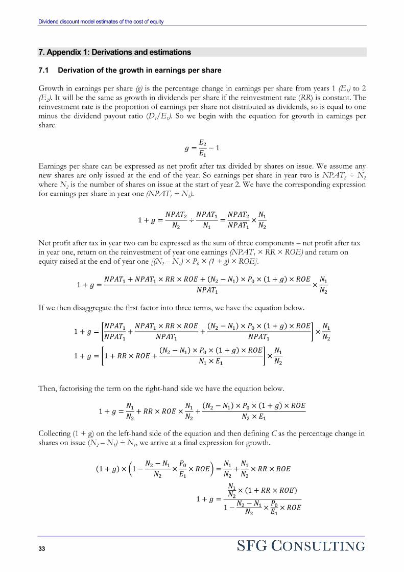
Dividend discount model estimates of the cost of equity
33
7. Appendix 1: Derivations and estimations 7.1 Derivation of the growth in earnings per share Growth in earnings per share (g) is the percentage change in earnings per share from years 1 (E1) to 2 (E2). It will be the same as growth in dividends per share if the reinvestment rate (RR) is constant. The reinvestment rate is the proportion of earnings per share not distributed as dividends, so is equal to one minus the dividend payout ratio (D1/E1). So we begin with the equation for growth in earnings per share.
𝑔 =𝐸2
𝐸1− 1
Earnings per share can be expressed as net profit after tax divided by shares on issue. We assume any new shares are only issued at the end of the year. So earnings per share in year two is NPAT2 ÷ N2 where N2 is the number of shares on issue at the start of year 2. We have the corresponding expression for earnings per share in year one (NPAT1 ÷ N1).
1 + 𝑔 =𝑁𝑃𝐴𝑇2
𝑁2÷
𝑁𝑃𝐴𝑇1
𝑁1=
𝑁𝑃𝐴𝑇2
𝑁𝑃𝐴𝑇1×
𝑁1
𝑁2
Net profit after tax in year two can be expressed as the sum of three components – net profit after tax in year one, return on the reinvestment of year one earnings (NPAT1 × RR × ROE) and return on equity raised at the end of year one [(N2 – N1) × P0 × (1 + g) × ROE].
1 + 𝑔 =𝑁𝑃𝐴𝑇1 + 𝑁𝑃𝐴𝑇1 × 𝑅𝑅 × 𝑅𝑂𝐸 + (𝑁2 − 𝑁1) × 𝑃0 × (1 + 𝑔) × 𝑅𝑂𝐸
𝑁𝑃𝐴𝑇1×
𝑁1
𝑁2
If we then disaggregate the first factor into three terms, we have the equation below.
1 + 𝑔 = �𝑁𝑃𝐴𝑇1
𝑁𝑃𝐴𝑇1+
𝑁𝑃𝐴𝑇1 × 𝑅𝑅 × 𝑅𝑂𝐸𝑁𝑃𝐴𝑇1
+(𝑁2 − 𝑁1) × 𝑃0 × (1 + 𝑔) × 𝑅𝑂𝐸
𝑁𝑃𝐴𝑇1� ×
𝑁1
𝑁2
1 + 𝑔 = �1 + 𝑅𝑅 × 𝑅𝑂𝐸 +(𝑁2 − 𝑁1) × 𝑃0 × (1 + 𝑔) × 𝑅𝑂𝐸
𝑁1 × 𝐸1� ×
𝑁1
𝑁2
Then, factorising the term on the right-hand side we have the equation below.
1 + 𝑔 =𝑁1
𝑁2+ 𝑅𝑅 × 𝑅𝑂𝐸 ×
𝑁1
𝑁2+
(𝑁2 − 𝑁1) × 𝑃0 × (1 + 𝑔) × 𝑅𝑂𝐸𝑁2 × 𝐸1
Collecting (1 + g) on the left-hand side of the equation and then defining C as the percentage change in shares on issue (N2 – N1) ÷ N1, we arrive at a final expression for growth.
(1 + 𝑔) × �1 −𝑁2 − 𝑁1
𝑁2×
𝑃0
𝐸1× 𝑅𝑂𝐸� =
𝑁1
𝑁2+
𝑁1
𝑁2× 𝑅𝑅 × 𝑅𝑂𝐸
1 + 𝑔 =
𝑁1𝑁2
× (1 + 𝑅𝑅 × 𝑅𝑂𝐸)
1 − 𝑁2 − 𝑁1𝑁2
× 𝑃0𝐸1
× 𝑅𝑂𝐸
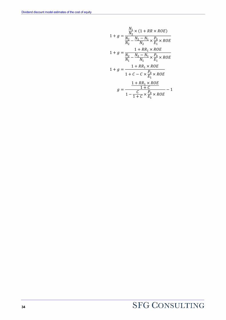
Dividend discount model estimates of the cost of equity
34
1 + 𝑔 =
𝑁1𝑁2
× (1 + 𝑅𝑅 × 𝑅𝑂𝐸)
𝑁2𝑁2
− 𝑁2 − 𝑁1𝑁2
× 𝑃0𝐸1
× 𝑅𝑂𝐸
1 + 𝑔 =1 + 𝑅𝑅1 × 𝑅𝑂𝐸
𝑁2𝑁1
− 𝑁2 − 𝑁1𝑁1
× 𝑃0𝐸1
× 𝑅𝑂𝐸
1 + 𝑔 =1 + 𝑅𝑅1 × 𝑅𝑂𝐸
1 + 𝐶 − 𝐶 × 𝑃0𝐸1
× 𝑅𝑂𝐸
𝑔 =1 + 𝑅𝑅1 × 𝑅𝑂𝐸
1 + 𝐶1 − 𝐶
1 + 𝐶 × 𝑃0𝐸1
× 𝑅𝑂𝐸− 1
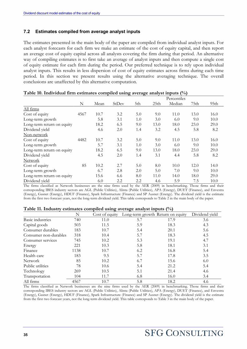
Dividend discount model estimates of the cost of equity
35
7.2 Estimates compiled from average analyst inputs The estimates presented in the main body of the paper are compiled from individual analyst inputs. For each analyst forecasts for each firm we make an estimate of the cost of equity capital, and then report an average cost of equity capital across all analysts covering the firm during that period. An alternative way of compiling estimates is to first take an average of analyst inputs and then compute a single cost of equity estimate for each firm during the period. Our preferred technique is to rely upon individual analyst inputs. This results in less dispersion of cost of equity estimates across firms during each time period. In this section we present results using the alternative averaging technique. The overall conclusions are unaffected by this alternative computation. Table 10. Individual firm estimates compiled using average analyst inputs (%)
Percentiles N Mean StDev 5th 25th Median 75th 95th
All firms Cost of equity 4567 10.7 3.2 5.0 9.0 11.0 13.0 16.0 Long-term growth 5.8 3.1 1.0 3.0 6.0 9.0 10.0 Long-term return on equity 18.2 6.5 9.0 13.0 18.0 23.0 29.0 Dividend yield 4.6 2.0 1.4 3.2 4.5 5.8 8.2 Non-network Cost of equity 4482 10.7 3.2 5.0 9.0 11.0 13.0 16.0 Long-term growth 5.7 3.1 1.0 3.0 6.0 9.0 10.0 Long-term return on equity 18.2 6.5 9.0 13.0 18.0 23.0 29.0 Dividend yield 4.5 2.0 1.4 3.1 4.4 5.8 8.2 Network Cost of equity 85 10.2 2.7 5.0 8.0 10.0 12.0 14.0 Long-term growth 6.7 2.8 2.0 5.0 7.0 9.0 10.0 Long-term return on equity 15.6 6.6 8.0 11.0 14.0 18.0 29.0 Dividend yield 6.0 2.2 2.2 4.6 5.9 7.5 10.0 The firms classified as Network businesses are the nine firms used by the AER (2009) in benchmarking. Those firms and their corresponding IBES industry sectors are AGL (Public Utilities), Alinta (Public Utilities), APA (Energy), DUET (Finance), and Envestra (Energy), Gasnet (Energy), HDUF (Finance), Spark Infrastructure (Finance) and SP Ausnet (Energy). The dividend yield is the estimate from the first two forecast years, not the long-term dividend yield. This table corresponds to Table 2 in the main body of the paper. Table 11. Industry estimates compiled using average analyst inputs (%) N Cost of equity Long-term growth Return on equity Dividend yield Basic industries 740 11.0 5.7 17.9 3.6 Capital goods 503 11.5 5.9 18.3 4.3 Consumer durables 183 10.7 5.4 20.1 5.6 Consumer non-durables 318 10.4 5.7 18.3 4.5 Consumer services 745 10.2 5.3 19.1 4.7 Energy 221 10.3 5.8 18.1 3.1 Finance 1138 10.7 6.2 16.8 5.4 Health care 183 9.5 5.7 17.8 3.5 Network 85 10.2 6.7 15.6 6.0 Public utilities 78 10.6 5.4 21.2 5.4 Technology 269 10.5 5.1 21.4 4.6 Transportation 104 11.7 6.8 16.0 3.4 All firms 4567 10.7 5.8 18.2 4.6 The firms classified as Network businesses are the nine firms used by the AER (2009) in benchmarking. Those firms and their corresponding IBES industry sectors are AGL (Public Utilities), Alinta (Public Utilities), APA (Energy), DUET (Finance), and Envestra (Energy), Gasnet (Energy), HDUF (Finance), Spark Infrastructure (Finance) and SP Ausnet (Energy). The dividend yield is the estimate from the first two forecast years, not the long-term dividend yield. This table corresponds to Table 3 in the main body of the paper.
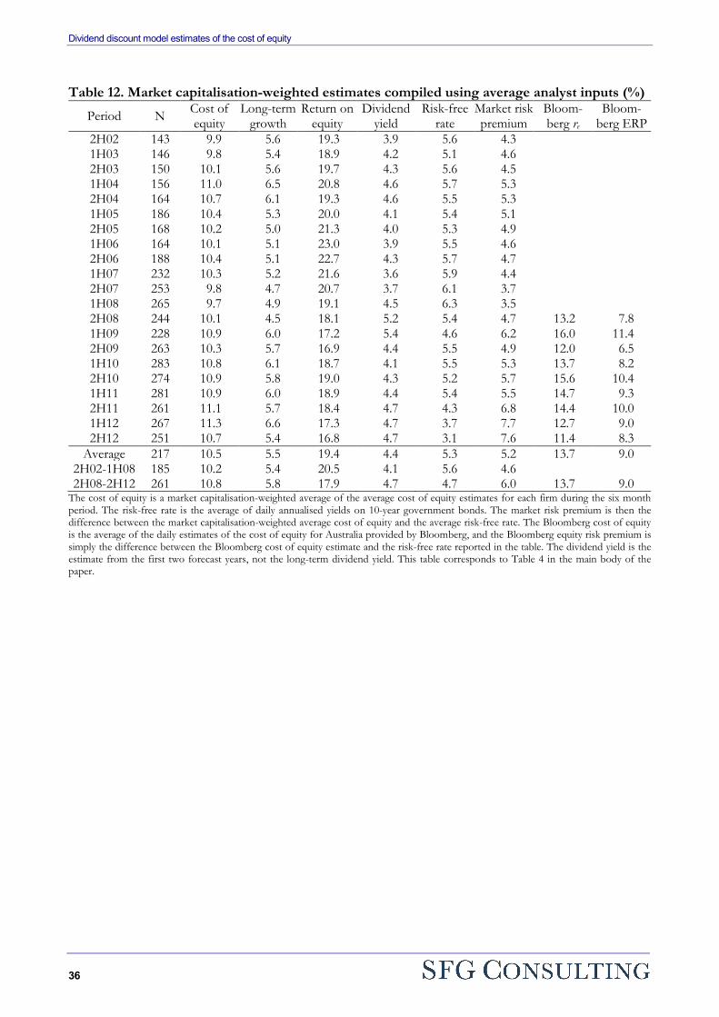
Dividend discount model estimates of the cost of equity
36
Table 12. Market capitalisation-weighted estimates compiled using average analyst inputs (%)
Period N Cost of equity
Long-term growth
Return on equity
Dividend yield
Risk-free rate
Market risk premium
Bloom-berg re
Bloom-berg ERP
2H02 143 9.9 5.6 19.3 3.9 5.6 4.3 1H03 146 9.8 5.4 18.9 4.2 5.1 4.6 2H03 150 10.1 5.6 19.7 4.3 5.6 4.5 1H04 156 11.0 6.5 20.8 4.6 5.7 5.3 2H04 164 10.7 6.1 19.3 4.6 5.5 5.3 1H05 186 10.4 5.3 20.0 4.1 5.4 5.1 2H05 168 10.2 5.0 21.3 4.0 5.3 4.9 1H06 164 10.1 5.1 23.0 3.9 5.5 4.6 2H06 188 10.4 5.1 22.7 4.3 5.7 4.7 1H07 232 10.3 5.2 21.6 3.6 5.9 4.4 2H07 253 9.8 4.7 20.7 3.7 6.1 3.7 1H08 265 9.7 4.9 19.1 4.5 6.3 3.5 2H08 244 10.1 4.5 18.1 5.2 5.4 4.7 13.2 7.8 1H09 228 10.9 6.0 17.2 5.4 4.6 6.2 16.0 11.4 2H09 263 10.3 5.7 16.9 4.4 5.5 4.9 12.0 6.5 1H10 283 10.8 6.1 18.7 4.1 5.5 5.3 13.7 8.2 2H10 274 10.9 5.8 19.0 4.3 5.2 5.7 15.6 10.4 1H11 281 10.9 6.0 18.9 4.4 5.4 5.5 14.7 9.3 2H11 261 11.1 5.7 18.4 4.7 4.3 6.8 14.4 10.0 1H12 267 11.3 6.6 17.3 4.7 3.7 7.7 12.7 9.0 2H12 251 10.7 5.4 16.8 4.7 3.1 7.6 11.4 8.3
Average 217 10.5 5.5 19.4 4.4 5.3 5.2 13.7 9.0 2H02-1H08 185 10.2 5.4 20.5 4.1 5.6 4.6 2H08-2H12 261 10.8 5.8 17.9 4.7 4.7 6.0 13.7 9.0
The cost of equity is a market capitalisation-weighted average of the average cost of equity estimates for each firm during the six month period. The risk-free rate is the average of daily annualised yields on 10-year government bonds. The market risk premium is then the difference between the market capitalisation-weighted average cost of equity and the average risk-free rate. The Bloomberg cost of equity is the average of the daily estimates of the cost of equity for Australia provided by Bloomberg, and the Bloomberg equity risk premium is simply the difference between the Bloomberg cost of equity estimate and the risk-free rate reported in the table. The dividend yield is the estimate from the first two forecast years, not the long-term dividend yield. This table corresponds to Table 4 in the main body of the paper.
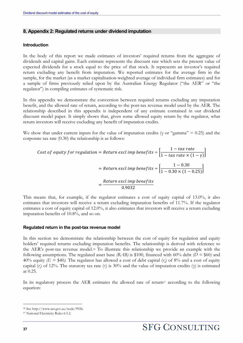
Dividend discount model estimates of the cost of equity
37
8. Appendix 2: Regulated returns under dividend imputation
Introduction In the body of this report we made estimates of investors’ required returns from the aggregate of dividends and capital gains. Each estimate represents the discount rate which sets the present value of expected dividends for a stock equal to the price of that stock. It represents an investor’s required return excluding any benefit from imputation. We reported estimates for the average firm in the sample, for the market (as a market capitalisation-weighted average of individual firm estimates) and for a sample of firms previously relied upon by the Australian Energy Regulator (“the AER” or “the regulator”) in compiling estimates of systematic risk. In this appendix we demonstrate the conversion between required returns excluding any imputation benefit, and the allowed rate of return, according to the post-tax revenue model used by the AER. The relationship described in this appendix is independent of any estimate contained in our dividend discount model paper. It simply shows that, given some allowed equity return by the regulator, what return investors will receive excluding any benefit of imputation credits. We show that under current inputs for the value of imputation credits (γ or “gamma” = 0.25) and the corporate tax rate (0.30) the relationship is as follows:
𝐶𝑜𝑠𝑡 𝑜𝑓 𝑒𝑞𝑢𝑖𝑡𝑦 𝑓𝑜𝑟 𝑟𝑒𝑔𝑢𝑙𝑎𝑡𝑖𝑜𝑛 = 𝑅𝑒𝑡𝑢𝑟𝑛 𝑒𝑥𝑐𝑙 𝑖𝑚𝑝 𝑏𝑒𝑛𝑒𝑓𝑖𝑡𝑠 ÷ �1 − 𝑡𝑎𝑥 𝑟𝑎𝑡𝑒
1 − 𝑡𝑎𝑥 𝑟𝑎𝑡𝑒 × (1 − 𝛾)�
= 𝑅𝑒𝑡𝑢𝑟𝑛 𝑒𝑥𝑐𝑙 𝑖𝑚𝑝 𝑏𝑒𝑛𝑒𝑓𝑖𝑡𝑠 ÷ �1 − 0.30
1 − 0.30 × (1 − 0.25)�
=𝑅𝑒𝑡𝑢𝑟𝑛 𝑒𝑥𝑐𝑙 𝑖𝑚𝑝 𝑏𝑒𝑛𝑒𝑓𝑖𝑡𝑠
0.9032
This means that, for example, if the regulator estimates a cost of equity capital of 13.0%, it also estimates that investors will receive a return excluding imputation benefits of 11.7%. If the regulator estimates a cost of equity capital of 12.0%, it also estimates that investors will receive a return excluding imputation benefits of 10.8%, and so on.
Regulated return in the post-tax revenue model In this section we demonstrate the relationship between the cost of equity for regulation and equity holders’ required returns excluding imputation benefits. The relationship is derived with reference to the AER’s post-tax revenue model.26 To illustrate this relationship we provide an example with the following assumptions. The regulated asset base (RAB) is $100, financed with 60% debt (D = $60) and 40% equity (E = $40). The regulator has allowed a cost of debt capital (rd) of 8% and a cost of equity capital (re) of 12%. The statutory tax rate (τ) is 30% and the value of imputation credits (γ) is estimated at 0.25. In its regulatory process the AER estimates the allowed rate of return27 according to the following equation:
26 See http://www.aer.gov.au/node/9926. 27 National Electricity Rules 6.5.2.
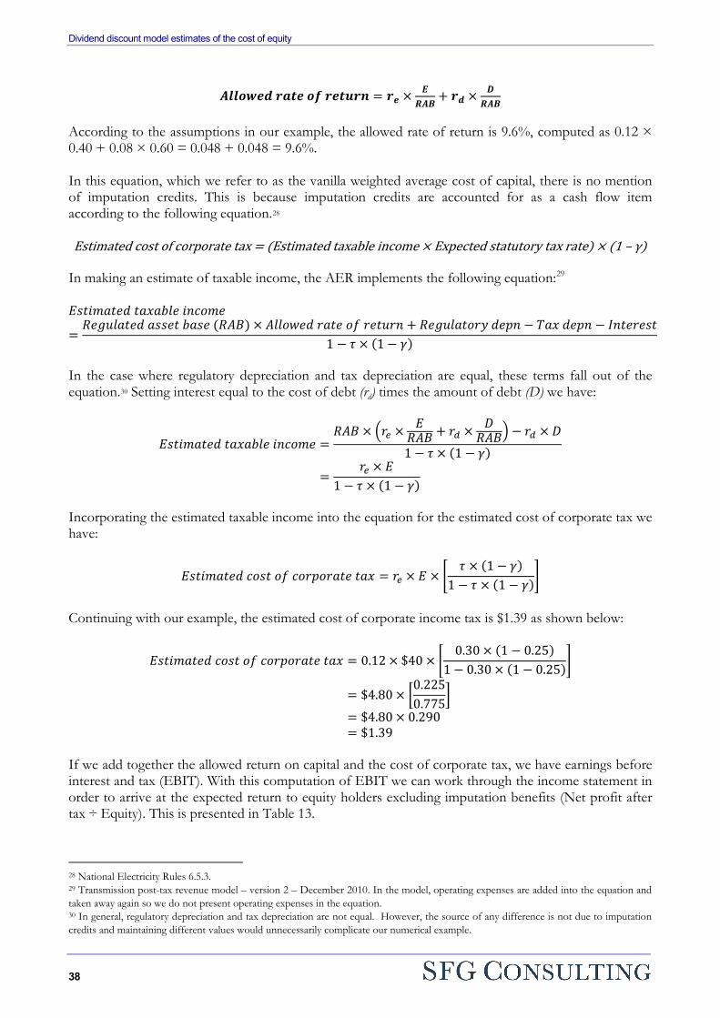
Dividend discount model estimates of the cost of equity
38
𝑨𝒍𝒍𝒐𝒘𝒆𝒅 𝒓𝒂𝒕𝒆 𝒐𝒇 𝒓𝒆𝒕𝒖𝒓𝒏 = 𝒓𝒆 × 𝑬𝑹𝑨𝑩
+ 𝒓𝒅 × 𝑫𝑹𝑨𝑩
According to the assumptions in our example, the allowed rate of return is 9.6%, computed as 0.12 × 0.40 + 0.08 × 0.60 = 0.048 + 0.048 = 9.6%. In this equation, which we refer to as the vanilla weighted average cost of capital, there is no mention of imputation credits. This is because imputation credits are accounted for as a cash flow item according to the following equation.28 Estimated cost of corporate tax = (Estimated taxable income × Expected statutory tax rate) × (1 – γ)
In making an estimate of taxable income, the AER implements the following equation:29 𝐸𝑠𝑡𝑖𝑚𝑎𝑡𝑒𝑑 𝑡𝑎𝑥𝑎𝑏𝑙𝑒 𝑖𝑛𝑐𝑜𝑚𝑒
=𝑅𝑒𝑔𝑢𝑙𝑎𝑡𝑒𝑑 𝑎𝑠𝑠𝑒𝑡 𝑏𝑎𝑠𝑒 (𝑅𝐴𝐵) × 𝐴𝑙𝑙𝑜𝑤𝑒𝑑 𝑟𝑎𝑡𝑒 𝑜𝑓 𝑟𝑒𝑡𝑢𝑟𝑛 + 𝑅𝑒𝑔𝑢𝑙𝑎𝑡𝑜𝑟𝑦 𝑑𝑒𝑝𝑛 − 𝑇𝑎𝑥 𝑑𝑒𝑝𝑛 − 𝐼𝑛𝑡𝑒𝑟𝑒𝑠𝑡
1 − 𝜏 × (1 − 𝛾)
In the case where regulatory depreciation and tax depreciation are equal, these terms fall out of the equation.30 Setting interest equal to the cost of debt (rd) times the amount of debt (D) we have:
𝐸𝑠𝑡𝑖𝑚𝑎𝑡𝑒𝑑 𝑡𝑎𝑥𝑎𝑏𝑙𝑒 𝑖𝑛𝑐𝑜𝑚𝑒 =𝑅𝐴𝐵 × �𝑟𝑒 × 𝐸
𝑅𝐴𝐵 + 𝑟𝑑 × 𝐷𝑅𝐴𝐵� − 𝑟𝑑 × 𝐷
1 − 𝜏 × (1 − 𝛾)
=𝑟𝑒 × 𝐸
1 − 𝜏 × (1 − 𝛾)
Incorporating the estimated taxable income into the equation for the estimated cost of corporate tax we have:
𝐸𝑠𝑡𝑖𝑚𝑎𝑡𝑒𝑑 𝑐𝑜𝑠𝑡 𝑜𝑓 𝑐𝑜𝑟𝑝𝑜𝑟𝑎𝑡𝑒 𝑡𝑎𝑥 = 𝑟𝑒 × 𝐸 × �𝜏 × (1 − 𝛾)
1 − 𝜏 × (1 − 𝛾)�
Continuing with our example, the estimated cost of corporate income tax is $1.39 as shown below:
𝐸𝑠𝑡𝑖𝑚𝑎𝑡𝑒𝑑 𝑐𝑜𝑠𝑡 𝑜𝑓 𝑐𝑜𝑟𝑝𝑜𝑟𝑎𝑡𝑒 𝑡𝑎𝑥 = 0.12 × $40 × �0.30 × (1 − 0.25)
1 − 0.30 × (1 − 0.25)�
= $4.80 × �0.2250.775�
= $4.80 × 0.290 = $1.39
If we add together the allowed return on capital and the cost of corporate tax, we have earnings before interest and tax (EBIT). With this computation of EBIT we can work through the income statement in order to arrive at the expected return to equity holders excluding imputation benefits (Net profit after tax ÷ Equity). This is presented in Table 13.
28 National Electricity Rules 6.5.3. 29 Transmission post-tax revenue model – version 2 – December 2010. In the model, operating expenses are added into the equation and taken away again so we do not present operating expenses in the equation. 30 In general, regulatory depreciation and tax depreciation are not equal. However, the source of any difference is not due to imputation credits and maintaining different values would unnecessarily complicate our numerical example.
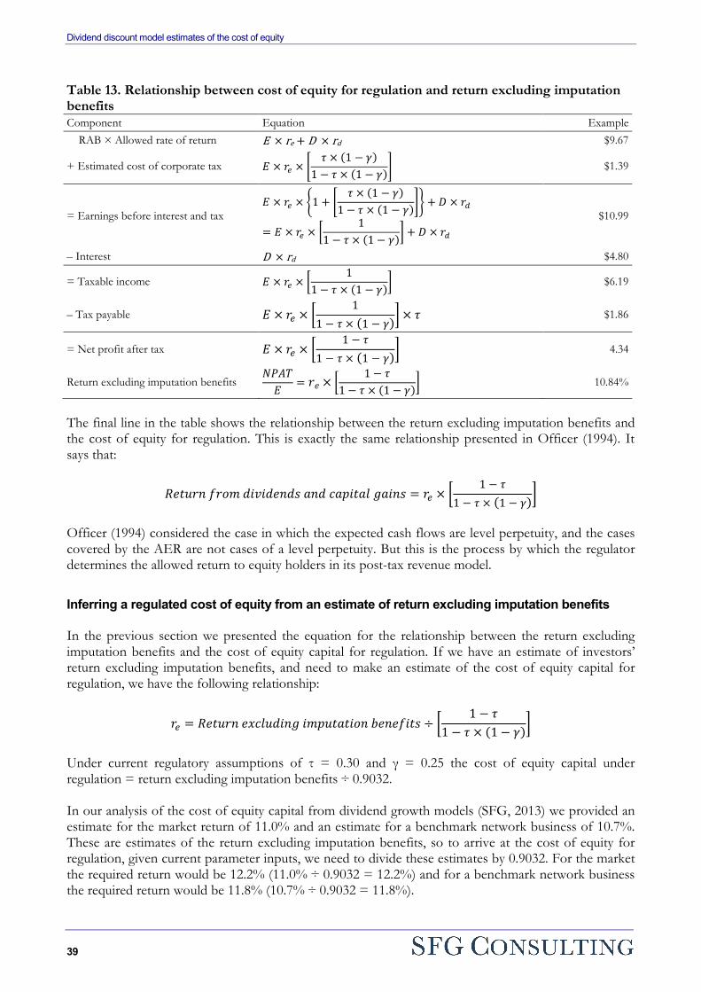
Dividend discount model estimates of the cost of equity
39
Table 13. Relationship between cost of equity for regulation and return excluding imputation benefits Component Equation Example RAB × Allowed rate of return E × re + D × rd $9.67
+ Estimated cost of corporate tax 𝐸 × 𝑟𝑒 × �𝜏 × (1 − 𝛾)
1 − 𝜏 × (1 − 𝛾)� $1.39
= Earnings before interest and tax 𝐸 × 𝑟𝑒 × �1 + �
𝜏 × (1 − 𝛾)1 − 𝜏 × (1 − 𝛾)�� + 𝐷 × 𝑟𝑑
= 𝐸 × 𝑟𝑒 × �1
1 − 𝜏 × (1 − 𝛾)� + 𝐷 × 𝑟𝑑 $10.99
– Interest D × rd $4.80
= Taxable income 𝐸 × 𝑟𝑒 × �1
1 − 𝜏 × (1 − 𝛾)� $6.19
– Tax payable 𝐸 × 𝑟𝑒 × �1
1 − 𝜏 × (1 − 𝛾)� × 𝜏 $1.86
= Net profit after tax 𝐸 × 𝑟𝑒 × �1 − 𝜏
1 − 𝜏 × (1 − 𝛾)� 4.34
Return excluding imputation benefits 𝑁𝑃𝐴𝑇
𝐸= 𝑟𝑒 × �
1 − 𝜏1 − 𝜏 × (1 − 𝛾)� 10.84%
The final line in the table shows the relationship between the return excluding imputation benefits and the cost of equity for regulation. This is exactly the same relationship presented in Officer (1994). It says that:
𝑅𝑒𝑡𝑢𝑟𝑛 𝑓𝑟𝑜𝑚 𝑑𝑖𝑣𝑖𝑑𝑒𝑛𝑑𝑠 𝑎𝑛𝑑 𝑐𝑎𝑝𝑖𝑡𝑎𝑙 𝑔𝑎𝑖𝑛𝑠 = 𝑟𝑒 × �1 − 𝜏
1 − 𝜏 × (1 − 𝛾)�
Officer (1994) considered the case in which the expected cash flows are level perpetuity, and the cases covered by the AER are not cases of a level perpetuity. But this is the process by which the regulator determines the allowed return to equity holders in its post-tax revenue model.
Inferring a regulated cost of equity from an estimate of return excluding imputation benefits In the previous section we presented the equation for the relationship between the return excluding imputation benefits and the cost of equity capital for regulation. If we have an estimate of investors’ return excluding imputation benefits, and need to make an estimate of the cost of equity capital for regulation, we have the following relationship:
𝑟𝑒 = 𝑅𝑒𝑡𝑢𝑟𝑛 𝑒𝑥𝑐𝑙𝑢𝑑𝑖𝑛𝑔 𝑖𝑚𝑝𝑢𝑡𝑎𝑡𝑖𝑜𝑛 𝑏𝑒𝑛𝑒𝑓𝑖𝑡𝑠 ÷ �1 − 𝜏
1 − 𝜏 × (1 − 𝛾)�
Under current regulatory assumptions of τ = 0.30 and γ = 0.25 the cost of equity capital under regulation = return excluding imputation benefits ÷ 0.9032. In our analysis of the cost of equity capital from dividend growth models (SFG, 2013) we provided an estimate for the market return of 11.0% and an estimate for a benchmark network business of 10.7%. These are estimates of the return excluding imputation benefits, so to arrive at the cost of equity for regulation, given current parameter inputs, we need to divide these estimates by 0.9032. For the market the required return would be 12.2% (11.0% ÷ 0.9032 = 12.2%) and for a benchmark network business the required return would be 11.8% (10.7% ÷ 0.9032 = 11.8%).
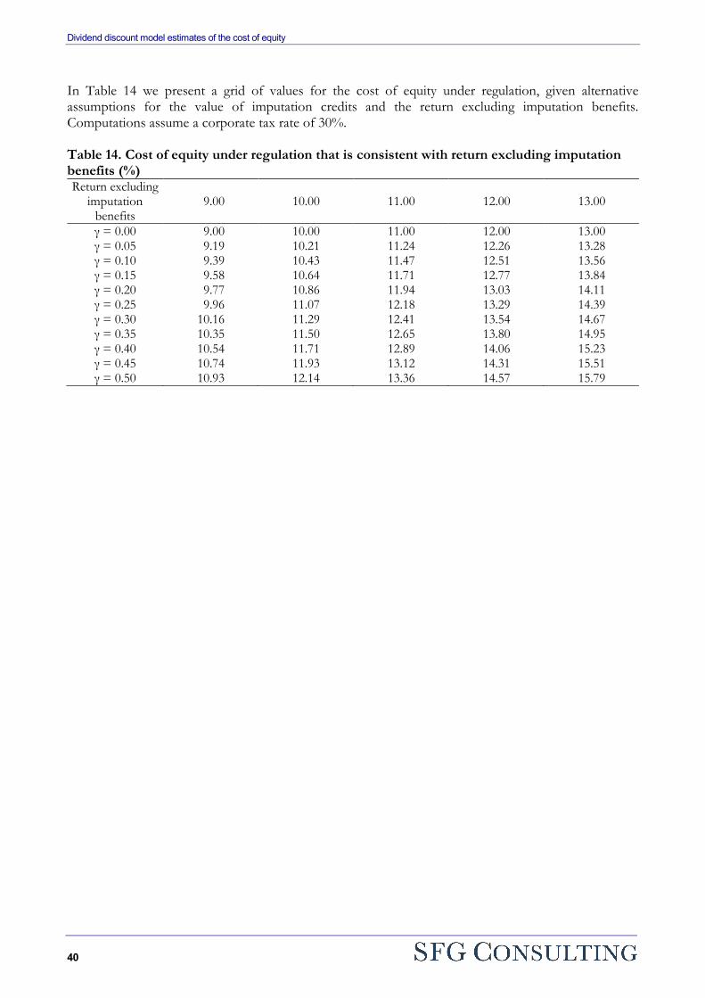
Dividend discount model estimates of the cost of equity
40
In Table 14 we present a grid of values for the cost of equity under regulation, given alternative assumptions for the value of imputation credits and the return excluding imputation benefits. Computations assume a corporate tax rate of 30%. Table 14. Cost of equity under regulation that is consistent with return excluding imputation benefits (%) Return excluding
imputation benefits
9.00 10.00 11.00 12.00 13.00
γ = 0.00 9.00 10.00 11.00 12.00 13.00 γ = 0.05 9.19 10.21 11.24 12.26 13.28 γ = 0.10 9.39 10.43 11.47 12.51 13.56 γ = 0.15 9.58 10.64 11.71 12.77 13.84 γ = 0.20 9.77 10.86 11.94 13.03 14.11 γ = 0.25 9.96 11.07 12.18 13.29 14.39 γ = 0.30 10.16 11.29 12.41 13.54 14.67 γ = 0.35 10.35 11.50 12.65 13.80 14.95 γ = 0.40 10.54 11.71 12.89 14.06 15.23 γ = 0.45 10.74 11.93 13.12 14.31 15.51 γ = 0.50 10.93 12.14 13.36 14.57 15.79
Dividend discount model estimates of the cost of equity
41
9. Terms of reference and qualifications This report was prepared by Professor Stephen Gray and Dr Jason Hall. Professor Gray and Dr Hall have made all they enquiries that they believe are desirable and appropriate and that no matters of significance that they regard as relevant have, to their knowledge, been withheld. Copies of the curriculum vitae of each author are attached as Attachment A to this report. Professor Gray and Dr Hall have been provided with a copy of the Federal Court of Australia’s “Guidelines for Expert Witnesses in Proceeding in the Federal Court of Australia.” The Report has been prepared in accordance with those Guidelines, which appear in the terms of reference, which appear in the terms of reference that are attached as Attachment B to this report.

Dividend discount model estimates of the cost of equity
42
Attachment A: CVs
1
Stephen F. Gray
University of Queensland Business School Brisbane 4072 AUSTRALIA
Office: +61-7-3346 8032 Email: [email protected]
Academic Qualifications 1995 Ph.D. (Finance), Graduate School of Business, Stanford University. Dissertation Title: Essays in Empirical Finance Committee Chairman: Ken Singleton 1989 LL.B. (Hons), Bachelor of Laws with Honours, University of Queensland. 1986 B.Com. (Hons), Bachelor of Commerce with Honours, University of Queensland. Employment History 2000-Present Professor of Finance, UQ Business School, University of Queensland. 1997-2000 Associate Professor of Finance, Department of Commerce, University of Queensland
and Research Associate Professor of Finance, Fuqua School of Business, Duke University.
1994-1997 Assistant Professor of Finance, Fuqua School of Business, Duke University. 1990-1993 Research Assistant, Graduate School of Business, Stanford University. 1988-1990 Assistant Professor of Finance, Department of Commerce, University of Queensland. 1987 Specialist Tutor in Finance, Queensland University of Technology. 1986 Teaching Assistant in Finance, Department of Commerce, University of Queensland. Academic Awards 2006 Outstanding Professor Award, Global Executive MBA, Fuqua School of Business, Duke
University. 2002 Journal of Financial Economics, All-Star Paper Award, for Modeling the Conditional
Distribution of Interest Rates as a Regime-Switching Process, JFE, 1996, 42, 27-62. 2002 Australian University Teaching Award – Business (a national award for all university
instructors in all disciplines). 2000 University of Queensland Award for Excellence in Teaching (a University-wide award). 1999 Outstanding Professor Award, Global Executive MBA, Fuqua School of Business, Duke
University. 1999 KPMG Teaching Prize, Department of Commerce, University of Queensland. 1998 Faculty Teaching Prize (Business, Economics, and Law), University of Queensland. 1991 Jaedicke Fellow in Finance, Doctoral Program, Graduate School of Business, Stanford University. 1989 Touche Ross Teaching Prize, Department of Commerce, University of Queensland. 1986 University Medal in Commerce, University of Queensland. Large Grants (over $100, 000) • Australian Research Council Linkage Grant, 2008—2010, Managing Asymmetry Risk ($320,000),
with T. Brailsford, J.Alcock, and Tactical Global Management. • Intelligent Grid Cluster, Distributed Energy – CSIRO Energy Transformed Flagship Collaboration
Cluster Grant, 2008-2010 ($552,000) • Australian Research Council Research Infrastructure Block Grant, 2007—2008, Australian
Financial Information Database ($279,754). • Australian Research Council Discovery Grant, 2006—2008, Capital Management in a Stochastic
Earnings Environment ($270,000). • Australian Research Council Discovery Grant, 2005—2007, Australian Cost of Equity. • Australian Research Council Discovery Grant, 2002—2004, Quantification Issues in Corporate
Valuation, the Cost of Capital, and Optimal Capital Structure.
2
• Australian Research Council Strategic Partnership Grant, 1997—2000, Electricity Contracts and Securities in a Deregulated Market: Valuation and Risk Management for Market Participants.
Current Research Interests Benchmark returns and the cost of capital. Corporate Finance. Capital structure. Real and strategic options and corporate valuation. Financial and credit risk management. Empirical finance and asset pricing. Publications
Faff, R., S. Gray and M. Poulsen, (2013), “Financial inflexibility and the value premium,” International Review of Finance, forthcoming.
Chen, E. T., S. Gray and J. Nowland, (2012), “Family representatives in family firms” Corporate Governance: An International Review, 21(3), 242-263.
Gray, S. and J. Hall, (2012), “Unconstrained estimates of the equity risk premium” Review of Accounting Studies, forthcoming.
Gray, S. and J. Nowland, (2012), “Is prior director experience valuable?” Accounting and Finance, forthcoming.
Chan, K-F., R. Brooks, S. Treepongkaruna and S. Gray, (2012), “Do Trading Hours Affect Volatility Links in the Foreign Exchange Market?” Australian Journal of Management, forthcoming.
Chen, E. T., S. Gray and J. Nowland, (2012), “Multiple founders and firm value” Pacific Basin Finance Journal, 20, 3, 398-415.
Chan, K-F., R. Brooks, S. Treepongkaruna and S. Gray, (2011), “Asset market linkages: Evidence from financial, commodity and real estate assets,” Journal of Banking and Finance, 35, 6, 1415-1426.
Parmenter, B, A. Breckenridge, and S. Gray, (2010), ‘Economic Analysis of the Government’s Recent Mining Tax Proposals’, Economic Papers: A Journal of Economics and Policy, 29(3), September, 279-91.
Gray, S., C. Gaunt and Y. Wu, (2010), “A comparison of alternative bankruptcy prediction models,” Journal of Contemporary Accounting and Economics, 6, 1, 34-45.
Feuerherdt, C., S. Gray and J. Hall, (2010), “The Value of Imputation Tax Credits on Australian Hybrid Securities,” International Review of Finance, 10, 3, 365-401.
Gray, S., J. Hall, D. Klease and A. McCrystal, (2009), “Bias, stability and predictive ability in the measurement of systematic risk,” Accounting Research Journal, 22, 3, 220-236.
Treepongkaruna, S. and S. Gray, (2009), “Information volatility links in the foreign exchange market,” Accounting and Finance, 49, 2, 385-405.
Costello, D., S. Gray, and A. McCrystal, (2008), “The diversification benefits of Australian equities,” JASSA, 2008, 4, 31-35.
Gray, S. and J. Hall, (2008), “The Relationship Between Franking Credits and the Market Risk Premium: A Reply,” Accounting and Finance, 48, 1, 133-142.
Gray, S., A. Mirkovic and V. Ragunathan, (2006), “The Determinants of Credit Ratings: Australian Evidence,” Australian Journal of Management, 31(2), 333-354.
Choy, E., S. Gray and V. Ragunathan, (2006), “The Effect of Credit Rating Changes on Australian Stock Returns,” Accounting and Finance, 46(5), 755-769.
Gray, S. and J. Hall, (2006), “The Relationship Between Franking Credits and the Market Risk Premium,” Accounting and Finance, 46(3), 405-428.
Gray, S. and S. Treepongkaruna, (2006), “Are there non-linearities in short-term interest rates?” Accounting and Finance, 46(1), 149-167.
Gray, P., S. Gray and T. Roche, (2005), “A Note on the Efficiency in Football Betting Markets: The Economic Significance of Trading Strategies,” Accounting and Finance, 45(2) 269-281.
3
Duffie, D., S. Gray and P. Hoang, (2004), “Volatility in Energy Prices. In V. Kaminski,” (Ed.), Managing Energy Price Risk: The New Challenges and Solutions (3rd ed.). London: Risk Books.
Cannavan, D., F. Finn and S. Gray, (2004), “The Value of Dividend Imputation Tax Credits in Australia,” Journal of Financial Economics, 73, 167-197.
Gray, S. and S. Treepongkaruna, (2003), “Valuing Interest Rate Derivatives Using a Monte-Carlo Approach,” Accounting and Finance, 43(2), 231-259.
Gray, S., T. Smith and R. Whaley, (2003), “Stock Splits: Implications for Investor Trading Costs,” Journal of Empirical Finance, 10, 271-303.
Gray, S. and S. Treepongkaruna, (2003), “On the Robustness of Short-term Interest Rate Models,” Accounting and Finance, 43(1), 87-121.
Gray, S. and S. Treepongkaruna, (2002), “How to Value Interest Rate Derivatives in a No-Arbitrage Setting,” Accounting Research Journal (15), 1.
Gray, P. and S. Gray, (2001), “A Framework for Valuing Derivative Securities,” Financial Markets Institutions & Instruments, 10(5), 253-276.
Gray, P. and S. Gray, (2001), “Option Pricing: A Synthesis of Alternate Approaches,” Accounting Research Journal, 14(1), 75-83.
Dahlquist, M. and S. Gray, (2000), “Regime-Switching and Interest Rates in the European Monetary System,” Journal of International Economics, 50(2), 399-419.
Bollen, N., S. Gray and R. Whaley, (2000), “Regime-Switching in Foreign Exchange Rates: Evidence from Currency Options,” Journal of Econometrics, 94, 239-276.
Duffie, D., S. Gray and P. Hoang, (1999), “Volatility in Energy Prices. In R. Jameson,” (Ed.), Managing Energy Price Risk (2nd ed.). London: Risk Publications.
Gray, S. and R. Whaley, (1999), “Reset Put Options: Valuation, Risk Characteristics, and an Example,” Australian Journal of Management, 24(1), 1-21.
Bekaert, G. and S. Gray, (1998), “Target Zones and Exchange Rates: An Empirical Investigation,” Journal of International Economics, 45(1), 1-35.
Gray, S. and R. Whaley, (1997), “Valuing S&P 500 Bear Market Warrants with a Periodic Reset,” Journal of Derivatives, 5(1), 99-106.
Gray, S. and P. Gray, (1997), “Testing Market Efficiency: Evidence from the NFL Sports Betting Market,” The Journal of Finance, 52(4), 1725-1737.
Gray, S. (1996), “Modeling the Conditional Distribution of Interest Rates as a Regime- Switching Process,” Journal of Financial Economics, 42, 27-62.
Gray, S. (1996), “Regime-Switching in Australian Interest Rates,” Accounting and Finance, 36(1), 65-88.
Brailsford, T., S. Easton, P.Gray and S. Gray, (1995), “The Efficiency of Australian Football Betting Markets,” Australian Journal of Management, 20(2), 167-196.
Duffie, D. and S. Gray, (1995), “Volatility in Energy Prices,” In R. Jameson (Ed.), Managing Energy Price Risk, London: Risk Publications.
Gray, S. and A. Lynch, (1990), “An Alternative Explanation of the January Anomaly,” Accounting Research Journal, 3(1), 19-27.
Gray, S. (1989), “Put Call Parity: An Extension of Boundary Conditions,” Australian Journal of Management, 14(2), 151-170.
Gray, S. (1988), “The Straddle and the Efficiency of the Australian Exchange Traded Options Market,” Accounting Research Journal, 1(2), 15-27.
Teaching Fuqua School of Business, Duke University, Student Evaluations (0-7 scale):
4
• Financial Management (MBA Core): Average 6.5 over 7 years. • Advanced Derivatives: Average 6.6 over 4 years. • Empirical Issues in Asset Pricing: Ph.D. Class
1999, 2006 Outstanding Professor Award, Global Executive MBA, Fuqua School of Business,
Duke University. UQ Business School, University of Queensland, Student Evaluations (0-7 scale):
• Finance (MBA Core): Average 6.6 over 10 years. • Corporate Finance Honours: Average 6.9 over 10 years.
2002 Australian University Teaching Award – Business (a national award for all university
instructors in all disciplines). 2000 University of Queensland Award for Excellence in Teaching. 1999 Department of Commerce KPMG Teaching Prize, University of Queensland. 1998 Faculty Teaching Prize, Faculty of Business Economics and Law, University of Queensland. 1998 Commendation for Excellence in Teaching, University-wide Teaching Awards, University of Queensland. 1989 Touche Ross Teaching Prize, Department of Commerce, University of Queensland. Board Positions 2002 - Present: Director, Financial Management Association of Australia Ltd. 2003 - Present: Director, Moreton Bay Boys College Ltd. (Chairman since 2007). 2002 - 2007: External Risk Advisor to Board of Enertrade (Queensland Power Trading Corporation
Ltd.) Consulting
Managing Director, Strategic Finance Group: www.sfgconsulting.com.au.
Consulting interests and specialties, with recent examples, include:
• Corporate finance ⇒ Listed multi-business corporation: Detailed financial modeling of each business unit,
analysis of corporate strategy, estimation of effects of alternate strategies, development of capital allocation framework.
• Capital management and optimal capital structure
⇒ State-owned electricity generator: Built detailed financial model to analyze effects of increased leverage on cost of capital, entity value, credit rating, and stability of dividends. Debt of $500 million issued.
• Cost of capital
⇒ Cost of Capital in the Public Sector: Provided advice to a government enterprise on how to estimate an appropriate cost of capital and benchmark return for Government-owned enterprises. Appearance as expert witness in legal proceedings that followed a regulatory determination.
⇒ Expert Witness: Produced a written report and provided court testimony on issues relating to the cost of capital of a cable TV business.
⇒ Regulatory Cost of Capital: Extensive work for regulators and regulated entities on all matters relating to estimation of weighted-average cost of capital.
• Valuation
⇒ Expert Witness: Produced a written report and provided court testimony. The issue was whether, during a takeover offer, the shares of the bidding firm were affected by a liquidity premium due to its incorporation in the major stock market index.
⇒ Expert Witness: Produced a written report and provided court testimony in relation to valuation issues involving an integrated mine and refinery.
5
• Capital Raising ⇒ Produced comprehensive valuation models in the context of capital raisings for a range of
businesses in a range of industries including manufacturing, film production, and biotechnology.
• Asset pricing and empirical finance
⇒ Expert Witness: Produced a written report on whether the client’s arbitrage-driven trading strategy caused undue movements in the prices of certain shares.
• Application of econometric techniques to applied problems in finance
⇒ Debt Structure Review: Provided advice to a large City Council on restructuring their debt portfolio. The issues involved optimisation of a range of performance measures for each business unit in the Council while simultaneously minimizing the volatility of the Council’s equity in each business unit.
⇒ Superannuation Fund Performance Benchmarking: Conducted an analysis of the techniques used by a large superannuation fund to benchmark its performance against competing funds.
• Valuation of derivative securities
⇒ Stochastic Volatility Models in Interest Rate Futures Markets: Estimated and implemented a number of models designed to predict volatility in interest rate futures markets.
• Application of option-pricing techniques to real project evaluation
⇒ Real Option Valuation: Developed a framework for valuing an option on a large office building. Acted as arbitrator between the various parties involved and reached a consensus valuation.
⇒ Real Option Valuation: Used real options framework in the valuation of a bio-tech company in the context of an M&A transaction.
17 June 2013
Jason Hall, PhD BCom(Hons) CFA Director SFG Consulting Level 1, South Bank House, Stanley Street Plaza South Bank, Queensland, Australia 4101 Phone: 61-7-3844 0684 Australia mobile: +61 419 120 348 [email protected]
Experience 2000-12 University of Queensland Business School, The University of Queensland (Senior Lecturer) 2008 Ross School of Business, The University of Michigan (Visiting Assistant Professor in Finance) 1997-99 Credit Suisse First Boston (Equities analyst) Education 2005 PhD in finance from The University of Queensland 2003 Chartered Financial Analyst designation by the CFA Institute 1996 Bachelor of Commerce with First Class Honours from The University of Queensland Research Journal articles Impact of sector versus security choice on equity portfolios, with Ben McVicar, Applied Financial Economics, 2013,
23 (12), 991 – 1004. Unconstrained estimates of the equity risk premium, with Stephen Gray, Tristan Fitzgerald and Ravi Jeyaraj, Review
of Accounting Studies, 2013, 18 (2), 560 – 639. Market risk exposure of merger arbitrage in Australia, with Matthew Pinnuck and Matthew Thorne, Accounting and
Finance, 2013, 53 (1), 185 – 215. The value of imputation credits on hybrid securities, with Clinton Feuerherdt and Stephen Gray, International Review
of Finance, 2010, 10 (3), 365 – 401. Forecast accuracy and stock recommendations, with Paul Tacon, Journal of Contemporary Accounting and
Economics, 2010, 6 (1), 18 – 33. Speculation and e-commerce: The long and the short of IT, with Colin Ferguson, Matthew Pinnuck and Frank Finn,
International Journal of Accounting Information Systems, 2010, 11 (2), 79 – 104. Bias, stability and predictive ability in the measurement of systematic risk, with Stephen Gray, Drew Klease and Alan
McCrystal, Accounting Research Journal, 2009, 22 (3), 220 – 236. Leveraged superannuation, with Peter Dunn and Scott Francis, Accounting and Finance, 2009, 49 (3), 505 – 529. Persistence in growth versus market expectations, with Matthew Tochterman, Australian Journal of Management,
2008, 33 (1), 169 – 199. Relationship between franking credits and the market risk premium: A reply, with Stephen Gray, Accounting and
Finance, 2008, 48 (1), 133 – 142. Comment on ‘Regulation and the term of the risk free rate: Implications of corporate debt’, Accounting Research
Journal, 2007, 20 (2), 81 – 86. Valuation of mining projects using option pricing techniques, with Shannon Nicholls, JASSA, 2007, Issue 4 (Summer),
22 – 29. Relationship between franking credits and the market risk premium, with Stephen Gray, Accounting and Finance,
2006, 46 (3), 405 – 428. Electronic commerce investments, the resource-based view of the firm, and firm market value, with Colin Ferguson
and Frank Finn, International Journal of Accounting Information Systems, 2005, 6 (1), 5 – 29. Auditor conservatism and voluntary disclosure: Evidence from the Year 2000 systems issue, with Peter Clarkson and
Colin Ferguson, Accounting and Finance, 2003, 43 (1), 21 – 40. Working papers The impact of security analyst recommendations on the trading of mutual funds, with David Costello, AFAANZ
Conference 2010 (Winner Best Paper in Finance), Australasian Finance and Banking Conference 2010, undergoing revisions for re-submission to Journal of Contemporary Accounting and Economics.
Portfolio rebalancing and mutual fund tournament behavior, with Paul Tacon, Finance and Corporate Governance Conference 2011, FIRN Frontiers in Finance Conference 2011, Financial Management Association Annual Meeting 2012, undergoing revisions for re-submission to Financial Management.
Resume of Jason Hall as at 17 June 2013
2
Forecasting stock returns using investor flows under short-sales constraints, with Paul Tacon, Australasian Finance and Banking Conference 2011, Finance and Corporate Governance Conference 2012, AFAANZ Conference 2012, Financial Management Association Annual Meeting 2012, Southern Finance Association Annual Meeting 2012.
Presentations Accounting and Finance Association of Australia and New Zealand Conference (5) 2005, 2007, 2009-10, 2012 Asian Finance Association Conference 2009 Australasian Finance and Banking Conference (2) 2008, 2010 Australian National University Seminar Series 2012 Coal Trade, hosted by AIC Worldwide 1999 Coaltrans Asia, hosted by Coaltrans Conference Limited 1999 Contemporary Accounting Research/Journal of Contemporary Accounting and Economics Joint Symposium 2009 CPA Mining and Energy Conference 2006 Financial Management Association 2012 First Annual Private Equity Conference, hosted by Television Education Network 2007 JBWere Family Business Conference 2010 Melbourne Centre for Consumer Finance Investment & Regulatory Symposium 2008 PhD Conference in Economics and Business, hosted by University of Western Australia 2003 Southern Finance Association 2012 University of Melbourne Seminar Series (2) 2005, 2010 University of Queensland Seminar Series 2008 Referee activity Accounting and Finance (8 reviews) 2003, 2005, 2009-13 Accounting Research Journal (3 reviews) 2002, 2006, 2010 Applied Financial Economics (3 reviews) 2012-13 Australian Journal of Management 2012 Contemporary Economic Policy 2011 Financial Review 2013 International Journal of Emerging Markets 2013 International Review of Finance 2012 MIS Quarterly 2003 Quarterly Journal of Finance and Accounting 2010 Quarterly Review of Economics and Finance 2012 Research grants PricewaterhouseCoopers/Accounting and Finance Association of Australia and New Zealand 2006: Returns, tax and
volatility – Superannuation choice with a complete information set ($8,500) Australian Research Council Discovery Grant 2002-4: Quantification issues in corporate valuation, the cost of capital
and optimal capital structure ($126,000) UQ New Staff Research Start-up Fund: The competitive advantage of investments in electronic commerce ($10,000) Research students PhD (1 student) 2012 – Paul Tacon Honours (20 students) 2012 – Edward Parslow (Carnegie Wylie) 2011 – James Lamb (Port Jackson Partners) 2010 – Jeremy Evans (JP Morgan), Sarah Thorne (JP Morgan), Alexandra Dwyer (Reserve Bank of Australia) 2009 – Tristan Fitzgerald (UNSW), David Costello (National Australia Bank), William Toe (Ernst & Young) 2008 – Ben McVicar (Credit Suisse), Matthew Thorne (Credit Suisse) 2007 – Sam Turner (ABN Amro Morgans) 2006 – Paul Tacon (PhD, UQ), Ravi Jeyaraj (Navis Capital), Thomas Green (Crescent Capital), Alexander Pascal-
Bossy (Macquarie) 2005 – Angela Gill (Wilson HTM), Andrew Wagner (Macquarie) 2004 – Matthew Tochterman (M. Fin. Eng., UC Berkeley), Justyna Lewandowska (JP Morgan), An Pham (UBS) Masters (2 students) 2003 – Scott Francis (A Clear Direction Financial Planning), Hernando Barrero (PricewaterhouseCoopers) PhD reader Damien Cannavan 2012
Resume of Jason Hall as at 17 June 2013
3
Teaching UQ Business School, The University of Queensland (Mean teacher ratings out of a possible 5.0) Awarded undergraduate teaching prize 2009 Empirical Finance Honours (2009-12; PhD and Honours students; avg. rating 4.1) Corporate Finance Honours (2005 & 2011; PhD and Honours students; avg. rating 4.7) Investments & Portfolio Management (2002-7, 2009-10 & 2012; B.Com, MBA & M.Com students; avg. rating 3.8) Corporate Finance (2002-4, 2006-10 & 2012; B.Com, MBA and M.Com students; avg. rating 3.8) Finance (2005-6; M.Com students; avg. rating 3.7) Corporate Finance and Investments (Mt Eliza Business School, Beijing 2003; MBA students) Technology Valuation and Project Evaluation (Singapore 2004; Masters of Technology Management students) Auditing (Summer 2000/1-2001/2; B.Com, MBA and M.Com students; avg. rating 3.8) Ross School of Business, The University of Michigan Corporate Financial Policy (2008; MBA students; avg. rating 4.3) Executive education Risk Management and Financial Analysis (Rabobank 2000-10) Financial Analysis of Innovative Investments (UQ Business School 2007) Credit Analysis (Queensland Treasury Corporation 2005) Capital Management (UQ Business School 2004) Making Critical Financial Decisions (UQ Business School 2003) Business Valuation and Analysis (UQ Business School 2003) Cost of Capital Estimation (UQ Business School 2003) Analysis of Real Options (Queensland Treasury 2003) Student competitions Rotman International Trading Competition Manager of the UQ Business School trading team (2007 & 2009-12) which competes annually at the University of Toronto amongst 50 teams. UQ is the 9th most successful entrant from 66 schools which have competed in any of the same years, finishing 3rd in 2010, 6th in 2007, 11th in 2009, 14th in 2011 and 18th in 2012. UBS Investment Banking Competition Judge for the UQ section 2006-7 & 2009-12. Faculty representative at the national section 2008. JP Morgan Deal Competition Judge for the UQ section 2007-8. Wilson HTM Research Report Competition Delivered two workshops as part of the 2006 competition and was one of three judges. Industry engagement From 2000-12, I have provided consulting services as part of SFG Consulting and UQBS Commercial. Services have been provided in conjunction with Frontier Economics, ARENA Consulting, Parsons Brinckerhoff and Uniquest. Retail electricity and gas margins in NSW (Independent Pricing and Regulatory Tribunal 2012) In 2006-7 and 2009-10 I acted as part of a team which was engaged to estimate electricity costs and margins for electricity and gas retailers in NSW. We have been reappointed for 2012-13. My role related to the estimation of a profit margin which would allow the retailer to earn a return commensurate its systematic risk. The approach developed was novel in that the margin was derived without reference to any pre-defined estimate of the asset base. Rather, the margin was a function of the potential increases or decreases in cash flows which would result from changes in economic conditions. Reports are available from IPART. Advice on rules to determine regulated rates of return (Australian Energy Markets Commission 2012) The AEMC is considering changes to the rules relating to regulation of electricity and gas networks. Independent rule change proposals have been put forward by the Australian Energy Regulator and the Energy Users Association of Australia. Both groups argue that application of the existing rules by the regulator generate upwardly-biased estimates of the regulated rate of return. As part of a team I am currently providing advice to the commission on whether the rule change proposals provide evidence on an upward bias, and if so, whether the proposed amendments are likely to reduce the extent of any bias. Expert evidence relating to regulated rates of return (Electricity network businesses 2011) In April 2011 the Australian Competition Tribunal heard an appeal by electricity networks on the regulated rate of return set by the Australian Energy Regulator. The issue was the value of dividend imputation tax credits. The Tribunal directed us to perform a dividend drop-off study to estimate the value of a distributed credit. Largely on the basis of our evidence the Tribunal determined that an appropriate value for a distributed credit was 35 per cent of face value. The Tribunal determination is available on its website and our expert report is available on request.
Resume of Jason Hall as at 17 June 2013
4
Estimation of risks associated with long-term generation contracts (New South Wales Treasury 2010) In 2010 the NSW Government privatised a segment of its electricity industry, by selling three electricity retailers and entering into two generation agreements termed GenTrader contracts. The state-owned generators agreed to provide generation capacity in exchange for a charge. The generators also agreed to pay penalties in the event that their availability was less than agreed. As part of a team, I provided advice to NSW Treasury on the risks associated with the contracts. The estimated penalties resulting from this analysis are used by NSW Treasury in their budgeting role and in providing forward-looking analysis to the Government. Litigation support relating to asset valuation (Alcan 2006-7) In 2006-7 I acted as part of a team which provided litigation support to Alcan in a dispute with the taxation authority in the Northern Territory. The dispute related to whether Alcan was required to pay stamp duty as a result of its acquisition of an additional 30 per cent interest in Gove Alumina Limited. One issue was whether the acquisition was land-rich, meaning that the proportion of the asset considered to be land exceeded a threshold triggering stamp duty. Methodology for evaluating public-private partnerships (Queensland Treasury Corporation 2005) In 2005 I acted as part of a team which advised QTC on evaluating public-private partnerships, which typically require subsidies to appeal to the private sector. We rebutted the conventional wisdom, adopted in NSW and Victoria, that the standard valuation approach is flawed for negative-NPV projects. Furthermore, we developed a technique to incorporate systematic risk directly into expected cash flows, which are then discounted at the risk-free rate. Litigation support Insolvency proceedings relating to the collapse of Octaviar (Public Trustee of Queensland 2008-9) Valuation of resource assets (Compass Resources 2007-8, Westpac Banking Corporation 2007) Appeals against regulatory determinations (Envestra 2007-8, Telstra 2008) Advice on whether loan repayments correspond to contract terms (Qld Dept. of Fair Trading 2005) Advice on whether port and channel assets were contributed and hence not part of regulated assets (Comalco 2004-5) Valuation Management performance securities (Collins Foods Group 2006-11, GroundProbe 2008-9) Ordinary shares in the context of an equity raising (Auscript 2007-8) Intangible assets (Inbartec 2007) Resources assets (Senex Energy 2012, Chalco 2007, Bank of Queensland 2007) Cost of capital estimation, advice and regulatory submissions Transport (Qantas 2008, QR National 2005 & 2012) Water (Essential Services Commission of South Australia 2012, ActewAGL 2012, IPART 2011, Metropolitan utilities
in Victoria 2004 & 2006-7, QCA 2002-3) Energy networks (Economic Regulation Authority in Western Australia 2009, Hong Kong Electric 2007, Envestra
2006-7 & 2012, Powercor 2005, AGL 2004, Energex 2003-4, Ergon Energy 2003-4) Local government networks (Queensland Competition Authority 2009) Electricity generation (National Generators Forum 2008) Environmental consulting (Ecowise 2007) Listed vs unlisted infrastructure funds across alternative European equity markets (ABN AMRO Rothschild 2007) Forestry assets (Queensland Department of Natural Resources 2004) Portfolio performance measurement Performance evaluation and benchmark derivation (Friday Investments 2010-12, Zupp Property Group 2011-12) Corporate finance Economic impact assessment of a proposed development of a retail shopping complex (Lend Lease 2006) Impact of an acquisition on dividend growth, earnings per share and share price (AGL 2003-4) Estimation of the optimal capital structure for electricity generation and distribution (NSW Treasury 2001-2) Review of the debt valuation model used by the Snowy Hydroelectric Authority (NSW Treasury 2002) Estimation of the optimal contract terms for coal sales to an electricity generator (NSW Treasury 2001-2) Econometrics Scoping study into the determinants of changes in tax debt in Australia (Australian Taxation Office 2007) Interests I am interested in sport as a participant and spectator. I finished 3rd on three occasions in the Brisbane Half Marathon (2005 & 2009-10), 8th in the Toronto Half Marathon (2002) and 3rd in the Australian Universities Marathon Championships (2003). I have finished 17 marathons, recording a best time of 2:47:54 in the Chicago Marathon 2011. From 1994-96 I was a member of The University of Queensland tennis team, which placed 1st at the Australian University Games in 1994.

Dividend discount model estimates of the cost of equity
43
Attachment B: Terms of reference
TERMS OF REFERENCE – DIVIDEND GROWTH MODEL
Background
The Australian Energy Regulator (AER) is developing a rate of return guideline that will form the basis of the regulated rate of return applied in energy network decisions. The AER published an issues paper in late December 2012 and a formal consultation paper in early May 2013 under the recently revised National Electricity Rules (NER) and National Gas Rules (NGR).
Under the previous NER, the AER was required to estimate the cost of equity for electricity network businesses using the Sharpe-Lintner version of the capital asset pricing model (CAPM). Although the previous NGR did not mandate the use of the Sharpe-Lintner CAPM, in practice, the AER also applied this approach in gas network decisions. The recently revised NER and NGR now require the AER to have regard to multiple financial models, Clause 6.5.2 of the rules states:1
“(e) In determining the allowed rate of return, regard must be had to:
(1) relevant estimation methods, financial models, market data and other evidence;(2) the desirability of using an approach that leads to the consistent application of any estimates of financial parameters that are relevant to the estimates of, and that are common to, the return on equity and the return on debt; and(3) any interrelationships between estimates of financial parameters that are relevant to the estimates of the return on equity and the return on debt.
…
Return on equity
(f) The return on equity for a regulatory control period must be estimated such that it contributes to the achievement of the allowed rate of return objective.
(g) In estimating the return on equity under paragraph (f), regard must be had to the prevailing conditions in the market for equity funds.”
These clauses require the AER to consider all relevant financial models and therefore provide greater scope to look at cost of equity models beyond the traditionally adopted Sharpe-Lintner CAPM.
As further detailed below, the Energy Network Association (ENA) would like to engage you to provide your opinion on cost of equity estimates using models other than the Sharpe-Lintner CAPM and, in particular, provide cost of equity estimates using the Fama-French three factor model, the dividend growth model (DGM) and the Black CAPM, within the scope of the allowed rate of return objective:2
“[t]he rate of return for a [Service Provider] is to be commensurate with the efficient financing costs of a benchmark efficient entity with a similar degree of risk as that which applies to the [Service Provider] in respect of the provision of [services].”
1 Rule 87 in the NGR contains identical provisions to clauses 6.5.2 and 6A.6.2 in the NER. 2 NER 6.5.2(c), 6A.6.2(c) and NGR 87 (3).
Scope of work
The ENA requests your opinion on estimating the cost of equity for a benchmark regulated Australian energy utility using the DGM that is consistent with the NER and NGR for energy regulatory purposes. Your analysis and findings should:
• Consider different versions of the DGM that maybe relevant to Australia, including both the Gordon growth model (GGM) and the DGM used by the Federal Energy Regulatory Commission (FERC) and other regulators in the US;
• Use robust methods and data to estimate input parameters , recognising: − any interrelationship between parameters, such as between share prices and expected
dividend growth; − any differences between the return on invested earnings and the cost of capital; and − any differences in applying the DGM to listed and unlisted firms;
• Estimate the cost of equity for both the average firm in Australia3 and the benchmark regulated energy utility;
• Consider any comments raised by the AER and other regulators about the applicability and reliability of the DGM in Australia, including the sensitivity of cost of equity estimates to the growth rate assumption;
• Provide a method for grossing up stock returns for the value of imputation credits; • Ensure, where relevant, consistency with other estimates of the cost of equity developed
using other models by the ENA, such as the Fama-French three factor model, the Sharpe-Lintner CAPM and the Black CAPM; and
• Detail the bases for the growth and dividend yield assumptions used to estimate the cost of equity should be well documented and justified. 4
In your opinion, do you agree that the below formulae is commonly referred to as the Gordon growth model and the US-style version of the DGM:
Version one: the Gordon growth model
The Gordon growth model defines the cost of equity as:
Ke = D/P + g (1)
where:
• Ke is the cost of equity; • D is the estimated nominal value of the next dividend; • P is the current share price; • g is the forecast nominal growth of dividends into perpetuity.
3 The estimate of the cost of equity for the average firm in Australia should be consistent with the estimated cost of
equity for the market portfolio estimated by the ENA’s MRP consultants. 4 Martin Lally raised a particular point that the future growth in dividends per share will be constrained by the growth in
per capita income. See Lally, The cost of equity and the market risk premium, 25 July 2012. The consultant is required to address this point.
Version two: the US-style DGM
The US-style DGM defines the cost of equity as:
Ke = D/P + b.r + s.v (2)
where:
• g is the forecast nominal growth of dividends into perpetuity; • b is the expected retention rate; • r is the expected nominal return on retained earnings; • s is the expected increase in the number of issued shares; • v is the market to book ratio = (1 – book value/market value).
This specification is the same as the Gordon growth model above, except that it breaks the growth parameter (g) into two components: future nominal growth from retained earnings (b.r) and future nominal growth from newly issued shares (s.v).
The ENA requests the consultant to provide a report which must:
• Attach these terms of reference and the qualifications (in the form of CV(s) of the person(s) preparing the report;
• Identify any current or potential future conflicts of interest; • Comprehensively set out the bases for any conclusions made; • Only rely on information or data that is fully referenced and could be made reasonably
available to the AER or others; • Document the methods, data, adjustments, equations, statistical package
specifications/printouts and assumptions used in preparing your opinion;5 • Include specified wording at the beginning of the report stating that “[the person(s)]
acknowledge(s) that [the person(s)] has read, understood and complied with the Federal Court of Australia’s Practice Note CM 7, Expert Witnesses in Proceedings in the Federal Court of Australia” as if your brief was in the context of litigation;
• Include specified wording at the end of the report to declare that “[the person(s)] has made all the inquiries that [the person(s)] believes are desirable and appropriate and that no matters of significance that [the person(s)] regards as relevant have, to [the person(s)] knowledge, been withheld”; and
• State that the person(s) have been provided with a copy of the Federal Court of Australia’s “Guidelines for Expert Witnesses in Proceeding in the Federal Court of Australia” and that the Report has been prepared in accordance with those Guidelines, refer to Annexure A to these Terms of Reference or alternatively online at <http://www.federalcourt.gov.au/law-and-practice/practice-documents/practice-notes/cm7>.
Timeframe
The consultant is to provide a draft report outlining cost of equity estimates using both specifications of the DGM by 31 May 2013. A final report addressing any ENA comments is to be provided by 14 June 2013. 5 Note: this requires you to reveal information that you might otherwise regard as proprietary or confidential and if this
causes you commercial concern, please consult us on a legal framework which can be put in place to protect your proprietary material while enabling your work to be adequately transparent and replicable.

Fees
The consultant is requested to:
• Propose a fixed total cost of the project and hourly rates for the proposed project team should additional work be required;
• Advise the staff who will provide the strategic analysis and opinion; • Declare the absence of any relevant conflict of interest in undertaking the project; and • Indicate preparedness to enter into a confidentiality agreement regarding research and
findings.
Miscellaneous costs such as travel and accommodation will be reimbursed, provided that they are agreed with the ENA beforehand.
Contacts
Any questions regarding this terms of reference should be directed to:
Nick Taylor (Jones Day)
Email: [email protected]
Phone: 02 8272 0500.
Annexure A
FEDERAL COURT OF AUSTRALIA Practice Note CM 7
EXPERT WITNESSES IN PROCEEDINGS IN THE FEDERAL COURT OF AUSTRALIA
1. Rule 23.12 of the Federal Court Rules 2011 requires a party to give a copy of the
following guidelines to any witness they propose to retain for the purpose of preparing a report or giving evidence in a proceeding as to an opinion held by the witness that is wholly or substantially based on the specialised knowledge of the witness (see Part 3.3 - Opinion of the Evidence Act 1995 (Cth)).
2. The guidelines are not intended to address all aspects of an expert witness’s duties, but
are intended to facilitate the admission of opinion evidence5, and to assist experts to understand in general terms what the Court expects of them. Additionally, it is hoped that the guidelines will assist individual expert witnesses to avoid the criticism that is sometimes made (whether rightly or wrongly) that expert witnesses lack objectivity, or have coloured their evidence in favour of the party calling them.
Guidelines 1. General Duty to the Court6 1.1 An expert witness has an overriding duty to assist the Court on matters relevant to the
expert’s area of expertise. 1.2 An expert witness is not an advocate for a party even when giving testimony that is
necessarily evaluative rather than inferential. 1.3 An expert witness’s paramount duty is to the Court and not to the person retaining the
expert. 2. The Form of the Expert’s Report7 2.1 An expert’s written report must comply with Rule 23.13 and therefore must (a) be signed by the expert who prepared the report; and (b) contain an acknowledgement at the beginning of the report that the expert has
read, understood and complied with the Practice Note; and (c) contain particulars of the training, study or experience by which the expert has
acquired specialised knowledge; and (d) identify the questions that the expert was asked to address; and (e) set out separately each of the factual findings or assumptions on which the
expert’s opinion is based; and 5 As to the distinction between expert opinion evidence and expert assistance see Evans Deakin Pty Ltd v Sebel Furniture Ltd [2003] FCA 171 per Allsop J at [676].
6The “Ikarian Reefer” (1993) 20 FSR 563 at 565-566.
7 Rule 23.13.
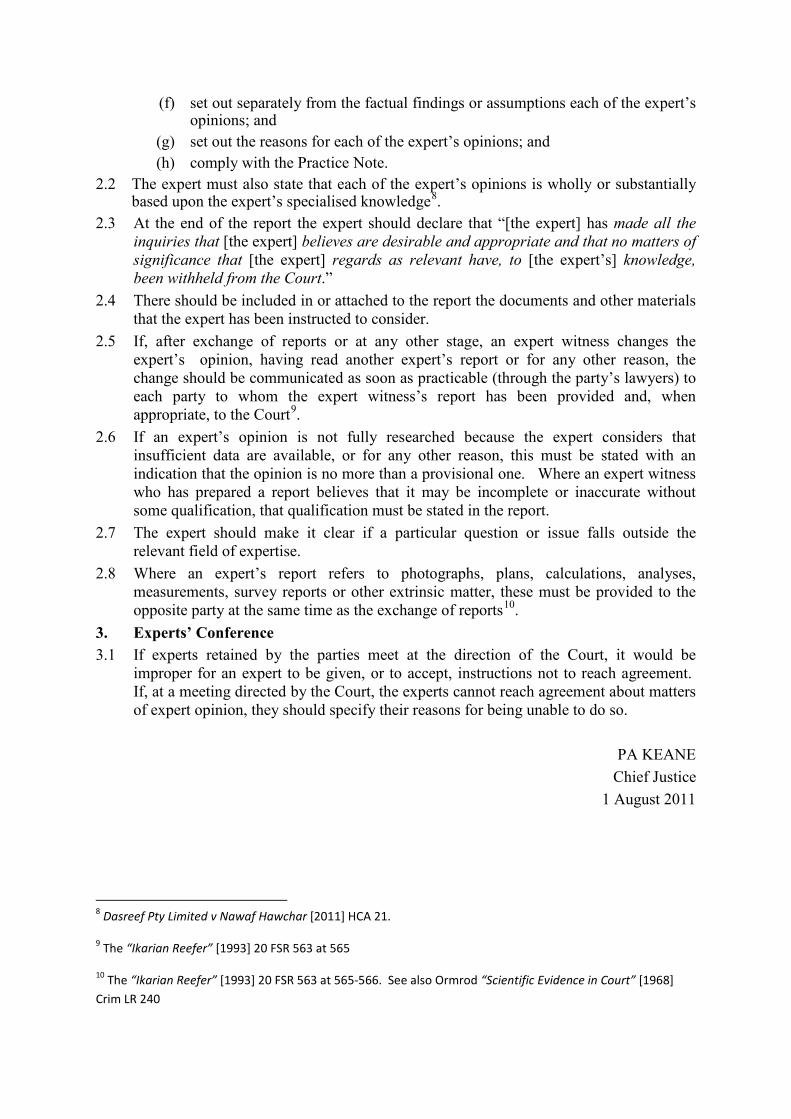
(f) set out separately from the factual findings or assumptions each of the expert’s opinions; and
(g) set out the reasons for each of the expert’s opinions; and (h) comply with the Practice Note. 2.2 The expert must also state that each of the expert’s opinions is wholly or substantially
based upon the expert’s specialised knowledge8. 2.3 At the end of the report the expert should declare that “[the expert] has made all the
inquiries that [the expert] believes are desirable and appropriate and that no matters of significance that [the expert] regards as relevant have, to [the expert’s] knowledge, been withheld from the Court.”
2.4 There should be included in or attached to the report the documents and other materials that the expert has been instructed to consider.
2.5 If, after exchange of reports or at any other stage, an expert witness changes the expert’s opinion, having read another expert’s report or for any other reason, the change should be communicated as soon as practicable (through the party’s lawyers) to each party to whom the expert witness’s report has been provided and, when appropriate, to the Court9.
2.6 If an expert’s opinion is not fully researched because the expert considers that insufficient data are available, or for any other reason, this must be stated with an indication that the opinion is no more than a provisional one. Where an expert witness who has prepared a report believes that it may be incomplete or inaccurate without some qualification, that qualification must be stated in the report.
2.7 The expert should make it clear if a particular question or issue falls outside the relevant field of expertise.
2.8 Where an expert’s report refers to photographs, plans, calculations, analyses, measurements, survey reports or other extrinsic matter, these must be provided to the opposite party at the same time as the exchange of reports10.
3. Experts’ Conference 3.1 If experts retained by the parties meet at the direction of the Court, it would be
improper for an expert to be given, or to accept, instructions not to reach agreement. If, at a meeting directed by the Court, the experts cannot reach agreement about matters of expert opinion, they should specify their reasons for being unable to do so.
PA KEANE
Chief Justice 1 August 2011
8 Dasreef Pty Limited v Nawaf Hawchar [2011] HCA 21.
9 The “Ikarian Reefer” [1993] 20 FSR 563 at 565
10 The “Ikarian Reefer” [1993] 20 FSR 563 at 565-566. See also Ormrod “Scientific Evidence in Court” [1968] Crim LR 240