Brigham Young UniversityBYU ScholarsArchive

All Theses and Dissertations

2017-05-01

Diversity and Efficiency: An Unexpected ResultJoseph Smith JohnsonBrigham Young University

Follow this and additional works at: https://scholarsarchive.byu.edu/etd

Part of the Computer Sciences Commons

This Thesis is brought to you for free and open access by BYU ScholarsArchive. It has been accepted for inclusion in All Theses and Dissertations by anauthorized administrator of BYU ScholarsArchive. For more information, please contact scholarsarchive@byu.edu, ellen_amatangelo@byu.edu.

BYU ScholarsArchive CitationJohnson, Joseph Smith, "Diversity and Efficiency: An Unexpected Result" (2017). All Theses and Dissertations. 6359.https://scholarsarchive.byu.edu/etd/6359

Diversity and Efficiency: An Unexpected Result

Joseph Smith Johnson

A thesis submitted to the faculty ofBrigham Young University

in partial fulfillment of the requirements for the degree of

Master of Science

Christophe Giraud-Carrier, ChairTony R. Martinez

Yiu-Kai Ng

Department of Computer Science

Brigham Young University

Copyright c© 2017 Joseph Smith Johnson

All Rights Reserved

ABSTRACT

Diversity and Efficiency: An Unexpected Result

Joseph Smith JohnsonDepartment of Computer Science, BYU

Master of Science

Empirical evidence shows that ensembles with adequate levels of pairwise diversityamong a set of accurate member algorithms significantly outperform any of the individualalgorithms. As a result, several diversity measures have been developed for use in optimizingensembles. We show that diversity measures that properly combine the diversity spacein an additive and multiplicative manner, not only result in ensembles whose accuracy iscomparable to the naıve ensemble of choosing the most accurate learners, but also resultsin ensembles that are significantly more efficient than such naıve ensembles. In addition todiversity measures found in the literature, we submit two measures of diversity that span thediversity space in unique ways. Each of these measures considers not only the diversity ofratings between a pair of algorithms, but how this diversity relates to the target values.

Keywords: Diversity measures, ensembles, metalearning

ACKNOWLEDGMENTS

Thanks go to Chris Monson for the LATEX template. We also wish to acknowledge

New York University (http://lib.stat.cmu.edu/datasets/) and the University of California,

Irvine (http://archive.ics.uci.edu/ml/) for their excellent dataset repositories. We would

also like to acknowledge the University of Waikado for permission to use it’s tool, weka,

(http://www.cs.waikato.ac.nz/ml/weka/). The website for weka includes additional links to

other datasets (https://weka.wikispaces.com/Datasets) that may be helpful to the interested

reader.

Table of Contents

List of Figures vi

List of Tables viii

1 Introduction 1

1.1 Measure For Optimal Ensemble Diversity . . . . . . . . . . . . . . . . . . . . 2

1.2 Voted Ensemble . . . . . . . . . . . . . . . . . . . . . . . . . . . . . . . . . . 3

1.3 Stacking Ensemble . . . . . . . . . . . . . . . . . . . . . . . . . . . . . . . . 4

2 Related Work 6

3 Identifying How Diversity Affects Accuracy 9

3.1 “Right” Diversity . . . . . . . . . . . . . . . . . . . . . . . . . . . . . . . . . 9

3.2 Proposed Solutions . . . . . . . . . . . . . . . . . . . . . . . . . . . . . . . . 10

4 Test Set-up 12

4.1 Test Data . . . . . . . . . . . . . . . . . . . . . . . . . . . . . . . . . . . . . 12

4.2 Ensemble Optimization . . . . . . . . . . . . . . . . . . . . . . . . . . . . . . 14

5 Results 15

5.1 Results . . . . . . . . . . . . . . . . . . . . . . . . . . . . . . . . . . . . . . . 15

5.2 Results . . . . . . . . . . . . . . . . . . . . . . . . . . . . . . . . . . . . . . . 26

6 Conclusions 36

6.1 Future work . . . . . . . . . . . . . . . . . . . . . . . . . . . . . . . . . . . . 36

iv

References 39

Appendix A Visual Representation of Relationship Between Accuracy and

Diversity 40

Appendix B Results of Selected Algorithms Applied to 164 Datasets 42

v

List of Figures

5.1 Classification rates and execution times (most expensive base learner) of

Voting(DF ) and Voting(accuracy) according to classification rates of best

classifier . . . . . . . . . . . . . . . . . . . . . . . . . . . . . . . . . . . . . . 20

5.2 Classification rates and execution times (most expensive base learner) of

Voting(DF ) and Voting(accuracy) according to number of instances . . . . . 21

5.3 Classification rates and execution times (most expensive base learner) of

Voting(DF ) and Voting(accuracy) according to number of features . . . . . 22

5.4 Classification rates and execution times (most expensive base learner) of

Voting(DF ) and Voting(accuracy) according to number of classes . . . . . . 23

5.5 Classification rates and execution times (most expensive base learner) of

Voting(DF ) and Voting(accuracy) according to number of learners in common 24

5.6 Classification rates and execution times (most expensive base learner) of

Voting(DF ) and Voting(accuracy) according to classification rates of best

classifier . . . . . . . . . . . . . . . . . . . . . . . . . . . . . . . . . . . . . . 30

5.7 Classification rates and execution times (most expensive base learner) of

Voting(DF ) and Voting(accuracy) according to number of instances . . . . . 31

5.8 Classification rates and execution times (most expensive base learner) of

Voting(DF ) and Voting(accuracy) according to number of features . . . . . 32

5.9 Classification rates and execution times (most expensive base learner) of

Voting(DF ) and Voting(accuracy) according to number of classes . . . . . . 33

vi

5.10 Classification rates and execution times (most expensive base learner) of

Voting(DF ) and Voting(accuracy) according to number of learners in common 34

A.1 A graphical depiction of how the spaces spanned by ensembles better ap-

proximate the signal f than the individual classifiers. Figure taken from

[1]. . . . . . . . . . . . . . . . . . . . . . . . . . . . . . . . . . . . . . . . . . 41

A.2 The accurate learners effectively approximate the true hypotheses f , but after

much training and fine-tuning. . . . . . . . . . . . . . . . . . . . . . . . . . . 41

A.3 The diverse learners do not approximate f as well as the accurate learners,

but their average approximates the function comparable to the accurate learners. 41

vii

List of Tables

1.1 A simple voting ensemble. . . . . . . . . . . . . . . . . . . . . . . . . . . . . 3

2.1 Common descriptions of the diversity space . . . . . . . . . . . . . . . . . . . 7

5.1 Top results of running ensembles on 164 datasets. . . . . . . . . . . . . . . . 16

5.2 Execution time of most expensive base learner by measure. (in seconds) . . . 17

5.3 Execution times (in seconds) of the most expensive base learner for accuracy

and DF according to the classification rates of best classifier. . . . . . . . . . 19

5.4 Top results of running ensembles on 164 datasets. . . . . . . . . . . . . . . . 27

5.5 Execution time of most expensive base learner by measure. (in seconds) . . . 27

5.6 Execution times (in seconds) of the most expensive base learner for accuracy

and DF according to the classification rates of best classifier. . . . . . . . . . 29

B.1 Accuracy and runtime for 48 base learners applied to 164 datasets. . . . . . . 43

viii

Chapter 1

Introduction

Ensemble learning consists of assembling a set of learning algorithms, providing each

algorithm with a set of data, and combining the results in clever ways so as to provide high

classification rates for a dataset D. In this sense, these computational methods resemble

musical ensembles where each instrument reads from a score of music and the combined output

is richer than the output of each individual instrument. The movement towards ensemble

learning is largely due to empirical results showing that ensembles perform significantly better

than the individual constituting algorithms [1]. However, the improved accuracy is based on

the individual learners being both accurate and diverse. Diversity can be roughly defined

as, given an arbitrary input, the degree to which two algorithms make different predictions.

Accuracy can be defined as the degree to which an algorithm has an error rate lower than

random guessing. Hence, we want a group of algorithms with high accuracy where the

predictions they make differ adequately so as to generalize optimally against new data. When

considering an ensemble of more than two algorithms, this allows a greater probability of

the group accurately predicting an instance even when a minority of the learners predict

incorrectly.

In the modern world of proliferating mobile electronics, sensors, and autonomous

machines, there are inherent limits on computational time and space. As a result, algorithms

demand a high degree of robustness, accuracy, and efficiency. Ensembles provide such a

solution. However, given that time and space complexity are the limiting constraints, large

ensembles containing several complex base learners are prohibitively expensive. As a result,

1

an effective diversity measure for optimizing ensembles will hold execution times at a certain

level while maximizing accuracy. This study will first focus on how varying diversity measures

take into account different compositions of diversity and accuracy. We will then create

ensembles that have been optimized by these measures and compare their classification rates

and running times. We will show that diversity buys efficiency while maintaining a level

of accuracy comparable to the naıve method of creating an ensemble by choosing the most

accurate base learners.

1.1 Measure For Optimal Ensemble Diversity

Given the dual criteria of ensembles possessing accurate base learners as well as those base

learners having high pairwise diversity, one would gravitate towards developing measures or

selecting existing measures that favor simultaneously high levels of pairwise diversity and

accuracy among the learners. We want to ensure that such measures would not allow high

accuracy to somehow compensate for poor diversity. Given that no algorithm is superior to

all other algorithms over all classification tasks, greatly reducing diversity among learners in

favor of accuracy would not effectively span the classification space. We need learners that

have a more orthogonal relationship where the union of their collective predictions maximally

intersects with the true class while minimally overlapping when predicting the wrong class.

We then will test to see whether these measures outperform simple maximal diversity or

simple maximal accuracy.

Given that ensemble methods come in many different forms, the natural question to

ask is what composition of diversity and accuracy does each method favor? For example, the

simple voted ensemble gives equal weight to each learner. Too much diversity among the base

learners may lead to a consensus that is not in line with the true class. One is tempted to

think that accuracy would hold relatively more weight than diversity for the voted ensemble.

On the other hand, a stacking ensemble has more flexibility in weighting the base learners.

One would think diversity would hold more weight for this method than for voting. In order

2

Alg 1 Vote Alg 2 Vote Alg 3 Vote Ensemble VoteInstance1Instance2Instance3

Table 1.1: A simple voting ensemble.

to explore how diversity and accuracy affect different ensemble methods, we will apply our

diversity measures to two previously mentioned methods.

One important element of the ensembles we tested is that they are mixed ensembles.

Each ensemble consists of unique base learners. In doing so, we use diversity as a measure

of the base learner outputs. It is common to use an ensemble of homogenous base learners

where the hyperparamaters of the training data are adjusted to provide diverse inputs. We

leave the hyperparameters unchanged from base learner to base learner.

1.2 Voted Ensemble

The voted ensemble is arguably the simplest of the ensemble methods. A set of algorithms A

is assembled and each algorithm a ∈ A is trained on a training set T and produces predictions

for each instance di of a dataset D whose target classes Y are unknown. For each instance

d ∈ D, a consensus is formed among the algorithms as to what the “group” vote is. The

most common form of arriving at the consensus is a simple vote where the class that receives

the most votes becomes the consensus class. The consensus class for each instance becomes

the ensembles predicted class. Table I shows a simple representation of how such a consensus

is arrived at for a dataset containing three classes; yellow, red, and green.

We note the specifics of the voted ensemble in pseudo code. Let T be a training set of

data, {A1, A2, ..., AN} be a set of N classifiers, Y be a finite set of target class values and σ

be the generalized Kronecker function (σ(a, b) = 1 if a = b; 0 otherwise). The pseudo-code

for the voted ensemble is as follows:

3

1. For k = 1 to N

a. hk = model induced by Ak from T

2. For each new query instance q

a. Class(q) = argmaxy∈Y∑N

k=1 σ(y, hi(q))

As mentioned above, the voted ensemble gives equal weight to all members of the

ensemble for each instance. This would tend to favor learners with high accuracy over high

pairwise diversity.

1.3 Stacking Ensemble

The stacking ensemble essentially creates an entirely new dataset that is comprised of the

classifications of each of the member learners for each instance [? ]. A separate learner,

termed the metalearner, then classifies each new instance based on this new dataset of base

learner classifications.

Let T be the base-level training set, N be the number of base-level learning algorithms,

{A1, A2, ..., AN} be the set of base-level learning algorithms, Ek be an instance consisting

of all classifications made by base learners for instance k and the target class yk, τ be the

induced dataset consisting of all instances Ek, and Ameta be the chosen meta-level learner.

The pseudo code for stacking is as follows:

1. For i = 1 to N

a. hi = model induced by Ai from T

2. τ = ∅

a. For k = 1 to |T |

3. Ek =< h1(xk), h2(xk), ..., hN(xk), yk >

a. τ = τ⋃{Ek}

4. hmeta = model induced by Ameta from τ

4

a. For each new query instance q

5. Class (q) = hmeta(< h1(q), h2(q), ..., hN(q) >)

Stacking ensembles generally come in two forms. The most basic form creates a

metadataset that is comprised simply of the base learner class predictions for each instance.

This form is called simple stacking. A more sophisticated form will add the original instance

features to the base learner class predictions. We will focus exclusively on simple stacking.

5

Chapter 2

Related Work

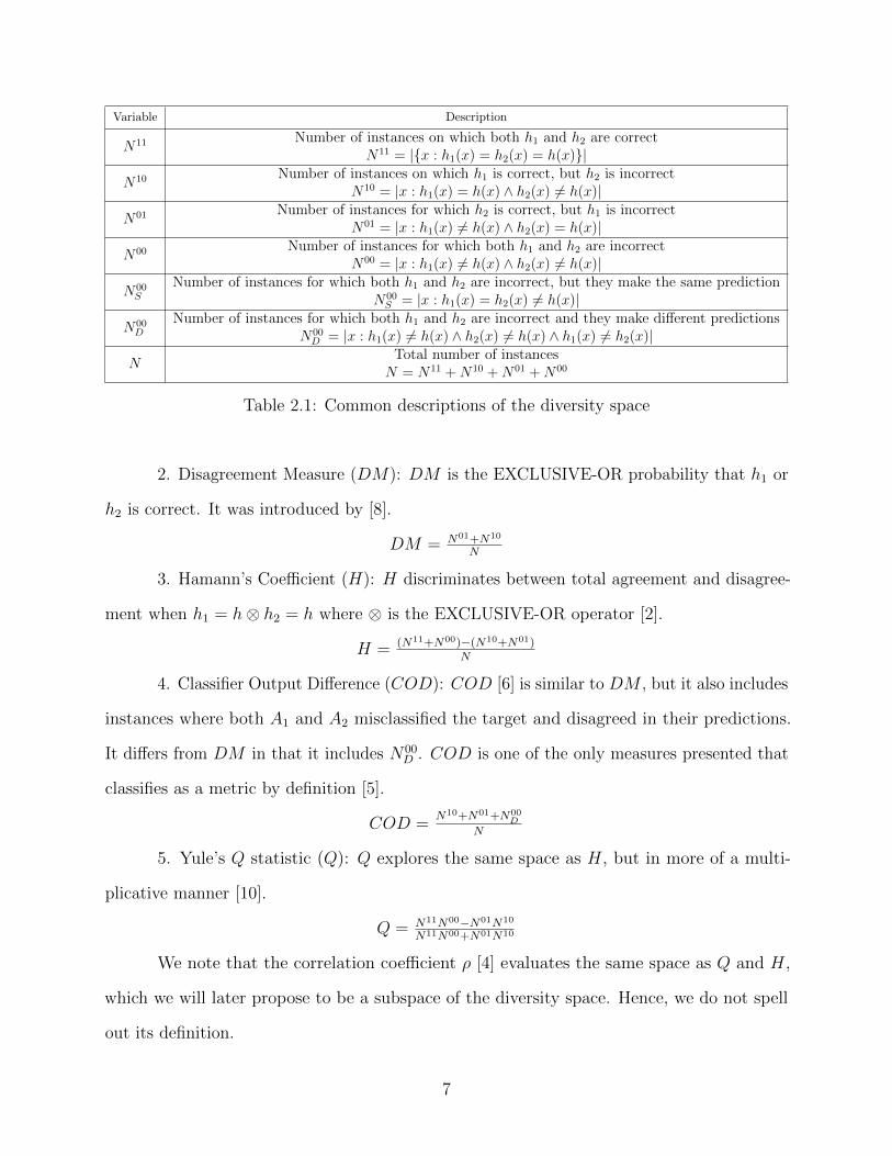
There is abundant research on diversity measures for classifiers. We propose definitions

to motivate our discussion throughout the paper based on [5] that describe pairwise diversity.

Let A1 and A2 be two learning algorithms and h be the target classification hypothesis. Let

the hypotheses h1 and h2 be those induced by A1 and A2, respectively. Table II describes

the relationships we will explore. As a brief summary of the table, let x = 1 refer to A1

correctly classifying an instance and x = 0 be otherwise. We define y in the same manner for

A2. Nxy refers to the number of instances in which x and y are both the case. For example,

N10 refers to the number of instances in which A1 correctly classifies an instance while A2

does not. Note that there are two forms of N00. N00S refers to the number of instances where

A1 and A2 misclassify an example in which they both predict that same class. N00D refers to

the number of instances where the two algorithms both misclassify an instance, but their

predicted classes are different. Hence, N00 = N00S +N00

D .

We briefly introduce a few diversity measures proposed in the literature.

1. Double Fault (DF ): This is the probability that h1 and h2 are both incorrect [3].

DF = N00

N

For the purpose of this study the phrases “minimizing DF” and “maximizing (1−DF )”

will be synonymous with “optimizing DF”. Note that optimizing this measure indirectly

optimizes accuracy, because each portion of the diversity space includes an instance where at

least one of the learners had a correct classification.

6

Variable Description

N11 Number of instances on which both h1 and h2 are correctN11 = |{x : h1(x) = h2(x) = h(x)}|

N10 Number of instances on which h1 is correct, but h2 is incorrectN10 = |x : h1(x) = h(x) ∧ h2(x) 6= h(x)|

N01 Number of instances for which h2 is correct, but h1 is incorrectN01 = |x : h1(x) 6= h(x) ∧ h2(x) = h(x)|

N00 Number of instances for which both h1 and h2 are incorrectN00 = |x : h1(x) 6= h(x) ∧ h2(x) 6= h(x)|

N00S

Number of instances for which both h1 and h2 are incorrect, but they make the same predictionN00

S = |x : h1(x) = h2(x) 6= h(x)|

N00D

Number of instances for which both h1 and h2 are incorrect and they make different predictionsN00

D = |x : h1(x) 6= h(x) ∧ h2(x) 6= h(x) ∧ h1(x) 6= h2(x)|

NTotal number of instancesN = N11 +N10 +N01 +N00

Table 2.1: Common descriptions of the diversity space

2. Disagreement Measure (DM): DM is the EXCLUSIVE-OR probability that h1 or

h2 is correct. It was introduced by [8].

DM = N01+N10

N

3. Hamann’s Coefficient (H): H discriminates between total agreement and disagree-

ment when h1 = h⊗ h2 = h where ⊗ is the EXCLUSIVE-OR operator [2].

H = (N11+N00)−(N10+N01)N

4. Classifier Output Difference (COD): COD [6] is similar to DM , but it also includes

instances where both A1 and A2 misclassified the target and disagreed in their predictions.

It differs from DM in that it includes N00D . COD is one of the only measures presented that

classifies as a metric by definition [5].

COD =N10+N01+N00

D

N

5. Yule’s Q statistic (Q): Q explores the same space as H, but in more of a multi-

plicative manner [10].

Q = N11N00−N01N10

N11N00+N01N10

We note that the correlation coefficient ρ [4] evaluates the same space as Q and H,

which we will later propose to be a subspace of the diversity space. Hence, we do not spell

out its definition.

7

6. Two types of Error Correlation (EC) are cited in [5]; ECa and ECk. ECa is

similar to DF but does not include N00D . ECk is similar to ECa, but it excludes N11 in the

denominator.

ECa =N00

S

N

ECk =N00

S

N01+N10+N00

We show that, of the measures shown above, DF is the most effective in terms of

accuracy while COD is the most efficient in terms of running time.

8

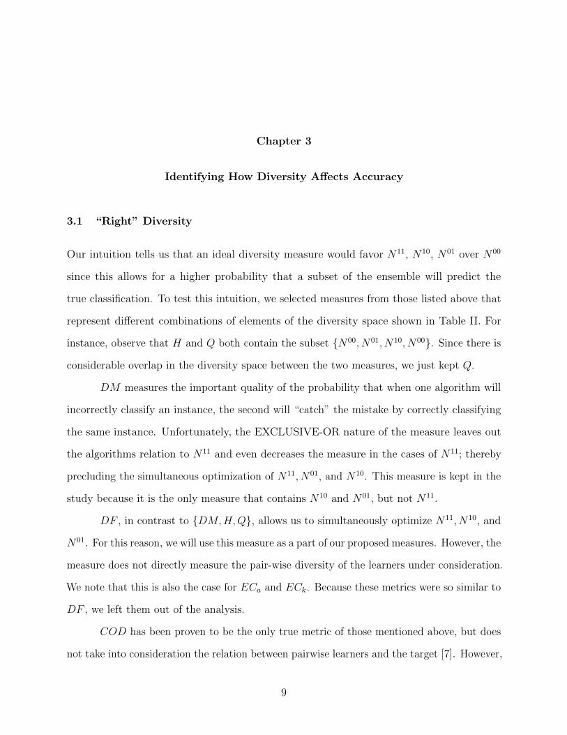
Chapter 3

Identifying How Diversity Affects Accuracy

3.1 “Right” Diversity

Our intuition tells us that an ideal diversity measure would favor N11, N10, N01 over N00

since this allows for a higher probability that a subset of the ensemble will predict the

true classification. To test this intuition, we selected measures from those listed above that

represent different combinations of elements of the diversity space shown in Table II. For

instance, observe that H and Q both contain the subset {N00, N01, N10, N00}. Since there is

considerable overlap in the diversity space between the two measures, we just kept Q.

DM measures the important quality of the probability that when one algorithm will

incorrectly classify an instance, the second will “catch” the mistake by correctly classifying

the same instance. Unfortunately, the EXCLUSIVE-OR nature of the measure leaves out

the algorithms relation to N11 and even decreases the measure in the cases of N11; thereby

precluding the simultaneous optimization of N11, N01, and N10. This measure is kept in the

study because it is the only measure that contains N10 and N01, but not N11.

DF , in contrast to {DM,H,Q}, allows us to simultaneously optimize N11, N10, and

N01. For this reason, we will use this measure as a part of our proposed measures. However, the

measure does not directly measure the pair-wise diversity of the learners under consideration.

We note that this is also the case for ECa and ECk. Because these metrics were so similar to

DF , we left them out of the analysis.

COD has been proven to be the only true metric of those mentioned above, but does

not take into consideration the relation between pairwise learners and the target [7]. However,

9

we conjecture that a method that combines DF and COD is an effective approach to the

multi-objective optimization of diversity and accuracy in ensembles.

We feel that the measures {COD,DF,DM,Q} represent important subsets of the

diversity space. This representation will help us understand what subset of the diversity space

is most important. Since we do not believe that the aforementioned measures exhaustively

represent the most critical subspaces of the diversity subspace, we develop two measures next.

3.2 Proposed Solutions

As part of this study, we propose two measures that we feel strike an optimal balance between

diversity and complexity and that complement the existing set of measures mentioned above.

First, we propose a search process that entails initially ranking in ascending order a set of

ensembles by their average pairwise DF . We chose DF because the measure implies a certain

level of accuracy and diversity. If we were to simply rank the ensembles according to the

average accuracy of their base learners, we could not ensure that there would be a relatively

higher score of N00 as opposed to the more favorable regions of N10 and N01. The next step

in the process chooses the top k ensembles and selects the ensemble with the highest average

pairwise COD.

This process serves the dual purpose of maximizing accuracy and diversity, but

prioritizes accuracy in the search. The justification for giving priority to accuracy is that an

ensemble can generally do no worse than its least accurate member algorithm, if the least

accurate algorithm has a better classification rate than a random guess. This is the case

even with minimal diversity. However, an ensemble in which the member algorithms make

uncorrelated errors at a rate higher than a random guess will increase the error rate of the

ensemble [1]. We will refer to this measure as sorted, given that the step that differentiates

this measure from DF is when the top k ensembles are sorted by COD and the top ensemble

chosen. We use k = 1000 for our experiment.

10

We propose a second measure that additively combines accuracy and COD. Specifically,

for a set of algorithms A = {a1, a2, , an} and a training set T , we combine accuracy and

COD:

αvoted(A) + (1− α)cod(A)

where voted(A) calculates the accuracy of the voted ensemble using A over T , cod(A) calculates

CODpairwiseaverage for all pairs of algorithms in A and α can be adjusted to give one measure

weight over the other. (For the purposes of our experiments, α = 0.5) We have a similar

approach for stacking ensembles:

αstacking(A,M) + (1− α)cod(A)

where stacking(A,M) refers to the accuracy of employing the stacking method on T while

using the metalearner M . We will call this method composite given that it melds accuracy

and diversity.

We seek to compare the accuracy on the voted ensemble and stacking ensemble when

employing our proposed methodologies to optimized levels of overall accuracy, DF , DM , and

H. Note that optimizing on overall accuracy entails choosing the base learners that have the

highest classification rates for T . We will refer to this as accuracy. As mentioned above, we

specifically choose these measures because they each constitute a particular representation

of the diversity space. We also compare the results to the base methodology of creating an

ensemble through a random choice of algorithms that we will refer to as random.

11

Chapter 4

Test Set-up

4.1 Test Data

We chose many different types of datasets in order for our results to be robust. We used 164

datasets pulled from different sources; primarily the excellent datasets available in the UCI

Machine Learning Repository (http://archive.ics.uci.edu/ml/) and from New York University

(http://lib.stat.cmu.edu/datasets/). We also use datasets that are available with the weka

download (http://www.cs.waikato.ac.nz/ml/weka/). For each dataset, we will apply 10-fold

cross-validation. In this cross-validation, the ensembles will be optimized on the 9 folds and

tested on the left out fold. It is critical to note that each selection of folds forms an instance

in a metadataset. Hence, there are 10x164 instances in the metadataset. Each instance will

include as features the classification rate and execution time of the base learners for the

best ensembles according to DM,DF,H, accuracy, COD, and the approximately optimized

ensembles according to our two proposed methods. These ensembles are created by using all

instances in the 9 training folds to optimize ensembles according to our set of measures. The

ensembles are evaluated on the hold-out test fold and the classification rate is recorded. As

mentioned above, the hyperparameters of the traning data do not change from base learner

to base learner nor from ensemble to ensemble.

We focus on the execution times of the base learners in an ensemble. We also isolate

the running time of the base learners in order to highlight how expensive the algorithms are

that are chosen by different metrics. There would be additional slight overhead for the voting

mechanism and potentially more for the Stacking metalearner. However, a focus on the base

12

learners allows us to focus on that which the diversity measures can control. In addition, we

represent the running time as the maximum running time given a metric M for an ensemble

A = {A1, A2, ..., Ak} run on instance i. Then the average running time for M over the entire

metadataset of n samples becomes:

1n

∑n1 max{xij : xij is runtime for aj ∈ A on instance i}

The execution times are based on a pre-trial where each algorithm was passed through

each dataset. This provides uniformity by avoiding the case where an arbitrary algorithm

records different running time when used in two different ensembles.

Base learners can be run in parallel. Hence, the bottleneck in the classification process

will be waiting for the slowest base learner to terminate.

We test ensembles of size 5. This size was chosen since it constitutes a small percentage

of the 48 algorithms we used in this study and will not result in high degrees of base learner

overlap among ensembles. (Please see Appendix B for a list of the base learners and the

results of running the learners on the 164 datasets.) We found that as the size of the ensemble

grows with respect to the number of algorithms available, the difference in the accuracy of

the best and worst ensembles starts to shrink.

For each fold that is classified, we will select the single learner with the highest accuracy

to serve as a benchmark. This idea was used effectively in [4]. The learner and its accuracy

will be recorded for the particular fold. This will be referred to as best classifier throughout

the analysis of the test results. Please keep in mind that the best classifier generally changes

from instance to instance and does not refer to the single best classifier over all the datasets.

However, it does give one a notion of how “hard” the particular fold is to classify.

For the stacking ensemble, we used weka implementations of the J.48 decision tree,

Naıve Bayes, and the Multi-Layer Perceptron as metalearners. (See http://www.cs.waikato.ac.nz/ml/weka/)

We will refer to them as tree, bayes, and mlp, respectively. We never mixed metalearners for

a given ensemble. We ran the metalearners separately on each optimized ensemble.

13

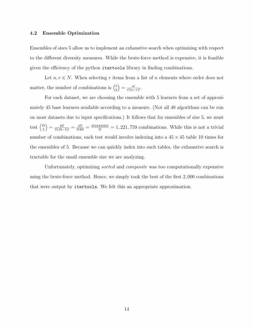
4.2 Ensemble Optimization

Ensembles of sizes 5 allow us to implement an exhaustive search when optimizing with respect

to the different diversity measures. While the brute-force method is expensive, it is feasible

given the efficiency of the python itertools library in finding combinations.

Let n, r ∈ N . When selecting r items from a list of n elements where order does not

matter, the number of combinations is(nk

)= n!

r!(n−r)! .

For each dataset, we are choosing the ensemble with 5 learners from a set of approxi-

mately 45 base learners available according to a measure. (Not all 48 algorithms can be run

on most datasets due to input specifications.) It follows that for ensembles of size 5, we must

test(455

)= 45!

5!(45−5)! = 45!5!40!

= 45444342415!

= 1, 221, 759 combinations. While this is not a trivial

number of combinations, each test would involve indexing into a 45× 45 table 10 times for

the ensembles of 5. Because we can quickly index into such tables, the exhaustive search is

tractable for the small ensemble size we are analyzing.

Unfortunately, optimizing sorted and composite was too computationally expensive

using the brute-force method. Hence, we simply took the best of the first 2, 000 combinations

that were output by itertools. We felt this an appropriate approximation.

14

Chapter 5

Results

5.1 Results

Table III shows the results of the top performing ensembles overall on the 1, 640 instance

metadataset. The notation Voting(measure) refers to the performance of the simple ma-

jority voting algorithm for ensembles that have been created by optimizing measure ∈

{accuracy, COD,DF, ...}. With stacking, the notation is Stacking(measure,metalearner)

wheremeasure comes from the same set as that of Voting andmetalearner ∈ {bayes, tree,mlp}.

For purposes of comparison, the results of the best classifier, as well as the top random

ensemble and the top single algorithm were included. The single algorithm selected was the

algorithm with the highest overall classification rate and had classified all datasets. (21 of

the available 49 algorithms could not classify every dataset. Also keep in mind that this is

different than best classifier.)

The top ensembles outperformed the best average single classifier (trees.LMT ) by

nearly 10% and came within 2% of best classifier. Also, 11 of the 32 ensembles outperformed

the best overall single classifier. The results show accuracy and DF to be the measures

employed by the top 7 ensembles. These two measures fully take into account N11 while DM

and COD do not and the N11 score by H can be offset by high N10 and N01 scores. These

results suggest that from an accuracy point-of-view, N11 is the most important region of the

diversity space.

Interestingly, ensembles optimized for accuracy (those optimized by accuracy, DF ,

and sorted) and those optimized for diversity (ensembles optimized by COD) lie at opposite

15

Measure Mean Median Standard Deviation

bestclassifier 80.86% 85.54% 17.49%Voting(accuracy) 78.57% 84.57% 22.29%Stacking(accuracy, bayes) 78.33% 83.33% 22.61%Voting(DF ) 78.03% 83.33% 22.39%Stacking(DF , bayes) 78.03% 83.33% 22.86%Stacking(accuracy, tree) 77.82% 83.33% 22.84%Stacking(accuracy, mlp) 77.27% 83.33% 23.36%Stacking(DF , tree) 77.08% 83.33% 23.25%Stacking(sorted, bayes) 77.02% 82.55% 23.02%Voting(sorted) 76.58% 82.14% 23.09%Stacking(composite, bayes) 76.47% 81.53% 22.90%... ... ... ...trees.LMT 76.53% — —... ... ... ...Stacking(Random, bayes) 76.15% 81.48% 23.26%... ... ... ...Voted(random) 74.40% 80.00% 23.61%... ... ... ...Average Single Classifier 70.49% — —... ... ... ...Voting(COD) 65.03% 70.00% 25.75%

Table 5.1: Top results of running ensembles on 164 datasets.

16

Measure Mean Median Standard Deviation

accuracy 2.72 0.27 6.51DF 2.27 0.26 5.83sorted 2.00 0.18 5.45Random 1.44 0.18 4.64DM 0.97 0.09 3.43composite 0.92 0.14 2.91H 0.87 0.09 3.00COD 0.46 0.07 2.06

Table 5.2: Execution time of most expensive base learner by measure. (in seconds)

extremes of Table III. This shows that diversity is desirable but cannot stand alone. With

this in mind, one may be tempted to think that diversity does not significantly enhance an

ensemble and that the naıve method of selecting the most accurate learners is preferable.

However, the right diversity does enhance the ensemble in an unexpected way; it improves

the execution time while maintaining essentially the same accuracy.

Table IV shows the overall average execution times of the slowest of the base learners

chosen by the different measures. From the table it becomes apparent that the three

measures with the most accurate ensembles (accuracy,DF, sorted) are also the most expensive

computationally. This is because it is generally the case that accurate base learners require

more time and resources to learn patterns from datasets. DF , accuracy and sorted explicitly

select accurate learners. These measures directly target the N11,N10, and N01 regions of

the diversity space. DM and COD do not directly select accurate learners while H and

composite may bypass accurate learners in favor of learners with more pairwise diversity.

They pay a price as far as accuracy, but are much more efficient.

This leads us to believe there is a relationship between diversity and efficiency. Gen-

erally speaking, relatively high accuracy is a result of a given algorithm’s ability to exploit

non-linear decision boundaries or perform a more exhaustive search in the hypothesis space of

a dataset than a simpler learner. This implies longer runtimes. Diversity discourages inclusion

of the most accurate learners for a given dataset, because this would necessitate finding very

17

poor learners in order to obtain high pairwise diversity. As a result, the base learners of an

ensemble that is optimized by a diversity measure will tend to have less computationally

expensive learners. However, from Tables III and V we note that DF was able to achieve

lower running times while maintaining classification rates comparable to accuracy. Table IV

shows that accuracy was 20%, 5.7%, 11.5% greater than DF as far as mean, median, and

standard deviation of execution times, respectively. The ensembles optimized by DF in Table

III are comparable to accuracy in terms of classification rate. DF maintains this accuracy

by directly targeting N10 and N01 while excluding N00. The previous results suggest that

the regions N01 and N10 are most useful in terms of efficiency. They create diversity in the

ensemble, which indirectly generates efficiency, while maintaining a level of accuracy.

While these results point to a general relationship between diversity and efficiency, a

closer look at how the base learner execution times for accuracy and DF compare with respect

to data regularity reveals cases where accuracy may be more efficient. We will restrict our

analysis to Voting(accuracy) and Voting(DF ) since these were the most accurate ensembles.

Regularity is an abstract term referring to the degree to which well-structured patterns exist

in the data. Because there is no particular measure of regularity, we will use the classification

rate of best classifier as an indicator of structure. The assumption is simple; the higher the

classification rate of best classifier, the “easier” it is to detect patterns in the data. Table V

partitions the data according to the instances that fall within a certain accuracy range of

best classifier. For example, all 249 instances where best classifier ’s classification rate was

between [.95, 1) were grouped together and analyzed separately. Note that the bin labeled

“100%” refers to the instances where best classifier had 100% accuracy. The support refers to

the number of instances in each particular bin.

The table shows that DF generally classified as well as accuracy and exhibited lower

execution times. With the exception of the bins representing 100% and 25-40%, the DF

classification rates were not significantly different than those of accuracy. The execution

times, however, differed according to the level of regularity. The bottom graph of Figure 1

18

Bin Support Mean Execution DF Mean Execution accuracy Mean Class. Rate DF Mean Class. Rate accuracy Margin

100% 120 0.77 2.08 97.43% 99.7% -2.27%95% 249 3.32 5.38 96.28% 96.32% -0.05%90% 177 2.04 2.48 89.35% 88.91% 0.44%85% 319 1.68 1.84 84.11% 85.41% -1.3%80% 206 4.30 4.98 81.43% 80.92% 0.5%75% 115 1.04 1.30 76.18% 77.3% -1.12%70% 135 1.83 1.11 70.04% 70.28% -0.24%65% 64 4.29 4.16 58.99% 59.58% -0.59%60% 46 2.15 2.26 60.22% 61.42% -1.2%55% 39 2.69 1.41 52.26% 53.92% -1.66%50% 38 0.40 0.33 44.34% 43.6% 0.74%45% 24 0.50 0.48 46.36% 42.79% 3.57%40% 37 1.24 0.30 36.35% 36.89% -0.54%35% 24 0.18 0.22 31.67% 34.17% -2.5%30% 26 2.60 1.15 30.28% 32.39% -2.11%25% 12 1.76 2.04 27.08% 29.19% -2.11%20% 11 1.12 1.32 21.03% 21.72% -0.69%

Table 5.3: Execution times (in seconds) of the most expensive base learner for accuracy andDF according to the classification rates of best classifier.

shows that execution times of DF were generally greater than those of accuracy for < 0.6

and generally lower for > 0.6. At lower levels of regularity accuracy seems to be intentionally

choosing higher error bias, simpler algorithms because such algorithms increase accuracy,

while DF is leaning towards relatively lower error bias, more expensive algorithms. This

occurs with DF because it has the latitude to choose less accurate algorithms as long as

there is enough diversity in the ensemble such that the number of instances in N10 and N01

is significantly higher than those in N00. These results suggest that for datasets that tend

towards lower classification rates, there is computational savings in using accuracy. However,

for more separable, regular datasets it pays computationally to use DF .

We now consider how accuracy and DF perform against other circumstances. We will

continue to restrict our analysis to Voting(accuracy) and Voting(DF ). When considering

accuracy, we will compare performance to two ensembles that represent the lower and upper

bounds of classification. The lower bound will be represented by Voting(random). This is

the baseline that any useful method should clear. For the upper bound, we will show the

results of whichever method was most accurate for a given instance; which we will call best

19

0.2 0.4 0.6 0.8 1

0.2

0.4

0.6

0.8

1

Classification Rate for best classifier

Cla

ssifi

cati

onR

ate DF

accuracy

0.2 0.4 0.6 0.8 10

2

4

Classification Rate for best classifier

Ave

rage

Exec

uti

onT

ime

(Sec

onds)

DFaccuracy

Figure 5.1: Classification rates and execution times (most expensive base learner) ofVoting(DF ) and Voting(accuracy) according to classification rates of best classifier

20

0 100 200 300 400 500 600 700

0.7

0.8

0.9

1

Number of Instances

Cla

ssifi

cati

onR

ate

DF

accuracy

best ensemble

random

0 100 200 300 400 500 600 7000

2

4

6

8

Number of Instances

Ave

rage

Exec

uti

onT

ime

(Sec

onds)

DFaccuracy

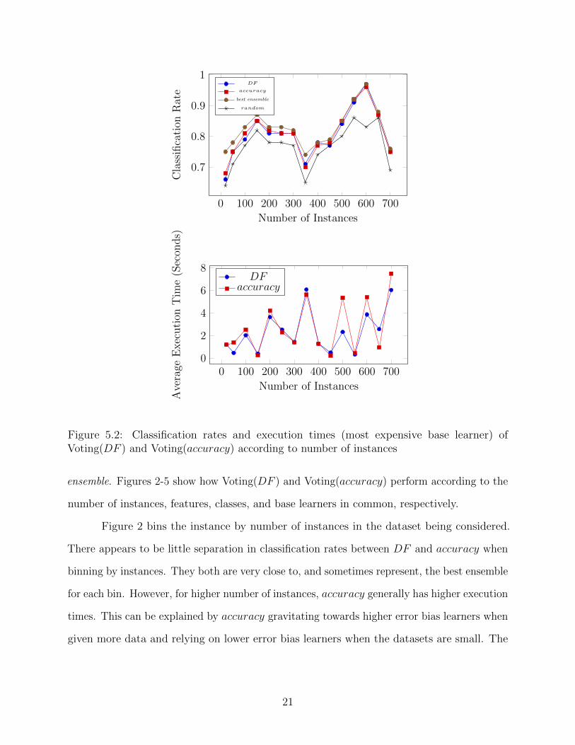
Figure 5.2: Classification rates and execution times (most expensive base learner) ofVoting(DF ) and Voting(accuracy) according to number of instances

ensemble. Figures 2-5 show how Voting(DF ) and Voting(accuracy) perform according to the

number of instances, features, classes, and base learners in common, respectively.

Figure 2 bins the instance by number of instances in the dataset being considered.

There appears to be little separation in classification rates between DF and accuracy when

binning by instances. They both are very close to, and sometimes represent, the best ensemble

for each bin. However, for higher number of instances, accuracy generally has higher execution

times. This can be explained by accuracy gravitating towards higher error bias learners when

given more data and relying on lower error bias learners when the datasets are small. The

21

0 20 40 60 80 100

0.4

0.6

0.8

Number of Features

Cla

ssifi

cati

onR

ate

DF

accuracy

best ensemble

random

0 20 40 60 80 100

0

10

20

30

Number of Features

Ave

rage

Exec

uti

onT

ime

(Sec

onds)

DFaccuracy

Figure 5.3: Classification rates and execution times (most expensive base learner) ofVoting(DF ) and Voting(accuracy) according to number of features

execution times of DF experience volatility, but do not increase by nearly as much as those

of accuracy as the number of instances increase.

Figures 3 and 4 show performance by number of features and number of classes,

respectively. We only note that the classification rates for accuracy and DF never significantly

differ. It is difficult to draw any conclusions from the execution times. The execution times

overall increase (almost exponentially), as would be expected, with an increase in the number

of classes and features.

Finally, Figure 5 shows an interesting result in which there is a distinct pattern in

classification rates and execution times with respect to the number of learners they have in

22

0 5 10 15 20 25 300.4

0.6

0.8

Number of Classes

Cla

ssifi

cati

onR

ate

DF

accuracy

best ensemble

random

0 5 10 15 20 25 30

0

10

20

30

Number of Classes

Ave

rage

Exec

uti

onT

ime

(Sec

onds)

DFaccuracy

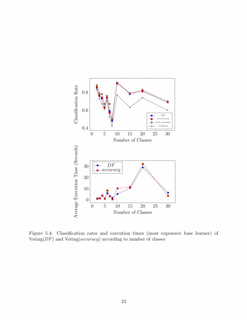
Figure 5.4: Classification rates and execution times (most expensive base learner) ofVoting(DF ) and Voting(accuracy) according to number of classes

23

0 1 2 3 4 5

0.7

0.8

0.9

Number of Base Learners in Common

Cla

ssifi

cati

onR

ate

DF

accuracy

best ensemble

random

0 1 2 3 4 5

0

5

10

15

Number of Base Learners in Common

Ave

rage

Exec

uti

onT

ime

(Sec

onds)

DFaccuracy

Figure 5.5: Classification rates and execution times (most expensive base learner) ofVoting(DF ) and Voting(accuracy) according to number of learners in common

24

common. It appears that the classification rates are highest when accuracy and DF either

have no learners in common or all learners in common. A closer look reveals that the case

where DF and accuracy have all learners in common occurred in only 9 instances. Due to the

small sample size, we will ignore the case of total overlap for DF and accuracy and note that

the classification rate decreases somewhat monotonically with the number of base learners in

common. One explanation is that simpler datasets can be classified by most any classifier.

This leads to many ensembles having relatively similar DF scores. This wide diversity of

ensembles with low DF scores increases the probability that there will be little or no overlap

with ensembles optimized for accuracy. However, as datasets become less linearly separable,

a given learner’s error bias increasingly affects its classification rate, leading to disparity in

the accuracy of the available base learners. There will be fewer base learners to choose from

and the intersection between the accuracy and DF ensembles will grow.

We mentioned in the introduction that the voted ensemble would seem to favor accuracy

over diversity and that stacking was not as unfavorable towards diversity. The results bore

out these notions. Table III shows that the ensemble with the highest average accuracy was

Voted(accuracy). On the other hand, the least accurate ensemble was Voted(COD); with a

rate of 65.03%. Interestingly, the stacking algorithms were able to produce classification rates

of 5.26%, 5.80%, and 5.90% when optimized with COD. (Results not shown in Table III.)

The two measures introduced, sorted and composite, did not perform as well as DF

and accuracy in terms of classification rates. However, three of the ensembles based on

these measures (Stacking(sorted, bayes), Voting(sorted), and Stacking(composite, bayes)) did

outperform the best individual classifier, all random ensembles and all ensembles optimized

for DM,H and COD in Table III. In addition, the run times for sorted were lower than

those of DF and accuracy, while composite ensembles had runtimes about 3 times as fast as

those for accuracy.

25

5.2 Results

Table III shows the results of the top performing ensembles overall on the 1, 640 instance

metadataset. The notation Voting(measure) refers to the performance of the simple ma-

jority voting algorithm for ensembles that have been created by optimizing measure ∈

{accuracy, COD,DF, ...}. With stacking, the notation is Stacking(measure,metalearner)

wheremeasure comes from the same set as that of Voting andmetalearner ∈ {bayes, tree,mlp}.

For purposes of comparison, the results of the best classifier, as well as the top random

ensemble and the top single algorithm were included. The single algorithm selected was the

algorithm with the highest overall classification rate and had classified all datasets. (21 of

the available 49 algorithms could not classify every dataset. Also keep in mind that this is

different than best classifier.)

The top ensembles outperformed the best average single classifier (trees.LMT ) by

nearly 10% and came within 2% of best classifier. Also, 11 of the 32 ensembles outperformed

the best overall single classifier. The results show accuracy and DF to be the measures

employed by the top 7 ensembles. These two measures fully take into account N11 while DM

and COD do not and the N11 score by H can be offset by high N10 and N01 scores. These

results suggest that from an accuracy point-of-view, N11 is the most important region of the

diversity space.

Interestingly, ensembles optimized for accuracy (those optimized by accuracy, DF ,

and sorted) and those optimized for diversity (ensembles optimized by COD) lie at opposite

extremes of Table III. This shows that diversity is desirable but cannot stand alone. With

this in mind, one may be tempted to think that diversity does not significantly enhance an

ensemble and that the naıve method of selecting the most accurate learners is preferable.

However, the right diversity does enhance the ensemble in an unexpected way; it improves

the execution time while maintaining essentially the same accuracy.

Table IV shows the overall average execution times of the slowest of the base learners

chosen by the different measures. From the table it becomes apparent that the three

26

Measure Mean Median Standard Deviation

bestclassifier 80.86% 85.54% 17.49%Voting(accuracy) 78.57% 84.57% 22.29%Stacking(accuracy, bayes) 78.33% 83.33% 22.61%Voting(DF ) 78.03% 83.33% 22.39%Stacking(DF , bayes) 78.03% 83.33% 22.86%Stacking(accuracy, tree) 77.82% 83.33% 22.84%Stacking(accuracy, mlp) 77.27% 83.33% 23.36%Stacking(DF , tree) 77.08% 83.33% 23.25%Stacking(sorted, bayes) 77.02% 82.55% 23.02%Voting(sorted) 76.58% 82.14% 23.09%Stacking(composite, bayes) 76.47% 81.53% 22.90%... ... ... ...trees.LMT 76.53% — —... ... ... ...Stacking(Random, bayes) 76.15% 81.48% 23.26%... ... ... ...Voted(random) 74.40% 80.00% 23.61%... ... ... ...Average Single Classifier 70.49% — —... ... ... ...Voting(COD) 65.03% 70.00% 25.75%

Table 5.4: Top results of running ensembles on 164 datasets.

Measure Mean Median Standard Deviation

accuracy 2.72 0.27 6.51DF 2.27 0.26 5.83sorted 2.00 0.18 5.45Random 1.44 0.18 4.64DM 0.97 0.09 3.43composite 0.92 0.14 2.91H 0.87 0.09 3.00COD 0.46 0.07 2.06

Table 5.5: Execution time of most expensive base learner by measure. (in seconds)

27

measures with the most accurate ensembles (accuracy,DF, sorted) are also the most expensive

computationally. This is because it is generally the case that accurate base learners require

more time and resources to learn patterns from datasets. DF , accuracy and sorted explicitly

select accurate learners. These measures directly target the N11,N10, and N01 regions of

the diversity space. DM and COD do not directly select accurate learners while H and

composite may bypass accurate learners in favor of learners with more pairwise diversity.

They pay a price as far as accuracy, but are much more efficient.

This leads us to believe there is a relationship between diversity and efficiency. Gen-

erally speaking, relatively high accuracy is a result of a given algorithm’s ability to exploit

non-linear decision boundaries or perform a more exhaustive search in the hypothesis space of

a dataset than a simpler learner. This implies longer runtimes. Diversity discourages inclusion

of the most accurate learners for a given dataset, because this would necessitate finding very

poor learners in order to obtain high pairwise diversity. As a result, the base learners of an

ensemble that is optimized by a diversity measure will tend to have less computationally

expensive learners. However, from Tables III and V we note that DF was able to achieve

lower running times while maintaining classification rates comparable to accuracy. Table IV

shows that accuracy was 20%, 5.7%, 11.5% greater than DF as far as mean, median, and

standard deviation of execution times, respectively. The ensembles optimized by DF in Table

III are comparable to accuracy in terms of classification rate. DF maintains this accuracy

by directly targeting N10 and N01 while excluding N00. The previous results suggest that

the regions N01 and N10 are most useful in terms of efficiency. They create diversity in the

ensemble, which indirectly generates efficiency, while maintaining a level of accuracy.

While these results point to a general relationship between diversity and efficiency, a

closer look at how the base learner execution times for accuracy and DF compare with respect

to data regularity reveals cases where accuracy may be more efficient. We will restrict our

analysis to Voting(accuracy) and Voting(DF ) since these were the most accurate ensembles.

Regularity is an abstract term referring to the degree to which well-structured patterns exist

28

Bin Support Mean Execution DF Mean Execution accuracy Mean Class. Rate DF Mean Class. Rate accuracy Margin

100% 120 0.77 2.08 97.43% 99.7% -2.27%95% 249 3.32 5.38 96.28% 96.32% -0.05%90% 177 2.04 2.48 89.35% 88.91% 0.44%85% 319 1.68 1.84 84.11% 85.41% -1.3%80% 206 4.30 4.98 81.43% 80.92% 0.5%75% 115 1.04 1.30 76.18% 77.3% -1.12%70% 135 1.83 1.11 70.04% 70.28% -0.24%65% 64 4.29 4.16 58.99% 59.58% -0.59%60% 46 2.15 2.26 60.22% 61.42% -1.2%55% 39 2.69 1.41 52.26% 53.92% -1.66%50% 38 0.40 0.33 44.34% 43.6% 0.74%45% 24 0.50 0.48 46.36% 42.79% 3.57%40% 37 1.24 0.30 36.35% 36.89% -0.54%35% 24 0.18 0.22 31.67% 34.17% -2.5%30% 26 2.60 1.15 30.28% 32.39% -2.11%25% 12 1.76 2.04 27.08% 29.19% -2.11%20% 11 1.12 1.32 21.03% 21.72% -0.69%

Table 5.6: Execution times (in seconds) of the most expensive base learner for accuracy andDF according to the classification rates of best classifier.

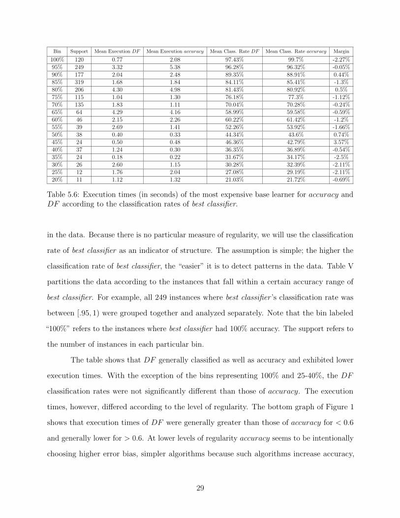
in the data. Because there is no particular measure of regularity, we will use the classification

rate of best classifier as an indicator of structure. The assumption is simple; the higher the

classification rate of best classifier, the “easier” it is to detect patterns in the data. Table V

partitions the data according to the instances that fall within a certain accuracy range of

best classifier. For example, all 249 instances where best classifier ’s classification rate was

between [.95, 1) were grouped together and analyzed separately. Note that the bin labeled

“100%” refers to the instances where best classifier had 100% accuracy. The support refers to

the number of instances in each particular bin.

The table shows that DF generally classified as well as accuracy and exhibited lower

execution times. With the exception of the bins representing 100% and 25-40%, the DF

classification rates were not significantly different than those of accuracy. The execution

times, however, differed according to the level of regularity. The bottom graph of Figure 1

shows that execution times of DF were generally greater than those of accuracy for < 0.6

and generally lower for > 0.6. At lower levels of regularity accuracy seems to be intentionally

choosing higher error bias, simpler algorithms because such algorithms increase accuracy,

29

0.2 0.4 0.6 0.8 1

0.2

0.4

0.6

0.8

1

Classification Rate for best classifierC

lass

ifica

tion

Rat

e DFaccuracy

0.2 0.4 0.6 0.8 10

2

4

Classification Rate for best classifier

Ave

rage

Exec

uti

onT

ime

(Sec

onds)

DFaccuracy

Figure 5.6: Classification rates and execution times (most expensive base learner) ofVoting(DF ) and Voting(accuracy) according to classification rates of best classifier

while DF is leaning towards relatively lower error bias, more expensive algorithms. This

occurs with DF because it has the latitude to choose less accurate algorithms as long as

there is enough diversity in the ensemble such that the number of instances in N10 and N01

is significantly higher than those in N00. These results suggest that for datasets that tend

towards lower classification rates, there is computational savings in using accuracy. However,

for more separable, regular datasets it pays computationally to use DF .

We now consider how accuracy and DF perform against other circumstances. We will

continue to restrict our analysis to Voting(accuracy) and Voting(DF ). When considering

accuracy, we will compare performance to two ensembles that represent the lower and upper

bounds of classification. The lower bound will be represented by Voting(random). This is

30

0 100 200 300 400 500 600 700

0.7

0.8

0.9

1

Number of Instances

Cla

ssifi

cati

onR

ate

DF

accuracy

best ensemble

random

0 100 200 300 400 500 600 7000

2

4

6

8

Number of Instances

Ave

rage

Exec

uti

onT

ime

(Sec

onds)

DFaccuracy

Figure 5.7: Classification rates and execution times (most expensive base learner) ofVoting(DF ) and Voting(accuracy) according to number of instances

the baseline that any useful method should clear. For the upper bound, we will show the

results of whichever method was most accurate for a given instance; which we will call best

ensemble. Figures 2-5 show how Voting(DF ) and Voting(accuracy) perform according to the

number of instances, features, classes, and base learners in common, respectively.

Figure 2 bins the instance by number of instances in the dataset being considered.

There appears to be little separation in classification rates between DF and accuracy when

binning by instances. They both are very close to, and sometimes represent, the best ensemble

for each bin. However, for higher number of instances, accuracy generally has higher execution

times. This can be explained by accuracy gravitating towards higher error bias learners when

31

0 20 40 60 80 100

0.4

0.6

0.8

Number of Features

Cla

ssifi

cati

onR

ate

DF

accuracy

best ensemble

random

0 20 40 60 80 100

0

10

20

30

Number of Features

Ave

rage

Exec

uti

onT

ime

(Sec

onds)

DFaccuracy

Figure 5.8: Classification rates and execution times (most expensive base learner) ofVoting(DF ) and Voting(accuracy) according to number of features

given more data and relying on lower error bias learners when the datasets are small. The

execution times of DF experience volatility, but do not increase by nearly as much as those

of accuracy as the number of instances increase.

Figures 3 and 4 show performance by number of features and number of classes,

respectively. We only note that the classification rates for accuracy and DF never significantly

differ. It is difficult to draw any conclusions from the execution times. The execution times

overall increase (almost exponentially), as would be expected, with an increase in the number

of classes and features.

32

0 5 10 15 20 25 300.4

0.6

0.8

Number of Classes

Cla

ssifi

cati

onR

ate

DF

accuracy

best ensemble

random

0 5 10 15 20 25 30

0

10

20

30

Number of Classes

Ave

rage

Exec

uti

onT

ime

(Sec

onds)

DFaccuracy

Figure 5.9: Classification rates and execution times (most expensive base learner) ofVoting(DF ) and Voting(accuracy) according to number of classes

33

0 1 2 3 4 5

0.7

0.8

0.9

Number of Base Learners in Common

Cla

ssifi

cati

onR

ate

DF

accuracy

best ensemble

random

0 1 2 3 4 5

0

5

10

15

Number of Base Learners in Common

Ave

rage

Exec

uti

onT

ime

(Sec

onds)

DFaccuracy

Figure 5.10: Classification rates and execution times (most expensive base learner) ofVoting(DF ) and Voting(accuracy) according to number of learners in common

34

Finally, Figure 5 shows an interesting result in which there is a distinct pattern in

classification rates and execution times with respect to the number of learners they have in

common. It appears that the classification rates are highest when accuracy and DF either

have no learners in common or all learners in common. A closer look reveals that the case

where DF and accuracy have all learners in common occurred in only 9 instances. Due to the

small sample size, we will ignore the case of total overlap for DF and accuracy and note that

the classification rate decreases somewhat monotonically with the number of base learners in

common. One explanation is that simpler datasets can be classified by most any classifier.

This leads to many ensembles having relatively similar DF scores. This wide diversity of

ensembles with low DF scores increases the probability that there will be little or no overlap

with ensembles optimized for accuracy. However, as datasets become less linearly separable,

a given learner’s error bias increasingly affects its classification rate, leading to disparity in

the accuracy of the available base learners. There will be fewer base learners to choose from

and the intersection between the accuracy and DF ensembles will grow.

We mentioned in the introduction that the voted ensemble would seem to favor accuracy

over diversity and that stacking was not as unfavorable towards diversity. The results bore

out these notions. Table III shows that the ensemble with the highest average accuracy was

Voted(accuracy). On the other hand, the least accurate ensemble was Voted(COD); with a

rate of 65.03%. Interestingly, the stacking algorithms were able to produce classification rates

of 5.26%, 5.80%, and 5.90% when optimized with COD. (Results not shown in Table III.)

The two measures introduced, sorted and composite, did not perform as well as DF

and accuracy in terms of classification rates. However, three of the ensembles based on

these measures (Stacking(sorted, bayes), Voting(sorted), and Stacking(composite, bayes)) did

outperform the best individual classifier, all random ensembles and all ensembles optimized

for DM,H and COD in Table III. In addition, the run times for sorted were lower than

those of DF and accuracy, while composite ensembles had runtimes about 3 times as fast as

those for accuracy.

35

Chapter 6

Conclusions

Three conclusions are readily drawn from the metadataset:

1. The region of the diversity space N11 is most critical for optimizing the accuracy of an

ensemble while the regions N10 and N01 are most critical for infusing diversity that

maintains relative accuracy. Directly optimizing levels of these three regions as opposed

to combining them with elements of N00 results in accurate, efficient ensembles.

2. A less obvious benefit of diversity is that it moves away from computationally expensive

learners and remains comparable to an ensemble optimized for accuracy. This has the

two-fold benefit of being accurate and less expensive than accuracy.

3. In the special case of datasets that do not exhibit regularity, ensembles optimized for

accuracy are more efficient. The more diverse ensembles simply model noise in different

ways and do not lead to a coherent metadataset in the case of stacking or a structured

consensus in the case of voting.

The first conclusion encourages researchers to combine N11, N10, and N01 in novel ways to

optimize both accuracy and efficiency. The last two conclusions encourage practitioners to

implement a measure based on the regularity of their data.

6.1 Future work

One aspect that was not explored here was concept drift. Intuition would suggest that the

diversity measures would perform better with respect to accuracy given that diverse ensembles

generalize better to new and changing data. Essentially, accuracy would be overfitting data.

36

We mentioned above the phenomenon of ensemble classification rates starting to

converge as the number of learners in the ensemble increases. It would be interesting to

analyze whether overall accuracy increases as the number of classifiers increases and whether

there is added computational expense in running more base learners in parallel. It is also

worth testing the performance of ensembles where the uniqueness of the learners is relaxed.

This would allow for ensembles to have more than one of a specific learner. This would

effectively give a duplicated learner more weight.

Future work could also involve modifying composite. While our study used α = 0.5,

we could assess the value of adjusting parameter α for the measure

αvoted(A,D) + (1− α)DF (A)

for voted ensembles and

αstacking(A,D) + (1− α)DF (A)

for stacking ensembles in order to optimize the resulting classification rates.

One could also substitute DF for COD in the above-mentioned formulas for composite.

Given that DF and accuracy are not metrics by definition, we cannot automatically assume

that triangular inequality applies to them. Hence, one may be tempted to think that a linear

combination of the two measures may result in performance better than DF or accuracy

individually. However, it is unlikely that such a composite would significantly outperform

DF or accuracy; if it is able to outperform them at all. In addition, there would be a

steep computational cost in substituting DF for COD. (See Table IV) In parametrizing

COD, we leave open the possibility that it can help the classification rate of composite

while maintaining the safeguard that it will be zeroed out if it is unhelpful. In either case,

composite will have a faster running time with COD and will not have a classification rate

significantly lower that if it were to include DF .

The sorted algorithm also has a parameter k that could be optimized. We used

k = 1000, which is a tiny fraction of the 1.2M available combinations of ensembles. Larger

values of k, such as 10,000-100,000 should be considered.

37

One last fine tuning of our study could include analysis of ECa. This measure takes

DF a step further by minimizing instances of pairwise learners agreeing on a misclassification.

Becasue it assigns the same value to N00D as to N11, N10, and N01, it is doubtful that the

measure would improve accuracy. It may, however, improve accuracy for the case of concept

drift in that it is slightly more diverse than DF .

38

References

[1] Thomas G. Dietterich. Ensemble methods in machine learning. Multiple classifier

systems, pages 1–15, 2000.

[2] Eugeniusz Gatnar. A diversity measure for tree-based classifier ensembles. Data Analysis

and Decision Support, pages 30–38, 2005.

[3] Giorgio Giacinto and Fabio Roli. Design of effective neural network ensembles for image

classification purposes. Image and Vision Computing, 19(9):699–707, 2001.

[4] Ludmila I. Kuncheva and Christopher J. Whitaker. Measures of diversity in classifier

ensembles and their relationship with the ensemble accuracy. Machine learning, 51(2):

181–207, 2003.

[5] Jun Won Lee and Christophe Giraud-Carrier. A metric for unsupervised metalearning.

Intelligent Data Analysis, 15(6):827–841, 2011.

[6] Adam H. Peterson and Tony R. Martinez. Estimating the potential for combining

learning models. pages 68–75, 2005.

[7] George Rudolph and Tony R. Martinez. Finding the real differences between learning

algorithms. International Journal on Artificial Intelligence Tools, 24(3):1550001, 2015.

[8] David B. Skalak. The sources of increased accuracy for two proposed boosting algorithms.

Proc. American Association for Artificial Intelligence, AAAI-96, Integrating Multiple

Learned Models Workshop, 1129:1133, 1996.

[9] David H. Wolpert. Stacked generalization. Neural networks, 5(2):241–259, 1992.

[10] G. Udny Yule. Notes on the theory of association of attributes in statistics. Biometrika,

2(2):121–134, 1903.

39

Appendix A

Visual Representation of Relationship Between Accuracy and Diversity

The following is a visual representation of relationship between accuracy and diversity.

We refer to the excellent graphical depiction put forth by Dietterich [1] found in Figure

6 to illustrate the principle. The figure shows a hypothesis space H, three different true

hypotheses f , and various learners h1, h2, .... Ensembles generally better approximate the

signal f by spanning a larger space than individual classifiers. Specifically, the upper left

depiction of H shows how the classifiers can combine their outputs and thereby reduce the

risk of misclassifying f . The upper right depiction of H depicts the computational savings of

ensemble methods. Each learner h1, h2, h3 may be able to accurately depict f given enough

training and tuning. However, the learners can reach a state similar to learners in the

Statistical example with much less training, thereby reducing the computational expense of

the ensemble. The example of H labeled Representational is similar to that of the figure

labeled Statistical except that in this case the learners are not able to model f individually.

However, they can be combined to model f .

Our result shows that diverse, inferior learners are able to span a space that is just as

effective for modeling f as the space spanned by an ensemble of accurate learners. Consider

Figures 7 & 8. The accurate learners in Figure 7 are able to individually approximate f to a

considerable degree. The learners in Figure 8 do not individually approximate f as well as

those in Figure 7. However, their outputs can be combined to produce a result comparable

to the combination of the learners in Figure 7. In the process, observe that the individual

diverse learners did not have to search H as much as the accurate learners. Hence, their

runtimes are lower.

40

Figure A.1: A graphical depiction of how the spaces spanned by ensembles better approximatethe signal f than the individual classifiers. Figure taken from [1].

Figure A.2: The accurate learners effectively approximate the true hypotheses f , but aftermuch training and fine-tuning.

Figure A.3: The diverse learners do not approximate f as well as the accurate learners, buttheir average approximates the function comparable to the accurate learners.

41

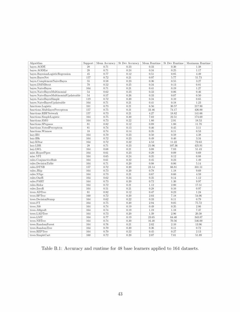
Appendix B

Results of Selected Algorithms Applied to 164 Datasets

Table VI shows the results of a pre-trial pass in which all available algorithms were

applied to the datasets that served as compatible inputs. In some cases, the feature type

was not compatible with a specified algorithm. weka implementations were used in all cases.

(See http://www.cs.waikato.ac.nz/ml/weka.)

42

Algorithm Support Mean Accuracy St Dev Accuracy Mean Runtime St Dev Runtime Maximum Runtimebayes.AODE 28 0.71 0.23 0.33 0.30 1.38bayes.AODEsr 28 0.71 0.24 0.34 0.25 1.17bayes.BayesianLogisticRegression 45 0.77 0.12 0.51 0.85 4.49bayes.BayesNet 157 0.72 0.21 0.97 5.77 51.73bayes.ComplementNaiveBayes 55 0.58 0.23 0.36 0.55 3.27bayes.DMNBtext 70 0.52 0.25 0.34 0.13 0.81bayes.NaiveBayes 164 0.71 0.21 0.41 0.19 1.27bayes.NaiveBayesMultinomial 54 0.62 0.23 0.33 0.06 0.46bayes.NaiveBayesMultinomialUpdateable 54 0.57 0.26 0.33 0.07 0.50bayes.NaiveBayesSimple 119 0.72 0.20 0.34 0.10 0.65bayes.NaiveBayesUpdateable 164 0.71 0.21 0.41 0.18 1.23functions.Logistic 161 0.73 0.21 6.56 30.57 217.90functions.MultilayerPerceptron 157 0.75 0.21 33.46 74.17 426.00functions.RBFNetwork 157 0.73 0.21 4.27 18.82 141.66functions.SimpleLogistic 164 0.75 0.20 7.02 22.51 174.69functions.SMO 164 0.73 0.22 1.80 2.91 18.53functions.SPegasos 81 0.82 0.12 0.89 1.80 11.78functions.VotedPerceptron 81 0.74 0.13 0.46 0.45 3.11functions.Winnow 18 0.74 0.14 0.35 0.11 0.53lazy.IB1 164 0.70 0.23 0.50 0.59 4.38lazy.IBk 164 0.72 0.23 0.49 0.40 3.34lazy.KStar 164 0.72 0.22 4.53 11.22 72.63lazy.LBR 28 0.71 0.23 21.06 107.36 425.91lazy.LWL 164 0.68 0.21 3.08 7.83 51.43misc.HyperPipes 164 0.61 0.23 0.29 0.09 0.69misc.VFI 164 0.65 0.24 0.35 0.12 0.88rules.ConjunctiveRule 164 0.61 0.22 0.45 0.23 1.49rules.DecisionTable 164 0.71 0.20 0.98 0.86 5.14rules.DTNB 157 0.72 0.20 23.14 66.81 331.51rules.JRip 164 0.73 0.20 0.78 1.18 9.69rules.NNge 164 0.73 0.21 0.67 0.60 4.59rules.OneR 164 0.62 0.24 0.35 0.14 1.12rules.PART 164 0.73 0.20 0.72 1.30 9.97rules.Ridor 164 0.72 0.21 1.12 2.80 17.51rules.ZeroR 164 0.51 0.21 0.28 0.10 0.97trees.ADTree 81 0.82 0.12 0.47 0.23 1.24trees.BFTree 160 0.72 0.20 2.03 7.18 54.96trees.DecisionStump 164 0.62 0.22 0.33 0.11 0.79trees.FT 164 0.75 0.20 2.94 9.05 75.72trees.J48 164 0.74 0.19 0.49 0.35 2.86trees.J48graft 164 0.74 0.19 1.19 1.18 7.37trees.LADTree 164 0.73 0.20 1.39 2.96 20.38trees.LMT 164 0.77 0.19 23.65 64.40 343.87trees.NBTree 164 0.74 0.20 16.48 70.56 546.00trees.RandomForest 164 0.76 0.21 2.02 2.10 13.96trees.RandomTree 164 0.70 0.20 0.36 0.11 0.72trees.REPTree 164 0.70 0.22 0.45 0.27 2.13trees.SimpleCart 160 0.72 0.20 2.07 7.01 51.89

Table B.1: Accuracy and runtime for 48 base learners applied to 164 datasets.

43