DISTRIBUTIONS IN FINANCIAL MATHEMATICS … material is based on the synthesis of several lecture...
67
University of Tartu Faculty of Mathematics and Computer Science Institute of Mathematical Statistics DISTRIBUTIONS IN FINANCIAL MATHEMATICS (MTMS.02.023) Lecture notes Ants Kaasik, Meelis K¨ a¨ arik
-
Upload
nguyenlien -
Category
Documents
-
view
216 -
download
2
Transcript of DISTRIBUTIONS IN FINANCIAL MATHEMATICS … material is based on the synthesis of several lecture...

University of Tartu
Faculty of Mathematics and Computer Science
Institute of Mathematical Statistics
DISTRIBUTIONS IN FINANCIAL
MATHEMATICS (MTMS.02.023)
Lecture notes
Ants Kaasik, Meelis Kaarik

MTMS.02.023. Distributions in Financial Mathematics
Contents
1 Introduction 1
1.1 The data. Prediction problem . . . . . . . . . . . . . . . . . . 1
1.2 The models . . . . . . . . . . . . . . . . . . . . . . . . . . . . 2
1.3 Summary of the introduction . . . . . . . . . . . . . . . . . . 2
2 Exploration and visualization of the data 2
2.1 Motivating example . . . . . . . . . . . . . . . . . . . . . . . 2
3 Heavy-tailed probability distributions 7
4 Detecting the heaviness of the tail 10
4.1 Visual tests . . . . . . . . . . . . . . . . . . . . . . . . . . . . 10
4.2 Maximum-sum ratio test . . . . . . . . . . . . . . . . . . . . . 13
4.3 Records test . . . . . . . . . . . . . . . . . . . . . . . . . . . . 14
4.4 Alternative definition of heavy tails . . . . . . . . . . . . . . . 15
5 Creating new probability distributions. Mixture distribu-tions 17
5.1 Combining distributions. Discrete mixtures . . . . . . . . . . 17
5.2 Continuous mixtures . . . . . . . . . . . . . . . . . . . . . . . 19
5.3 Completely new parts . . . . . . . . . . . . . . . . . . . . . . 20
5.4 Parameters of a distribution . . . . . . . . . . . . . . . . . . . 21
6 Empirical distribution. Kernel density estimation 22
7 Subexponential distributions 27
7.1 Preliminaries. Definition . . . . . . . . . . . . . . . . . . . . . 27
7.2 Properties of subexponential class . . . . . . . . . . . . . . . 28
8 Well-known distributions in financial and insurance mathe-matics 30
8.1 Exponential distribution . . . . . . . . . . . . . . . . . . . . . 30
8.2 Pareto distribution . . . . . . . . . . . . . . . . . . . . . . . . 31
8.3 Weibull Distribution . . . . . . . . . . . . . . . . . . . . . . . 33
i
MTMS.02.023. Distributions in Financial Mathematics
8.4 Lognormal distribution . . . . . . . . . . . . . . . . . . . . . . 34
8.5 Log-gamma distribution . . . . . . . . . . . . . . . . . . . . . 35
8.6 Burr distribution . . . . . . . . . . . . . . . . . . . . . . . . . 36
9 Introduction to the extreme value theory (EVT) 38
9.1 Preliminaries. Max-stable distributions . . . . . . . . . . . . . 38
9.2 Forms of max-stable distributions . . . . . . . . . . . . . . . . 40
9.3 Extreme value theorem. Examples . . . . . . . . . . . . . . . 42
9.4 Generalized extreme value distribution . . . . . . . . . . . . . 45
9.5 Generalized Pareto distribution (GPD) . . . . . . . . . . . . . 48
10 Stable distributions 51
11 Geometric stable distributions 55
12 Goodness of fit of a model 59
12.1 Kolmogorov-Smirnov test . . . . . . . . . . . . . . . . . . . . 59
12.2 Anderson-Darling test . . . . . . . . . . . . . . . . . . . . . . 61
12.3 Likelihood ratio test . . . . . . . . . . . . . . . . . . . . . . . 61
12.4 Information criteria. Akaike information criterion (AIC) . . . 62
13 Conclusion 63
ii
MTMS.02.023. Distributions in Financial Mathematics
Course material is based on the synthesis of several lecture notes about prob-ability distributions and books that are available in the university library.This material includes most important aspects of the course but reading itis by no means equal to the experience that is gained in the lecture.
Some key textbooks:Klugman, Panjer & Willmot (2004). Loss Models: From Data to Decisions.Cooke & Nieboer (2011). Heavy-Tailed Distributions: Data, Diagnostics, andNew Developments.Balakrishnan, Nevzorov (2003). A Primer on Statistical Distributions.Evans, Hastings & Peacock (2000). Statistical Distributions.Embrechts, Mikosch & Kluppelberg (1997). Modelling Extremal Events: forInsurance and Finance.Resnick (2007). Heavy-Tail Phenomena: Probabilistic and Statistical Model-ing
1 Introduction
1.1 The data. Prediction problem
In many applications of the financial mathematics we want to look at thefuture (i.e. predict what are the possible scenarios and how likely they are).But this can only be based on the past (and present). So we train a model(estimate model parameters) using available data (training data). But it istypically not the model that we are interested in, rather we have a practicalquestion that needs answering (”how probable is it that the investment willnot return the required 5%”). However, to answer this question a modelis still typically needed and when this is postulated (and the parametersestimated) then answering the initial question is straightforward.
So the first question is how the data is generated (what is the model respon-sible)? Usually this means that we pick a parametric model and estimatethe model parameters using the training data. This seems reasonable butunfortunately reality is (typically) different – we are lucky if the model fitsthe data well but it is very unlikely that the model is true (if we do notconsider simple physical experiments like die casting or measurement errordistribution). Still, this approach might be the best we can (or are able to)do.
What is also important to remember: observations are typically not inde-pendent but if we must make this assumption then we must do our best sothat the assumption would be violated by (our transformed) data ”as littleas possible”. For example, it is very hard believe that stock prices (for a
1
MTMS.02.023. Distributions in Financial Mathematics
particular stock) for successive days are independent, but changes in priceare more likely to be.
1.2 The models
Let us consider some data (say, 100 observations) and think of the firstmodel that crosses your mind? With financial data it is likely that simplemodels are not very realistic. At least not in the long run. This is probablyso but we can also consider that the model parameters are time dependent(i.e. not constant in time) or a change to a different distribution occurs. AHidden Markov Model (HMM) is already complex enough to be plausible.But even for this complex model any given observation is still a realizationfrom some (univariate) probability distribution. So to be able to use thismodel we definitely need to know the possible candidates for univariatedistributions. This is the reason why we consider (nothing but) univariateprobability distributions in the course.
Of course if we are interested e.g. in a quantile only (and we have plentyof data) then it might be possible to not make an assumption of a specificunderlying parametric distribution as we are not interested in it.
On rare occasions we might in fact find a theoretically justified distributionmodel (as is the case with die casting) Central Limit Theorem (CLT) is themost prominent example.
1.3 Summary of the introduction
We will use real data to study the particularities of the data that arises infinancial mathematics and also consider how to use those particularities. Todo this we need additional notations. This makes it easier to classify prob-ability distributions. We consider different distributions that are possiblemodels for financial data. We also consider the distribution free approach(which is based on either the empirical cumulative distribution function (cdf)or empirical probability density function (pdf)). Some attention is given tothe practical ways of picking a suitable model (out of a list of candidatemodels).
2 Exploration and visualization of the data
2.1 Motivating example
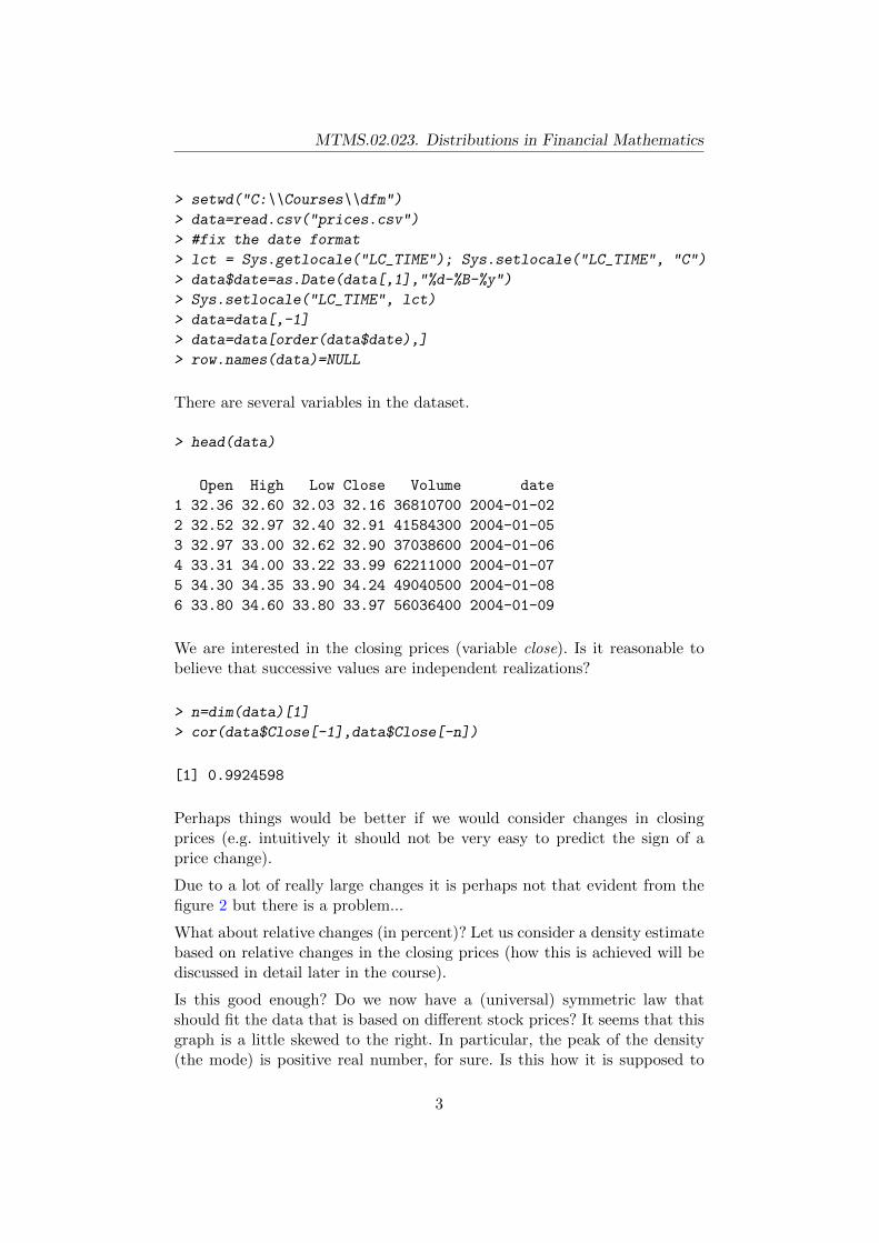
Consider these (real) stock prices spanning 5 years (file prices.csv).
2
MTMS.02.023. Distributions in Financial Mathematics
> setwd("C:\\Courses\\dfm")
> data=read.csv("prices.csv")
> #fix the date format
> lct = Sys.getlocale("LC_TIME"); Sys.setlocale("LC_TIME", "C")
> data$date=as.Date(data[,1],"%d-%B-%y")
> Sys.setlocale("LC_TIME", lct)
> data=data[,-1]
> data=data[order(data$date),]
> row.names(data)=NULL
There are several variables in the dataset.
> head(data)
Open High Low Close Volume date
1 32.36 32.60 32.03 32.16 36810700 2004-01-02
2 32.52 32.97 32.40 32.91 41584300 2004-01-05
3 32.97 33.00 32.62 32.90 37038600 2004-01-06
4 33.31 34.00 33.22 33.99 62211000 2004-01-07
5 34.30 34.35 33.90 34.24 49040500 2004-01-08
6 33.80 34.60 33.80 33.97 56036400 2004-01-09
We are interested in the closing prices (variable close). Is it reasonable tobelieve that successive values are independent realizations?
> n=dim(data)[1]
> cor(data$Close[-1],data$Close[-n])
[1] 0.9924598
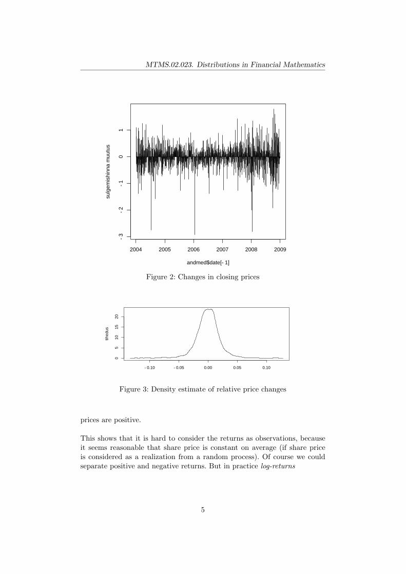
Perhaps things would be better if we would consider changes in closingprices (e.g. intuitively it should not be very easy to predict the sign of aprice change).
Due to a lot of really large changes it is perhaps not that evident from thefigure 2 but there is a problem...
What about relative changes (in percent)? Let us consider a density estimatebased on relative changes in the closing prices (how this is achieved will bediscussed in detail later in the course).
Is this good enough? Do we now have a (universal) symmetric law thatshould fit the data that is based on different stock prices? It seems that thisgraph is a little skewed to the right. In particular, the peak of the density(the mode) is positive real number, for sure. Is this how it is supposed to
3

MTMS.02.023. Distributions in Financial Mathematics
2004 2005 2006 2007 2008 2009
1520
2530
35
andmed$date
sulg
emis
hind
Figure 1: Closing prices
be? Perhaps it is just because the stock price has increased in the long run?Let us look at the figure 1 again.
Perhaps this asymmetric distribution can be explained with the fact thatthere are simply more large declines and to compensate many small increasesare required. This is partly true in this case. But let us pause for a moment.Suppose the closing price on the first day is 100, on the second day it is 110and on the third day it is 100 again. So the price has not actually changedover 2 days.But what about the returns or relative changes in price? For thefirst change it is 0.1 or ten percent but it is not −0.1 for the second change,because for this the drop must have been 11 units. Thus something closer tozero (−1/11 to be more precise). So the initial and final price are the samebut we got two returns which both have different sign but the positive oneis larger in absolute value. Is this a coincidence?
Home assignment 1. Show that for equal initial and final price (pt =pt+2) and some different price in between (pt+1 6= pt) we get two returns(pt+2− pt+1)/pt+1 and (pt+1− pt)/pt such that the positive return is alwayslarger in absolute value. Show that it is not important whether the priceincreases (pt+1 > pt) or decreases (pt+1 < pt) at first. We consider that all
4
MTMS.02.023. Distributions in Financial Mathematics
2004 2005 2006 2007 2008 2009
−3
−2
−1
01
andmed$date[−1]
sulg
emis
hinn
a m
uutu
s
Figure 2: Changes in closing prices
−0.10 −0.05 0.00 0.05 0.10
05
1015
20
tihed
us
Figure 3: Density estimate of relative price changes
prices are positive.
This shows that it is hard to consider the returns as observations, becauseit seems reasonable that share price is constant on average (if share priceis considered as a realization from a random process). Of course we couldseparate positive and negative returns. But in practice log-returns
5
MTMS.02.023. Distributions in Financial Mathematics
lnpt+1
pt,
are considered instead. It is easy to see that if pt = pt+2 then ln(pt+1/pt)are ln(pt+2/pt+1) equal in absolute value. Also, log-returns are very close toreturns because
ln(1 + x) =∞∑n=1
(−1)n+1xn
n, if − 1 < x 6 1.
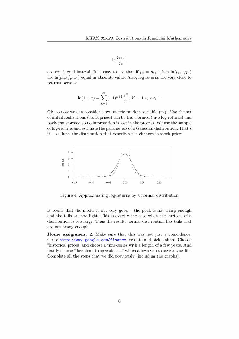
Ok, so now we can consider a symmetric random variable (rv). Also the setof initial realizations (stock prices) can be transformed (into log-returns) andback-transformed so no information is lost in the process. We use the sampleof log-returns and estimate the parameters of a Gaussian distribution. That’sit – we have the distribution that describes the changes in stock prices.
−0.15 −0.10 −0.05 0.00 0.05 0.10
05
1015
20
tihed
us
Figure 4: Approximating log-returns by a normal distribution
It seems that the model is not very good – the peak is not sharp enoughand the tails are too light. This is exactly the case when the kurtosis of adistribution is too large. Thus the result: normal distribution has tails thatare not heavy enough.
Home assignment 2. Make sure that this was not just a coincidence.Go to http://www.google.com/finance for data and pick a share. Choose”historical prices” and choose a time-series with a length of a few years. Andfinally choose ”download to spreadsheet” which allows you to save a .csv -file.Complete all the steps that we did previously (including the graphs).
6
MTMS.02.023. Distributions in Financial Mathematics
3 Heavy-tailed probability distributions
What could we choose as a distribution model? What distribution has a tailwhich is heavier than that of a normal (Gaussian) distribution. What aboutt-distribution?
Home assignment 3. Read R help for the function dt (i.e. the density func-tion of a t-distribution) and pay attention how the variance is expressed. Usethe data from the previous (log-returns) and estimate the variance. Explainwhy the method of moments cannot be used for fitting the distribution (wecan make a simplification and say that the expectation is zero, then a singleequation is needed).
Now, one of the models has a tail that is too light and another one has atail that is too heavy. Thus, it would be nice to have something that wouldallow us to compare distributions based on their respective tails. Perhapsthe easiest approach would be a comparison of two distributions.
Let us consider two probability density functions f1(x) and f2(x), respec-tively, and we compare their right tails (for simplicity assume that ∃K ∈ R :∀x > K f1(x) > 0, f2(x) > 0).
Definition 3.1. If it holds that
limx→∞
f1(x)
f2(x)=∞,
then we say that the distribution corresponding to probability density func-tion f1(x) has a heavier tail than the distribution corresponding to probabilitydensity function f2(x).
The definition for comparing left tails is similar.
Home assignment 4. Which distribution out of the three has the lightesttail and which one has the heaviest? Explain your answer!
1. f1(x) = αθα
(x+θ)α+1 , α > 0, θ > 0, x > 0,
2. f2(x) = 1xσ√
2πe−
(ln x−µ)2
2σ2 , µ ∈ R, σ > 0, x > 0,
3. f3(x) = kλ
(xλ
)k−1e−( xλ)
k
, λ > 0, k > 0, x > 0.
To simplify, it is allowed to fix θ = 1, µ = 0, σ = 1/√
2 and λ = 1.
Now we can fix some distribution F and say what distributions have a lighterand which ones a heavier tail than F . We could call the former light-taileddistributions and the latter heavy-tailed distributions. We consider threeadditional functions that help us describe a distribution.
7
MTMS.02.023. Distributions in Financial Mathematics
Definition 3.2. Tail distribution function (also known as survival function)of a random variable X with cumulative distribution function F (x) is thefunction
F (x) = 1− F (x) = P(X > x).
By definition this is a non-increasing function that is left-continuous.
Intuitive way of comparing distributions would be to consider F1(x) andF2(x).
Definition 3.3. If
limx→∞
F1(x)
F2(x)=∞,
then we say that the distribution corresponding to F1(x) has a heavier tailthan the distribution corresponding to F2(x).
L’Hospital rule allows us to conclude that this definition is actually equal tothe one given previously.
Definition 3.4. Hazard function (also known as instantaneous failure rate)of the random variable X is the function
h(x) =f(x)
F (x),
where f(x) is the probability density function of X and F (x) is the taildistribution function of X.
For a (continuous) random variable X the hazard function at x is thus theconditional density function of X at x under the condition that X > x.If the hazard function is a decreasing function then ”for large values theprobability of a particular value is decreasing and thus the probability oflarger values increasing”. This is characteristic to heavy-tailed distributions.If the hazard function is increasing then the tail of the distribution is light.This characterization places exponential distribution on the borderline – itshazard function is constant.
Definition 3.5. Mean excess function of a random variable X (also knownas mean residual life function) is the conditional expectation
e(x) = E(X − x|X > x).
Partial integration gives us
e(x) =
∫∞x (y − x)f(y)dy
F (x)=−(y − x)F (y)|∞x +
∫∞x F (y)dy
F (x)
=
∫∞x F (y)dy
F (x).
8

MTMS.02.023. Distributions in Financial Mathematics
If e(x) is increasing then ”the mean exceedance of a particular value is in-creasing for large values” and thus the random variable has a heavy tail. Adecreasing mean excess function corresponds to a light tail. Similarly withthe previous case the borderline distribution is exponential.
Home assignment 5. Prove that the mean excess function is constant forexponential distribution. Use the relationship between e(x) and F (x) thatwas discovered previously.
9

MTMS.02.023. Distributions in Financial Mathematics
4 Detecting the heaviness of the tail
4.1 Visual tests
Now we know that exponential distribution is on the borderline of light andheavy-tailed distributions. So perhaps it would be a good candidate for thelog-returns data (it has a heavier tail than a normal distribution as can easilybe seen when comparing the densities). Of course, exponential distributionhas positive support so we can only use positive log-returns (at first).
0.00 0.02 0.04 0.06 0.08 0.10 0.12
020
4060
80
tihed
us
Figure 5: Approximating the positive log-returns with an exponential distri-bution
The fit seems quite decent, at least as far as the tail is concerned. Histogramis a useful graph to visualize the fit (in addition to the densities). Seems thatthe data is not from the exponential distribution.
sage
dus
0.00 0.02 0.04 0.06 0.08 0.10 0.12
020
4060
80
Figure 6: Histogram of the positive log-returns
It is important to note that even though it seems that extreme values fromthe tail are very unlikely to realize (usually the value of a share does notdouble in a day, but it actually can happen) it can be very important topredict correctly the frequency of 10% gains. But our financial data can bealso of different nature (e.g. insurance claims) where the upper limit reallyis not clear (of course, the insurance can have a re-insurance contract butthe tail behaviour is just as important – e.g. deductible can be a percentageof the total cost)
10

MTMS.02.023. Distributions in Financial Mathematics
To compare the theoretical distribution with the data at hand we can alsomake use of a quantile-quantile graph (QQ-plot): one axis has the samplequantiles and the other the theoretical quantiles.
Consider an ordered sample (x(1), . . . , x(n)), i.e. x(1) ≤ . . . ≤ x(n) and let Hbe the theoretical candidate probability distribution function. Then we canplot {
x(i), H−1
(i
n+ 1
)}, i = 1, . . . , n.
Whether the theoretical quantiles are on the horizontal or vertical axis canvary but usually a line through the quartiles is plotted. It is important tonote that we are not concerned with the location and scale parameter –these do not change the shape of a graph. This is true because such a lineartransform does not change the order nor does it change how many timessome value is larger than the other. So we can instead imagine that we plot{
a+ bx(i), H−1
(i
n+ 1
)}, i = 1, . . . , n,
which only differs in scale.
0 1 2 3 4 5 6 7
0.00
0.04
0.08
teoreetilised kvantiilid
valim
i kva
ntiil
id
●●●●●●●●●●●●●●●●●●●●●●●●●●●●●●●●●●●●●●●●●●●●●●●●●●●●●●●●●●●●●●●●●●●●●●●●●●●●●●●●●●●●●●●●●●●●●●●●●●●●●●●●●●●●●●●●●●●●●●●●●●●●●●●●●●●●●●●●●●●●●●●●●●●●●●●●●●●●●●●●●●●●●●●●●
●●●●●●●●●●●●●●●●●●●●●●●●●●●●●●●●●●●●●●●●●●●●●●●●●●●●●●●●●●●●●●●●●●●●●●●●●●●●●●●●●●●●●●●●●●●●●●●●●●●●●●●●●●●●●●●●●●●●●●●●●●●●●●●●●●●●●●●●●●●●●●●●●●●●●●●●●●●●●●●●●●●●●●●●●●●●●●
●●●●●●●●●●●●●●●●●●●●●●●●●●●●●●●●●●●●●●●●●●●●●●●●●●●●●●●●●●●●●●●●●●●●●●●●●●●●●●●●●●●●●●●●●●●●●●●●●●●●●●●●●●●
●●●●●●●●●●●●●●●●●●●●●●●●●●●●●●●●●●●●●●●●●●●●●●●●●●●●●●●●●●●●●●●●●●●
●●●●●●●●●●●●●●●●●●●●●●●●●●●●●●●●●●●
●●●●●●●●●●●●●●●●●●●●●●●●●●●●
●●●●●●●●●●●●●●●
●●●●●●●●●●●●●●●●●●
●●
● ● ●
● ●
●●
Figure 7: QQ-plot of positive log-returns and the exponential distribution
Home assignment 6. When drawing a QQ-plot why is H−1(i/(n + 1))plotted instead of H−1(i/n)?
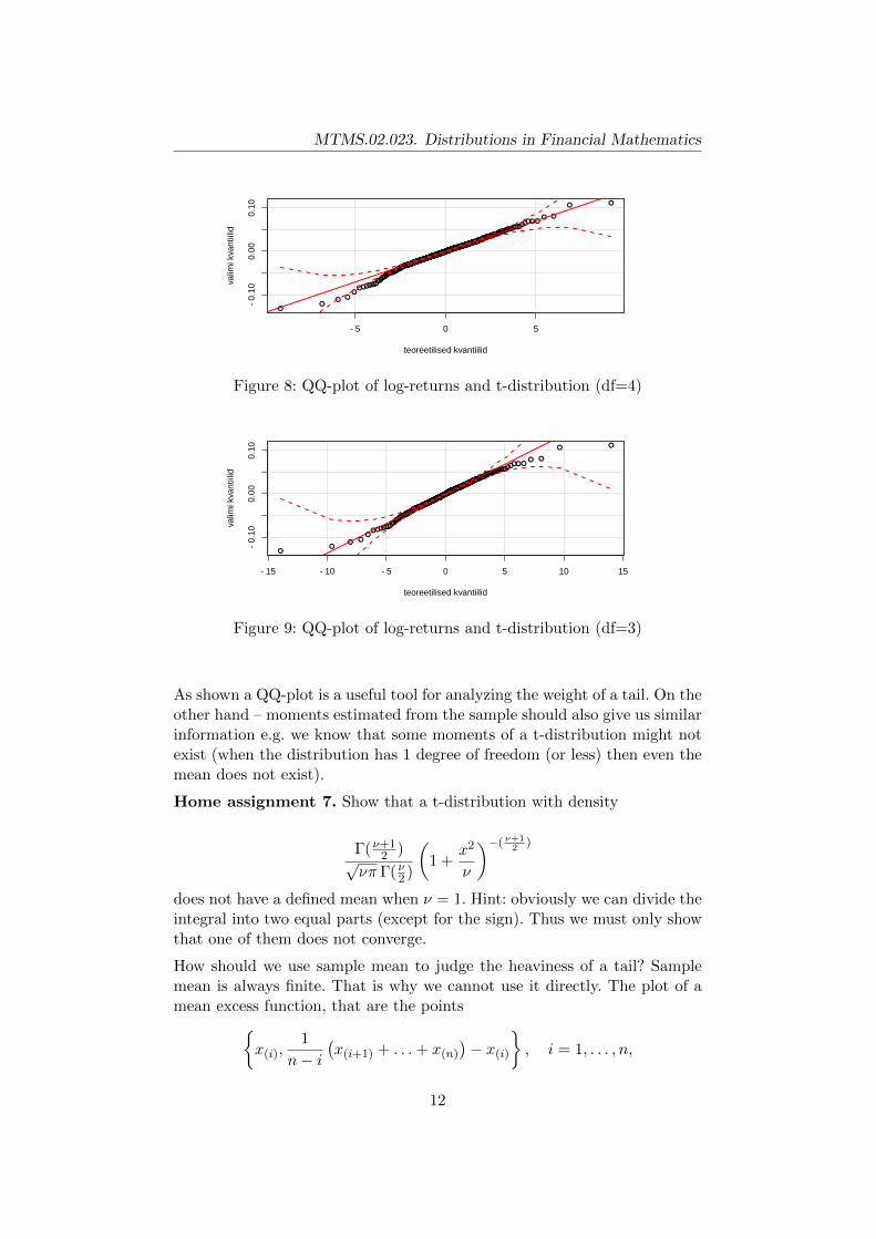
As we see from 7 declaring a good fit was a bit too hasty – several pointsare outside of the confidence intervals and the slopes seem different. To bemore precise: the tail of the exponential distribution is too light as it predictssmaller quantile values than they are in the actual sample. Figure 8 shows,that a t-distribution with 4 degrees of freedom fits the positive log-returndata well. For the negative returns such a tail seems to light and thus asmaller degrees of freedom should be used (this means a heavier tail fort-distribution).
11
MTMS.02.023. Distributions in Financial Mathematics
−5 0 5
−0.
100.
000.
10
teoreetilised kvantiilid
valim
i kva
ntiil
id
●●
● ●●
●●●●●●●●●●
●●●●●●●●●●●●
●●●●●●●●●●●●●●●●●●●●●
●●●●●●●●●●●●●●●●●●●●●●●●●●●●●●●●●●●●●●●●●●●●●●●●●●●●●●●●●●●●●●●●●●●●●●●●●
●●●●●●●●●●●●●●●●●●●●●●●●●●●●●●●●●●●●●●●●●●●●●●●●●●●●●●●●●●●●●●●●●●●●●●●●●●●●●●●●●●●●●●●●●●●●●●●●●●●●●●●●●●●●●●●●●●●●●●●●●●●●●●●●●●●●●●●●●●●●●●●●●●●●●●●●●●●●●●●●●●●●●●●●●●●●●●●●●●●●●●●●●●●●●●●●●●●
●●●●●●●●●●●●●●●●●●●●●●●●●●●●●●●●●●●●●●●●●●●●●●●●●●●●●●●●●●●●●●●●●●●●●●●●●●●●●●●●●●●●●●●●●●●●●●●●●●●●●●●●●●●●●●●●●●●●●●●●●●●●●●●●●●●●●●●●●●●●●●●●●●●●●●●●●●●●●●●●●●●●●●●●●●●●●●●●●●●●●●●●●●●●●●●●●●●●●●●●●●●●●●●●●●●●●●●●●●●●●●●●●●●●●●●●●●●●●●●●●●●●●●●●●●●●●●●●●●●●●●●●●●●●●●●●●●●●●●●●●●●●●●●●●●●●●●●●●●●●●●●●●●●●●●●●●●●●●●●●●●●●●●●●●●●●●●●●●●●●●●●●●●●●●●●●●●●●●●●●●●●●●●●
●●●●●●●●●●●●●●●●●●●●●●●●●●●●●●●●●●●●●●●●●●●●●●●●●●●●●●●●●●●●●●●●●●●●●●●●●●●●●●●●●●●●●●●●●●●●●●●●●●●●●●●●●●●●●●●●●●●●●●●●●●●●●●●●●●●●●●●●●●●●●●●●●●●●●●●●●●●●●●●●●●●●●●●●●●●●●●●●●●●●●●●●●●●●●●●●●●●●●●●●●●●●●●●●●●●●●●●●●●●●●●●●●●●●●●●●●●●●●●●●●●●●●●●●●●●●●●●●●●●●●●●●●●●●●●●●●●●●●●●●●●●●●●●●●●●●●●●●●●●●●●●●●●●●●●●●●●●●●●●●●●●●●●●●●●●●●●●●●●●●●●●●●●
●●●●●●●●●●●●●●●●●●●●●●●●●●●●●●●●●●●●●●●●●●●●●●●●●●●●●●●●●●●●●●●●●●●●●●●●●●●●●●●●●●●●●●●●●●●●●●●●●●●●●●●●●●●●●●●●●●●●●●●●●●●●●●●●●●●●●●●●●●●●●●●●●●●
●●●●●●●●●●●●●●●●●●●●●●●●●●●●●●●●●●●●●●●●●●●●●●●●●●
●●●●●●●●●●●●●●●●●●●
●●●●●●●●●●●
● ●
● ●
Figure 8: QQ-plot of log-returns and t-distribution (df=4)
−15 −10 −5 0 5 10 15
−0.
100.
000.
10
teoreetilised kvantiilid
valim
i kva
ntiil
id
●●
● ●●
●●●●●●●●●●
●●●●●●●●●●●●
●●●●●●●●●●●●●●●●●●●●●
●●●●●●●●●●●●●●●●●●●●●●●●●●●●●●●●●●●●●●●●●●●●●●●●●●●●●●●●●●●●●●●●●●●●●●●●●
●●●●●●●●●●●●●●●●●●●●●●●●●●●●●●●●●●●●●●●●●●●●●●●●●●●●●●●●●●●●●●●●●●●●●●●●●●●●●●●●●●●●●●●●●●●●●●●●●●●●●●●●●●●●●●●●●●●●●●●●●●●●●●●●●●●●●●●●●●●●●●●●●●●●●●●●●●●●●●●●●●●●●●●●●●●●●●●●●●●●●●●●●●●●●●●●●●●
●●●●●●●●●●●●●●●●●●●●●●●●●●●●●●●●●●●●●●●●●●●●●●●●●●●●●●●●●●●●●●●●●●●●●●●●●●●●●●●●●●●●●●●●●●●●●●●●●●●●●●●●●●●●●●●●●●●●●●●●●●●●●●●●●●●●●●●●●●●●●●●●●●●●●●●●●●●●●●●●●●●●●●●●●●●●●●●●●●●●●●●●●●●●●●●●●●●●●●●●●●●●●●●●●●●●●●●●●●●●●●●●●●●●●●●●●●●●●●●●●●●●●●●●●●●●●●●●●●●●●●●●●●●●●●●●●●●●●●●●●●●●●●●●●●●●●●●●●●●●●●●●●●●●●●●●●●●●●●●●●●●●●●●●●●●●●●●●●●●●●●●●●●●●●●●●●●●●●●●●●●●●●●●
●●●●●●●●●●●●●●●●●●●●●●●●●●●●●●●●●●●●●●●●●●●●●●●●●●●●●●●●●●●●●●●●●●●●●●●●●●●●●●●●●●●●●●●●●●●●●●●●●●●●●●●●●●●●●●●●●●●●●●●●●●●●●●●●●●●●●●●●●●●●●●●●●●●●●●●●●●●●●●●●●●●●●●●●●●●●●●●●●●●●●●●●●●●●●●●●●●●●●●●●●●●●●●●●●●●●●●●●●●●●●●●●●●●●●●●●●●●●●●●●●●●●●●●●●●●●●●●●●●●●●●●●●●●●●●●●●●●●●●●●●●●●●●●●●●●●●●●●●●●●●●●●●●●●●●●●●●●●●●●●●●●●●●●●●●●●●●●●●●●●●●●●●●
●●●●●●●●●●●●●●●●●●●●●●●●●●●●●●●●●●●●●●●●●●●●●●●●●●●●●●●●●●●●●●●●●●●●●●●●●●●●●●●●●●●●●●●●●●●●●●●●●●●●●●●●●●●●●●●●●●●●●●●●●●●●●●●●●●●●●●●●●●●●●●●●●●●
●●●●●●●●●●●●●●●●●●●●●●●●●●●●●●●●●●●●●●●●●●●●●●●●●●
●●●●●●●●●●●●●●●●●●●
●●●●●●●●●● ●
● ●
● ●
Figure 9: QQ-plot of log-returns and t-distribution (df=3)
As shown a QQ-plot is a useful tool for analyzing the weight of a tail. On theother hand – moments estimated from the sample should also give us similarinformation e.g. we know that some moments of a t-distribution might notexist (when the distribution has 1 degree of freedom (or less) then even themean does not exist).
Home assignment 7. Show that a t-distribution with density
Γ(ν+12 )
√νπ Γ(ν2 )
(1 +
x2
ν
)−( ν+12
)
does not have a defined mean when ν = 1. Hint: obviously we can divide theintegral into two equal parts (except for the sign). Thus we must only showthat one of them does not converge.
How should we use sample mean to judge the heaviness of a tail? Samplemean is always finite. That is why we cannot use it directly. The plot of amean excess function, that are the points{
x(i),1
n− i(x(i+1) + . . .+ x(n)
)− x(i)
}, i = 1, . . . , n,
12

MTMS.02.023. Distributions in Financial Mathematics
is an example. Figure 10 is for our positive log-returns, and it points at aheavy tail. However, very wide confidence intervals must be noted. This istypical because (however large the sample) as we move closer to the largevalues of the sample there will be little information left. Unfortunately thisis exactly the most interesting (/important) part of the figure.
0.00 0.01 0.02 0.03 0.04 0.05 0.06 0.07
0.00
00.
010
0.02
00.
030
lävend
kesk
min
e ül
etam
ine
Figure 10: Empirical mean excess function for the positive log-returns
Figure 11 illustrates a heavy tail (t-distribution with 1 degree of freedom)
0 10 20 30 40 50
050
150
250
350
lävend
kesk
min
e ül
etam
ine
Figure 11: A mean excess function based on a sample with size 1000 fromthe t-distribution (df=1)
4.2 Maximum-sum ratio test
When a heavy tail is suspected then the existence of moments is not guar-anteed. To test this for a sample (of positive values) the ratio between themaximum and the sum of a sample can be used.
Consider the ratioMn(p)/Sn(p), i = 1, . . . , n,
where
p > 0 and Sn(p) = Xp1 + . . .+Xp
n, Mn(p) = max{Xp1 , . . . , X
pn}.
13

MTMS.02.023. Distributions in Financial Mathematics
It holds that
P(Mn(p)
Sn(p)→ 0
)= 1⇔ E|X|p <∞.
As can be seen from figures 12 and 13 it is pretty easy to test this for somemoments (for our log-returns data) – mean is finite but the fifth momentprobably does not exist.
0 100 200 300 400 500 600
0.0
0.2
0.4
0.6
0.8
1.0
Figure 12: The ratio of maximum and sum for positive log-returns whenp = 1
0 100 200 300 400 500 600
0.0
0.2
0.4
0.6
0.8
1.0
Figure 13: The ratio of maximum and sum for positive log-returns whenp = 5
4.3 Records test
Before we analyzed the tail weight but what can be said about independenceof the sample elements? If our realizations are not independent (and this is ofcourse quite common for returns as clustering is common (bearish or bullishmarket)), it is useful to analyze the records.
In order to introduce the notion of records we need to bring in some addi-tional notation. Let us consider a sequence of random variables, X1, X2, . . .,
14
MTMS.02.023. Distributions in Financial Mathematics
and denote the maximum of first n random variables by Mn:
M1 = X1, Mn = maxi=1,...,n
(X1, . . . , Xn), n ≥ 2.
Definition 4.1. Records ri in sequence X1, X2, . . . are defined by:
• r1 = X1,
• ri = Xn if Xn > Mn−1 (where i is the record index).
In other words, a record is a temporary maximum in the sequence of Xn.
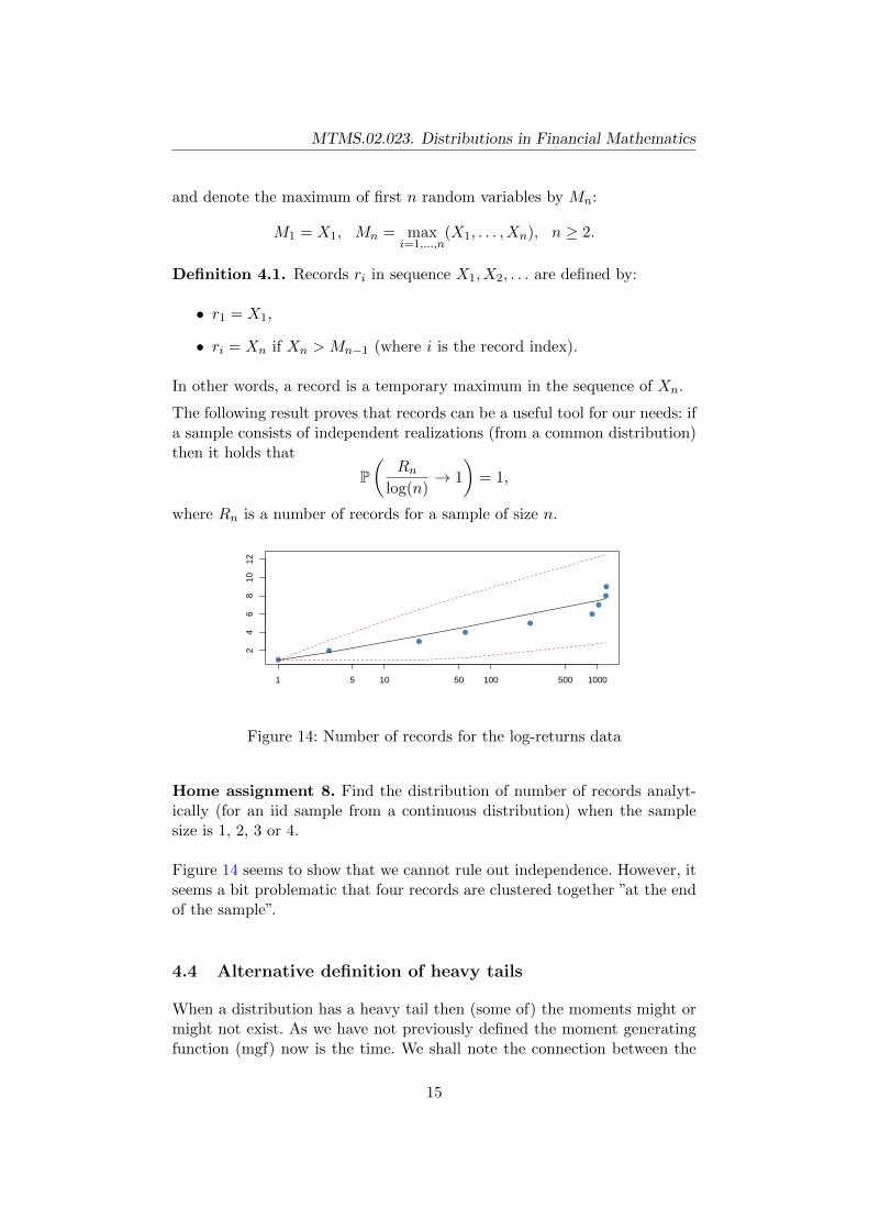
The following result proves that records can be a useful tool for our needs: ifa sample consists of independent realizations (from a common distribution)then it holds that
P(
Rnlog(n)
→ 1
)= 1,
where Rn is a number of records for a sample of size n.
●
●
●
●
●
●
●
●
●
1 5 10 50 100 500 1000
24
68
1012
Figure 14: Number of records for the log-returns data
Home assignment 8. Find the distribution of number of records analyt-ically (for an iid sample from a continuous distribution) when the samplesize is 1, 2, 3 or 4.
Figure 14 seems to show that we cannot rule out independence. However, itseems a bit problematic that four records are clustered together ”at the endof the sample”.
4.4 Alternative definition of heavy tails
When a distribution has a heavy tail then (some of) the moments might ormight not exist. As we have not previously defined the moment generatingfunction (mgf) now is the time. We shall note the connection between the
15

MTMS.02.023. Distributions in Financial Mathematics
existence of moments and the mgf and also show how mgf can be used as adivisor to distinguish light and heavy tailed distributions. In the followingwe deal with the right tail but the left tail can be handed in a similar fashion.
The moment generating function of a random variable X is the functionM(t) = E(etX).
Definition 4.2. We say that a random variable X has a heavy (right) tailwhen there is no t∗ > 0, such that the mgf of X is finite in the range (−t∗, t∗)that is
!∃t∗ > 0 : ∀t ∈ (−t∗, t∗) M(t) = E(etX) <∞.
If the random variable does not have a heavy (right) tail then we say thatit has a light (right) tail.
Home assignment 9. Show that according to this latest definition expo-nential distribution with parameter λ > 0 is light tailed.
Moment generating function of a distribution is important because when it isfinite (for some positive argument) then the distribution has finite momentsof any order (and these can be easily found using the mgf). However, non-finite mgf does not mean that a distribution cannot have finite moments ofany order – we shall see this later (e.g. for Weibull distribution which weencountered in an exercise where tails of some distributions were compared).
16
MTMS.02.023. Distributions in Financial Mathematics
5 Creating new probability distributions. Mixturedistributions
5.1 Combining distributions. Discrete mixtures
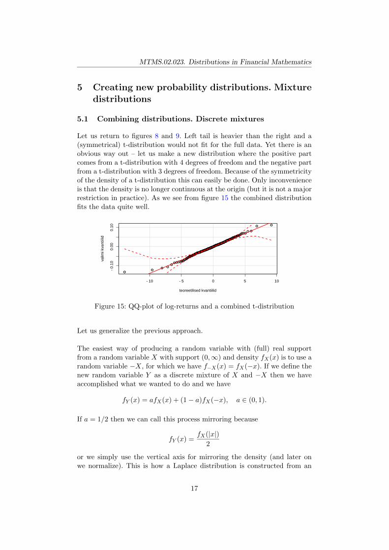
Let us return to figures 8 and 9. Left tail is heavier than the right and a(symmetrical) t-distribution would not fit for the full data. Yet there is anobvious way out – let us make a new distribution where the positive partcomes from a t-distribution with 4 degrees of freedom and the negative partfrom a t-distribution with 3 degrees of freedom. Because of the symmetricityof the density of a t-distribution this can easily be done. Only inconvenienceis that the density is no longer continuous at the origin (but it is not a majorrestriction in practice). As we see from figure 15 the combined distributionfits the data quite well.
−10 −5 0 5 10
−0.
100.
000.
10
teoreetilised kvantiilid
valim
i kva
ntiil
id
●●
● ●●
●●●●●●●●●●
●●●●●●●●●●●●
●●●●●●●●●●●●●●●●●●●●●
●●●●●●●●●●●●●●●●●●●●●●●●●●●●●●●●●●●●●●●●●●●●●●●●●●●●●●●●●●●●●●●●●●●●●●●●●
●●●●●●●●●●●●●●●●●●●●●●●●●●●●●●●●●●●●●●●●●●●●●●●●●●●●●●●●●●●●●●●●●●●●●●●●●●●●●●●●●●●●●●●●●●●●●●●●●●●●●●●●●●●●●●●●●●●●●●●●●●●●●●●●●●●●●●●●●●●●●●●●●●●●●●●●●●●●●●●●●●●●●●●●●●●●●●●●●●●●●●●●●●●●●●●●●●●
●●●●●●●●●●●●●●●●●●●●●●●●●●●●●●●●●●●●●●●●●●●●●●●●●●●●●●●●●●●●●●●●●●●●●●●●●●●●●●●●●●●●●●●●●●●●●●●●●●●●●●●●●●●●●●●●●●●●●●●●●●●●●●●●●●●●●●●●●●●●●●●●●●●●●●●●●●●●●●●●●●●●●●●●●●●●●●●●●●●●●●●●●●●●●●●●●●●●●●●●●●●●●●●●●●●●●●●●●●●●●●●●●●●●●●●●●●●●●●●●●●●●●●●●●●●●●●●●●●●●●●●●●●●●●●●●●●●●●●●●●●●●●●●●●●●●●●●●●●●●●●●●●●●●●●●●●●●●●●●●●●●●●●●●●●●●●●●●●●●●●●●●●●●●●●●●●●●●●●●●●●●●●●●
●●●●●●●●●●●●●●●●●●●●●●●●●●●●●●●●●●●●●●●●●●●●●●●●●●●●●●●●●●●●●●●●●●●●●●●●●●●●●●●●●●●●●●●●●●●●●●●●●●●●●●●●●●●●●●●●●●●●●●●●●●●●●●●●●●●●●●●●●●●●●●●●●●●●●●●●●●●●●●●●●●●●●●●●●●●●●●●●●●●●●●●●●●●●●●●●●●●●●●●●●●●●●●●●●●●●●●●●●●●●●●●●●●●●●●●●●●●●●●●●●●●●●●●●●●●●●●●●●●●●●●●●●●●●●●●●●●●●●●●●●●●●●●●●●●●●●●●●●●●●●●●●●●●●●●●●●●●●●●●●●●●●●●●●●●●●●●●●●●●●●●●●●●
●●●●●●●●●●●●●●●●●●●●●●●●●●●●●●●●●●●●●●●●●●●●●●●●●●●●●●●●●●●●●●●●●●●●●●●●●●●●●●●●●●●●●●●●●●●●●●●●●●●●●●●●●●●●●●●●●●●●●●●●●●●●●●●●●●●●●●●●●●●●●●●●●●●
●●●●●●●●●●●●●●●●●●●●●●●●●●●●●●●●●●●●●●●●●●●●●●●●●●
●●●●●●●●●●●●●●●●●●●
●●●●●●●●
●●●● ●
● ●
Figure 15: QQ-plot of log-returns and a combined t-distribution
Let us generalize the previous approach.
The easiest way of producing a random variable with (full) real supportfrom a random variable X with support (0,∞) and density fX(x) is to use arandom variable −X, for which we have f−X(x) = fX(−x). If we define thenew random variable Y as a discrete mixture of X and −X then we haveaccomplished what we wanted to do and we have
fY (x) = afX(x) + (1− a)fX(−x), a ∈ (0, 1).
If a = 1/2 then we can call this process mirroring because
fY (x) =fX(|x|)
2
or we simply use the vertical axis for mirroring the density (and later onwe normalize). This is how a Laplace distribution is constructed from an
17
MTMS.02.023. Distributions in Financial Mathematics
exponential distribution. It is obvious than when X has a heavy right tailthen both right and left tail of Y are heavy (similarly light tail of X). Thusthe Laplace distribution has light tails. Of course we can also paste togetherpieces that are not symmetrical (just like we did with the t-distribution).
Just as easy as this pasting operation is the division of a random variablethat has support on the whole R. If the density fZ(x) of a random variableZ is symmetrical then we can easily define a random variable W for whichfW (x) = 2fZ(x)I(0,∞).
Discrete mixture can be made from arbitrary distributions (we can even useboth discrete distributions and continuous distributions). We can do thisby making use of indicator functions that do not overlap. This is known assplicing. But we can use densities that have overlapping support and create,e.g., multimodal distributions.
Let f1(x),. . . ,fi(x),. . . ,fk(x) be density functions with non-overlapping sup-ports (c0, c1),. . . ,(ck−1, ck), respectively. If we take positive constants a1, . . . , ak,such that a1 + . . .+ ak = 1, then a k-component spliced density is
fX(x) =
a1f1(x), c0 < x < c1,
a2f2(x), c1 < x < c2,
. . .
akfk(x), ck−1 < x < ck,
with support (c0, ck).
Typically the distributions used for splicing do not have such nice densities.Then we must normalize the probability density functions using the cu-mulative distribution functions. Thus we must replace fj(x) with the ratiofj(x)/[Fj(cj)− Fj(cj−1)] for all j = 1, . . . , k.
Most general way of defining a discrete mixture is the following.
Definition 5.1. Let X1, X2, . . . be random variables with respective cu-mulative distribution functions FX1(x), FX2(x), . . .. We say that a randomvariable Y is a discrete mixture of X1, X2, . . . if it holds that
FY (x) = a1FX1(x) + a2FX2(x) + . . . ,
where ai > 0 and∑ai = 1.
By the given definition, the derivation of random variable Y from randomvariables X1, X2, . . . is very straightforward. Thus the moments of Y are alsoeasy to calculate.
18
MTMS.02.023. Distributions in Financial Mathematics
5.2 Continuous mixtures
When defining a discrete mixture we do not require that the cumulativedistribution functions FX1(x), FX2(x), . . . would be similar in any way. Butwe could consider a scenario where they would all be members of the sameclass. E.g. FXi could be a cumulative distribution function of a normal dis-tribution with parameters µi ja σ2 > 0 and the weights could be definedas ai = λi
i! e−λ, where λ > 0. Such construction is the basis for continuous
mixtures where summation is replaced with integration and the weights arereplaced with a density function.
Definition 5.2. Let us have a family of random variables Xλ such thattheir distribution depends on some parameter λ, which itself is a realizationof some random variable Λ. In other words, for any fixed λ, the (conditional)density of Xλ is given by fXλ(x). Let us assume that the density fΛ(λ) ofrandom variable Λ is also known. Now, we can combine the random variablesXλ and Λ to obtain a new random variable X with the following density:
fX(x) =
∫fXλ(x)fΛ(λ)dλ.
Random variable X is called a continuous mixture of distributions of Xλ
and Λ (distribution of Λ is known as the mixing distribution).
Notice also that for any fixed λ we have Xλ = (X|Λ = λ).
Also in this case the simulation principle is simple (as long as we know howto simulate both Xλ and Λ). The cdf can be derived as follows
FX(x) =
∫ x
−∞
∫fXλ(y)fΛ(λ)dλdy
=
∫ ∫ x
−∞fXλ(y)fΛ(λ)dydλ
=
∫FXλ(x)fΛ(λ)dλ.
If the moments are of interest we can write:
E(Xk) =
∫xk∫fXλ(x)fΛ(λ)dλdx
=
∫ (∫xkfXλ(x)dx
)fΛ(λ)dλ
=
∫E(Xk
λ)fΛ(λ)dλ
= E[E(Xk|Λ)].
19

MTMS.02.023. Distributions in Financial Mathematics
Home assignment 10. Consider an exponential distribution with param-eter λ > 0 and probability density function
f1(x) = λe−λx, x > 0.
Now let λ have a Γ-distribution with parameters α > 1 and θ > 0, i.e. itsdensity function is
f2(x) =θα
Γ(α)xα−1e−θx, x > 0.
Find the cumulative distribution function, probability density function andmean of this continuous mixture distribution.
5.3 Completely new parts
Theoretically, there is no need to use any particular known distributionwhen constructing our approximation (perhaps it would be more preciseto say ”any particular known distribution that we are aware of” becauseprobably somebody somewhere has already used such a distribution). Weknow that distributions with a continuous cumulative distribution functioncan be simulated by making use of an uniform distribution and applying theinverse of the cumulative distribution function to (the realization of) thisdistribution. This also means that we can make continuous distributionsapplying invertible functions to the uniform distribution. The cumulativedistribution function of any such distribution is easy to write down and thusthe probability density function is straightforward also.
E.g. we can consider the transformation
Y =(− lnU)−ξ − 1
ξ,
where U is a random variable with standard uniform distribution and ξ ∈ R.When ξ = 0 then we interpret this as
− ln(− lnU),
noting that (1 + x/n)n → exp(x) and for positive arguments n(x1/n − 1)→lnx. The support of random variable Y is thus (−∞,−1/ξ), if ξ < 0 and(−1/ξ,∞) if ξ > 0. If ξ = 0, the support is the whole real line.
If we want to calculate the moments of Y then we should notice that − lnUis a random variable with standard exponential distribution. Using the New-
20
MTMS.02.023. Distributions in Financial Mathematics
ton’s binomial formula we obtain that
EY n = E(
(− lnU)−ξ − 1
ξ
)n= E
n∑k=0
Ckn
[(− lnU)−ξ
ξ
]k (−1
ξ
)n−k=
n∑k=0
Ckn
(−1
ξ
)nE[(− lnU)−ξk
],
i.e. we need to find the (not necessarily integer) moments of an exponentialdistribution and this allows us to calculate the moments of the new randomvariable.
5.4 Parameters of a distribution
In the previous we considered some possibilities of producing ”new” distri-butions to get an approximation that would fit our data well. This idea isnice because using the tools from the preceding an array of very diverse dis-tributions can be generated. There is a danger, however: if the model fits the(training) data well then we might discover that it does not fit the new (test)data. The reason for this is the stochasticity of a sample – every sample hasits own particularities. If we include this into the model then the model willnot fit any other sample. This is known as over-fitting. So how do we avoidthis? By not using too complex models. But also by using common sense.What this means in particular will be discussed in what follows.
But a quick simple example can be given if we think about the previousexamples and consider the amount of model parameters involved. For acombined t-distribution we have only two parameters – one for the rightand the other for the left tail. But we could also consider that the weightswould not be equal (e.g. more gains than losses). Then an additional weightparameter a is required:
fY (x) = afX1(x) + (1− a)fX2(x), a ∈ (0, 1).
and there are 3 parameters in total. Now perhaps we would like to allowthat the ”pasting point” (the point where the two pieces are joined) is notnecessarily the origin so another parameter would then have to be added.This would mean 4 parameters and all of them should then (typically) beestimated from the data.
Home assignment 11. How many parameters are present in a (general)discrete mixture of five normal distributions? What is the minimal amountof parameters that can be retained in particular context?
21

MTMS.02.023. Distributions in Financial Mathematics
6 Empirical distribution. Kernel density estima-tion
Let us recall that in our log-returns example we concluded that a normaldistribution is not a suitable model. To illustrate this, densities were com-pared: we estimated the parameters of a normal distribution based on thedata but we also used the data to estimate the density directly (using kerneldensity estimation). We will now pay more attention to the latter as it seemslike a very appealing method – assumptions are minimal and we only ”letthe data speak”. To explain the ideas of kernel density estimation we willfirst recall the concept of empirical distribution.
Empirical distribution is the distribution based on a sample and its cumu-lative distribution function can be found as follows.
Definition 6.1 (Empirical cumulative distribution function). Empirical cu-mulative distribution function of a sample x1, . . . , xn is defined as
Fn(x) ={#xi : xi 6 x}
n.
The empirical cumulative distribution function is a step function like thecumulative distribution functions of discrete distributions. The reason forthis is the fact that for any finite sample size n the empirical distribution isdiscrete.
Now, if we need to visualize the underlying theoretical density based on asample, a natural starting point would be the probability mass function ofthe sample. Unfortunately, such graph would only consist of bars with equalheight 1
n (if there are no duplicates in the sample). Obviously, more probableregions have more bars, but it is still hard to understand the specifics of theunderlying distribution from such graph. Therefore, certain aggregation ofsome sample elements might be a reasonable choice.
We consider the following setup. First we find the sample minimum andmaximum. Then we divide the interval between them into subintervals withequal length (the left-most is a closed interval and the others do not includethe left endpoint). We count for each interval how many values fall into theinterval and represent these frequencies by bars (more frequent classes arerepresented by higher bars). If the sample size and the number of intervals areboth large then this graph (histogram) reminds us a density function whichis divided into classes. This is how Figure 6 has been obtained based on thepositive log-returns sample. Actually such a graph does not approximate adensity function because the area under the graph is not equal to one. But ifwe were to increase the number of intervals then both would have the sameshape (but not scale).
22
MTMS.02.023. Distributions in Financial Mathematics
So, if we would like the histogram to represent or estimate the density, weneed to transform the scale. But this is actually not the goal of a histogram,it is usually sufficient to get the idea about the shape.
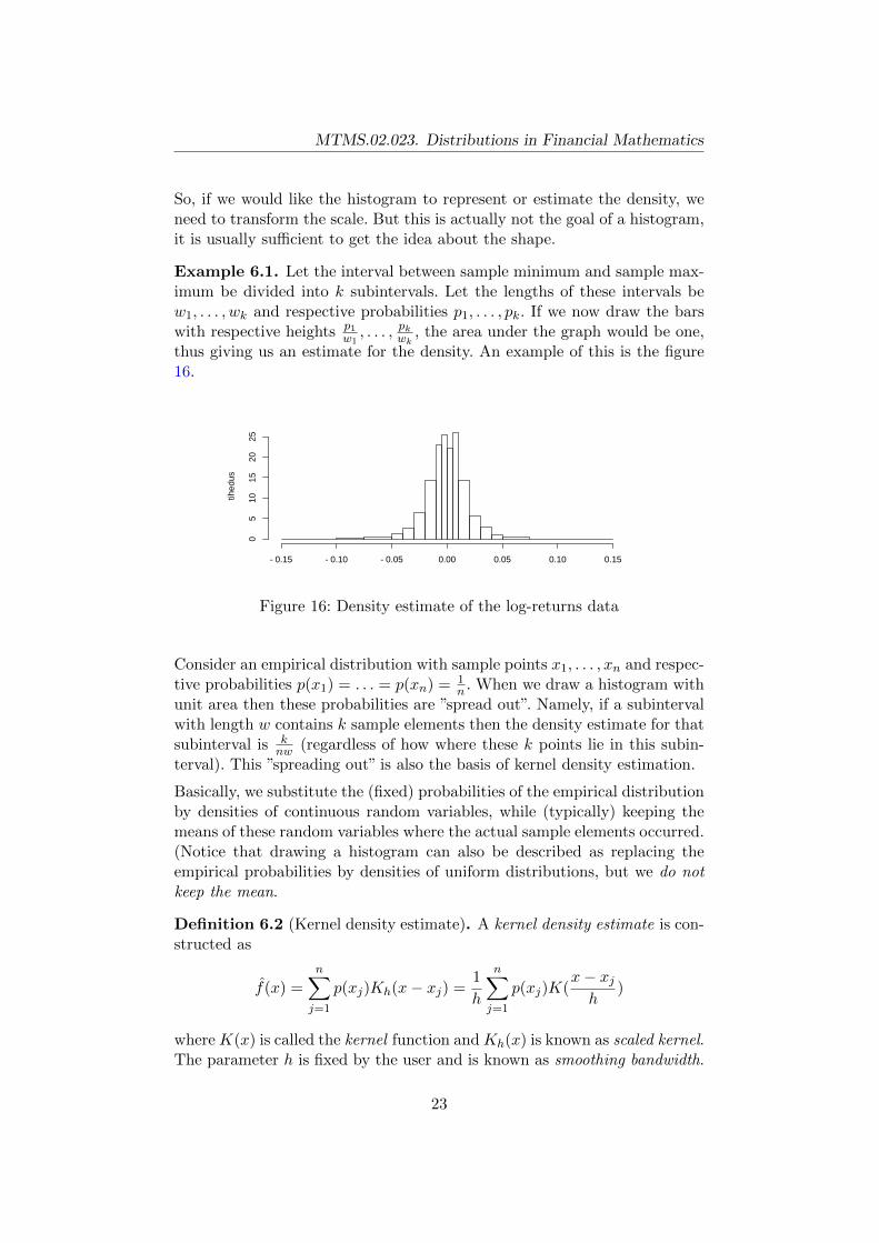
Example 6.1. Let the interval between sample minimum and sample max-imum be divided into k subintervals. Let the lengths of these intervals bew1, . . . , wk and respective probabilities p1, . . . , pk. If we now draw the barswith respective heights p1
w1, . . . , pkwk , the area under the graph would be one,
thus giving us an estimate for the density. An example of this is the figure16.
tihed
us
−0.15 −0.10 −0.05 0.00 0.05 0.10 0.15
05
1015
2025
Figure 16: Density estimate of the log-returns data
Consider an empirical distribution with sample points x1, . . . , xn and respec-tive probabilities p(x1) = . . . = p(xn) = 1
n . When we draw a histogram withunit area then these probabilities are ”spread out”. Namely, if a subintervalwith length w contains k sample elements then the density estimate for thatsubinterval is k
nw (regardless of how where these k points lie in this subin-terval). This ”spreading out” is also the basis of kernel density estimation.
Basically, we substitute the (fixed) probabilities of the empirical distributionby densities of continuous random variables, while (typically) keeping themeans of these random variables where the actual sample elements occurred.(Notice that drawing a histogram can also be described as replacing theempirical probabilities by densities of uniform distributions, but we do notkeep the mean.
Definition 6.2 (Kernel density estimate). A kernel density estimate is con-structed as
f(x) =
n∑j=1
p(xj)Kh(x− xj) =1
h
n∑j=1
p(xj)K(x− xjh
)
where K(x) is called the kernel function and Kh(x) is known as scaled kernel.The parameter h is fixed by the user and is known as smoothing bandwidth.
23

MTMS.02.023. Distributions in Financial Mathematics
Thus, a scaled kernel is obtained from the ”original” kernel using the follow-ing scaling:
Kh(u) =1
hK(
u
h).
The kernel K(u) itself is typically (but not always) a symmetrical densityfunction with zero mean.
Definition 6.3 (Uniform (rectangular) kernel). Uniform kernel or rectan-gular kernel is defined as
K(u) =1
2I|u|61,
and as such the uniform kernel distributes the probability equally aroundthe original location.
Because a smoothing bandwidth 1 would be too large for our data, we willbe using percent scale in the next figures (i.e., we plot the graph of logre-turns*100 ).
Home assignment 12. Find analytically how many times the standarddeviation of K(x) increases when the smoothing bandwidth increases h > 0times.
Home assignment 13. Study the command ?density in R to learn how toset the smoothing bandwidth in R. How could we use the parameter adjustso that we would not need to transform the log-returns data into percentscale?
−15 −10 −5 0 5 10
0.00
0.10
0.20
bw=1
tihed
us
Figure 17: Kernel density estimate of log-returns using the uniform kernel(in percent scale)
Definition 6.4 (Triangular kernel). Triangular kernel is defined as
K(u) = (1− |u|)I|u|61,
thus it divides the probability so that there is linear decrease in both direc-tions.
24

MTMS.02.023. Distributions in Financial Mathematics
−15 −10 −5 0 5 10
0.00
0.10
0.20
bw=1
tihed
us
Figure 18: Kernel density estimate of log-returns using the triangular kernel(in percent scale)
Definition 6.5 (Epanechnikov kernel). Epanechnikov kernel is defined as
K(u) =3
4(1− u2)I|u|61,
thus it divides the probability so that there is quadratic decrease in bothdirections.
−15 −10 −5 0 5 10
0.00
0.10
0.20
bw=1
tihed
us
Figure 19: Kernel density estimate of log-returns using the Epanechnikovkernel (in percent scale)
Definition 6.6 (Gaussian kernel). Gaussian kernel is defined as
K(u) =1√2π
exp
{−1
2u2
},
thus it replaces the probability with a density of a normal distribution.
Thus we get a density estimate with bounded support if and only if the kernelitself has bounded support. But with unbounded kernel the tail weight (of the
25
MTMS.02.023. Distributions in Financial Mathematics
−15 −10 −5 0 5 10 15
0.00
0.05
0.10
0.15
0.20
bw=1
tihed
us
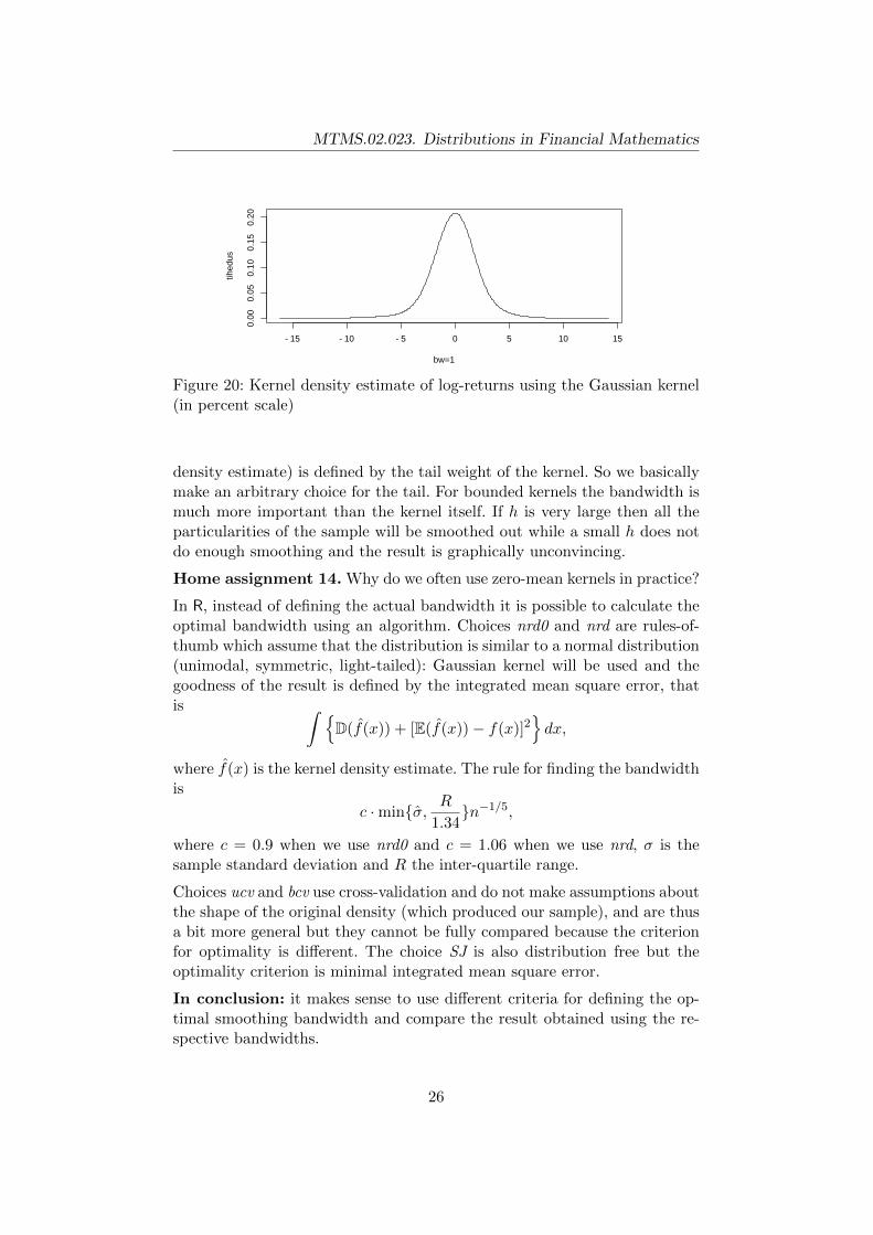
Figure 20: Kernel density estimate of log-returns using the Gaussian kernel(in percent scale)
density estimate) is defined by the tail weight of the kernel. So we basicallymake an arbitrary choice for the tail. For bounded kernels the bandwidth ismuch more important than the kernel itself. If h is very large then all theparticularities of the sample will be smoothed out while a small h does notdo enough smoothing and the result is graphically unconvincing.
Home assignment 14. Why do we often use zero-mean kernels in practice?
In R, instead of defining the actual bandwidth it is possible to calculate theoptimal bandwidth using an algorithm. Choices nrd0 and nrd are rules-of-thumb which assume that the distribution is similar to a normal distribution(unimodal, symmetric, light-tailed): Gaussian kernel will be used and thegoodness of the result is defined by the integrated mean square error, thatis ∫ {
D(f(x)) + [E(f(x))− f(x)]2}dx,
where f(x) is the kernel density estimate. The rule for finding the bandwidthis
c ·min{σ, R
1.34}n−1/5,
where c = 0.9 when we use nrd0 and c = 1.06 when we use nrd, σ is thesample standard deviation and R the inter-quartile range.
Choices ucv and bcv use cross-validation and do not make assumptions aboutthe shape of the original density (which produced our sample), and are thusa bit more general but they cannot be fully compared because the criterionfor optimality is different. The choice SJ is also distribution free but theoptimality criterion is minimal integrated mean square error.
In conclusion: it makes sense to use different criteria for defining the op-timal smoothing bandwidth and compare the result obtained using the re-spective bandwidths.
26
MTMS.02.023. Distributions in Financial Mathematics
7 Subexponential distributions
7.1 Preliminaries. Definition
Let us now consider distributions with support (0,∞). Positive random vari-ables are very popular in applications (size of an insurance claim, numberof claims etc) and it is often possible to represent the underlying randomvariable as a difference between two positive random variables (profit canbe expressed as a difference between turnover and expenses).
In particular, we concentrate on a sub-class of heavy-tailed distributions:subexponential distributions. Each distribution in this class has many niceproperties, yet the class is rich enough to include a large variety of models.In the following we study the properties of this class in more detail.
Let us first recall the concept of convolution of distributions.
Remark 7.1 (Convolution of distributions). Let Xi, i = 1, . . . , k be in-dependent random variables with distributions Pi, then the distribution ofX1+. . .+Xn (say, P ) is called the convolution of distributions Pi. Similar no-tion is used for distribution functions and probability density functions: thedistribution function FX1+...+Xn is called the convolution of (independent)distribution functions FXi and denoted by
FX1+...+Xn = FX1 ∗ FX2 ∗ . . . ∗ FXn .
If Xi-s have same distribution, the corresponding convolution is denoted byF ∗n.
For two independent random variables X and Y :
• in general: FX+Y (s) =∫FX(s− y)dFY (y);
• if X is continuous: fX+Y (s) =∫fX(s− y)dFY (y);
• if both X and Y are continuous: fX+Y (s) =∫fX(s− y)fY (y)dy.
Definition 7.1 (Subexponential distributions). Class
S = {X > 0 : ∀n ∈ N limx→∞
F ∗nX (x)
FX(x)= n}
is called the class of subexponential distributions. Here F ∗n(x) denotes then-fold convolution of a function F (x).
The name of the class is due to the fact that if X ∈ S then ∀ε > 0
limx→∞
eεxFX(x) =∞,
which means that the tail function goes to zero at a slower rate than anyexponential function of the form e−εx, where ε > 0.
27
MTMS.02.023. Distributions in Financial Mathematics
Definition 7.2 (Asymptotic equivalence (tail equivalence)). Let F (x) andG(x) be any two functions. We write F (x) ∼ G(x) and say that F (x) andG(x) are asymptotically equivalent if
limx→∞
F (x)
G(x)= 1.
7.2 Properties of subexponential class
To give some intuition about the class S let us consider a sequenceX1, . . . , Xn ∈S of iid random variables with cumulative distribution function F (x). Letus also define Sn = X1 + . . . + Xn and Mn = max(X1, . . . , Xn). Now,since P(Mn > x) = 1 − [F (x)]n and because of the asymptotic equivalence1− [F (x)]n ∼ nF (x), we obtain
P(Mn > x) ∼ P(Sn > x).
Thus for subexponential distributions ”a large sum is due to one large sum-mand”, which is very relevant in practice. Imagine the arrival of insuranceclaims. When the aggregate claim is very large then typically this is becauseof a single very large claim. This in turn means that there is no time to reactbecause we do not know in advance when the large claim might occur.
Let X1 ∈ S with cumulative distribution function FX1(x) and X2 > 0 withcumulative distribution function FX2(x) be a random variable with a lightertail i.e.
limx→∞
FX1(x)
FX2(x)=∞.
Also let X1 and X2 be independent. Then
X1 +X2 ∈ S
andFX1+X2(x) ∼ FX1(x)
So a subexponential tail is still dominant in the sum.
Let X1 ∈ S with cumulative distribution function FX1(x) and X2 > 0 withcumulative distribution function FX2(x), such that for some c > 0
cFX1(x) ∼ FX2(x).
Then also X2 ∈ S and if X1 and X2 are independent then
X1 +X2 ∈ S
andFX1+X2(x) ∼ (1 + c)FX1(x)
28
MTMS.02.023. Distributions in Financial Mathematics
So the class is closed with respect to addition.
Let X1, . . . , Xn ∈ S be iid random variables with cumulative distributionfunction F (x). From previous we know that
P(Mn > x) ∼ P(Sn > x) ∼ nF (x),
but due to the previous property we have that Sn ∈ S and Mn ∈ S, so theclass is also closed with respect to maximum.
Note that if the limit property in the definition of subexponentiality holdsfor some n ≥ 2, i.e.
limx→∞
F ∗n(x)
F (x)= n,
then the result holds for every n ≥ 2. Thus, to check whether a randomvariable X belongs to the class of subexponential distributions, X ∈ S, it issufficient to find only one limit. But even this can be complicated in reality.
Often a Pitman condition is used instead to check if a distribution is in S:Let X > 0 be a random variable with probability density function f(x) andhazard function h(x), which is eventually decreasing and for which we havelimx→∞
h(x) = 0. If ∫ ∞0
exh(x)f(x)dx <∞,
then X ∈ S.
Home assignment 15. Let X1 and X2 be random variables with respectiveprobability density functions f1(x) and f2(x). Show that X1, X2 ∈ S.
1. f1(x) = αθα
(x+θ)α+1 , α > 0, θ > 0, x > 0
2. f2(x) = kλ
(xλ
)k−1e−( xλ)
k
, λ > 0, 0 < k < 1, x > 0
It is allowed to take θ = 1 and λ = 1. Using the knowledge about the tails,why does it make sense that a random variable X3 with probability densityfunction
f3(x) =1
xσ√
2πe−
(ln x−µ)2
2σ2 , µ ∈ R, σ > 0, x > 0,
is a subexponential distribution?
29
MTMS.02.023. Distributions in Financial Mathematics
8 Well-known distributions in financial and insur-ance mathematics
In this section we recall some common distributions used in financial andinsurance mathematics.
8.1 Exponential distribution
Exponential distribution is a widely used distribution in the theory of stochas-tic processes – it is the probability distribution that describes the time be-tween events in a Poisson process (process in which events occur continuouslyand independently at a constant average rate).
For an exponentially distributed random variable X we write X ∼ E(λ) (orX ∼ Exp(λ)), where λ > 0 is a rate (or inverse scale) parameter.
The key property of exponential distribution is being memoryless. Only ex-ponential and geometric distributions have the property of being memory-less:
P{X ≥ t+ s|X ≥ s} = P{X ≥ t}.
Main characteristics for the exponential distribution are:
• probability density function fX(x) = λe−λx, x ≥ 0,
• cumulative distribution function FX(x) = 1− e−λx, x ≥ 0,
• expectation EX = 1λ ,
• variance V arX = 1λ2
,
• mode argmax f(x) = 0,
• median med X = ln 2λ ,
• the sum of independent exponential random variables with same pa-rameter λ is a gamma-distributed random variable: X1, . . . , Xn ∼E(λ)⇒
∑nk=1 ∼ Γ(n, λ),
• the minimum of independent exponential random variables is also ex-ponentially distributed: X1, . . . , Xn ∼ E(λ) ⇒ min{X1, . . . , Xn} ∼E(λ1 + . . .+ λn).
The following list contains few examples of applications where exponentialdistribution can be used.
30

MTMS.02.023. Distributions in Financial Mathematics
• The exponential distribution occurs naturally when describing thelengths of the inter-arrival times in a homogeneous Poisson process.It describes the time for a continuous process to change state.
• In situations where certain events occur with a constant probabilityper unit length, for example, number of phone calls received in fixedtime period.
• In queuing theory, the service times of agents in the system are oftenmodeled as exponentially distributed variables.
• In physics, if you observe a gas at a fixed temperature and pressure ina uniform gravitational field, the heights of the various molecules alsofollow as approximate exponential distribution, known as Barometricformula.
• In hydrology, the exponential distribution is used to analyze extremevalues of such variables as monthly and annual maximum values ofdaily rainfall and river discharge volumes.
8.2 Pareto distribution
The Pareto distribution is a power law probability distribution that is usedin several models in economics and social sciences. The corresponding distri-bution family is a wide one, with several sub-families. We will first review theclassical Pareto distribution and then focus on it’s shifted version (so-calledAmerican Pareto distribution), which is most widely used in non-life insur-ance as a model for claim severity. The distribution is named after italiansociologist and economist Vilfredo Pareto (who is also the author of the 80-20 principle). Nowadays Pareto distribution is widely used in description ofsocial, scientific, geophysical, actuarial, and many other types of observablephenomena
A. The classical Pareto, Z ∼ Pa∗(α, β), α, β > 0
Main characteristics for the classical Pareto distribution are:
• probability density function fZ(z) = αβα
zα+1 , z ≥ β,
• cumulative distribution function FZ(z) = 1−(βz
)α, z ≥ β,
• expectation EZ = αβα−1 , α > 1,
• variance V arZ = αβ2
(α−1)2(α−2), α > 2,
• moments EZn = αβn
α−n , α > n, but EZn =∞, α ≤ n.
31

MTMS.02.023. Distributions in Financial Mathematics
B. American Pareto, X ∼ Pa(α, β), X = Z−β, Z ∼ Pa∗(α, β), α, β > 0
The American Pareto distribution is obtained from classical Pareto distri-bution by shifting it to the origin.
Main characteristics for the American Pareto distribution are:
• probability density function fX(x) = αβα
(β+x)α+1 , x ≥ 0,
• cumulative distribution function FX(x) = 1−(
ββ+x
)α, x ≥ 0,
• expectation EX = βα−1 , α > 1,
• variance V arX = αβ2
(α−1)2(α−2), α > 2,
• moments EXn = βnn!∏ni=1(α−i) , α > n, but EXn =∞, α ≤ n,
• U ∼ U(0, 1)⇒ β(U−1/α − 1) ∼ Pa(α, β),
• mode argmax f(x) = 0,
• median med X = β(21/α − 1).
Parameter estimation using the method of moments:
α =2(m2 −m2
1)
m2 − 2m21
,
β =m1m2
m2 − 2m21
,
where m1 =∑n
j=1xjn and m2 =
∑nj=1
x2jn .
0 2 4 6 8 10
0.0
0.5
1.0
1.5
2.0
x
f(x)
Pa(1,1)Pa(2,1)Pa(1,2)
Figure 21: Pareto density under several parameter combinations
Home assignment 16. Suppose we have an iid sample X1, . . . , Xn fromPa(α, β). What is the distribution of min{X1, . . . , Xn}?
32
MTMS.02.023. Distributions in Financial Mathematics
Pareto distribution is not limited to describing wealth or income, it is widelyused in describing social, scientific, geophysical and many other types ofobservable phenomena, for example:
• the size of human settlement (many villages, few cities),
• file size of internet traffic that uses the TCP protocol,
• hard disk drive error rates,
• values of oil reserves in oil fields,
• standardized price returns on individual stocks,
• sizes of sand particles,
• sizes of meteorites,
• areas burnt in forest fires.
8.3 Weibull Distribution
The Weibull distribution is of interest in various fields, ranging from life datato weather data or observations made in economics and business administra-tion, in hydrology, in biology or in the engineering science. The distributionis named after the Swedish physicist Waloddi Weibull who used it in relia-bility testing of materials.
For a random variable X that follows Weibull distribution we write X ∼We(k, λ), where k > 0 is a shape parameter and λ > 0 is a scale parameter.
The main characteristics of the distribution are
• probability density function fX(x) = kλ
(xλ
)k−1e−( xλ)
k
, x ≥ 0,
• cumulative distribution function F (x) = 1− e−( xλ)k
,
• E(Xn) = λnΓ(1 + nk ),
• E|X|n <∞,
• U ∼ U(0, 1)⇒ λ(− lnU)1/k ∼We(k, λ),
• mode argmax f(x) = λ(k−1k
)1/kI{k>1},
• median med X = λ(ln 2)1/k.
33
MTMS.02.023. Distributions in Financial Mathematics
0 2 4 6 8 10
0.0
0.5
1.0
1.5
2.0
x
f(x)
We(1,1)We(0.5,1)We(1,2)
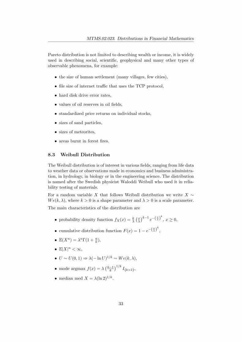
Figure 22: Weibull density under several parameter combinations
We also note that if
k < 1, then Weibull distribution is “between” exponential and Pareto;k > 1, then Weibull distribution has lighter tail than exponential;k = 1, then Weibull distribution reduces to exponential.
Remark. In order to stress the relation to exponential distribution, Weibulldistribution is often parametrized by k and θ = 1
λ , implying the following:
• cumulative distribution function FX(x) = 1− e−θxk ,
• probability density function fX(x) = kθkxα−1e−θxk.
8.4 Lognormal distribution
Lognormal distribution plays the role of normal distribution in the multi-plicative central limit theorem (we multiply iid random variables). When thelogarithm of a random variable has a normal distribution then the randomvariable itself has a lognormal distribution. Thus, the distribution functionof lognormal distribution is found using the log transformation to reachnormal distribution and standardization to reach standard normal distribu-tion. Since the normal distribution is one of the most thoroughly studieddistributions, the simple connection between lognormal and normal makeslognormal distribution also an appealing choice in different models.
For a lognormally distributed random variable X we write X ∼ LnN(µ, σ)(or X ∼ Ln(µ, σ)), where −∞ < µ <∞ is a location parameter and σ > 0is a scale parameter.
Main characteristics are:
• its connection to normal distribution, if Y ∼ N(µ, σ) and X = eY ,then X = LnN(µ, σ),
34

MTMS.02.023. Distributions in Financial Mathematics
• cumulative distribution function FX(x) = FY (lnx) = Φ( lnx−µσ ),
• probability density function fX(x) = 1xfY (lnx),
• expectation EX = eµ+σ2
2 ,
• variance V arX = e2µ+σ2(eσ
2 − 1),
• moments EXn = enµ+ 12n2σ2
,
• E|X|n <∞,
• Y ∼ N(0, 1)⇒ eµ+σY ∼ LnN(µ, σ2),
• mode argmax f(x) = eµ−σ2,
• median med X = eµ.
Parameter estimation:
µ =1
n
n∑j=1
lnxj ,
σ2 =1
n− 1
n∑j=1
[ln(xj − µ)]2.
0 2 4 6 8 10
0.0
0.2
0.4
0.6
0.8
1.0
x
f(x)
Ln(0,1)Ln(2,1)Ln(0,0.5)
Figure 23: Log-normal density under several parameter combinations
8.5 Log-gamma distribution
A random variable is log-gamma distributed if its natural logarithm is gamma-distributed. Notice that as a gamma-distributed random variable can onlytake non-negative values, the support of log-gamma distribution is [−1;∞)
For a log-gamma distributed random variable we write X ∼ Lg(α, β), whereα > 0 is the rate parameter (of corresponding gamma distribution) andβ > 0 is a shape parameter.
35

MTMS.02.023. Distributions in Financial Mathematics
2 4 6 8 10
0.0
0.5
1.0
1.5
2.0
x
f(x)
Lg(1,1)Lg(2,1)Lg(1,2)
Figure 24: Log-gamma density under several parameter combinations
The main characteristics of the log-gamma distribution are:
• probability density function fX(x) = αβ(lnx)β−1
Γ(β)xα+1 , x ≥ 1,
• cumulative distribution function F (x) does not have analytic expres-sion,
• E(Xn) =(
αα−n
)β,
• E|X|n <∞⇔ n < α,
• Y ∼ Γ(α, β)⇒ eY ∼ Lg(α, β),
• mode argmax f(x) = eβ−1α+1
I{β>1} ,
• median med X does not have analytic expression.
8.6 Burr distribution
In probability theory, statistics and econometrics, the Burr Type XII dis-tribution or simply the Burr distribution is a continuous probability distri-bution for a non-negative random variable. It is also known as the Singh-Maddala distribution and is one of a number of different distributions, some-times called the ”generalized log-logistic distribution”, as it contains the log-logistic distribution as a special case. It is most commonly used to modelhousehold income. The distribution is named after american statistician Irv-ing W. Burr.
For a Burr distributed random variable X we write X ∼ Bu(c, α), wherec > 0 and α > 0.
Main characteristiscs of the Burr distribution are:
36

MTMS.02.023. Distributions in Financial Mathematics
0 2 4 6 8 10
0.0
0.5
1.0
1.5
2.0
x
f(x)
Bu(1,1)Bu(0.8,1)Bu(2,1)
Figure 25: Burr density under several parameter combinations
• probability density function fX(x) = αcxc−1
(1+xc)α+1 , x ≥ 0,
• cumulative distribution function FX(x) = 1−(
11+xc
)α,
• moments E(Xn) = αΓ(α−n/c)Γ(1+n/c)Γ(α+1) ,
• E|X|n <∞⇔ n < cα,
• U ∼ U(0, 1)⇒ (U−1/α − 1)1/c ∼ Bu(c, α),
• mode argmax f(x) = c−1(cα+1)1/c
I{c>1},
• median med X =(21/α − 1
)1/c.
Home assignment 17. Let X ∼ Bu(c, 1), find the distribution of 1X .
37

MTMS.02.023. Distributions in Financial Mathematics
9 Introduction to the extreme value theory (EVT)
9.1 Preliminaries. Max-stable distributions
Previously we have considered some heavy-tailed distributions which shouldfit financial data. Justification is based on the quality of the fit, typicallythere are no theoretical grounds (e.g. we probably do not believe that thet-distribution based model is actually the one generating the log-returns)and this is very common in modelling practice. We introduce the tools ofEVT which actually have theoretical justification as models in certain (andnot uncommon) situations.
Definition 9.1. We say that two random variables X and Y (and thecorresponding distributions and distribution functions) are of the same typeif there exist constants a > 0 and b ∈ R such that
Yd= aX + b.
In other words, if X ∼ F1(x) and Y ∼ F2(x) then
∀x F1(x) = F2(ax+ b).
Based on this definition the random variables X and aX+ b are of the sametype, i.e. changing the scale and/or location parameter does not change thetype of the distribution.
Home assignment 18. Are two normal distributions with different param-eters of the same type? What about two Pareto distributions?
Definition 9.2. A non-degenerate random variable X (and the correspond-ing distributions and distribution functions) is called max-stable if
max(X1, . . . , Xn)d= cnX + dn
for iid X,X1, . . . , Xn, appropriate constants cn > 0, dn ∈ R and every n ≥ 2.
For corresponding distribution function F (x) this means
[F (x)]n = F (cnx+ dn).
So, a max-stable distribution is a distribution for which the maximum of aniid sample has distribution of the same type.
Theorem 9.1 (Convergence to types theorem). Let X1, X2, . . . be randomvariables and an > 0, αn > 0, bn, βn ∈ R be constants. Let us also assumethat X and Y are non-degenerate and suppose the following holds
Xn − bnan
d→ X.
38

MTMS.02.023. Distributions in Financial Mathematics
ThenXn − βnαn
d→ Y (9.1)
holds if and only if
anαn→ a ∈ (0,∞),
bn − βnαn
→ b ∈ R.
If (9.1) holds then Yd= aX + b, i.e. X and Y are of the same type.
This means that when we change the normalizing constants then we mightobtain a different limiting distribution (i.e. different parameters) but thisdistribution is of the same type as the initial limiting distribution.
Let us now consider a common problem: given iid X1, . . . , Xn we need tostudy the behaviour of Mn = max{X1, . . . , Xn}. If P(Xi 6 x) = F (x), wehave P(Mn 6 x) = [F (x)]n.
We can see that Mn → xF = sup{x | F (x) < 1} and the limiting distributionis degenerate.
A more viable option is to consider certain normalized random variable ofthe same type:
Mn − bnan
and study whether a sequence of such variables can have a non-degeneratelimit. Let us call this limiting distribution G(x) an extreme value distribu-tion.
Remark 9.1. Recall that for sum Sn =∑n
i=1Xi we also have Sn → ∞,yet due to a normalization we still can obtain a non-degenerate limit. Bysubtracting the mean and dividing by the standard deviation we make surethat the expectation and variance of Sn do not grow out of control.
Theorem 9.2 (Max-stable distributions are weak limits of maxima). Anon-degenerate distribution G(x) is max-stable distribution if and only if itis an extreme value distribution (i.e. it is a limit of distributions for Mn−bn
anwhere Mn = max(X1, . . . , Xn), Xi ∼ F are iid random variables, an > 0and bn ∈ R).
Proof. A. Extreme value distributions are max-stable.
Suppose that P(Mn−bnan
6 x)→ G(x). Let us look at N independent samplesfrom distribution F , each with n elements. So we have Nn elements from Fand can derive
P(MNn − bn
an6 x
)= [P(Mn 6 anx+ bn)]N → [G(x)]N .
39
MTMS.02.023. Distributions in Financial Mathematics
On the other hand, we can also write
P(MNn − bNn
aNn6 x
)→ G(x).
Now, applying the convergence of types theorem, it follows that [G(x)]N =G(cNx + dN ), where an/aNn → cN > 0 and (bn − bNn)/aNn → dN . So, anextreme value distribution is necessarily max-stable.
B. Max-stable distributions are extreme value distributions.
Now, let us consider a random variable Z with max-stable distribution G(x).Let X1, . . . , Xn be iid copies of Z. Then, by definition of max-stable distri-butions:
max(X1, . . . , Xn)d= cnZ + dn
for some cn > 0, dn ∈ R and every n ≥ 2. Now, this implies that
Mn − dncn
d= Z,
and obviously Z is the limit of this sequence, which means that Z has ex-treme value distribution.
9.2 Forms of max-stable distributions
Let us find the explicit forms of distribution functions of max-stable distri-butions. We depart from the equation [G(x)]N = G(cNx+ dN ), which holdsfor ∀N ∈ N.
Let us first assume that cN = 1 (for ∀N). In that case
[G(x)]NM = [G(x+ dN )]M = G(x+ dN + dM )
and, on the other hand
[G(x)]NM = G(x+ dNM ),
which together imply that dN = K1 lnN . Now taking a logarithm twice(note that lnG(x) 6 0) we get
lnN + ln(− lnG(x)) = ln(− lnG(x+K1 lnN)),
so if the argument is increased byK1 lnN then the function value is increasedby lnN . Thus
ln(− lnG(x)) = K2 +x
K1,
40
MTMS.02.023. Distributions in Financial Mathematics
where K1 must be negative, because ln(− lnG(x)) is a decreasing function.
Now the distribution function is given by G(x) = exp(− exp( x
K1+K2)
),
which is of the same type as
G(x) = e−e−x.
Thus we have found the first type of max-stable distributions.
Now, let us start again with the equation [G(x)]N = G(cNx + dN ), whichholds for ∀N ∈ N. If cN 6= 1 then for x = dN (1 − cN )−1 it holds thatx = cNx+ dN , i.e. [G(x)]N = G(x) holds. This implies that
G(dN (1− cN )−1) =
{0
1.
Let us first consider G(dN (1 − cN )−1) = 1. Then the chosen point x mustbe the right endpoint of the distribution, let us denote it by xF . We cantake xF = 0, because such a distribution G(x) certainly exists in the fam-ily of distributions and we are only interested in the general form of thedistribution. So dN = xF (1− cN ) = 0. Now simple derivations
[G(x)]NM = [G(cNx)]M = G(cMcNx)
and[G(x)]NM = G(cNMx)
lead us to cN = NK1 . Taking the logarithm twice from the departing equa-tion (note again that lnG(x) 6 0) we get
lnN + ln(− lnG(x)) = ln(− lnG(NK1x))
or when the argument is increased by NK1 times then the value of thefunction is increased by lnN . Thus
ln(− lnG(x)) = ln K1√xK2,
where K2 < 0 (because the term under the root must be positive) andK1 > 0, because ln(− lnG(x)) is a decreasing function. We now get thatG(x) = exp(− K1
√xK2) which is of the same type as
G(x) = e−(−x)α , α > 0, x < 0,
and we have found our second max-stable distribution.
Let us now consider the case when G(dN (1− cN )−1) = 0. This means thatthe corresponding point is the left endpoint of the distribution, let us denote
41

MTMS.02.023. Distributions in Financial Mathematics
it by xS . As previously, without the loss of generality we can take xS = 0.This implies dN = xS(1− cN ) = 0 and further
[G(x)]NM = [G(cNx)]M = G(cMcNx)
and[G(x)]NM = G(cNMx),
resulting in cN = NK1 . Now, similarly to previous, we get
lnN + ln(− lnG(x)) = ln(− lnG(NK1x)),
from whichln(− lnG(x)) = ln K1
√xK2,
where K2 > 0 and K1 < 0, because ln(− lnG(x)) is a decreasing function.Now the formula for G(x) is G(x) = exp(− K1
√xK2), which is of the same
type asG(x) = e−(x−α), α > 0, x > 0.
This is the third and final max-stable distribution.
In summary, we have covered all possible scenarios and thus there can be nomore max-stable distributions (and thus also extreme value distributions).
9.3 Extreme value theorem. Examples
Based on the results obtained in previous subsection, we can formulate thefollowing theorem, which is known as the basis of classical extreme valuetheory.
Theorem 9.3 (Extreme value theorem/ Extremal types theorem/ Fish-er-Tippett theorem/ Fisher-Tippett-Gnedenko theorem). Let X1, X2, . . . bea sequence of iid random variables and let Mn = max(X1, . . . , Xn). If thereexist norming constants cn > 0, dn ∈ R and some non-degenerate distribu-tion function G(x) such that
P(Mn − dn
cn6 x
)→ G(x) (9.2)
then the limit distribution G(x) belongs to the type of one of the followingthree distribution functions:
• Frechet:
Φα(x) =
{0, x ≤ 0, α > 0
exp(−x−α), x > 0, α > 0
42

MTMS.02.023. Distributions in Financial Mathematics
• Weibull
Ψα(x) =
{exp(−(−x)α), x ≤ 0, α > 0
1, x > 0, α > 0
• GumbelΛ(x) = exp(−e−x)
Generalized extreme value (GEV) distribution is a distribution that includesall three obtained classes and provides a unified parametrization for them.
Definition 9.3 ((Maximum) domain of attraction). We say that a randomvariable X (and the corresponding distribution and distribution function)belong to the maximum domain of attraction of the extreme value distri-bution G(x) if there exist constants cn > 0 and dn ∈ R such that (9.2)holds.
Based on this definition and extreme value theorem, we can formulate thefollowing result.
Corollary 9.1. There exists a four-way division of distributions into classesthat do not intersect:
1. distributions in the domain of attraction of the Frechet extreme valuedistribution;
2. distributions in the domain of attraction of the Weibull extreme valuedistribution;
3. distributions in the domain of attraction of the Gumbel extreme valuedistribution;
4. distributions which do not have a non-degenerate limiting distributionfor their sample maximum, regardless of the normalization.
Example 9.1. Let X,X1, . . . , Xn be iid uniformly distributed random vari-ables, X ∼ U(a, b). Let us take an = b−a
n and bn = b − b−an . Then, for
1− n < x < 1 we can write
P(Mn 6 anx+ bn) = (P(X ≤ anx+ bn))n =
(anx+ bn − a
b− a
)n
=
(b−an x+ b− b−a
n − ab− a
)n=
(1− 1− x
n
)n→ exp (− (1− x)) ,
which is a max-stable distribution known as the Weibull extreme value dis-tribution.
43

MTMS.02.023. Distributions in Financial Mathematics
Example 9.2. Let X,X1, . . . , Xn be iid Pareto distributed random vari-ables X ∼ Pa(α, θ), i.e. F (x) = 1 − ( θ
x+θ )α, x > 0. Let us take an = θn1/α
and bn = −θ. Then, for x > 1/nα it holds that
P(Mn 6 anx+ bn) =
[1−
(θ
θn1/αx− θ + θ
)α]n=
(1 +−(x−α)
n
)n→ exp
(−(x−α
))We recognize a max-stable distribution called Frechet’ extreme value distri-bution.
Home assignment 19. Let X1, . . . , Xn be iid exponentially distributedrandom variables, i.e. F (x) = (1 − e−λx), x > 0. As previously, let Mn
denote the running maximum Mn = max{X1, . . . , Xn}. Find the sequencesof normalizing constants an > 0 and bn, which give us the (distributional)convergence of
Mn − bnan
to a Gumbel extreme value distribution with distribution function
G(x) = e−e−x.
Also show analytically that with these normalizing constants indeed
limn→∞
P(Mn − bn
an6 x
)= G(x)
for any given value of x.
Remark 9.2. So far we only considered the right tail of a distribution, butactually the same models also apply for the left tail. This is due to simplederivation
P(min{X1, . . . , Xn} 6 x) = P(−max{−X1, . . . ,−Xn} 6 x)
= P(max{−X1, . . . ,−Xn} > −x)
Thus, if we are indeed interested in the sample minimum then we just changethe sign of our data and proceed as usual.
44
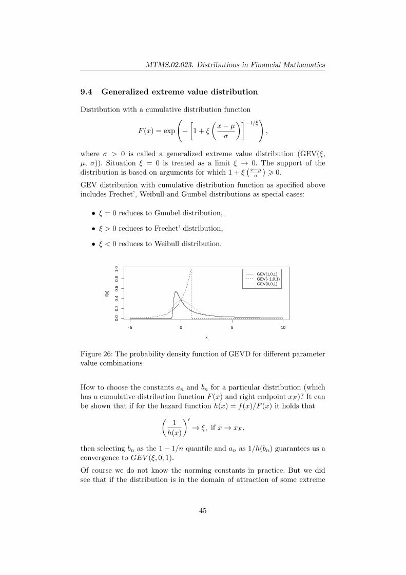
MTMS.02.023. Distributions in Financial Mathematics
9.4 Generalized extreme value distribution
Distribution with a cumulative distribution function
F (x) = exp
(−[1 + ξ
(x− µσ
)]−1/ξ),
where σ > 0 is called a generalized extreme value distribution (GEV(ξ,µ, σ)). Situation ξ = 0 is treated as a limit ξ → 0. The support of thedistribution is based on arguments for which 1 + ξ
(x−µσ
)> 0.
GEV distribution with cumulative distribution function as specified aboveincludes Frechet’, Weibull and Gumbel distributions as special cases:
• ξ = 0 reduces to Gumbel distribution,
• ξ > 0 reduces to Frechet’ distribution,
• ξ < 0 reduces to Weibull distribution.
−5 0 5 10
0.0
0.2
0.4
0.6
0.8
1.0
x
f(x)
GEV(1,0,1)GEV(−1,0,1)GEV(0,0,1)
Figure 26: The probability density function of GEVD for different parametervalue combinations
How to choose the constants an and bn for a particular distribution (whichhas a cumulative distribution function F (x) and right endpoint xF )? It canbe shown that if for the hazard function h(x) = f(x)/F (x) it holds that(
1
h(x)
)′→ ξ, if x→ xF ,
then selecting bn as the 1− 1/n quantile and an as 1/h(bn) guarantees us aconvergence to GEV (ξ, 0, 1).
Of course we do not know the norming constants in practice. But we didsee that if the distribution is in the domain of attraction of some extreme
45
MTMS.02.023. Distributions in Financial Mathematics
value distribution then for some normalization we have that a−1n (Mn−bn)
d→GEV (ξ, 0, 1). For large n thus
P(Mn − bn
an6 x
)≈ G(x).
which translates to
P(Mn 6 y) ≈ G(y − bnan
),
that is the cumulative distribution function of GEV (ξ, bn, an) which meansthat the constants are not important to us as the scale and location param-eter must be estimated anyhow.
So we saw that GEV distribution has theoretical justification as a model foriid sample maximum.
In practice, to apply GEV distribution model, the following steps can betaken:
1. We split the sample into blocks (block length is equal to the timehorizon that we are interested in).
2. We find the maximal elements of each block and form a new samplefrom these.
3. We use this new sample to estimate the parameters of a GEV distri-bution.
If we can estimate the probability that {Mn > u}, then making use of inde-pendence allows us to estimate the complementary cumulative distributionfunction as well. GEV distribution has 3 parameters and estimation thusrequires a large sample. Actually this is so also because the initial samplesize is essentially divided by the block size. But the block size cannot betaken too small because then the asymptotics behind the theory of GEVdistribution would not work.
Main properties of the GEV distribution are
• probability density function
fX(x) =1
σ
[1 + ξ
(x− µσ
)]−(ξ+1)/ξ
exp
{−[1 + ξ
(x− µσ
)]−1/ξ},
where ξ ∈ R, µ ∈ R, σ > 0,
• cumulative distribution function FX(x) = exp(−[1 + ξ
(x−µσ
)]−1/ξ),
46
MTMS.02.023. Distributions in Financial Mathematics
• moments E(Xn) =∑n
k=0Ckn
(σξ
)k (µ− σ
ξ
)n−kΓ(1− kξ),
• E|X|n <∞⇔ ξ < 1n ,
• U ∼ U(0, 1)⇒ µ+ σξ [(− lnU)−ξ − 1] ∼ GEV (ξ, µ, σ),
• mode argmax f(x) = µ+ σξ
[(1 + ξ)−ξ+ − 1
],
• median med X = µ+ σ (ln 2)−ξ−1ξ .
47
MTMS.02.023. Distributions in Financial Mathematics
9.5 Generalized Pareto distribution (GPD)
In several situations, it is more important to study the tail behaviour of adistribution.
In that case, the approximation of main part is not that important and wecan derive more efficient methods to describe the tail.
Suppose that for some µ′, σ′ and ξ we have
[F (anx+ bn)]n → exp
{−[1 + ξ · x− µ
′
σ′
]−1/ξ},
for all x. We can conclude that for some µ, σ and ξ it holds that
n ln [F (x)] ≈ −[1 + ξ · x− µ
σ
]−1/ξ
for all x. Now if x is close to the right endpoint of the distribution thenF (x) ≈ 1 and thus lnF (x) ≈ F (x)− 1. So, for large u we have
F (u) ≈ 1
n
[1 + ξ · u− µ
σ
]−1/ξ
.
Thus, for large u and y > 0 we can write that
P(X > u+ y|X > u) ≈[
1 + ξ(u+ y − µ)/σ
1 + ξ(u− µ)/σ
]−1/ξ
=
[1 +
ξy
σ + ξ(u− µ)
]−1/ξ
=
[1 +
ξy
σu
]−1/ξ
.
So, after setting the threshold, only two parameters remain. The result-ing distribution is known as the Generalized Pareto distribution (GPD).
Remark 9.3. Similarly to extreme value distributions, the GPD modelscan also applied to left tail. We can change the sign of our data (and alsothe threshold):
P(X < u− x|X < u) = P(−X > −u+ x| −X > −u),
and obtain the familiar GPD model.
How large is large u or how do we choose the threshold? If u is too large thenthe approximation is good but our sample will be small and the parameter
48
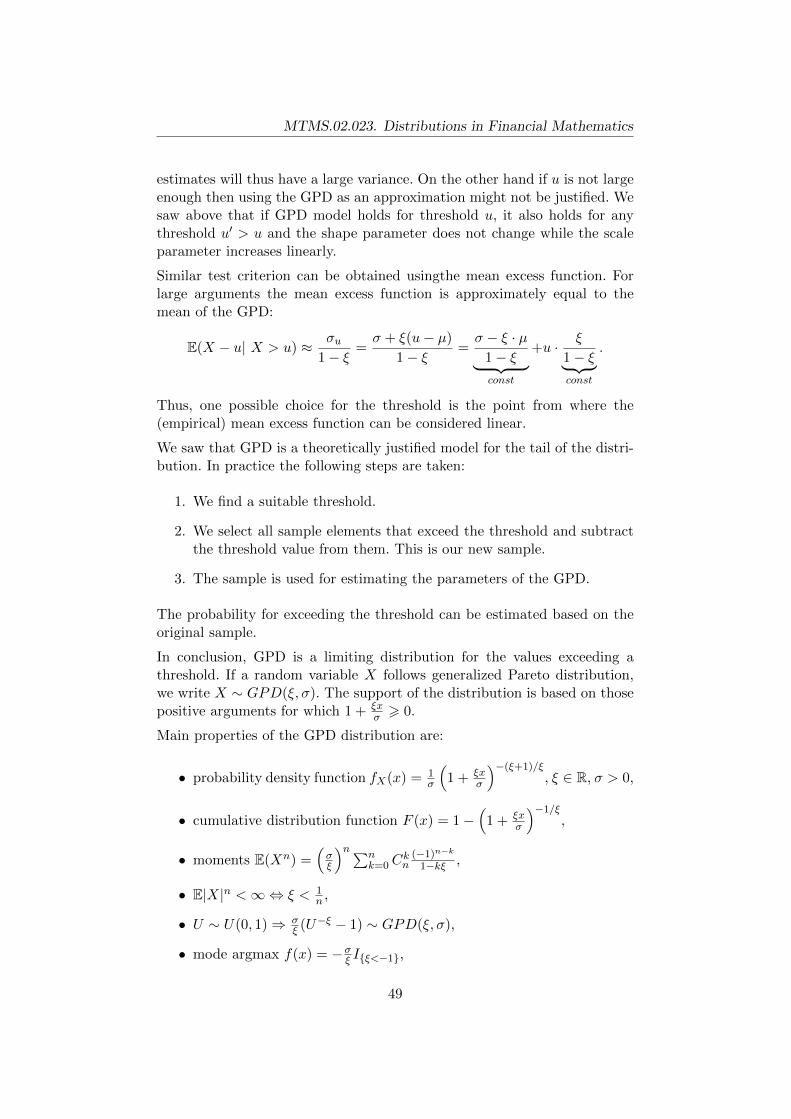
MTMS.02.023. Distributions in Financial Mathematics
estimates will thus have a large variance. On the other hand if u is not largeenough then using the GPD as an approximation might not be justified. Wesaw above that if GPD model holds for threshold u, it also holds for anythreshold u′ > u and the shape parameter does not change while the scaleparameter increases linearly.
Similar test criterion can be obtained usingthe mean excess function. Forlarge arguments the mean excess function is approximately equal to themean of the GPD:
E(X − u| X > u) ≈ σu1− ξ
=σ + ξ(u− µ)
1− ξ=σ − ξ · µ
1− ξ︸ ︷︷ ︸const
+u · ξ
1− ξ︸ ︷︷ ︸const
.
Thus, one possible choice for the threshold is the point from where the(empirical) mean excess function can be considered linear.
We saw that GPD is a theoretically justified model for the tail of the distri-bution. In practice the following steps are taken:
1. We find a suitable threshold.
2. We select all sample elements that exceed the threshold and subtractthe threshold value from them. This is our new sample.
3. The sample is used for estimating the parameters of the GPD.
The probability for exceeding the threshold can be estimated based on theoriginal sample.
In conclusion, GPD is a limiting distribution for the values exceeding athreshold. If a random variable X follows generalized Pareto distribution,we write X ∼ GPD(ξ, σ). The support of the distribution is based on thosepositive arguments for which 1 + ξx
σ > 0.
Main properties of the GPD distribution are:
• probability density function fX(x) = 1σ
(1 + ξx
σ
)−(ξ+1)/ξ, ξ ∈ R, σ > 0,
• cumulative distribution function F (x) = 1−(
1 + ξxσ
)−1/ξ,
• moments E(Xn) =(σξ
)n∑nk=0C
kn
(−1)n−k
1−kξ ,
• E|X|n <∞⇔ ξ < 1n ,
• U ∼ U(0, 1)⇒ σξ (U−ξ − 1) ∼ GPD(ξ, σ),
• mode argmax f(x) = −σξ I{ξ<−1},
49
MTMS.02.023. Distributions in Financial Mathematics
0 2 4 6 8 10
0.0
0.2
0.4
0.6
0.8
1.0
x
f(x)
GPD(1,1)GPD(−0.5,1)GPD(0,1)
Figure 27: The probability density function of GPD for different parametervalue combinations
• median med X = σ 2ξ−1ξ .
Home assignment 20. In what way does the GPD generalize the Paretodistribution?
50
MTMS.02.023. Distributions in Financial Mathematics
10 Stable distributions
Definition 10.1. We say that a random variable is stable (or has a stabledistribution) if for the cumulative distribution function F (x) and any n ∈ Nthere exist constants an > 0 and bn ∈ R such that for all x it holds that
F ∗n(x) = F (anx+ bn).
This is property is known as sum stability – sum of the random variables isstill in the same class.
We can conclude that if we have iid random variables X,X1, . . . , Xn and ifwe denote Sn = X1 + . . .+Xn, then for every positive integer n we have
Sn − bnan
d= X,
meaning that stable distributions are a limit distribution for normed sums.As it was with max-stable distributions, it turns out that this is the onlyclass of distributions appearing as a limit. Obviously, the most well knowndistribution belonging to this class is normal distribution.
The class has 4 parameters, the most important of them is the one thatdetermines the heaviness (actually the lightness) of the tails α ∈ (0, 2].The skewness parameter β ∈ [−1, 1] is also important. Scale and locationparameters are respectively γ and δ. Even though all stable distributions arecontinuous, only three combinations of (α,β) allow us to write an analyticdensity:
• α = 2, β = 0 gives us the normal distribution,
• α = 1, β = 0 gives us the Cauchy distribution, and
• α = 1/2, β = 1 is the Levy distribution.
In other cases one has to deal with the characteristic function.
Standard stable distribution (γ = 1 and δ = 0) has a characteristic function:
ϕ(t) =
{exp{−|t|α[1− iβ tan
(πα2
)sgn(t)]}, α 6= 1
exp{−|t|[1 + iβ 2π sgn(t) log |t|]}, α = 1.
51

MTMS.02.023. Distributions in Financial Mathematics
−4 −2 0 2 4
0.0
0.2
0.4
0.6
0.8
1.0
x
f(x)
S(2,0)S(1.5,0)S(1,0)S(0.5,0)
Figure 28: The effect of the shape parameter α to the tails of the stabledistribution
The larger the β the more heavy the right tail is compared to the left tail (andvice versa). We can see from the characteristic function that if X ∼ S(α, β)and Y ∼ S(α,−β), then X and −Y have the same distribution.
−10 −5 0 5 10
0.0
0.1
0.2
0.3
0.4
0.5
x
f(x)
S(1,0)S(1,0.5)S(1,1)
Figure 29: Effect of the skewness parameter β to the tails of the stabledistribution
52
MTMS.02.023. Distributions in Financial Mathematics
Main characteristics of a stable distribution are:
• probability density function and cumulative distribution function arenot analytically expressible (except for some parameter values),
• mean EX = δ, if α > 1, otherwise undefined,
• variance V arX = 2γ2, if α = 2, otherwise undefined,
• higher moments are undefined,
• median med X = δ if β = 0, otherwise not analytically expressible,
• mode argmax f(x) = δ if β = 0, otherwise not analytically expressible,
• moment generating function is undefined,
• skewness is 0 if α = 2, otherwise undefined.
Let us now consider an important limit theorem, which is actually the gener-alization of the CLT. The latter requires finite variance, as we know. We nowgeneralize the class of possible limit distributions and drop this requirement.
Theorem 10.1. The class of stable (non-degenerate) distributions coincideswith the class of all possible (non-degenerate) limit distributions for (properlynormalized and centered) sums of iid random variables.
In other words, if a distribution is stable, then it is a limit distributionfor sums of iid random variables. Moreover, it is the only possible limitdistribution for such sums.
We say that a distribution F is in the domain of attraction of an α-stabledistribution if a stable distribution with shape parameter α is a possible limitof the (normed) sum of iid F distributed random variables. Thus all finite-variance distributions (random variables) are in the domain of attraction ofa 2-stable distribution (normal distribution).
We know that when the variance is finite then the normalizing constantscan be represented using the mean and standard deviation. This is out ofthe question when the second moment does not exist. Actually it is worthnoticing that when normal distribution is the limit then an has the formn1/2C. Unfortunately, it is not as simple as selecting an in the form of nCwhen there is finite mean.
More precisely, (the Marcinkiewicz-Zygmund) law of large numbers statesthat if and only if E(X)p < ∞ for some p ∈ (0, 2), then for some b almostsurely
Sn − b · nn1/p
→ 0.
53
MTMS.02.023. Distributions in Financial Mathematics
But if E(X)p =∞ for some p ∈ (0, 2) then for every a almost surely
lim supn→∞
Sn − b · nn1/p
=∞.
So, roughly speaking, if we want a non-degenerate distribution then thescaling constant should be just of a lower order than the inverse of the rankof the last existing moment. So if E(X)p < ∞ if and only if p < 1, thenthe inverses of the existing moments form (1,∞) and we would expect thesuitable scaling constant to be of order n (too low order would probablycause too large a variance and the limit would not exist).
Definition 10.2. We say that a function f is slowly varying if for everyt > 0 we have that f(tx)/f(x)→ 1 when x→∞.
So, for example, a constant function and a logarithm function are slowlyvarying functions.
If a random variable X is in the domain of attraction of an α-stable distri-bution, we can choose the centering constant bn = E(X)n when α > 1 andbn = 0 otherwise. The scaling constant has the form
an = n1/αL(n),
where L is a suitable slowly varying function.
54

MTMS.02.023. Distributions in Financial Mathematics
11 Geometric stable distributions
In real life there are many random entities that are dependent on smallimpacts. We can imagine that a stock prices (or price change) is a result ofmany small factors and each factor has a small effect. The number of thesesmall factors is probably not constant (when we compare days). Thus thenumber of random variables summed up should also be random. This leadsus to geometric stable distributions.
Let a random variable N have a geometric distribution with parameter p ∈(0, 1), i.e for each positive integer k we have
P(N = k) = p(1− p)k−1.
Definition 11.1 (Geometric stability). We say that a random variable Yis geometric stable if for some sequence of iid random variables X1, X2, . . .that is also independent of N , there exist normalizing constants ap > 0 andbp ∈ R such that
N∑i=1
Xi − bpap
d→ Y
in the process p→ 0.
Let us look at standard exponential random variables in the role of thesummands. Let p ∈ (0, 1) and
Y = pN∑i=1
Xi, (11.1)
whereN is geometrically distributed as before. So we are interested in findinga limit distribution (or the corresponding density function) of a geometricsum. Let us denote S =
∑Ni=1Xi. Then, by (11.1), we have
P(Y 6 x) = P(S 6
x
p
),
which for densities implies
fY (x) =1
pfS
(x
p
).
Notice also that by the construction, the sum S is a discrete mixture, andfor any fixed k, the conditional distribution of S given N = k is gammadistribution (as it is sum of independent exponentials) with parameters k
55

MTMS.02.023. Distributions in Financial Mathematics
and 1. Thus, we can retrieve the marginal density of Y through conditionaldistribution of S|N and marginal distribution of N :
fY (x) =1
p
∞∑k=1
fS|N=k
(x
p
)fN (k)
=1
p
∞∑k=1
(xp
)k−1e−x/p
Γ(k)p(1− p)k−1
= e−x/p∞∑k=1
(1− p)k−1(xp
)k−1
(k − 1)!,
where we recognize the Taylor expansion of the exponential function andthus obtain
fY (x) = e−x/pe(1−p)x/p = e−x
which means that the limit distribution is also standard exponential (andwe even did not have to consider p → 0) and exponential distribution isgeometric stable.
In a more general case Renyi theorem states that if positive summands havefinite mean then the normalized sum
pN∑i=1
Xi
always yields the exponential distribution as a limit in the process p→ 0. Ifthe summands are symmetrical and have finite variance then the sum
√p
N∑i=1
Xi
has a Laplace (distribution) limit.
So very often either exponential or Laplace distribution is the limit. But if weloosen the assumptions then the set of possible limit distributions expands.Let us still consider the case bp = 0, i.e. the sum has the form
Y =1
ap
N∑i=1
Xi,
in the process p → 0. If the summands are positive but we do not assumefinite variance then the Mittag-Leffler class of distributions arises as the limitset. If the summands are symmetrical (but variance not necessarily finite)then the Linnik class of distributions arises as the limit set.
56
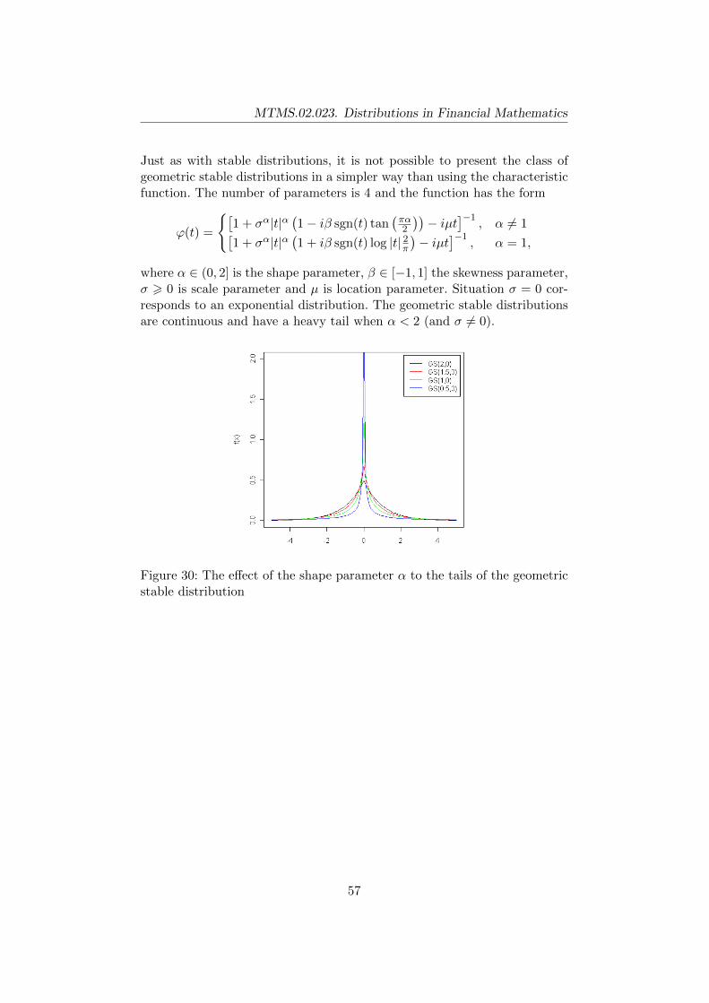
MTMS.02.023. Distributions in Financial Mathematics
Just as with stable distributions, it is not possible to present the class ofgeometric stable distributions in a simpler way than using the characteristicfunction. The number of parameters is 4 and the function has the form
ϕ(t) =
{[1 + σα|t|α
(1− iβ sgn(t) tan
(πα2
))− iµt
]−1, α 6= 1[
1 + σα|t|α(1 + iβ sgn(t) log |t| 2π
)− iµt
]−1, α = 1,
where α ∈ (0, 2] is the shape parameter, β ∈ [−1, 1] the skewness parameter,σ > 0 is scale parameter and µ is location parameter. Situation σ = 0 cor-responds to an exponential distribution. The geometric stable distributionsare continuous and have a heavy tail when α < 2 (and σ 6= 0).
Figure 30: The effect of the shape parameter α to the tails of the geometricstable distribution
57

MTMS.02.023. Distributions in Financial Mathematics
Figure 31: The effect of the skewness parameter β to the tails of the geometricstable distribution
If an analytic probability density function does not exist then the use of MLfor parameter estimation is not straightforward (a grid method would bepretty imprecise and time consuming). An empirical characteristic function
1
n
n∑i=1
eitxi ,
is constructed and then the real and imaginary parts are equated (for theo-retical and empirical functions) to form the equations. Different (arbitrary)values of tj are used for this. Obviously, the choice of the values tj is still aproblem to be addressed.
Alternative approach for finding parameters is to use the method of (non-integer) moments
This method is based on fact that for a geometric stable distribution, themoments E|X|p are finite if p < α
Then, the moments matching can be done through a 2-step process:
• detect the value of α (using the tools described previously)
• choose four constants less than that estimated value to form the equa-tions.
58

MTMS.02.023. Distributions in Financial Mathematics
12 Goodness of fit of a model
Any fitting problem with different candidate models sooner or later meetsthe question of how to measure which candidate is better, and, finally, whichmodel should we choose. When one of the candidates is a special case ofthe other (nested models) then this is quite straightforward. If not thenmore thought is required. Likelihood function which is an intuitive startingpoint for comparing two models (especially when ML was used for parameterestimation) cannot be used directly.
12.1 Kolmogorov-Smirnov test
Let us assume that the distribution function F of a theoretical candidatedistribution is continuous. To first answer whether the data fits the distri-bution a graphical method is used. QQ-plot is one of the options. Whendrawing the QQ-plot the role of the inverse cumulative distribution func-tion is assumed by F−1. In practice, the theoretical candidate is rarely fullyspecified. It is common to take a candidate from a specified class of distribu-tions, but the parameters need to be estimated (from data). Let us denotethe corresponding distribution by F ∗.
Let Fn be the empirical cumulative distribution function. Clearly the func-tion
D(x) := |Fn(x)− F (x)|
measures the goodness of fit. Thus the graph of this function is a possibletool for our purposes.
But we can also quantify the fit quality. For example, we might postulatethe null hypothesis that the data comes from a known distribution F andthe alternative hypothesis is thus the negation of this statement – data doesnot come from F . To test this hypothesis it is wise to make use of functionD(x).
Kolmogorov-Smirnov test is based on the statistic
supx|Fn(x)− F (x)|,
the value of which is compared with a critical value. If it is exceeded thenthe null hypothesis is rejected. Although it might seem to be complicated,it is in fact easy to calculate the value of the statistic. This is so becausethe cumulative distribution function F (x) is continuous and the empiricalcumulative distribution function is a step function. This means that thesupremum of D(x) is always attained at some sample element or ”just beforeit”.
59

MTMS.02.023. Distributions in Financial Mathematics
There is one thing that is very often overlooked – the definition of F mustbe independent from the sample. This means that we cannot use F ∗ in therole of F , because the parameters of it are estimated from the sample. If wedo it then the test no longer works properly – null hypothesis is often notrejected (when it should be) and the power of the test is thus reduced.
The solution out of this is the splitting of the sample – first part is usedfor parameter estimation (i.e. finding F ) and the other part is used forconstructing Fn.
Let us illustrate the previous fact with a simulation. First let us generate1000 samples, each with size n = 100, from standard normal distributionand each time find the Kolmogorov-Smirnov test statistic using the standardnormal distribution in the role of F as well. For the second case we use thesame generation rule but in the role of F we use a normal distribution,parameters of which are estimated using the same sample. For the thirdcase again we use the same generation rule but the parameters are estimatedusing the first half of the sample (and this way F is chosen). The secondhalf is used for constructing Fn.
From the first experiment we get that the 0.95 quantile is 0.133 (this is thecritical value for this sample size because the test is distribution free andbased only on the values of the cumulative distribution function). But in thesecond experiment this critical value is very rarely exceeded even though thecandidate F is always wrong (even if just a little). In the third experimentthe situation is more plausible – about half the simulations lead to rejectingthe null hypothesis (as it should be). The fact that this does not happenmore often is due to the power of the test.
0.05 0.10 0.15
050
100
150
0.04 0.06 0.08 0.10 0.12
050
100
150
200
250
0.05 0.15 0.25
050
100
150
Figure 32: Distribution of the Kolmogorov-Smirnov statistic for differentusage scenarios
60

MTMS.02.023. Distributions in Financial Mathematics
12.2 Anderson-Darling test
Anderson-Darling test also makes use of D(x), but extra weight is placed onthe tails. Test statistic is formed as an integral
n
∫(Fn(x)− F (x))2
F (x)F (x)f(x)dx,
where the integral is over the full support of the distribution and f(x) isthe probability density function corresponding to F . So essentially this is anaverage of D2(x), but the weights are not uniform – large and small argu-ments are up-weighted. On the other hand this is quite reasonable becauseas every cumulative distribution function begins with zero and ends withone and thus otherwise the difference near the tails would be small. For thistest it also holds that F should be determined independently from the data.
12.3 Likelihood ratio test
Suppose now that we have 2 candidate models and A is a special case of B– B simplifies to A when we fix one of its parameters (we can just say thatA is a simpler model than B). Then the value of the likelihood function forA (lets call it L0) cannot be larger than the value for B (lets call it L1),where in both cases ML is used. The ratio of the two values is connected toχ2 distribution. The test statistic
2 ln
(L1
L0
)is approximately χ2-distributed where the degrees of freedom is equal to thenumber of extra parameters that B has. Null hypothesis is thus that A isgood enough and alternative hypothesis is that B is considerably better.
Remark 12.1. We can also use the test so that we fix, e.g., the mean ofthe distribution, and even if this depends on several parameters then thenumber of free parameters for A is one less than for B. Even though none ofthe parameters is strictly fixed, we can still use the likelihood ratio statistic.
In a situation where one model is not the extension of other, the likelihoodratio cannot be properly used.
Let us rewrite the likelihood ratio and look for possible generalizations. Letcr,α be the 1-α-quantile of the distribution χ2(r). Then the likelihood ratiostatistic tells us to use a more complicated model (with r extra parameters)if
61
MTMS.02.023. Distributions in Financial Mathematics
lnL1 > lnL0 +cr,α2,
where L1 is the likelihood function value for the more complicated modeland L0 is the likelihood function value for the simpler model. Thus we seethat there is also term that can be viewed as penalty – one extra parameterrequires that the log-likelihood should increase by at least c1,α/2.
This argumentation leads to the general idea of information criteria – wecompare the likelihood of different models and apply certain penalty functionto a more complex model.
12.4 Information criteria. Akaike information criterion (AIC)
Information criteria (which are also based on log-likelihood) are also toolsfor measuring the goodness of a model. The most well-known of them isAkaike information criterion, which is a statistic defined by
AIC = −2 ln(maximum likelihood) + 2p,
where p is the number of parameters in a model under consideration.
So, AIC measures the goodness of fit as certain tradeoff between two com-ponents:
• goodness of fit (measured by the log-likelihood),
• model complexity (measured by the number of parameters p).
Information criteria can also take the sample size into account.
Bayesian IC (aka Schwarz IC) is calculated as
BIC = −2 lnL+ p lnn,
This means that when there are r extra parameters and the sample size isn then we should reduce the log-likelihood by (r/2) lnn, or, in other words,each additional parameter is deemed worthy when the log-likelihood is in-creased by 0.5 lnn. When this is not the case then a simpler model shouldbe preferred.
The corrected AIC says that we should pick a model for which
AICc = AIC +2p(p+ 1)
n− p− 1= −2 lnL+ 2p+
2p(p+ 1)
n− p− 1
is smallest. One should also note that when the number of parameters isequal then the decision is essentially based on the likelihood function value.
62
MTMS.02.023. Distributions in Financial Mathematics
13 Conclusion
Let us now try to summarize what we have learned.
1. What is our goal? Modelling the distribution is typically not the ul-timate task but only a useful (and necessary) step to answer somequestion. This means that sometimes we do not need to model thewhole distribution, perhaps only some part of it. So e.g. when we areinterested in predicting the 0.99-quantile then it probably makes senseto just fit a GPD on the tail of the distribution and leave out the mainpart.
2. Are our data realizations of iid random variables? We have consid-ered the test of records. We can also look at the signs of consecutiveobservations and other non-parametric tests. Also squaring the obser-vations can be useful to study the correlation (and possibly rule outindependence). We could also look at the behavior of the median (orsome other quantile) in the sub-samples. Tests based on the mean areoften not useful in the heavy-tailed data context.
Some transformation might help us (log-returns seem less correlatedthan stock prices).
Sometimes it can happen that we are not interested in independence– perhaps we only do wish to model the distribution. Then we havea situation similar to a Markov chain, where neighboring observationsare clearly correlated but still are realizations from the distributionthat we are interested in. (e.g. the Gibbs sampler). Then ”obtainingindependence” is also similar – we thin our observations by leaving out,say, nine out of ten and only retaining every tenth observation. Thisis of course very costly.
3. Modeling usually begins with the selection of the model class. We mustponder whether there is a clear basis to prefer one distribution to an-other (e.g. somehow it is known beforehand that a Pareto distributioncan fit but Weibull definitely does not fit). Here the ratio of maximumand sum might help us. When we don’t find a suitable candidate thenit might be necessary to make one up, but this can lead to a multitudeof complications. Sometimes the lack of data can also limit our choicefor distributions. And if we are not certain that we have heavy-taileddata then this should also be tested for by visualizing the mean excessfunction or creating a suitable QQ-plot.
4. Depending on the class of distributions chosen different parameter es-timation methods can be used. The best situation is the one where dif-ferent estimation methods lead to similar parameter estimates. Even
63

MTMS.02.023. Distributions in Financial Mathematics
though it is generally reasonable to ask for good asymptotic proper-ties, we must realize that e.g. the consistency of an estimator doesnot guarantee us anything beneficial when we have a moderate-sizedsample.
5. Sometimes it may turn out that a model which seemed reasonabledoes not give us a good fit. In this case the model must often be aban-doned and the process must start over. Shortcomings of the modelcan sometimes be detected using the kernel density estimate for com-parison (or perhaps the QQ-plot). Cross-validation or just separatetraining and test data are useful. This last scenario allows us to usethe Kolmogorov-Smirnov test.
6. When we do not have one and only model in consideration and thegoodness of a model is simply based on fit there still might be the desireto arrive at a single (final) model. Model selection is usually handledusing information criteria. The question of how large a difference inthose values is large enough to rule out worse models is still a criticalquestion.
7. When we have a parametric model then usually answering any partic-ular questions using this model is quite straightforward. Sometimes asensitivity analysis might be required (to show how much the changesin parameter estimates affect the answer to our question). This is alsothe case when our modelling process leads to several competing mod-els.
64