Distribution of Downward Flux in Unsaturated …downward flow should be anticipated in heterogeneous...

E *1 *~f OV% Wi -,t M alef

DISTRIBUTION OF DOWNWARD FLUX INUNSATURATED HETEROGENEOUS HYDROGEOLOGIC ENVIRONMENTS

by

ProfessorGeorge Bloomsburgof Agricultural Engineering

Roy E. WilliamsProfessor of Hydrogeology

James OsienskyAssociate Professor of Hydrogeology

University of IdahoMoscow, Idaho 83843

and

All Are Associates ofWilliams and Associates, Inc.

P.O. Box 48Viola, Idaho 83872

April 1988

O 8 7290278--8EO72"2-mPDR WMRES EECWILAD-1020 PDC

---1

I

DISTRIBUTION OF DOWNWARD FLUX INUNSATURATED HETEROGENEOUS HYDROGEOLOGIC ENVIRONMENTS

Abstract

The finite element computer program UNSAT2 was used to investigate

the horizontal distribution of unsaturated downward flux in porous tuff

as a function of hydrogeologic heterogeneities under two different

recharge rates. The distribution of downward flux is important because of

its influence on groundwater travel time at a potential geologic

repository for high-level radioactive wastes. Hydraulic properties of

the Topopah Spring Member of the Paentbrush Tuff Formation at Yucca

Mountain, Nevada, as reported by Peters et al. (1984) were selected for

use in the eight simulations that were conducted. All simulations were

run essentially to steady state. The simulations show that: 1)

heterogeneities in an isotropic porous rock matrix will cause downward

flux to be distributed nonuniformly; 2) zones in which saturated matrix

hydraulic conductivity is less than the downward flux tend to develop

positive pressures which may cause flow into fractures if they exist; 3)

one-dimensional analysis of vertical flow in the unsaturated zone is

insufficient to ensure that fracture flow does not occur even if the true

magnitude of vertical flux is known; and 4) the true spatial distribution

of hydraulic conductivity above the regional water table must be

determined in order to obtain the true spatial distribution of downward

flux; this analysis assumed constant spatial and temporal distribution

of recharge for each simulation but the difference among simulations

verify the fact that changing recharge rates also play a significant role

in the distribution of downward flux due to the influence of recharge

3

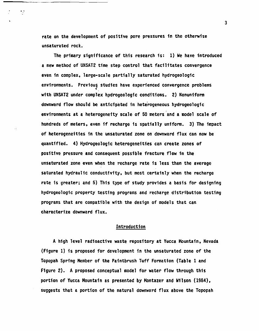
rate on the development of positive pore pressures in the otherwise

unsaturated rock.

The primary significance of this research is: 1) We have introduced

a new method of UNSAT2 time step control that facilitates convergence

even in complex, large-scale partially saturated hydrogeologic

environments. Previoul studies have experienced convergence problems

with UNSAT2 under complex hydrogeologic conditions. 2) Nonuniform

downward flow should be anticipated in heterogeneous hydrogeologic

environments at a heterogeneity scale of 50 meters and a model scale of

hundreds of meters, even if recharge is spatially uniform. 3) The impact

of heterogeneities in the unsaturated zone on downward flux can now be

quantified. 4) Hydrogeologic heterogeneities can create zones of

positive pressure and consequent possible fracture flow in the

unsaturated zone even when the recharge rate is less than the average

saturated hydraulic conductivity, but most certainly when the recharge

rate is greater; and 5) This type of study provides a basis for designing

hydrogeologic property testing programs and recharge distribution testing

programs that are compatible with the design of models that can

characterize downward flux.

Introduction

A high level radioactive waste repository at Yucca Mountain, Nevada

(Figure 1) is proposed for development in the unsaturated zone of the

Topopah Spring Member of the Paintbrush Tuff Formation (Table 1 and

Figure 2). A proposed conceptual model for water flow through this

portion of Yucca Mountain as presented by Montazer and Wilson (1984),

suggests that a portion of the natural downward flux above the Topopah

4

SOUTHERN NEVADA

0 2 4kilometers l_

I

I

i1

z

0N

VEGAS* __ _II

l

- TENTATIVE LOCATION OFUNDERGROUND REPOSITORY

YUCCA MOUNTAIN SITE

Figure 1. Location of the site for a possible radioactive-waste repositoryat Yucca Mountain in southern Nevada; A-A' shows the location ofthe geologic cross section in figure 2 (modified after Sinnocket al., 1984).

.5

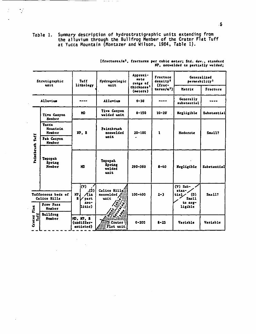
Table 1. Summary description of hydrostratigraphic units extending fromthe alluvium through the Bullfrog Member of the Crater Flat Tuffat Yucca Mountain (Montazer and Wilson, 1984, Table 1).

(frsctures/l, fractures per cubic meter; Std. dCv., standardNP. noovelded to partially welded;

Approei- Fracture Generalized

Strztigraphic Tuff Kydrogeologic mate densitys perceability'unit lithology unit raicnge of (frac-

0 Iwt es) tures/m3) fatri j Fracture(SC~~~~erearll

Alluvium ---- Alluvium 0-30 ---- tenerally ----substantial

3

S.c

o

3.a'

Ca6'

Tiva CanyonMember

YuccamountainMember

Pah CanyonMember

TopopahSprintMember

Tiva Canyonwelded unit 0-150 10-20 Negligible

PaintbrushNP, 8 convelded 20-100 I Moderate Small?

unit -

Topopab

M vdSprin 290-360 8-40 Negligible SubstantialweldeduniLt

Substantial

Tuffaceous beds ofCalico Hills

Prow Passso Member

B _ Bullfrog.. member

a_U

B

(v) ,f,(D)

Am/ part

litie)

MD, NP. B(undiffer-entiated)

_ - - - -_

Calico Hillh;nonwelded Al'

unit e s-

t CrsternFia t unl

100-400 2-3

(V) Sub- -I'stan-,

tisl e (D)

I to neg-ligible

Sa I 1?

I 4. 4. 4.

0-200 8-25 Variable Variable

__----- __

6

A'1500

zZ0, 1000

4

UI

500

4,;;. - Tentative7k m _ Repository-T Zone

SaturatedZone

Horizontal Scale

GM

Timber Mountain Tutf

Tiva Canyon Member. Paintbrush Tuft

Nonwelded Paintbrush Tuft

Topopah Spring Member. Paintbrush Tuft

Tuffaceous Beds of Calico Hills

Prow Pass Member. Crater flat Tuft

Bull Frog Member. Crater Flat Tuft

Tram Member. Crater Flat Tuft

0 0.2s 0.sokilometers

0.75

Figure 2. Geologic cross section of Yucca Mountain showing the tentativedepth of a possible repository in the Topopah Spring Member ofthe Paintbrush Tuff (Sinnock et al., 1984).

7

Spring Member is diverted around the site by "capillary barriers."

Montazer and Wilson assume that this diverted flux may flow laterally

under the influence of a *capillary barrier* toward structural features

at the edge of the repository but they provide no supportive information

such as modeling. Peters and Klavetter (1988) present a method of

viewing such a fractured geologic environment as a continuum. Sinnock

et al. (1986) assume on the other hand that the downward flux is

distributed uniformly in the horizontal plane. The evaluation of that

important assumption is a primary goal of this paper.

The unsaturated model for flow in the Topopah Spring Member used in

this study requires neither Ocapillary barriers," nor uniform

distribution of downward flux. This conceptual model includes spatially

varying hydraulic properties (heterogeneities) of the Topopah Spring tuff

and the consequent variations in horizontal distribution of downward

flux. Some of these heterogeneities may be envisioned as structural

features such as faults. Others may be produced by random (or nonrandom)

cooling processes that are not yet understood. All hydrogeologic

heterogeneities discussed herein as possible structural features are

treated as equivalent porous media. That is, the model does not simulate

flow in discrete fractures.

Objectives of Study

The objectives of this unsaturated flow modeling study are as

follows:

1. Quantify the effects that heterogeneous hydraulic properties have on

the horizontal distribution of downward flux under unsaturated

conditions in porous rock.

I * ,

8

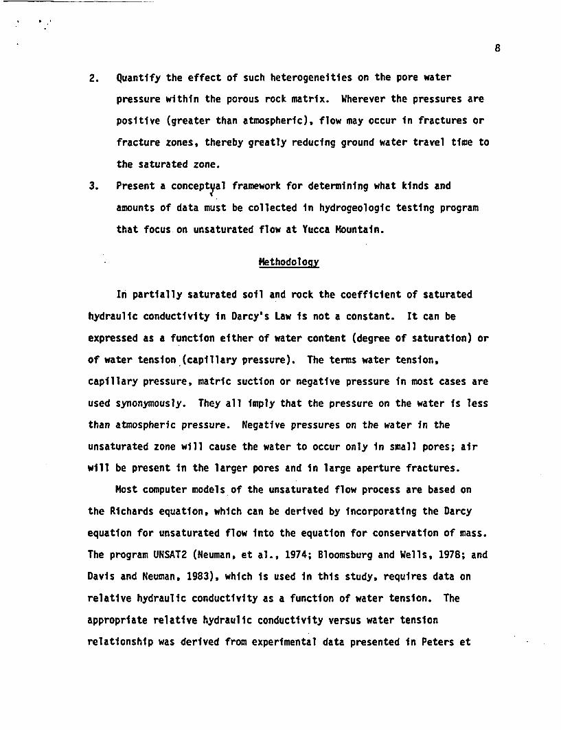
2. Quantify the effect of such heterogeneities on the pore water

pressure within the porous rock matrix. Wherever the pressures are

positive (greater than atmospheric), flow may occur in fractures or

fracture zones, thereby greatly reducing ground water travel time to

the saturated zone.

3. Present a conceptyal framework for determining what kinds and

amounts of data must be collected in hydrogeologic testing program

that focus on unsaturated flow at Yucca Mountain.

Methodology

In partially saturated soil and rock the coefficient of saturated

hydraulic conductivity in Darcy's Law is not a constant. It can be

expressed as a function either of water content (degree of saturation) or

of water tension (capillary pressure). The terms water tension,

capillary pressure, matric suction or negative pressure in most cases are

used synonymously. They all imply that the pressure on the water is less

than atmospheric pressure. Negative pressures on the water in the

unsaturated zone will cause the water to occur only in small pores; air

will be present in the larger pores and in large aperture fractures.

Most computer models of the unsaturated flow process are based on

the Richards equation, which can be derived by incorporating the Darcy

equation for unsaturated flow into the equation for conservation of mass.

The program UNSAT2 (Neuman, et al., 1974; Bloomsburg and Wells, 1978; and

Davis and Neuman, 1983), which is used in this study, requires data on

relative hydraulic conductivity as a function of water tension. The

appropriate relative hydraulic conductivity versus water tension

relationship was derived from experimental data presented in Peters et

9

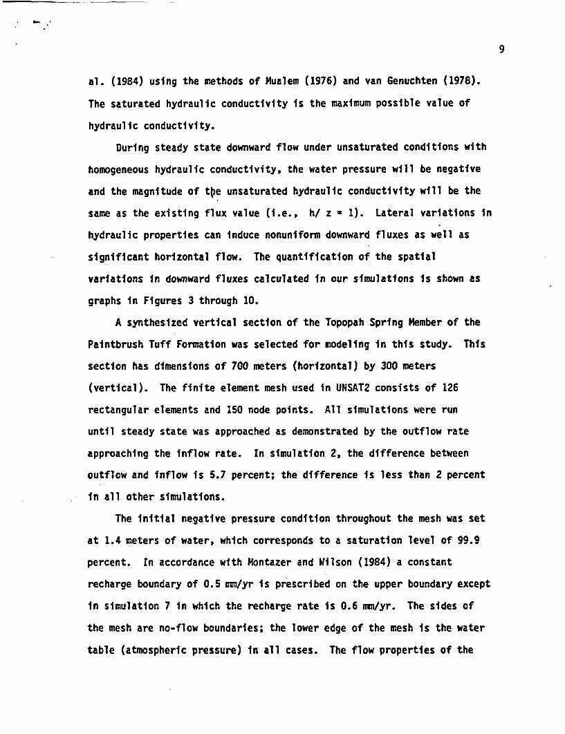
al. (1984) using the methods of Nualem (1976) and van Genuchten (1978).

The saturated hydraulic conductivity is the maximum possible value of

hydraulic conductivity.

During steady state downward flow under unsaturated conditions with

homogeneous hydraulic conductivity, the water pressure will be negative

and the magnitude of toe unsaturated hydraulic conductivity will be the

same as the existing flux value (i.e., h/ z = 1). Lateral variations in

hydraulic properties can induce nonuniform downward fluxes as well as

significant horizontal flow. The quantification of the spatial

variations in downward fluxes calculated in our simulations is shown as

graphs in Figures 3 through 10.

A synthesized vertical section of the Topopah Spring Member of the

Paintbrush Tuff Formation was selected for modeling in this study. This

section has dimensions of 700 meters (horizontal) by 300 meters

(vertical). The finite element mesh used in UNSAT2 consists of 126

rectangular elements and 150 node points. All simulations were run

until steady state was approached as demonstrated by the outflow rate

approaching the inflow rate. In simulation 2, the difference between

outflow and inflow is 5.7 percent; the difference is less than 2 percent

in all other simulations.

The initial negative pressure condition throughout the mesh was set

at 1.4 meters of water, which corresponds to a saturation level of 99.9

percent. In accordance with Montazer and Wilson (1984) a constant

recharge boundary of 0.5 mm/yr is prescribed on the upper boundary except

in simulation 7 in which the recharge rate is 0.6 mm/yr. The sides of

the mesh are no-flow boundaries; the lower edge of the mesh is the water

table (atmospheric pressure) in all cases. The flow properties of the

10

tuff were obtained from Peters et al. (1984). The values used are

derived from laboratory analysis of core hole samples obtained from

borehole G-4; however, samples from borehole GU-3 have comparable

properties. Relative permeability vs. pressure data were obtained from

Peters et al. (1984).

In the first simulation, the entire flow region is homogeneous and

isotropic with a saturated hydraulic conductivity of 0.601 mm/yr. This

value was obtained by Peters et al. (1984) by testing core sample G4-5;

it is approximately the geometric average of the measured values of

saturated hydraulic conductivity for the Topopah Spring Member. The

unsaturated permeability and soil moisture values are those reported by

Peters et al. (1984) for this sample of rock. This porous medium is

referred to herein as Raverage conductivity rock.

The remaining simulations have this average conductivity of 0.601

mm/yr assigned to the majority of the isotropic elements in the mesh.

However, in cases 2 through 8 various arrangements of elements are

assigned either a high conductivity (1.26 mm/yr) or low conductivity

(0.211 mm/yr). These two values are referred to herein as 'high

conductivity and glow conductivity rock. The saturated conductivities

reported by Peters et al. (1984) for samples from the two boreholes (G4

and GU-3) range from 0.047 to 14.19 mm/yr; therefore, the values used

herein do not reflect the full range of values known at this time. We

elected subjectively not to use the extreme values on either end of the

spectrum.

Detailed hydrogeologic heterogeneity has not been mapped in the

Topopah spring Member, but several faults have been mapped. The volcanic

tuff in the Topopah Spring Member consists of a compound cooling unit

11

composed of as many as four separate ash-flow sheets (U.S. DOE, 1986);

consequently even without structures such as faults the Topopah Spring

Member could display wide variations in all hydraulic properties because

of variations in flow conditions at the time of deposition and because of

variations in the rate of cooling of the ash.

A table of random numbers was used to select the locations of the

high and low conductivity elements in Cases 6, 7 and 8; even so, the

resulting distribution of hydraulic properties among the elements shows

some spatial correlation (i.e., some of the high or low conductivity

elements are clustered). Detailed characterization is needed to identify

the actual correlation scale.

The scale of variation of flow properties will not be known until

the Topopah Spring Member is characterized in great detail. The scale of

variation of hydrogeologic properties in our simulations is on the order

of 50 meters (the width of each element). Diagonal, vertical and

urandomu arrangements of the low and high conductivity elements were used

in the various simulations. A more detailed description of the various

simulations conducted in this study follows.

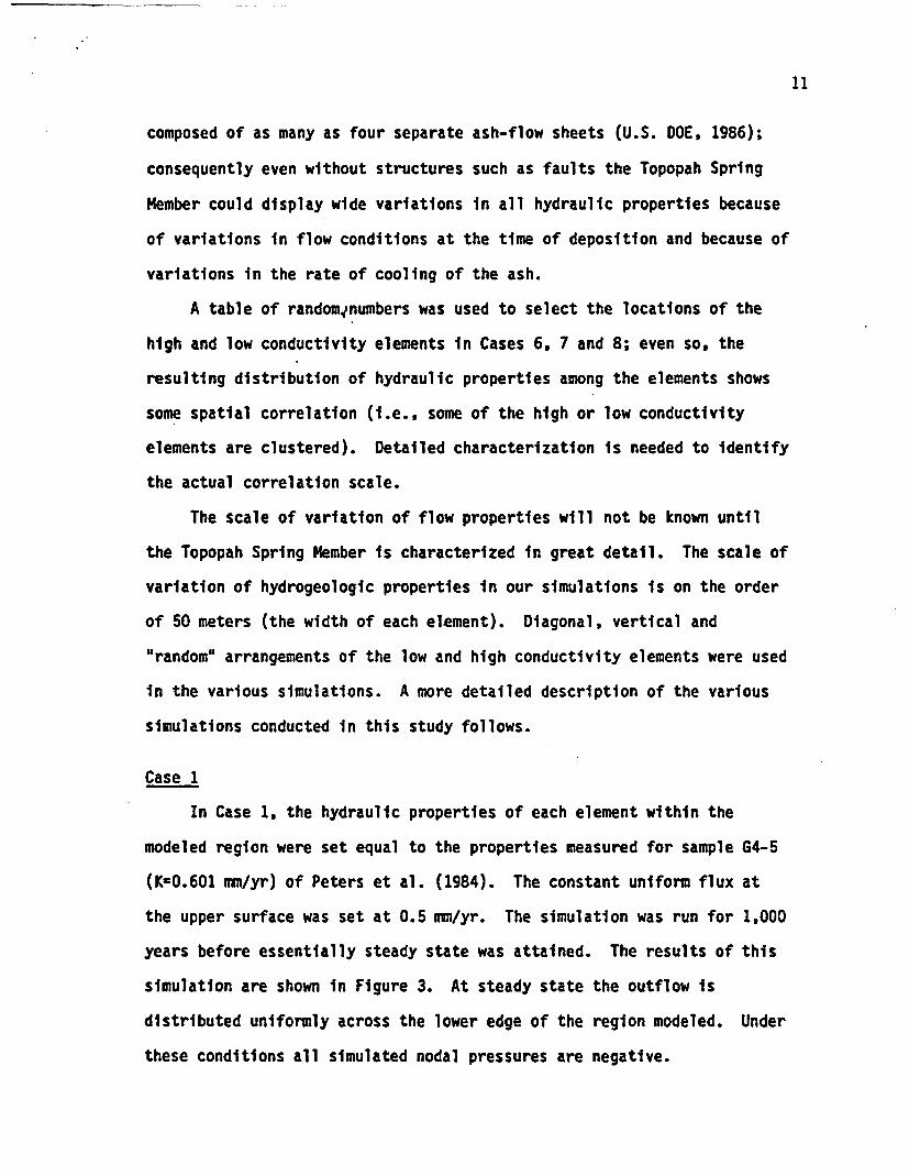
Case 1

In Case 1, the hydraulic properties of each element within the

modeled region were set equal to the properties measured for sample G4-5

(K=0.601 mm/yr) of Peters et al. (1984). The constant uniform flux at

the upper surface was set at 0.5 mm/yr. The simulation was run for 1,000

years before essentially steady state was attained. The results of this

simulation are shown in Figure 3. At steady state the outflow is

distributed uniformly across the lower edge of the region modeled. Under

these conditions all simulated nodal pressures are negative.

12

NODE NUMBERSELEMENT NUMBERS

/024

O0 4 700 meters /50

U0

0

E00

rn

-----I --1 -I- -- - -I24 60, 96

14 32 50 68 86 104 122

4 40 76 112

0-- I I Ind

r.

*.21-

- j

U&.

4i-

- -- - - - - - - - a…- -

.61-

.81-

.

II U'*SIMULATED AND AVERAGE FLUX - -

Figure 3. Finite element mesh and computed fluxes at bottom of meshfor Case 1; homogeneous distribution of hydraulicconductivity. All nodal pressures computed by the modelare negative.

Al

13

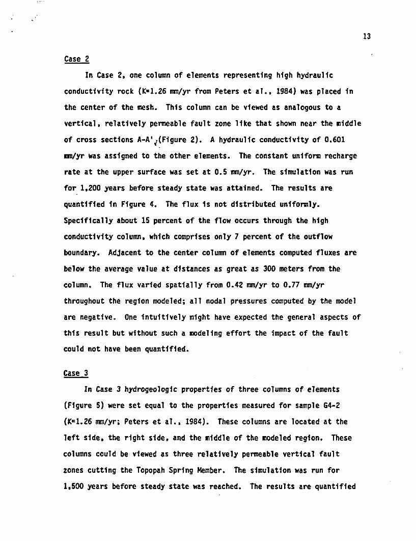
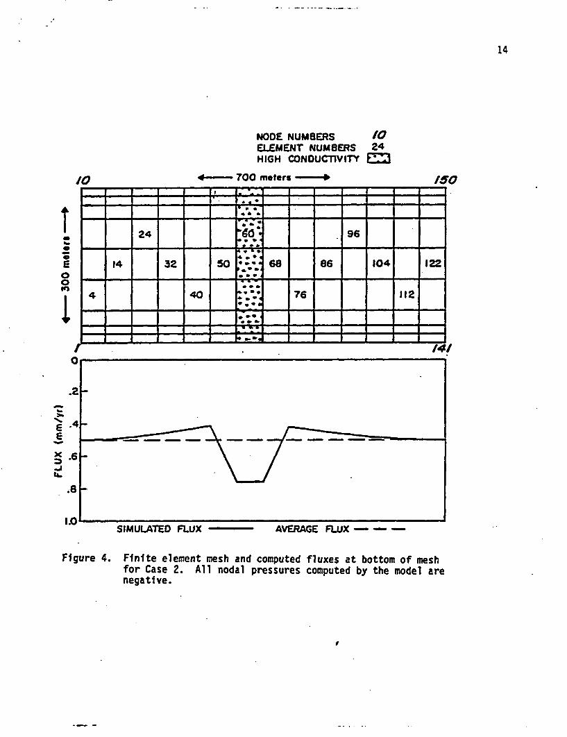
Case 2

In Case 2, one column of elements representing high hydraulic

conductivity rock (K-1.26 mm/yr from Peters et al., 1984) was placed in

the center of the mesh. This column can be viewed as analogous to a

vertical, relatively permeable fault zone like that shown near the middle

of cross sections A-A',(Figure 2). A hydraulic conductivity of 0.601

mm/yr was assigned to the other elements. The constant uniform recharge

rate at the upper surface was set at 0.5 mm/yr. The simulation was run

for 1,200 years before steady state was attained. The results are

quantified in Figure 4. The flux is not distributed uniformly.

Specifically about 15 percent of the flow occurs through the high

conductivity column, which comprises only 7 percent of the outflow

boundary. Adjacent to the center column of elements computed fluxes are

below the average value at distances as great as 300 meters from the

column. The flux varied spatially from 0.42 mm/yr to 0.77 mm/yr

throughout the region modeled; all nodal pressures computed by the model

are negative. One intuitively might have expected the general aspects of

this result but without such a modeling effort the impact of the fault

could not have been quantified.

Case 3

In Case 3 hydrogeologic properties of three columns of elements

(Figure 5) were set equal to the properties measured for sample G4-2

(K=1.26 mm/yr; Peters et al., 1984). These columns are located at the

left side, the right side, and the middle of the modeled region. These

columns could be viewed as three relatively permeable vertical fault

zones cutting the Topopah Spring Member. The simulation was run for

1,500 years before steady state was reached. The results are quantified

14

NODE NUMBERSELEMENT NUMBERSHIGH CONDUCTIVITY

/024

4- 7O0 meters -*

00in

XI

:0.

E-J

I-j

1.SIMULATED FLUX - AVERAGE FLUX - - -

Figure 4. Finite element mesh and computedfor Case 2. All nodal pressuresnegative.

fluxes at bottom of meshcomputed by the model are

V

15


/024

4- 700 meters b

0

0

S-J

=IL

1.SIMULATED FLUX

Figure 5. Finite element mesh and computed fluxes at bottom of meshfor Case 3. All nodal pressures computed by the model arenegative.

16

in Figure 5. The flux through the high conductivity columns is about

twice the average flux. About 42 percent of the flow moved through 21

percent of the area. The flux values vary spatially from 0.36 mm/yr to 1

mm/yr throughout the region modeled; all nodal pressures computed by the

model continue to be negative.

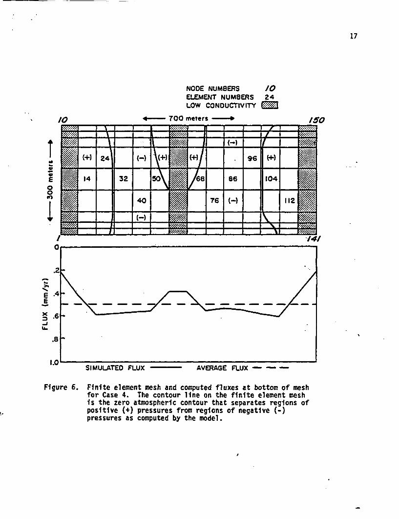
Case 4

This simulation was designed to test the effects of flow through a

medium with columns of rock that display less than average hydraulic

conductivity (K-0.211 umnyr). This value of hydraulic conductivity was

obtained for sample G4-1F of Peters et al. (1984). The left, right, and

center columns of elements inserted into the model of Case 4 represent

rock with this average value of conductivity (Figure 6). These three

columns of relatively low hydraulic conductivity elements could be viewed

as three fault zones that contain relatively low unsaturated hydraulic

conductivity gouge (e.g., Figure 2). The simulation was run for 1,000

years prior to reaching steady state. The results are quantified in

Figure 6. The flux values vary spatially from 0.21 nm/yr to 0.6 mm/yr

throughout the region modeled. Most of the elements that contain the

lower conductivity rock, as well as many of the neighboring node points,

developed positive pressures by the time steady state was reached. The

areas of positive pressure also are shown in Figure 6. This result would

not have been expected.

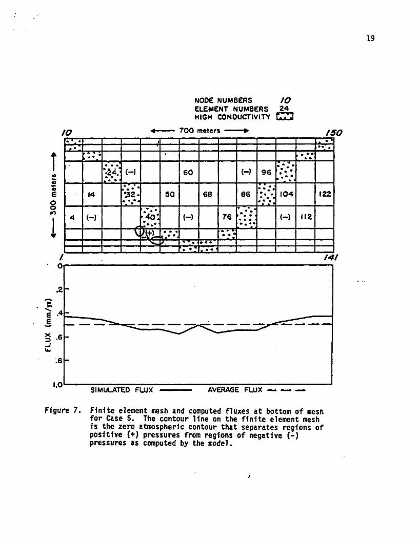
Case 5

Two relatively high hydraulic conductivity (K=1.26 mm/yr) inclined

columns of elements were used in this simulation. These relatively high

hydraulic conductivity elements were arranged diagonally in the otherwise

17

NODE NUMBERS /0ELEMENT NUMBERS 24LOW CONDUCTIVITY MI

/0 4- 700 meters - /50

E00

h.

-jxJ-

1.SIMULATED FLUX AVERAGE FLUX - -

Figure 6. Finite element mesh and computed fluxes at bottom of meshfor Case 4. The contour line on the finite element meshis the zero atmospheric contour that separates regions ofpositive (+) pressures from regions of negative (-)pressures as computed by the model.

18

average hydraulic conductivity matrix. The relatively permeable inclined

columns begin at each of the upper corners of the region modeled and dip

to the center of the base of the region modeled as shown in Figure 7.

This configuration is analogous to two relatively permeable fault zones

that dip and intersect. The simulation was run for 1,500 years prior to

reaching steady state.' The results are quantified in Figure 7. The flux

is greatest along the aforementioned diagonal, high conductivity

elements. The net result is greater flux--at the center of the discharge

face. The flux varies spatially from 0.43 mm/yr to 0.58 mm/yr throughout

the region modeled. Two nodes show positive pressures; however, these

are the result of round off errors in the program and are only slightly

positive. The pressures at the remainder of the nodes are negative.

Case 6

In this case, a high hydraulic conductivity value of 1.26 mrnyr

(Peters et al., 1984) was assigned to 22 elements throughout the flow

region as shown in Figure 8. These elements were selected using a random

number table. The remaining elements were assigned a hydraulic

conductivity value of 0.601 mm/yr. Geologically this case could reflect

differential depositional patterns or variable cooling rates near the

surfaces of strata that are distributed throughout the formation. Flow

was simulated for 1,500 years prior to achieving steady state conditions.

In this particular case, even though the locations of the rock

represented by the elements with high hydraulic conductivity were

generated randomly, the high hydraulic conductivity elements tend to

group at the left and right sides of the region. This grouping produces

the nonuniform distribution of downward flux shown in Figure 8. The

outflow varies spatially from 0.44 mm/yr to 0.61 mm/yr among nodes.

19


J024

/0 4- 700 meters -* /50

T00to

0

9~ . ..-

Z . o4*4 .

~~~~~* .'

I

.21

'a

E2..x-JU&.

41-.

- -- - - - - - --

.61-

.81-

1.O1SIMULATED FLUX - AVERAGE FLUX - --


20


/024

O0 4- 700 meters -- /50

jT

0

ES8

_ _ _ A~~. - -n -

..- (-) _ _t .. ;., _ orT.

_ _60__ 9 __ _

, 14 s2 68 86 104' 122

-- 40 76 - -:--112 -

_ _ _ > A: _ _ (I + + _~~~~~~w_'0~~4 .o

J r

31%

SIMULATED FLUX - AVERAGE FLUX - - -


21

Nodes with positive pressures also are shown in Figure 8. This

simulation demonstrates that even with a hydraulic conductivity field

selected randomly, the distribution of vertical flux may not be uniform

and that positive pressures can develop.

Case 7

Simulation number 7 employed the same arrangement of hydraulic

conductivity as the simulation for Case 6 but with a recharge rate of

0.6 mm/yr at the upper surface. The simulation was run for 1,500 years

prior to reaching steady state. The results are quantified in Figure 9.

The higher recharge rate produced fully saturated conditions in many of

the average hydraulic conductivity elements (K=0.601 mm/yr). The regions

which developed positive pressures are shown in Figure 9. Pressures as

great as 7.6 meters of water developed at some node points. The flux

varies spatially from 0.53 mm/yr to 0.69 ml/yr throughout the region

modeled. The distribution of flux is very similar to that of Case 6,

even though about one-third of the node points developed positive

pressures.

Case 8

In Case 8 the same random distribution of hydraulic conductivities

as discussed in Case 6 was used. However, low hydraulic conductivity

(K=0.211 mn/yr) values (rather than high conductivity values) were

assigned to the randomly selected elements. The input flux was set at

0.5 mm/yr, as in Case 6. The results are quantified in Figure 10. The

flux varies spatially from 0.4 mm/yr to 0.61 mm/yr throughout the region

modeled. The regions with positive pressures also are identified in

Figure 10. This simulation shows that the existence of low conductivity

22


/024

4 700 meters -4

00o

LI

SIMULATED FLUX AVERAGE FLUX - - -

Figure 9. Finite element mesh and computed fluxes at bottom of meshfor Case 7. The contour line on the finite element meshis the zero atmospheric contour that separates regions ofpositive (4) pressures from regions of negative (-)pressures as computed by the model.

23

NOOD NUMBERSELEMENT NUMBERSLOW CONDUCTIVITY

/024

4- 700 meters -5-b I0

¶T

Zco

0in

if I0

.2F

.63-%

I-1

PP :: lc--�I

.81-

1.0SIMULATED FLUX - AVERAGE FLUX - - -


V

24

(K=0.201 mm/yr) rock in 22 out of 126 elements produces positive

pressures in well over half of the region modeled at a recharge rate of

0.5 mm/yr.

Discussion of Results

Vertical fault zoqes or other geologic features of higher or lower

hydraulic conductivity rock of the size used in simulations 2 and 3 (50

meters) have not been mapped In Yucca Mountain. However, the range of

conductivity values used in the study is less than the range that has

been measured within Yucca Mountain by Peters et al. (1984).

Consequently our simulations may not reflect the maximum possible effects

of heterogeneities within the Topopah Spring Member.

The results of the first three simulations show that water moves

laterally because of pressure gradients induced by vertically oriented

high-permeability heterogeneities in the rock. The result is a

nonuniform horizontal distribution of downward flux. Flux is greater

through the elements of relatively high conductivity than through the

elements of average conductivity; areas of positive pressure do not

develop with the first three cases with a recharge rate of 0.5 mm/yr.

Pressures become greater than atmospheric pressure (positive) if the flux

is greater than the saturated conductivity of the low conductivity

elements (Case 4); as a portion of the rock becomes saturated, water

moves toward adjacent areas. In Case 4, the greater flux in the elements

of average conductivity also causes positive pressures to develop in the

average conductivity material (Figure 4).

25

Cases 5 through 8 are perhaps less hypothetical than the first four

cases because the latter reflect vertical variations in hydraulic

properties in addition to horizontal variations. The results of

simulations 5 through 8 illustrate that variability of hydraulic

conductivity in the vertical direction often will produce positive

pressures in the lower conductivity rock where it underlies higher

conductivity rock. Positive pressures occur because the high

conductivity rock at a higher elevation will carry more flux than the

lower conductivity rock. When this greater flux moves downward into the

lower conductivity rock it causes complete saturation and positive

pressures. These positive pressures then must dissipate horizontally as

the flux is redistributed in the horizontal plane. This situation is

shown in Figures 6, 8, 9 and 10.

Positive fluid pressures are important because all pores (including

fractures or open fault zones) will accept flow under such conditions.

Consequently, much shorter travel times through the profile may occur

compared to the case where only matrix flow occurs. Our study shows that

it will be necessary to consider the heterogeneities of rock properties

in order to predict the distribution of downward flux. It also will be

necessary to delineate the scale of heterogeneities in order to select a

mesh size for simulation. If this procedure is not followed, simulations

may not account for regions of positive pressure and fracture flow.

The following factors should be emphasized with respect to the

results of this series of simulations.

1) Only matrix flow of liquid water is simulated; flow through

discrete fractures, vapor flow, and heat flow are not included

specifically. If the vertical columns of elements discussed herein

26

are envisioned to be fault zones they must be filled with gouge or

other porous rock. Discrete fracture flow is not treated in the

models discussed in this paper. Faults that display open fractures

will not function hydraulically like the heterogeneities described

herein (see Wang and Narasimhan, 1984).

2) Only flow in the jopopah Spring Member of the Paintbrush Tuff

Formation is considered, as analyzed by Montazer and Wilson (1984),

Wilson (1985) and Peters et al. (1984). The bedding of the rocks is

assumed to be horizontal. The true dip (see Figure 2) of the

Topopah Spring Member was not simulated.

3) Three of the eight conditions simulated are analogous to fault or

fracture zones that contain either relatively higher or lower

permeability. Hydraulic conditions simulated around these zones are

realistic if any fracture flow that may be present can be treated as

an equivalent porous medium.

4) We have assumed uniform spatial distribution of recharge in

accordance with Montazer and Wilson (1984). In reality the recharge

rate will vary with permeability. However the recharge flux should

redistribute according to permeability soon after it enters the

Topopah Spring Member. Investigation of the true effect of

nonuniform recharge is left to future work.

5) We have simulated the bottom of the Topopah Spring Member as the

water table. The only alternative is to Input measured pressures at

the bottom of the Topopah Spring Member. The insertion of real

pressures is left to future work after the appropriate pressures

have been measured.

27

Conclusions

These computer simulations using UNSAT2 justify the following

conclusions.

1) Heterogeneities in a porous rock matrix will cause downward flux in

the unsaturated zone to be distributed nonuniformly in the

horizontal plane.

2) Positive pressures tend to develop in some zones in which the

saturated hydraulic conductivity of the matrix is less than the

downward flux (see for example Figure 6). This condition, where it

occurs, will produce preferential flow paths. Flow into fractures

may occur at such locations if discrete, open fractures intercept

these zones of positive pressures; however, we did not simulate such

flow. Continuous fracture flow through the entire unit, if it

occurs, could reduce the ground water travel time to the accessible

environment considerably. Flow through fractures could also reduce

some pressures to atmospheric.

3) The effect of heterogeneities on flow in the unsaturated zone cannot

be predicted intuitively. Quantification by a modeling process such

as the one used herein is required.

4) A one-dimensional analysis of flow in the Topopah Spring Member of

the Paintbrush Tuff Formation within Yucca Mountain is insufficient

to ensure that nonuniform downward flux or fracture flow do not

occur.

5) If the spatial average downward flux is 0.5 mm/yr as expressed by

Montazer and Wilson (1984) (or greater) and if the permeability

values presented by Peters et al. (1984) are representative, then

regions of positive pressure probably exist in the tuffs of Yucca

28

Mountain. If the values are valid, positive pressures will develop

wherever the saturated hydraulic conductivity is less than 0.5

nm/yr. This result illustrates the necessity for measuring recharge

rates and hydrogeologic properties at the appropriate scale.

6) The results of the simulations presented herein illustrate the

necessity for delineating in detail the spatial distribution of

hydraulic conductivity in the unsaturated zone within Yucca

Mountain. The results quantified herein illustrate that modeling of

the downward flux should be conducted in at least two dimensions.

Delineation of populations of hydraulic conductivity values

according to spatial distribution may be feasible using the

statistical procedure discussed by Steinhorst and Williams (1985).

7) Documentation of the absence of regions of positive pressure would

constitute the best evidence in support of the concept of exclusive

matrix flow rather than a combination of matrix flow and fracture

flow in the Topopah Spring Member of the Paintbrush Tuff Formation.

Acknowledgements

This study was commissioned by the Hydrology Section of the High-

Level Waste Management Division of the U.S. Nuclear Regulatory Commission

in Washington, D.C. under Contract No. NRC-02-85-008. The individuals

who are specifically responsible for initiating the study are Mr. Jeff

Pohle and Mr. William Ford. However, the NRC does not necessarily agree

with the findings of the study.

29

References

Bloomsburg, G.L., and Wells, R.D., 1978, Seepage Through PartiallySaturated Shale Wastes. Final report on Contract No. H0252065, U.S.Dept. of Interior, Bureau of Mines.

Davis, L.A., and Neuman, S.P., December 1983, Documentation and User'sGuide UNSAT2 - Variably Saturated Flow Model. Prepared for Divisionof Waste Management, U.S. Nuclear Regulatory Commission, NUREG/CR-3390.

Mualem, Y., 1976, A New Model for Predicting .the Hydraulic Conductivityof Unsaturated Porous Materials. Water Resources Research, vol. 12,no. 3, p. 513-522.

Montazer, P., and Wilson, W.E., 1984, Conceptual Hydrologic Model of Flowin the Unsaturated Zone, Yucca Mountain, Nevada. U.S. GeologicalSurvey, Lakewood, CO, Water Resources Investigations Report, USGS-WRI-84-4345.

Neuman, S.P., Feddes, R.A., and Bresler, E., 1974, Finite ElementSimulation of Flow in Saturated-Unsaturated Soils Considering WaterUptake by Plants. Israel Institute of Technology, Haifi, Israel,104 p.

Peters, R.R., et al., 1984, Fracture and Matrix HydrologicCharacteristics of Tuffaceous Materials from Yucca Mountain, NyeCounty, Nevada. Sandia National Laboratories, Albuquerque, NM,SAND84-1471.

Peters, R.R., and Klavetter, E.A., 1988, A Continuum Model for WaterMovement in an Unsaturated Fractured Rock Mass. Water ResourcesResearch, vol. 24, no. 3, p. 416-430.

Sinnock, S., Lin, Y.T., and Brannen, J.P., 1984, Preliminary Bounds onthe Expected Postclosure Performance of the Yucca MountainRepository Site, Southern Nevada. Sandia National Laboratories,Albuquerque, NM, SAND84-1492.

Sinnock, S., Lin, Y.T., Tierney, M.S., et al., 1986, PreliminaryEstimates of Groundwater Travel Time and Radionuclide Transport atthe Yucca Mountain Repository Site. Sandia National Laboratories,Albuquerque, NM and Livermore, CA, SAND85-2701.

Steinhorst, R.K., and Williams, R.E., 1985, Discrimination of GroundwaterSources Using Cluster Analysis, MANOVA, Canonical Analysis andDiscriminant Analysis. Water Resources Research, vol. 21, no. 8, p.1149-1156.

U.S. Department of Energy, 1986, Environmental Assessment, Yucca MountainSite, Nevada Research and Development Area, Nevada. DOE/RW-0073,Washington, D.C.

30

van Genuchten, R., 1978, Calculating the Unsaturated HydraulicConductivity with a New Closed Form Analytical Model. WaterResources Bulletin, Princeton University Press, PrincetonUniversity, Princeton, NJ.

Wang, J.S.Y., and Narasimhan, T.N., 1985, Hydrologic Mechanisms GoverningFluid Flow in Partially Saturated, Fractured, Porous Tuff at YuccaMountain. Sandia National Laboratories, Albuquerque, NM, SAND84-7202, 47 p.

Wilson, W.W., 1985, Letter from W.W. Wilson (USGS) to D.L. Vieth(DOE/NVO), December 24, 1985; regarding unsaturated zone flux.

Distribution of Downward Flux in Unsaturated …downward flow should be anticipated in heterogeneous...

Documents

Transcript of Distribution of Downward Flux in Unsaturated …downward flow should be anticipated in heterogeneous...